Detection and location of 127 anatomical landmarks indiverse CT datasets

Mohammad A. Dabbah, Sean Murphy, Hippolyte Pello, Romain Courbon, Erin Beveridge,Stewart Wiseman, Daniel Wyeth, Ian Poole

Toshiba Medical Visualization Systems Europe Ltd., Bonnington Bond, 2 Anderson Place,Edinburgh EH6 5NP, UK

ABSTRACT

The automatic detection and localization of anatomical landmarks has wide application, including intra and inter-patient registration, study location and navigation, and the targeting of specialized algorithms. In this paper,we demonstrate the automatic detection and localization of 127 anatomically defined landmarks distributedthroughout the body, excluding arms. Landmarks are defined on the skeleton, vasculature and major organs.Our approach builds on the classification forests method,1 using this classifier with simple image features whichcan be efficiently computed. For the training and validation of the method we have used 369 CT volumes on whichradiographers and anatomists have marked ground truth (GT) — that is the locations of all defined landmarksoccurring in that volume. A particular challenge is to deal with the wide diversity of datasets encountered inradiology practice. These include data from all major scanner manufacturers, different extents covering singleand multiple body compartments, truncated cardiac acquisitions, with and without contrast. Cases with stentsand catheters are also represented. Validation is by a leave-one-out method, which we show can be efficientlyimplemented in the context of decision forest methods. Mean location accuracy of detected landmarks is 13.45mmoverall; execution time averages 7s per volume on a modern server machine. We also present localization ROCanalysis to characterize detection accuracy — that is to decide if a landmark is or is not present in a givendataset.

Keywords: anatomical landmarks, decision forests, ROC analysis, computed tomography

1. INTRODUCTION

The technical goal of this work can be stated as: given a previously unseen volumetric CT dataset, from alarge set of pre-defined anatomical meaningful landmarks identify which are present (“detection”), and find theirmost likely position (“location”). Although DICOM datasets often include tags indicating anatomical region, wehave found these to be inconsistent and unreliable across vendors and institutions; thus we make no use of suchtags. Landmark detection underpins a semantic understanding of the medical data and thus has many diverseapplications, for example, it facilitates rapid navigation to a named organ. There is a close duality betweenlandmark location and image registration. Given corresponding landmarks in a pair of datasets, registration isstraightforward. Conversely, inter-patient registration allows landmarks manually marked on one dataset (an“atlas”) to be transferred to the second, thus achieving automatic landmark detection.

In the last decade, research in anatomical landmark detection and localization has been active and growingrapidly. Worz & Rohr2,3 initially proposed a method to detect and localize landmarks in 3D CT and MR imagesusing parametric intensity models of anatomical structures via Gaussian error function in conjunction with 3Drigid transformations and deformable ellipsoidal shape fitting. Another geometric method4 based on convolutionand 4D graph-cuts was proposed to segment organs from 4D contrast-enhanced abdominal CT data.

Anatomical landmarks and structure detection features strongly in multi-organ extraction and segmentation.Shimizu et al.5,6 was among the first to describe an atlas-based method for simultaneous multi-organs segmen-tation/extraction. This method was based on an EM algorithm and multiple level sets to finely segment organregions. Many other articles were published presenting atlas-based solutions to the problem — see 7–9 just toname a few.

Other approaches use machine learning algorithms. Criminisi et al.1 have described a classification randomdecision forest to identify the bounding boxes of organs. This work has been further extended to a regressionforest,10 generative-discriminative model,11 the so-called entangled decision forests,12 and random ferns.13

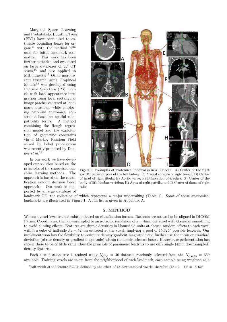
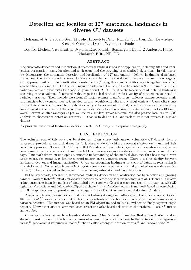
Figure 1. Examples of anatomical landmarks in a CT scan. A) Center of the righteye; B) Superior pole of the left kidney; C) Medial condyle of right femur; D) Centerof head of right fibula; E) Aortic valve; F) Bifurcation of trachea; G) Center of thebody of 5th lumbar vertebra; H) Apex of right patella; and I) Center of dome of righttalus

Marginal Space Learningand Probabilistic Boosting Trees(PBT) have been used to es-timate bounding boxes for or-gans14 with the method of15

used for initial landmark esti-mation. This work has beenfurther extended and evaluatedon large databases of 3D CTscans,16 and also applied toMR datasets.17 Other more re-cent research using GraphicalModels18 was developed usingPictorial Structure (PS) mod-els with local appearance inte-gration using local rectangularimage patches centered at land-mark locations, while employ-ing pair-wise anatomical con-straints based on spatial com-patibility terms. A methodcombining the Hough regres-sion model and the exploita-tion of geometric constrainsvia a Markov Random Fieldsolved by belief propagationwas recently proposed by Don-ner et al.19

In our work we have devel-oped our solution based on theprinciples of the supervised ma-chine learning methods. Theapproach is based on the classi-fication random decision forestapproach.1 Our work is sup-ported by a large database oflandmark GT, the collection of which represents a major undertaking (Table 1). Some of these anatomicallandmarks are illustrated in Figure 1. A full list is given in Appendix A.

2. METHOD

We use a voxel-level trained solution based on classification forests. Datasets are rotated to be aligned in DICOMPatient Coordinates, then downsampled to an isotropic resolution of s = 4mm per voxel with Gaussian smoothingto avoid aliasing effects. Features are simple densities in Hounsfield units at chosen random offsets to each voxelwithin a cube of half-side Fd = 52mm centered at the voxel, implying a pool of 15,625∗ possible features. Ourimplementation has the flexibility to compute density gradient magnitude and further use the mean or standarddeviation (of raw density or gradient magnitude) within randomly selected boxes. However, experimentation hasshown these to be of little value, thus the principle of parsimony leads us to use only single (4mm downsampled)density features.

Each classification tree is trained using Ndpt = 40 datasets randomly selected from the Ndsets = 369

available. Training voxels are taken from the neighborhood of each landmark, each sample being weighted as a

∗half-width of the feature ROI is defined by the offset of 13 downsampled voxels, therefore (13 ∗ 2 − 1)3 = 15, 625

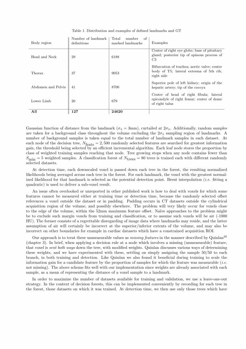
Table 1. Distribution and examples of defined landmarks and GT

Body regionNumber of landmarkdefinitions

Total number ofmarked landmarks Examples

Head and Neck 29 6188

Center of right eye globe; base of pituitarygland; posterior tip of spinous process ofC3

Thorax 37 9053

Bifurcation of trachea; aortic valve; centerbody of T5; lateral extrema of 5th rib,right side

Abdomen and Pelvis 41 8700Superior pole of left kidney; origin of thehepatic artery; tip of the coccyx

Lower Limb 20 679

Center of head of right fibula; lateralepicondyle of right femur; center of domeof right talus

All 127 24620

Gaussian function of distance from the landmark (σλ = 3mm), curtailed at 2σλ. Additionally, random samplesare taken for a background class throughout the volume excluding the 2σλ sampling region of landmarks. Anumber of background samples is taken equal to the total number of landmark samples in each dataset. Ateach node of the decision tree, Nfeats = 2, 500 randomly selected features are searched for greatest informationgain, the threshold being selected by an efficient incremental algorithm. Each leaf node stores the proportion byclass of weighted training samples reaching that node. Tree growing stops when any node contains fewer thanSmin = 5 weighted samples. A classification forest of Ntrees = 80 trees is trained each with different randomlyselected datasets.

At detection time, each downscaled voxel is passed down each tree in the forest, the resulting normalizedlikelihoods being averaged across each tree in the forest. For each landmark, the voxel with the greatest normal-ized likelihood for that landmark is selected as the potential detection point. Brent interpolation (i.e. fitting aquadratic) is used to deliver a sub-voxel result.

An issue often overlooked or unreported in other published work is how to deal with voxels for which somefeatures cannot be measured either at training time or detection time, because the randomly selected offsetreferences a voxel outside the dataset or in padding. Padding occurs in CT datasets outside the cylindricalacquisition region of the volume, and possibly elsewhere. The problem will very likely occur for voxels closeto the edge of the volume, within the 52mm maximum feature offset. Naıve approaches to the problem mightbe to exclude such margin voxels from training and classification, or to assume such voxels will be air (-1000HU). The former consists of a regrettable disregarding of image data where landmarks may reside, and the latterassumption of air will certainly be incorrect at the superior/inferior extents of the volume, and may also beincorrect on other boundaries for example in cardiac datasets which have a constrained acquisition ROI.

Our approach is to treat these unmeasurable values as missing features in the manner described by Quinlan20

(chapter 3). In brief, when applying a decision rule at a node which involves a missing (unmeasurable) feature,that voxel is sent both ways down the tree, with modified weights. Quinlan discusses various ways of determiningthese weights, and we have experimented with these, settling on simply assigning the sample 50/50 to eachbranch, in both training and detection. Like Quinlan we also found it beneficial during training to scale theinformation gain for a candidate feature by the proportion of samples for which the feature was measurable (i.e.not missing). The above scheme fits well with our implementation since weights are already associated with eachsample, as a mean of representing the distance of a voxel sample to a landmark.

In order to maximize the number of datasets available for training and validation, we use a leave-one-outstrategy. In the context of decision forests, this can be implemented conveniently by recording for each tree inthe forest, those datasets on which it was trained. At detection time, we then use only those trees which have

not seen the dataset in question. Thus, the effective size of the classification forest on a particular validation

dataset is somewhat smaller than the Ntrees trees which were trained, typically Ntrees(1 −NdptNdsets

) ≈ 71 trees

in our experiments. We call this reduced collection of trees a denuded forest. This scheme allows for efficientexperimentation, avoiding repeated training for each dataset. We nevertheless acknowledge that the variousmeta parameters - Fd, s, Ndpt, σλ, Nfeats — have been optimized with sight of all datasets, leading to the

possibility of over-fitting and optimistic estimation of accuracy. Given the large number and diversity of datasetswe believe such over-fitting to be small.

2.1 Application of a point atlas to automatic landmarking

Figure 2. The point atlas. The sphere radii represent therelative standard deviations of the point positions (not usedin method — visualization only).

The classification approach above generates candidatelandmarks substantially independently of one another;it takes no advantage of the predictable spatial rela-tionships between landmarks. A simple point atlas isused here to exploit these spatial relationships.

The point atlas is created off-line by registering allground truth collections to a typical full body datasetby minimization of sum-square distance over the set ofaffine transformations, and aggregating these togetherto single mean point estimates. When presented witha novel dataset, the decision forest detection generatescandidate points with a certainty equal to the normal-ized likelihood for the assigned class. These candi-date points are subsequently matched with the pointatlas using an affine transform. The contribution ofeach point in determining the transform is weightedby its certainty, and a trimmed least squares approachis employed to make the fitting robust. Subsequently,logistic regression is used to recalculate the certaintyof each point as a posterior probability, given the dis-tance of its current location from that predicted bythe point atlas, and the original certainty, given bythe decision forest. This process considerably reducesthe occurrence of false positive landmarks, with onlya small detrimental effect on the true positives. Thusthe mean distance between true positive landmarksand their ground truth locations is reduced (see re-sults in Section 3.4).

Finally, since any dataset typically contains only asubset of landmarks, thus potential points are filtered by the point atlas certainty threshold τPoint Atlas .

3. GROUND TRUTH AND EXPERIMENTAL RESULTS

3.1 Landmark definition and ground truth collection

Landmarks were defined based on anatomical coverage, the clarity of location and their clinical utility. The 127anatomical points span a range of different tissues and organs throughout the body, however we have not yetincluded arms. See Appendix A for a full list and brief description of each of these landmarks. To optimizeaccuracy and assume a consistent interpretation of landmarks, a carefully-defined protocol was followed. Eachlandmark has an accompanying description, example image and the marking plane — axial, coronal or sagittal— is defined.

The 449 multi-vendor CT datasets on which ground truth was collected covers a wide range of anatomies,including contrast and non-contrast acquisitions, from multiple scanner vendors.

Ground truth was performed using an in-house tool which presents 3 orthogonal planes. An anatomicallytrained user manually locates each landmark in a dataset, the tool records and saves the position. Locationsare recorded in DICOM patient space. For cases where ambiguity of the position may exist, for example wherethe landmark is obscured by pathology yet its presence is assured, the landmark is recorded as “uncertain”.Such landmarks are excluded from training and from determination of location error, but are included in ROCdetection analysis.

We have tried to make the mix of datasets representative, and to this end we have taken out half of our headcases since these were over represented. A few highly anomalous datasets have also been excluded, but we havemostly used all datasets to which we have access without prejudice. This explains why our results in Section 3.4refer to 369 (not 449) datasets.

3.2 Algorithm Parameters Tuning

Our overall solution has a number of parameters which influence the trade-off between accuracy (location errorand detection AUC (Section 3.4)) and runtime. The key parameters are:

Training Forest Size (Ntrees) This is the number of trees to be trained in one decision forest and is set to80 by default. Runtime increases roughly linearly with forest size. In one experiment we observed anapproximately 2mm decrease in mean distance error when increasing forest size from 80 to 250. However,the runtime increases around four fold.

Number of Datasets per Tree (Ndpt) Using more dataset to train a tree results in more samples for each

landmark and more background coverage. The tree thus grows to a greater depth, increasing classificationaccuracy at the cost of runtime. Memory usage during training can also become an issue. A furtherconsequence of increasing Ndpt is that the size of the denuded forest in leave-one-out validation is reduced.

Skip factor During detection, rather than evaluating the likelihood at every downsampled voxel in the noveldataset, voxels are sampled at intervals determined by a “skip factor”. We settled on a skip factor of 2,thus speeding detection by a factor of ∼ 8. Location accuracy is not significantly effected, due to the useof Brent interpolation when locating the maximum, as described above.

3.3 Evaluation Criteria

The evaluation is based on two key independent measures:

Location error: The location error for landmark detection is the Euclidean distance, in mm, between theground truth landmark position and the detected landmark position. We report the mean and median locationerror over all landmarks in the ground truth — i.e. true positives and false negatives, thus these statistics areindependent of the detection operating point.

Detection AUC: Also known as the “area under the receiver operating characteristic (ROC) curve”. This is ameasure of the system’s ability to decide whether a landmark is present or not. The ROC curve is parametrizedby a certainty threshold, which determines the “operating point” i.e. the trade-off between false positive andfalse negative rates. We report detection AUC for a range of location error distances, with infinite distance beinginterpreted as “landmark present somewhere in the dataset”.

Together, these two measures provide convenient independent characterization of the system’s accuracy, forlocation and detection respectively. A further useful criteria which we will sometimes refer to is the true positive(TP) mean distance location error. This is the mean distance location error taken over only those landmarksclassified as “detected”, and is thus dependent on the chosen ROC operating point — i.e. . the certaintythreshold.

Of course, these statistics are influenced by the mix of datasets used, since some regions are more problematicthan others; as seen in Table 2 we do well in the head, but the thorax is difficult due to repeated structures.

HNB1.A

HNB12.IHNB13.I

HNB14.AHNB15.A

HNB2.S

HNB3.SHNB4.S

HNB5.C HNB6.C

HNB7.C HNB8.C

HNB9.C

X HNB16.C

HNB22.P

(a)

HNB1.A

HNB12.IHNB13.I

HNB14.AHNB15.A

HNB2.S

HNB3.SHNB4.S

HNB5.CHNB6.C

HNB7.CHNB8.C

HNB9.C

X HNB16.C

HNB22.P

(b)

HNB1.A

HNB10.SHNB11.S

HNB12.I HNB13.I

HNB17.C

HNB18.C

HNB19.C

HNB2.S

HNB20.C

HNB21.C

HNB22.P

HNB23A.P

HNB3.S

HNB5.C HNB6.CHNB7.C

HNB8.C

HNB9.C

THOR15.S

THOR2.S THOR26.C

THOR27.C

THOR3.S

THOR6.C

THOR7.CTHOR8.C

THOR9.C

X THOR1.C

X THOR28.C

X THOR32.R

HNB16.C

HNB23B.P

HNB24.P

HNB25.P

HNB26.P

HNB27.P

HNB28.P

HNB4.S

THOR20.A

THOR21.A

(c)

HNB1.A

HNB10.SHNB11.S

HNB12.IHNB13.I

HNB17.C

HNB18.C

HNB19.C

HNB2.S

HNB20.C

HNB21.C

HNB22.P

HNB23A.P

HNB3.S

HNB5.CHNB6.CHNB7.CHNB8.C

HNB9.C

THOR15.S

THOR2.STHOR26.C

THOR27.C

THOR3.S

THOR6.C

THOR7.CTHOR8.C

THOR9.C

X THOR1.C

X THOR28.C

X THOR32.R

HNB16.C

HNB23B.P

HNB24.P

HNB25.P

HNB26.P

HNB27.P

HNB28.P

HNB4.S

THOR20.A

THOR21.A

(d)

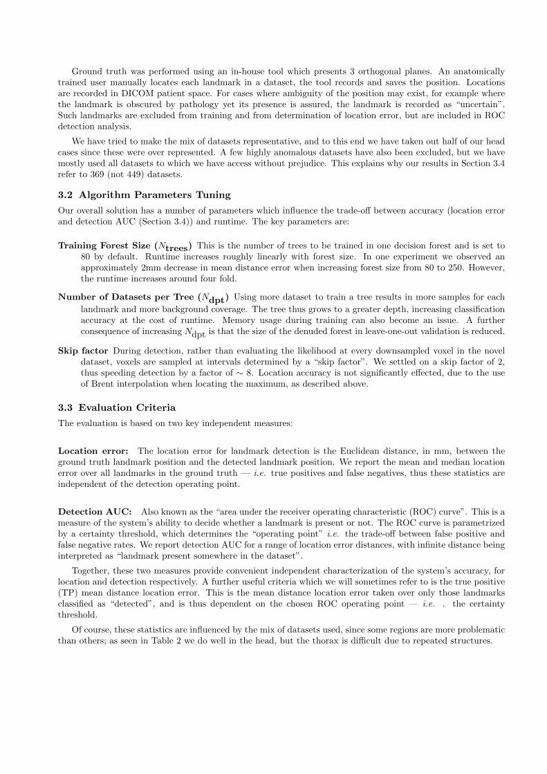
Figure 3. Automatically detected Head, Head/Neck & Upper Thorax landmarks positioned on: (a and c) are coronalMIPs and (b and d) are sagittal MIPs of novel CT scans. (Note that the Pineal Gland (HNB16.C) is missing from theground truth in (a). Refer to Appendix A for landmarks descriptions.

3.4 Whole Body CT Results

The evaluation of detection and localization of 127 anatomical landmarks in CT datasets is performed on all369 CT datasets from 6 different body compartments covering the entire human body except the arms. Theaverage processing time to automatically-identify and localize all landmarks in a given CT scan is approximately7 seconds on a 24 core computer.

Leave-one-out training and validation is performed using a denuded forest as described above.

Visual illustrations of the automatically-detected landmarks positioned on the novel CT scans from variousbody regions are shown in Figure 3 to Figure 5. A brief description of the landmarks shown is listed in Ap-pendix A.

THOR1.C

THOR13.L

THOR15.S

THOR16.R

THOR17.L

THOR18.S

THOR19.S

THOR2.S

THOR20.A

THOR21.A

THOR22.ATHOR23.A

THOR24.A THOR25.A

THOR26.C

THOR27.C

THOR28.C

THOR29.C

THOR3.S

THOR30.C

THOR31.C

THOR32.RTHOR33.L

THOR34.RTHOR35.L

THOR36.R THOR37.L

THOR4.I THOR5.I

THOR6.CTHOR7.C

THOR8.C

THOR9.C

X ABDO8.P

X HNB21.CX HNB28.P

X THOR10.C

X THOR11.C

(a)

THOR1.C

THOR13.L

THOR15.S

THOR16.R

THOR17.L

THOR18.S

THOR19.S

THOR2.S

THOR20.A

THOR21.A

THOR22.ATHOR23.A

THOR24.ATHOR25.A

THOR26.C

THOR27.C

THOR28.C

THOR29.C

THOR3.S

THOR30.C

THOR31.C

THOR32.RTHOR33.L

THOR34.RTHOR35.L

THOR36.RTHOR37.L

THOR4.ITHOR5.I

THOR6.CTHOR7.CTHOR8.C

THOR9.C

X ABDO8.P

X HNB21.CX HNB28.P

X THOR10.C

X THOR11.C

(b)

ABDO1.SABDO11.C

ABDO12.CABDO13.C

ABDO14.C

ABDO15.C

ABDO16.C

ABDO17.C

ABDO18.C ABDO19.C

ABDO2.S

ABDO20.C

ABDO21.C

ABDO22.C

ABDO23.C

ABDO24.C

ABDO25.C

ABDO26.SABDO27.S

ABDO28.A

ABDO29.A

ABDO3.I

ABDO30.C

ABDO31.C ABDO32.CABDO33.S

ABDO34.L

ABDO35.S

ABDO36.L

ABDO37.S

ABDO38.I

ABDO39.S

ABDO4.I

ABDO40.I

ABDO41.I

ABDO6.L

ABDO7.I

ABDO8.PABDO9.C

THOR31.C

X THOR16.R

X THOR17.LX THOR24.A

X THOR25.A

X THOR37.L

ABDO10.C

ABDO5.M

(c)

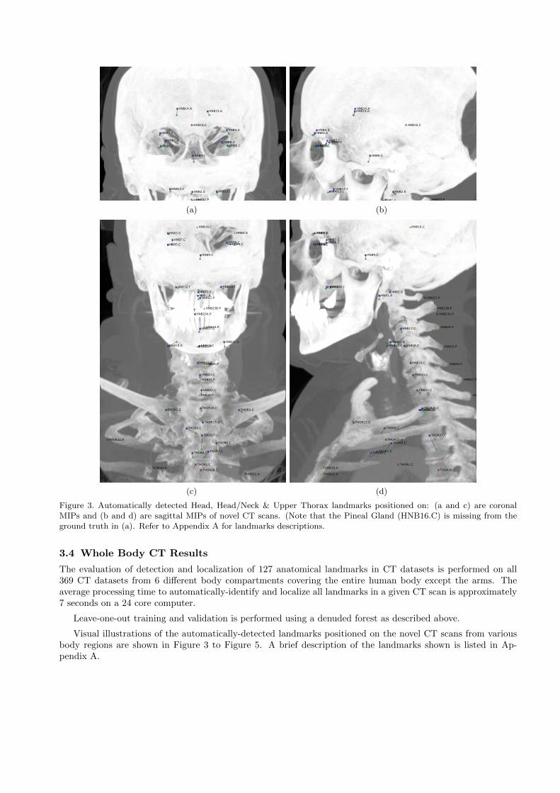
Figure 4. Automatically detected Thorax and Abdomen & Pelvis landmarks positioned on: (a and c) coronal MIPs and(b) a sagittal MIP of a novel CT scan. Refer to Appendix A for landmarks descriptions.

Detection results are shown against coronal and sagittal maximum intensity projection (MIP) images where:green dots indicate ground truth position; blue squares indicate the location of the correctly detected landmarks

LOWL1

LOWL10

LOWL11 LOWL12

LOWL13

LOWL14

LOWL15

LOWL16

LOWL17LOWL18

LOWL19

LOWL2

LOWL20

LOWL3LOWL4

LOWL5LOWL6

LOWL7LOWL8

LOWL9

(a)

LOWL1

LOWL10

LOWL11LOWL12

LOWL13

LOWL14

LOWL15

LOWL16

LOWL17LOWL18

LOWL19

LOWL2

LOWL20

LOWL3LOWL4

LOWL5LOWL6LOWL7LOWL8

LOWL9

(b)

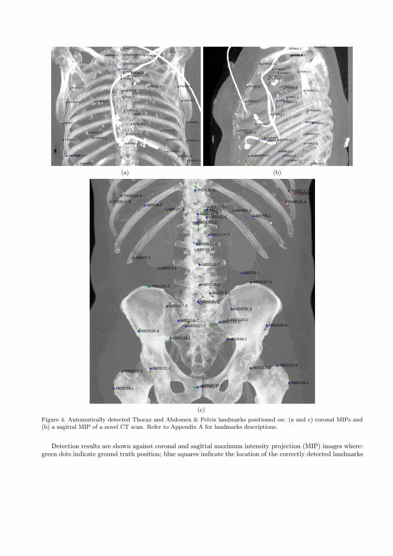
Figure 5. automatically detected Lower Limbs landmarks positioned on: (a) a coronal MIP and (b) a sagittal MIP of anovel CT scan. Refer to Appendix A for landmarks descriptions.

(true positives); yellow triangles indicate missed landmarks (false negatives); red crosses indicate falsely detectedlandmarks (false positives). Ground truth and detected positions for a landmark are linked by a line.

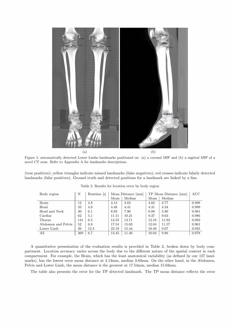
Table 2. Results for location error by body region

Body region N Runtime [s] Mean Distance [mm] TP Mean Distance [mm] AUCMean Median Mean Median

Brain 12 4.8 4.13 3.83 4.02 3.77 0.998Head 33 4.8 4.48 4.41 4.31 4.34 0.999Head and Neck 30 6.1 8.93 7.96 6.09 5.80 0.981Cardiac 62 5.1 11.11 10.21 9.37 9.63 0.986Thorax 141 6.5 14.55 13.71 12.18 11.93 0.983Abdomen and Pelvis 52 6.8 17.54 15.03 12.04 11.57 0.961Lower Limb 39 12.3 22.19 15.44 10.48 9.67 0.945

All 369 6.7 13.45 11.40 10.04 9.86 0.978

A quantitative presentation of the evaluation results is provided in Table 2, broken down by body com-partment. Location accuracy varies across the body due to the different nature of the spatial context in eachcompartment. For example, the Brain, which has the least anatomical variability (as defined by our 127 land-marks), has the lowest error mean distance at 4.13mm, median 3.83mm. On the other hand, in the Abdomen,Pelvis and Lower Limb, the mean distance is the greatest at 17.54mm, median 15.03mm.

The table also presents the error for the TP detected landmark. The TP mean distance reflects the error

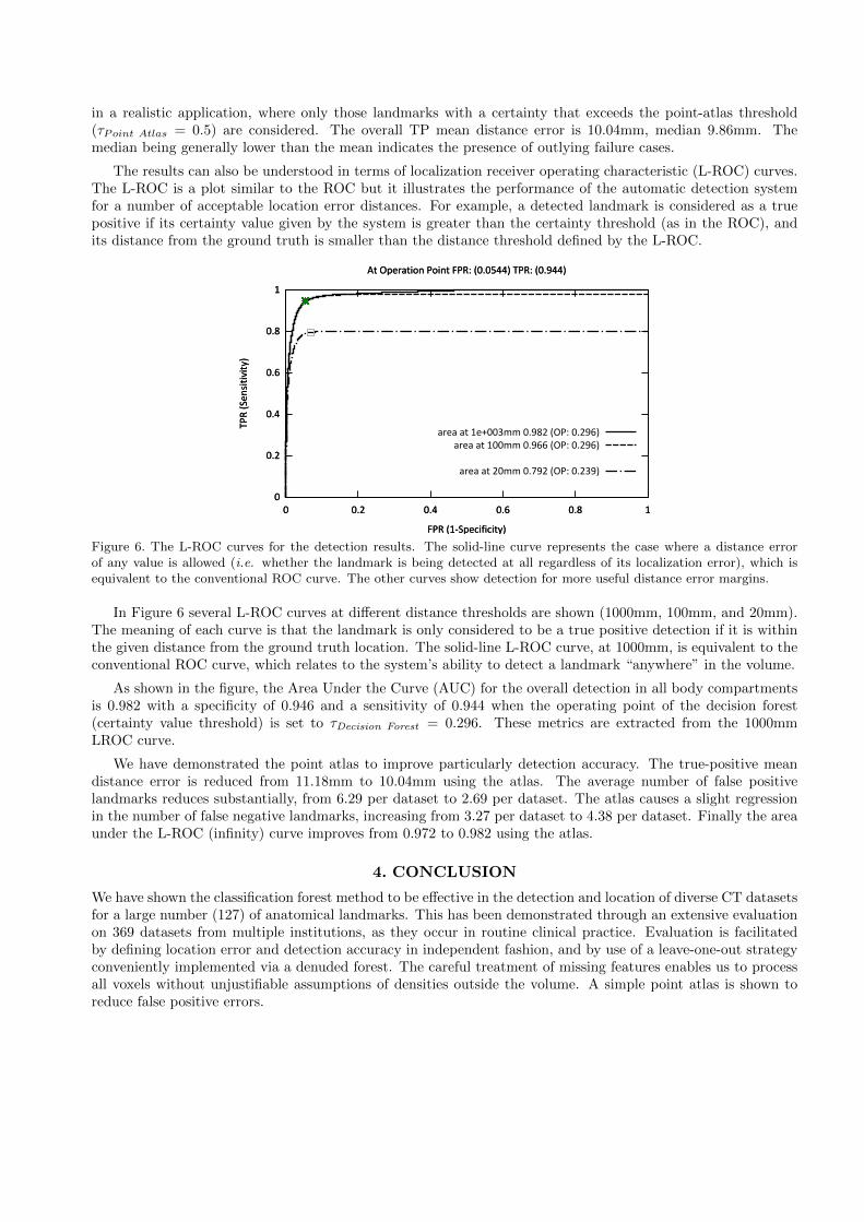
in a realistic application, where only those landmarks with a certainty that exceeds the point-atlas threshold(τPoint Atlas = 0.5) are considered. The overall TP mean distance error is 10.04mm, median 9.86mm. Themedian being generally lower than the mean indicates the presence of outlying failure cases.

The results can also be understood in terms of localization receiver operating characteristic (L-ROC) curves.The L-ROC is a plot similar to the ROC but it illustrates the performance of the automatic detection systemfor a number of acceptable location error distances. For example, a detected landmark is considered as a truepositive if its certainty value given by the system is greater than the certainty threshold (as in the ROC), andits distance from the ground truth is smaller than the distance threshold defined by the L-ROC.

0

0.2

0.4

0.6

0.8

1

0 0.2 0.4 0.6 0.8 1

TP

R (

Se

nsi

tiv

ity

)

FPR (1-Specificity)

At Operation Point FPR: (0.0544) TPR: (0.944)

area at 1e+003mm 0.982 (OP: 0.296)

area at 100mm 0.966 (OP: 0.296)

area at 20mm 0.792 (OP: 0.239)

0

0.2

0.4

0.6

0.8

1

0 0.2 0.4 0.6 0.8 1

TP

R (

Se

nsi

tiv

ity

)

FPR (1-Specificity)

At Operation Point FPR: (0.0544) TPR: (0.944)

Figure 6. The L-ROC curves for the detection results. The solid-line curve represents the case where a distance errorof any value is allowed (i.e. whether the landmark is being detected at all regardless of its localization error), which isequivalent to the conventional ROC curve. The other curves show detection for more useful distance error margins.

In Figure 6 several L-ROC curves at different distance thresholds are shown (1000mm, 100mm, and 20mm).The meaning of each curve is that the landmark is only considered to be a true positive detection if it is withinthe given distance from the ground truth location. The solid-line L-ROC curve, at 1000mm, is equivalent to theconventional ROC curve, which relates to the system’s ability to detect a landmark “anywhere” in the volume.

As shown in the figure, the Area Under the Curve (AUC) for the overall detection in all body compartmentsis 0.982 with a specificity of 0.946 and a sensitivity of 0.944 when the operating point of the decision forest(certainty value threshold) is set to τDecision Forest = 0.296. These metrics are extracted from the 1000mmLROC curve.

We have demonstrated the point atlas to improve particularly detection accuracy. The true-positive meandistance error is reduced from 11.18mm to 10.04mm using the atlas. The average number of false positivelandmarks reduces substantially, from 6.29 per dataset to 2.69 per dataset. The atlas causes a slight regressionin the number of false negative landmarks, increasing from 3.27 per dataset to 4.38 per dataset. Finally the areaunder the L-ROC (infinity) curve improves from 0.972 to 0.982 using the atlas.

4. CONCLUSION

We have shown the classification forest method to be effective in the detection and location of diverse CT datasetsfor a large number (127) of anatomical landmarks. This has been demonstrated through an extensive evaluationon 369 datasets from multiple institutions, as they occur in routine clinical practice. Evaluation is facilitatedby defining location error and detection accuracy in independent fashion, and by use of a leave-one-out strategyconveniently implemented via a denuded forest. The careful treatment of missing features enables us to processall voxels without unjustifiable assumptions of densities outside the volume. A simple point atlas is shown toreduce false positive errors.

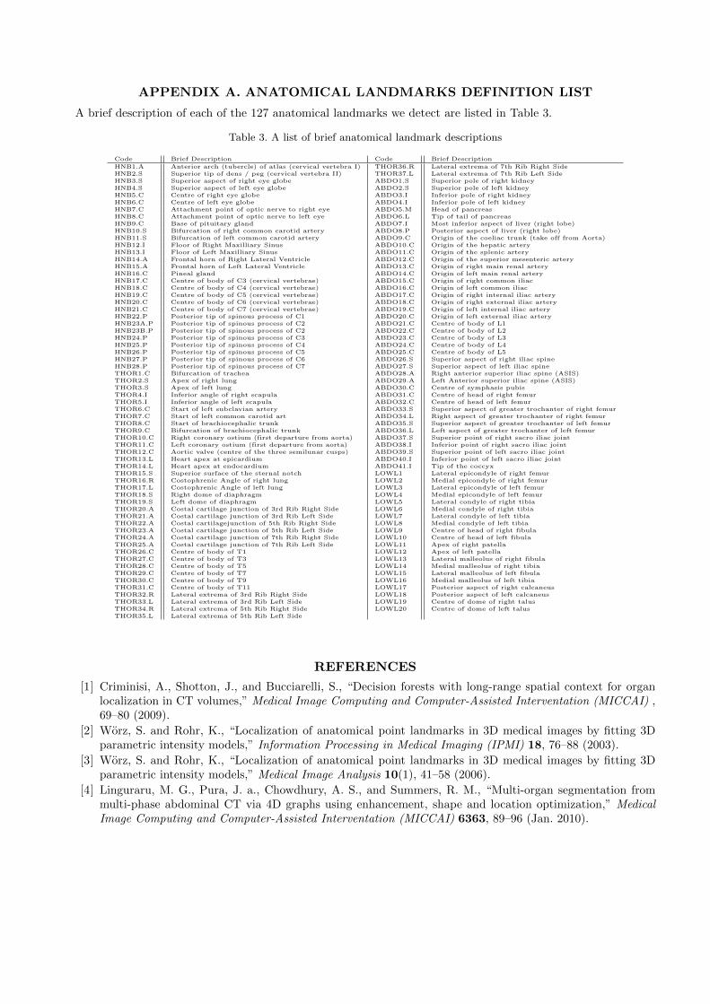
APPENDIX A. ANATOMICAL LANDMARKS DEFINITION LIST

A brief description of each of the 127 anatomical landmarks we detect are listed in Table 3.

Table 3. A list of brief anatomical landmark descriptions

Code Brief Description Code Brief Description

HNB1.A Anterior arch (tubercle) of atlas (cervical vertebra I) THOR36.R Lateral extrema of 7th Rib Right SideHNB2.S Superior tip of dens / peg (cervical vertebra II) THOR37.L Lateral extrema of 7th Rib Left SideHNB3.S Superior aspect of right eye globe ABDO1.S Superior pole of right kidneyHNB4.S Superior aspect of left eye globe ABDO2.S Superior pole of left kidneyHNB5.C Centre of right eye globe ABDO3.I Inferior pole of right kidneyHNB6.C Centre of left eye globe ABDO4.I Inferior pole of left kidneyHNB7.C Attachment point of optic nerve to right eye ABDO5.M Head of pancreasHNB8.C Attachment point of optic nerve to left eye ABDO6.L Tip of tail of pancreasHNB9.C Base of pituitary gland ABDO7.I Most inferior aspect of liver (right lobe)HNB10.S Bifurcation of right common carotid artery ABDO8.P Posterior aspect of liver (right lobe)HNB11.S Bifurcation of left common carotid artery ABDO9.C Origin of the coeliac trunk (take off from Aorta)HNB12.I Floor of Right Maxilliary Sinus ABDO10.C Origin of the hepatic arteryHNB13.I Floor of Left Maxilliary Sinus ABDO11.C Origin of the splenic arteryHNB14.A Frontal horn of Right Lateral Ventricle ABDO12.C Origin of the superior mesenteric arteryHNB15.A Frontal horn of Left Lateral Ventricle ABDO13.C Origin of right main renal arteryHNB16.C Pineal gland ABDO14.C Origin of left main renal arteryHNB17.C Centre of body of C3 (cervical vertebrae) ABDO15.C Origin of right common iliacHNB18.C Centre of body of C4 (cervical vertebrae) ABDO16.C Origin of left common iliacHNB19.C Centre of body of C5 (cervical vertebrae) ABDO17.C Origin of right internal iliac arteryHNB20.C Centre of body of C6 (cervical vertebrae) ABDO18.C Origin of right external iliac arteryHNB21.C Centre of body of C7 (cervical vertebrae) ABDO19.C Origin of left internal iliac arteryHNB22.P Posterior tip of spinous process of C1 ABDO20.C Origin of left external iliac arteryHNB23A.P Posterior tip of spinous process of C2 ABDO21.C Centre of body of L1HNB23B.P Posterior tip of spinous process of C2 ABDO22.C Centre of body of L2HNB24.P Posterior tip of spinous process of C3 ABDO23.C Centre of body of L3HNB25.P Posterior tip of spinous process of C4 ABDO24.C Centre of body of L4HNB26.P Posterior tip of spinous process of C5 ABDO25.C Centre of body of L5HNB27.P Posterior tip of spinous process of C6 ABDO26.S Superior aspect of right iliac spineHNB28.P Posterior tip of spinous process of C7 ABDO27.S Superior aspect of left iliac spineTHOR1.C Bifurcation of trachea ABDO28.A Right anterior superior iliac spine (ASIS)THOR2.S Apex of right lung ABDO29.A Left Anterior superior iliac spine (ASIS)THOR3.S Apex of left lung ABDO30.C Centre of symphasis pubisTHOR4.I Inferior angle of right scapula ABDO31.C Centre of head of right femurTHOR5.I Inferior angle of left scapula ABDO32.C Centre of head of left femurTHOR6.C Start of left subclavian artery ABDO33.S Superior aspect of greater trochanter of right femurTHOR7.C Start of left common carotid art ABDO34.L Right aspect of greater trochanter of right femurTHOR8.C Start of brachiocephalic trunk ABDO35.S Superior aspect of greater trochanter of left femurTHOR9.C Bifurcation of brachiocephalic trunk ABDO36.L Left aspect of greater trochanter of left femurTHOR10.C Right coronary ostium (first departure from aorta) ABDO37.S Superior point of right sacro iliac jointTHOR11.C Left coronary ostium (first departure from aorta) ABDO38.I Inferior point of right sacro iliac jointTHOR12.C Aortic valve (centre of the three semilunar cusps) ABDO39.S Superior point of left sacro iliac jointTHOR13.L Heart apex at epicardium ABDO40.I Inferior point of left sacro iliac jointTHOR14.L Heart apex at endocardium ABDO41.I Tip of the coccyxTHOR15.S Superior surface of the sternal notch LOWL1 Lateral epicondyle of right femurTHOR16.R Costophrenic Angle of right lung LOWL2 Medial epicondyle of right femurTHOR17.L Costophrenic Angle of left lung LOWL3 Lateral epicondyle of left femurTHOR18.S Right dome of diaphragm LOWL4 Medial epicondyle of left femurTHOR19.S Left dome of diaphragm LOWL5 Lateral condyle of right tibiaTHOR20.A Costal cartilage junction of 3rd Rib Right Side LOWL6 Medial condyle of right tibiaTHOR21.A Costal cartilage junction of 3rd Rib Left Side LOWL7 Lateral condyle of left tibiaTHOR22.A Costal cartilagejunction of 5th Rib Right Side LOWL8 Medial condyle of left tibiaTHOR23.A Costal cartilage junction of 5th Rib Left Side LOWL9 Centre of head of right fibulaTHOR24.A Costal cartilage junction of 7th Rib Right Side LOWL10 Centre of head of left fibulaTHOR25.A Costal cartilage junction of 7th Rib Left Side LOWL11 Apex of right patellaTHOR26.C Centre of body of T1 LOWL12 Apex of left patellaTHOR27.C Centre of body of T3 LOWL13 Lateral malleolus of right fibulaTHOR28.C Centre of body of T5 LOWL14 Medial malleolus of right tibiaTHOR29.C Centre of body of T7 LOWL15 Lateral malleolus of left fibulaTHOR30.C Centre of body of T9 LOWL16 Medial malleolus of left tibiaTHOR31.C Centre of body of T11 LOWL17 Posterior aspect of right calcaneusTHOR32.R Lateral extrema of 3rd Rib Right Side LOWL18 Posterior aspect of left calcaneusTHOR33.L Lateral extrema of 3rd Rib Left Side LOWL19 Centre of dome of right talusTHOR34.R Lateral extrema of 5th Rib Right Side LOWL20 Centre of dome of left talusTHOR35.L Lateral extrema of 5th Rib Left Side

REFERENCES

[1] Criminisi, A., Shotton, J., and Bucciarelli, S., “Decision forests with long-range spatial context for organlocalization in CT volumes,” Medical Image Computing and Computer-Assisted Interventation (MICCAI) ,69–80 (2009).

[2] Worz, S. and Rohr, K., “Localization of anatomical point landmarks in 3D medical images by fitting 3Dparametric intensity models,” Information Processing in Medical Imaging (IPMI) 18, 76–88 (2003).

[3] Worz, S. and Rohr, K., “Localization of anatomical point landmarks in 3D medical images by fitting 3Dparametric intensity models,” Medical Image Analysis 10(1), 41–58 (2006).

[4] Linguraru, M. G., Pura, J. a., Chowdhury, A. S., and Summers, R. M., “Multi-organ segmentation frommulti-phase abdominal CT via 4D graphs using enhancement, shape and location optimization,” MedicalImage Computing and Computer-Assisted Interventation (MICCAI) 6363, 89–96 (Jan. 2010).

[5] Shimizu, A., Ohno, R., Ikegami, T., Kobatake, H., Nawanob, S., and Smutek, D., “Simultaneous extractionof multiple organs from abdominal CT,” International Symposium on Future CAD (2005).

[6] Shimizu, A., Ohno, R., Ikegami, T., Kobatake, H., Nawano, S., and Smutek, D., “Segmentation of multipleorgans in non-contrast 3D abdominal CT images,” International Journal of Computer Assisted Radiologyand Surgery 2, 135–142 (Nov. 2007).

[7] Yao, C., Wada, T., Shimizu, A., Kobatake, H., and Nawano, S., “Probabilistic atlas-guided eigen-organmethod for simultaneous bounding box estimation of multiple organs in volumetric CT images,” MedicalImaging Technology 24(3), 191–200 (2006).

[8] Okada, T., Linguraru, M. G., Hori, M., Summers, R. M., Tomiyama, N., and Sato, Y., “Abdominal Multi-organ CT Segmentation Using Organ Correlation Graph and Prediction-Based Shape and Location Priors,”Medical image computing and computer-assisted intervention (MICCAI) 8151, 275–282 (2013).

[9] Chu, C., Oda, M., Kitasaka, T., Misawa, K., Fujiwara, M., Hayashi, Y., Nimura, Y., Rueckert, D., andMori, K., “Multi-organ Segmentation Based on Spatially-Divided Probabilistic Atlas from 3D AbdominalCT Images,” Medical image computing and computer-assisted intervention (MICCAI) 8150, 165–172 (2013).

[10] Criminisi, A., Shotton, J., Robertson, D., and Konukoglu, E., “Regression forests for efficient anatomy de-tection and localization in CT studies,” Medical Computer Vision. Recognition Techniques and Applicationsin Medical Imaging , 106–117 (2011).

[11] Iglesias, J. E., Konukoglu, E., Montillo, A., Tu, Z., and Criminisi, A., “Combining generative and dis-criminative models for semantic segmentation of CT scans via active learning.,” Information Processing inMedical Imaging 22, 25–36 (Jan. 2011).

[12] Montillo, A., Shotton, J., Winn, J., Iglesias, J. E., Metaxas, D., and Criminisi, A., “Entangled decisionforests and their application for semantic segmentation of CT images.,” Information Processing in MedicalImaging 22, 184–96 (Jan. 2011).

[13] Pauly, O., Glocker, B., Criminisi, A., Mateus, D., Moller, A. M., Nekolla, S., and Navab, N., “Fast multi-ple organ detection and localization in whole-body MR dixon sequences.,” Medical Image Computing andComputer-Assisted Interventation (MICCAI) 14, 239–247 (Jan. 2011).

[14] Kohlberger, T., Sofka, M., Zhang, J., Birkbeck, N., Wetzl, J., Kaftan, J., Declerck, J., and Zhou, S. K.,“Automatic Multi-organ Segmentation Using Learning-Based Segmentation and Level Set Optimization,”in [Medical Image Computing and Computer-Assisted Intervention (MICCAI) ], Fichtinger, G., Martel, A.,and Peters, T., eds., Lecture Notes in Computer Science 6893, 338–345, Springer (2011).

[15] Liu, D., Zhou, K. S., Bernhardt, D., and Comaniciu, D., “Search Strategies for Multiple Landmark Detectionby Submodular Maximization,” Computer Vision and Pattern Recognition (CVPR) , 2831–2838 (2010).

[16] Liu, D. and Zhou, S. K., “Anatomical Landmark Detection Using Nearest Neighbor Matching and Submod-ular Optimization,” Medical image computing and computer-assisted intervention (MICCAI) 7512, 393–401(2012).

[17] Lay, N., Birkbeck, N., Zhang, J., and Zhou, S., “Rapid Multi-organ Segmentation Using Context Integrationand Discriminative Models,” in [Information Processing in Medical Imaging ], Gee, J., Joshi, S., Pohl, K.,Wells, W., and Zollei, L., eds., Lecture Notes in Computer Science 7917, 450–462, Springer Berlin Heidelberg(2013).

[18] Potesil, V., Kadir, T., Platsch, G., and Brady, M., “Improved Anatomical Landmark Localization in MedicalImages Using Dense Matching of Graphical Models,” British Machine Vision Conference (BMVC) , 1–10(2010).

[19] Donner, R., Menze, B. H., Bischof, H., and Langs, G., “Global localization of 3D anatomical structures bypre-filtered Hough forests and discrete optimization.,” Medical Image Analysis 17, 1304–1314 (Dec. 2013).

[20] Quinlan, J. R., [C4.5: Programs for Machine Learning ], Morgan Kaufmann series in Machine Learning,Morgan Kaufmann (1993).