detecting anomalies in cellular networks using an … anomalies in cellular networks using an...

Detecting Anomalies in Cellular NetworksUsing an Ensemble Method

Gabriela F. Ciocarlie, Ulf LindqvistSRI International

Menlo Park, California, USA{gabriela.ciocarlie,ulf.lindqvist}@sri.com

Szabolcs NovaczkiNokia Siemens Networks Research

Budapest, [email protected]

Henning SanneckNokia Siemens Networks Research

Munich, [email protected]

Abstract—The Self-Organizing Networks (SON) concept in-cludes the functional area known as self-healing, which aimsto automate the detection and diagnosis of, and recovery from,network degradations and outages. This paper focuses on theproblem of cell anomaly detection, addressing partial and com-plete degradations in cell-service performance, and it proposes anadaptive ensemble method framework for modeling cell behavior.The framework uses Key Performance Indicators (KPIs) to deter-mine cell-performance status and is able to cope with legitimatesystem changes (i.e., concept drift). The results, generated usingreal cellular network data, suggest that the proposed ensemblemethod automatically and significantly improves the detectionquality over univariate and multivariate methods, while usingintrinsic system knowledge to enhance performance.

Index Terms—Self-Organizing Networks (SON), cell anomalydetection, Self-Healing, performance management, Key Perfor-mance Indicators

I. INTRODUCTION

The need for adaptive, self-organizing heterogeneous net-works is particularly apparent given the explosion of mobiledata traffic (Chapter 10 in [1]) that stems from increased use ofsmartphones, tablets, and netbooks for day-to-day tasks. Theexpectations for mobile networks have grown along with theirpopularity, and include ease of use, high-speed data transmis-sion, and responsiveness. Heterogeneous Networks (HetNet)combining different Radio Access Technologies (RATs) (3G,LTE, WiFi) and different cell layers (macro, micro, pico)within those RATs can offer these capabilities, providingvirtually unlimited capacity and ubiquitous coverage. How-ever, a high degree of distribution introduces a high levelof complexity requiring additional mechanisms, such as Self-Organizing Networks [1], to manage that complexity.

A. Self-Healing for SON

This paper focuses on self-healing capabilities, which re-duce operator effort and outage time, thereby providing fastermaintenance. Specifically, the problem that we address is auto-matic cell anomaly detection. Typically, research has focusedonly on Cell-Outage Detection (COD) [2] and Cell-OutageCompensation (COC) [3] concepts, but, more recently, detec-tion of general anomalies has also been addressed [4]. Thispaper addresses both the outage case and the case where thecell can provide a certain level of service, but its performancehas degraded to a point below an expected tolerable level anddirectly impacts users’ experience.

B. Contributions

The key challenge for addressing the more general problemof cell degradation is creating a robust method for modelingnormal cell behavior. This approach uses Key PerformanceIndicators (KPIs), which are highly dynamic measurements ofcell performance, to determine the state of a cell. KPIs requiremodeling techniques that can cope with concept drift, definedas the phenomenon where the normal behavior of the systemlegitimately changes over time (e.g., by the increasing amountof user-induced traffic demand).

This paper proposes a novel method for modeling cellbehavior to help address these problems. Our implementationand experiments focus on the problem of creating adaptivemodels, leveraging the intrinsic characteristics of the environ-ment where the models are created. The work described hereprovides several contributions by:

• proposing a new ensemble-method approach for cellanomaly detection that computes a numerical measurereferred to as the KPI degradation level [5], to indicatethe severity of the degradation,

• using intrinsic knowledge of the system to enhance theensemble-method learning in order to cope with conceptdrift and provide automation,

• building a system to implement the algorithms, applyingthe system to a real KPI dataset, and analyzing theperformance of the proposed framework.

II. CELL ANOMALY DETECTION

The first goal of the proposed framework is determiningthe relevant features needed for detecting anomalies in cellbehavior based on the KPI measurements. Because KPIs aremeasurements that are collected as ordered sequences of valuesof a variable at equally spaced time intervals, they constitutea time series and can be analyzed with known methods fortime-series analysis. An anomaly in a time series can be eithera single observation or a subsequence of a time series withrespect to a normal time series. Testing is defined as thecomparison of a set of KPI data to a model of the normal stateestablished by an earlier observed set of KPI data referred to astraining data. Ground truth is defined as the labels associatedwith the data points that indicate whether or not the datarepresents a real problem.

ISBN 978-3-901882-53-1, 9th CNSM and Workshops ©2013 IFIP. CNSM Short Paper171

Our hypothesis is that no single traditional time-seriesanomaly detection method (classifier) could provide the de-sired detection performance. This is due to the wide range inthe types of KPIs that need to be monitored, and the widerange of network incidents that need to be detected.

The proposed ensemble method combines different clas-sifiers and classifies new data points by taking a weightedvote of their prediction. It effectively creates a new compounddetection method that, with optimized weight parameter valueslearned by modeling the monitored data, can perform signifi-cantly better than any single method.

A. Univariate Time-Series Analysis

Individual KPIs collected for each cell are univariate timeseries that can be analyzed with the following methods:

• Using a sliding window, an Empirical Cumulative Dis-tribution Function (ECDF) [6] is computed for eachwindow. In the training phase, sliding windows that aresimilar based on the Kolmogorov-Smirnov (KS) test arecaptured in clusters represented by a centroid. In thetesting phase, each sliding window is tested against thecentroids of the clusters and KPI degradation level isdefined as the minimum distance from the centroids.

• A Support Vector Machine (SVM) [7] method is used tobuild KPI models. The training windows are used to buildone-class SVMs [8] with a radial basis function (RBF)kernel. In the testing phase, the anomaly score of a testwindow is 0 or 1, depending on whether it is classified asnormal (score of 0) or anomalous (score of 1). The KPIdegradation level is computed as the normalized value ofabnormal sequences in a number of consecutive tests.

• Using a predictive approach, KPI behavior is capturedby autoregressive, integrated moving average (ARIMA)models. Seasonal components are removed using STL,a Seasonal-Trend decomposition procedure based onLoess [9]. STL is robust to outliers, meaning that noisewill not affect the seasonal and the trend components, butonly the residual component. Two different implementa-tions of the ARIMA modeling are used: static “o,” inwhich only one model is created; and dynamic “m,” inwhich multiple models are created over time.

B. Multivariate Time-Series Analysis

The set of all KPIs collected for each cell is considered amultivariate time series that can be analyzed with the followingmethods:

• Using a sliding window, multivariate one-class SVMmodels are built across all time series. In the testingphase, their output is just a label with the value normalor abnormal. This approach provides a high-level viewof the KPIs’ behavior as a whole without providing aseverity indication for each KPI. This multivariate methodis relevant for the ensemble-method framework, in whichthe multivariate prediction is considered when generatingindividual KPI degradation levels.

• Using a predictive approach, Vector Auto-regressive(VAR) models are applied for the multivariate case. VARis a statistical model that generalizes the univariate ARmodel [10]. The VAR approach generates a model foreach KPI of a cell while capturing the linear interdepen-dencies among all KPIs (i.e., each KPI is expressed inrelationship to all the other KPIs). The VAR models en-able seasonal adjustment. Two different implementationsof the VAR modeling are used: static “o,” in which onlyone model is created; and dynamic “m,” in which multiplemodels are created over time.

The computation of KPI degradation levels for both mul-tivariate SVM and VAR models is analogous to the case ofunivariate ARIMA and SVM models.

C. Ensemble Method for Cell Anomaly Detection

The proposed ensemble-method framework applies individ-ual univariate and multivariate methods to the training KPIdata and relies on context information (available for cellu-lar networks) extracted from human-generated ConfigurationManagement (CM) or confirmed Fault Management (FM)input data to make informed decisions. Confirmed FM data isdefined as the machine-generated alarms that were confirmedby human operators.

M3!

Training KPI data for individual methods!

Generate models using univariate/multivariate methods!

Pool of models for the ensemble method!ω1! ω2! ωN!ω3! …..!

Test against all models in the pool!

KPI degradation level!

CM data !

Age out models based on their performance!

Confirmed FM data!Update weights!

Human expert knowledge!

KPI data under test !

Predictions of all models!

Compute KPI level based on predictions and weights!

Legend!data!method!

D1!

M1!

D2!

M2!

D3!

D4!

D5!

M4!

C1!

M5! C1!C3!

C2!

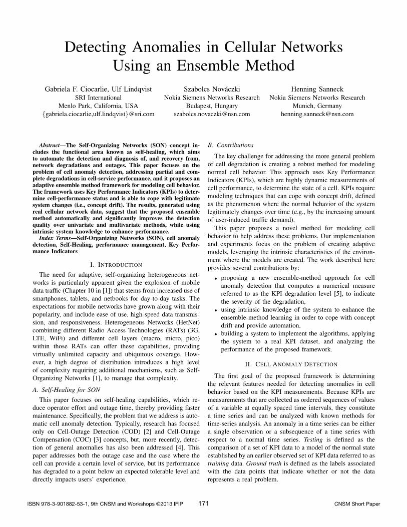
Fig. 1. Overall approach of the proposed ensemble method applied to asingle cell in a cellular network. Data is depicted in blue rectangles andmethods in pink rectangles with rounded corners. The remaining elementsindicate different context information. The dashed lines indicated that an eventis triggered in the presence of new evidence/data

Figure 1 presents the details of the proposed ensemblemethod, which implements a modified version of the weightedmajority algorithm (WMA) [11]. The modified WMA returnsa KPI degradation level in the range [0,1] and uses contextinformation for updating the weights and creating new models.

• Initially, for a given time period, the KPI measurementsof a given cell are selected as the training dataset (D1)for the pool of models of the ensemble method.


• A diverse set of univariate and multivariate algorithms(M1) is applied to the training dataset (D1).

• The result of (M1) is a set of models used as the poolof models for the ensemble method (D2). Each model inthe pool of models has a weight, ωi, associated with it.For the initial pool of models, all models have the sameweight value assigned (ωi = 1).

• Given the pool of models (D2), the stream of KPIs isused in a continuous fashion as the testing dataset (D5).Any CM change (C1) triggers the testing dataset to alsobecome the training KPI dataset, after which the methodfor generating a new set of models (M1) is executed.If the pool of models reaches the maximum number ofmodels, the CM change also triggers an exponential decayaging mechanism (M4), which removes models from thepool based on both their age and performance (accordingto ωi ∗ αagei , where 0 < α < 1 and agei is the numberof hours since the model was created).

• The testing dataset (D5) is tested against the models in thepool of models using the testing techniques correspondingto the univariate and multivariate methods (M2).

• The result of (M2) is a set of KPI-degradation-levelpredictions provided by each individual model in the poolof models (D3).Ground truth information updates (human-expert knowl-edge (C2), confirmed FM data (C3), and CM change in-formation (C1)) trigger the update weights method (M5),which penalizes the models in the pool of predictorsbased on their prediction with regards to the ground truth(ωi ← β∗ωi, where β ∈ [0, 1]). The human-expert knowl-edge assumes a manual process; while the confirmed FMdata usage and the CM change detection are automatedprocesses. The result of (M5) is an updated pool ofmodels (D2) with adjusted weights, which continue tobe used in the testing mode.

• All the predictions in (D3) along with the weights associ-ated with the corresponding models are used in a modifiedweighed majority approach (M3) to generate the KPIdegradation level, where τ ∈ [0, 1] is the threshold thatdetermines whether data is deemed normal or abnormal.

q0 =∑

KPI<τ

ωi, q1 =∑

KPI≥τωi

• The result of (M3) is the KPI degradation level (D4)associated with each KPI measurement of each cell.

KPI level =

∑KPI≥τ

ωi∗KPI leveli

∑KPI≥τ

ωi, if q1 > q0

∑KPI<τ

ωi∗KPI leveli

∑KPI<τ

ωi, if q1 ≤ q0

(1)

III. EVALUATION OF ENSEMBLE METHOD

This section quantifies the increase in detection accuracywhen the ensemble method is applied to the proposed uni-

!

th_perf&=&0.5&

86&0.

00.

20.

40.

60.

81.

0

Timekp

i_le

vels

●●●●●●●●●●●●●●●●●●●●●●●●●●●●●●●●●●●●●●●●●●●●●●●●●●●●●●

●●●●●●●●●●●●●●●●●●●●●●●●●●●●●●●●●●●●●●●●●●●●●●●●●●●●●●●●●●●●●●●●●●●●●●●●●●●●●●●●●●●●●●●●●●●●●●●●●●●●●●●●●●●●●●●●●●●●●●●●●●●●●●●●●●●●●●●●●●●●●●●●●●●●●●●●●●●●●●●●●●●●●●●●●●●●●●●●●●●●●●●●●●●●●●●●●●●●●●●●●●●●●●●●●●●●●●●●●●●●●●●●●●●●●●●●●●●●●●●●●●●●●●●●●●●●●●●●●●●●●●●●●●●●●●●●●●●●●●●●●●●●●●●●●●●●●●●●●●●●●●●●●●●●●●●●●●●●●●●●●●●●●●●●●●●●●●●●●●●●

●●●●●●●●●●●●●●●●●●●●●●●●●●●●●●●●●●●●●●●●●●●●●●●●●

●●●●●●

●●●●●●●●●●●●●●●●●●●●●●●●●●●●●●●●●●●●●●●●●●●●●●●●●●●●●●●●●●●●●●●●●●●●●●●●●●●●●●●●●●●●●●●●●●●●●●●●●●●●●●●●●●●●●●●●●●●●●●●●●●●●●●●●●●

●●●●●●●●●●●●●●●

●●●●●●●●●●●●●●●●●●●●●●●●●●●●●●●●●●●●●●●●●●●●●●●●●●●●●●●●●●●●●●●●●●●●●●●●●●●●●●●●●●●●●●●●●●●●●

●●●●●●●●●●●●●●●●●●

●●●●●●●●●●●●●●●●●●●●●●●●●●●●●●

●●

●●●●●●●●●●●●

●

●●●●●●●●●

●●

●●●●●●●●●●

●●●●●●●●●●●●●●●●●●●●●●●●●●●●●●

●●●●●●●●●●●●●●●●●●●●●

●

●●●●●●●●●●●●●●●●●●●●●●●●●●●●●●●●●●●●●●●●●●●●●●●●●●●●●●●●●●●●●●●●●●●●●●●●●●●●●●●●●●●●●●●●●●●●●●●●●●●●●●●●●●●●●●●●●●●●●●

●●●●●●●●●●●●●●●●

●●●●●●●●●●●●

●●●●●●●●●●●●●●●●●●●●●●●●●

●●●●●●●●●●●●●●●

●●●●●●●●●●●●●●●●●●●●

●●●●●●●●●●

●●●●●●●●●●●●●●●●●●●●●●●●●●●●●●●●●●●●●●●●

●●●●●

●●●●●●●●●●●

●●●●●●

●●●●

●

●●●

●●●●●●●●●●●●●●

●●●●●●●●●●●●●●●●●●●●●●●●

●●●●●●●●●●●●●●●●●●●●●●●●●●●●●●●●●●●●●●●●●●●●●●●●●●●●●●●●●

●●●●●●●●●●●●●●●●●●●●

●●●●●●●●●●●●●●●●●●●●●●●●●●●●●●●●●●●●●●●●●●●●●●●●●●●●●●●●●●●●●●●●●●●●●●●●●●●●●●●●●●●●●●●●●●●●●●●●●●●●●●●●●●●●●●●●●●●●●●●●●●●●●●●●●●●●●●●●●●●●●●●●●●●●●●●●●●●●●●●●●●●●●●●●●●●●●●●●●●●●●●●●●●●●●●●●●●●●●●●●●●●●●●●●●●●●●●●●●●●●●

●●●●●●●●●●●●●●●●●●●●●●●●●●●●●●●●●●●●●●●●●●●●●●●●●

●●●●●●●●●●●●●●●●●●●●●●●●●●●●●●●●●●●●●●●●●●●●●●●●●●●●●●●●●●●●●●●●●●●●●●●●●●●●●●●●●●●●●●●●●●●●●●●●●●●●●●●●●●●●●●●●●●●●●●●●●●●●●●●●●●●●●●●●●●●●●●●●●●●●●●●●●●●●●●●●●●●●●●●●●●●●●●●●●●●●●●●●●●●●●●●●●●●●●●●●●●●●●●●●●●●●●●●●●●●●●●●●●●●●●●●●●●●●●●●●●●●●●●●●●●●●●●●●●●●●●●●●●●●●●●●●●●●●●●●●●●●●●●●●●●●●●●●●●●●●●●●●●●●●●●●●●●●●●●●●●●●●●●●●●●●●●●●●●●●●●●●●●●●●●●●●●●●●●●●●●●●●●●●●●●●●●●●●●●●●●●●●●●●●●●●●●●●●●●●●●●●●●●●●●●●●●●●●●●●●●●●●●●●●●●●●●●●●●●●●●●●●●●●●●●●●●●●●●●●●●●●●●●●●●●●●●●●●●●●●●●●●●●●●●●●●●●●●●●●●●●●●●●●●●●●●●●●●●●●●●●●●●●●●●●●●●●●●●●●●●●●●●●●●●●●●●●●●●●●●●●●●●●●●●●●●●●●●●●●●●●●●●●●●●●●●●●●●●●●●●●●●●●●●●●●●●●●●●●●●●●●●●●●●●●●●●●●●●●●●●●●●●●●●●●●●●●●●●●●●●●●●●●●●●●●●●●●●●●●●●●●●●●●●●●●●●●●●●●●●●●●●●●●●●●●●●●●●●●●●●●●●●●●●●●●●●●●●●●●●●●●●●●●●●●●●●●●●●●●●●●●●●●●●●●●●●●●●●●●●●●●●●●●●●●●●●●●●●●●●●●●●●●●●●●●●●●●●●●●●●●●●●●●●●●●●●●●●●●●●●●●●●●●●●●●●●●●●●●●●●●●●●●●●●●●●●●●●●●●●●●●●●●●●●●●●●●●●●●●●●●●●●●●●●●●●●●●●●●●●●●●●●●●●●●●●●●●●●●●●●●●●●●●●●●●●●●●●●●●●●●●●●●●●●●●●●●●●●●●●●●●●●●●●●●●●●●●●●●●●●●●●●●●●●●●●●●●●●●●●●●●●●●●●●●●●●●●●●●●●●●●●●●●●●●●●●●●●●●●●●●●●●●●●●●●●●●●●●●●●●●●●●●●●●●●●●●●

●●●●●●●●●●●●●●●●●●●●●●●●●●●●●●●●●●●●●●●●●●●●●●●●●●●●●●●●●●●●●●●●●●●●●●●●●●●●●●●●●●●●●●●●●●●●●●●●●●●●●●●●●●●●●●●●●●●●●●●●●●●●●●●●●●●●●●●●●●●●●●●●●●●●●●●●●●●●●●●●●●●●●●●●●●●●●●●●●●●●●●●●●●●●●●●●●●●●●●●●●●●●●●●●●●●●●●●●●●●●●●●●●●●●●●●●●●●●●●●●●●●●●●●●●●●●●●●●●●●●●●●●●●●●●●●●●●●●●●●●●●●●●●●●●●●●●●●●●●●●●●●●●●●●●●●●●●●●●●●●●●●●●●●●●●●●●●●●●●●●●●●●●●●●●●●●●●●●●●●●●●●●●●●●●●●●●●●●●●●●●●●●●●●●●●●●●●●●●●●

●

●

ARIMA(912,24,m)ARIMA(912,24,o)ECDF(912,72,8)SVM(912,0.02)uSVM(912,24,0.01)VAR(912,24,m)VAR(912,24,o)mWMAGround Truth

Modified−WMA prediction

01/13/2012 01/27/2012 02/10/2012 02/24/2012 03/09/2012

Part 2 – Description of results

th_perf&=&0.5&

86&

0.0

0.2

0.4

0.6

0.8

1.0

Time

kpi_

leve

ls

●●●●●●●●●●●●●●●●●●●●●●●●●●●●●●●●●●●●●●●●●●●●●●●●●●●●●●

●●●●●●●●●●●●●●●●●●●●●●●●●●●●●●●●●●●●●●●●●●●●●●●●●●●●●●●●●●●●●●●●●●●●●●●●●●●●●●●●●●●●●●●●●●●●●●●●●●●●●●●●●●●●●●●●●●●●●●●●●●●●●●●●●●●●●●●●●●●●●●●●●●●●●●●●●●●●●●●●●●●●●●●●●●●●●●●●●●●●●●●●●●●●●●●●●●●●●●●●●●●●●●●●●●●●●●●●●●●●●●●●●●●●●●●●●●●●●●●●●●●●●●●●●●●●●●●●●●●●●●●●●●●●●●●●●●●●●●●●●●●●●●●●●●●●●●●●●●●●●●●●●●●●●●●●●●●●●●●●●●●●●●●●●●●●●●●●●●●●

●●●●●●●●●●●●●●●●●●●●●●●●●●●●●●●●●●●●●●●●●●●●●●●●●

●●●●●●

●●●●●●●●●●●●●●●●●●●●●●●●●●●●●●●●●●●●●●●●●●●●●●●●●●●●●●●●●●●●●●●●●●●●●●●●●●●●●●●●●●●●●●●●●●●●●●●●●●●●●●●●●●●●●●●●●●●●●●●●●●●●●●●●●●

●●●●●●●●●●●●●●●

●●●●●●●●●●●●●●●●●●●●●●●●●●●●●●●●●●●●●●●●●●●●●●●●●●●●●●●●●●●●●●●●●●●●●●●●●●●●●●●●●●●●●●●●●●●●●

●●●●●●●●●●●●●●●●●●

●●●●●●●●●●●●●●●●●●●●●●●●●●●●●●

●●

●●●●●●●●●●●●

●

●●●●●●●●●

●●

●●●●●●●●●●

●●●●●●●●●●●●●●●●●●●●●●●●●●●●●●

●●●●●●●●●●●●●●●●●●●●●

●

●●●●●●●●●●●●●●●●●●●●●●●●●●●●●●●●●●●●●●●●●●●●●●●●●●●●●●●●●●●●●●●●●●●●●●●●●●●●●●●●●●●●●●●●●●●●●●●●●●●●●●●●●●●●●●●●●●●●●●

●●●●●●●●●●●●●●●●

●●●●●●●●●●●●

●●●●●●●●●●●●●●●●●●●●●●●●●

●●●●●●●●●●●●●●●

●●●●●●●●●●●●●●●●●●●●

●●●●●●●●●●

●●●●●●●●●●●●●●●●●●●●●●●●●●●●●●●●●●●●●●●●

●●●●●

●●●●●●●●●●●

●●●●●●

●●●●

●

●●●

●●●●●●●●●●●●●●

●●●●●●●●●●●●●●●●●●●●●●●●

●●●●●●●●●●●●●●●●●●●●●●●●●●●●●●●●●●●●●●●●●●●●●●●●●●●●●●●●●

●●●●●●●●●●●●●●●●●●●●

●●●●●●●●●●●●●●●●●●●●●●●●●●●●●●●●●●●●●●●●●●●●●●●●●●●●●●●●●●●●●●●●●●●●●●●●●●●●●●●●●●●●●●●●●●●●●●●●●●●●●●●●●●●●●●●●●●●●●●●●●●●●●●●●●●●●●●●●●●●●●●●●●●●●●●●●●●●●●●●●●●●●●●●●●●●●●●●●●●●●●●●●●●●●●●●●●●●●●●●●●●●●●●●●●●●●●●●●●●●●●

●●●●●●●●●●●●●●●●●●●●●●●●●●●●●●●●●●●●●●●●●●●●●●●●●

●●●●●●●●●●●●●●●●●●●●●●●●●●●●●●●●●●●●●●●●●●●●●●●●●●●●●●●●●●●●●●●●●●●●●●●●●●●●●●●●●●●●●●●●●●●●●●●●●●●●●●●●●●●●●●●●●●●●●●●●●●●●●●●●●●●●●●●●●●●●●●●●●●●●●●●●●●●●●●●●●●●●●●●●●●●●●●●●●●●●●●●●●●●●●●●●●●●●●●●●●●●●●●●●●●●●●●●●●●●●●●●●●●●●●●●●●●●●●●●●●●●●●●●●●●●●●●●●●●●●●●●●●●●●●●●●●●●●●●●●●●●●●●●●●●●●●●●●●●●●●●●●●●●●●●●●●●●●●●●●●●●●●●●●●●●●●●●●●●●●●●●●●●●●●●●●●●●●●●●●●●●●●●●●●●●●●●●●●●●●●●●●●●●●●●●●●●●●●●●●●●●●●●●●●●●●●●●●●●●●●●●●●●●●●●●●●●●●●●●●●●●●●●●●●●●●●●●●●●●●●●●●●●●●●●●●●●●●●●●●●●●●●●●●●●●●●●●●●●●●●●●●●●●●●●●●●●●●●●●●●●●●●●●●●●●●●●●●●●●●●●●●●●●●●●●●●●●●●●●●●●●●●●●●●●●●●●●●●●●●●●●●●●●●●●●●●●●●●●●●●●●●●●●●●●●●●●●●●●●●●●●●●●●●●●●●●●●●●●●●●●●●●●●●●●●●●●●●●●●●●●●●●●●●●●●●●●●●●●●●●●●●●●●●●●●●●●●●●●●●●●●●●●●●●●●●●●●●●●●●●●●●●●●●●●●●●●●●●●●●●●●●●●●●●●●●●●●●●●●●●●●●●●●●●●●●●●●●●●●●●●●●●●●●●●●●●●●●●●●●●●●●●●●●●●●●●●●●●●●●●●●●●●●●●●●●●●●●●●●●●●●●●●●●●●●●●●●●●●●●●●●●●●●●●●●●●●●●●●●●●●●●●●●●●●●●●●●●●●●●●●●●●●●●●●●●●●●●●●●●●●●●●●●●●●●●●●●●●●●●●●●●●●●●●●●●●●●●●●●●●●●●●●●●●●●●●●●●●●●●●●●●●●●●●●●●●●●●●●●●●●●●●●●●●●●●●●●●●●●●●●●●●●●●●●●●●●●●●●●●●●●●●●●●●●●●●●●●●●●●●●●●●●●●●●●●●●●●●●●●●●●●●●●●●●●●●●●

●●●●●●●●●●●●●●●●●●●●●●●●●●●●●●●●●●●●●●●●●●●●●●●●●●●●●●●●●●●●●●●●●●●●●●●●●●●●●●●●●●●●●●●●●●●●●●●●●●●●●●●●●●●●●●●●●●●●●●●●●●●●●●●●●●●●●●●●●●●●●●●●●●●●●●●●●●●●●●●●●●●●●●●●●●●●●●●●●●●●●●●●●●●●●●●●●●●●●●●●●●●●●●●●●●●●●●●●●●●●●●●●●●●●●●●●●●●●●●●●●●●●●●●●●●●●●●●●●●●●●●●●●●●●●●●●●●●●●●●●●●●●●●●●●●●●●●●●●●●●●●●●●●●●●●●●●●●●●●●●●●●●●●●●●●●●●●●●●●●●●●●●●●●●●●●●●●●●●●●●●●●●●●●●●●●●●●●●●●●●●●●●●●●●●●●●●●●●●●●

●

●



01/13/2012 01/27/2012 02/10/2012 02/24/2012 03/09/2012


!

th_perf&=&0.5&

86&

0.0

0.2

0.4

0.6

0.8

1.0

Time

kpi_

leve

ls●●●●●●●●●●●●●●●●●●●●●●●●●●●●●●●●●●●●●●●●●●●●●●●●●●●●●●

●●●●●●●●●●●●●●●●●●●●●●●●●●●●●●●●●●●●●●●●●●●●●●●●●●●●●●●●●●●●●●●●●●●●●●●●●●●●●●●●●●●●●●●●●●●●●●●●●●●●●●●●●●●●●●●●●●●●●●●●●●●●●●●●●●●●●●●●●●●●●●●●●●●●●●●●●●●●●●●●●●●●●●●●●●●●●●●●●●●●●●●●●●●●●●●●●●●●●●●●●●●●●●●●●●●●●●●●●●●●●●●●●●●●●●●●●●●●●●●●●●●●●●●●●●●●●●●●●●●●●●●●●●●●●●●●●●●●●●●●●●●●●●●●●●●●●●●●●●●●●●●●●●●●●●●●●●●●●●●●●●●●●●●●●●●●●●●●●●●●

●●●●●●●●●●●●●●●●●●●●●●●●●●●●●●●●●●●●●●●●●●●●●●●●●

●●●●●●

●●●●●●●●●●●●●●●●●●●●●●●●●●●●●●●●●●●●●●●●●●●●●●●●●●●●●●●●●●●●●●●●●●●●●●●●●●●●●●●●●●●●●●●●●●●●●●●●●●●●●●●●●●●●●●●●●●●●●●●●●●●●●●●●●●

●●●●●●●●●●●●●●●

●●●●●●●●●●●●●●●●●●●●●●●●●●●●●●●●●●●●●●●●●●●●●●●●●●●●●●●●●●●●●●●●●●●●●●●●●●●●●●●●●●●●●●●●●●●●●

●●●●●●●●●●●●●●●●●●

●●●●●●●●●●●●●●●●●●●●●●●●●●●●●●

●●

●●●●●●●●●●●●

●

●●●●●●●●●

●●

●●●●●●●●●●

●●●●●●●●●●●●●●●●●●●●●●●●●●●●●●

●●●●●●●●●●●●●●●●●●●●●

●

●●●●●●●●●●●●●●●●●●●●●●●●●●●●●●●●●●●●●●●●●●●●●●●●●●●●●●●●●●●●●●●●●●●●●●●●●●●●●●●●●●●●●●●●●●●●●●●●●●●●●●●●●●●●●●●●●●●●●●

●●●●●●●●●●●●●●●●

●●●●●●●●●●●●

●●●●●●●●●●●●●●●●●●●●●●●●●

●●●●●●●●●●●●●●●

●●●●●●●●●●●●●●●●●●●●

●●●●●●●●●●

●●●●●●●●●●●●●●●●●●●●●●●●●●●●●●●●●●●●●●●●

●●●●●

●●●●●●●●●●●

●●●●●●

●●●●

●

●●●

●●●●●●●●●●●●●●

●●●●●●●●●●●●●●●●●●●●●●●●

●●●●●●●●●●●●●●●●●●●●●●●●●●●●●●●●●●●●●●●●●●●●●●●●●●●●●●●●●

●●●●●●●●●●●●●●●●●●●●

●●●●●●●●●●●●●●●●●●●●●●●●●●●●●●●●●●●●●●●●●●●●●●●●●●●●●●●●●●●●●●●●●●●●●●●●●●●●●●●●●●●●●●●●●●●●●●●●●●●●●●●●●●●●●●●●●●●●●●●●●●●●●●●●●●●●●●●●●●●●●●●●●●●●●●●●●●●●●●●●●●●●●●●●●●●●●●●●●●●●●●●●●●●●●●●●●●●●●●●●●●●●●●●●●●●●●●●●●●●●●

●●●●●●●●●●●●●●●●●●●●●●●●●●●●●●●●●●●●●●●●●●●●●●●●●

●●●●●●●●●●●●●●●●●●●●●●●●●●●●●●●●●●●●●●●●●●●●●●●●●●●●●●●●●●●●●●●●●●●●●●●●●●●●●●●●●●●●●●●●●●●●●●●●●●●●●●●●●●●●●●●●●●●●●●●●●●●●●●●●●●●●●●●●●●●●●●●●●●●●●●●●●●●●●●●●●●●●●●●●●●●●●●●●●●●●●●●●●●●●●●●●●●●●●●●●●●●●●●●●●●●●●●●●●●●●●●●●●●●●●●●●●●●●●●●●●●●●●●●●●●●●●●●●●●●●●●●●●●●●●●●●●●●●●●●●●●●●●●●●●●●●●●●●●●●●●●●●●●●●●●●●●●●●●●●●●●●●●●●●●●●●●●●●●●●●●●●●●●●●●●●●●●●●●●●●●●●●●●●●●●●●●●●●●●●●●●●●●●●●●●●●●●●●●●●●●●●●●●●●●●●●●●●●●●●●●●●●●●●●●●●●●●●●●●●●●●●●●●●●●●●●●●●●●●●●●●●●●●●●●●●●●●●●●●●●●●●●●●●●●●●●●●●●●●●●●●●●●●●●●●●●●●●●●●●●●●●●●●●●●●●●●●●●●●●●●●●●●●●●●●●●●●●●●●●●●●●●●●●●●●●●●●●●●●●●●●●●●●●●●●●●●●●●●●●●●●●●●●●●●●●●●●●●●●●●●●●●●●●●●●●●●●●●●●●●●●●●●●●●●●●●●●●●●●●●●●●●●●●●●●●●●●●●●●●●●●●●●●●●●●●●●●●●●●●●●●●●●●●●●●●●●●●●●●●●●●●●●●●●●●●●●●●●●●●●●●●●●●●●●●●●●●●●●●●●●●●●●●●●●●●●●●●●●●●●●●●●●●●●●●●●●●●●●●●●●●●●●●●●●●●●●●●●●●●●●●●●●●●●●●●●●●●●●●●●●●●●●●●●●●●●●●●●●●●●●●●●●●●●●●●●●●●●●●●●●●●●●●●●●●●●●●●●●●●●●●●●●●●●●●●●●●●●●●●●●●●●●●●●●●●●●●●●●●●●●●●●●●●●●●●●●●●●●●●●●●●●●●●●●●●●●●●●●●●●●●●●●●●●●●●●●●●●●●●●●●●●●●●●●●●●●●●●●●●●●●●●●●●●●●●●●●●●●●●●●●●●●●●●●●●●●●●●●●●●●●●●●●●●●●●●●●●●●●●●●●●●●●●●●●●●●●●

●●●●●●●●●●●●●●●●●●●●●●●●●●●●●●●●●●●●●●●●●●●●●●●●●●●●●●●●●●●●●●●●●●●●●●●●●●●●●●●●●●●●●●●●●●●●●●●●●●●●●●●●●●●●●●●●●●●●●●●●●●●●●●●●●●●●●●●●●●●●●●●●●●●●●●●●●●●●●●●●●●●●●●●●●●●●●●●●●●●●●●●●●●●●●●●●●●●●●●●●●●●●●●●●●●●●●●●●●●●●●●●●●●●●●●●●●●●●●●●●●●●●●●●●●●●●●●●●●●●●●●●●●●●●●●●●●●●●●●●●●●●●●●●●●●●●●●●●●●●●●●●●●●●●●●●●●●●●●●●●●●●●●●●●●●●●●●●●●●●●●●●●●●●●●●●●●●●●●●●●●●●●●●●●●●●●●●●●●●●●●●●●●●●●●●●●●●●●●●●

●

●



01/13/2012 01/27/2012 02/10/2012 02/24/2012 03/09/2012


th_perf&=&0.5&

86&

0.0

0.2

0.4

0.6

0.8

1.0

Time

kpi_

leve

ls

●●●●●●●●●●●●●●●●●●●●●●●●●●●●●●●●●●●●●●●●●●●●●●●●●●●●●●

●●●●●●●●●●●●●●●●●●●●●●●●●●●●●●●●●●●●●●●●●●●●●●●●●●●●●●●●●●●●●●●●●●●●●●●●●●●●●●●●●●●●●●●●●●●●●●●●●●●●●●●●●●●●●●●●●●●●●●●●●●●●●●●●●●●●●●●●●●●●●●●●●●●●●●●●●●●●●●●●●●●●●●●●●●●●●●●●●●●●●●●●●●●●●●●●●●●●●●●●●●●●●●●●●●●●●●●●●●●●●●●●●●●●●●●●●●●●●●●●●●●●●●●●●●●●●●●●●●●●●●●●●●●●●●●●●●●●●●●●●●●●●●●●●●●●●●●●●●●●●●●●●●●●●●●●●●●●●●●●●●●●●●●●●●●●●●●●●●●●

●●●●●●●●●●●●●●●●●●●●●●●●●●●●●●●●●●●●●●●●●●●●●●●●●

●●●●●●

●●●●●●●●●●●●●●●●●●●●●●●●●●●●●●●●●●●●●●●●●●●●●●●●●●●●●●●●●●●●●●●●●●●●●●●●●●●●●●●●●●●●●●●●●●●●●●●●●●●●●●●●●●●●●●●●●●●●●●●●●●●●●●●●●●

●●●●●●●●●●●●●●●

●●●●●●●●●●●●●●●●●●●●●●●●●●●●●●●●●●●●●●●●●●●●●●●●●●●●●●●●●●●●●●●●●●●●●●●●●●●●●●●●●●●●●●●●●●●●●

●●●●●●●●●●●●●●●●●●

●●●●●●●●●●●●●●●●●●●●●●●●●●●●●●

●●

●●●●●●●●●●●●

●

●●●●●●●●●

●●

●●●●●●●●●●

●●●●●●●●●●●●●●●●●●●●●●●●●●●●●●

●●●●●●●●●●●●●●●●●●●●●

●

●●●●●●●●●●●●●●●●●●●●●●●●●●●●●●●●●●●●●●●●●●●●●●●●●●●●●●●●●●●●●●●●●●●●●●●●●●●●●●●●●●●●●●●●●●●●●●●●●●●●●●●●●●●●●●●●●●●●●●

●●●●●●●●●●●●●●●●

●●●●●●●●●●●●

●●●●●●●●●●●●●●●●●●●●●●●●●

●●●●●●●●●●●●●●●

●●●●●●●●●●●●●●●●●●●●

●●●●●●●●●●

●●●●●●●●●●●●●●●●●●●●●●●●●●●●●●●●●●●●●●●●

●●●●●

●●●●●●●●●●●

●●●●●●

●●●●

●

●●●

●●●●●●●●●●●●●●

●●●●●●●●●●●●●●●●●●●●●●●●

●●●●●●●●●●●●●●●●●●●●●●●●●●●●●●●●●●●●●●●●●●●●●●●●●●●●●●●●●

●●●●●●●●●●●●●●●●●●●●

●●●●●●●●●●●●●●●●●●●●●●●●●●●●●●●●●●●●●●●●●●●●●●●●●●●●●●●●●●●●●●●●●●●●●●●●●●●●●●●●●●●●●●●●●●●●●●●●●●●●●●●●●●●●●●●●●●●●●●●●●●●●●●●●●●●●●●●●●●●●●●●●●●●●●●●●●●●●●●●●●●●●●●●●●●●●●●●●●●●●●●●●●●●●●●●●●●●●●●●●●●●●●●●●●●●●●●●●●●●●●

●●●●●●●●●●●●●●●●●●●●●●●●●●●●●●●●●●●●●●●●●●●●●●●●●

●●●●●●●●●●●●●●●●●●●●●●●●●●●●●●●●●●●●●●●●●●●●●●●●●●●●●●●●●●●●●●●●●●●●●●●●●●●●●●●●●●●●●●●●●●●●●●●●●●●●●●●●●●●●●●●●●●●●●●●●●●●●●●●●●●●●●●●●●●●●●●●●●●●●●●●●●●●●●●●●●●●●●●●●●●●●●●●●●●●●●●●●●●●●●●●●●●●●●●●●●●●●●●●●●●●●●●●●●●●●●●●●●●●●●●●●●●●●●●●●●●●●●●●●●●●●●●●●●●●●●●●●●●●●●●●●●●●●●●●●●●●●●●●●●●●●●●●●●●●●●●●●●●●●●●●●●●●●●●●●●●●●●●●●●●●●●●●●●●●●●●●●●●●●●●●●●●●●●●●●●●●●●●●●●●●●●●●●●●●●●●●●●●●●●●●●●●●●●●●●●●●●●●●●●●●●●●●●●●●●●●●●●●●●●●●●●●●●●●●●●●●●●●●●●●●●●●●●●●●●●●●●●●●●●●●●●●●●●●●●●●●●●●●●●●●●●●●●●●●●●●●●●●●●●●●●●●●●●●●●●●●●●●●●●●●●●●●●●●●●●●●●●●●●●●●●●●●●●●●●●●●●●●●●●●●●●●●●●●●●●●●●●●●●●●●●●●●●●●●●●●●●●●●●●●●●●●●●●●●●●●●●●●●●●●●●●●●●●●●●●●●●●●●●●●●●●●●●●●●●●●●●●●●●●●●●●●●●●●●●●●●●●●●●●●●●●●●●●●●●●●●●●●●●●●●●●●●●●●●●●●●●●●●●●●●●●●●●●●●●●●●●●●●●●●●●●●●●●●●●●●●●●●●●●●●●●●●●●●●●●●●●●●●●●●●●●●●●●●●●●●●●●●●●●●●●●●●●●●●●●●●●●●●●●●●●●●●●●●●●●●●●●●●●●●●●●●●●●●●●●●●●●●●●●●●●●●●●●●●●●●●●●●●●●●●●●●●●●●●●●●●●●●●●●●●●●●●●●●●●●●●●●●●●●●●●●●●●●●●●●●●●●●●●●●●●●●●●●●●●●●●●●●●●●●●●●●●●●●●●●●●●●●●●●●●●●●●●●●●●●●●●●●●●●●●●●●●●●●●●●●●●●●●●●●●●●●●●●●●●●●●●●●●●●●●●●●●●●●●●●●●●●●●●●●●●●●●●●●●●●●●●●●●●●●●●●●●

●●●●●●●●●●●●●●●●●●●●●●●●●●●●●●●●●●●●●●●●●●●●●●●●●●●●●●●●●●●●●●●●●●●●●●●●●●●●●●●●●●●●●●●●●●●●●●●●●●●●●●●●●●●●●●●●●●●●●●●●●●●●●●●●●●●●●●●●●●●●●●●●●●●●●●●●●●●●●●●●●●●●●●●●●●●●●●●●●●●●●●●●●●●●●●●●●●●●●●●●●●●●●●●●●●●●●●●●●●●●●●●●●●●●●●●●●●●●●●●●●●●●●●●●●●●●●●●●●●●●●●●●●●●●●●●●●●●●●●●●●●●●●●●●●●●●●●●●●●●●●●●●●●●●●●●●●●●●●●●●●●●●●●●●●●●●●●●●●●●●●●●●●●●●●●●●●●●●●●●●●●●●●●●●●●●●●●●●●●●●●●●●●●●●●●●●●●●●●●●

●

●



01/13/2012 01/27/2012 02/10/2012 02/24/2012 03/09/2012


ARIMA_m'ARIMA_o'ECDF'SVM'uSVM'VAR_m'VAR_o'mWMA'Ground'Truth'

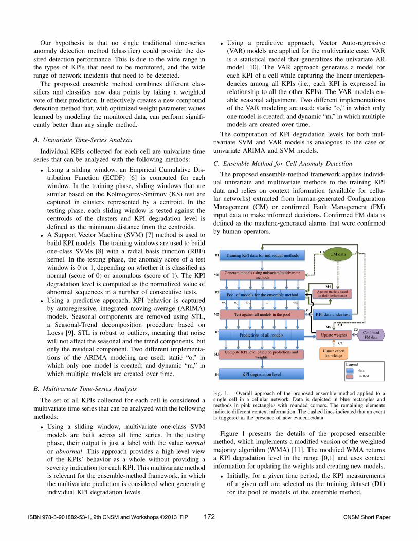
Fig. 2. The output KPI degradation levels generated by the ensemble methodfor a given cell and call control KPI are marked with blue circles, while redrepresents the manually generated labels. The remaining series represent theKPI degradation levels generated by the univariate and multivariate methods(τ = 0.5 and β = 0.8)

variate and multivariate methods. The experimental corpusconsisted of a KPI dataset containing data from 70 cells ofa live mobile network. For each cell, 12 KPIs were collectedevery hour for four months, from 11/15/2011 to 03/19/2012.The KPIs have different characteristics; some of them, such asdownlink or uplink data volume or throughput, are measure-ments of user traffic utilization; while others, such as drop-callrate and successful call-setup rate, are measurements of callcontrol parameters.

The experimental dataset had no associated ground truth.To address this limitation, labels were manually generated toindicate whether the data represented a real problem or not,based on engineering knowledge applied to KPI-data visualinspection.

The pool of models was trained on the first 912 hoursof data, and the ensemble method was trained on the next500 hours). The remainder of the dataset was used to makethe ensemble prediction based on the learned weights. Theparameters were set to τ = 0.5 and β = 0.8.

Figure 2 presents the KPI degradation levels generated bythe ensemble methods (modified WMA depicted as mWMA)as well as the univariate and multivariate methods.

The two metrics used for the performance evaluation were:

• False Positive Rate (FPR) defined as the percentage ofnormal data deemed as abnormal by the detector

• Detection Rate (DR) defined as the percentage of abnor-mal data deemed as abnormal by the detector.

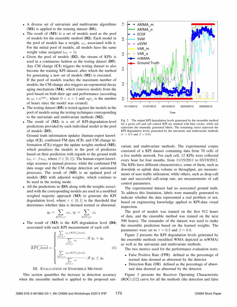
Figure 3 presents the Receiver Operating Characteristic(ROC) [12] curve for all the methods (the detection and false


●

●

●●●●

●

0 20 40 60 80 100

020

4060

8010

0

Average false positive rate [%]

Aver

age

dete

ctio

n ra

te [%

]●

●

●

●

●●

●

●

●

ARIMA(912,24,m)ARIMA(912,24,o)ECDF(912,72,8)SVM(912,0.02)uSVM(912,24,0.01)VAR(912,24,m)VAR(912,24,o)mWMA

!

="0.5"

• Using a predictive approach, we apply Vector Auto-regressive (VAR) models for the multivariate case. VARis a statistical model used to capture the linear interde-pendencies among multiple time series, generalizing theunivariate AR model [7]. The VAR approach generatesa model for each KPI of a cell, while capturing thelinear interdependencies among all KPIs (i.e., each KPIis expressed in relationship to all the other KPIs). TheVAR models allow for seasonal adjustment.


C. Ensemble Method for Cell Degradation Detection

Our proposed ensemble method framework applies individ-ual univariate and multivariate methods to the training KPIdata leading to the construction of a pool of different pre-dictors. Using the pool of predictors, the predictions obtainedon the KPI data under test (i.e., being subject to detection)along with the weights allocated to each predictor lead to thecomputation of the KPI degradation level (i.e., the deviationof a KPI from its normal state). The proposed methodsrely on context information (available for cellular networks)extracted from human-generated, Configuration Management(CM) or confirmed Fault Management (FM) input data tomake informed decisions. We define confirmed FM data asthe machine-generated alarms that were confirmed by humanoperators.

Figure 2 presents the details of the proposed ensemblemethod, where we distinguish between data, methods, contextinformation and human expert knowledge. Each cell is char-acterized by a set of KPI measurements generated as a streamof data. The ensemble method is applied to each cell. Theproposed ensemble method implements a modified version ofthe weighted majority algorithm (WMA) [8] that returns aKPI degradation level in the range [0,1] and uses the contextinformation for updating the weights and creating new models.

• Initially, for a given period of time, the KPI measurementsof a given cell are selected as the training dataset (D1)for the pool of models of the ensemble method.

• A diverse set of univariate and multivariate algorithms(M1) is applied to the training dataset (D1). The univari-ate methods operate at the individual KPI degradationlevel, while the multivariate methods operate across allKPIs.

• The result of (M1) is a set of models used as the poolof models for the ensemble method (D2). Each model inthe pool of models has a weight, !i, associated with it.For the initial pool of models, all models have the sameweight value assigned (!i = 1).

• Given the pool of models (D2), the stream of KPIs isused in a continuous fashion as the testing dataset (D5).

– Any CM change (C1) triggers the testing dataset toalso become the training KPI dataset, after whichthe method for generating a new set of models

(M1) is executed. The CM change is determinedautomatically, based on the state of CM data.

– If the pool of models reaches the maximum num-ber of models, the CM change also triggers anexponential decay aging mechanism (M4), whichremoves models from the pool based on both theirage and performance (according to !i ⇤↵agei , where↵ 2 [0, 1] and agei is the number of hours since themodel was created).


• The result of (M2) is a set of KPI degradation levelpredictions provided by each individual model in the poolof models (D3). Some of the predictions are binary (a KPIdegradation level of 0 represents normal and 1 representsabnormal) and some have continuous values in the [0, 1]range.

– Ground truth information updates (human expertknowledge (C2), confirmed FM data (C3) and cellclassification based on CM information (D6)) trig-gers the update weights method (M5), which pe-nalizes the models in the pool of predictors basedon their prediction with regards to the ground truth(!i � ⇤ !i, where � 2 [0, 1]). The human expertknowledge assumes a manual process, while the con-firmed FM data usage and outlier detection appliedto CM homogenous cells are automated processes.

• Based on CM data (C1), an outlier detection algorithm(M6) is applied to cells with identical configurations.The assumption is that CM homogenous cells (i.e., cellswith identical/very similar configuration) should exhibitthe same behavior across all KPIs. This component takesinto consideration the behavior across multiple cells.

• The result of (M6) indicates whether the cell under testis considered an outlier or not (D6) with respect to cellswith homogenous configurations.

– The result of (M5) is an updated pool of models (D2)with adjusted weights, which continue to be used inthe testing mode.

• All the predictions in (D3) along with the weights associ-ated with the corresponding models are used in a modifiedweighed majority approach (M3) to generate the KPIdegradation level, where ⌧ 2 [0, 1] is the threshold thatdetermines whether data is deemed normal or abnormal.

q0 =X

KPI<⌧

!i, q1 =X

KPI�⌧

!i

The ⌧ value is not dependent on any KPI semantic andcan be tuned based on the oprational environment. Con-sequently, for a small oprations team a higher threasholdwould trigger less alerts, while for a larger operationsteam a lower threashold would trigger more alerts.

• The result of (M3) is the KPI degradation level (D4)

●

●

●●●●

●

0 20 40 60 80 100

020

4060

8010

0

Average false positive rate [%]

Aver

age

dete

ctio

n ra

te [%

]●

●

●

●

●●

●

●

●

ARIMA(912,24,m)ARIMA(912,24,o)ECDF(912,72,8)SVM(912,0.02)uSVM(912,24,0.01)VAR(912,24,m)VAR(912,24,o)mWMA

!

="0.5"

• Using a predictive approach, we apply Vector Auto-regressive (VAR) models for the multivariate case. VARis a statistical model used to capture the linear interde-pendencies among multiple time series, generalizing theunivariate AR model [7]. The VAR approach generatesa model for each KPI of a cell, while capturing thelinear interdependencies among all KPIs (i.e., each KPIis expressed in relationship to all the other KPIs). TheVAR models allow for seasonal adjustment.


C. Ensemble Method for Cell Degradation Detection

Our proposed ensemble method framework applies individ-ual univariate and multivariate methods to the training KPIdata leading to the construction of a pool of different pre-dictors. Using the pool of predictors, the predictions obtainedon the KPI data under test (i.e., being subject to detection)along with the weights allocated to each predictor lead to thecomputation of the KPI degradation level (i.e., the deviationof a KPI from its normal state). The proposed methodsrely on context information (available for cellular networks)extracted from human-generated, Configuration Management(CM) or confirmed Fault Management (FM) input data tomake informed decisions. We define confirmed FM data asthe machine-generated alarms that were confirmed by humanoperators.

Figure 2 presents the details of the proposed ensemblemethod, where we distinguish between data, methods, contextinformation and human expert knowledge. Each cell is char-acterized by a set of KPI measurements generated as a streamof data. The ensemble method is applied to each cell. Theproposed ensemble method implements a modified version ofthe weighted majority algorithm (WMA) [8] that returns aKPI degradation level in the range [0,1] and uses the contextinformation for updating the weights and creating new models.

• Initially, for a given period of time, the KPI measurementsof a given cell are selected as the training dataset (D1)for the pool of models of the ensemble method.

• A diverse set of univariate and multivariate algorithms(M1) is applied to the training dataset (D1). The univari-ate methods operate at the individual KPI degradationlevel, while the multivariate methods operate across allKPIs.

• The result of (M1) is a set of models used as the poolof models for the ensemble method (D2). Each model inthe pool of models has a weight, !i, associated with it.For the initial pool of models, all models have the sameweight value assigned (!i = 1).

• Given the pool of models (D2), the stream of KPIs isused in a continuous fashion as the testing dataset (D5).

– Any CM change (C1) triggers the testing dataset toalso become the training KPI dataset, after whichthe method for generating a new set of models

(M1) is executed. The CM change is determinedautomatically, based on the state of CM data.

– If the pool of models reaches the maximum num-ber of models, the CM change also triggers anexponential decay aging mechanism (M4), whichremoves models from the pool based on both theirage and performance (according to !i ⇤↵agei , where↵ 2 [0, 1] and agei is the number of hours since themodel was created).


• The result of (M2) is a set of KPI degradation levelpredictions provided by each individual model in the poolof models (D3). Some of the predictions are binary (a KPIdegradation level of 0 represents normal and 1 representsabnormal) and some have continuous values in the [0, 1]range.

– Ground truth information updates (human expertknowledge (C2), confirmed FM data (C3) and cellclassification based on CM information (D6)) trig-gers the update weights method (M5), which pe-nalizes the models in the pool of predictors basedon their prediction with regards to the ground truth(!i � ⇤ !i, where � 2 [0, 1]). The human expertknowledge assumes a manual process, while the con-firmed FM data usage and outlier detection appliedto CM homogenous cells are automated processes.

• Based on CM data (C1), an outlier detection algorithm(M6) is applied to cells with identical configurations.The assumption is that CM homogenous cells (i.e., cellswith identical/very similar configuration) should exhibitthe same behavior across all KPIs. This component takesinto consideration the behavior across multiple cells.

• The result of (M6) indicates whether the cell under testis considered an outlier or not (D6) with respect to cellswith homogenous configurations.

– The result of (M5) is an updated pool of models (D2)with adjusted weights, which continue to be used inthe testing mode.

• All the predictions in (D3) along with the weights associ-ated with the corresponding models are used in a modifiedweighed majority approach (M3) to generate the KPIdegradation level, where ⌧ 2 [0, 1] is the threshold thatdetermines whether data is deemed normal or abnormal.

q0 =X

KPI<⌧

!i, q1 =X

KPI�⌧

!i

The ⌧ value is not dependent on any KPI semantic andcan be tuned based on the oprational environment. Con-sequently, for a small oprations team a higher threasholdwould trigger less alerts, while for a larger operationsteam a lower threashold would trigger more alerts.

• The result of (M3) is the KPI degradation level (D4)

ARIMA_m'ARIMA_o'ECDF'SVM'uSVM'VAR_m'VAR_o'mWMA'

Fig. 3. ROC curves for all individual methods and the ensemble method

positive rates were computed as an average across all the70 cells analyzed) and it illustrates well that the ensemblemethod (mWMA) exhibits the best performance, confirmingour hypothesis.

IV. RELATED WORK

The proposed framework aims to detect partial and completedegradations in cell-service performance. Previous researchaddressed the cell-outage detection [2] and cell-outage com-pensation [3] concepts. For the problem of cell-outage detec-tion, Mueller et al. [2] proposed a detection mechanism thatuses Neighbor Cell List (NCL) reports. Compared to our work,Muller’s approach was limited to only catatonic-cell detection,while not every isolated node reflected an outage situation.

Another approach for estimating failures in cellular net-works was proposed by Coluccia et al. [13] to analyze eventsat different levels: transmission of IP packets, transport andapplication layer communication establishment, user levelsession activation, and control-plane procedures.

D’Alconzo et al. [14] proposed an anomaly detection algo-rithm for 3G cellular networks that detects events that mightput the stability and performance of the network at risk.

More recently, detection of general anomalies has also beenaddressed [4], [5], [6]. However, to the best of our knowledge,our approach is the first to employ an adaptive ensemblemethod that copes with concept drift.

V. CONCLUSIONS AND FUTURE WORK

This paper proposed a novel ensemble method for modelingcell behavior that builds adaptive models and uses the intrinsiccharacteristics of the environment where the models are cre-ated to improve its performance. The design was implementedand applied to a dataset consisting of KPI data collected from areal operational cell network. The experimental results indicate

that our system provides significant detection performanceimprovements over stand-alone univariate and multivariatemethods.

We are currently planning experimental evaluation of ourcell anomaly detection method in a network operator setting.Additional work is needed to integrate our detection com-ponent with a diagnosis engine that combines the detectoroutput with other information sources to assist operators indetermining the cause of a detected anomaly. These results alsoserve as the foundation for research in other areas of networkoperation, specifically to evaluate the impact of configurationchanges on critical measures of network performance.

ACKNOWLEDGMENT

We thank Lauri Oksanen, Kari Aaltonen, Richard Fehlmann,Christoph Frenzel, Peter Szilagyi, Michael Freed, Ken Nitz,and Christopher Connolly for their contributions.

REFERENCES

[1] S. Hamalainen, H. Sanneck, and C. Sartori (eds.), “LTE Self-OrganizingNetworks (SON): Network Management Automation for OperationalEfficiency,” Wiley, 2012.

[2] C. M. Mueller, M. Kaschub, C. Blankenhorn, and S. Wanke, “A Cell Out-age Detection Algorithm Using Neighbor Cell List Reports,” InternationalWorkshop on Self-Organizing Systems, 2008.

[3] M. Amirijoo, L. Jorguseski, R. Litjens, and L.C. Schmelz, “Cell OutageCompensation in LTE Networks: Algorithms and Performance Assess-ment,” 2011 IEEE 73rd Vehicular Technology Conference (VTC Spring),15–18 May 2011.

[4] A. Bouillard, A. Junier and B. Ronot, “Hidden Anomaly Detection inTelecommunication Networks,” International Conference on Network andService Management (CNSM), Las Vegas, NV, October 2012.

[5] P. Szilagyi and S. Novaczki, “An Automatic Detection and DiagnosisFramework For Mobile Communication Systems,” IEEE Transactions onNetwork and Service Management, 2012.

[6] S. Novaczki, “An Improved Anomaly Detection and Diagnosis Frame-work for Mobile Network Operators,” 9th International Conference onDesign of Reliable Communication Networks (DRCN 2013), Budapest,March 2013.

[7] S. Ruping, “SVM Kernels for Time Series Analysis,” In R. Klinkenberget al. (eds.), LLWA 01 - Tagungsband der GI-Workshop-Woche Lernen- Lehren - Wissen - Adaptivitat, Forschungsberichte des FachbereichsInformatik der Universitat Dortmund, pp. 43-50, Dortmund, Germany,2001.

[8] J. Ma and S. Perkins, “Time-Series Novelty Detection Using One-ClassSupport Vector Machines,” Neural Networks, 2003.

[9] R. B. Cleveland, W. S. Cleveland, J. E. McRae, and I. Terpenning, “STL:A Seasonal-Trend Decomposition Procedure Based on Loess,” Journal ofOfficial Statistics, Vol. 6, No. 1, 1990.

[10] B. Pfaff, “VAR, SVAR and SVEC Models: Implementation Within RPackage vars,” Journal of Statistical Software, Vol. 27, Issue 4, 2008.

[11] N. Littlestone and M.K. Warmuth, “The Weighted Majority Algorithm,”Inf. Comput. 108, 2, 1994.

[12] D. M. Green and J. A. Swets, Signal Detection Theory and Psy-chophysics. New York, NY: John Wiley and Sons Inc. ISBN 0-471-32420-5, 1966.

[13] A. Coluccia, F. Ricciato, and P. Romirer-Maierhofer, “Bayesian Estima-tion of Network-Wide Mean Failure Probability in 3G Cellular Networks,”In PERFORM, Vol. 6821, Springer (2010), pp. 167-178.

[14] A. D’Alconzo, A. Coluccia, F. Ricciato, and P. Romirer-Maierhofer, “ADistribution-Based Approach to Anomaly Detection and Application to3G Mobile Traffic,” Global Telecommunications Conference (GLOBE-COM) 2009.


detecting anomalies in cellular networks using an … anomalies in cellular networks using an...

Documents