Designing Partial Differential Equations for ImageProcessing by Combining Differential Invariants∗

Zhouchen Lin1† Wei Zhang2 Xiaoou Tang2

1Microsoft Research Asia, zhoulin@microsoft.com2The Chinese University of Hong Kong, {zw007,xtang}@ie.cuhk.edu.hk

Abstract

Partial differential equations (PDEs) have been successful for solving many prob-lems in image processing and computer vision. However, designing PDEs usually re-quires high mathematical skills and good insight to the problems. In this paper, wepropose a framework for learning a system of PDEs from real data. Compared to thetraditional approaches to designing PDEs, our framework requires much less human in-telligence. We assume that the system consists of two PDEs. One controls the evolutionof the output and the other is for an indicator function that helps collect global infor-mation. As the PDEs should be shift and rotationally invariant, they must be functionsof differential invariants that are shift and rotationally invariant. Currently, we assumethat the PDEs are simply linear combinations of the fundamental differential invariantsup to second order. The combination coefficients can be learnt from real data via anoptimal control technique. The exemplary experiments show that the PDEs, designed inour unified way, can solve some image processing problems reasonably well. Hence ourframework is very promising. We expect that with future improvements our frameworkcould work for more image processing/computer vision problems.

1 Introduction

The applications of partial differential equations (PDEs) to computer vision and image pro-

cessing date back to the 1960s [9, 12]. However, this technique did not draw much attention

until the introduction of the concept of scale space by Koenderink [14] and Witkin [29] in

the 1980s. Perona and Malik’s work on anisotropic diffusion [23] further drew great inter-

est from researchers towards PDE-based methods. Nowadays, PDEs have been successfully

applied to many problems in image processing and computer vision [11, 8, 25, 2, 7], e.g.,∗Microsoft technical report #MSR-TR-2009-192. Patent filed.†Corresponding author.

1

denoising [23], enhancement [20], inpainting [4], segmentation [15], stereo and optical flow

computation.

In general, there are three kinds of methods used to design PDEs. For the first kind of

methods, PDEs are written down directly, based on some mathematical understandings on

the properties of the PDEs (e.g., anisotropic diffusion [23], shock filter [20] and curve evolu-

tion based equations [11, 25, 2, 7]). The second kind of methods basically define an energy

functional first, which collects the wish list of the desired properties of the output image,

and then derives the evolution equations by computing the Euler-Lagrange equation of the

energy functional (e.g., chapter 9 of [11]). The third kind of methods are axiomatic ap-

proaches, which first prescribe the properties, i.e., axioms, that the PDEs should hold and

then deduce the form of PDEs from these axioms (e.g., Alvarez et al.’s axiomatic formula-

tion of the scale-space theory [1]). All of these methods require both good insight to what

properties to hold and high mathematical skills, in order to acquire the desired PDEs. These

greatly limit the applications of PDEs to wider and more complex scopes. This motivates us

to explore whether there is an easier way of designing PDEs.

In this paper, we show that learning PDEs from given input-output sample image pairs

might be a possible way to designing PDEs in a lazy manner. The key idea is to assume

that the PDEs in sought could be written as combinations of “atoms” called fundamental

differential invariants. Then the problem boils down to determining the combination coef-

ficients among such “atoms”. This can be achieved by employing the technique of optimal

control governed by PDEs [17], where the objective functional is to minimize the difference

between the expected outputs (ground truth) and the actual outputs of the PDEs, given the

input images. Such input-output image pairs are provided by the user as training samples. As

a preliminary investigation, we assume that the system consists of two PDEs. One controls

the evolution of the output and the other is for an indicator function that helps collect global

information. As the PDEs should be shift and rotationally invariant, they must be functions

of fundamental differential invariants [19]. Currently, we only consider the case that the

PDEs are linear combinations of fundamental differential invariants up to second order, and

2

the objective functional simply utilizes the L2 norm to measure the output error.

Differential invariants are already widely used in computer vision and image processing.

However, the existing use of differential invariants is mainly limited to feature representation,

detection and matching [18]. Anisotropic PDE-based filtering of images [7, 8, 25] also uses

differential invariants. However, those PDEs are for image denoising and enhancement only,

and the deduction of affine and perspective differential invariants therein is rather involved.

Although our differential invariants are much simpler, we can obtain PDEs that are applicable

to more image processing problems.

The optimal control technique has also been applied to some computer vision and image

processing problems. In [13], Kimia et al. showed how to use this technique to solve energy

functionals arising from various problems, including shape evolution, morphology, optical

flow estimation and shape from shading, whose variables are governed by (partial) differen-

tial equations. Papadakis et al. also applied the optimal control technique extensively (e.g.,

optical flow estimation [22] and tracking [21]). Our framework is different from the exist-

ing work in that it is to determine the (coefficients in) PDEs, while the existing work is to

determine PDE outputs, in which the PDE is known.

We have to emphasize that we do not claim that our current framework, in its preliminary

form, can produce PDEs for all image processing/computer vision problems. However, we

show that it does work for some image processing problems: it produces PDEs that perform

reasonably well for these problems. The merit of our framework is that the PDEs are acquired

using the same mechanism. The only differences are in the sets of training images that

the user has to prepare and the computed combination coefficients among the fundamental

differential invariants. We do find problems that the current framework fails. Nonetheless,

the successful examples encourage us to further improve our framework in the future so that

it can handle more problems systematically.

The rest of this paper is organized as follows. In Section 2, we present our framework of

learning PDEs. In Section 3, we testify to the effectiveness of our framework by applying it

to five basic image processing problems. Then we conclude our paper in Section 4.

3

Table 1: Notationsx (x, y), spatial variable t temporal variableΩ an open region of R2 ∂Ω boundary of ΩQ Ω× (0, T ) Γ ∂Ω× (0, T )∇f gradient of f Hf Hessian of f⟨f⟩ {f, fx, fy, fxx, fxy, fyy, ⋅ ⋅ ⋅ }, i.e., the set of partial derivatives

of f up to an appropriate order, where fx = ∂f/∂x, etc.

2 Designing PDEs by Combining Differential Invariants

Now we present our framework of learning a PDE system from training sample images.

We assume that the PDE system consists of two PDEs. One is for the evolution of the

output image O, and the other is for the evolution of an indicator function ½. The goal

of introducing the indicator function is to collect large scale information in the image so

that the evolution of O can be correctly guided. Although the introduction of the indicator

function is inspired by the edge indicator in [11] (page 193), it may not necessarily be related

to the edge information for non-edge-detection problems. We assume the PDEs to be of

evolutionary type because a usual information process should consist of some (unknown)

steps. The time-dependent operations of the evolutionary PDEs resemble the different steps

of the information process. Moreover, for stationary PDEs it is not natural to define their

inputs and outputs, and the existence of their solutions is much less optimistic. So our PDE

system can be written as:⎧⎨⎩

∂O

∂t= LO(a, ⟨O⟩, ⟨½⟩), (x, t) ∈ Q,

O = 0, (x, t) ∈ Γ,O∣t=0 = O0, x ∈ Ω;

∂½

∂t= L½(b, ⟨½⟩, ⟨O⟩), (x, t) ∈ Q,

½ = 0, (x, t) ∈ Γ,½∣t=0 = ½0, x ∈ Ω.

(1)

The notations in the above equations can be found in Table 1, where Ω is the rectangular

region occupied by the input image I and T is the time that the PDE system finishes the

processing and outputs the results. For computational issues and ease of mathematical de-

duction, I will be padded with zeros of several pixels width around it. As we can change the

4

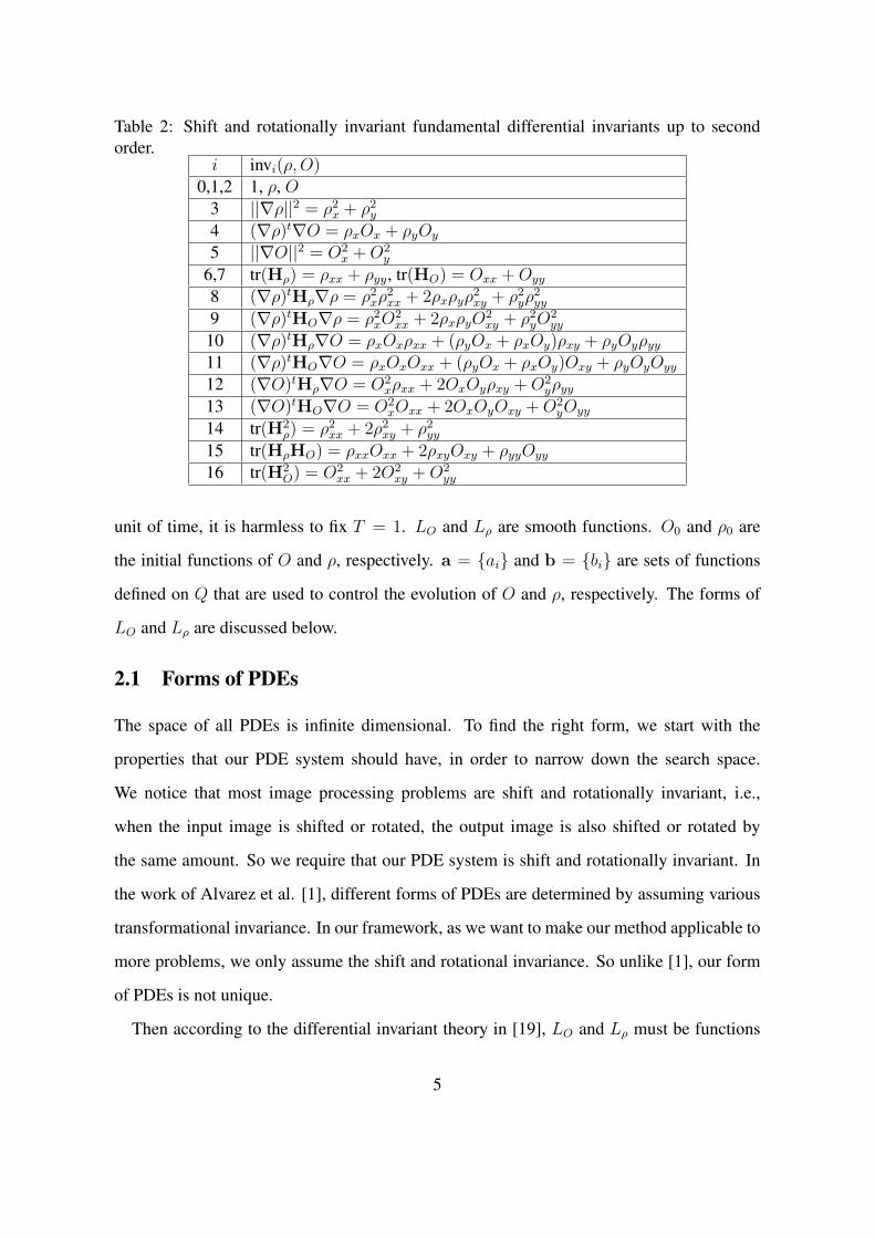
Table 2: Shift and rotationally invariant fundamental differential invariants up to secondorder.

i invi(½,O)0,1,2 1, ½, O

3 ∣∣∇½∣∣2 = ½2x + ½2y4 (∇½)t∇O = ½xOx + ½yOy

5 ∣∣∇O∣∣2 = O2x +O2

y

6,7 tr(H½) = ½xx + ½yy, tr(HO) = Oxx +Oyy

8 (∇½)tH½∇½ = ½2x½2xx + 2½x½y½

2xy + ½2y½

2yy

9 (∇½)tHO∇½ = ½2xO2xx + 2½x½yO

2xy + ½2yO

2yy

10 (∇½)tH½∇O = ½xOx½xx + (½yOx + ½xOy)½xy + ½yOy½yy11 (∇½)tHO∇O = ½xOxOxx + (½yOx + ½xOy)Oxy + ½yOyOyy

12 (∇O)tH½∇O = O2x½xx + 2OxOy½xy +O2

y½yy13 (∇O)tHO∇O = O2

xOxx + 2OxOyOxy +O2yOyy

14 tr(H2½) = ½2xx + 2½2xy + ½2yy

15 tr(H½HO) = ½xxOxx + 2½xyOxy + ½yyOyy

16 tr(H2O) = O2

xx + 2O2xy +O2

yy

unit of time, it is harmless to fix T = 1. LO and L½ are smooth functions. O0 and ½0 are

the initial functions of O and ½, respectively. a = {ai} and b = {bi} are sets of functions

defined on Q that are used to control the evolution of O and ½, respectively. The forms of

LO and L½ are discussed below.

2.1 Forms of PDEs

The space of all PDEs is infinite dimensional. To find the right form, we start with the

properties that our PDE system should have, in order to narrow down the search space.

We notice that most image processing problems are shift and rotationally invariant, i.e.,

when the input image is shifted or rotated, the output image is also shifted or rotated by

the same amount. So we require that our PDE system is shift and rotationally invariant. In

the work of Alvarez et al. [1], different forms of PDEs are determined by assuming various

transformational invariance. In our framework, as we want to make our method applicable to

more problems, we only assume the shift and rotational invariance. So unlike [1], our form

of PDEs is not unique.

Then according to the differential invariant theory in [19], LO and L½ must be functions

5

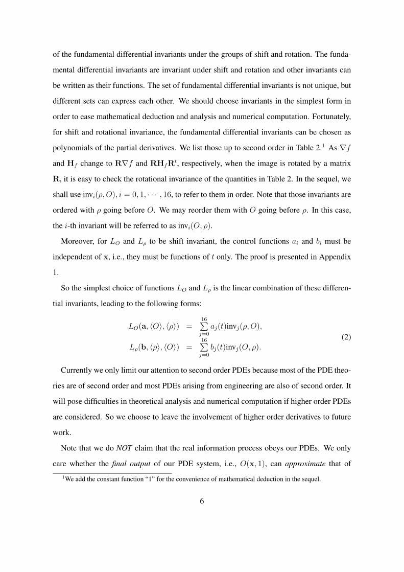
of the fundamental differential invariants under the groups of shift and rotation. The funda-

mental differential invariants are invariant under shift and rotation and other invariants can

be written as their functions. The set of fundamental differential invariants is not unique, but

different sets can express each other. We should choose invariants in the simplest form in

order to ease mathematical deduction and analysis and numerical computation. Fortunately,

for shift and rotational invariance, the fundamental differential invariants can be chosen as

polynomials of the partial derivatives. We list those up to second order in Table 2.1 As ∇f

and Hf change to R∇f and RHfRt, respectively, when the image is rotated by a matrix

R, it is easy to check the rotational invariance of the quantities in Table 2. In the sequel, we

shall use invi(½,O), i = 0, 1, ⋅ ⋅ ⋅ , 16, to refer to them in order. Note that those invariants are

ordered with ½ going before O. We may reorder them with O going before ½. In this case,

the i-th invariant will be referred to as invi(O, ½).

Moreover, for LO and L½ to be shift invariant, the control functions ai and bi must be

independent of x, i.e., they must be functions of t only. The proof is presented in Appendix

1.

So the simplest choice of functions LO and L½ is the linear combination of these differen-

tial invariants, leading to the following forms:

LO(a, ⟨O⟩, ⟨½⟩) =16∑j=0

aj(t)invj(½,O),

L½(b, ⟨½⟩, ⟨O⟩) =16∑j=0

bj(t)invj(O, ½).(2)

Currently we only limit our attention to second order PDEs because most of the PDE theo-

ries are of second order and most PDEs arising from engineering are also of second order. It

will pose difficulties in theoretical analysis and numerical computation if higher order PDEs

are considered. So we choose to leave the involvement of higher order derivatives to future

work.

Note that we do NOT claim that the real information process obeys our PDEs. We only

care whether the final output of our PDE system, i.e., O(x, 1), can approximate that of

1We add the constant function “1” for the convenience of mathematical deduction in the sequel.

6

the real process. For example, although O1(x, t) = ∥x∥2 sin t and O2(x, t) = (∥x∥2 + (1−t)∥x∥)(sin t+ t(1− t)∥x∥3) are very different functions, they initiate from the same function

at t = 0 and also settle down at the same function at time t = 1. So both functions fit our

purpose and we need not care whether the real process obeys either function.

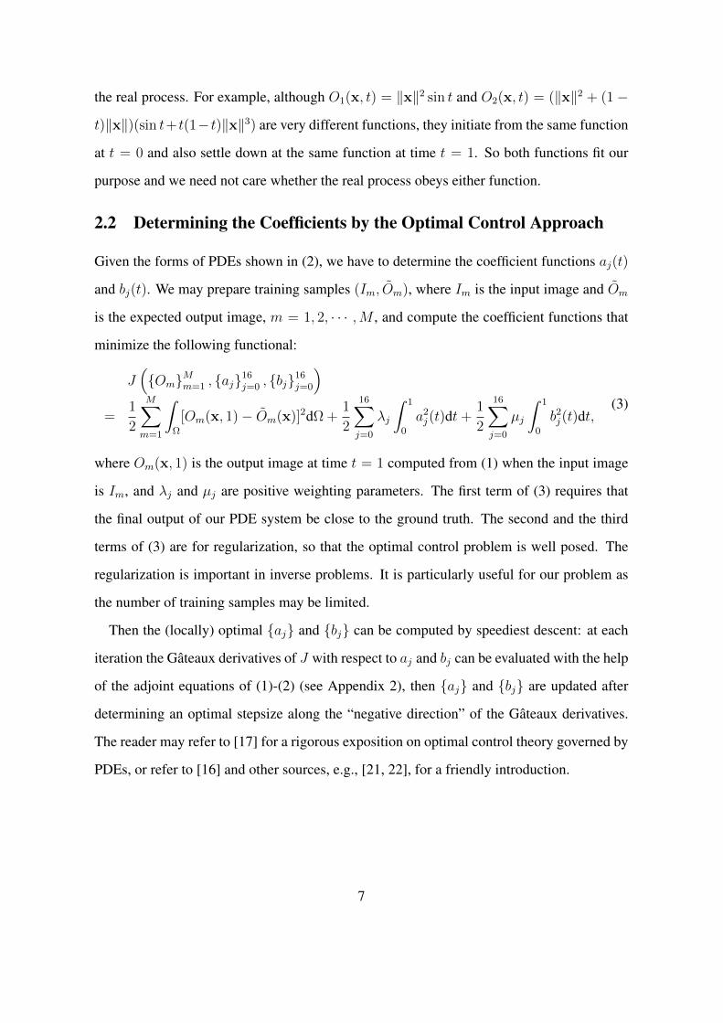
2.2 Determining the Coefficients by the Optimal Control Approach

Given the forms of PDEs shown in (2), we have to determine the coefficient functions aj(t)

and bj(t). We may prepare training samples (Im, Om), where Im is the input image and Om

is the expected output image, m = 1, 2, ⋅ ⋅ ⋅ ,M , and compute the coefficient functions that

minimize the following functional:

J({Om}Mm=1 , {aj}16j=0 , {bj}16j=0

)

=1

2

M∑m=1

∫

Ω

[Om(x, 1)− Om(x)]2dΩ +

1

2

16∑j=0

¸j

∫ 1

0

a2j(t)dt+1

2

16∑j=0

¹j

∫ 1

0

b2j(t)dt,(3)

where Om(x, 1) is the output image at time t = 1 computed from (1) when the input image

is Im, and ¸j and ¹j are positive weighting parameters. The first term of (3) requires that

the final output of our PDE system be close to the ground truth. The second and the third

terms of (3) are for regularization, so that the optimal control problem is well posed. The

regularization is important in inverse problems. It is particularly useful for our problem as

the number of training samples may be limited.

Then the (locally) optimal {aj} and {bj} can be computed by speediest descent: at each

iteration the Gateaux derivatives of J with respect to aj and bj can be evaluated with the help

of the adjoint equations of (1)-(2) (see Appendix 2), then {aj} and {bj} are updated after

determining an optimal stepsize along the “negative direction” of the Gateaux derivatives.

The reader may refer to [17] for a rigorous exposition on optimal control theory governed by

PDEs, or refer to [16] and other sources, e.g., [21, 22], for a friendly introduction.

7

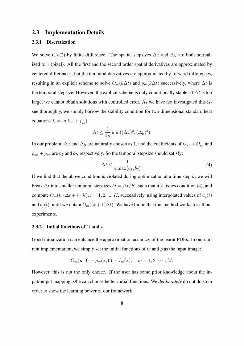
2.3 Implementation Details2.3.1 Discretization

We solve (1)-(2) by finite difference. The spatial stepsizes Δx and Δy are both normal-

ized to 1 (pixel). All the first and the second order spatial derivatives are approximated by

centered differences, but the temporal derivatives are approximated by forward differences,

resulting in an explicit scheme to solve Om(kΔt) and ½m(kΔt) successively, where Δt is

the temporal stepsize. However, the explicit scheme is only conditionally stable: if Δt is too

large, we cannot obtain solutions with controlled error. As we have not investigated this is-

sue thoroughly, we simply borrow the stability condition for two-dimensional standard heat

equations ft = ·(fxx + fyy):

Δt ≤ 1

4·min((Δx)2, (Δy)2).

In our problem, Δx and Δy are naturally chosen as 1, and the coefficients of Oxx +Oyy and

½xx + ½yy are a7 and b7, respectively. So the temporal stepsize should satisfy:

Δt ≤ 1

4max(a7, b7). (4)

If we find that the above condition is violated during optimization at a time step k, we will

break Δt into smaller temporal stepsizes ±t = Δt/K, such that it satisfies condition (4), and

compute Om(k ⋅Δt+ i ⋅ ±t), i = 1, 2, ..., K, successively, using interpolated values of aj(t)

and bj(t), until we obtain Om((k + 1)Δt). We have found that this method works for all our

experiments.

2.3.2 Initial functions of O and ½

Good initialization can enhance the approximation accuracy of the learnt PDEs. In our cur-

rent implementation, we simply set the initial functions of O and ½ as the input image:

Om(x, 0) = ½m(x, 0) = Im(x), m = 1, 2, ⋅ ⋅ ⋅ ,M.

However, this is not the only choice. If the user has some prior knowledge about the in-

put/output mapping, s/he can choose better initial functions. We deliberately do not do so in

order to show the learning power of our framework.

8

2.3.3 Initialization of {ai} and {bi}

We initialize {ai(t)} successively in time while fixing bi(t) ≡ 0, i = 0, 1, ⋅ ⋅ ⋅ , 16. At the first

time step, without any prior information, Om(Δt) is expected to be ΔtOm+(1−Δt)Om(0).

So ∂Om/∂t∣t=Δt is expected to be Om−O0 and we may solve {ai(0)} such that the difference

s({ai(0)}) ≡ 1

2

M∑m=1

∫

Ω

[16∑j=0

aj(0)invj(½m(0), Om(0)))− (Om −O0)

]2

dΩ

between the left and the right hand sides of (1) is minimized, where the integration here

should be understood as summation. After solving {ai(0)}, we can have Om(Δt) by solving

(1) at t = Δt. Suppose at the (k+1)-th step, we have solved Om(kΔt), then we may expect

that Om((k+ 1)Δt) = Δt1−kΔt

Om + (1−kΔt)−Δt1−kΔt

Om(kΔt) so that Om((k+ 1)Δt) could move

directly towards Om. So ∂Om/∂t∣t=(k+1)Δt is expected to be 11−kΔt

[Om − Om(kΔt)] and

{ai(kΔt)} can be solved in the same manner as {ai(0)}.

2.3.4 Choice of Other Parameters

As it does not seem to have a systematic way to estimate the optimal values of other param-

eters, we simply fix their values as: M = 60, Δt = 0.05 and ¸i = ¹i = 10−7, i = 0, ⋅ ⋅ ⋅ , 16.

3 Experimental Results

In this section, we apply our framework to design PDEs for five basic image processing

problems: blur, edge detection, denoising, deblurring and segmentation. For each problem,

we prepare sixty 150 × 150 images and their ground truth outputs as training image pairs.

After the PDE system is learnt, we apply it to testing images. The goal of these experiments

is to show the beauty of our framework: the same approach for different problems and the

performance of learnt PDEs is comparable to those problem-specific methods. We believe

that if problem-specific techniques are also used, e.g. using better initial functions according

to some prior knowledge of the problem, the performance of learnt PDEs can be even better.

9

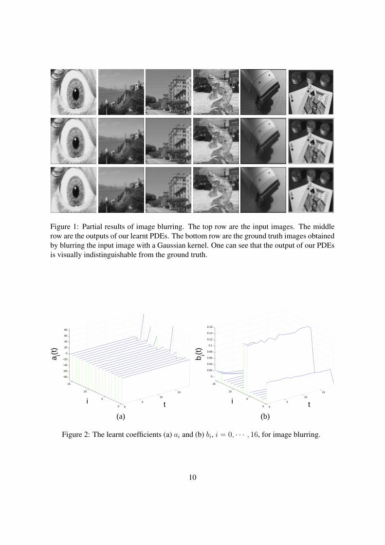
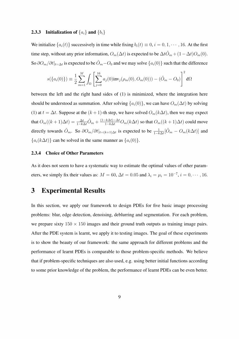
Figure 1: Partial results of image blurring. The top row are the input images. The middlerow are the outputs of our learnt PDEs. The bottom row are the ground truth images obtainedby blurring the input image with a Gaussian kernel. One can see that the output of our PDEsis visually indistinguishable from the ground truth.

0

5

10

15

0

5

10

15

−80

−60

−40

−20

0

20

40

60

80

ti

a i(t)

0

5

10

15

0

5

10

15

0

0.02

0.04

0.06

0.08

0.1

0.12

0.14

0.16

ti

b i(t)

(a) (b)

Figure 2: The learnt coefficients (a) ai and (b) bi, i = 0, ⋅ ⋅ ⋅ , 16, for image blurring.

10

Blurring. For image blurring (Figure 1), the output image is expected to be the convolution

of the input image with a 5 × 5 Gaussian kernel with ¾ = 1. It is well known [11] that this

corresponds to evolving with the standard heat equation Ot = ´(Oxx + Oyy). One can see

from Figure 1 that our learnt PDEs produce outputs that are visually indistinguishable from

the ground truth. Actually, the average per pixel error, measured in root mean squared error,

on the testing images is only 0.46 graylevels. To see whether the learnt PDEs are close to

the ground truth PDEs, we plot the curves of the learnt coefficients in Figure 2. One can

see that the learnt PDEs are not close to the standard heat equation, which corresponds to

a7 = const > 0, ai ≡ 0, i ∕= 7, and bj ≡ 0, j = 0, ⋅ ⋅ ⋅ , 16. This trivial experiment shows

that:

1. the learnt PDEs may be different from the true PDEs that an information process obeys;

2. the learnt PDEs could be effective to produce the expected results at time t = 1;

3. therefore it is unnecessary to retrieve the true PDEs that an information process really

obeys (which may be extremely hard) in order to obtain the desired outputs2.

These observations justify the usefulness of learning-based PDEs.

Edge Detection. For image edge detection (Figure 3), the well-known Canny detector [6]

usually outputs an edge map that includes all edge pixels that are relatively strong within a

certain neighborhood. Hence the resulting edge maps often contain minute edges that may

be visually insignificant. We hope that we can obtain PDEs that output visually salient edges

only. To this end, we select 2 or 3 images from each category of Corel photo library CDs,

where 1 or 2 of them are collected for training and the remaining 1 or 2 images are for

testing. The preparation of the visually salient edge maps is assisted by the edge detector in

[3]3. We first use it to generate relatively rich edge maps and then manually delete visually2In theory, for different mappings there must be inputs such that the outputs of the mappings are different.

However, as natural images are highly structured, they only account for a tiny portion of the Euclidean spacewhose dimension is the number of pixels in the images. So it is possible that different mappings are more orless identical on such a tiny subset of the whole space.

3Code available at http://www4.comp.polyu.edu.hk/∼cslzhang/

11

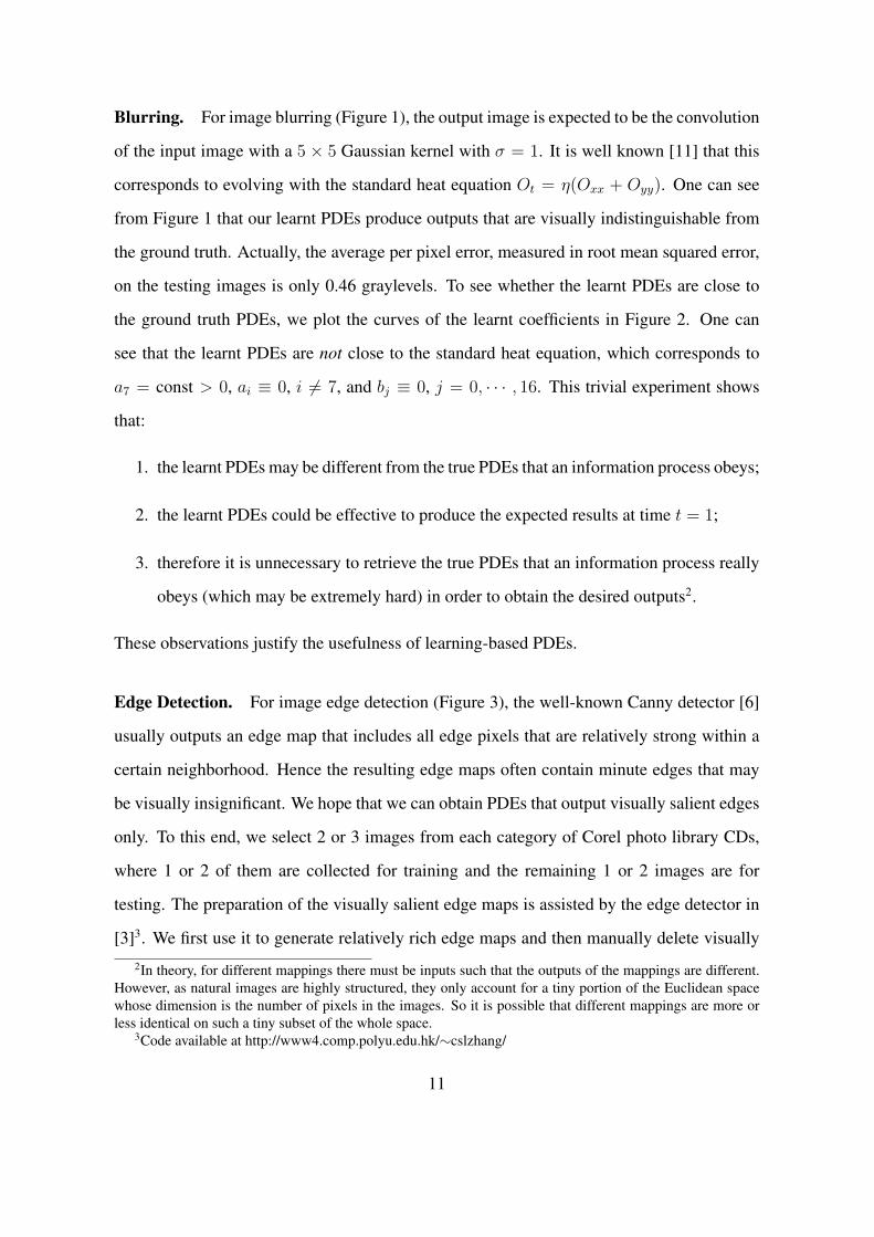
Figure 3: Partial results of edge detection. The top row are the input images. The middlerow are the outputs of our learnt PDEs. The bottom row are the edge maps by the Cannydetector [6].

insignificant edges. In this way, we obtain 60 training image pairs. Figure 3 shows part of

the results on the collected 60 testing images. One can see that our PDEs respond selectively

to edges and basically produce visually significant edges, while the edge maps of the Canny

detector (using the function in Matlab) are more chaotic. Note that the solution of our PDEs

is supposed to be more or less smooth functions. So one cannot expect that our PDEs produce

exactly binary edge maps. Rather, an approximation of binary edge maps is produced.

The curves of the learnt coefficients are shown in Figure 4. Currently we are unable to

analyze the obtained PDEs in detail as this work seems to be non-trivial. So we leave the

analysis to future work.

Denoising. For image denoising (Figure 5), we generate input images by adding zero-mean

Gaussian white noise, with ¾ = 25, to the original noiseless images and use the original

images as the ground truth. One can see from Figure 5 that our PDEs suppress most of the

noise while preserving the edges well. On the testing images, the PSNRs of our PDEs are in

12

0

5

10

15

0

5

10

15

−300

−250

−200

−150

−100

−50

0

50

100

150

ti

a i(t)

0

5

10

15

0

5

10

15

−0.02

−0.015

−0.01

−0.005

0

ti

b i(t)

(a) (b)

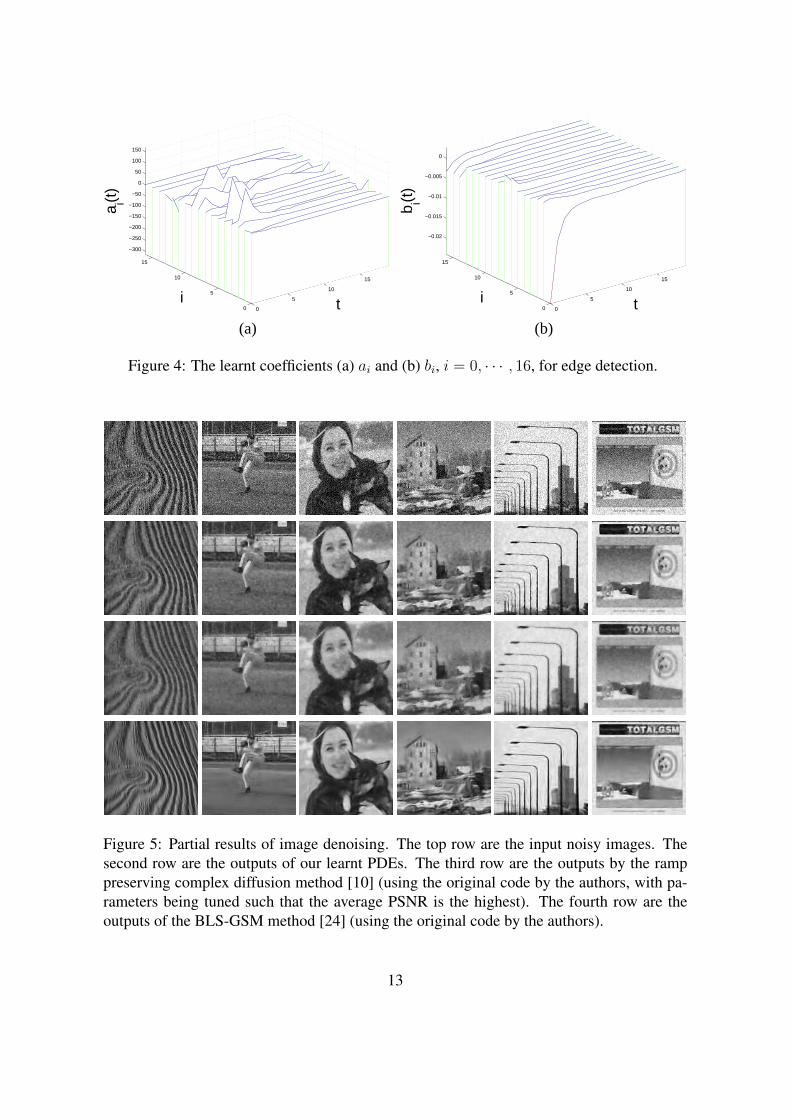
Figure 4: The learnt coefficients (a) ai and (b) bi, i = 0, ⋅ ⋅ ⋅ , 16, for edge detection.

Figure 5: Partial results of image denoising. The top row are the input noisy images. Thesecond row are the outputs of our learnt PDEs. The third row are the outputs by the ramppreserving complex diffusion method [10] (using the original code by the authors, with pa-rameters being tuned such that the average PSNR is the highest). The fourth row are theoutputs of the BLS-GSM method [24] (using the original code by the authors).

13

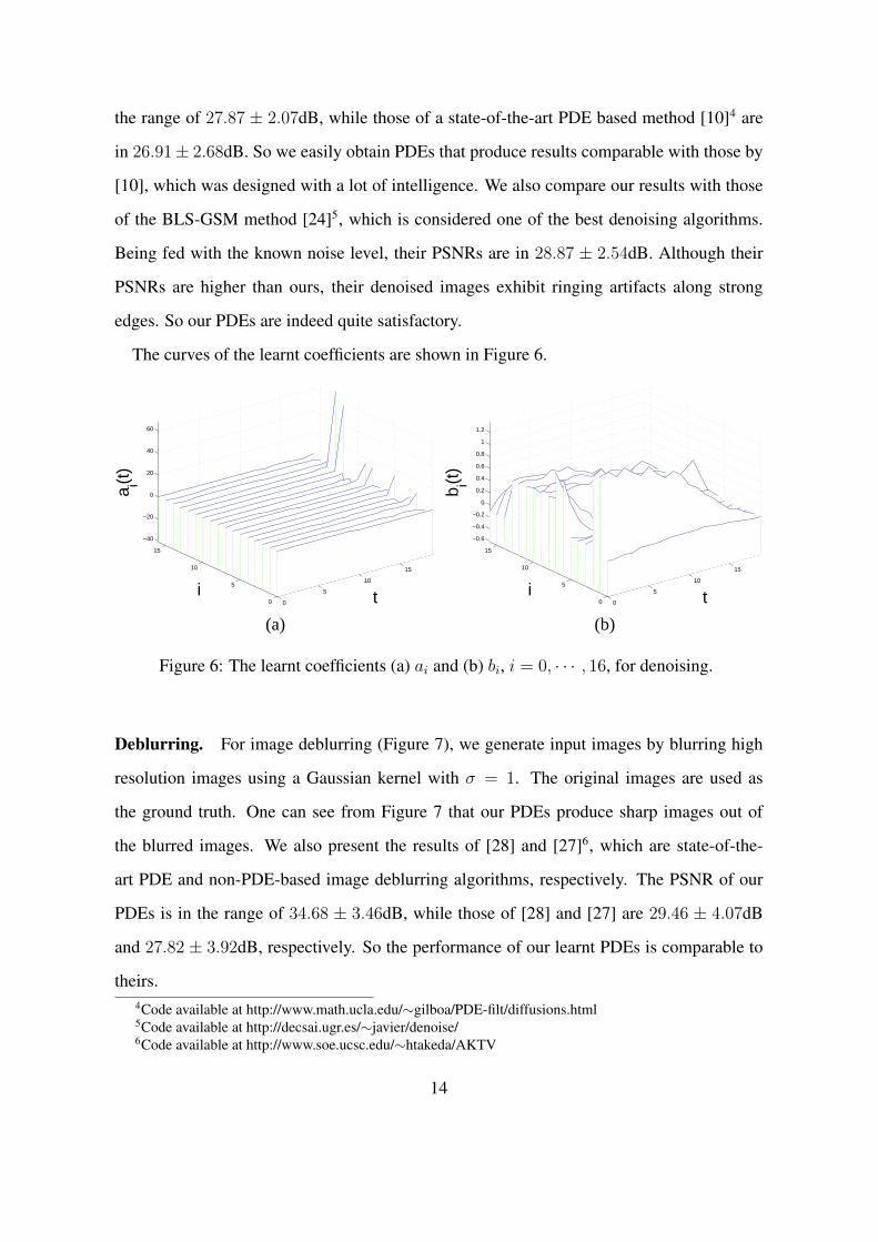
the range of 27.87 ± 2.07dB, while those of a state-of-the-art PDE based method [10]4 are

in 26.91± 2.68dB. So we easily obtain PDEs that produce results comparable with those by

[10], which was designed with a lot of intelligence. We also compare our results with those

of the BLS-GSM method [24]5, which is considered one of the best denoising algorithms.

Being fed with the known noise level, their PSNRs are in 28.87 ± 2.54dB. Although their

PSNRs are higher than ours, their denoised images exhibit ringing artifacts along strong

edges. So our PDEs are indeed quite satisfactory.

The curves of the learnt coefficients are shown in Figure 6.

0

5

10

15

0

5

10

15

−40

−20

0

20

40

60

ti

a i(t)

0

5

10

15

0

5

10

15

−0.6

−0.4

−0.2

0

0.2

0.4

0.6

0.8

1

1.2

ti

b i(t)

(a) (b)

Figure 6: The learnt coefficients (a) ai and (b) bi, i = 0, ⋅ ⋅ ⋅ , 16, for denoising.

Deblurring. For image deblurring (Figure 7), we generate input images by blurring high

resolution images using a Gaussian kernel with ¾ = 1. The original images are used as

the ground truth. One can see from Figure 7 that our PDEs produce sharp images out of

the blurred images. We also present the results of [28] and [27]6, which are state-of-the-

art PDE and non-PDE-based image deblurring algorithms, respectively. The PSNR of our

PDEs is in the range of 34.68 ± 3.46dB, while those of [28] and [27] are 29.46 ± 4.07dB

and 27.82 ± 3.92dB, respectively. So the performance of our learnt PDEs is comparable to

theirs.4Code available at http://www.math.ucla.edu/∼gilboa/PDE-filt/diffusions.html5Code available at http://decsai.ugr.es/∼javier/denoise/6Code available at http://www.soe.ucsc.edu/∼htakeda/AKTV

14

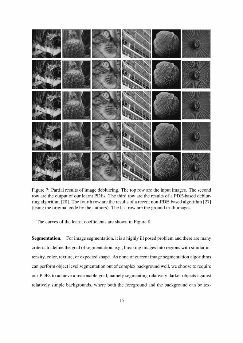
Figure 7: Partial results of image deblurring. The top row are the input images. The secondrow are the output of our learnt PDEs. The third row are the results of a PDE-based deblur-ring algorithm [28]. The fourth row are the results of a recent non-PDE-based algorithm [27](using the original code by the authors). The last row are the ground truth images.

The curves of the learnt coefficients are shown in Figure 8.

Segmentation. For image segmentation, it is a highly ill posed problem and there are many

criteria to define the goal of segmentation, e.g., breaking images into regions with similar in-

tensity, color, texture, or expected shape. As none of current image segmentation algorithms

can perform object level segmentation out of complex background well, we choose to require

our PDEs to achieve a reasonable goal, namely segmenting relatively darker objects against

relatively simple backgrounds, where both the foreground and the background can be tex-

15

0

5

10

15

0

5

10

15

−200

−150

−100

−50

0

50

100

ti

a i(t)

0

5

10

15

0

5

10

15

−0.4

−0.2

0

0.2

0.4

0.6

tib i(t

)(a) (b)

Figure 8: The learnt coefficients (a) ai and (b) bi, i = 0, ⋅ ⋅ ⋅ , 16, for deblurring.

Figure 9: Examples of the training images for image segmentation. In each group of images,on the left is the input image and on the right is the ground truth output mask.

16

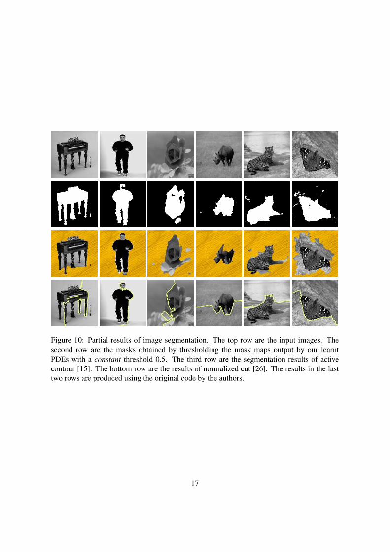
Figure 10: Partial results of image segmentation. The top row are the input images. Thesecond row are the masks obtained by thresholding the mask maps output by our learntPDEs with a constant threshold 0.5. The third row are the segmentation results of activecontour [15]. The bottom row are the results of normalized cut [26]. The results in the lasttwo rows are produced using the original code by the authors.

17

tured and simple thresholding cannot separate them. So we select 60 images with relatively

darker foregrounds and relatively simple backgrounds, but the foreground is not of uniformly

lower graylevels than the background, and prepare the manually segmented binary masks as

the outputs of the training images (Figure 9). Part of the segmentation results are shown in

Figure 10, where we have thresholded the output mask maps of our learnt PDEs with a con-

stant threshold 0.5. We see that our learnt PDEs produce fairly good object masks. We also

test the active contour method by Li et al. [15]7 and the celebrated normalized cut method

[26]8. One can see from Figure 10 that the active contour method [15] cannot segment object

details due to its smoothness constraint on the object shape and the normalized cut method

[26] cannot produce a closed foreground region. To provide quantitative evaluation, we use

the F -measure that merges the precision and recall of segmentation:

F® =(1 + ®) ⋅ recall ⋅ precision® ⋅ precision+ recall

, where

recall =∣A ∩B∣∣A∣ , precision =

∣A ∩B∣∣B∣ ,

in which A is the ground truth mask, B is the computed mask and ∣ ⋅ ∣ denotes the area of a

region. The most common choice of ® is 2. On our testing images, the F2 measures of our

PDEs, [15] and [26] are 0.90± 0.05, 0.83± 0.16 and 0.61± 0.20, respectively. One can see

that the performance of our PDEs is better than theirs, in both visual quality and quantitative

measure.

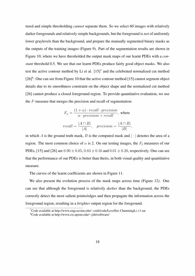
The curves of the learnt coefficients are shown in Figure 11.

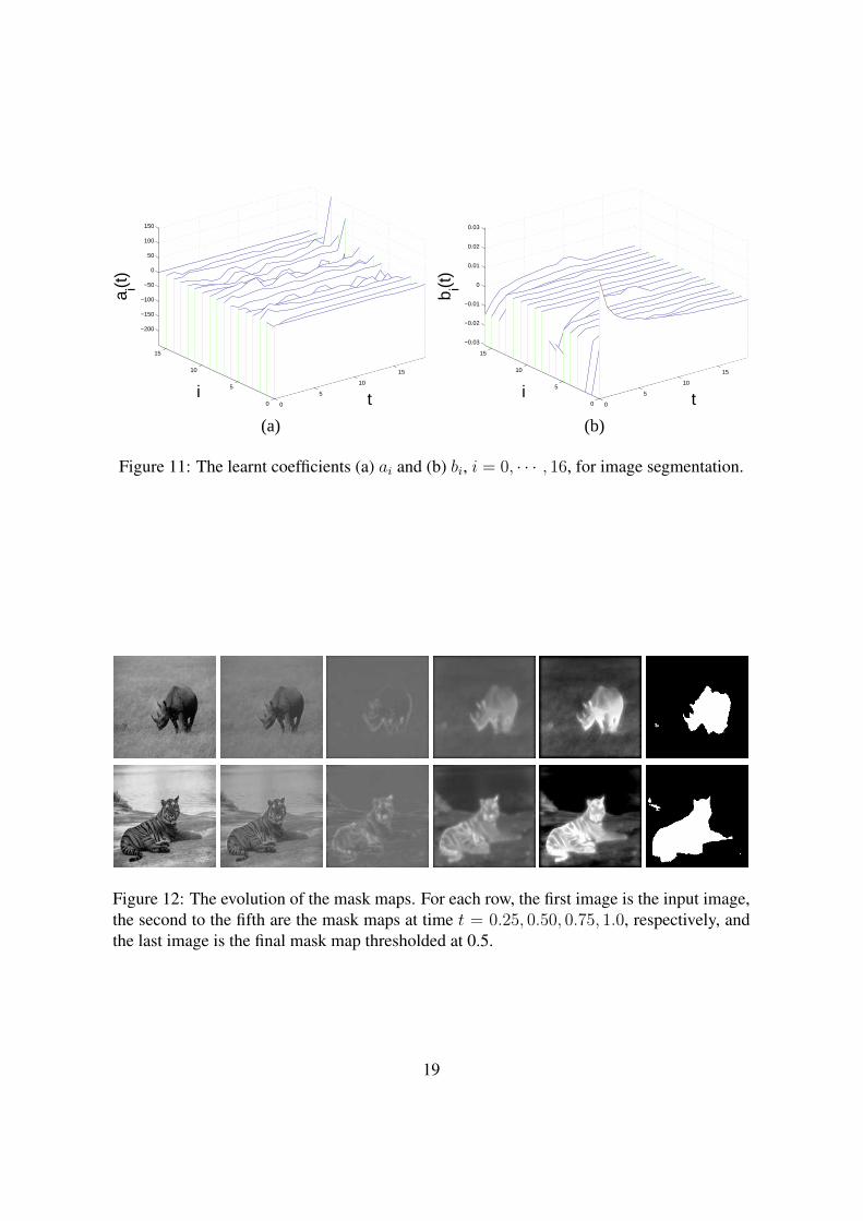
We also present the evolution process of the mask maps across time (Figure 12). One

can see that although the foreground is relatively darker than the background, the PDEs

correctly detect the most salient points/edges and then propagate the information across the

foreground region, resulting in a brighter output region for the foreground.

7Code available at http://www.engr.uconn.edu/∼cmli/code/LevelSet ChunmingLi v1.rar8Code available at http://www.cis.upenn.edu/∼jshi/software/

18

0

5

10

15

0

5

10

15

−200

−150

−100

−50

0

50

100

150

ti

a i(t)

0

5

10

15

0

5

10

15

−0.03

−0.02

−0.01

0

0.01

0.02

0.03

ti

b i(t)

(a) (b)

Figure 11: The learnt coefficients (a) ai and (b) bi, i = 0, ⋅ ⋅ ⋅ , 16, for image segmentation.

Figure 12: The evolution of the mask maps. For each row, the first image is the input image,the second to the fifth are the mask maps at time t = 0.25, 0.50, 0.75, 1.0, respectively, andthe last image is the final mask map thresholded at 0.5.

19

4 Conclusions and Future Work

In this paper, we have presented a framework of learning PDEs from examples for image

processing problems. The experimental results on some image processing problems show

that our theory is promising. However, the current work is still preliminary; we plan to push

our research in the following directions.

First, we will apply our framework to more image processing/computer vision problems

to find out to what extent it works. We do find some problems, e.g., image inpainting, that

our current framework does not work well. But we also want to find more problems that

our current framework works well. This would help us understand the level of complexity

of image processing/computer vision problems. Second, the time required to learn the PDEs

is a bit long. On our 2.4GHz Duro Core Pentium PC, the time is about 3 days, using our

unoptimized codes. Note that such a time frame may still be shorter than that for a human

to design PDEs as effective for the same problem. Although the computation can easily

be parallelized, better mechanisms, e.g., better initialization of the combination coefficients

and real-time optimal control techniques [5], should be explored. Third, although hard,

the theoretical analysis on our approach, e.g., the well-posedness of the learnt PDEs and

the numerical stability condition for the temporal stepsize Δt, should be tried. Fourth, it is

attractive to analyze the learnt PDEs and find out their connections with the biological vision;

we hope to borrow some ideas from the biological vision. We expect that someday learning-

based PDEs, in their improved formulations, could be a general framework for designing

PDEs for most image processing problems.

References

[1] Alvarez, L., Guichard, F., Lions, P.L., Morel, J.M.: Axioms and fundamental equations

of image processing. Arch. for Rational Mechanics 123(3), 199–257 (1993)

[2] Aubert, G., Kornprobst, P.: Mathematical Problems in Image Processing. Springer-

Verlag (2002)

20

[3] Bao, P., Zhang, L., Wu, X.: Canny edge detection enhancement by scale multiplication.

IEEE Trans. Pattern Analysis and Machine Intelligence 27(9), 1485–1490 (2005)

[4] Bertalmio, M., Sapiro, G., Caselles, V., Ballester, C.: Image inpainting. In: SIG-

GRAPH, pp. 417–424 (2000)

[5] Biegler, L., et al.: Real-Time PDE-Constrained Optimization. SIAM (2007)

[6] Canny, J.: A computational approach to edge detection. IEEE Trans. Pattern Analysis

and Machine Intelligence 8, 679–714 (1986)

[7] Cao, F.: Geometric Curve Evolution and Image Processing. Lecture Notes in Mathe-

matics, No. 1805. Springer-Verlarg (2003)

[8] Caselles, V., Morel, J.M., Sapiro, G., A. Tannenbaum (eds.): Special issue on partial

differential equations and geometry-driven diffusion in image processing and analysis.

IEEE Trans. Image Processing 7(3) (1998)

[9] Gabor, D.: Information theory in electron microscopy. Laboratory Investigation 14,

801–807 (1965)

[10] Gilboa, G., Sochen, N., Zeevi, Y.: Image enhancement and denoising by complex dif-

fusion processes. IEEE Trans. Pattern Analysis and Machine Intelligence 26(8), 1020–

1036 (2004)

[11] ter Haar Romeny, B.M.: Geometry-Driven Diffusion in Computer Vision. Kluwer

Academic Publishers (1994)

[12] Jain, A.: Partial differential equations and finite-difference methods in image process-

ing, part 1. J. Optimization Theory and Applications 23, 65–91 (1977)

[13] Kimia, B., Tannenbaum, A., Zucker, S.: On optimal control methods in computer vision

and image processing. In B. ter Haar Romeny (ed.) Geometry-Driven Diffusion in

Computer Vision, Kluwer Academic Publishers, 1994

21

[14] Koenderink, J.: The structure of images. Biological Cybernetics 50, 363–370 (1984)

[15] Li, C., Xu, C., Gui, C., Fox, M.: Level set evolution without re-initialization: A new

variational formulation. In: Proc. Computer Vision and Pattern Recognition (2005)

[16] Lin, Z., Zhang, W., Tang, X.: Learning partial differential equations for computer vi-

sion (2008). Microsoft Technical Report #MSR-TR-2008-189

[17] Lions, J.L.: Optimal Control Systems Governed by Partial Differential Equations.

Springer-Verlarg (1971)

[18] Mikolajczyk, K., Schmid, C.: A performance evaluation of local descriptors. IEEE

Trans. Pattern Analysis and Machine Intelligence 27(10), 1615–1630 (2005)

[19] Olver, P.: Applications of Lie Groups to Differential Equations. Springer-Verlarg, New

York (1993)

[20] Osher, S., Rudin, L.I.: Feature-oriented image enhancement using shock filters. SIAM

J. Numerical Analysis 27(4), 919–940 (1990)

[21] Papadakis, N., Corpetti, T., Memin, E.: Dynamically consistent optical flow estimation.

In: Proc. Intn’l Conf. Computer Vision (2007)

[22] Papadakis, N., Memin, E.: Variational optimal control technique for the tracking of

deformable objects. In: Proc. Int. Conf. Computer Vision (2007)

[23] Perona, P., Malik, J.: Scale-space and edge detection using anisotropic diffusion. IEEE

Trans. Pattern Analysis and Machine Intelligence 12(7), 629–639 (1990)

[24] Portilla, J., Strela, V., Wainwright, M., Simoncelli, E.: Image denoising using scale

mixtures of Gaussians in the wavelet domain. IEEE Trans. mage Processing 12(11),

1338–1351 (2003)

[25] Sapiro, G.: Geometric Partial Differential Equations and Image Analysis. Cambridge

University Press (2001)

22

[26] Shi, J., Malik, J.: Normalized cuts and image segmentation. IEEE Trans. Pattern Anal-

ysis and Machine Intelligence 22(8), 888–905 (2000)

[27] Takeda, H., Farsiu, S., Milanfar, P.: Deblurring using regularized locally adaptive ker-

nel regression. IEEE Trans. Image Processing 17(4), 550–563 (2008)

[28] Welk, M., Theis, D., Brox, T., Weickert, J.: PDE-based deconvolution with forward-

backward diffusivities and diffusion tensors. In: Proc. Scale Space and PDE Methods

in Computer Vision, pp. 585–597 (2005)

[29] Witkin, A.: Scale-space filtering. In: Proc. Int. Joint Conf. Artificial Intelligence (1983)

Appendix 1: Shift Invariance of PDEs

We prove that the coefficients aj and bj must be independent of x.

Proof: We prove for LO only. We may rewrite

LO(a(x, t), ⟨O⟩, ⟨½⟩) = LO(⟨O⟩, ⟨½⟩,x, t),

and it suffices to prove that LO is independent of x.

By the definition of shift invariance, when I(x) changes to I(x − x0) by shifting with a

displacement x0, O(x) and ½(x) will change to O(x − x0) and ½(x − x0), respectively. So

the pair (½(x− x0), O(x− x0)) fulfils (1), i.e.,

∂O(x− x0)

∂t= LO(⟨O(x− x0)⟩, ⟨½(x− x0)⟩,x, t)= LO(⟨O⟩(x− x0), ⟨½⟩(x− x0),x, t).

(5)

Next, we replace x− x0 in the above equation with x and have:

∂O(x)

∂t= LO(⟨O⟩(x), ⟨½⟩(x),x+ x0, t). (6)

On the other hand, the pair (½(x), O(x)) also fulfils (1), i.e.,

∂O(x)

∂t= LO(⟨O⟩(x), ⟨½⟩(x),x, t). (7)

23

Therefore,

LO(⟨O⟩(x), ⟨½⟩(x),x+ x0, t) = LO(⟨O⟩(x), ⟨½⟩(x),x, t),

∀x0 that confines the input image inside Ω.

So LO is independent of x.

□

Appendix 2: The Gateaux Derivatives

We compute the Gateaux derivatives by perturbation. The underlying theory can be found in

[16, 21, 22]. The Lagrangian function is:

J({Om}Mm=1, {aj}16j=0, {bj}16j=0; {'m}Mm=1, {Ám}Mm=1)= J({Om}Mm=1, {aj}16j=0, {bj}16j=0)

+M∑

m=1

∫

Q

'm [(Om)t − LO(a, ⟨Om⟩, ⟨½m⟩)] dQ

+M∑

m=1

∫

Q

Ám [(½m)t − L½(b, ⟨½m⟩, ⟨Om⟩)] dQ,

(8)

where 'm and Ám are the adjoint functions.

To find the adjoint equations for 'm, we perturb LO and L½ with respect to O. The

perturbations can be written as follows:

LO(a, ⟨O + " ⋅ ±O⟩, ⟨½⟩)− LO(a, ⟨O⟩, ⟨½⟩)= " ⋅

(∂LO

∂O(±O) +

∂LO

∂Ox

∂(±O)

∂x+ ⋅ ⋅ ⋅+ ∂LO

∂Oyy

∂2(±O)

∂y2

)+ o(")

= "∑p∈℘

∂LO

∂Op

∂∣p∣(±O)

∂p+ o(")

= "∑p∈℘

¾O;p∂∣p∣(±O)

∂p+ o("),

L½(b, ⟨½⟩, ⟨O + " ⋅ ±O⟩)− L½(b, ⟨½⟩, ⟨O⟩)= "

∑p∈℘

¾½;p∂∣p∣(±O)

∂p+ o("),

(9)

24

where

℘ = {∅, x, y, xx, xy, yy},∣p∣ = the length of string p,

¾O;p =∂LO

∂Op

=16∑i=0

ai∂invi(½,O)

∂Op

, and

¾½;p =∂L½

∂Op

=16∑i=0

bi∂invi(O, ½)

∂Op

.

Then the difference in J caused by perturbing Ok only is

±Jk= J(⋅ ⋅ ⋅ , Ok + " ⋅ ±Ok, ⋅ ⋅ ⋅ )− J(⋅ ⋅ ⋅ , Ok, ⋅ ⋅ ⋅ )=

1

2

∫

Ω

[((Ok + " ⋅ ±Ok)(x, 1)− Ok(x)

)2

−(Ok(x, 1)− Ok(x)

)2]

dΩ

+

∫

Q

'k {[(Ok + " ⋅ ±Ok)t − LO(a, ⟨Ok + " ⋅ ±Ok⟩, ⟨½k⟩)]− [(Ok)t − LO(a, ⟨Ok⟩, ⟨½k⟩)]} dQ

+

∫

Q

Ák {[(½k)t − L½(b, ⟨½k⟩, ⟨Ok + " ⋅ ±Ok⟩)] − [(½k)t − L½(b, ⟨½k⟩, ⟨Ok⟩)]} dQ

= "

∫

Ω

(Ok(x, 1)− Ok(x)

)±Ok(x, 1)dΩ + "

∫

Q

'k(±Ok)tdQ

−"

∫

Q

'k

∑p∈℘

¾O;p∂∣p∣(±Ok)

∂pdQ− "

∫

Q

Ák

∑p∈℘

¾½;p∂∣p∣(±Ok)

∂pdQ+ o(").

(10)

As the perturbation ±Ok should satisfy that

±Ok∣Γ = 0 and ±Ok∣t=0 = 0,

due to the boundary and initial conditions of Ok, if we assume that

'k∣Γ = 0,

25

then integrating by parts, the integration on the boundary Γ will vanish. So we have

±Jk

= "

∫

Ω

(Ok(x, 1)− Ok(x)

)±Ok(x, 1)dΩ

+"

∫

Ω

('k ⋅ ±Ok)(x, 1)dΩ− "

∫

Q

('k)t±OkdQ

−"

∫

Q

∑p∈℘

(−1)∣p∣∂∣p∣(¾O;p'k)

∂p±OkdQ

−"

∫

Q

∑p∈℘

(−1)∣p∣∂∣p∣(¾½;pÁk)

∂p±OkdQ+ o(")

= "

∫

Q

[('k +Ok(x, 1)− Ok(x)

)±(t− 1)

− ('k)t − (−1)∣p∣∂∣p∣(¾O;p'k + ¾½;pÁk)

∂p

]±OkdQ+ o(").

(11)

By letting " → 0, we have that the adjoint equation for 'k is⎧⎨⎩

∂'m

∂t+∑p∈℘

(−1)∣p∣ (¾O;p'm + ¾½;pÁm)p = 0, (x, t) ∈ Q,

'm = 0, (x, t) ∈ Γ,

'm∣t=1 = Om −Om(1), x ∈ Ω,

(12)

in order that ∂J∂Ok

= 0. Similarly, the adjoint equation for Ák is⎧⎨⎩

∂Ám

∂t+∑p∈℘

(−1)∣p∣ (¾O;p'm + ¾½;pÁm)p = 0, (x, t) ∈ Q,

Ám = 0, (x, t) ∈ Γ,Ám∣t=1 = 0, x ∈ Ω,

(13)

where

¾O;p =∂LO

∂½p=

16∑i=0

ai∂invi(½,O)

∂½p, and

¾½;p =∂L½

∂½p=

16∑i=0

bi∂invi(O, ½)

∂½p.

(14)

Also by perturbation, it is easy to check that:

∂J

∂ai= ¸iai −

∫

Ω

M∑m=1

'minvi(½m, Om)dΩ,

∂J

∂bi= ¹ibi −

∫

Ω

M∑m=1

Áminvi(Om, ½m)dΩ.

The above are also the Gateaux derivatives of J with respect to ai and bi, respectively.

26