Design of a Cure Monitoring System for Composite Aircraft Repair Patches

Dean DeVries

A thesis submitted in conforrnity with the requirements for the degree of Master of Applied Science

Graduate Department of Aerospace Engineering University of Toronto

S Copyright by Dean DeVrîes, 1996

National Library 1+1 .,nad Bibliothèque nationale du Canada

Acquisitions and Acquisitions et Bibliogtaphic Services seivices bibliographiques

395 Wellington Street 395, ruet Wellington Onawa ON K1A ON4 ûttawa ON K1 A ON4 Canada Canada

The author has granted a non- exclusive licence aüowing the National Library of Canada to reproduce, loan, distribute or seil copies of this thesis in microform, paper or elecîronic formats.

The author retains ownership of the copyright in this thesis. Neither the thesis nor substantial extracts fiom it may be printed or otherwise reproduced without the author's permission.

L'auteur a accordé une licence non exclusive permettant a la Bibliothèque nationale du Canada de reproduire, prêter, distribuer ou vendre des copies de cette thèse sous la forme de microfiche/6im, de reproduction sur papier ou sur format électronique.

L'auteur conserve la propriété du droit d'auteur qui protège cette thèse. Ni la thèse ni des extraits substantiels de celle-ci ne doivent être imprimés ou autrement reproduits sans son autorisation.

Abstract

Aircr& repair patches make use of thermosetting polymers and the quality of the repair depends on proper curing. The design of a cure monitoring system for aircraft repair patches is explored. Cure monitoring was achieved by measuring the signal strength and tirne of flight of an ultrasonic wave transmitted through the material. Custom traasducers, electronics and software was designed for the system.

Preliminary resuits were encouraging. The present system does not provide accurate measurements of time of flight and thus cm not provide a quantitative assessrnent of the material properties. However, qualitative results based on changes in signai strength provided important information regarding the state of cure of the thermoset. Several cure tests accompanied by mechanical tests demonstrated the usefulness of the present system. Recornmendations for creating a commercially viable system are given.

The system was used to evaluate the practicality of Bragg grathg fibre optic sensors as cure monitoring devices. Bragg gratings do not appear to produce useful cure related data.

Acknowledgements

The author would like to recognize the contributions of the foliowing:

Prof. R.C. T ~ M Y S O ~ , Dr. W.D. M O ~ S O ~ and Gerald Manuelpiilai o f the Aerospace Materials Group at UTIAS for their excellent advice and invaluable assistauce.

Dr. Sharon Huang and Dr. Michel LeBlanc from the Fibre Optics Smart Structures lab at UTIAS for their assistance with the Bragg grating experirnents.

Dr. Stuart Foster, Leo Zan and Brian Starkowski from the Ultrasonics group at Sunnybrook Health Sciences Centre for their considerable help.

The Ontario Centre for Materials Research for their generous fmancial support.

Table of Contents

. . . . . . . . . . . . . . . . . . . . . . . . . . . . . . . . . . . . . . . . . . . . . . . . . . . . . . Nomenclature v

2 . Cure and Cure Monitoring . . . . . . . . . . . . . . . . . . . . . . . . . . . . . . . . . . . . . . . . . . . 3 . . . . . . . . . . . . . . . . . . . . . . . . . . . . . . . . . . . . . . 2.1 The curing of thennosets 3

2.2 Methods for cure monitoring . . . . . . . . . . . . . . . . . . . . . . . . . . . . . . . . . . . 4

. . . . . . . . . . . . . . . . . . . . . . . . . . . . . . . . . . . . . . . . . . 3 . Ultrasonic Cure Monitoring 6 . . . . . . . . . . . . . . . . . . . . . . . . . . . . . . . . 3.1 Acoustic wave in elastic medium 6

. . . . . . . . . . . . . . . . . . . . . . . . . . . . . . . . . . . . . 3.2 Acoustic wave in a fluid I l . . . . . . . . . . . . . . . . . . . . . . . . . . . . . . . . . . . . 3.3 The Ultrasonic Transducer 12

. . . . . . . . . . . . . . . . . . . . . . . . . . . . . . . . . 3.3.1 Piezoelectric Material 12 . . . . . . . . . . . . . . . . . . . . . . . 3.3.2 Broad-band Traasducer Construction 15

. . . . . . . . . . . . . . . . . . . . . . . . . . . 3.4 CMS Transducer Design Considerations 17

. . . . . . . . . . . . . . . . . . . . . . . . . . . . . . . . . . 4 . The UTIAS Cure Monitoring System 19 . . . . . . . . . . . . . . . . . . . . . . . . . . . . . . . . . . . . . . . . . . . . . 4.1. Transducers 19

. . . . . . . . . . . . . . . . . . . . . . . . . . . . . . . . . . . . . . . . . . . . . . 4.2 Electronics 21 . . . . . . . . . . . . . . . . . . . . . . . . . . . . . . . . . . . . 4.3 Cure Monitoring Software 23

. . . . . . . . . . . . . . . . . . . . . . . . . . . . . . . . . . . . . . . . . . . . . . . 5 . CMS Performance 23 . . . . . . . . . . . . . . . . . . . . . . . . . . . . . . . . . . . . 5.1 Temperature Dependence 24

. . . . . . . . . . . . . . . . . . . . . . . . . . . . . . . . . . 5.2 CMS Electronics Performance 25 . . . . . . . . . . . . . . . . . . . 5.3 Qualitative Cure Monitoring Using Signal Strength 26

5.4 Evaluation of the use of Bragg Grating fibre optic . . . . . . . . . . . . . . . . . . . . . . . . . . . . . . . . . . sensors for cure monitoring 39

. . . . . . . . . . . . . . . . . . . . . . . . . . . . . . . . . . . . . . . . . . . . . . . . . . . 6 . Conclusions 31

. . . . . . . . . . . . . . . . . . . . . . . . . . . . . . . . . . . . . . . . . . . . . . . . . . . . . 7 . References 32

Table 1 Effect of Attenuation on Wave Speed . . . . . . . . . . . . . . . . . . . . . . . . . . . . . . . 9 Table 2 Cornparison of Piezoelectnc Materials . . . . . . . . . . . . . . . . . . . . . . . . . . . . . . 14

............................................ Table 3 Sample Properties 28

Nomenclature

visco-elastic attenuation of ultrasonic wave in direction i (m*') initial amplitude on an ultrasonic wave wave speed in direction i ( d s ) wave speed of a wave in an ideal elastic solid c=FYlp indices. i j,k,l = 1 ..3 electro-mechanical coupling factors for a piezoelectric element wave propagation constant K, = &/ci generai material stifiess, F = F' + iF" component of material stifkess tensor. Qiju = Qijki + fQbu mechanical quality factor for a thin disc of piezoelectric material tirne cure temperature Curie temperature glas transition temperature component of displacement component of location vector characteristic acoustic impedance of a mateid. Z=pc

direction cosines of particle displacement vector direction cosines of wave propagation vector reflection and transmission coefficients of an ultrasonic wave crossing a material interface p/p delta function 4, = 1 if i=k and zero otherwise permittivity of fiee space E,, = 8.8542~ 1 O*'* F/m component of strain tensor material density component of stress tensor radial fiequency of ultrasonic wave

Tensor

d piezoelectric constant. d=(D,,), = (e,& D electric displacement flux density e piezoelectnc constant. r@,3, = -(@,de E electric field g piezoelectnc constant. g==e,& = -(EJD h piezoelectric constant. h=-(EJD = -(u,,), K wave propagation constant vector P dipole moment pet unit volume

material stiffiiess material cornpliance

particle displacement vector wave propagation vector dielectric permittivity str ain stress dielectric impermeabiiity

Conventions

9.a

a.. . I J J

OE OT O* det A

ahi - t afler at2 aus - indice

ax,

comma indicates time derivative

after comma indicates spatial denvative

operation in () at constant E transpose of tensor complex conjugate determinant of A

Acron yms

BFOS CMS CSSA EM FRP GRE NDE TOF PZT UTIAS

Bragg Grating Fibre Optic Sensor Cure Monitoring System Constant Signal Strength Amplifier Electro-Magnetic Fibre Reinforced Polymer Graphite Reinforced Epoxy Non-Destructive Evaluation Time Of Flight Lead (Pb) Zirconate Titanate University of Toronto losthte for Aerospace Studies

"... national or internationai standards for repair processes and composite material specifications need to be established. It is clear that airfiame manufacturers and vendors have some catching up to do to ensure that airlines with advanced composites used in daily operations know how to repair them with minimal cost and schedule impact. The headache today for maintenance crews will be the financial problem tomorrow for an airline's fiont office, where increased overhead and repair tirnes eventually reach the bottom line."

Edimrial. "Airframen Should Help Mainfain Composites," Aviation Wcek & S p a Technology. Jan 2, 1995.

1. Introduction

Society has significantly benefitted fiom the development of fibre relliforced polymer

(FRP) composites. Such diverse applications as automobile bodies, canoes and golf clubs

make us of these materials. In addition to high relative stifhess and strength to weight ratios,

FRPs offer the user the ability to "tailor" the mechanical properties of a structure. A specific

application for FRPs which will be discussed is aircraft repair patches.

A study conducted by the Aeronautical Research Laboratory in Australia [Baker]

examined the use of adhesively bonded composite patches to arrest fatigue/stress-corrosion

induced cracking. The same study lists the following uses for such patches: stiffen

underdesigned regions, restore lost strength or stifniess, reduce stress concentrations and

improve damage tolerance. In addition to the above applications, composite patches could be

used to restore the aerodynamics of a vehicle (by tepairing skin damage) and improve the

damping of structures.

Probably the most popular type of FRP used today are fibre reinforced thennosets - principally those which use epoxy as the mat*. Thermoset ma& materials are less

expensive than thermoplastics, and can be used to form complex shapes. Such materials are

favoured for adhesively bonded repair patches. The characteristic feature of a thermoset is

its need to be cured. These materials are initially a viscous liquid(s) and undergo a chemical

reaction (curing) by which they become solids. Proper cure is vital for achieving the

maximum mechanical properties of the material.

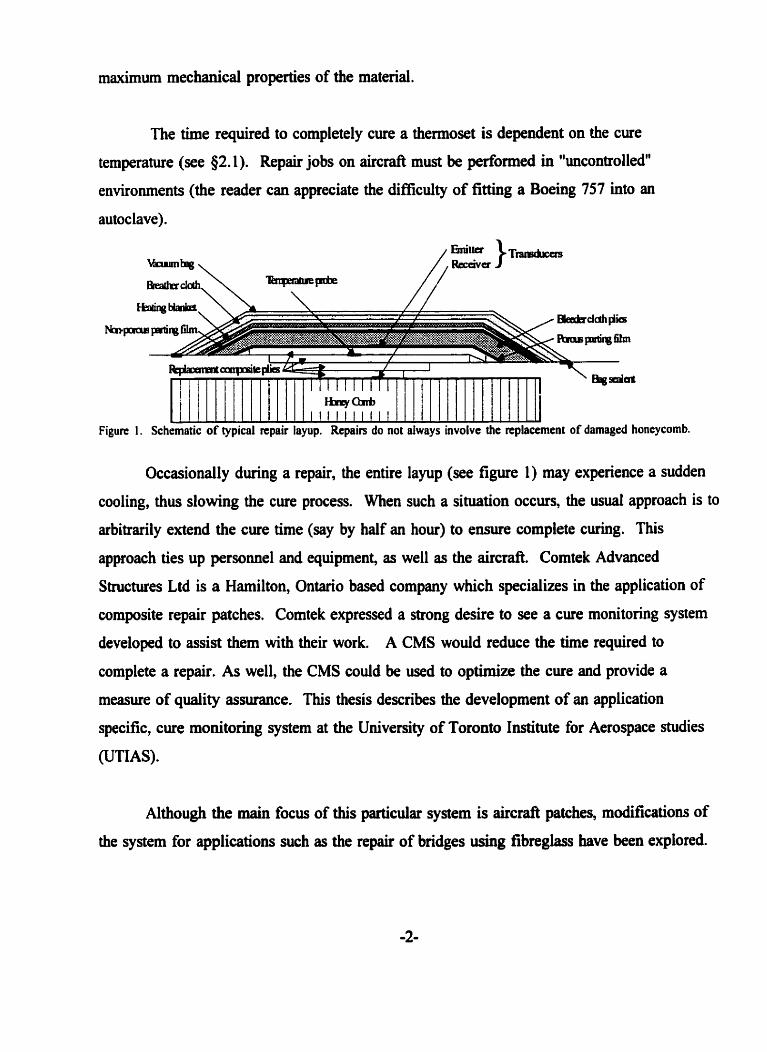
The time requVed to completely cure a thermoset is dependent on the cure

temperature (see 82.1). Repair jobs on aircrafl rnust be performed in "uncontrolled"

environments (the reader can appreciate the difficulty of fitting a Boeing 757 into an

autoclave).

Figure 1. Schematic of typical repair layup. Repairs do not aIways involve the replacement of damagrd honeycomb.

Occasiondly during a repair, the entire layup (see figure 1) may experience a sudden

cooling, thus slowing the cure process. When such a situation occurs, the usuai approach is to

arbitrarily extend the cure time (say by half an hour) to eiisure complete curing. This

approach ties up personnel and equipment, as well as the aircraft. Comtek Advanced

Structures Ltd is a Hamilton, Ontario based Company which specializes in the application of

composite repair patches. Comtek expressed a strong desire to see a cure monitoring system

developed to assist them with their work. A CMS would reduce the time required to

complete a repair. As well, the CMS could be used to optimize the cure and provide a

measure of quality assurance. This thesis describes the development of an application

specific, cure monitoring system at the University of Toronto Institute for Aerospace studies

(UWS).

Although the main focus of this particular system is aircraft patches, modifications of

the system for applications such as the repair of bridges using fibreglass have been explored.

2. Cure and Cure Monitoring

2.1 The curing of thermosets

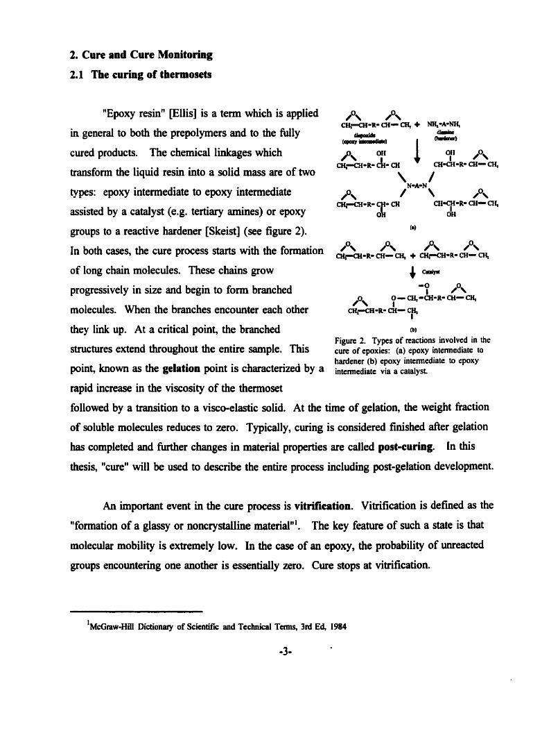
"Epoxy resin" [Ellis] is a term which is applied p, A CEQ--R- CH- Cy + W - A œ m

in general to both the prepolymers and to the Mly - diRliœ

(w -1 I -)

cured products. The chernical linkages which A OH or /O\

w--R- di- CH CEï-CH-R- CH- CH, transfonn the liquid resin into a solid mass are of two \ / types: epoxy intermediate to epoxy intemediate A ; /O\ - - CHICH-R- CH- CH,

assisted by a catalyst (e.g. tertiary amines) or epoxy OH I

groups to a reactive hardener [Skeist] (see figure 2). (8)

/O\ P\ A P\ In both cases, the cure process starts with the formation q-QI-Rœ CH- M, + w-CCI.R- CH- CY

of long chah molecules. These chains grow 4- progressively in size and begin to f o m branched -0 , A

A O - CH, -CH-R- CH- C&

molecules. When the branches encounter each other I CIQICFI-R- CH- CH,

I

they Iink up. At a critical point, the branched (W

Figure 2. Types o f reactions involved in the structures extend throughout the entire sample. This of epoxics: (a) epoxy intemediate to

hardcncr (b) cpoxy intemediate to epony point, known as the gelation point is characterized by a inkmediate , , ,hiyst

rapid increase in the viscosity of the thermoset

followed by a transition to a visco-elastic solid. At the tirne of gelation, the weight fraction

of soluble molecules reduces to zero. Typically, curing is considered fdshed after gelation

has completed and M e r changes in materiai properties are called post-curing. In this

thesis, "cure" will be used to describe the entire process including pst-gelation development.

An important event in the cure process is vitrifhation. Vitrification is defined as the

"formation of a glassy or noncrystalline material"'. The key feature of such a state is that

molecular mobility is extremely low. In the case of an epoxy, the probability of unreacted

groups encountering one another is essentially zero. Cure stops at vitrification.

l ~ ~ ~ m ~ - ~ i l l Dictionary of Scientific and Technical Temg 3rd Ed, 1984

Associated with vitrification is the glass transition temperature (TJ. The value of Tg

increases over the course of the cure. As long as the cure temperature (T3 is much larger

than Tg the reaction rate remains kinetically controlled. However, if the difference between

Tc and Tg is allowed to become srnail, the reaction becornes diffusion based and the rate is

greatly decreased. Thus one must keep Tc greater than Tg until the epoxy has approached its

maximum strength. This is the rationale for elevated temperature, pst-gelation curing

recornmended for epoxies - even those which gel at room temperahire. One advantage of a

cure monitoring system, wodd be the ability to continuously control the cure temperature to

provide an optimum cure [Crisicioli and Springer, 19901.

Aircrafi repair patches typically are made using prepregs. These materials are thin

fibre layers (uni-directional or weave) which have been pre-impregnated with epoxy. The

epoxy is partially gelled and has its glass transition temperature close to room temperature to

allow ease of handling. When heated, the epoxy softens to a liquid and then continues to NI

cure as described above. Repair patches are cured under a vacuum bag which allnimizes air

entrapment and provides compaction of the plies. For the laminate to reach its maximum

strength, the compaction should be maintained until the material is fully gelled. As well,

increasing the extemal pressure during the t h e of lowest viscosity helps to increase the fibre

volume fraction of the material. To avoid excess exotherms fiom the curing epoxy (which

could damage the material) prepregs are usually gelled at a relatively moderate temperature

(e.g. 100 O C ) followed by a higher temperature (e.g. 150 OC) "pst-cure". Manufacturers of

prepregs specify the temperature/ pressure cure cycles required for the optimum cure of the

material. It should be noted that the suggested cure cycle may not be optimum under certain

conditions (cornplex shapes, older material etc.) and thus the usefulness of a cure monitoring

system.

2.2 Methods for cure monitoring

Several methods of cure moni to~g have ken examined in the past, the most common

ones being: calorimetric, dielectric, opticai and uibasonic. A brief description of each

method foliows.

Calorimetric methods make use of the fact that curing is an exothermic reaction. By

measuring the heat flux through a certain volume, the amount of heat generated inside that

volume rnay be determined and hence a measure of the reaction rate obtained. A technique

known as diflcrential scanning calorimetry @SC)[White] uses several temperature probes to

evaluate the heat flux through a sample volume. Heat flux sensors [perry, Lee and Lee]

have also been used. A disadvantage of the method is that it requires several intrusive sensor

(ones which are embedded in the laminate). For a thin laminate, it may be difficult to obtain

a sufEcient volume of material to provide meaningful data. DSC is a qualitative method

which does not allow for the calculation of material properties.

Dielectric methods [Burkhardt and Michacki],[Sanjmal,[C~sicioli and Springer, 19891

are based on the fact that the dielectric properties - permittivity (e') and loss factor (eV) - of

the thermoset change during the cure. Essentially the dielectric sensor is a small capacitor

whose capacitance depends on the properties of the matrix. This method has some

"...current dielectric techniques cannot provide either of the two most important cure parameters, viscosity and degree of cure, during the entire cure process. They only give partial information regarding these parameters, namely the time at which viscosity is minimum and the time at which cure becomes complete." [Crisicioli and Springer, 1989, p. 3 121

The presence of conducting fibres (e.g. graphite) poses a problem for a dielectric sensor.

There are several optical methods which have k e n tned for the purpose of cure

monitoring. These methods include monitoring infia-red emissions, inclusion of a florescent

tracer[Paik and Sung] and using the refiactive index of the epoxy to guide a light beam. The

tracer technique involves adding a mal1 amount of a florescent hardening compound (reactive

diamine flourophore) which had a similar reactivity to the normal hardener into an

epoxyhdener mix. As the florescent compound reacts with the epoxide group, it emits light

which can be detected. However, the addition of such a compound to an industrial pre-preg

could prove diflicult.

Many papers have been h t t e n on the use of ultrasonic waves as a means of

evaluating the state of cure [Saliba, et. al],[Chow and Bellin],[Hahn]. First introduced in the

1950's [Sufer and Hauser], ultrasoaic techniques of cure monitoring have remained popular

because they directly assess the mechanical properties of the curing composite (unlike the

other methods which measure a coincident parameter.) The two main properties measured are

the speed and attenuation of the ultrasonic wave as it travels through the matenal. Using

these two properties one can calculate the stiffness of the material [Chen]. Generation and

detection of the waves is usually done with piezoelectric ($3.3) transducers aithough some

work has been done on optwltrasonic techniques ~easures],[Ohn]. Propagation and

generation of ultrasonic waves are discussed in the following section.

3. Ultrasonic Cure Monitoring

3.1 Acoustic wave in elastic medium

An acoustic wave essentiaily consists of an idhitesimal, periodic strain travelling

through a medium. The principal equations for an acoustic wave in an ideal elastic solid (no

losses) are developed below. The l,2,3 directions used here are the global structural

coordinates as opposed to the local material coordinates generally associated with a single

lamina of a fibre reinforced composite.

Starting with the equations of motion,

and introducing the constitutive equation,

as weil as a strain-displacement relation (hem),

and accounthg for symmetries in Q one obtains,

In the following displacement model,

K, = Pi /ci while ai and Bi are the direction cosines of particle displacement and wave

propagation respectively. Combining (4) and (5) gives the resulting equation:

By introducing the relation

ai = 6ik&k V I

where 4, = t when i=k and zero othenvise, the final set of governing equations is obtained:

Equation (8) cm be expressed as:

The above relation is satisfied for any a if det A = O. Finding the wave propagation vector

(8) which satisfies det A = O provides the principal directions of the materiai. A wave

propagating dong a principal axis cm have a displacement vector (a) at any orientation to the

propagation vector. Finding the principal axes is necessary if one wishes to obtain

independent values of wave speed. The through-thickness direction of a continuous fibre

laminate is aiways a principal direction.

To account for the visco-elastic attenuation of the wave, the displacement model is

modified:

Substituthg this new model into (4) gives

In the above equation Q,,, are now complex values (Q,,, = Q',, + iQNijkJ. To see what effect

attenuation has on wave-speed, consider the case of a wave propagating in the 3 direction in a

material which has its principal axes aligned with the 1,2,3 axes. Equation ( 1 1 ) reduces to:

The situation is M e r specialized by the restriction on a that either a, = 1 (pure longitudinal

wave) or a, or q = 1 (pure shear wave). In either case the equation takes on the general

form:

where F=Q3,,,, for the longitudinal case and F=Q3,, or Q,,,, for the shear cases (values in

brackets are engineering notation). Note that the 3 subscript has been dropped for simplicity.

Equation (13) can be separated into two equations relating real and imaginary components by

dividing by F aad rationalizing. The result is:

From (14a) and (14b) one obtains the following expressions for attenuation and wave speed:

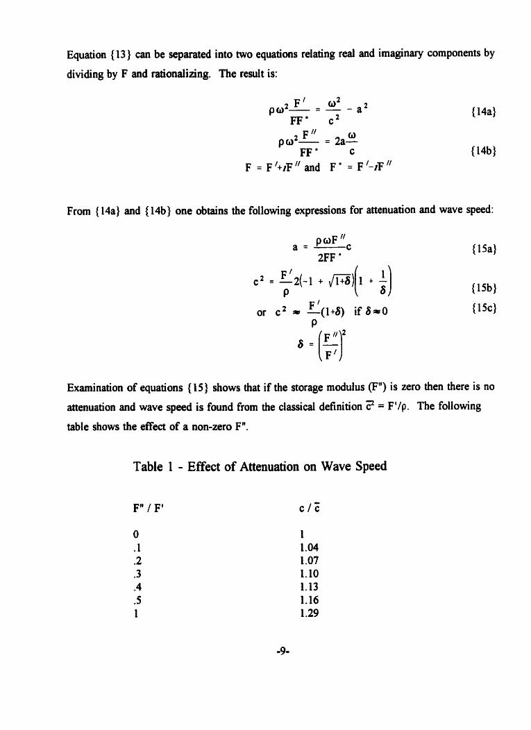
Examination of equations (15) shows that if the storage moduius (F") is zero then there is no

attenuation and wave speed is found from the classical definition ? = F'/p. The following

table shows the effect of a non-zero F".

Table 1 - Effect of Attenuation on Wave Speed

Obviously the effects of visco-elastic attenuation must be considered if materiai

stiffness is to be accurately calculated. Uafortwiately there is no simple way to measure

visco-elastic attenuation alone. This is due to the fact that the attenuation of an uitrasonic

wave in a FRP is due to several physical mechanisms, the dominant ones being transmission

(interface), scattering in addition to viscous loss. Scattering due to the distinct acoustic

properties of fibre and matrix are increasingly significant as the wavelength of the wave

approaches the fibre diameter.

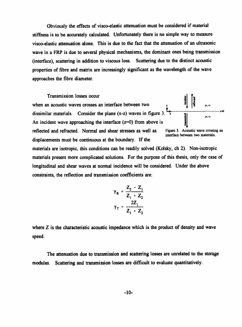
Transmission losses occur

when an acoustic waves crosses an interface between two z 4 - %=O dissimilar materials. Consider the plane (x-z) waves in figure 3. ' ; BI P. Q

An incident wave approaching the interface ( 24 ) from above is %I reflected and refracted. Nonnai and shear stresses as well as Figure 3. Acoustic wave ~0ss i -w

interface between two materiais. displacements must be continuous at the boundary. If the

materials are isotropic, this conditions cm be readily solved (Kolsky, ch 2). Non-isotropic

materials present more cornplicated solutions. For the purpose of this thesis, only the case of

longitudinal and shear waves at normal incidence will be considered. Under the above

constraints the reflection and transmission coefficients are:

where Z is the characteristic acoustic impedance which is the product of density and wave

speed.

The attenuation due to transmission and scattering losses are unrelateci to the storage

modulas. Scattering and transmission losses are difficult to evduate quantitatively.

"...use of attenuation as a characterization parameter has not been feasible due to the fact that it is affected by surfiace roughness and many other factors that are dificult to control." Mal and Ting, p. 21

Thus it is impractical to use the total measured attenuation in conjunction with measured wave

speed to evaiuate the complex material stiffiness. One alternative is to mechanically test

samples to obtain correction factors which can be applied to values calculated fiom wave

speed aione.

3.2 Acoustic wave in a fluid

During the early stages of curing, the thermoset will be a viscous fluid (a few

thousand centipoise is typical for low viscosity epoxies although some go as low as several

hundred cps. Water has a viscosity of 1 .O02 cps at 20 OC). Acoustic waves wül travel

through the fluid as either buk compressive waves (longitudinal) or as shear waves. A shear

wave will travel more slowly and will suffer more attenuation.

In the case of a fibre relliforced composite, the development of equations to describe

the waves propagation before gelation is daunting. Unlike the solid case, there is not a simple

method of lumping the matrix and fibre parameten. However, since the composite is

structurally useless when the maeix is uncured, quantitative evaluation of the material

properties are of littie value at that stage. What is important is that the attenuation of the

wave will be strongly dependent on the viscosity of the thennoset (especially for a shear

wave) - higher viscosity resuiting in lower attenuation. Monitoring the attenuation allows one

to estimate the rate of cure and the point at which gelation becomes complete. Thus

attenuation measurements - although of little use for calcuiating material properties (see 83.1)

- are of great qualitative value.

3.3 The Ultrasonic Transducer

A transducer is a device which converts energy fkom one form into another. In the

case of the ultrasonic transducer, mechanical waves are converted to electrical displacements

or vice versa. At the heart of an ultrasonic transducer is a piece of piezoelecûic material.

Piezoelectric is a term given to materials which, when defonned, produce a net electric

displacement.

3.3.1 Piezoelectric Materials

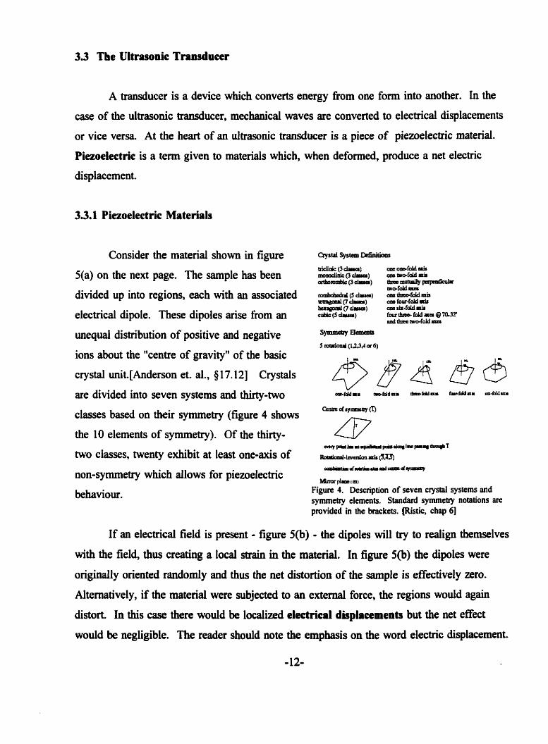
Consider the material shown in figure cqsui system ~ c ~ n i ~ i a r u

5(a) on the next page. The sample has been

divided up into regions, each with an associated

electrical dipole. These dipoles arise from an

unequai distribution of positive and negative

ions about the "centre of gravity" of the basic

crystal unit. [Anderson et. al., 8 1 7.121 Crystals

are divided into seven systems and thirty-two

classes based on their symmetry (figure 4 shows

the 10 elements of symmetry). Of the thirty-

two classes, twenty exhibit at least one-axis of

non-symmetry which allows for piezoelectric

behaviour . MLnrtdmim)

Figwe 4. Description of sevcn crystal systems and symmetry elements. Standard symmetry notations are provided in the brackets. [Ristic, chap 6]

If an electrical field is present - figure 5(b) - the âipoles will try to realign themselves

with the field, thus creating a local strain in the material. In figure 5(b) the dipoles were

originally oriented randomly and thus the net distortion of the sample is effectively zero.

Alternatively, if the material were subjected to an extemal force, the regions wodd agah

distoh In this case there would be localized electrical displacements but the net effect

wouid be negligible. The reader should note the emphasis on the word electric displacement.

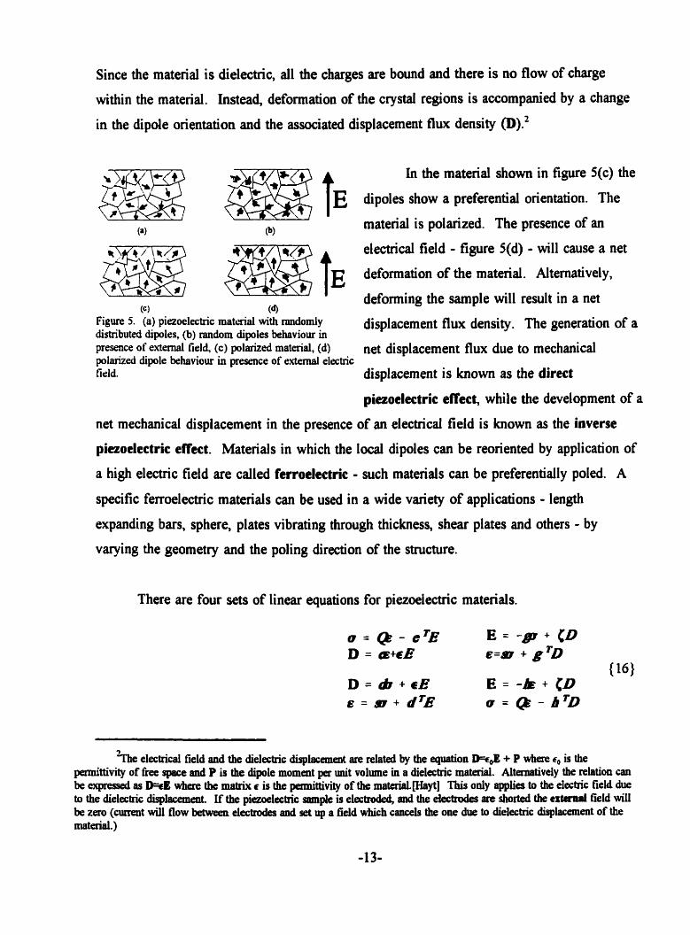
Since the matenal is dielectric, al1 the charges are bound and there is no flow of charge

within the material. Instead, deformation of the crystal regions is accompanied by a change

in the dipole orientation and the associated displacement fiw density

(Cf (4 Figure 5. (a) piezoelectric matmial with randomly distributed dipoles, (b) random dipoies behaviour in presence of e x t d field, (c) polarized material, (d) polarized dipole behaviour in presence of extemal electric field.

In the material show in figure S(c) the

dipoles show a preferential orientation. The

material is polarized. The presence of an

electrical field - figure 5(d) - will cause a net

deformation of the material. Altematively,

deforming the sample will result in a net

displacement flux density. The generation of a

net displacement flux due to mechanical

displacement is known as the direct

piezoelectric effect, while the development of a

net mechanical displacement in the presence of an electncal field is known as the inverse

pkzoelectric effect. Materials in which the local dipoles can be reoriented by application of

a high electric field are called ferroelectric - such materials can be preferentially poled. A

specific ferroelechic materials can be used in a wide variety of applications - length

expanding bars, sphere, plates vibrating through thickness, shear plates and others - by

varying the geometry and the poling direction of the structure.

There are four sets of linear equations for piezoelectric matenals.

'me electrical field and the dielechic displacement are related by the equation h , , E + P where q, W the pennittiviv of fkee pwe and P is the dipole moment per unit volume in a dielecüic material. Altenirttively the relation can be expressed as D=tE where the matrix r is the Wttivity of the material.[Nayt] This only applies to the elecûic field due to the dielectric displacement. If the piezoelectric sampk is elatroded, and the elecûades are shorted the cxtcrail field will be zero (current will flow between electrodes and set up a field which canceis the one due to dieIahic displacemat of the material,)

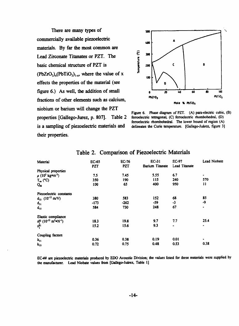
There are many types of

commercially available piezoelectric

materials. By far the most common are

Lead Sirconate Titanates or PZT. The

basic chernical structure of PZT is

(PbZrû,)x(PbTiO,), ., where the value of x

effects the properties of the material (see

figure 6.) As well, the addition of small

fiactions of other elements such as calcium,

niobium or barium will change the PZT

properties [Gallego-Jurez, p. 8071. Table 2

is a sampling of piezoelectric materials and

theu properties.

PeZrO, PbTiO,

Noie % PbliO3

Figure 6, Phase diagram of PZT. (A) para-electric cubic, (B) fcmIcctric terragond, (C) ferroelectric rhombohcdral, (D) ferroeltctric rhombohcdral. The lower bound of region (A) delincates the Curie temperature. [Gallego-Jutirez, figure 3)

Physical propcrtics p (10' kg*mS3) Ta (OC)

Qhl

Piezoclcctric constants dj3 (IO"* mN) 4 1

d t5

Coupling factors kir k33

Table 2. Cornparison of Piezoelectric Materials EC-65 EC-76 EC-3 1 EC-97 PZT PZT Barium Titanatc Lead Titanate

Lead Niobate

570 I l

85 -9

25.4 *

- 0.38

E C H am piezoekceic matcriah pmduccd by EW Acoustic Division; the values listed for rhese materiais w e n supplied by tfic manufacturer. tcad Niobate vducs h m [Gallego-fusvC& Table 11

An important parameter listed in Table 2 is the Curie temperature (TJ. Piezoelectric

ceramics properties are adversely affected by exposure to temperatures greater than Ta. For

some piezoelectric, exposure to temperatures above T, causes the crystal structure to change

to a symmetrical class which cannot support piezoelectric behaviour. In other rnaterials,

temperatures greater than the Curie temperature cause thermal agitation which "randombxs"

the distribution of regional dipoles [Anderson et al, p. 4691.

The mechanical quality factor QM, is a measure of the fiequency bandwidth of the

material. A high QM indicates a material which will only respond to a very narrow range of

fiequencies (electrical or mechanical) around its resonant fiequencies. k,, (lateral mode) and

k,, (thickness mode) are coupling factors - they indicate what fraction of electrical power is

transformed into mechanical power and vice versa. The coupling factors are not measures of

efficiency (recoverable energy over input energy), since some electrical power is capacitively

stored while some mechanical energy is elastically stored.

3.3.2 Broad-band Tiansducer Construction

There are a myriad of tmnsducer designs. For non-destructive *Dveld A

evaluation (N'DE) of materials, broad-band transducers are

favoured. The broad-band transducer is ideal for short pulse

applications. They are designecl to have as wide a fiequency response l a ~ v a band-width as possible, in order to obtain the maximum amount of

FiguR ,. Schematic of a

information. A typical broad band transducer (figure 7) has four geÏwal bmad band uansducer.

principal components.

The active component consists of an electroded plate of piezoelectric matenal.

Piezoelectrics with a low QM are desirable here. For low frequency applications the

electrodes have Little acoustic signincance. In high fieqwncy situations (greater than ten

MHz), where the wavelength is nmilar or d e r than the electrode thickness, the acoustic

effects of the electrodes must be accounted for.

One side of the active layer is baked with a highly attenuative material which has a

similar acoustic impedance to that of the piezoelectnc. This layer is responsible for damping

resonance in the pieu, as weil as lowering its QM and thus increasing the transducer's

bandwidth. Mixtures of epoxy and heavy metal powders (such as Tungsten) are used to

obtain bachg layers having the desired acoustic properties.

A matching layer is bonded to the opposite face of the piezoelectric plate for the

purpose of maximizing the energy transfer fiom the piezoelectric into the "target" material.

Maximum transmission of acoustic energy occurs when the acoustic impedance of the

matching layer is the geometric mean of the impedances of the piezoelectric and the target

materiai. Ideally the matching layer should be an integral multiple of the quarter wavelength

associated with the centre fiequency of the transducer.[Gailego-.luirez, p. 8 121 As weil, the

matching layer protects the piezoelectric material fiom Wear (principaily the electrodes.)

Manufacture of the matching layer can prove difficult (air entrapment at interface, temperature

effects etc.) and it is sometimes eliminated.'

A metal case around the backing layer and piezo-element completes the transducer.

The case is connected to the electrode on the emission face of the transducer and grounded,

thus creating a continuous "Faraday cagew4. Sensitivity to and emission of electro-magnetic

(EM) radiation is greatly reduced. This step is important for multiple transducers because the

inherent capacitance of the piezoelectric leads to strong EM coupling.

3Private conversation with Icff k W a l h m Canadian ND& Mississauga, Ont.

4~ metai shell is an equi-potennial surfacc - it does not producc a net ekcüic tield. IF elemenîs witb net electric fields were placed inside the sheli, an obsewer outside would only "see" sec the cqui-potcntial surface. The converse, an observer inside the shell and extemal fields, is also tme.

3.4 CMS Transducer Design Considentions

Design of the ultrasonic transducer(s) was hdamental to the effectiveness of the

CMS. To be useN the &ansducers had to be: physically small enough not to interfere with

the layup, able to withstand the heat of cure, able to generate and receive a measurable signal

through most of the cure cycle and inexpensive. Ideally the transducer's properties should

have k e n unaffected by temperature, so that the received signal was solely dependent on

changes in the curing composite's material properties.

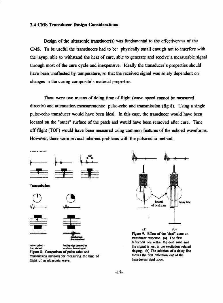
There were two means of doing t h e of flight (wave speed cannot be measured

directly) and attenuation measurements: pdse-echo and transmission (fig 8). Using a single

pulse-echo transducer would have been ideal. In this case, the transducer would have been

located on the "outer" surface of the patch and would have been removed after cure. Time

off flight (TOF) would have been measured using commoo featutes of the echoed waveforms.

However, there were severai inherent problems with the pulse-echo method.

Figure 8. Cornparison of pulpc-echo and fransmission mcîhods for measuring the time of flight of an ultrasonic wave.

ta) (b) Figure 9. Effect of the "deaf' zone on transducer rcsponse. (a) The first nflection lies within the deaf zone and ttie signai is lost in the excitation rclated cinging. (b) The addition of a delay line moves the fkt rcflecîion out of îhe tnuisducers deaf zone,

When pulsed, the active materiai of a transducer will "ring" at its resonant fiequency

for a few cycles. As long as the amplitude of the "ringing" exceeds that of received echoes,

the transducer is ineffective. Thus the transducer has a characteristic settiing time during

which usefùi data can not be obtained. If the settling time is multiplied by the characteristic

wave-speed(s) of the material being sampled, one recognizes that a "blind" - or more

accurately "deaf' - zone exists for the transducer. The standard solution to this problem is to

introduce delay ünes (an extra thick matching layer) which ensures that the material sampie

lies outside the deaf zone (see figure 9). Unfortunately, in the case of the CMS, addition of a

delay line would have made the transducer thicker and thus violated the srnall size

requirement. Another problem with pulse-echo occurs if the signal wavelength is relatively

short in which case, interfaces of plies of different orientations produce echoes which must be

accounted for.

The transmission method is not affected by problems listed above for the pulse-echo

method. However, the transmission method does require a pair of sensors, one of which is

embedded. As well, wave speed measurements are more difficult, and EM coupling between

the two tramducers must be deait with. The difficulty with TOF measurements results from

the need to distinguish between the "leading edge" of the acoustic wave, and noise (see $4.2

for m e r discussion.)

Transducers for the CMS required an operating temperature range between -25°C and

180°C The lower temperature was based on what might be experienced during a field repair

in mid-winter. Many commercial composites have cure temperatures as high as 180°C (350F)

which defined the upper limit of the operating temperature. A piezoelectric materiai which

did not undergo significant change in electro-mechanical properties within the operating

temperature range was desired. As well, other materials (e.g. adhesives, backing material,

solder) were restricted by temperature considerations.

4. The UTIAS Cure Monitoring System

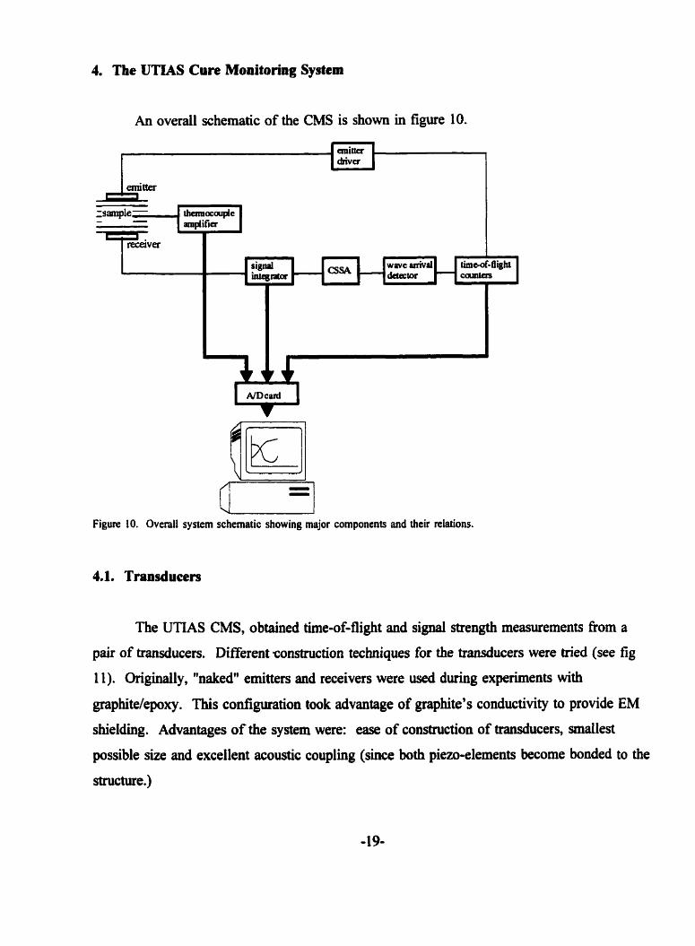
An overd schematic of the CMS is shown in figure 10.

n Figure 10. Ovenll system schematic showing major components and their relations.

4.1. Transducers

The UTIAS CMS, obtained time-of-flight and signal strength measurements fiom a

pair of transducers. Different ronstniction techniques for the transducers were tried (see fig

11). Originaily, "naked'' emitters and receivers were used during experiments with

graphite/epoxy. This configuration took advantage of graphite's conductivity to provide EM

shielding. Advantages of the system were: ease of construction of üansducers, mallest

possible size and excellent acoustic coupling (since both piezo-elements become bonded to the

structure.)

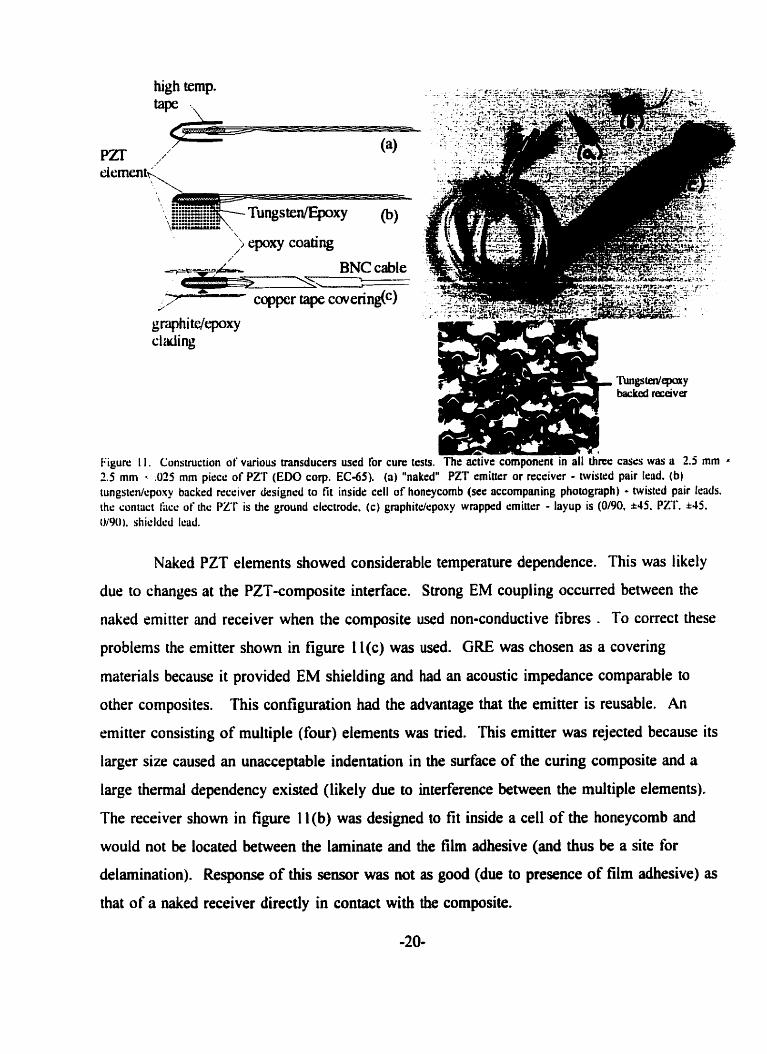
Naked PZT elements showed considerable temperature dependence. This was likely

dur to changes at the PZT-composite interface. Strong EM coupling occurred between the

naked rmitter and receiver when the composite used non-conductive fibres . To correct these

problems the emitter shown in figure 1 l(c) was used. GRE was chosen as a covering

materials becausc it provided EM shielding and had an acoustic impedance comparable to

other composites. This configuration had the advantage that the emitter is reusable. An

emitter consisting of multiple (four) elements was tried. This emitter was rejected because its

larger size caused an unacceptable indentation in the surface of the curing composite and a

large thermal dependency existed (likely due to interference between the multiple elements).

The receiver shown in figure 1 l(b) was designed io fit inside a ce11 of the honeycomb and

would not be located between the laminate and the film adhesive (and thus be a site for

delamination). Response of this sensor was not as good (due to presence of film adhesive) as

that of a naked receiver directly in contact with the composite.

The piezoelectric material used was EC-65 - made by EDO Acoustics it was a PZT

which was prirnarily designed for sonar type applications. It had a high piezoelectric

constant, relatively low QM, a hi& curie point and was inexpensive. One disadvantage of the

EC-65 was that its properties were strongly temperature dependent (a problem common to

PZT). Experiments were performed to characterize the overall thermal dependency of the

PZT (see section 5.1). An attempt was made at fmding a "correction factor"; the attempt was

unsuccessful due to interface effects which varied considerably fiom sample to sample.

Thin square pieces (.O25 mm x 2.5 mm x 2.5 mm) of the EC-65 were cut using a

dicing saw at Sunnybrook Health Sciences Centre. Based on these dimensions and the

material properties of the PZT, the expected principal frequencies were 7 MHz for the

thickness mode and 800 W for the lateral (planar) mode. The lateral mode (shear waves)

was the only mode used in experiments because it produced a stronger signal and offered

better attenuation response.

Leads were thin Kapton coated copper wire (magnet wire). The leads were attached

using a 93.5 Pb15 Sn/1.5 Ar rosin flux solder. Specified melting temperature of this solder

was 301 OC. A thin layer of epoxy was applied to the active electrode of the piezo-element to

provide electrical inmlation from the GRE covering.

4.2 Electronics

The major components of the CMS electronics were the emitter-àriver, the signal

integrator and the TOF circuitry. Schematics and system specification cm be found in

appendix A.

The emitter-driver was designed to excite the emitter element for a discrete number

(could be set fiom one to sixteen) of cycles at a constant frequency - the drive wave. This

method of driving the emitter maximized the amount of energy coupled into a specific

vibrational mode of the piezwlement. The emitter-driver was based on a Wien-bridge

-21-

oscillator [Sedra and Smith] which had a usefd fiequency range of approximately 400- 1 100

kHz. Power output per drive pulse could be adjusted via a large multi-turn potentiometer (P2

in figure A. 1) A crystal timer in the emitter-driver set the rate at which a dnve wave was

generated. The entire emitter-driver was switched on or off by the computer data-acquisition

systems.

Received waveforms passed through a band-pass filter to eliminate noise (high

frequency EM and low fkequency mechanical.) The band-pass filter was designed to

minunize the phase shift of the signal within a specific fiequency range and thus reduce

enors in the TOF measurement. Experimentally, the PZT elements used were found to have

their maximum response in the fkequency range of 700-900 kHz. Filters were designed to

give a maximum error of +/- 1 count (20 ns, see below) in the TOF circuit which meant a

maximum, absolute phase shifi of 5.0 deg and 6.5 deg at the low and high bounds

respectively of the aforementioned frequency range. A Butterworth bandpass filter with 3dB

points of 340 lrHZ and 1.8 MHz satisfied this constra.int. The filter is shown in figure A.2.

Signal strength measurement was obtained by amplifying, rectifying and integrating

(via successive low pass filters) the received signal. Figure A.2 shows the schematic of the

signai integrating circuit. Note that the fmal stage of the integrator has a time constant (b) of

22 ms (i.e. response rate limited by e'" where t, = 1/RC) Cure related changes in signal

strength were assumed to occur at a much slower rate than the limit of the integrator.

Experimental results c o n f i d this assumption (see 4 5.3.)

Three sub-systems constituted the TOF circuit - a constant signai strength amplifier

(CSSA), a wave arriva1 detector and a high speed (50 MHz) counter. Wave mival was

determined by the time at which the received signal first crossed a pre-set threshold voltage.

System noise restricted how low the detect threshold could be set. The CSSA was required to

prevent cure or temperature related changes in signal strength (which change the point at

which the wave crosses the detect threshold) fiom af5ecting TOF measurements. A

synchronization pulse fiom the emitter-driver started the TOF counters (figure A.4) advancing

when the drive-wave started. Wave arrival triggered a set of latches to obtain a "snap shot"

of the count. Ideally the 12 bit count should have been read directiy by the controllhg

cornputer. S b a digital data acquisition card was not readily available a DIA convertor was

used to provide an analog signal for the data acquisition card.

The temperature of the sample was measured using a thennocouple (T-type) which had

one junction embedded at the centre-line of the laminate and the other junction immersed in

an ice bath. A simple electronic circuit (figure A.6) was used to ampli@ the thermocouple's

voltage to a usehl level.

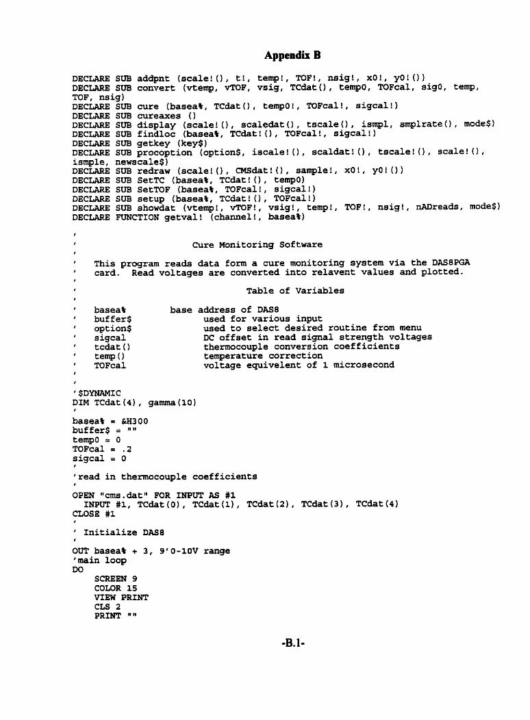
4.3 Cure Monitoring Software

Data fiom the CMS electronics was sampled with an analog to digitai data acquisition

card (Keithly Metrabyte DAS-8IPGA) in a 386 based PC. A simple program was written

which read data fiom the CMS and presented it in a graphical format. The program listing

can be found in Appendk B.

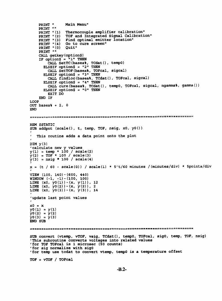
When monitoring a cure, the user could select a "sample period." The software always

accessed the A/D card at the maximum rate possible. However, data was averaged over the

sarnple period and only one value ploned and saved to file. For long cures (e.g. fibreglass

wet layup) a long sarnple period (10 or 30 seconds) was selected to avoid an excessively large

number of data points.

5. CMS Performance

Several cure tests were perfonned on various materials ranging fiom graphitelepoxy

prepregs to fibreglasdepoxy wet layups. Experiments indicated that the CMS produced usefùi

qualitative redts. The initial CMS design did not appear to have a satisfactory ability to

track the cure after gelation. However, the current CMS design showed considerable

potential, and can likely be developed into a commerciaUy viable prduct. Foliowing is a

detailed account of the primary problems and proposed corrections for the CMS.

5.1 Temperature Dependence

A significant problem with the CMS transducers was their strong temperature

dependence. Initially this problem was believed to lie principally with the PZT. Data sheets

for the materiai indicated that the fkequency constant and coupling factors were strongly

affected by temperature. Using data obtained during the cool d o m phase (when the material

should have been fully cured) of several cures an attempt was made at fmding temperature

correction factors for the PZT. It became apparent that the relation between signal strength

and temperature was anything but consistent; a result contrary to what would be expected if

the relation was mainly due to PZT materid properties (i.e. it is doubtfid that thermal

properties would Vary so drasticdly fiom PZT element to PZT element.) A reason for wide

variance in temperature dependency was that the emitter and receiver heated at different rates.

This differential heating would have to be accounted for in the correction factor - a very

cumbersome situation.

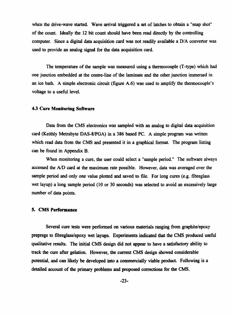
Several tests were performed to

examine the response of three different

emitterlreceiver combinations. Al1 tests

used the same receiver (a "naked PZT

wrapped in high temperature "flash breaker"

tape) under a cured (0194, +45a1 sample of

GRE. One emitter consisted of fou PZT

elements "wrapped" in GRE, another was

similar but with a single PZT element. The

third emitter consisted of a single PZT

element wrapped in a piece of high

temperature tape (similar to the receiver.)

* l ~ ~ ' - ' ~ ~ ~ ' L ' " ~ = - ' 1 .

20 # 40 50 60 70 80 40 100 110 1 -yiUi.rm

Figure 12. Temperature dependence of signal strength for three different emitters.

AU three emitters hzïd shielded leads. Molybdenum disulphide grease (chosen for availability

and high operational temperature) was used to improve transmission of waves into the ORE

samp1e. Signal strength versus temperature cuves for tfie three emitters is s h o w in figure

-24-

12. The c w e s show the relative performance of the emitters, they do not necessarily

represent the behaviour of a given emitter in an actual cure set-up. (The presence of the

moly-disulphide, which was not used duruig cure tests, created much Merent interface

conditions.)

The single element emitter with the GRE wrap had the best performance. This result

was likely due to improved coupling at the tramducerfsample interface. A notable difference

between the signal strength versus temperature occurred between wann up and cool down for

the single, GRE covered emitter. This result was likely due to temperature variations between

the emitter and receiver,

5.2 CMS Electronics Performance

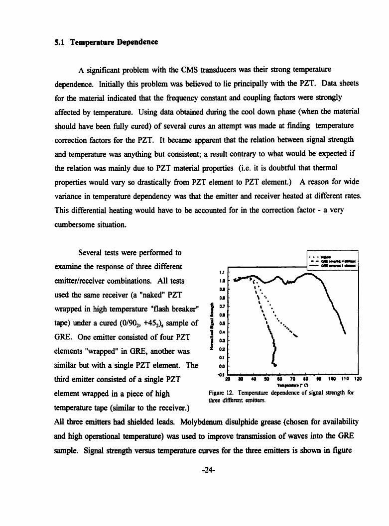
Tl-bW

Figure 13. Effect of signal changes on TOF. Initially the emitterdrivers powcr output was varied. Later the experimental setup was heated. The test used a pre-cured sample.

TOF measurements were found to be

unreliable. This was due to the nature of

the electronics. In the present system, the

ambient noise level was too high and prevented

accurate detection of the wave front.

Although the CSSA could compensate for

changes in the amplitude of a given

waveform, it could not adequately handle

changes in the achial wavefonn (see figure

13). Thus the leading edge of the wave

fiequentiy feil below the detector's

threshold. This problem could be resolved

by the introduction of several stages of

passive bandpass filters. Reducing noise wouid d o w the wave arriva1 threshold to be

lowered and thus accuracy improved. The CSSA could also be modified so that it would

maintain the leading edge of the wave at a constant amplitude.

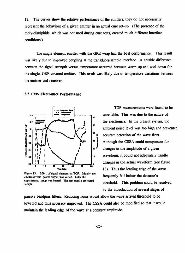
5.3 Qualitative Cure M o n i t o ~ g Using Signal Strength

Although the CMS did wt perform as well as desired, it did demonstrate great

potential. Figures 14(a)-(c) are plots of the normaüzed signai strength and cure temperature

versus time. The curves are consistent with what one would expect; decreasing signal

strength as the epoxy liquifies and then a (relatively) rapid increase at the tirne of gelation for

the pre-preg materials and a continuous increase in signal strength for the wet lay-up material.

Figure 14. Nonnalizeû signal striai& and tempeiature pmGies for seiezted cure tests. (a) (0/902, A45+ GRE (tested to Boeing spoc. BMSB- l68F) - n&ed emitkr and receiver; @) ( W b Kevlar/epay - naked exnitter, Tuq3ste4/epoxy backed &ver in hol~ycomb d l , (c) (û/90i, *Sz) glass/epairy wet layup wiog Pmet 1 2 5 D e p a ~ y system - GRE cwered, single elexnent emüter, naked nzeiver.

To ensure that the sudden increase in signal strength was indeed due to gelation and

not to other effects (e.g. temperature), a set of experiments was conducted. Several samples,

50 mm x 150 mm, (0/902+453S GRE - one of which was monitored by the CM$ - were

placed in an oven. These samples were cured for several hours to ensure they reached their

maximum expected properties. A second set of samples - one of which was again

inshymented - were also placed in the oven. However, in this case, the cure was stopped

mon afler the CMS indicated gelation was startiog. The cure was to have been stopped by

opening the vacuum bag and spraying water on the samples. However, when the bag was

opened it was discovered that the epoxy had not completely hardened - an observation clearly

indicating that gelation was occmhg but not complete. The samples were allowed to remain

in the oven for several extra minutes but were no longer under vacuum.

Fully cured (FC1 - FC4) and partially cured (PC1 - PC3) samples were trimmed, had

aluminum end tabs bonded on, and were then subjected tu tende testing. Table 3 lists the

samples' dimensions and failure loads. The ultimate stress for the partiaily cured samples

tended to be lower (average stress of 282 MPa) than for full cure samples (average stress of

378 MPa). Most noticeable was the mode of Mure. Al1 the Mly cured samples broke

through completely. The break lines were "clean", that is, Little delamination occuned. For

the partially cured samples, only the four 0190 plies failed. Extensive delamination was

observed at the interface between 0/90 and i45 plies. This type of failure clearly indicates

that the epoxy in the partial cure was indeed much weaker. One can thus appreciate the need

to maintain vacuum until gelation is complete. Photographs of the two modes of failure can

be found in figure 15.

Two m e r coupons (BGl and BG2) were given partial cures, this t h e with Bragg

grating fibre optic strain sensors embedded (55.4). Figure 16 shows the cure curves for the

two samples; their physical properties can be found in Table 3. After removal fiom the layup

it was obvious that the second sample was not cured properly - poking it proved the epoxy

was d l quite soft, while tapping it produced a dull sound, rather than the sharp one

consistent with fidl cures. The fist sarnple however appeared to be M y cured based on

visual inspection, tapping, poking etc. Mechanical tests quickly revealed that

neither sample had reached its optimum strength. Thus, the importance of the CMS is

apparent, especially in the case of the BG1 sample.

Table 3. Sample Properties

Sample Thic kness (mm) 1.74 1.73

Width (mm) 45.70 45.08 45 -27 46.00

Length Ultimate Load (kN) 30.3 33.6 29.2 25.9

Ultimate Stress (MPA)

381 43 1 373 327

Figure 15. (a) A selrction of tested GRE coupons. From lefi to right: partially cured sample (PC2). M y cured simple (FC3). Bragg p t i n g sarnple (BG2). (b) Sidr view of' partially cured sample (PC2) a h tensiie testing.

1.4 - 12 -

B ' * ; II O B -

:: = 0 . 2 -

09 -

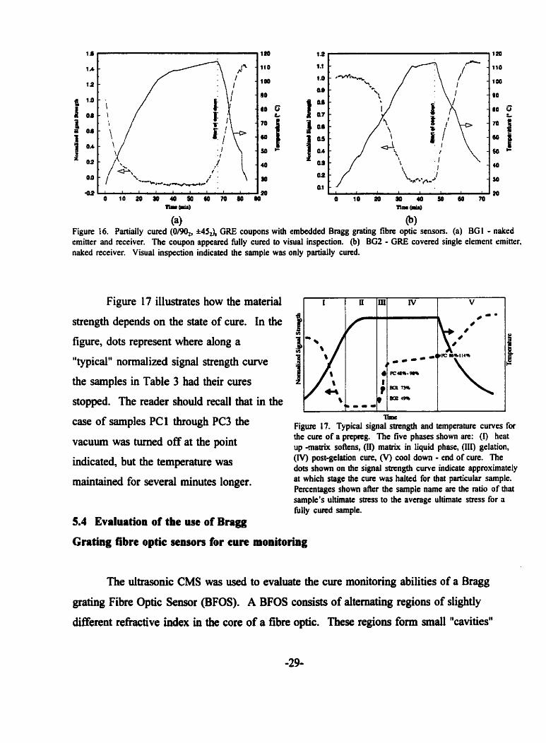
(a) @) Figure 16. Partially cured (0/90,, *45d, GRE coupons with embedded Bragg grating fibre optic sensors. (a) BGI - naked emitter and receiver. The coupon appeared hlly cured to visual inspection. (b) BG2 - GRE covered single etemcnt emitter, naked receiver. Visual inspection indicated the sample was only partiaHy cured.

Figure 17 illustrates how the material I I u m rv I v

strength depends on the state of cure. In the 1 0-• 0

figure, dots represent where dong a

"typical" normalized signal strength curve 4 KU*-ws

the samples in Table 3 had their cures

stopped. The reader should recall that in the @ Irn 49%

' .Da-

\ case of samples PCI through PC3 the

vacuum was tumed off at the point

indicated, but the temperature was

maintained for several minutes longer.

'Ibric Figure 17. Typical signal sucngth and temperature curves for the cure of a prcpreg. The five phases shown arc: (1) heat up matrix sokns, (II) matrix in liquid phase, (III) gelation, (IV) post-gelation cure, (V) cool down - end of cure. The dots shown on the signal strength curve indicate approximately at which stage the cure was halted for that particular sample. Perccntages shown a k r the samplc name are the ratio of that sample's ultimate stnss to the average ultimatc stress for a tùlly c w d sample.

5.4 Evaluation of the use of Bragg

Gratiiig fibre optic senson for cure monitoring

The ultrasonic CMS was used to evaluate the cure monitoring abilities of a Bragg

grating Fibre Optic Sensor (BFOS). A BFOS consists of alternathg regions of slightly

different refiactive index in the core of a fibre optic. These regions form srnail "cavities"

which selectively reflect a (ideally) single

fiequency of light. The wavelength (A) of the

reflected light varies with the length of the

"cavities". Thus, changes in the grating length

(strain) show up as shifts in A. If aii the

cavities undergo the same elongation (uniform

strain) the grating reflects a very narrow

bandwidth. In the case of a distributed strain a

A ibi

Figure 18. Distributed strain on a Bragg gnting fibre optic sensor. (a) A uniform strain is present dong the grating and aii the cavities reflect the same bandwidth. (b) In this case a distributed strain exists along the grating and the cavities reflect a spread of wavclengths.

larger range of fiequencies is reflected. This is shown in figure 18.

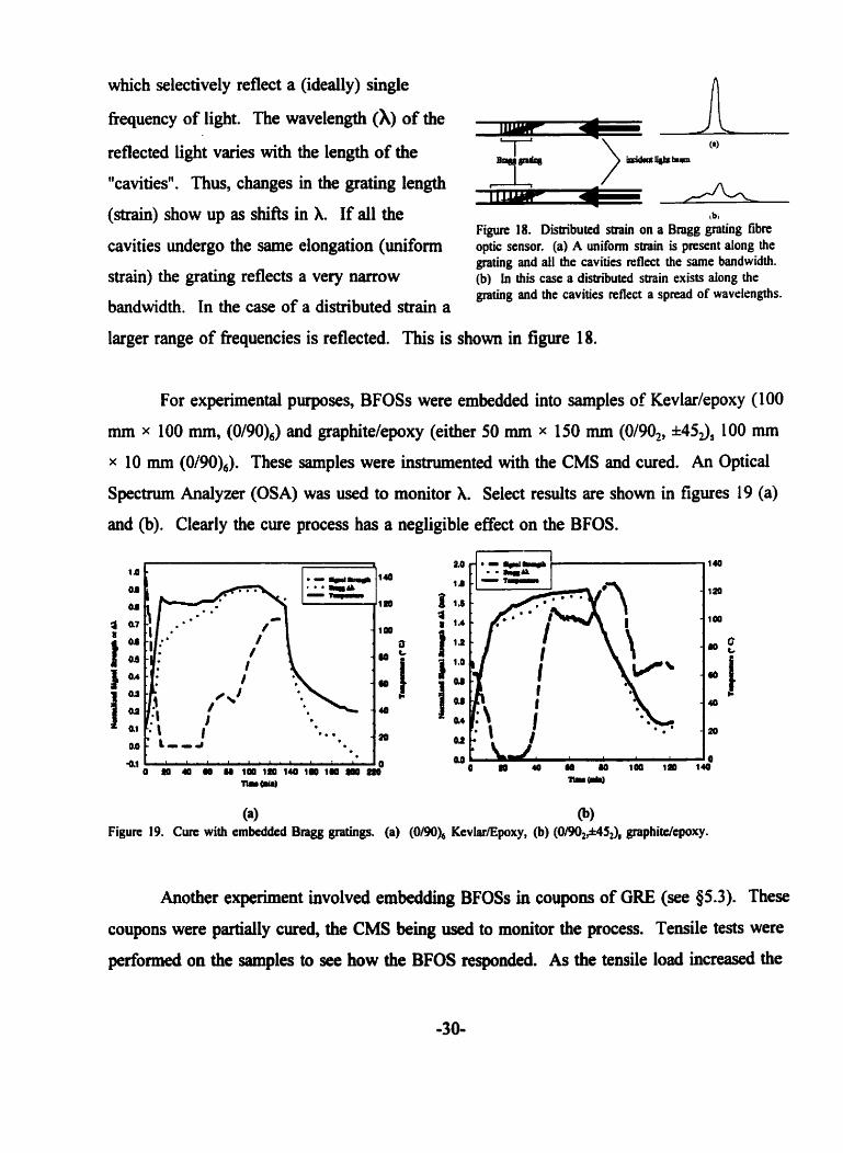
For experimental purposes, BFOSs were embedded into samples of Kevladepoxy (100

mm 100 mm, (0/90),) and graphitelepoxy (either 50 mm x 150 mm (()/go,, i453, 100 mm

10 mm (0/90),). These samples were instrumented with the CMS and cured. An Optical

Spechum Analyzer (OSA) was used to monitor A. Select results are show in figures 19 (a)

and (b). Clearly the cure process has a negligible effect on the BFOS.

Figure 19. Cure with embedded Bragg gratings. (a) (0/90), Kevlar~Epoxy, (b) (0190&453, graphitekpoxy.

Another experiment involved embedding BFOSs in coupons of ORE (see g5.3). These

coupons were partidy cured, the CMS king used to monitor the process. Tende tests were

perfomied on the samples to see how the BFOS responded. As the tende load increased the

BFOS showed a distributed strain (figure 20). It was apparent that the fibre optic was

slipping b i d e the material indicating epoxy failure. Note that the more Nly cured BG1

sample showed less strain distribution.

(a) @) Figure 20. Reflected spectruois at various tensile strains for GRE coupons with embedded bragg gratings. (a) BGl (b) BG2.

6. Conclusions

Although the UTIAS CMS, in its present fonn does not provide quantitative data on

the cure process, it does demonstrate considerable potentiai. Monitoring changes in signal

strength clearly provides qualitative data on when viscosity is at a minimum and when

gelation occurs. Qualitative data fiom the CMS will indicate if a composite which appears

Mly cured actually is not. Monitoring of pst gelation increases in material stifhess is not

dependable, a deficiency which cm be corrected with improved TOF measurements.

With a reasonable amount of effort, the wave-speed measurements could be made

reliable thus allowing the CMS to provide quantitative data during the entire cure process.

Future versions would use both longitudinal (thickness mode) and shear (lateral mode) waves

to obtain more detailed information on the material. The cunent CMS has already proved

useful in the characterization of the behaviour of Bragg grating fibre optic sensors embedded

in continuous fibre composites. Development of a commercidly viable product based on the

present design is a highly reaiistic possibility.

7. References

Anderson, J.C., K.D. Leaver, RD. Rawlings and J.M Alexander. Materials Science. 3rd Ed. Berkshire, UK: Van Nostrand Reinhold (UK) Co. Ltd, 1985.

Baker, A. A. "Repairs to Cracked or Defective Metallic Aircraft Components with Advanced Fibre Composites - O v e ~ e w of Austrdian Work." Cornpsite Structures 2, 1984. pp. 153- 181

Burkhardt, G. and N. Michacki. "Dielecûic Sensors for Low Cost Cure Control." 34th International SAMPE Symmsium and Exhibition, 1989. pp. 32-42

Chen, Li Che Ted. "A Unique Method of Determinhg the Elastic and Engineerllig Constants of Uni-directional Fibre-Reinforced Composite Plates using Ultrasound." University of Toronto Institute for Aerospace Studies R5274, Mar 199 1.

Chow, Andrea W. and Jack L. Bellin. "Simultaneous Acoustic Wave Propagation and Dynamic Mechanical Analysis of Curing of Thennoset Resins." Polymer Engineering and Science, 32(3), 1992. pp. 182-190

Crisicioli, P.R. and G.S. Springer. "Dielectric Cure Monitoring - A Critical Review." 34th International SAMPE Svmwsium and Exhibition, 1989. pp. 3 12-322

Crisicioli, P.R. and G.S. Springer. Smart Autoclave Cure or Comwsites. Lancaster, Pa: Technomic, 1990

Ellis, B. "Introduction to the Chernistry, Synthesis, Maaufacture and Characterization of Epoxy Resins" @p. 1-36) and "Kinetics of Cure and Network Formation" (pp. 72-1 16). Chemistw and Technoloev of Emxv Resins. Ed. B. Ellis, Glasgow, England: Biackie Academic 8t Professional, 1993.

Gallego-Juairez, J. A. "Piezoelectnc Ceramics and Ultrasonic Transducers. " Journal of Physics E: Scient@ Insîruments, 22, 1989. pp. 804-8 16.

Hahn, H.T. "Applications of Ultrasonic Technique to Cure Characterization of Epoxies." Non Destructive Methods for Materiai Pro~ertv Detelllljnation Ed. Clay Olaf Reud and Robert E. Green Jr. New York, USA: Plenum Press, 1984. pp. 315-326

Kolsky, H. Stress Waves in Solids. New York: Dover Publications Inc, 1963.

Md, A.K. and T.C.T. Ting. "Wave Propagation in Structural Composites" The Joint ASMWSES Appl. Mech and Eng. Sciences Conkence, Berkly Ca. Jn 20-22,

Measures, Raymond M. "Smart Composite Structures with Embedded Sensors," Composites Engineering, 2(5-7), 1992. pp. 597-6 18

Ohn, Myo Myint. "Fiber Optic Detection of Ultrasond and its Application to Cure Monitoring." Thesis M 437, University of Toronto, 1992.

Paik, Hyung-Jon and Nak-Ho Sung. "Fibre Optic Intrinsic Florescence for In-Situ Cure Monitoring of Amine Cured Epoxy and Composites." Poiymer Engineering and Science, 34(12), 1994. pp. 1025-1032

Perry, Mark J; James L. Lee and C. Williams Lee. "On-Line Cure Monitoring of EpoxyEraphite Laminates Ushg a Scaling Analysis and a Dual Heat Flux Sensor." Journal of Composite Materials, X(2). pp. 274-292

Ristic, Velimir M. Princioles of Acoustic Devices. Toronto, Canada: John Wiley and Sons, 1983.

Saliba, Susan; Tony Saliba and John F. L d a n e . "Acoustic Monitoring of Composite Materials During Cure Cycle." 34th International SAMPE Svmwsium and Exhibition. 1989, 1989. pp. 397-406

Sanjana, ZN. ''The use of microdielectronomy in Monitoring the Cure of Resins and Composites." Polynrer Engineering and Science, 26(5), 1986. pp. 373-379

Sedra, Adel S. and Kenneth C. Smith. Microelectronic Circuits. 2" Ed. New York: CBS College Publishing, 1987.

Skeist, Irving and George R. Sommerville. E-mxv Resins. New York, USA: Reinhold Publishing, 1962.

Sofer, G.A. and E.A. Hauser. Journal of Polymer Science, 13, 1952. p. 6 1 1

White, Scott R. "Ultrasound and Thermal Cure Monitor of an Epoxy Resin." 36th International SAMPE Smwsium and Exhibition, 199 1. pp. 284-297.

This appendix details the operation of each subsection of the CMS electronics.

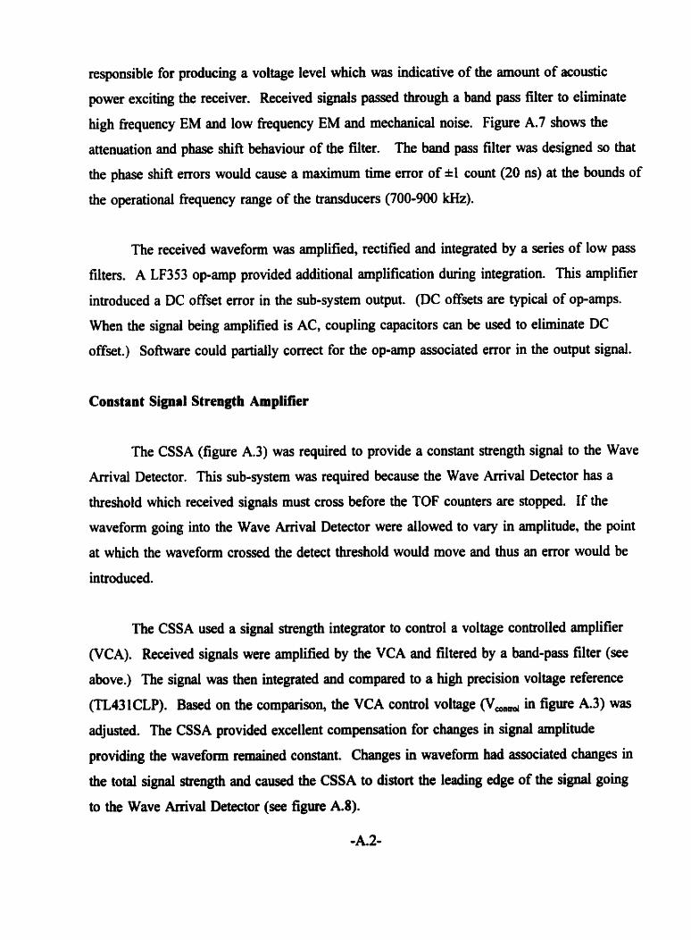
Emitter-Driver

The Emitter-Driver (figure A. 1) was responsible for exciting the emitter transducer. A

Wien-bridge oscillator (based around a LT1037 op-amp) coupled to a cycle counter was used

to generate discrete excitation wave forms of one through sixteen cycles at 400-1 100 kHz. A

programmable crystal oscillator (Statek PXO-1000) was used to maintain a constant rate of

excitation. Accurate output from the Signal Strength Integrator was dependant on a

consistent excitation rate. Digital control lines fiom the DAS-8 card in the PC would tum the

crystal timer on or off.

Dip switch DIPl was used to set the timer frequency (10 lrHz was standard) while

DIP2 was used to select the number of cycles (usually 3) in the excitation wave. The

frequency of the Wyne-bridge could be adjusted with potentiometer P l while the amplitude of

the excitation wave was varied with P2.

The cycle counter used a LM36 1 high speed (14 ns) comparator to detect when the

Wyne-bridge output crossed a threshold( which could be adjusted using P3). A 74AC169

binary counter would increment on the leading edges of the comparator output. As well, the

first "high" output fiom the comparator started the TOF counters advancing. The time

required for the excitation signal to first reach the detect threshold caused a small enor in

TOF measurements. This error could be adjusted to compensate for errors fiom the Wave

Arrivai Detector.

Signal Shrngth Integrator

Figure A.2 shows the Signal Strength integrator circuit. This sub-system was

responsible for producing a voltage level which was indicative of the amount of acoustic

power exciting the receiver. Received signals passed through a band pass filter to eliminate

high fiequency EM and low fiequency EM and mechanical noise. Figure A.7 shows the

attenuation and phase shift behaviour of the filter. The band pass filter was designed so that

the phase shift errors would cause a maximum the error of *1 count (20 ns) at the bounds of

the operational fiequency range of the transducers (700-900 kHz).

The received waveform was amplûied, rectified and integrated by a series of low pass

filters. A LF3 5 3 op-amp provided additional amplification during integration. This amplifier

introduced a DC offset error in the sub-system output. (DC offsets are typical of op-amps.

When the signal king amplified is AC, coupling capacitors can be used to eliminate DC

offset.) Software could partially correct for the op-amp associated error in the output signal.

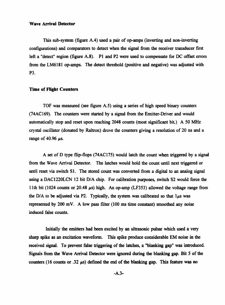
Constant Signal Strength Amplifier

The CSSA (figure A.3) was required to provide a constant strength signal to the Wave

Arrival Detector. This sub-system was required because the Wave Arriva1 Detector has a

threshold which received signals must cross before the TOF counters are aopped. If the

waveform going into the Wave Arrivai Detector were allowed to Vary in amplitude, the point

at which the waveform crossed the detect threshold would move and thus an error would be

introduced*

The CSSA used a signai strength integrator to control a voltage controlled amplifier

(WA). Received signals were arnplified by the VCA and filtered by a band-pass filter (see

above.) The signal was theo integrated and compared to a high precision voltage reference

(TL431CLP). Based on the cornparison, the VCA control voltage OI,, in figure A.3) was

adjusted. The CSSA provided excellent compensation for changes in signal amplitude

providing the waveform remained constant. Changes in waveform had associated changes in

the total signal strength and caused the CSSA to distort the leading edge of the signal gohg

to the Wave Amval Detector (see figure A.8).

Wave Arriva1 Detector

This sub-system (figure A.4) used a pair of op-amps (inverthg and non-inverting

configurations) and comparators to detect when the signal fiom the receiver transducer first

left a "detect" region (figure A.8). Pl and P2 were used to compensate for DC offset errors

fiom the LM61 81 op-amps. The detect threshold (positive and negative) was adjusied with

P3.

Time of Flight Counters

TOF was measured (see figure AS) using a series of high speed binary counters

(74AC169). The counters were started by a signai fiom the Emitter-Driver and would

automatically stop and reset upon reaching 2048 counts (most significant bit.) A 50 MHz

crystal oscillator (donated by Raltron) drove the counters giving a resolution of 20 ns and a

range of 40.96 p.

A set of D type flip-flops (74AC175) would latch the count when triggered by a signal

fiom the Wave Arrivai Detector. The latches would hold the count until next triggered or

until reset via switch SI. The stored count was converted fiom a digital to an analog signal

using a DACl22OLCN 12 bit DIA chip. For calibration purposes, switch S2 would force the

1 lth bit (1024 counts or 20.48 ps) high. An opamp (LF353) allowed the voltage range fiom

the DIA to be adjusted via P2. Typically, the system was calibrated so that lps was

represented by 200 mV. A low pass filter (100 ms t h e constant) smoothed any noise

induced faise counts.

Initially the emitters had been excited by an ultrasonic pulsar which w d a very

sharp spike as aa excitation waveform. This spike produce considerable EM noise in the

received signal. To prevent false triggering of the latches, a "blanking gap" was introduced.

Signals fiom the Wave Arrival Detector were ignored during the bl-g gap. Bit 5 of the

counters (16 counts or -32 ps) defined the end of the blanking gap. This feanire was no

longer needed with the current Emitter-Driver and with better shielded emitter traasducers.

Thermocouple Amplifier

Temperature measurements were taken using a T-type thermocouple embedded in the

laminates. A pair of op-amps (figure A.6) ampMed the thermocouple output approximately a

thousand times for use by the PC.

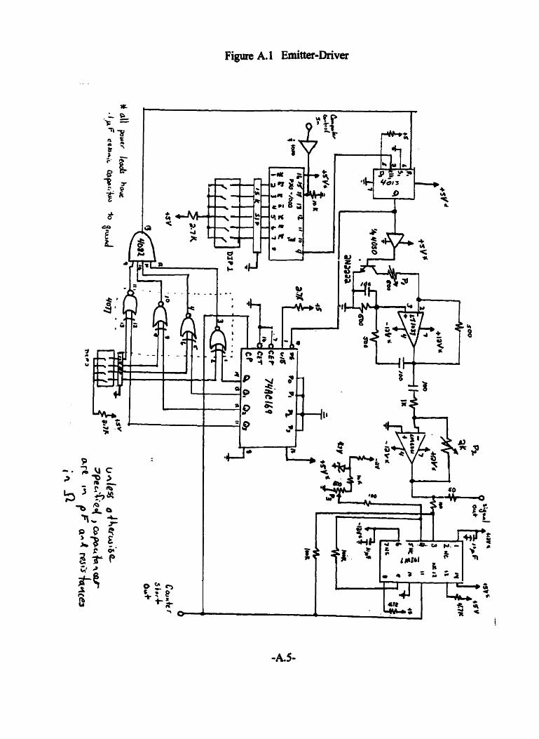
Figure A.1 Edtter-Driver

Fimire A.2 Signal Integrator and Band Pass Filters

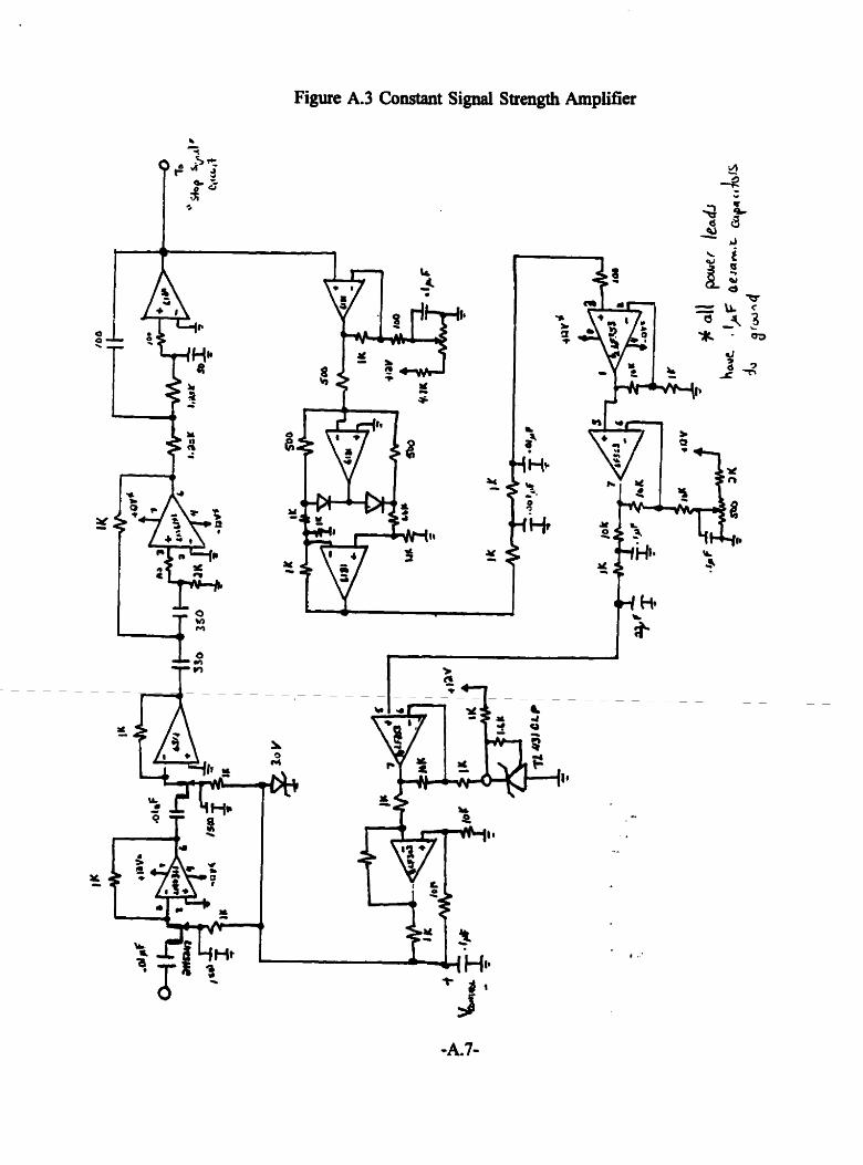
Figure A.3 Constant Signai Strength Amplifier

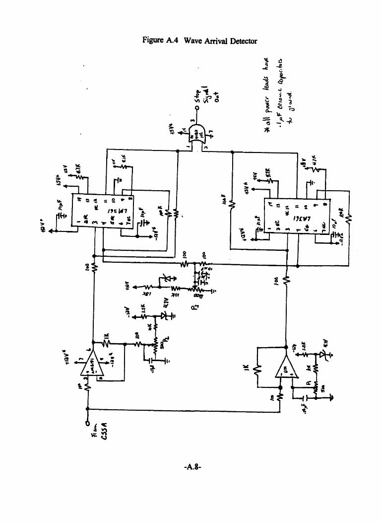
Figure A.4 Wave Amval Detector

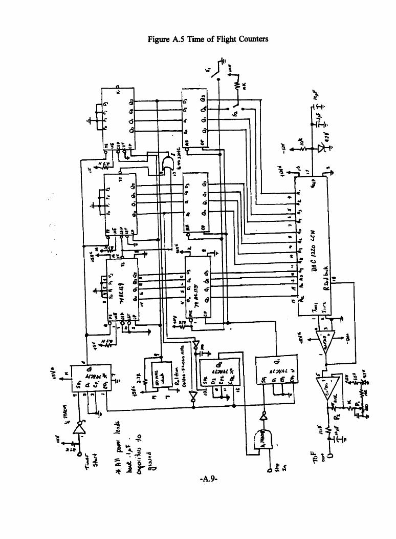
Figure AS The of Flight Counters

Figure A.6 Thennocouple Amplifier

Figure A.7 Aaenuation and phase shift of band-pass tilters. The fiiter was based on consecutive Buttenvorth high pass and low pass filters with 3dB points at 340 kHz and 1.8 MHz respectively..

received waveform CSSA output

Figure A8 Rcsponsc of CSSA to changes in meivecl signai. (a) reftrencc statt. (b) Signal amplitude changcd - CSSA compeosatcs and wave arrival tirne r-ns unchangcd. (c) Signal waveform changes - CSSA maintains intcgratcd signal strength. In this case the leading edge of the wave dccrrascs in amplitude and the wave arriva1 time is s W .

Appendu B

DECLARE SUB addpnt (scale! 0, t!, temp!, TOF!, nsig!, xO!, y0!0) D E C W SUE convert (vtemp, vTOF, vsig, TCdat (1 , tempo, TOFcal, sigo, temp TOF, nsig) DECLARE SOB cure (baseat , TCdat ( ) , tempo ! , T0Fcal ! , sigcal ! ) DECLARE SUE cureaxes ( 1 DECLARE SUE display (scale! ( ) , scaledat ( ) , tscale ( ) , ismpl , smplrate ( ) , mode$ ) DECLARE SUB findloc (baseat, TCdat!(), TOFcal!, sigcal!) DECLARE SUE getkey (key$ ) DECLARB SUE procoption (options, iscale! ( ) , scaldat ! 0 , tscale! ( ) . scale! ( 1 , ismple, newscale$) DECLARE SUE redraw (scale! ( ) , CMSdat ! ( ) , sample! , %O ! , y0 ! ( ) ) DECLiARE SUE SetTC (basea*, TCdat ! 0 , tempo) DECLARE SUB SetTOF (bases%, TOFcal!, sigcal!) DECLARE SUB setup (bases%, TCdat ! ( ) , TOFcal ! ) DECLARE SUE showdat (vtemp!, VMP!, vsig!, temp!, M F ! , nsig!, mreads, mode$) DECLARE FUNCTION getval! (chamel!. basealt)

Cure Monitoring Software

' This program reads data form a cure monitoring systern via the DAS8PGA card. Read voltages are converted into relavent values and plotted. '

Table of Variables

basea% base address of DAS8 buf fer$ used for various input option$ used to select desired routine from menu sigcal DC offset in read signal strength voltages tcdat0 thermocouple conversion coefficients tempo temperature correction TOFcal voltage equivelent of 1 microsecond

1

basea* = a300 buffer$ = tempo = O TOFcal = . 2 sigcal = O t

'read in thermocouple coefficients 1

OPEN "cms. dat" FOR INPUT AS #1 INPUT #1, TCdat (O) , TCdat (1) , T~dat (2 ) , ~ ~ d a t ( 3 ) , ~ ~ d a t (4 )

CLOSE #l 1

Initialize D E 8 t

OUT basea) + 3 , 9'0-1OV range 'main loop DO

SCREEN 9 COLOR 15 VïEW PRINT CLS 2 PR=

PRINT Main Menu" PRINT "" PRINT (1) Thenocouple amplifier calibration1I PRINT It (2) TOP and Integrated Signal Calibration" PRINT (3) Find optimal emitter locationIl PRINT " (4) Go to cure screentg PRINT (O) QuitN PRINT " " CALL getkey (option$) IF option$ = "118 THEN

CALL SetTC(baseat, TCdatO, tempo) ELSEIF option$ = I12l1 THEN CALL SetTOF (baseae, TOFcal , sigcal)

ELSEIF option$ = "3" THEN CALL findloc(baseat, TCdatO, TOFcal, sigcal)

ELSEIF option$ = I14l1 THGN CALL cure(basea%, TCdat(), tempo, TOFcal, sigcal, ngamnat,

ELSEIF option$ = #IOu THEN EXIT DO

EM3 I F LOOP OUT basea% + 2, O END

REM SSTATIC SUB addpnt (scale ( ) , t, temp, TOF, nsig, xO , y0 (1 )

' This routine adds a data point ont0 the plot /

D I M y ( 3 ) tcalculate new y values y(1) = temp * 100 / scale(2) y(2) = TOF * 100 / seale ( 3 ) y ( 3 ) = nsig 100 / scale(4) t

x = (t / 60 - scale (0) ) / scale(1) * 5,t/60 minutes / (minutes/div) * t

'update last point values t

SüB convert (vtemp, YK)F, vsig, TCdatO, tempo, TOPcal, sigo, temp, TOP, nsig) 'This subroutine converte voltages into related values for TOF TOFcal is 1 microsec (50 counts)

'for sig normalize with sigO ,for temp use tcdat to convert vtemp, tempo is a temperat- offset

TOF = vTOF / TOFcal

nsig = vsig / sigO temp = O FOR i = O TO 4 temp = temp + TCdat (i) * vtemp A i

NEXT i temp = INT(ternp * 10 + . 5 ) / 10 - tempo ' round to 1 decimal

END SUE

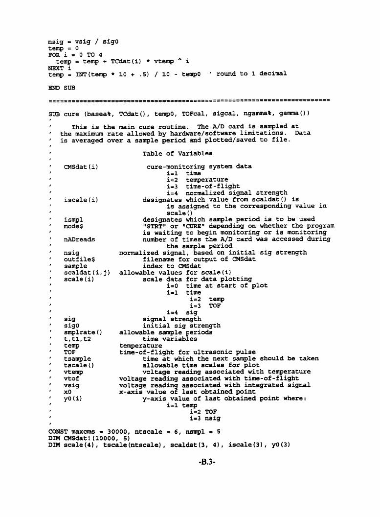
SU' cure (bases% , TCdat ( ) , tempo, TOFcal , sigcal , ngammaC . gamma ( ) 1

This is the main cure routine. The A/D card is sarnpled at the maximum rate allowed by hardware/software limitations. Data is averaged over a sample period and plotted/saved to file.

Table of Variables

CMSdat (i)

iscale (il

isrnpl mode$

ns ig outf ile$ sample scaldat (il j ) scale (il

sig sigo smplrate (1 t,tl, t2 t emp TOF tsample tscale ( ) vtew vtof vsig xo y0 (il

cure-monitoring system data i=i time i=2 temperature i = 3 time-of-flight i=4 nomlized signal strength

designates which value from scaldat0 is is assigned to the corresponding value in scale (1

designates which sample period is to be used 11STRTg8 or I~CORE~~ depending on whether the program is waiting to begin monitoring or is monitoring nurnber of times the A/D card was accessed during

the sample period normalized signal, based on initial sig strength

filename for output of CMSdat index to CMSdat

allowable values for scale(i) scale data for data plotting

i=O time at start of plot i=i time

2 temp i=3 TOF

i=4 sig signal strength initial sig strength

allowable sample periods time variables

temperature the-of-flight for ultrasonic pulse

time at which the next sample should be taken allowable time scales for plot voltage reading aasociated with temperature

voltage reading aasociated with tirne-of-flight voltage reading associated with integrated signal x-axis value of last obtained point

y-axis value of last obtained point where: i=l temp

i=2 TOF i d nsig

CONST maxcms = 30000, ntscale = 6, nsmpl = 5 DIM CMSdat! (10000, 5 ) DIM scale (4) , tscale (ntscale) , scaldat (3, 4 , iacale ( 3 ) , y0 ( 3 )

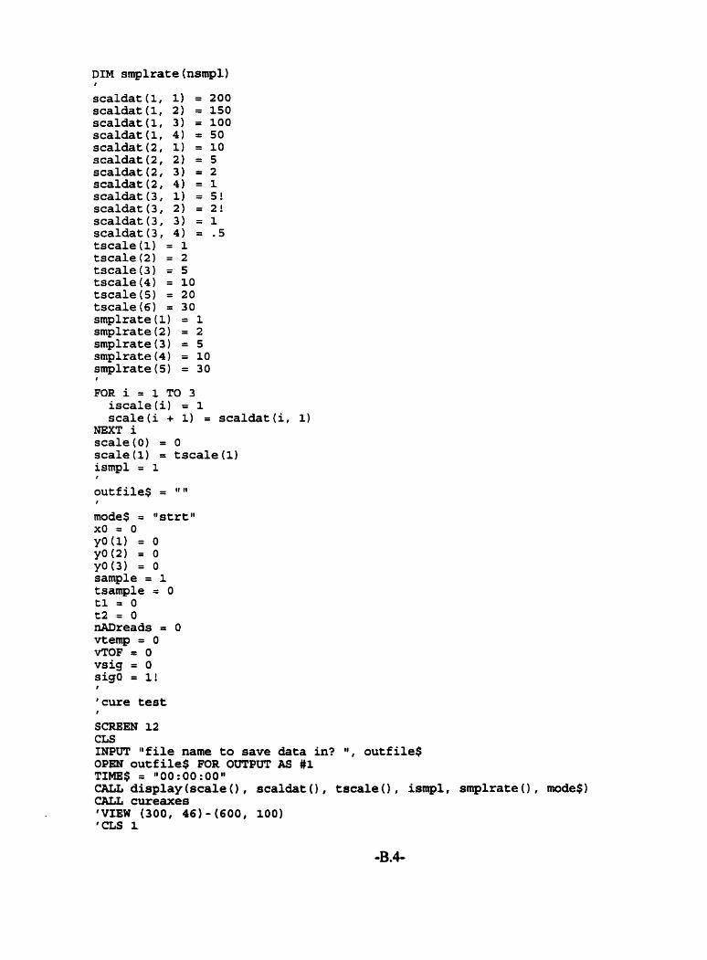
DIM smplrate (nsmpl) 1

scaldat(1, 1) = 200 scaldat(1, 2) = 150 scaldat (1, 3) = 100 scaldat (1, 4 ) = 50 scaldat(2, 1) = 10 scaldat(2, 2) = 5 scaldat(2, 3) = 2 scaldat (2, 4 ) = I scaldat(3, 1) = 5 ! scaldat(3, 2) = 2 ! scaldat(3, 3 ) = 1 scaldat(3, 4 ) = - 5 tscale(1) = 1 tscale (2) = 2 tscale (3) = 5 tscale (4 ) = 10 tscale(5) = 20 tscaïe(6) = 30 smplrate(1) = I smplrate (2) = 2 smplrate(3) = 5 smplrate ( 4 ) = 10 smplrate(5) = 30 I

FOR i = 1 TO 3 iscale (i) = 1 scale(i .t 1) = scaldat (il 1)

NEXT i scale(0) = O scale (1) = tscale (1) ismpl = 1 1

mode$ = "strtM xo = O yO(1) = O yO(2) = O yO(3) = O sample = 1 tsample = O tl = O t2 = O nADreads = O vtemp = O vTOF = O vsig = O sig0 = 11 1

'cure test f

SCREEN 12 CLS INPUT "file name to save data in? tu, outfile$ OPEN outfile$ FOR OUTPUT AS #1 TIMES = "00:OO:OO" CALL display (scale 0 , scaldat ( ) , tscale 0 , ismpl, CALL cureaxes 'VïEW (300, 46)- (600, 100) 'CLS 1

smplrate () ,

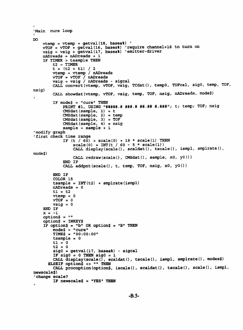
'Main cure loop 1

DO vtemp = vtemp + getval(l8, baseaib) ' vTOF = vTOF + getval(l6, basea8) 'require channel+l6 to turn on vsig = vsig + getval(l7, basea8) 'emitter-driver nADreads = nADreads .t 1 IF TIMER > tsample THEN

t2 = TIMER t = (t2 + tl) / 2 vtemp = vtemp / nADreads vTOF = vTOF / nADreads vsig = vsig / nADreads - sigcal CALL convert (vtemp, V M F , vsig, TCdat ( ) , tempo. ~OFcal, sigo, temp. M F .

nsig) CALL showdat(vtemp, vTOF, vsig, temp, TOP, nsig. nADreads. mode$)

IF mode$ = "curem THEN PRINT #I, USING v####.# ###.# ##.## #.###lu ; t; temp; TOP; nsig CMSdat (sample, 1) = t CMSdat(sample, 2) = temp CMSdat(sample, 3) = TOF CMSdat(sample, 4 ) = nsig sample = sample + 1

modiiy graph

END IF COLOR 15 tsample = INT (t2) + smplrate (ismpl) nADreads = O tl = t2 vtemp = O vTOF = O vsig = O

END IF x = -1 option$ = l u "

option$ = INKEY$ IF option$ = "bB1 OR option$ = llBM THEN

mode$ = lucurelt TIMES = "00:00:001~ tsample = O tl = O t2 = O sigO = getval(17, baseat) - sigcal IF sigO = O THEN sigO = 1 CALL display(aca1e ( ) , scaldat ( ) , tscale ( ) . ismpl, smplrate ( 1 , modes$)

ELSEIF option$ C> I g u 1 THBN CAU procoption (option$, iscale ( ) , scaldat () . tscale ( ) . scale (1 . ismpl,

newscale$) 'change scale?

IF newscale$ = nYEStl THESN ?

'need to check time range 1

'data scale toggle LOOP UNTIL option$ = fitqfi8 OR option$ = ItQt1

CLOSE #l

'Turn off emitter-driver OUT baseaO + 2 , O

END SUB

SUB cureaxes 1

This subroutine draws in the axes for the plot 1

VIEW (100, 140) - (600, 440) WINDOW - 1 , -1)- (100, 100) CLS 1 COLOR 15 LINE: (O, O) -(100, O) LINE (O, O) - ( O , 100) 1

FOR i = O TO 100 STEP 10 LINE (i, - 1 - , O ) LINE (i + 5, - 1 + 5, O) LINE - 1 , - 0 i)

NEXT i

END SUB

SUB display (~cale ( ) , scaldat ( ) , tscale ( ) , ismpl, smplrate ( 1 , mode$)

This routine displays the allowed and selected scales and sasnple rates as well as the allowed options

I

FOR i = l TO UBOUND(tsca1e) IF tscale(i1 = scale(1) THEN

iscale = i EXIT FOR

END IF NEXT i C

' d r a w in header

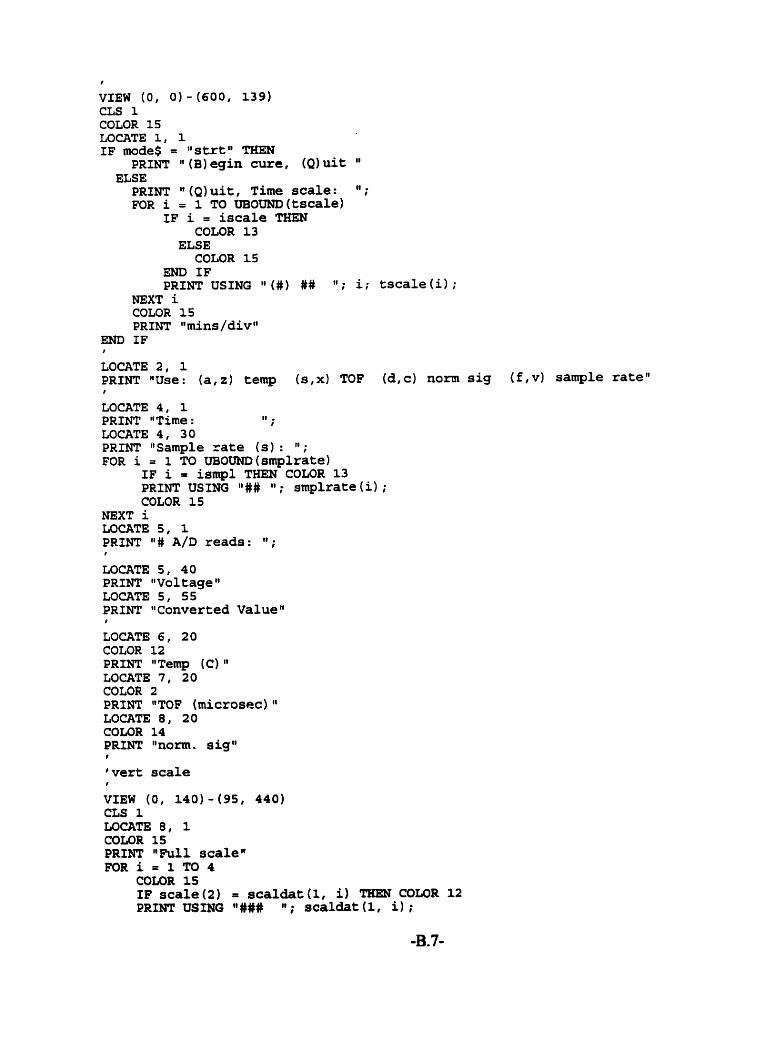
VIEW ( O , O ) - ( 6 0 0 , 139) CLS 1 COLOR 15 LOCATE 1, 1 IF mode$ = l1strtU THEN

PRINT IV (B) egin cure, (Q) uit ELSE

PRINT VQ)uit, Time scaie: Il;

FOR i = 1 TO ~ ~ ~ ~ ~ ~ ( t s c a l e ) IF i = iscale TEEN

COLOR 1 3 ELSE

COLOR 15 END IF PRINT USING (#) ## ; i; tscale (il ;

NEXT i COLOR 15 PRINT mmins/divfl

END IF 1

LOCATE 2, 1 PRINT 'IUse: (a, z) temp (s,x) TOP (d, c) nom sig ( f , v ) sample rateN

LOCATE 4 , 1 PRINT "Tirne : II I . LOCATE 4, 30 PRINT lisampie zate (s) : tt ; FOR i = 1 TO UBOUND(smp1rate)

IF i = ismpl THEN COLOR 13 PRINT USING I l # # I l ; smpïrate(i) ; COLOR 15

NEXT i LOCATE 5 , 1 PRfNT ln# A/D reads : ; 1

LOCATE 5, 40 PRINT VoltageM LOCATE 5, 55 PRINT "Converted Valueu I

LOCATE 6, 20 COLOR 12 PRINT ItTemp ( C ) IV LOCATE 7, 20 COLOR 2 PRINT "TOF (microsac) IV LOCATE 8, 20 COLOR 14 PRINT "nom. sig" 1

'vert scale 1

VIEW (0, 140)-(95, 440) CLS 1 LOCATE 8, 1 COLOR 15 PRINT V u l l scale It FOR i = 1 TO 4

COLOR 1s IF scale ( 2 ) = scaldat (1, i) THEN COWR 12 P R m US= "### l l ; scaldat(1, il;

COLOR 15 f F scale (3 ) = scaldat (2, i) THEN COLOR 2 PRZNT USING "## ; scaldat (2 , i) ; COLOR 15 IF scale ( 4 ) = scaldat (3, i) THEN COLOR 14 PRINT USING "#.#"; scaldat(3, i)

NEXT i 1

LOCATE 28 t 1 COLOR 12 PRINT " O " ; COLOR 2 PRINT lu O " ; COLOR 14 PRINT " 0 . 0 "

VIEW (0, 445) - (62% 465) CLS 1 COLOR 15 LOCATE 29, 10 PRZNT USING "####" ; scale ( 0 ) ; LOCATE 29, 40 PRINT "Tirne (min) " ; LOCATE 29, 75 PRXNT USING tQ####18; scale (0) + scale (1) 20;

END SUB

SUB f indloc (baseali., TCdat ( ) , TOFcal, sigcal) 1

* This routine is used to find the optimal location of the emitter by continuously monitoring signal strength and time-of-flight

t

iavg = 100 1

'start up CMS to allow system to stabalize vsig = getval(l6, bases%) SLEEP 2 ?

SCREEN 9 CLS 2 COLOR 15 LOCATE 1, 30 PRINT ugûptimal Transducer Locationm PRINT It "

PRINT "Place the emitter on the sample and slowly move it around." PRINT luUse the two bars to find the best position. fi

PRfNT lVPreas any key when done. l1 t

LOCATE 7 , 70 COLOR 2 PRINT "TOF" LOCATE IO, 70 COLOR 14 PRINT Vnt. Sigw VIEW (10, 80)-(510, 140) VIEW PRINT 14 TO 18 W I N D O W (O, 0)-(100, 3 ) t

TOF = O

vsig = O sigmax = O TOFmin = 10 option$ = It 1

DO 1

' draw boxes CLS 1 COLOR 15 LINE [ O , O ) -(lOO, O) LINE ( O , O ) -(O, 1) LINE (O, 1 - 0 1) LINE ( 100 , O ) - ( 1 0 0 , 1)

I

LINE (O, 2 ) - ( 1 0 0 , 2) LINE (O, 2 ) - (O , 3 ) LINE (O, 3 ) - ( 1 0 0 , 3) LINE ( 100 , 21 - ( 1 0 0 , 3 )

r

'draw in boxes 1

LINE (O, O ) - ( v s i g * 20 , l ) , 14, BF LINE (O, 2 ) - (TOF * 10, 3 ) , 2 , BF

' add max lines LINE (sigmax * 2 0 , O ) - ( s i g m a x * 2 0 + . 1 , l), 1 2 , BF LINE (TOFmin * 1 0 , 2) - (TOFmin * 1 0 + -1, 3 1 , 1 2 , BF

1

read in data 1

vsig = O TOF = O FOR j = 1 TO iavg

vTOFx = g e t v a l ( l 6 , baseae) vsigx = g e t v a l ( l 7 , baseat) CALL convert(0, vTOFx, v s i g x , TCdatO, O ! , TOFcal, I!, temp, TOFx, nsigx) TOF = TOF + TOFX vsig = vsig + vsigx

NEXT j TOF = TOF / iavg vsig = vsig / iavg - sigcal IF TOF < TOFmin THEN TOFmin = TOF I F vsig > sigmax THEN sigmax = vsig

1

CLS 2 LOCATE 14 , 28 COLOR 2 PRINT USING I l##. ### micro second^^^ ; TOF LOCATE , 28 COLOR 1 4

option$ = INKEXS LûûP UNTIL options O

OUT baseait + 2 , O

END SUB

S m getkey (key$) I

Wait for a key press and return the code for key I

key$ = " 1 '

DO WHILE key$ = key$ = -Y$

LOOP

END SüB

mJNCTION getval (channel, basea5) ?

This function reads the DASB card 1

Channel O - Time of flight Channel 1 - Integrated signal Channel 2 - temperature

1

16 is added t o the chamel to turn the emitter-driver of the electronics on

I

Input voltage ranges : 8 +/ - 10V sig, temp

9 10V TOI? f

IF channel = O OR channel = 16 THEN range = 9

ELSEIF channel = 1 OR channel = 17 range = 8

ELSEIF channel = 2 OR channel = 18 range = 8

ELSE P R m l1 * ERROR* ILLEGAL CHANNEL l1

STOP END IF f

OUT basea% + 3, range OUT baseat + 2, channel OUT base& + 1, O ?

DO status8 = INP(basea% + 2)

LOOP UNTIL statust < 128 1

IF range = O THEN getval = -5 + val0 10

ELSEIF range = 8 THEN getval = -10 + val0 * 20

ELSEIF range = 9 THEN getval = val0 * 10

END IF ?

END FUNCTION

sw procoption (option$, iscale ( ) , scaldat ( ) , tscale ( ) , scale ( ) , ismpl, newscale$) t

This subrouthe processes key presses which occur during the cure routine. 1

CONST nsmpl = 5 newscale$ = liNOM

IF option$ = "2" OR option$ = l lZ" THEN iscale(1) = iscale (1) + 1 IF iscale(1) > 4 THEN iscale(1) = 1 scale (2) = scaldat (1, iscale (1) ) newscales = "YESU

ELSEIF option$ = l'am1 OR option$ = "At1 THEN iscale(1) = iscale(1) - 1 IF iscale(1) < 1 THEN iscale(1) = 4 scale (2) = scaldat (1, iscale (1) ) newscales = "YES"

ELSEIF option$ = "xn OR option$ = "XM THEN iscale (2) = iscale (2) + 1 IF iscale ( 2 ) > 4 THEN iscale(2) = i scale (3 ) = scaldat (2, iscale (2) ) newscales = T E S u

ELSEIF option$ = "sW OR option$ = "Sll THEN iscale(2) = iscale(2) - 1 IF iscale (2) c 1 THEN iscale(2) = 4 scale ( 3 ) = scaldat (2 , iscale (2) ) newscales = "YESW

ELSEIF option$ = l@cN OR option$ = l8Clt THBN iscale(3) = iscale(3) + 1 IF iscale ( 3 ) > 4 THEN iscale (3) = 1 scale (4) = scaldat (3, iscale ( 3 ) ) newscales = "YES1'

ELSEIF option$ = lldtl OR option$ = I1D" THEN iscale(3) = iscale(3) - 1 IF iscale(3) < 1 THEN iacale(3) = 4 scale (4) = scaldat (3, iscale (3) ) newscales = "YEStf

?

'change sample rate? ELSEIF option$ = "v1' OR option$ = Vtl THEN isrnpl = ismpl - 1 IF ismpl c 1 THEN ismpl = nsmpl newscale$ = tlSMPLtl

ELSEIF option$ = "f l1 OR option$ = "FN THEN ismpl = ismpl + 1 IF ismpl > nsrnpl THEN ismpl = 1 newscale$ = ilSMPLtl

I

'change time scale? , ELSE x t = ASC (option$) - 48

IF x t >= 1 AND x t c üBOUND (tscale) TIlEN scale (1) = tscale (x*) scale(0) = O newscales = T B S "

END IF END IF

END SUB

SUB redraw (scale ( , CMSdat ( ) , sample, xO , y0 ( ) ) 1

Routine to redraw plot when scale data changed 1

'Since only 500 points can be drawn, the following routine 'selects only data points which roughly correspond to graphic points 1

'There are 25 graphics points per time division and scale(1) defines t h e number of minutes per time division 'Thus the number of seconds/graphic point is scale(1)*60/25 #

pnt = O tt = scale(1) * 2.4 ii% = i DO WHILE CMSdat (ii%, 1) < scale (O) 60

ii% = ii% + 1 LOOP 1

xO = (CMSdat (il% - 1, 1) / 60 - scale (O) ) / scale (1) * 5 ' t/6O minutes/(minutes/div) *5points/div

FOR i = ii% TO sarnpïe - 1 t = CMSdat(i, 1) IF INT((t - scale(0) * 60) / tt) > pnt THEN

temp = CMSdat(i, 2) TOF = CMSdatCi, 3 ) nsig = CMSdat(i, 4 ) cnsig = CMSdat(i, 5 ) CALL addpnt(scale0, t, temp, TOF, nsig, cnsig, xO, Y O O ) pnt = pnt + 1 IF pnt > 500 THEN EXIT FOR

END IF NEXT i

END SUB

Used to calibrate the thermocouple amplifier 1

iavg = 100 8

SCREEN 9 DO

COLOR 15, O CLS 2 LOCATE 1, 22 PRINT Valibrate Thermocouple Amplifier" PRINT "" PRINT I1(Q) t o quit, any other key to enter temperature offsetB8 PRINT "Current Off set : 81 ; P R m USING ll##.#ll; tempo COLOR 12 LOCATP: 6 , 22

PRINT "Temperature (C) ;

option$ = VIEW (290, 7 0 ) - ( 3 6 0 , 90) DO

CLS 1 LOCATE 6 , 40 P R I ~ US ING ### . # It ; temp ; temp = O FOR j = 1 TO iavg

vtemp = getval(2, baseat) tempx = O FOR i = O TO 4

tempx = tempx + TCdat(i) NEXT i

vtemp A i

temp = temp + tempx NEXT j temp = temp / iavg temp = INT(temp * 10 + - 5 ) / 10 - tempo option$ = ïNKEY$

LOOP UNTIL option$ c> IF option$ = "qn OR option$ = "QW THEN

EXIT DO ELSE COLOR 1 5 LOCATE 10, 1 INPUT "Enter new temperature offset ", tempo

END 1 F LOOP dummy = getval(2, basea8) END SUB

SUE SetTOF (basea*, TOFcal, sigcal) f

' This routine is used to set the voltage level associated with a TOF of 1 microsecond. As well, the DC offset in the signal strength is read.

#

iavg = 100 8

SCREEN 9 CLS 2 COLOR 15 LOCATE 1, 20 PRINT IlTime-of-Flight Circuit Calibrationw PRINT l1 'l

PRINT I l R e s e t flip-flops and set cal. switch offw PR= Wse zero adjust to zero system. Press any key when done" LOCATE 6, 16 COLOR 2 PRINT "TOF voltage "; option$ = VIEW ( 250 , 100) - (400, 110) DO

CLS 1 LOCATE 6, 34 PRINT WSING w##.###m; vTOF; vTOF = O FOR j = Z TO iavg

w = getval(0, baseat)

vTOF = vTOF + w NEXT j vTOF = vTOF / iavg option$ = -Y$

LOOP UNTIL option$ o I

CLS 2 COLOR 15 LOCATE 1, 20 PRINT "~ime-of-Flight Circuit CalibrationN PRINT "" PRINT luset cal. switch on. U s e gain adjust until voltage aprox 4.10 V . " PRINT "Press any key when doneu; LOCATE 6, 16 COLOR 2 PRINT "TOF voltage "; option$ = DO

CLS 1 LOCATE 6 , 34 PRINT USING "##.###"; vTOF; vTOF = O FOR j = 1 TO iavg

w = getval(0, baseab) vTOF = vTOF + w

NEXT j vTOF = vTOF / iavg option$ = INKEYS

LOOP UNTIL option$ c> TOFcal = 50 / 1024 * vTOF ' 5 0 counts is 1 microsecond I

COLOR 15 PRINT "If

PRINT " R e s e t TOF cal switchlt DO

w = getval(0, baseat) LOOP UNTIL w < 1 1

PRINT PRINT PRINT IVCalibrating Integrated Signal ..." PRINT sigcal = O nr = O tO = TIMER DO UNTIL (TIMER - t0) > 10 'sample for 10 seconds

sigcal = sigcal + getval(1, basea*) n r = n r + l

LOOP sigcal = sigcal / nr - -02 PR= "Integrated Signal offset: "; PRINT USING "#.###"; sigcal PRINT "based on "; nr; " A/D conversionsN PRIXT "Press any key to continue? option$ = DO option$ = INKEY$

LOOP üNTIL option$ c> r

END SUB

S W showdat (vtemp, YPOF, vsig, temp, TOP, nsig, nADreads, mode$) 1

This routine displays sead in voltages and their associated converted ' values. 1

VIEW (LOO, 5 0 ) - ( 2 0 0 , BO) CLS 1 VIEW (300, 8 0 ) - ( 6 0 0 , 130) CLS 1 1

COLOR 15 LOCATE 4 , 16 IF mode$ = ucureu THEN

PRINT TIMES ; ELSE

PRINT "XXXX" ; END IF 1

LOCATE 5, 16 PRINT USING If#####" ; nADreads ; I

COLOR 12 LOCATE 6 , 40 PRINT USING "##. ###If ; vtemp; LOCATE 6, 60 P R I ~ USXNG lm###.#"; temp #

COLOR 2 LOCATE 7 , 40 PRINT USING Il##. ###It ; vTOF; LOCATE 7 , 60 PRINT USING Il##.##"; TOF 1

COLOR 14 LOCATE 8 , 40 PRINT USING "##.###"; vsig; LOCATE 8 , 60 PRINT USING Il#.###"; nsig

END SUB