design and evaluation of tabu search algorithms for multiprocessor scheduling

P1: SAD

Journal of Heuristics KL604-03-Thesen June 23, 1998 16:37

Journal of Heuristics, 4: 141–160 (1998)c© 1998 Kluwer Academic Publishers

Design and Evaluation of Tabu Search Algorithmsfor Multiprocessor Scheduling

ARNE THESENDepartment of Industrial Engineering, University of Wisconsin—Madison, 1513 University Ave, Madison,WI, USA, 53706

Abstract

Using a simple multiprocessor scheduling problem as a vehicle, we explore the behavior of tabu search algorithmsusing different tabu, local search and list management strategies. We found that random blocking of the tail ofthe tabu list always improved performance; but that the use of frequency-based penalties to discourage frequentlyselected moves did not. Hash coding without conflict resolution was an effective way to represent solutions on thetabu list. We also found that the most effective length of the tabu list depended on features of the algorithm beingused, but not on the size and complexity of the problem being solved. The best combination of features includedrandom blocking of the tabu list, tasks as tabus and a greedy local search. An algorithm using these features wasfound to outperform a recently published algorithm solving a similar problem.

Key Words: tabu search, scheduling, performance evaluation

1. Introduction

Over the past 12 years, the tabu search has established its position as an effective meta-algorithm guiding the design and implementation of algorithms for the solution of largescale combinatorial optimization problems in a number of different areas (Glover (1986),Glover and Laguna (1997)). A key reason for this success is the fact that the algorithm issufficiently flexible to allow designers to exploit prior domain knowledge in the selection ofparameters and sub-algorithms. Such prior knowledge is frequently obtained by repeatedlysolving a few representative test cases using a spectrum of different techniques, attributesand/or parameters. Frequently referred to astarget analysis, an application of this learningapproach is described in Laguna and Glover (1993). In this paper we show that this approachcan be used to select and fine-tune sub-algorithms for a simple but still effective tabu searchalgorithm.

The problem of interest in this research is the multiprocessor scheduling problem. Briefly,this is the problem of assigningn independent tasks, each with a durationti (i = 1, . . . ,n),to m identical processors such that the completion time for the latest processor (i.e., themakespan) is minimized. The shortest schedule would be one where all processors com-pleted their work at the same time. The makespan of this schedule will be referred to as theideal schedule duration(T∗). T∗ is readily computed asT∗ = ∑ ti /m. The multiprocessorscheduling problem is a slight variation on the traditional bin packing problem where theobjective would be to find the number of processors needed to complete the project by agiven due date (Johnson et al. (1974), K¨ampke (1988)). The state-of-the-art of the use of

P1: SAD


142 THESEN

meta-heuristics to solve this class of problems is rapidly evolving. For an overview of re-cent contributions see Osman and Kelly (1996), and Glover and Laguna (1997). Overviewsof applications in the production scheduling area is given in Barness, Laguna, and Glover(1995) and Blazewicz et al. (1996).

The remainder of this paper is organized as follows: In Section 2 we introduce a num-ber of different sub-algorithms for managing and searching tabu lists. Among the topicsintroduced here are the use of hash coded tabus and the use of randomly blocked tabulist tails. In Section 3 we introduce and fine-tune eight different algorithms implementingdifferent combinations of the sub-algorithms introduced in Section 2. The performanceof the resulting algorithms is evaluated, and the best performer is identified. We will seethat, when task durations are expressed as three to four digit integers, a well-designed tabusearch algorithm can easily find the optimal solution to problems with up to 10,000 tasksand 500 processors. In Section 4 we evaluate the performance of the winning algorithmwhen solving more difficult problems. Results of a comparison with previously publishedresults for a related algorithm are also given. We will see that the best of the algorithmsdeveloped here used an average of about 60% fewer iterations to solve similar problems.Finally, a summary and conclusions are given in Section 5.

2. Elements of a tabu search

The tabu search algorithm combines a few simple ideas into a remarkably efficient frame-work for heuristic optimization. Among the main elements of this framework are:

• A (usually) greedy localsearch; the next solution is usually the best not-yet visitedsolution in the current neighborhood.• A mechanism (the tabu list) discouraging returns to recently visited solutions.• A mechanism that changes the solution path (perhaps by a random move) when no

progress has been made for a long time.

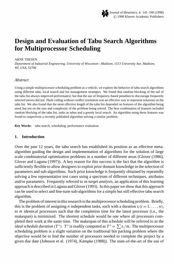
In addition, many tabu search algorithms incorporate other features such as flexiblememory structures and dynamic aspiration criteria (Glover (1995)). A rough overview of aconceptual tabu search algorithm is given figure 1. For difficult searches, techniques such asinfluential diversification (H¨ubscher and Glover (1994)) may be used to extend the durationand scope of the search.

Although a tabu search is conceptually simple, any implementation of an efficient tabusearch algorithm is problem specific, and no generic tabu search software is available atthis time. Among the issues faced by designers of tabu search algorithms are:

• The nature of the information included in the tabu list.• The way the tabu list is organized.• The lengths of the tabu lists.• The types of moves used to create new solutions.• The implementation of the local greedy search algorithm.• Strategies for diversifying the search when no progress has been made for a while.

P1: SAD


MULTIPROCESSOR SCHEDULING 143

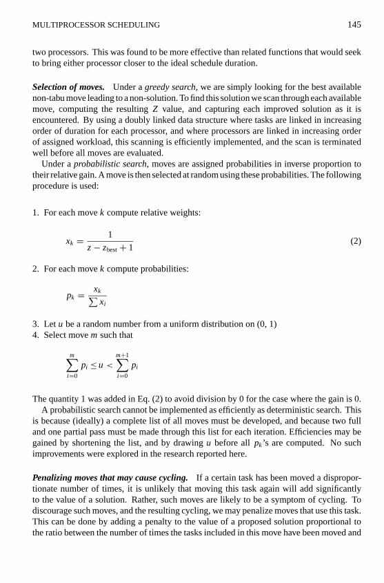
InitializeIdentify initial SolutionCreate emptyTabuListSetBestSolution=SolutionDefineTerminationConditionsdone=FALSE

Repeatif value ofSolution> value ofBestSolutionthen

BestSolution=Solutionif noTerminationConditionshave been metthen begin

addSolutionto TabuListif TabuListis full then

delete oldest entry fromTabuListfind NewSolutionby some transformation onSolutionif noNewSolutionwas foundor

if no improvedNewSolutionwas found for a long timethengenerate NewSolution at random

if NewSolutionnot onTabuListthenSolution= NewSolution

endelse

done=TRUEuntil done=TRUE

Figure 1. A rough overview of a conceptual tabu search algorithm.

In addition, many of the elements used in a tabu search are themselves heuristic algo-rithms, most of which rely on some carefully selected parameter value for optimal perfor-mance. Few generalizable guidelines are available for the choice of such parameters. Theseconcerns are discussed later in the paper. But first, let us review the main elements of thetabu search algorithm.

2.1. Solutions, moves and neighborhoods

Our strategy is to make successive changes to an initial solution such that a sequenceof improved solutions is obtained. Applying a commonly used strategy for combinatorialproblems that also was used by Barnes and Laguna (1993) and H¨ubscher and Glover (1994),we will use two types ofmovesto generate new solutions:

• Transfer: A task is assigned to another processor.• Interchanges: Two tasks performed by different processors are swapped.

Algorithms using transfers are simpler, and easier to implement, than those using in-terchanges. However, when a move is to be made between two processors performingn1

andn2 tasks respectively, the number of transfers available isn1+ n2, while the number ofinterchanges available isn1× n2. Given this larger number of choices, it is more likely thatthe interchange approach provides a better candidate for the next move. On the other hand,

P1: SAD


144 THESEN

interchanges do not change the number of tasks assigned to different processors. Hence, apure interchange-based algorithm is unlikely to find the optimum allocation of tasks. Wewill use a combined strategy that selects the best approach for each iteration. Barnes andLaguna (1993) noted that the use of two types of moves markedly improved the performanceof the search procedure. Our evaluations confirm this finding.

The set of new solutions that can be developed by a move from a given solution isreferred to as that solution’sneighborhood. A neighborhood hasn× (m− 1)members whentransfers are used. Hence, the local neighborhood can be quite large, and an exhaustivesearch of the entire neighborhood at every move is not feasible. Instead, we chose torestrict our search to moves between the busiest and the least busy processor. Since anymove reducing the project duration must reduce amount of work assigned to the busiestprocessor, this restriction does not reduce our ability to find a better solution (if one exists).

2.2. The local search

During the local search, the current neighborhood is explored, and a suitable move isselected. Ideally, all promising moves should be evaluated. But, for large neighborhoods,this may not be feasible. Instead, the search may be terminated as soon as a good moveis found. The criteria used in the local search may differ from the global criteria. Forexample, when looking for a job to transfer between two processors, let us look for the jobthat minimizes the difference in their total task durations. The search can be deterministicor probabilistic. In the first case, the best move is always picked. In the second case, a setof probabilities is computed from the values of all moves, and a move is selected at randomusing these probabilities.

Evaluation of moves. As a simplification, we consider only the effect that a move has onthe completion times for the busiest and least busy processor. In this case, the best moveis one where identical completion times are reached for the two processors. We measurethe value of a move by how far away the resulting latest completion time is away from thisideal time. Note that this completion time may not be the resulting project completion timeas another processor may take over the role as the busiest processor.

For an interchange, the value of a move is computed as the difference between theresulting latest completion time and the ideal completion time:

Zi j = Max{(db − tb,i + tl , j ), (dl + tb,i − tl , j )} − (db − dl )/2, (1)

where

dk = sum of durations of tasks assigned to processork,b = index of busiest processor (i.e.,db= max(dk), k= 1, . . . ,m),l = index of least busy processor (i.e.,dl = min(dk), k= 1, . . . ,m),

tk,i = duration of thei th task assigned to processork,Zi j = value of interchanging thei th task assigned to processorb with the j th

task assigned to processorl .Note that we seek to find a move that minimizes the difference in durations between the

P1: SAD



two processors. This was found to be more effective than related functions that would seekto bring either processor closer to the ideal schedule duration.

Selection of moves. Under agreedy search, we are simply looking for the best availablenon-tabu move leading to a non-solution. To find this solution we scan through each availablemove, computing the resultingZ value, and capturing each improved solution as it isencountered. By using a doubly linked data structure where tasks are linked in increasingorder of duration for each processor, and where processors are linked in increasing orderof assigned workload, this scanning is efficiently implemented, and the scan is terminatedwell before all moves are evaluated.

Under aprobabilistic search, moves are assigned probabilities in inverse proportion totheir relative gain. A move is then selected at random using these probabilities. The followingprocedure is used:

1. For each movek compute relative weights:

xk = 1

z− zbest+ 1(2)

2. For each movek compute probabilities:

pk = xk∑xi

3. Letu be a random number from a uniform distribution on (0, 1)4. Select movem such that

m∑i=0

pi ≤ u <m+1∑i=0

pi

The quantity 1 was added in Eq. (2) to avoid division by 0 for the case where the gain is 0.A probabilistic search cannot be implemented as efficiently as deterministic search. This

is because (ideally) a complete list of all moves must be developed, and because two fulland one partial pass must be made through this list for each iteration. Efficiencies may begained by shortening the list, and by drawingu before all pk’s are computed. No suchimprovements were explored in the research reported here.

Penalizing moves that may cause cycling.If a certain task has been moved a dispropor-tionate number of times, it is unlikely that moving this task again will add significantlyto the value of a solution. Rather, such moves are likely to be a symptom of cycling. Todiscourage such moves, and the resulting cycling, we may penalize moves that use this task.This can be done by adding a penalty to the value of a proposed solution proportional tothe ratio between the number of times the tasks included in this move have been moved and

P1: SAD


146 THESEN

the average number of times all parts have been moved:

Z∗i j = V + tb,i × nb,i

N+ tl , j × nl j

N(3)

where

Z∗i j = the modified value of the move,nk,i = count of moves for thei th task assigned to processork,

N= count of moves for all tasks.

UsingZ∗i j , in place ofZi j will encourage the exploration of other, possibly more promis-ing, areas of the solution space. One difficulty in using frequency-based penalties is that it isunclear what weight should be assigned to these penalties. On the other hand, Taillard (1994)reports on experiments where in every instance, it was possible to improve the efficiencyof a search by using frequency-based penalties. Our evaluations confirm this observation.However, for the algorithms evaluated here, each iteration became more time consuming,and no improvements in solution times were observed.

2.3. Tabus and tabu lists

A key premise of the tabu search is that usually it is better to visit new solutions than toreturn to recently visited ones. Toward this end, lists of recently visited solutions and/orrecently used moves are maintained. Moves are disallowed if they, or the solution they leadto, are found on these lists. Items placed on such atabu listremain there for a fixed numberof iterations (equal to the length of the list). For the present problem, let us explore the useof both solutions and task moves as tabus. We will see that there is a significant differencein performance between the two.

Tasks as tabus. The use of a task as a tabu has the advantage that a separate tabu list is notrequired. Instead, each task is marked by the time of its most recent move. This simplifiesimplementation. Reentry to a recently visited solution is now avoided by preventing tasksfrom being moved back to their previously assigned processor. However, the task is alsoprohibited from moving to other processors. This reduces the size of the neighborhood,and, perhaps, the efficiency of the search. Also, after a while, we may have moved all ofthe tasks assigned to a given processor to a different processor, potentially recreating a tabusolution using different processors. To avoid these situations, it is important not to restricttasks from being moved for too long.

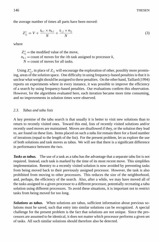
Solutions as tabus. When solutions are tabus, sufficient information about previous so-lutions must be saved, such that entry into similar solutions can be recognized. A specialchallenge for the present problem is the fact that solutions are not unique. Since the pro-cessors are assumed to be identical, it does not matter which processor performs a given setof tasks. All such similar solutions should therefore also be detected.

P1: SAD



1. For each processork compute:

sumsqk=nk∑

i=1

t2ki

where

tki =The i th task assigned to processorknk=Number of tasks assigned to processork

2. Sort processors such that:

sumsqi < sumsqj if i < j (i.e., processors are ordered by workload)

3. Compute the hash code:

h =m∑

k=1

k× sumsqk

where

h = Hash code value assigned to this solution

4. Placeh in a sorted list of hash codes. Markh by the time of insertion.

Figure 2. Hash coding scheme for tabu solutions.

For a large problem involving perhaps 10,000 tasks, and 1,000 processors, it is pro-hibitively expensive to store complete information about past solutions. Instead, let us usehash coding (Knuth (1973), Glover and Laguna (1997)) to reduce the relevant aspects ofprevious solutions to a single number. Now, an ordered list of hash codes, each representinga different tabu solution, can be constructed, and a search can easily be conducted to deter-mine if a proposed solution is on the list. Figure 2 presents the hash coding scheme used inthis study. Briefly, the hash code is computed as the biased sum of the sum-of-squares ofdurations of tasks assigned to individual processors. Although step 2 calls for processors tobe sorted in increasing order of assigned workloads, this step is not needed in practice. Thisis because processors already are ordered in this sequence to avoid having to deal with thelarge number of solutions that differs only in the identity of processors performing specificsets of tasks.

Note that no attempt is made to resolve conflicting hash codes (i.e., when differentsolutions are hashed to the same code). This is not a cause for concern when new entriesare added to the list, as the new entry simply replaces the old one. However, it may cause aproblem when a proposed solution is hashed to the same value as one obtained for a differentsolution currently on the list. In this case, the proposed new solution will erroneously berejected. However, the likelihood that two recent solutions have the same hash code is quitesmall; and, in our tests, computer programs dealing correctly with hash code collisions weresignificantly slower than those that did not. We will see that algorithms using hash-codedsolutions as tabus can be quite efficient, and that this efficiency is relatively insensitive tothe choice of tabu list length.

List length. The length of the tabu list(L), is a critical parameter in most tabu searchalgorithms. We will see that the wrong choice ofL may lead to a very inefficient algorithm.

P1: SAD


148 THESEN

Glover (1986) suggested that 7 would be a good value forL. Anderson et al. (1993) reportedthat list lengths between 7 and 15 worked well for a path assignment problem. Løkketangen(1995) cites a case where the most efficient algorithm included more than 200 items in thelist. Morton and Pentico (1993) suggest that keeping all solutions on the list works best forscheduling problems. Taillard (1994) reports on the successful use of lists that randomlychange in length at certain points of time. It appears that the most efficient length of thelist depends on the problem being solved, and the algorithm being used. In Section 3 weshow that long lists worked well for the test problems used here when solutions were tabus,while they were counter productive when tasks were tabus.

List tenure and blocking. Items usually stay on the tabu list for a number of iterationsequal to the length of the tabu list, and most algorithms consider an item to be a tabuthroughout its tenure on the tabu list. However, in some cases it is fruitful to make excep-tions. For example, H¨ubscher and Glover (1994) use a scheme where different portionsof the tabu list are blocked out (i.e., made inaccessible) at different times to encourageintensification and diversification. Here we will investigate a significantly simpler blockingscheme. Specifically, we introduce the concept of anaccessible listwith a random length(Ai ) that is established separately for each iteration. The accessible list is a subset of theentire list, and the entire list is maintained and updated as before. An item is considereda tabu for iterationi if it were given tabu status at iteration(i − Ai ) or later. At a lateriteration,Ai may have a smaller value, and an item previously considered to be a tabu, maynot be a tabu at this time. This approach differs from the periodically changing random listlengths used by Taillard (1994) in that a list of fixed length is always maintained, and thelength of the accessible subset of this list is reevaluated for each iteration.

The length of the accessible list for iterationi (Ai ) is a random quantity computed asfollows:

Ai = Alow + u× (Ahigh− Alow) (4)

where

Ai = length of the list accessible for thei th iteration,Alow= a constant giving the lower bound onAi ,Ahigh= a constant giving the upper bound onAi ,

u= random variable uniformly distributed between zero and one.

Extensive experiments have shown that the best value forAlow is one, and that the bestvalue forAhigh is L (the length of the list). We will see that the use of an accessible list ofrandom length improves the performance of all tabu search algorithms studied in this study.

2.4. Diversification

Occasionally, if the present solution path does not appear to be promising, it may be efficientto abandon the local search and to use a different mechanism to obtain the next solution.

P1: SAD



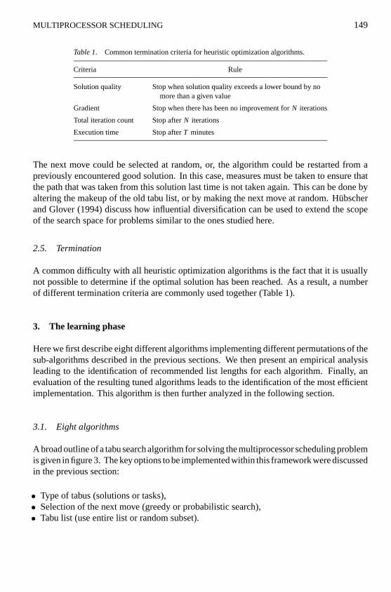
Table 1. Common termination criteria for heuristic optimization algorithms.

Criteria Rule

Solution quality Stop when solution quality exceeds a lower bound by nomore than a given value

Gradient Stop when there has been no improvement forN iterations

Total iteration count Stop afterN iterations

Execution time Stop afterT minutes

The next move could be selected at random, or, the algorithm could be restarted from apreviously encountered good solution. In this case, measures must be taken to ensure thatthe path that was taken from this solution last time is not taken again. This can be done byaltering the makeup of the old tabu list, or by making the next move at random. H¨ubscherand Glover (1994) discuss how influential diversification can be used to extend the scopeof the search space for problems similar to the ones studied here.

2.5. Termination

A common difficulty with all heuristic optimization algorithms is the fact that it is usuallynot possible to determine if the optimal solution has been reached. As a result, a numberof different termination criteria are commonly used together (Table 1).

3. The learning phase

Here we first describe eight different algorithms implementing different permutations of thesub-algorithms described in the previous sections. We then present an empirical analysisleading to the identification of recommended list lengths for each algorithm. Finally, anevaluation of the resulting tuned algorithms leads to the identification of the most efficientimplementation. This algorithm is then further analyzed in the following section.

3.1. Eight algorithms

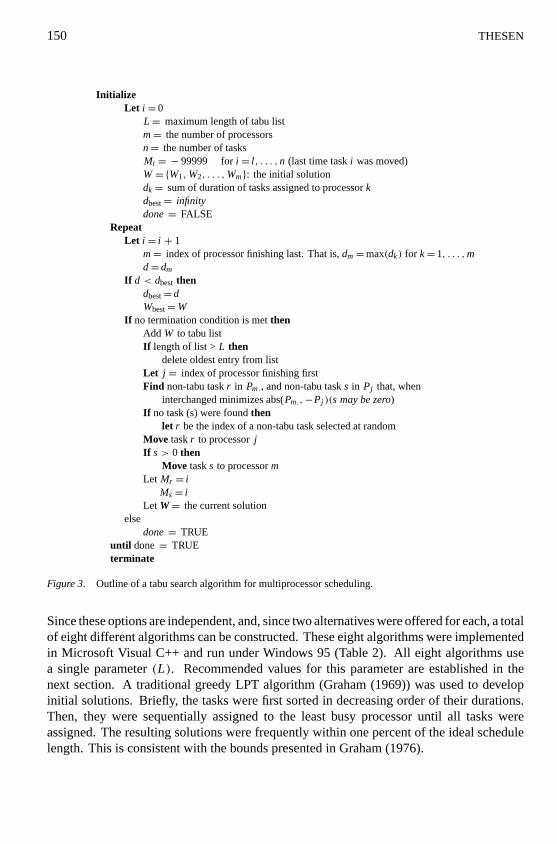
A broad outline of a tabu search algorithm for solving the multiprocessor scheduling problemis given in figure 3. The key options to be implemented within this framework were discussedin the previous section:

• Type of tabus (solutions or tasks),• Selection of the next move (greedy or probabilistic search),• Tabu list (use entire list or random subset).

P1: SAD


150 THESEN

InitializeLet i = 0

L = maximum length of tabu listm= the number of processorsn= the number of tasksMi = − 99999 fori = l , . . . ,n (last time taski was moved)W={W1,W2, . . . ,Wm}: the initial solutiondk= sum of duration of tasks assigned to processorkdbest= infinitydone= FALSE

RepeatLet i = i + 1

m= index of processor finishing last. That is,dm=max(dk) for k= 1, . . . ,md= dm

If d < dbest thendbest= dWbest=W

If no termination condition is metthenAdd W to tabu listIf length of list >L then

delete oldest entry from listLet j = index of processor finishing firstFind non-tabu taskr in Pm., and non-tabu tasks in Pj that, when

interchanged minimizes abs(Pm.,−Pj )(s may be zero)If no task (s) were foundthen

let r be the index of a non-tabu task selected at randomMove taskr to processorjIf s> 0 then

Move tasks to processormLet Mr = i

Ms= iLet W= the current solution

elsedone= TRUE

until done= TRUEterminate

Figure 3. Outline of a tabu search algorithm for multiprocessor scheduling.

Since these options are independent, and, since two alternatives were offered for each, a totalof eight different algorithms can be constructed. These eight algorithms were implementedin Microsoft Visual C++ and run under Windows 95 (Table 2). All eight algorithms usea single parameter(L). Recommended values for this parameter are established in thenext section. A traditional greedy LPT algorithm (Graham (1969)) was used to developinitial solutions. Briefly, the tasks were first sorted in decreasing order of their durations.Then, they were sequentially assigned to the least busy processor until all tasks wereassigned. The resulting solutions were frequently within one percent of the ideal schedulelength. This is consistent with the bounds presented in Graham (1976).

P1: SAD



Table 2. Eight different implementations of the tabu search algorithm givenin figure 2.

Algorithm Tabu Search Length of available tabu list

SGF Solutions Greedy Fixed= L

SGR Solutions Greedy Random=U(l, L)

SPF Solutions Probabilistic Fixed= L

SPR Solutions Probabilistic Random=U(l, L)

TGF Tasks Greedy Fixed= L

TGR Tasks Greedy Random=U(l, L)

TPF Tasks Probabilistic Fixed= L

TPR Tasks Probabilistic Random=U(l, L)

3.2. Searching for the best length of the tabu list

In order to explore the effect of the length of the tabu list(L) on performance, we measuredthe effort required by algorithms to solve thousands of random problems using differentvalues ofL. The resulting data was then analyzed for the purpose of finding the best(L∗)value of L for each algorithm. Particular attention was paid to the fact that the value ofL∗ might change with the size and complexity of the problem. Two types of analysis wereperformed:

• Graphical analysis, plots of solution times versusL were inspected for trends.• Nonlinear approximations, analytic functions were fitted and solved forL∗.

A random problem generator was used in all evaluations. This generator first producedthe requested number (between 500 and 10,000) of random task durations drawn from anexponential distribution with a mean of 1,000. These durations were then rounded up tothe next integer value. Finally, all durations were proportionally adjusted such that theaverage task duration was equal to the expected task duration. To ensure that a knownoptimal solution existed, the number of processors for each problem was set such that atleast 20 tasks were expected for each processor. Under these conditions, the ideal schedulelength was always reached. (More difficult problems including problems with uniformlydistributed, noninteger durations are evaluated in Section 4.)

Since optimal solutions were reached for all problems used in these evaluations, wewere able to adopt as performance measures both the time (in seconds), and the numberof iterations required to reach the optimal solution. In the remainder of this section therecommended list lengths for each algorithm are established. In the following section, weevaluate the performance of the resulting algorithms.

Graphical analysis. We first collected data on the time required by each algorithm to solve1,950 random problems, each with 5,000 tasks and 250 processors. All algorithms solved

P1: SAD


152 THESEN

Table 3. Effect of the length of the tabu list (L) on the time in seconds to solve problemswith 5,000 tasks and 250 processors. Random, integer processing times drawn from anexponential distribution were used. The optimal target solution was always found.

L TGR SGR SGF TGF TPR TPF SPR SPF

1 14.4 17.5 17.4 15.0 14.7 14.4 15.5 14.6

3 3.4 17.6 18.7 15.2 15.2 14.0 16.1 16.2

5 2.8 8.2 16.8 12.8 14.3 14.6 15.9 15.8

7 2.9 4.0 11.7 13.0 13.3 13.7 15.2 16.0

9 3.0 4.0 7.4 9.5 14.0 13.8 17.0 16.4

11 2.9 4.3 5.4 8.1 14.8 14.0 17.3 16.0

15 2.9 4.1 4.6 5.8 15.5 14.4 14.9 15.9

19 3.4 4.2 4.7 7.9 19.1 14.9 16.3 16.0

23 3.5 4.0 3.8 6.8 31.1 15.6 16.6 16.2

27 3.6 4.2 4.2 6.5 36.1 18.7 17.2 15.9

31 4.0 4.4 4.2 9.0 35.5 25.2 16.7 16.0

39 5.0 4.7 5.0 10.6 34.9 33.2 15.5 16.3

all problems. List lengths ranging from 1 to 39 were used. The results are summarizedin Table 3. We note that solution times for all greedy algorithms improved significantlyasL increased from one, while the solution times of the probabilistic algorithms improvedonly slightly if at all. In fact, the performance of SPR and SPF was found to be almostindependent ofL, and the performance of TPF and TPR deteriorated significantly asLincreased beyond 15. Table 3 also reveals that it is always possible to choose a valueof L for which a greedy algorithm performs significantly faster than its correspondingprobabilistic algorithm. It is interesting to note that TGR performed better than TGF forall values ofL. This was also true when runtimes were used as a performance measure.More research is required to explain this phenomenon. However, one possible explanationis that the random application of a shorter tabu list is sufficient to avoid cycling while at thesame time the (occasional) exploration of promising, but otherwise tabu, neighborhoods ispermitted.

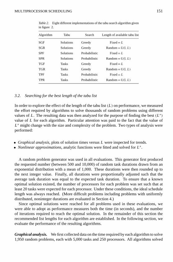
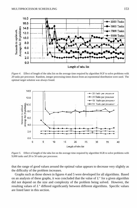
We then extended the analysis to problems with different numbers of tasks, but with thesame number of tasks per processors. Again, a large number of problems were generatedand solved using different algorithms and list lengths, and the resulting data sets analyzedin the same manner as in the previous section. A typical result for algorithm SGF withfrom 3,000 to 9,000 processors is shown in figure 4. We note that observed solution timesexhibit more variability as the size of the problem increases.

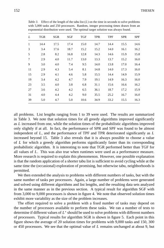
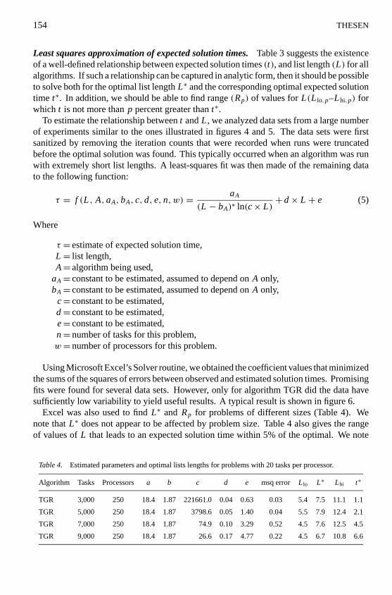
The effort required to solve a problem with a fixed number of tasks may depend onthe number of processors available to perform these tasks. We ran a number of tests todetermine if different values ofL∗ should be used to solve problems with different numbersof processors. Typical results for algorithm SGR is shown in figure 5. Each point in thisfigure shows the average of 20 solution times for problems with 9,000 tasks and 150, 300or 450 processors. We see that the optimal value ofL remains unchanged at about 9, but

P1: SAD



Figure 4. Effect of length of the tabu list on the average time required by algorithm SGF to solve problems with20 tasks per processor. Random, integer processing times drawn from an exponential distribution were used. Theoptimal target solution was always found.

Figure 5. Effect of length of the tabu list on the average time required by algorithm SGR to solve problems with9,000 tasks and 20 to 50 tasks per processor.

that the range of good values around the optimal value appears to decrease very slightly asthe difficulty of the problem increases.

Graphs such as those shown in figures 4 and 5 were developed for all algorithms. Basedon an analysis of these graphs, it was concluded that the value ofL∗ for a given algorithmdid not depend on the size and complexity of the problem being solved. However, theresulting values ofL∗ differed significantly between different algorithms. Specific valuesare listed later in this section.

P1: SAD


154 THESEN

Least squares approximation of expected solution times.Table 3 suggests the existenceof a well-defined relationship between expected solution times(t), and list length(L) for allalgorithms. If such a relationship can be captured in analytic form, then it should be possibleto solve both for the optimal list lengthL∗ and the corresponding optimal expected solutiontime t∗. In addition, we should be able to find range(Rp) of values forL(L lo,p–Lhi,p) forwhich t is not more thanp percent greater thant∗.

To estimate the relationship betweent andL, we analyzed data sets from a large numberof experiments similar to the ones illustrated in figures 4 and 5. The data sets were firstsanitized by removing the iteration counts that were recorded when runs were truncatedbefore the optimal solution was found. This typically occurred when an algorithm was runwith extremely short list lengths. A least-squares fit was then made of the remaining datato the following function:

τ = f (L , A,aA, bA, c, d, e, n, w) = aA

(L − bA)∗ ln(c× L)+ d× L + e (5)

Where

τ = estimate of expected solution time,L = list length,A= algorithm being used,

aA= constant to be estimated, assumed to depend onA only,bA= constant to be estimated, assumed to depend onA only,

c= constant to be estimated,d= constant to be estimated,e= constant to be estimated,n= number of tasks for this problem,w= number of processors for this problem.

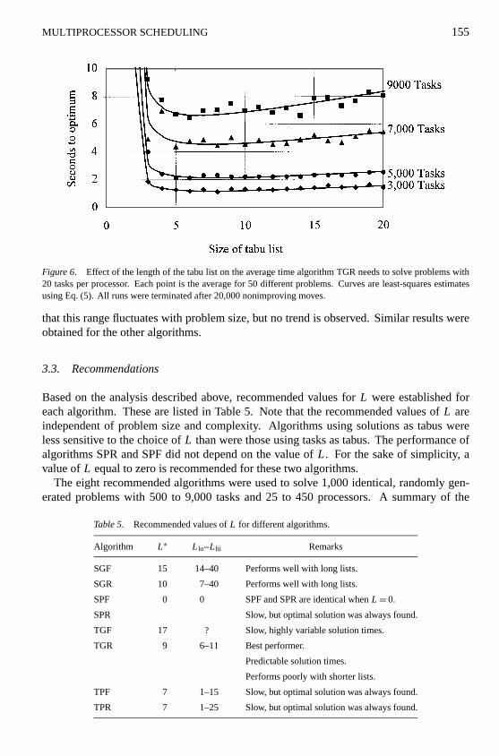
Using Microsoft Excel’s Solver routine, we obtained the coefficient values that minimizedthe sums of the squares of errors between observed and estimated solution times. Promisingfits were found for several data sets. However, only for algorithm TGR did the data havesufficiently low variability to yield useful results. A typical result is shown in figure 6.

Excel was also used to findL∗ and Rp for problems of different sizes (Table 4). Wenote thatL∗ does not appear to be affected by problem size. Table 4 also gives the rangeof values ofL that leads to an expected solution time within 5% of the optimal. We note

Table 4. Estimated parameters and optimal lists lengths for problems with 20 tasks per processor.

Algorithm Tasks Processors a b c d e msq error L lo L∗ Lhi t∗

TGR 3,000 250 18.4 1.87 221661.0 0.04 0.63 0.03 5.4 7.5 11.1 1.1

TGR 5,000 250 18.4 1.87 3798.6 0.05 1.40 0.04 5.5 7.9 12.4 2.1

TGR 7,000 250 18.4 1.87 74.9 0.10 3.29 0.52 4.5 7.6 12.5 4.5

TGR 9,000 250 18.4 1.87 26.6 0.17 4.77 0.22 4.5 6.7 10.8 6.6

P1: SAD



Figure 6. Effect of the length of the tabu list on the average time algorithm TGR needs to solve problems with20 tasks per processor. Each point is the average for 50 different problems. Curves are least-squares estimatesusing Eq. (5). All runs were terminated after 20,000 nonimproving moves.

that this range fluctuates with problem size, but no trend is observed. Similar results wereobtained for the other algorithms.

3.3. Recommendations

Based on the analysis described above, recommended values forL were established foreach algorithm. These are listed in Table 5. Note that the recommended values ofL areindependent of problem size and complexity. Algorithms using solutions as tabus wereless sensitive to the choice ofL than were those using tasks as tabus. The performance ofalgorithms SPR and SPF did not depend on the value ofL. For the sake of simplicity, avalue ofL equal to zero is recommended for these two algorithms.

The eight recommended algorithms were used to solve 1,000 identical, randomly gen-erated problems with 500 to 9,000 tasks and 25 to 450 processors. A summary of the

Table 5. Recommended values ofL for different algorithms.

Algorithm L∗ L lo–Lhi Remarks

SGF 15 14–40 Performs well with long lists.

SGR 10 7–40 Performs well with long lists.

SPF 0 0 SPF and SPR are identical whenL = 0.

SPR Slow, but optimal solution was always found.

TGF 17 ? Slow, highly variable solution times.

TGR 9 6–11 Best performer.

Predictable solution times.

Performs poorly with shorter lists.

TPF 7 1–15 Slow, but optimal solution was always found.

TPR 7 1–25 Slow, but optimal solution was always found.

P1: SAD


156 THESEN

Table 6. Mean and standard deviations of solution times and iterationcounts for optimized algorithms solving problems with 9,000 tasks and450 processors.

Iterations to optimum Seconds to optimum

Algorithm avg. stdv. avg. stdv.

TGR 2501 151.3 7.3 1.8

SGR 3150 584.2 10.1 2.5

SGF 3618 1101.8 11.1 3.5

TGF 15964 7724.1 25.5 12.0

TPF 5626 361.0 27.5 6.1

TPR 5447 396.3 29.1 6.2

SPF 4746 263.9 29.3 5.8

SPR 4745 275.9 29.7 6.2

resulting performance data for the case with 500 processors and 9,000 tasks is given inTable 6. Observe that algorithm TGR performed significantly faster and with significantlyless variability than all other algorithms. Similar results were observed for all other combi-nations of tasks and processors. We conclude that algorithm TGR with a list length equalto 9 is the best of the algorithms evaluated here.

4. Evaluation

In Section 3 we used test problems for which an optimal solution could always be found.This was done to simplify the process of fine-tuning sub-algorithms and identifying the bestcombination of features. Here we will evaluate the performance of the winning algorithm(TGR) when confronted with more complex problems. Since the value of the optimalsolution for these problems may not be equal to the ideal schedule duration(T∗), we willadopt a performance measure first used by H¨ubscher and Glover (1994). Specifically,the quality of the resulting solution will be measured as1T = (T − T∗)/T . First, wewill explore how the effort needed to solve a problem is affected by the precision of taskdurations. Then we will present a benchmark comparison between the effort expended byalgorithm TGR to solve random problems with durations in the range 0.0–1.0 and similarresults reported by H¨ubscher and Glover (algorithm HG). We will see that algorithm TGRdeals efficiently with more complex problems and that it terminates in fewer iterationsthan algorithm HG while reaching solutions of similar or higher quality. This performanceadvantage is particularly apparent for larger test problems.

4.1. Problem complexity

The number of potentially different solutions to a multiprocessor scheduling problem de-pends in part on the precision used to express task duration. A study was conducted todetermine how well the algorithm would perform when solving problems where task dura-tions are expressed with a higher degree of precision than the three to six digits used in the

P1: SAD



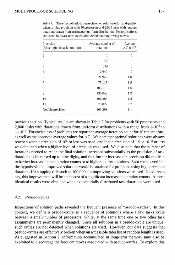
Table 7. The effect of task-time precision on solution effort and qualitywhen solving problems with 50 processors and 2,000 tasks with randomdurations drawn from an (integer) uniform distribution. Ten replicationsare used. Runs are terminated after 20,000 nonimproving moves.

Precision Average number of Average(Max digits in task duration) iterations 1T × 108

2 1 0

3 27 0

4 314 0

5 2,649 0

6 24,943 1.0

7 75,115 1.9

8 103,110 1.6

9 135,043 1.2

10 106,285 1.3

11 79,027 0.7

Double precision 103,291 1.1

previous section. Typical results are shown in Table 7 for problems with 50 processors and2,000 tasks with durations drawn from uniform distributions with a range from 1–102 to1–1011. For each class of problems we report the average iteration count for 10 replications,as well as the observed average values for1T . We note that optimal solutions were alwaysreached when a precision of 105 or less was used, and that a precision of 1.9× 10−8 or lesswas obtained when a higher level of precision was used. We also note that the number ofiterations needed to reach the final solution increased substantially as the precision of taskdurations is increased up to nine digits, and that further increases in precision did not leadto further increase in the iteration counts or to higher quality solutions. Spot checks verifiedthe hypothesis that improved solutions would be attained for problems using high precisiondurations if a stopping rule such as 100,000 nonimproving solutions were used. Needless tosay, this improvement will be at the cost of a significant increase in iteration counts. Almostidentical results were obtained when exponentially distributed task durations were used.

4.2. Pseudo-cycles

Inspections of solution paths revealed the frequent presence of “pseudo-cycles”. In thiscontext, we define a pseudo-cycle as a sequence of solutions where a few tasks cyclebetween a small number of processors, while, at the same time one or two other taskassignments are permanently changed. Since all solutions in a pseudo-cycle are unique,such cycles are not detected when solutions are used. However, our data suggests thatpseudo-cycles are effectively broken when an accessible tabu list of random length is used.As suggested in Section 2, information accumulated in long-term memory may also beexploited to discourage the frequent moves associated with pseudo-cycles. To explore this

P1: SAD


158 THESEN

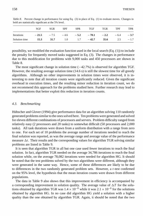
Table 8. Percent change in performance for using Eq. (3) in place of Eq. (1) to evaluate moves. Changes inbold are statistically significant at the 5% level.

SGF SGR SPF SPR TGF TGR TPF TPR

Iterations − 21.5 − 7.5 − 4.6 − 5.2 − 70.1 − 2.2 − 6.4 − 3.7

Solution time 15.3 31.7 1.0 1.7 − 42.7 35.6 2.5 − 1.7

possibility, we modified the evaluation function used in the local search (Eq. (1)) to includethe penalty for frequently moved tasks suggested in Eq. (3). The changes in performancedue to this modification for problems with 9,000 tasks and 450 processors are shown inTable 8.

The most significant change in solution time (−42.7%) is observed for algorithm TGF.However, the resulting average solution time (14.6 s) is still the slowest time for all greedyalgorithms. Although no other improvements in solution times were observed, it is in-teresting to note that all iteration counts were significantly reduced. Given the significantoverhead in execution times, and the resulting minor reduction in iteration count, we donot recommend this approach for the problems studied here. Further research may lead toimplementations that better exploit this reduction in iteration counts.

4.3. Benchmarking

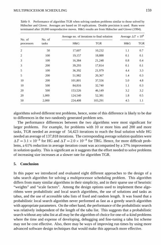
Hubscher and Glover (1994) give performance data for an algorithm solving 110 randomlygenerated problems similar to the ones solved here. Ten problems were generated and solvedfor eleven different combinations of processors and servers. Problem difficulty ranged fromrelatively easy (2 processors and 20 tasks) to somewhat difficult (50 processors and 2,000tasks). All task durations were drawn from a uniform distribution with a range from zeroto one. For each set of 10 problems the average number of iterations needed to reach thefinal solution was reported, as was the average range and average value of the performancemeasure1t . Their results and the corresponding values for algorithm TGR solving similarproblems are listed in Table 9.

It is seen that algorithm TGR in all but one case used fewer iterations to reach the finalsolution. In fact, algorithm TGR needed on the average 34,786 iterations to reach the finalsolution while, on the average 78,082 iterations were needed for algorithm HG. It shouldbe noted that the test problems solved by the two algorithms were different, although theywere generated in the same way. Hence, some of these differences are likely to be dueto differences in the two randomly generated problem sets. However, at-test confirmedon the 95% level, the hypothesis that the mean iteration counts were drawn from differentpopulations.

The data in Table 9 also shows that this improvement in efficiency is accompanied bya corresponding improvement in solution quality. The average value of1T for the solu-tions obtained by algorithm TGR was 1.4× 10−8 while it was 2.1× 10−8 for the solutionsobtained by algorithm HG. In no case did algorithm HG yield a solution with a higherquality than the one obtained by algorithm TGR. Again, it should be noted that the two

P1: SAD



Table 9. Performance of algorithm TGR when solving random problems similar to those solved byHubscher and Glover. Averages are based on 10 replications. Double precision is used. Runs wereterminated after 20,000 nonproductive moves. H&G results are from H¨ubscher and Glover (1994).

Average no. of iterations to final solution Average1T × 108

No. ofprocessors

No. oftasks H&G TGR H&G TGR

2 50 17,607 10,232 1.1 0.7

2 100 19,157 18,888 0.1 0.1

3 100 16,384 21,248 0.8 0.4

3 200 39,293 17,814 0.1 0.1

5 100 36,392 21,979 4.4 3.3

5 200 51,982 20,367 1.4 0.3

10 200 101,801 37,556 5.0 4.8

10 500 84,816 32,740 1.1 0.3

20 500 153,526 46,149 3.2 3.2

20 1,000 124,540 52,381 1.8 0.5

50 2,000 224,408 103,291 4.5 1.1

algorithms solved different test problems, hence, some of this difference is likely to be dueto differences in the two randomly generated problem sets.

The performance differences between the two algorithms were most significant forlarger problems. For example, for problems with 10 or more bins and 200 and moretasks, TGR needed an average of 54,423 iterations to reach the final solution while HGneeded an average of 137,818 iterations. The corresponding average solution qualities were1T = 3.1× 10−8 for HG and1T = 2.0× 10−8 for TRG. Hence, for more difficult prob-lems, a 61% reduction in average iteration count was accompanied by a 37% improvementin solution quality. This is significant as it suggests that the effort needed to solve problemsof increasing size increases at a slower rate for algorithm TGR.

5. Conclusion

In this paper we introduced and evaluated eight different approaches to the design of atabu search algorithm for solving a multiprocessor scheduling problem. This algorithmdiffers from many similar algorithms in their simplicity, and in their sparse use of heuristic“weights” and “scale factors”. Among the design options used to implement these algo-rithms were probabilistic and local search algorithms, the use of solutions and tasks astabus, and the use of accessible tabu lists of fixed and random length. It was found that aprobabilistic local search algorithm never performed as fast as a greedy search algorithmwith appropriate parameters. On the other hand, the performance of the probabilistic searchwas relatively independent of the length of the tabu list. This suggests that a probabilisticsearch without any tabu list at all may be the algorithm of choice for one-of-a-kind problemswhere the time and expense of developing, debugging and fine-tuning a tabu list schememay not be cost effective. Also, there may be ways of improving run times by using moreadvanced software design techniques that would make this approach more effective.

P1: SAD


160 THESEN

The use of accessible tabu lists of random length improved the performance of all algo-rithms. This improvement was particularly significant for algorithms using tasks as tabus.Hash coding without conflict resolution proved to be an effective way to manage solutionson the tabu list. The efficiency of this approach was evidenced by a barely noticeableincrease in solution times as the length of the list increased. Long tabu lists were effectivewhen solutions were used. Although hash-coded solutions were effective list entries, theuse of recently moved tasks proved to be even more effective when an accessible list ofrandom length was used. This increase in efficiency can at least in part be attributed to thefact that no list management was needed when tasks were used.

All algorithms were sensitive to the choice of the list length parameter. Too short alist resulted in exceptionally poor performance for algorithms using a greedy local search.Longer lists quickly degraded performance when tasks were tabus. Performance was de-graded much more slowly when solutions were used. In all cases, it would be better touse a list length longer than the optimal one than one shorter than the optimal one. Largeand complex problems were more sensitive to the choice of list length than were smaller,simpler problems.

References

Anderson, Charles A., Kathryn Fraughnaugh, Mark Parker, and Jennifer Ryan. (1993). “Path Assignment for CallRouting: An Application of Tabu Search,”Annals of Operations Research41, 301–312.

Barnes, J.W. and M. Laguna. (1993). “A Tabu Search Experience in Production Scheduling,”Annals of OperationsResearch41, 141–156.

Barnes, J.W., M. Laguna, and F. Glover. (1995). “An Overview of Tabu Search Approaches to Production Schedul-ing Problems.” In D.E. Brown and W.T. Scherer (eds.),Intelligent Scheduling System. Kluwer Academic Pub-lishers, pp. 101–127.

Blazewicz, J., K.E. Ecker E. Pesch, G. Schmidt, and J. Weglarz. (1995).Scheduling Computer and ManufacturingProcesses. Berlin: Springer-Verlag.

Glover, F. (1986). “Future Paths for Integer Programming and Links to Artificial Intelligence,”Computers andOperations Research13, 533–549.

Glover, F. (1995). “Tabu Search Fundamentals and Uses, Revised and Expanded: April 1995.” Technical Report,Graduate School of Business, University of Colorado, Bolder, CO.

Glover, F. and M. Laguna. (1997).Tabu Search. Boston: Kluwer Academic Publishers.Graham, R.L. (1969). “Bounds for Certain Multiprocessing Anomalities,”SIAM J. Appl. Math. 17, 263–269.Graham, R.L. (1976). “Bounds on Performance of Scheduling Algorithms.” In E.G. Coffman, Jr. (ed.),Scheduling

in Computer and Job Shop Systems. Chapt. 5, New York: John Wiley.Johnson, D.S., A Demers, J.D. Ullman, M.R. Garey, and R.L. Graham. (1974). “Worst Case Performance Bounds

for Simple One-Dimensional Packing Algorithms,”SIAM Journal on Computing3, 299–326.Hubscher, Roland and F. Glover. (1994). “Applying Tabu Search with Influential Diversification to Multiprocessor

Scheduling,”Computers in Operations Research21, 877–844.Kampke, Thomas. (1988). “Simulated Annealing: Use of a New Tool in Bin Packing,”Annals of Operations

Research16, 327–332.Knuth, D. (1973).The Art of Computer Programming: Sorting and Searching. Reading, MA: Addison-Wesley.Laguna, M. and F. Glover. (1993). “Integrating Target Analysis and Tabu Search for Improved Scheduling Systems,”

Expert Systems With Applications6, 287–297.Løkketangen, A. (1995). “Tabu Search as a Metaheuristic Guide for Combinatorial Optimization Problems,” Dr.

Scient. Thesis, Institute for Informatics, University of Bergen, Bergen, Norway.Morton, T.E. and David W. Pentico. (1993).Heuristic Scheduling Systems. New York, NY: John Wiley & Sons.Osman, I. and J.P. Kelly (eds.). (1996).Meta-Heuristics. Theory and Applications. Boston: Kluwer Academic

Publishers.Taillard, Eric D. (1994). “Parallel Taboo Search Techniques for the Job Shop Scheduling Problem,”ORSA Journal

on Computing6(2), 108–117.

design and evaluation of tabu search algorithms for multiprocessor scheduling

Documents