descriptive statistics-i - judoctors · in this lecture we discuss using descriptive statistics, as...
TRANSCRIPT
Descriptive Statistics-I
Dr Mahmoud Alhussami
Biostatistics
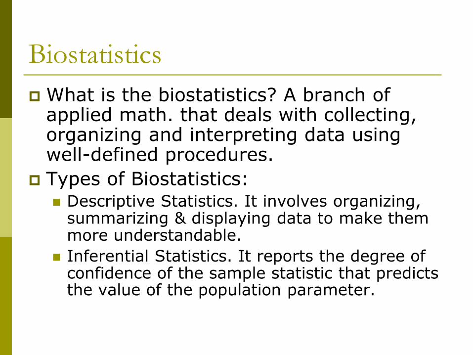
What is the biostatistics? A branch of applied math. that deals with collecting, organizing and interpreting data using well-defined procedures.
Types of Biostatistics: Descriptive Statistics. It involves organizing,
summarizing & displaying data to make them more understandable.
Inferential Statistics. It reports the degree of confidence of the sample statistic that predicts the value of the population parameter.
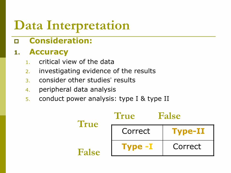
Data Interpretation Consideration:
1. Accuracy
1. critical view of the data
2. investigating evidence of the results
3. consider other studies’ results
4. peripheral data analysis
5. conduct power analysis: type I & type II
Correct Type-II
Type -I Correct
True
False
True False
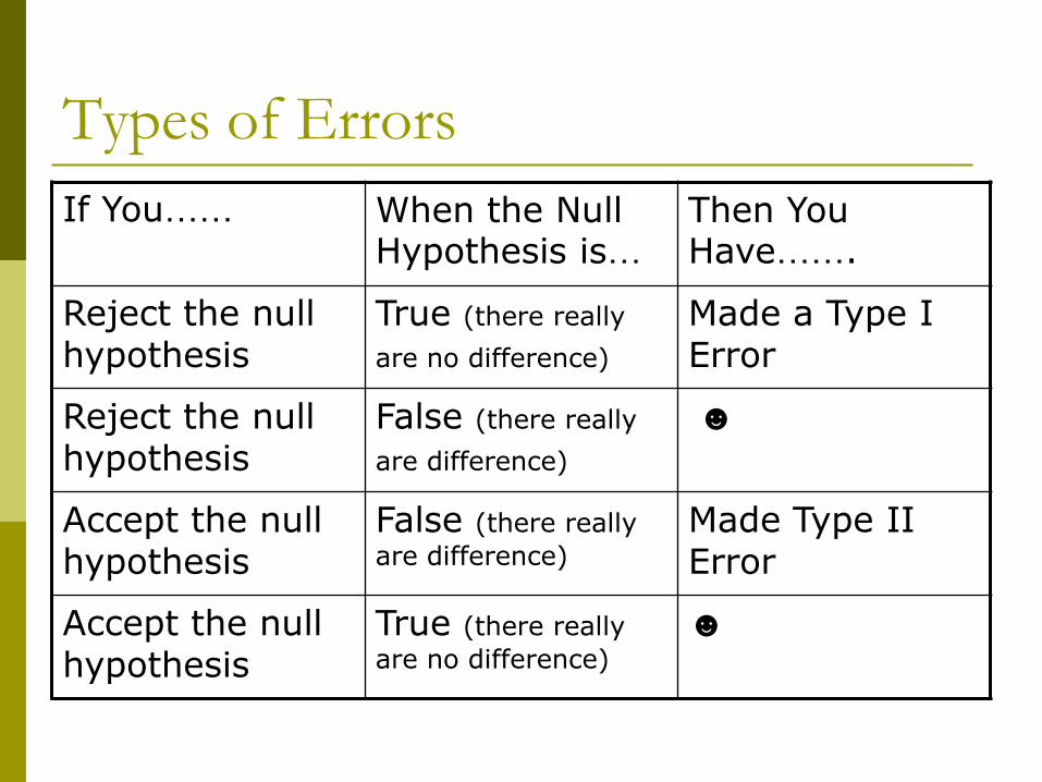
Types of Errors
If You…… When the Null Hypothesis is…
Then You Have…….
Reject the null hypothesis
True (there really
are no difference)
Made a Type I Error
Reject the null hypothesis
False (there really
are difference)
☻
Accept the null hypothesis
False (there really
are difference)
Made Type II Error
Accept the null hypothesis
True (there really
are no difference)
☻
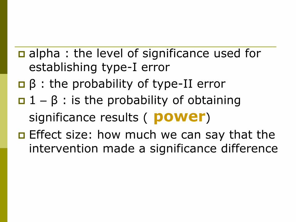
alpha : the level of significance used for establishing type-I error
β : the probability of type-II error
1 – β : is the probability of obtaining
significance results ( power)
Effect size: how much we can say that the intervention made a significance difference
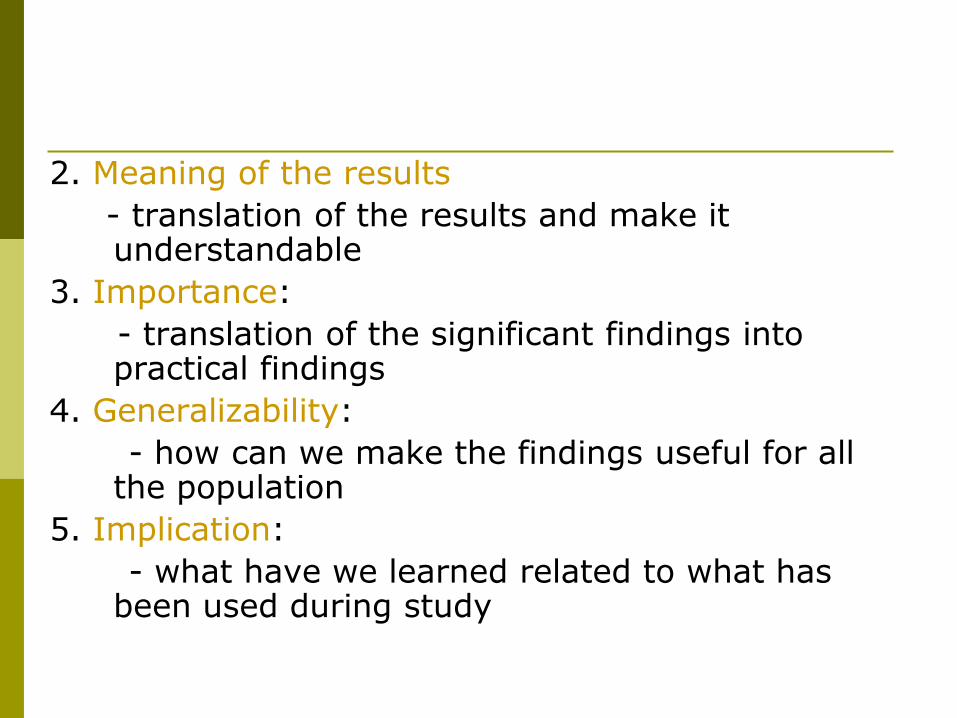
2. Meaning of the results
- translation of the results and make it understandable
3. Importance:
- translation of the significant findings into practical findings
4. Generalizability:
- how can we make the findings useful for all the population
5. Implication:
- what have we learned related to what has been used during study
25 February 2014 7
Definition
Data is any type of information
Raw data is a data collected as they receive.
Organize data is data organized either in ascending, descending or in a grouped data.
25 February 2014 8
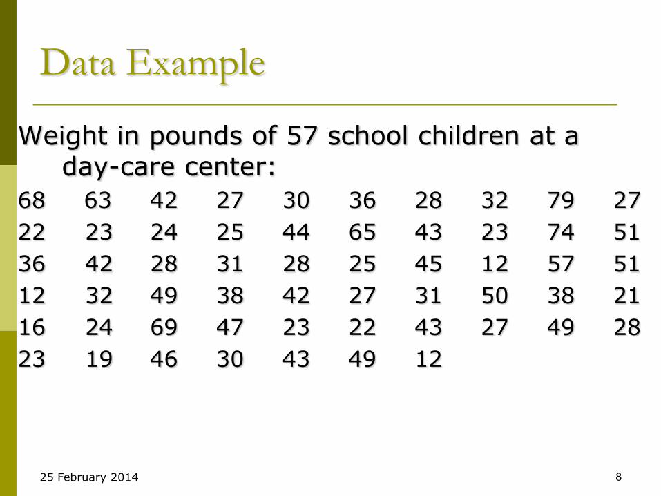
Data Example
Weight in pounds of 57 school children at a day-care center:
68 63 42 27 30 36 28 32 79 27
22 23 24 25 44 65 43 23 74 51
36 42 28 31 28 25 45 12 57 51
12 32 49 38 42 27 31 50 38 21
16 24 69 47 23 22 43 27 49 28
23 19 46 30 43 49 12
Descriptive Statistics
In this lecture we discuss using descriptive statistics, as opposed to inferential statistics.
Here we are interested only in summarizing the data in front of us, without assuming that it represents anything more.
We will look at both numerical and categorical data.
We will look at both quantitative and graphical techniques.
The basic overall idea is to turn data into information.
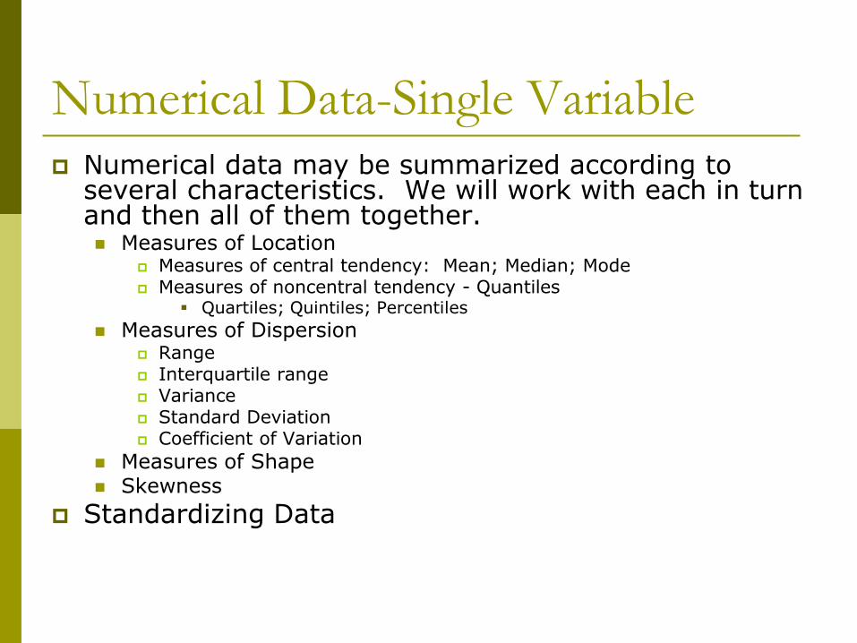
Numerical Data-Single Variable
Numerical data may be summarized according to several characteristics. We will work with each in turn and then all of them together. Measures of Location
Measures of central tendency: Mean; Median; Mode Measures of noncentral tendency - Quantiles
Quartiles; Quintiles; Percentiles
Measures of Dispersion Range Interquartile range Variance Standard Deviation Coefficient of Variation
Measures of Shape Skewness
Standardizing Data
Measures of Location
Measures of location place the data set on the scale of real numbers.
It refers to the location of a typical data value-the data value around which other scores to cluster.
Measures of central tendency (i.e., central location) help find the approximate center of the dataset.
Researchers usually do not use the term average, because there are three alternative types of average.
These include the mean, the median, and the mode. In a perfect world, the mean, median & mode would be the same.
However, the world is not perfect & very often, the mean, median and mode are not the same
25 February 2014 12
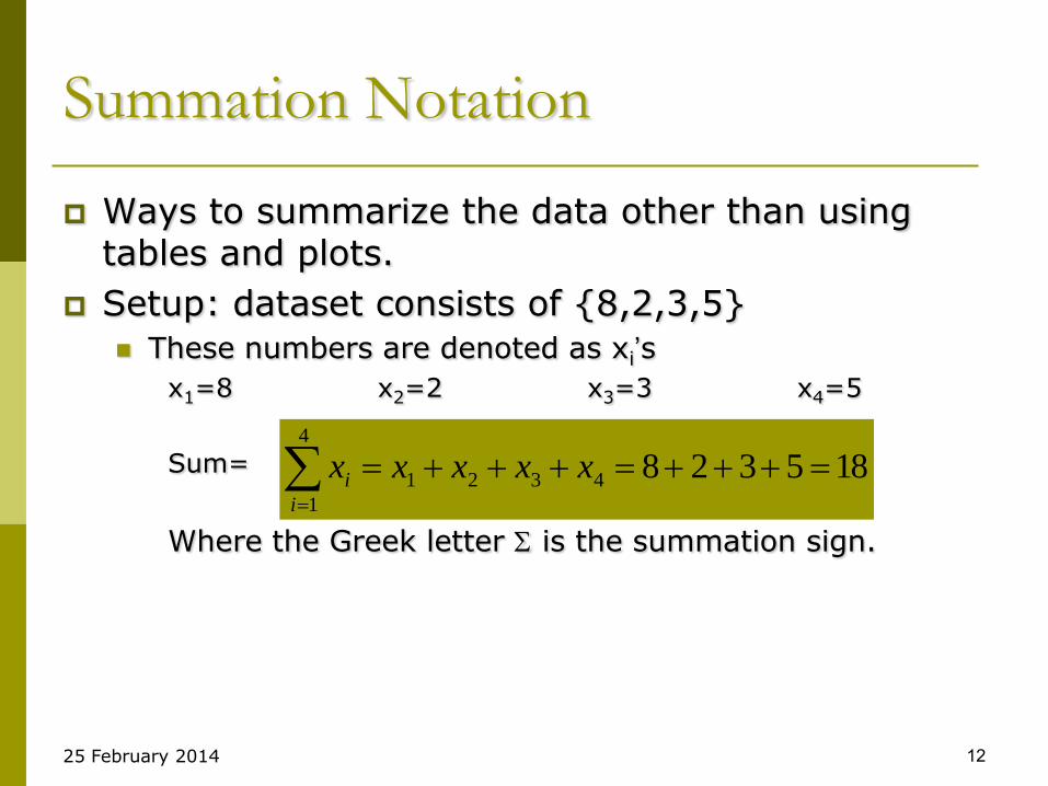
Summation Notation
Ways to summarize the data other than using tables and plots.
Setup: dataset consists of {8,2,3,5}
These numbers are denoted as xi’s
x1=8 x2=2 x3=3 x4=5
Sum=
Where the Greek letter is the summation sign.
4
1
4321 185328i
i xxxxx
13
25 February 2014 14
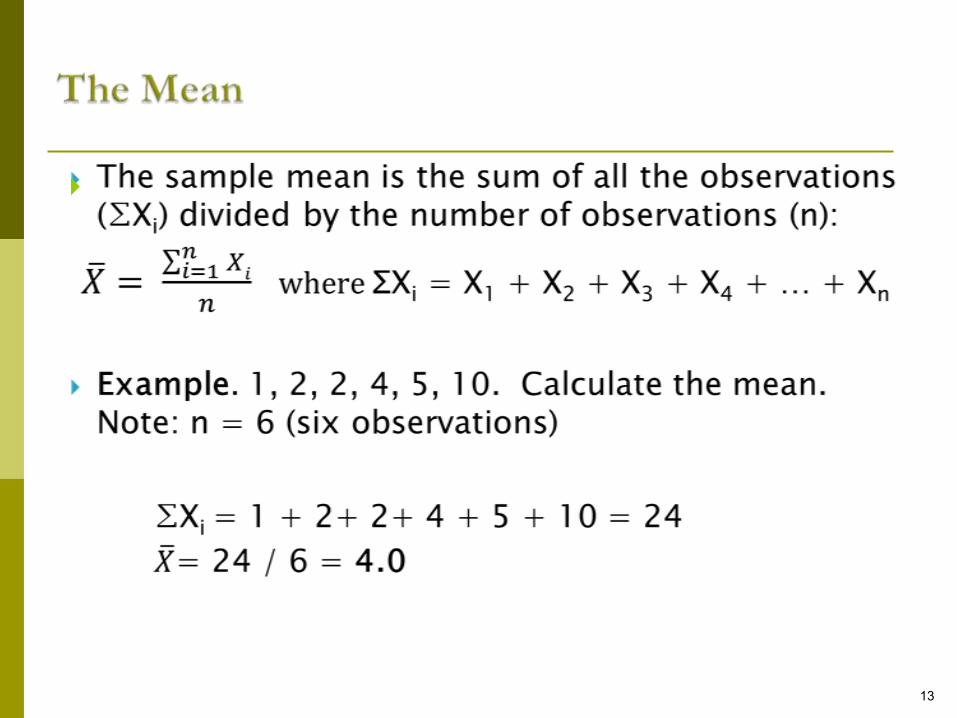
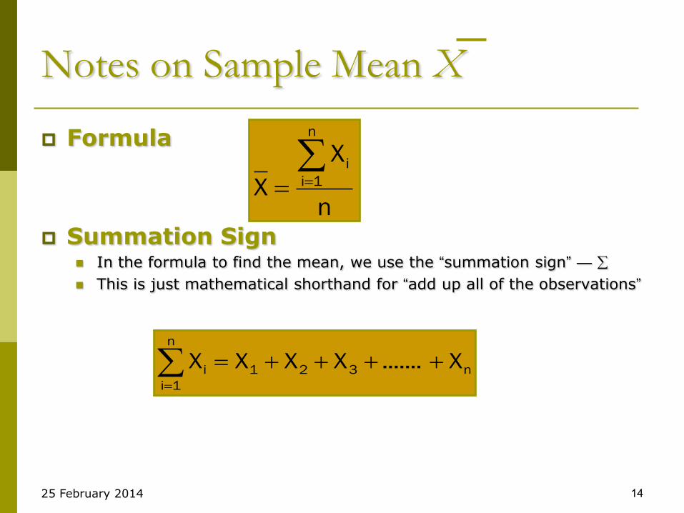
Notes on Sample Mean X
Formula
Summation Sign In the formula to find the mean, we use the ―summation sign‖ —
This is just mathematical shorthand for ―add up all of the observations‖
n
X
X
n
1i
i
n321
n
1i
i X.......XXXX
25 February 2014 15
Notes on Sample Mean
Also called sample average or arithmetic mean
Mean for the sample = X or M, Mean for
population = mew (μ)
Sensitive to extreme values
One data point could make a great change in sample mean
Why is it called the sample mean?
To distinguish it from population mean
16
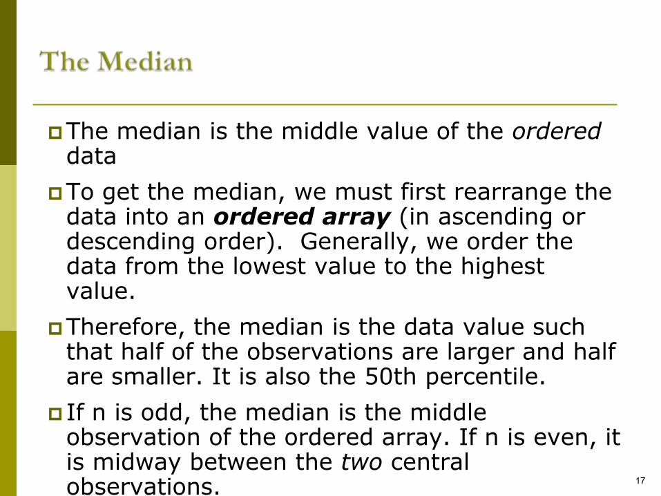
The median is the middle value of the ordereddata
To get the median, we must first rearrange the data into an ordered array (in ascending or descending order). Generally, we order the data from the lowest value to the highest value.
Therefore, the median is the data value such that half of the observations are larger and half are smaller. It is also the 50th percentile.
If n is odd, the median is the middle observation of the ordered array. If n is even, it is midway between the two central observations. 17
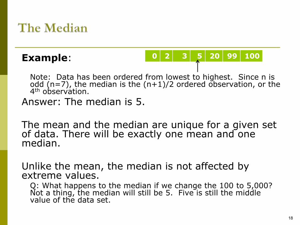
Example:
Note: Data has been ordered from lowest to highest. Since n is odd (n=7), the median is the (n+1)/2 ordered observation, or the 4th observation.
Answer: The median is 5.
The mean and the median are unique for a given set of data. There will be exactly one mean and one median.
Unlike the mean, the median is not affected by extreme values.
Q: What happens to the median if we change the 100 to 5,000? Not a thing, the median will still be 5. Five is still the middle value of the data set.
18
0 2 3 5 20 99 100
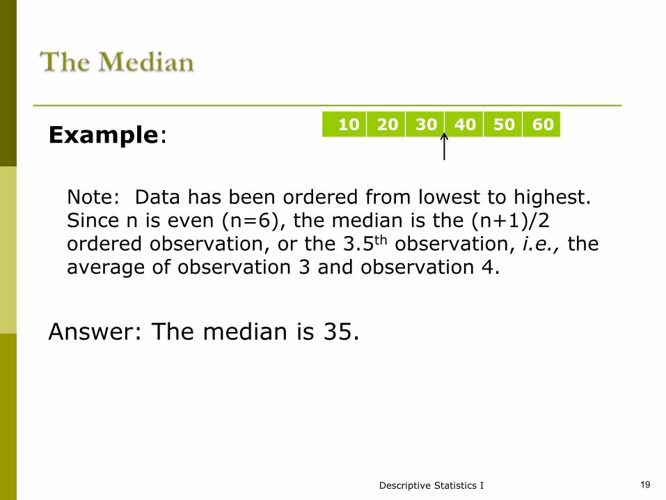
Example:
Note: Data has been ordered from lowest to highest. Since n is even (n=6), the median is the (n+1)/2 ordered observation, or the 3.5th observation, i.e., the average of observation 3 and observation 4.
Answer: The median is 35.
Descriptive Statistics I 19
10 20 30 40 50 60
20
25 February 2014 21
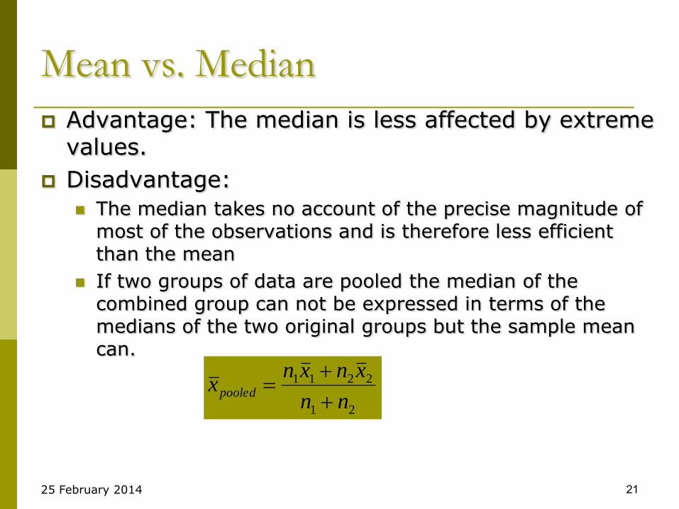
Mean vs. Median
Advantage: The median is less affected by extreme values.
Disadvantage:
The median takes no account of the precise magnitude of most of the observations and is therefore less efficient than the mean
If two groups of data are pooled the median of the combined group can not be expressed in terms of the medians of the two original groups but the sample mean can.
21
2211
nn
xnxnxpooled
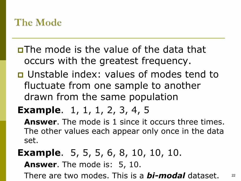
The mode is the value of the data that occurs with the greatest frequency.
Unstable index: values of modes tend to fluctuate from one sample to another drawn from the same population
Example. 1, 1, 1, 2, 3, 4, 5
Answer. The mode is 1 since it occurs three times. The other values each appear only once in the data set.
Example. 5, 5, 5, 6, 8, 10, 10, 10.
Answer. The mode is: 5, 10.
There are two modes. This is a bi-modal dataset. 22
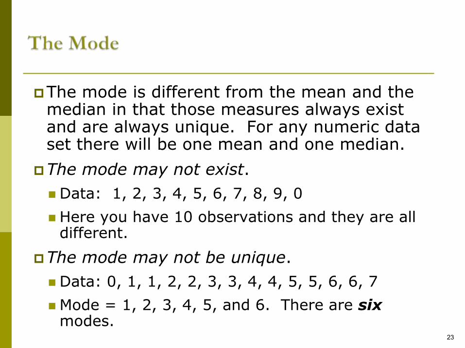
The mode is different from the mean and the median in that those measures always exist and are always unique. For any numeric data set there will be one mean and one median.
The mode may not exist.
Data: 1, 2, 3, 4, 5, 6, 7, 8, 9, 0
Here you have 10 observations and they are all different.
The mode may not be unique.
Data: 0, 1, 1, 2, 2, 3, 3, 4, 4, 5, 5, 6, 6, 7
Mode = 1, 2, 3, 4, 5, and 6. There are sixmodes.
23
Comparison of the Mode, the Median,
and the Mean
In a normal distribution, the mode , the median, and the mean have the same value.
The mean is the widely reported index of central tendency for variables measured on an interval and ratio scale.
The mean takes each and every score into account.
It also the most stable index of central tendency and thus yields the most reliable estimate of the central tendency of the population.
Comparison of the Mode, the Median,
and the Mean
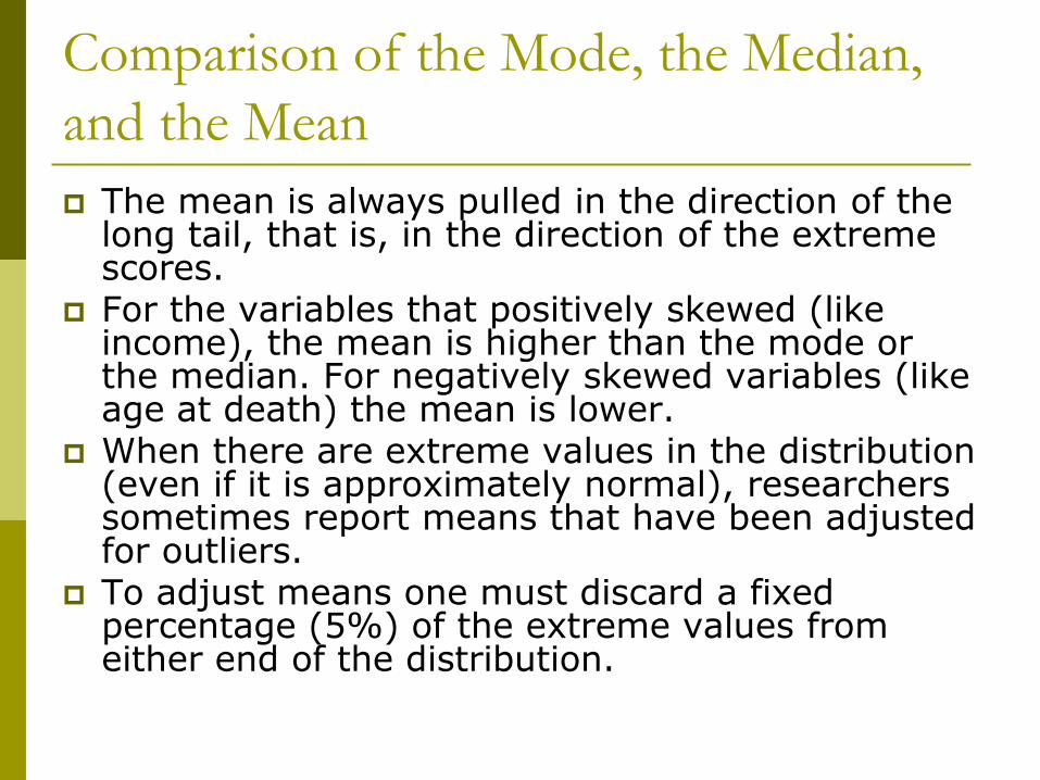
The mean is always pulled in the direction of the long tail, that is, in the direction of the extreme scores.
For the variables that positively skewed (like income), the mean is higher than the mode or the median. For negatively skewed variables (like age at death) the mean is lower.
When there are extreme values in the distribution (even if it is approximately normal), researchers sometimes report means that have been adjusted for outliers.
To adjust means one must discard a fixed percentage (5%) of the extreme values from either end of the distribution.
25 February 2014 26
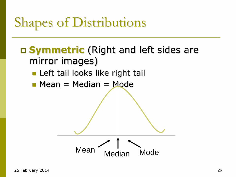
Shapes of Distributions
Symmetric (Right and left sides are mirror images)
Left tail looks like right tail
Mean = Median = Mode
MeanMedian Mode
25 February 2014 27
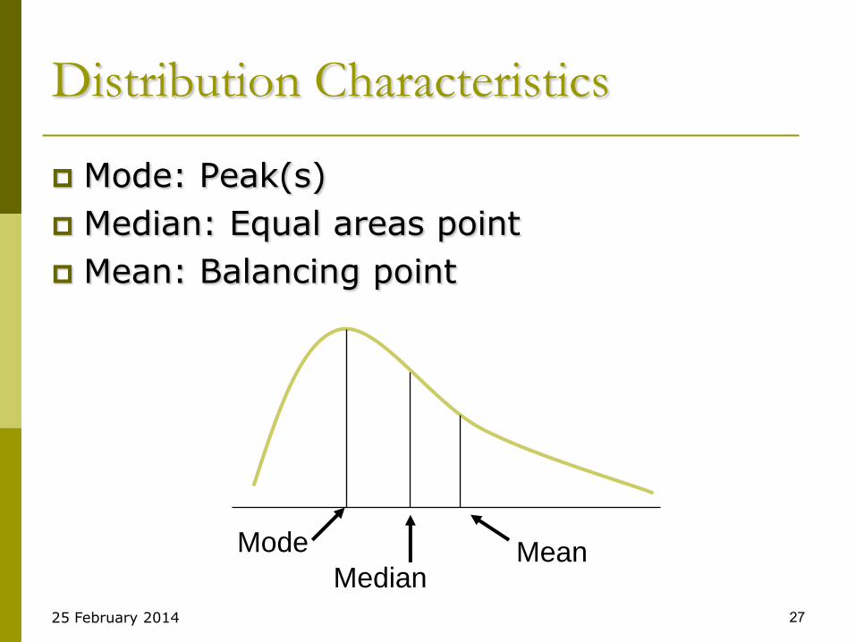
Distribution Characteristics
Mode: Peak(s)
Median: Equal areas point
Mean: Balancing point
MeanMode
Median
25 February 2014 28
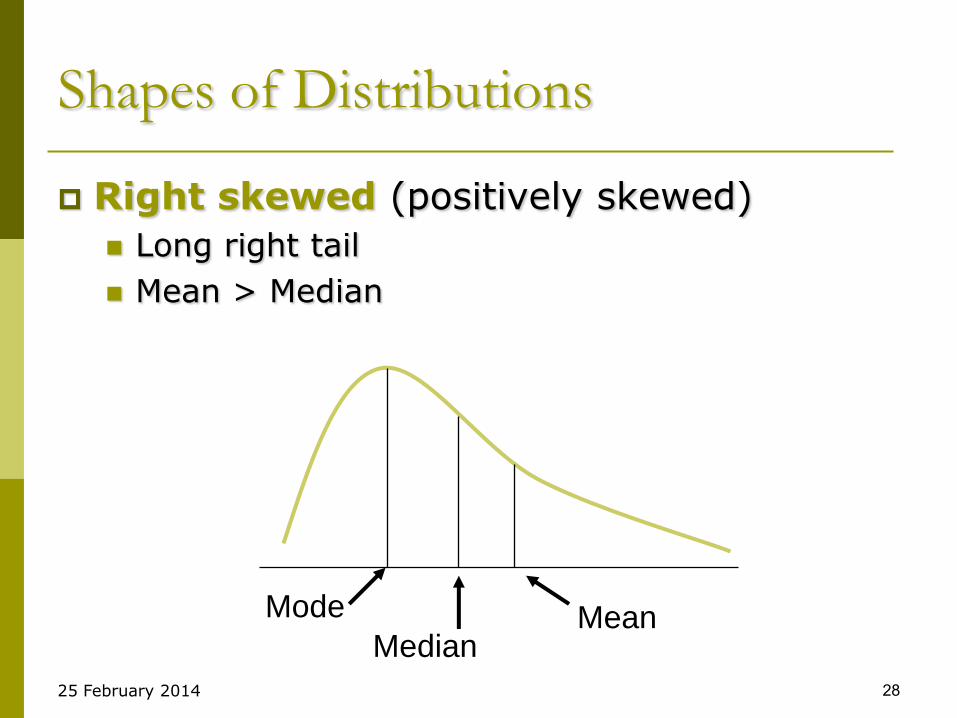
Shapes of Distributions
Right skewed (positively skewed)
Long right tail
Mean > Median
MeanMode
Median
25 February 2014 29
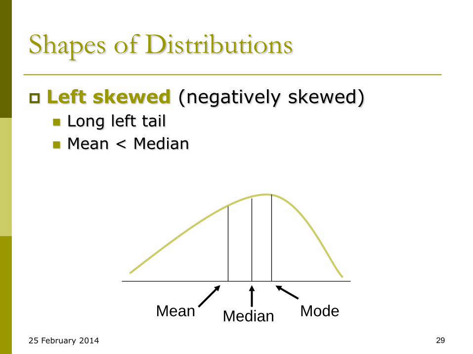
Shapes of Distributions
Left skewed (negatively skewed)
Long left tail
Mean < Median
ModeMedianMean
25 February 2014 30
SPSS Functions
If you are given the ―raw data‖ (i.e. data
not summarized in a frequency table) you can calculate the measures of location in SPSS.
Descriptive Command
Option Command
Selection of mean, median and mode
Measures of non-central location used to summarize a set of data
Examples of commonly used quantiles:
Quartiles
Quintiles
Deciles
Percentiles
Descriptive Statistics I 31
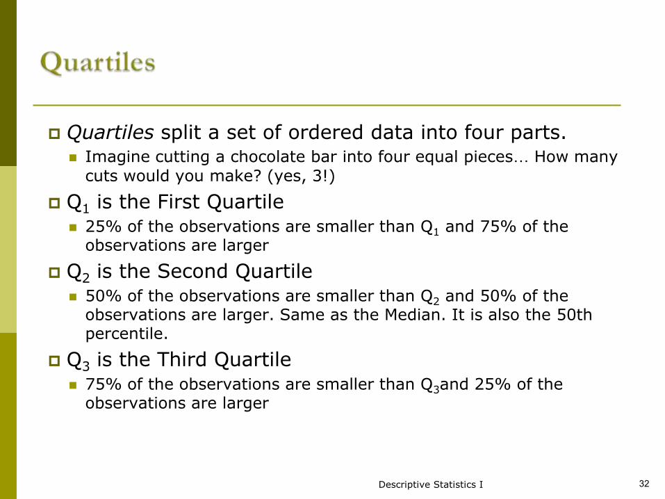
Quartiles split a set of ordered data into four parts. Imagine cutting a chocolate bar into four equal pieces… How many
cuts would you make? (yes, 3!)
Q1 is the First Quartile 25% of the observations are smaller than Q1 and 75% of the
observations are larger
Q2 is the Second Quartile 50% of the observations are smaller than Q2 and 50% of the
observations are larger. Same as the Median. It is also the 50th percentile.
Q3 is the Third Quartile 75% of the observations are smaller than Q3and 25% of the
observations are larger
Descriptive Statistics I 32
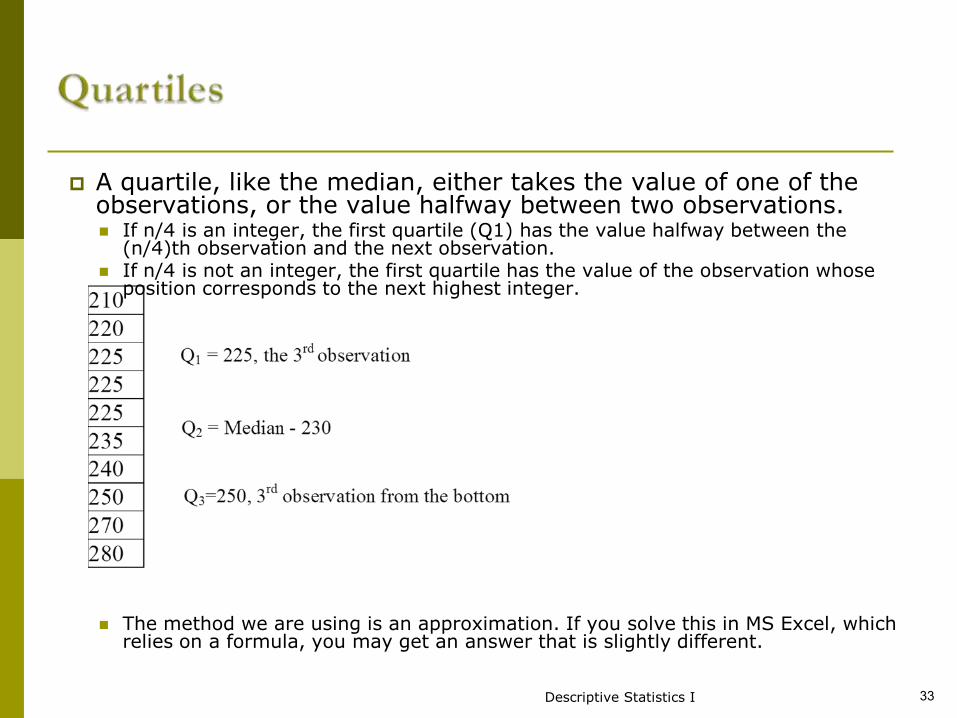
A quartile, like the median, either takes the value of one of the observations, or the value halfway between two observations. If n/4 is an integer, the first quartile (Q1) has the value halfway between the
(n/4)th observation and the next observation. If n/4 is not an integer, the first quartile has the value of the observation whose
position corresponds to the next highest integer.
The method we are using is an approximation. If you solve this in MS Excel, which relies on a formula, you may get an answer that is slightly different.
Descriptive Statistics I 33
34
Similar to what we just learned about quartiles, where 3 quartiles split the data into 4 equal parts,
There are 9 deciles dividing the distribution into 10 equal portions (tenths).
There are four quintiles dividing the population into 5 equal portions.
… and 99 percentiles (next slide)
In all these cases, the convention is the same. The point, be it a quartile, decile, or percentile, takes the value of one of the observations or it has a value halfway between two adjacent observations. It is never necessary to split the difference between two observations more finely.
Descriptive Statistics I 35
We use 99 percentiles to divide a data set into 100 equal portions.
Percentiles are used in analyzing the results of standardized exams. For instance, a score of 40 on a standardized test might seem like a terrible grade, but if it is the 99th percentile, don’t worry about telling your parents. ☺
Which percentile is Q1? Q2 (the median)? Q3?
We will always use computer software to obtain the percentiles.
36
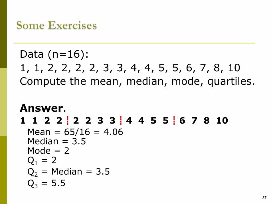
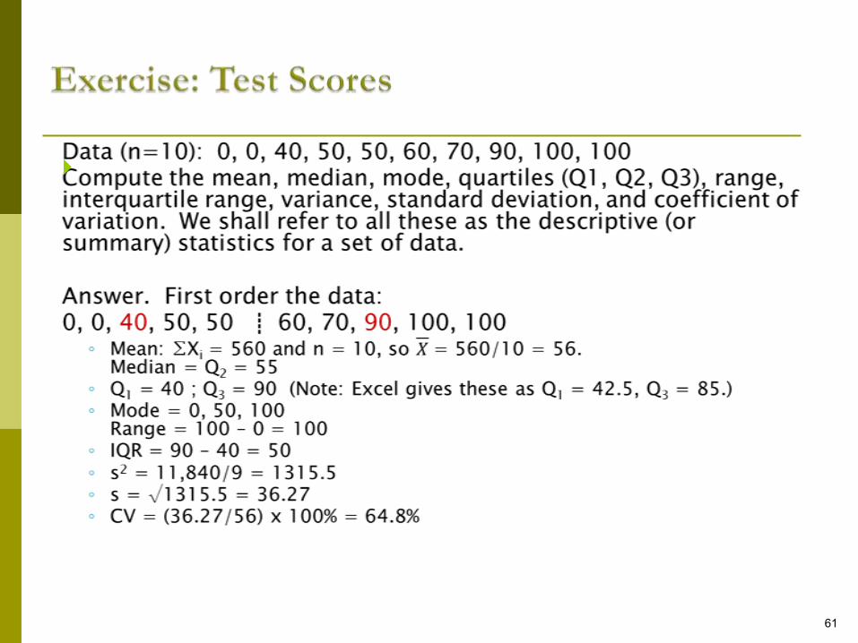
Data (n=16):
1, 1, 2, 2, 2, 2, 3, 3, 4, 4, 5, 5, 6, 7, 8, 10
Compute the mean, median, mode, quartiles.
Answer.1 1 2 2 ┋ 2 2 3 3 ┋ 4 4 5 5 ┋ 6 7 8 10
Mean = 65/16 = 4.06Median = 3.5Mode = 2Q1 = 2
Q2 = Median = 3.5
Q3 = 5.5
37
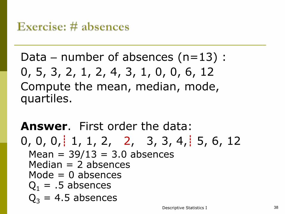
Data – number of absences (n=13) :
0, 5, 3, 2, 1, 2, 4, 3, 1, 0, 0, 6, 12
Compute the mean, median, mode, quartiles.
Answer. First order the data:
0, 0, 0,┋ 1, 1, 2, 2, 3, 3, 4,┋ 5, 6, 12Mean = 39/13 = 3.0 absencesMedian = 2 absencesMode = 0 absencesQ1 = .5 absences
Q3 = 4.5 absencesDescriptive Statistics I 38
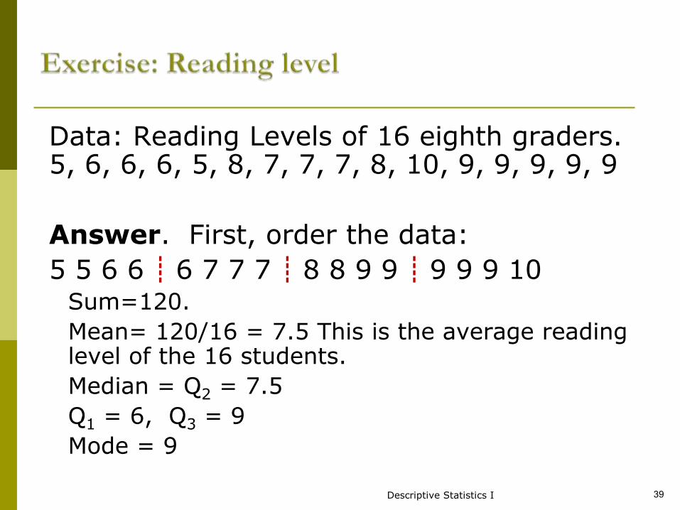
Data: Reading Levels of 16 eighth graders.5, 6, 6, 6, 5, 8, 7, 7, 7, 8, 10, 9, 9, 9, 9, 9
Answer. First, order the data:
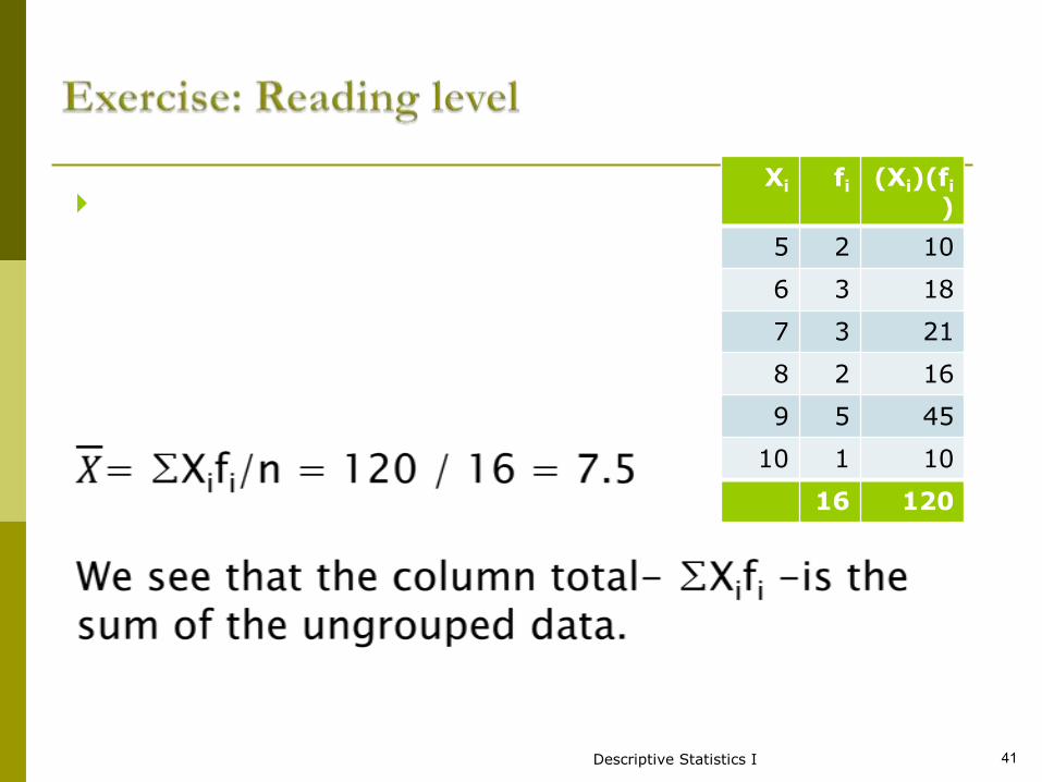
5 5 6 6 ┋ 6 7 7 7 ┋ 8 8 9 9 ┋ 9 9 9 10Sum=120.
Mean= 120/16 = 7.5 This is the average reading level of the 16 students.
Median = Q2 = 7.5
Q1 = 6, Q3 = 9
Mode = 9
Descriptive Statistics I 39
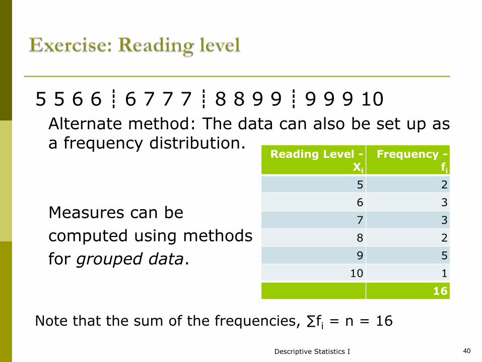
5 5 6 6 ┋ 6 7 7 7 ┋ 8 8 9 9 ┋ 9 9 9 10
Alternate method: The data can also be set up as a frequency distribution.
Measures can be
computed using methods
for grouped data.
Note that the sum of the frequencies, ∑fi = n = 16
Descriptive Statistics I 40
Reading Level -Xi
Frequency -fi
5 2
6 3
7 3
8 2
9 5
10 1
16
Descriptive Statistics I 41
Xi fi (Xi)(fi
)
5 2 10
6 3 18
7 3 21
8 2 16
9 5 45
10 1 10
16 120
It refers to how spread out the scores are.In other words, how similar or different
participants are from one another on the variable. It is either homogeneous or heterogeneous sample.
Why do we need to look at measures of dispersion?
Consider this example:A company is about to buy computer chips that must have an average life of 10 years. The company has a choice of two suppliers. Whose chips should they buy? They take a sample of 10 chips from each of the suppliers and test them. See the data on the next slide.
42
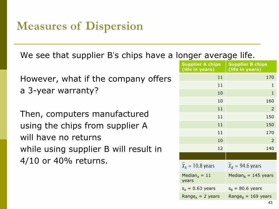
We see that supplier B’s chips have a longer average life.
However, what if the company offers
a 3-year warranty?
Then, computers manufactured
using the chips from supplier A
will have no returns
while using supplier B will result in
4/10 or 40% returns.
43
Supplier A chips (life in years)
Supplier B chips (life in years)
11 170
11 1
10 1
10 160
11 2
11 150
11 150
11 170
10 2
12 140
MedianA = 11 years
MedianB = 145 years
sA = 0.63 years sB = 80.6 years
RangeA = 2 years RangeB = 169 years
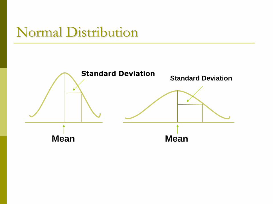
Normal Distribution
Mean
Standard DeviationStandard Deviation
Mean
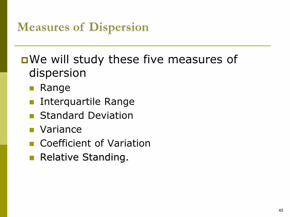
We will study these five measures of dispersion
Range
Interquartile Range
Standard Deviation
Variance
Coefficient of Variation
Relative Standing.
45
The Range
Is the simplest measure of variability, is the difference between the highest score and the lowest score in the distribution.
In research, the range is often shown as the minimum and maximum value, without the abstracted difference score.
It provides a quick summary of a distribution’s
variability.
It also provides useful information about a distribution when there are extreme values.
The range has two values, it is highly unstable.
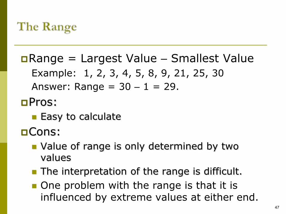
Range = Largest Value – Smallest Value
Example: 1, 2, 3, 4, 5, 8, 9, 21, 25, 30
Answer: Range = 30 – 1 = 29.
Pros:
Easy to calculate
Cons:
Value of range is only determined by two values
The interpretation of the range is difficult.
One problem with the range is that it is influenced by extreme values at either end.
47
48
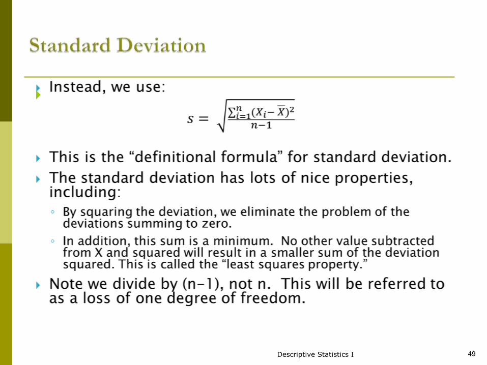
Descriptive Statistics I 49
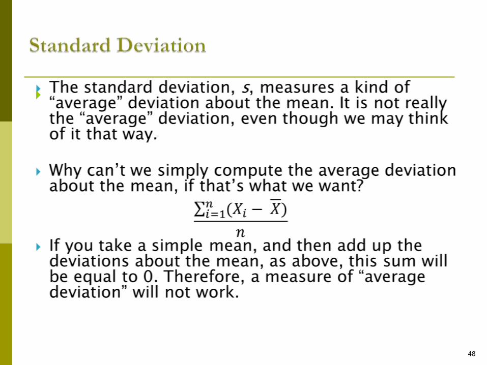
Standard Deviation
The smaller the standard deviation, the better is the mean as the summary of a typical score. E.g. 10 people weighted 150 pounds, the SD would be zero, and the mean of 150 would communicate perfectly accurate information about all the participants wt. Another example would be a heterogeneous sample 5 people 100 pounds and another five people 200 pounds. The mean still 150, but the SD would be 52.7.
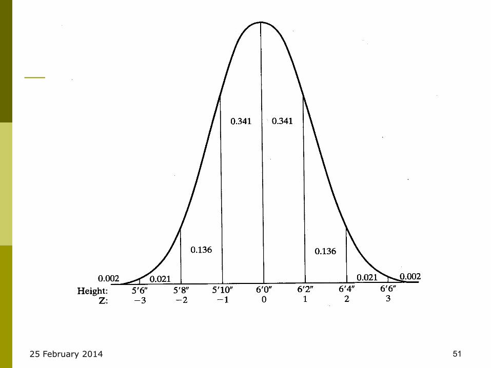
In normal distribution there are 3 SDs above the mean and 3 SDs below the mean.
25 February 2014 51
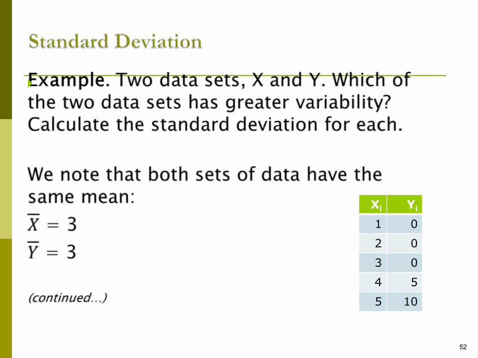
52
Xi Yi
1 0
2 0
3 0
4 5
5 10
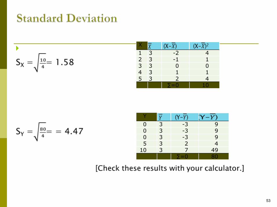
53
X
1 3 -2 42 3 -1 13 3 0 04 3 1 15 3 2 4
∑=0 10
Y
0 3 -3 90 3 -3 90 3 -3 95 3 2 4
10 3 7 49∑=0 80
54
55
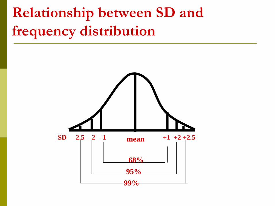
Relationship between SD and
frequency distribution
SD -2.5 -2 -1 +1 +2 +2.5mean
68%
95%
99%
25 February 2014 57
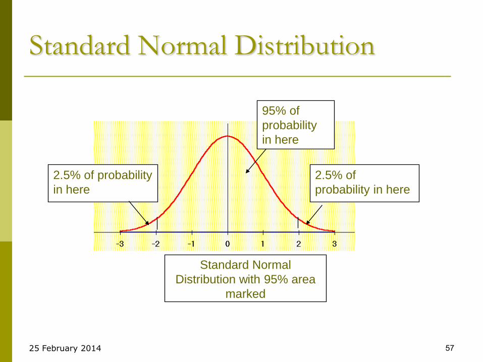
Standard Normal Distribution
2.5% of
probability in here
2.5% of probability
in here
95% of
probability
in here
Standard Normal
Distribution with 95% area
marked
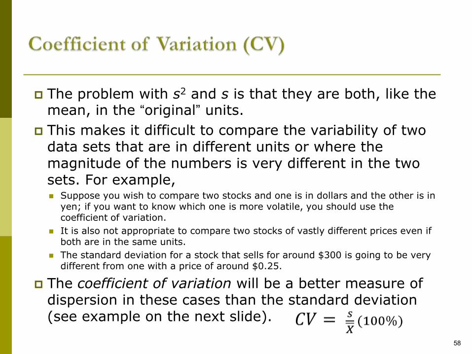
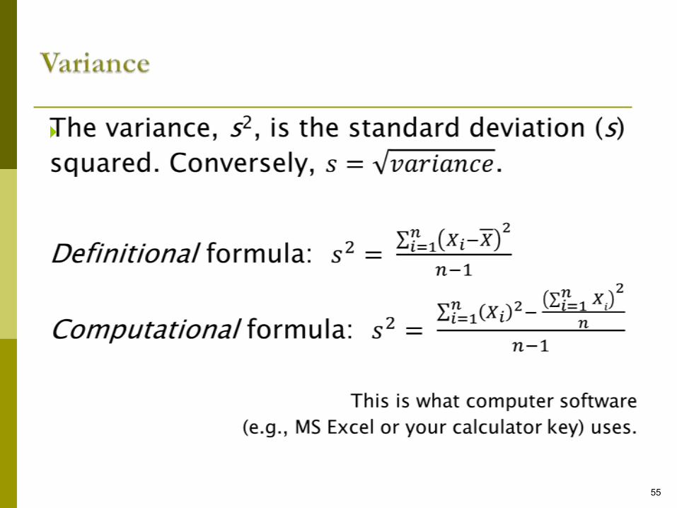
The problem with s2 and s is that they are both, like the mean, in the ―original‖ units.
This makes it difficult to compare the variability of two data sets that are in different units or where the magnitude of the numbers is very different in the two sets. For example, Suppose you wish to compare two stocks and one is in dollars and the other is in
yen; if you want to know which one is more volatile, you should use the coefficient of variation.
It is also not appropriate to compare two stocks of vastly different prices even if both are in the same units.
The standard deviation for a stock that sells for around $300 is going to be very different from one with a price of around $0.25.
The coefficient of variation will be a better measure of dispersion in these cases than the standard deviation (see example on the next slide).
58
Descriptive Statistics I 59
Descriptive Statistics I 60
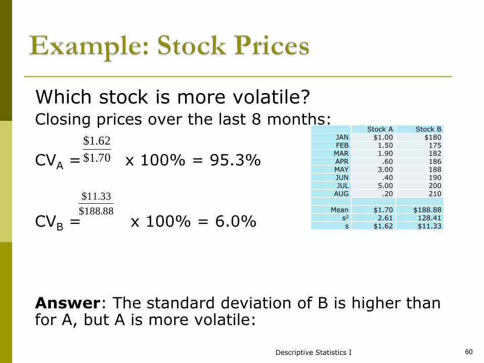
Which stock is more volatile?Closing prices over the last 8 months:
CVA = x 100% = 95.3%
CVB = x 100% = 6.0%
Answer: The standard deviation of B is higher than for A, but A is more volatile:
Stock A Stock BJAN $1.00 $180FEB 1.50 175MAR 1.90 182APR .60 186MAY 3.00 188JUN .40 190JUL 5.00 200
AUG .20 210
Mean $1.70 $188.88s2 2.61 128.41s $1.62 $11.33
70.1$
62.1$
88.188$
33.11$
61

Relative Standing
It provides information about the position of an individual score value within a distribution scores.
Two types:
Percentile Ranks.
Standard Scores.
Percentile Ranks It is the percentage of scores in the distribution that fall at
or below a given value. A percentile is a score value above which and below which
a certain percentage of value in a distribution fall. P = Number of scores less than a given score divided by
total number scores X 100.E.g. suppose you received a score of 90 on a test given to a class of 50 people. Of your classmates, 40 had scores lower than 90. P = 40/50 X 100 = 80. YOU achieved a higher score than 80% of the people who took the test, which also means that almost 20% who took the test did better than you.
Percentiles are symbolized by the letter P, with a subscript indicating the percentage below the score value. Hence, P60 refers to the 60th percentile and stands for the score below which 60% of values fall.
Percentile Ranks
The statement P40= 55 means that 40% of the values in the distribution fall below the score 55.
The are several interpercentile measures of variability. The most common being the Interquartile range (IQR).
IQR
The Interquartile range (IQR) is the score at the 75th percentile or 3rd quartile (Q3) minus the score at the 25th percentile or first quartile (Q1). Are the most used to define outliers.
It is not sensitive to extreme values.
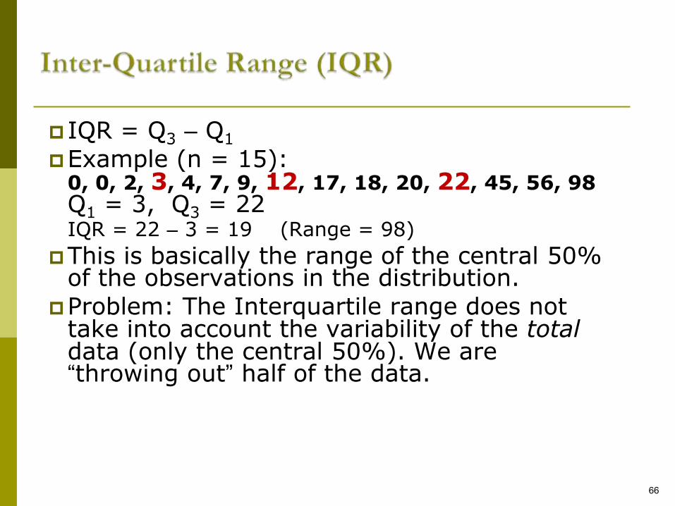
IQR = Q3 – Q1
Example (n = 15):0, 0, 2, 3, 4, 7, 9, 12, 17, 18, 20, 22, 45, 56, 98Q1 = 3, Q3 = 22IQR = 22 – 3 = 19 (Range = 98)
This is basically the range of the central 50% of the observations in the distribution.
Problem: The Interquartile range does not take into account the variability of the total data (only the central 50%). We are ―throwing out‖ half of the data.
66
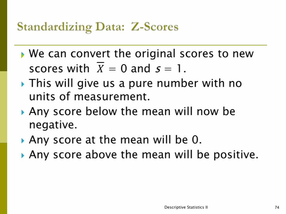
Standard Scores
There are scores that are expressed in terms of their relative distance from the mean. It provides information not only about rank but also distance between scores.
It often called Z-score.
Z Score
Is a standard score that indicates how many SDs from the mean a particular values lies.
Z = Score of value – mean of scores
divided by standard deviation.
25 February 2014 69
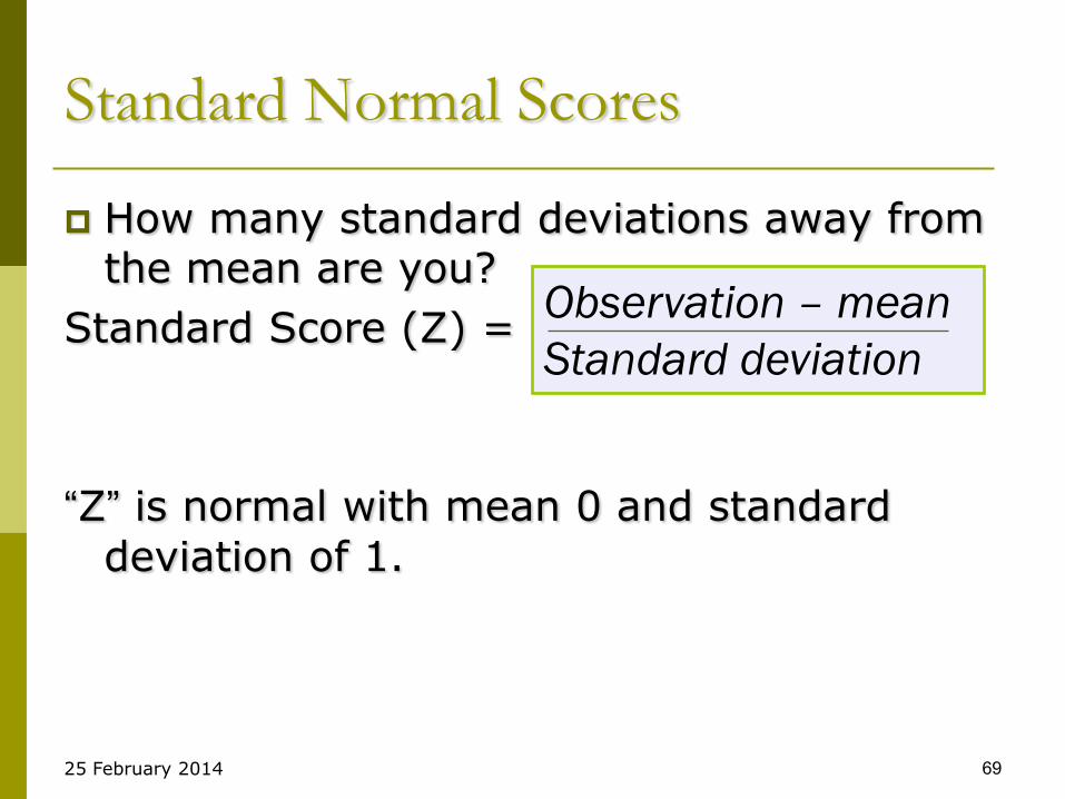
Standard Normal Scores
How many standard deviations away from the mean are you?
Standard Score (Z) =
―Z‖ is normal with mean 0 and standard
deviation of 1.
Observation – mean
Standard deviation

25 February 2014 70
25 February 2014 71
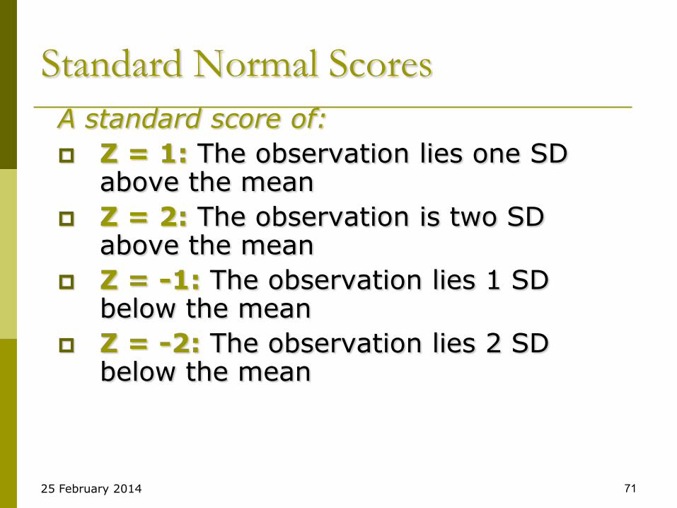
Standard Normal Scores
A standard score of:
Z = 1: The observation lies one SD above the mean
Z = 2: The observation is two SD above the mean
Z = -1: The observation lies 1 SD below the mean
Z = -2: The observation lies 2 SD below the mean
25 February 2014 72
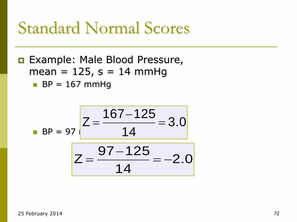
Standard Normal Scores
Example: Male Blood Pressure,mean = 125, s = 14 mmHg
BP = 167 mmHg
BP = 97 mmHg3.0
14
125167Z
2.014
12597Z
25 February 2014 73
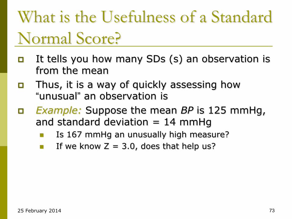
What is the Usefulness of a Standard
Normal Score? It tells you how many SDs (s) an observation is
from the mean
Thus, it is a way of quickly assessing how ―unusual‖ an observation is
Example: Suppose the mean BP is 125 mmHg, and standard deviation = 14 mmHg
Is 167 mmHg an unusually high measure?
If we know Z = 3.0, does that help us?
Descriptive Statistics II 74
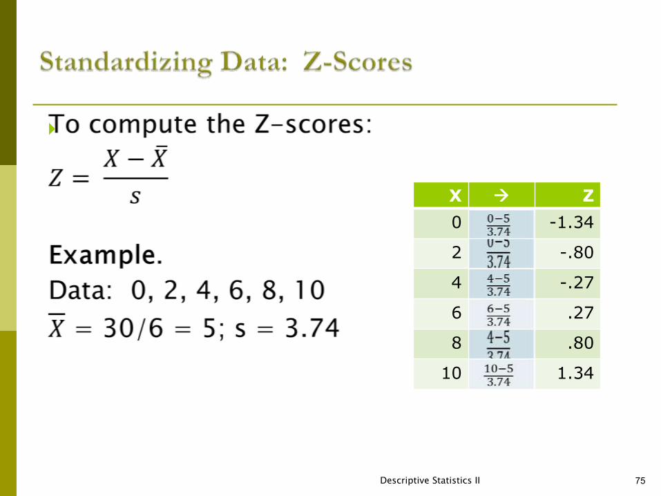
Descriptive Statistics II 75
X Z
0 -1.34
2 -.80
4 -.27
6 .27
8 .80
10 1.34

Descriptive Statistics II 76
Data: Exam Scores
Original data Change 7 to 97 Change 23 to 93
X Z X Z X Z
65 -0.45 65 -0.81 65 -1.40
73 -0.11 73 -0.38 73 -0.79
78 0.10 78 -0.10 78 -0.40
69 -0.28 69 -0.60 69 -1.09
78 0.10 78 -0.10 78 -0.40
7 -2.89 <= 97 0.94 97 1.07
23 -2.21 23 -3.12 <= 93 0.76
98 0.94 98 0.99 98 1.14
99 0.99 99 1.05 99 1.22
99 0.99 99 1.05 99 1.22
97 0.90 97 0.94 97 1.07
99 0.99 99 1.05 99 1.22
75 -0.02 75 -0.27 75 -0.63
79 0.14 79 -0.05 79 -0.32
85 0.40 85 0.28 85 0.14
63 -0.53 63 -0.92 63 -1.56
67 -0.36 67 -0.70 67 -1.25
72 -0.15 72 -0.43 72 -0.86
73 -0.11 73 -0.38 73 -0.79
93 0.73 93 0.72 93 0.76
95 0.82 95 0.83 95 0.91
Mean 75.57 Mean 79.86 Mean 83.19
s 23.75 s 18.24 s. 12.96
No matter what you are measuring, a Z-score of more than +5 or less than – 5 would indicate a very, very unusual score.
For standardized data, if it is normally distributed, 95% of the data will be between ±2 standard deviations about the mean.
If the data follows a normal distribution, 95% of the data will be between -1.96 and +1.96.
99.7% of the data will fall between -3 and +3.
99.99% of the data will fall between -4 and +4.
Worst case scenario: 75% of the data are between 2 standard deviations about the mean.
77
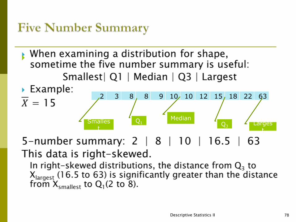
Descriptive Statistics II 78
2 3 8 8 9 10 10 12 15 18 22 63
Smallest
Largest
MedianQ1 Q3
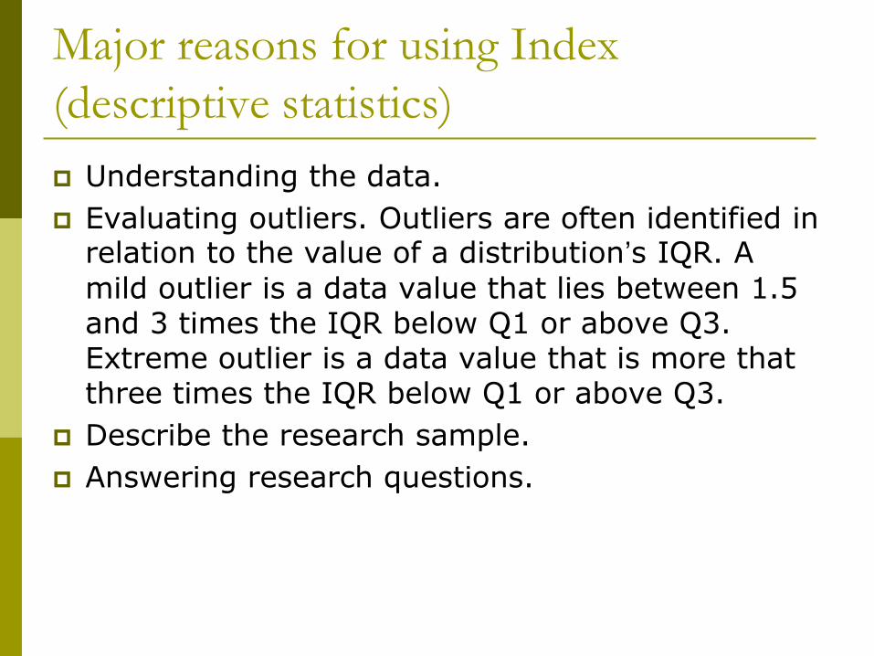
Major reasons for using Index
(descriptive statistics)
Understanding the data.
Evaluating outliers. Outliers are often identified in relation to the value of a distribution’s IQR. A
mild outlier is a data value that lies between 1.5 and 3 times the IQR below Q1 or above Q3. Extreme outlier is a data value that is more that three times the IQR below Q1 or above Q3.
Describe the research sample.
Answering research questions.