Derivatives Pricing and Stochastic Calculus

Romuald ElieLAMA, CNRS UMR 8050

Universite Paris-Est Marne-La-Vallee

elie @ ensae.fr

Idris KharroubiCEREMADE, CNRS UMR 7534,

Universite Paris Dauphine

kharroubi @ ceremade.dauphine.fr

October 11, 2013

Contents

1 Probability reminder 31.1 Generalities on probability spaces . . . . . . . . . . . . . . . . . . . . . . . . . 3

1.1.1 Measure theory and probability space . . . . . . . . . . . . . . . . . . . 31.1.2 Moments . . . . . . . . . . . . . . . . . . . . . . . . . . . . . . . . . . 5

1.2 Gaussian random variables . . . . . . . . . . . . . . . . . . . . . . . . . . . . . 61.2.1 Scalar Gaussian variables . . . . . . . . . . . . . . . . . . . . . . . . . 61.2.2 Multivariate Gaussian variables . . . . . . . . . . . . . . . . . . . . . . 6

1.3 Conditional expectation . . . . . . . . . . . . . . . . . . . . . . . . . . . . . . . 71.3.1 Sub-σ-algebra and conditioning . . . . . . . . . . . . . . . . . . . . . . 71.3.2 Computations of conditional expectations . . . . . . . . . . . . . . . . . 8

2 Arbitrage theory 92.1 Assumptions on the market . . . . . . . . . . . . . . . . . . . . . . . . . . . . . 92.2 The notion of arbitrage . . . . . . . . . . . . . . . . . . . . . . . . . . . . . . . 92.3 Portfolio comparison under (NFL) . . . . . . . . . . . . . . . . . . . . . . . . . 102.4 Call-Put parity relation . . . . . . . . . . . . . . . . . . . . . . . . . . . . . . . 112.5 Valuation of a forward contract . . . . . . . . . . . . . . . . . . . . . . . . . . 122.6 Exercises . . . . . . . . . . . . . . . . . . . . . . . . . . . . . . . . . . . . . . 13

2.6.1 Put and Call options . . . . . . . . . . . . . . . . . . . . . . . . . . . . 132.6.2 Currency forward contract . . . . . . . . . . . . . . . . . . . . . . . . . 13

3 Binomial model with a single period 153.1 Probabilistic model for the market . . . . . . . . . . . . . . . . . . . . . . . . . 153.2 Simple portfolio strategy . . . . . . . . . . . . . . . . . . . . . . . . . . . . . . 173.3 Risk neutral probability . . . . . . . . . . . . . . . . . . . . . . . . . . . . . . . 183.4 Valuation and hedging of contingent claims . . . . . . . . . . . . . . . . . . . . 203.5 Exercices . . . . . . . . . . . . . . . . . . . . . . . . . . . . . . . . . . . . . . 21

3.5.1 Pricing of a call and a put option at the money . . . . . . . . . . . . . . . 213.5.2 Binomial tree with a single period . . . . . . . . . . . . . . . . . . . . . 22

4 Binomial model with multiple periods 234.1 Some facts on discrete time processes and martingales . . . . . . . . . . . . . . 23

1

4.2 Market model . . . . . . . . . . . . . . . . . . . . . . . . . . . . . . . . . . . . 244.3 Portfolio strategy . . . . . . . . . . . . . . . . . . . . . . . . . . . . . . . . . . 264.4 Arbitrage and risk neutral probability . . . . . . . . . . . . . . . . . . . . . . . . 274.5 Duplication of contingent claims . . . . . . . . . . . . . . . . . . . . . . . . . . 304.6 Valuation et hedging of contingent claims . . . . . . . . . . . . . . . . . . . . . 324.7 Exercices . . . . . . . . . . . . . . . . . . . . . . . . . . . . . . . . . . . . . . 33

4.7.1 Martingale transforms . . . . . . . . . . . . . . . . . . . . . . . . . . . 334.7.2 Trinomial model . . . . . . . . . . . . . . . . . . . . . . . . . . . . . . 34

5 Stochastic Calculus with Brownian Motion 355.1 General facts on random processes . . . . . . . . . . . . . . . . . . . . . . . . . 35

5.1.1 Random processes . . . . . . . . . . . . . . . . . . . . . . . . . . . . . 355.1.2 Lp spaces . . . . . . . . . . . . . . . . . . . . . . . . . . . . . . . . . . 355.1.3 Filtration . . . . . . . . . . . . . . . . . . . . . . . . . . . . . . . . . . 365.1.4 Martingale . . . . . . . . . . . . . . . . . . . . . . . . . . . . . . . . . 375.1.5 Gaussian processes . . . . . . . . . . . . . . . . . . . . . . . . . . . . . 39

5.2 Brownian motion . . . . . . . . . . . . . . . . . . . . . . . . . . . . . . . . . . 395.3 Total and quadratic variation . . . . . . . . . . . . . . . . . . . . . . . . . . . . 425.4 Stochastic integration . . . . . . . . . . . . . . . . . . . . . . . . . . . . . . . . 465.5 Ito’s formula . . . . . . . . . . . . . . . . . . . . . . . . . . . . . . . . . . . . . 565.6 Ito’s processes . . . . . . . . . . . . . . . . . . . . . . . . . . . . . . . . . . . . 595.7 Stochastic differential equation . . . . . . . . . . . . . . . . . . . . . . . . . . . 635.8 Exercices . . . . . . . . . . . . . . . . . . . . . . . . . . . . . . . . . . . . . . 64

5.8.1 Brownian bridge . . . . . . . . . . . . . . . . . . . . . . . . . . . . . . 645.8.2 SDE with affine coefficients . . . . . . . . . . . . . . . . . . . . . . . . 655.8.3 Ornstein-Ulhenbeck process. . . . . . . . . . . . . . . . . . . . . . . . . 65

6 Black & Scholes Model 666.1 Assumptions on the market . . . . . . . . . . . . . . . . . . . . . . . . . . . . . 666.2 Probabilistic model for the market . . . . . . . . . . . . . . . . . . . . . . . . . 666.3 Risk neutral probability . . . . . . . . . . . . . . . . . . . . . . . . . . . . . . . 686.4 Self-financing portfolios . . . . . . . . . . . . . . . . . . . . . . . . . . . . . . 716.5 Duplication of a financial derivative . . . . . . . . . . . . . . . . . . . . . . . . 746.6 Black & Scholes formula . . . . . . . . . . . . . . . . . . . . . . . . . . . . . . 776.7 Greeks . . . . . . . . . . . . . . . . . . . . . . . . . . . . . . . . . . . . . . . . 796.8 Exercices . . . . . . . . . . . . . . . . . . . . . . . . . . . . . . . . . . . . . . 80

6.8.1 Option valuation in the Black & Scholes model . . . . . . . . . . . . . . 806.8.2 Put option with mean strike . . . . . . . . . . . . . . . . . . . . . . . . 816.8.3 Asian Option . . . . . . . . . . . . . . . . . . . . . . . . . . . . . . . . 82

2

Chapter 1

Probability reminder

1.1 Generalities on probability spaces

1.1.1 Measure theory and probability space

Definition 1.1.1 (σ-algebra). Let Ω be a set with P(Ω) the class of all subsets of Ω. A σ-algebraA on Ω is a sub-class of P(Ω) satisfying

– Ω, ∅ ∈ A,

– if A ∈ A then Ac := ω ∈ Ω : ω /∈ A ∈ A,

– if (An)n≥1 is a sequence of elements of P(A) such that

An ∈ A and An ⊂ An+1

for all n ≥ 1 then ⋃n≥1

∈ A .

The couple (Ω,A) with A such a σ-algebra on Ω is called a measurable space.

Proposition 1.1.1. Let C be a class of elements of P(Ω). Then there exists a smallest σ-algebraσ(C) containing C. It is given by

σ(C) =⋂

T σ−algebra : C⊂T

T .

σ(C) is called the σ-algebra generated by C.

Example 1.1.1. If we take Ω = R and C = [x,∞) , x ∈ R then σ(X) is called the Borelσ-algebra and is denoted by B(R). Il is also the σ-algebra generated by the open (resp. closed)subsets of R.

3

Definition 1.1.2 (Probability measure). Let (Ω,A) be a measurable space. A probability measureP on (Ω,A) is a function

P : A → [0, 1]

such that for any sequence (An)n≥1 of elements of A satisfying

Ai ∩ Aj = ∅ , for any i 6= j ,

we have

P( ⋃n≥1

An

)= lim

N→∞

N∑n=1

P(An)

The triplet (Ω,A,P) is called a probability space.

Definition 1.1.3 (independence). Let (Ω,A,P) be a probability space

(i) Let A and B two elements of A. We say that A and B are independent if

P(A,B) := P(A ∩B) = P(A)× P(B) .

(ii) Let B and C be two sub-σ-algebra of A. We say that B and C are independent if any B ∈ Band C ∈ C are independent.

Definition 1.1.4 (Measurability and random variables). Let (Ω,A,P) be a probability space. Afunction X : Ω→ R is A-measurable if for any x ∈ R we have

X−1([x,+∞)

):=

ω ∈ Ω : X(ω) ≥ x

∈ A .

A random variable X on the probability space (Ω,A,P) is an A-measurable function.

Proposition 1.1.2. Let (Ω,A,P) be a probability space andX be a random variable on (Ω,A,P).Denote by σ(X) the σ-algebra σ

(X−1([x,+∞) : x ∈ R

)(see Proposition 1.1.1) . Then σ(X)

is the smallest sub-σ-algebra of A such that X is σ(X)-measurable.

Definition 1.1.5. Let X and Y be two random variables defined on a probability space (Ω,A,P).We say that X and Y are independent if σ(X) and σ(Y ) are independent.

Proposition 1.1.3. Let X and Y be two random variables on a probability space (Ω,A,P). Yis σ(X)-measurable if and only if it can be written f(X) with f : R → R a B(R)-measurablefunction.

Proof. Suppose that Y = f(X). Then, for any borel subset B of R we have

f(X)−1(B) = X−1(f−1(B)

)∈ σ(X) .

4

Conversly, if Y is the indicator function of a σ(X)-measurable set A, A can then be writtenA = X−1(B) for B ∈ B(Rd) and, we have

Y = 1A = 1X−1(B) = 1B(X) ,

and the identification Y = f(X) holds with f = 1B . if Y is a finite sum of indicator functions1Ai with Ai = σ(X), Ai can then be written Ai = X−1(Bi) for Bi ∈ B(R) andthe equality holdswith f =

∑i 1Bi convient. If Y is positive, it can be written as an increasing limit of random

variables Yn which are finite sum of indicator functions. We then have Yn = fn(X) and we getY = f(X) with f = limfn. If Y is not positive, we apply the previous result to its positive andnegative parts.

1.1.2 Moments

Definition 1.1.6. Let X be a positive random variable on a probability space (Ω,A,P). Theexpectation E[X] of X is defined by

E[X] =

∫Ω

X(ω)dP(ω) .

LetX be a random variable such that E[|X|] < +∞ (we say thatX is integrable). The expectationE[X] of X is defined by

E[X] = E[X+]− E[X−] ,

where X+ and X− are the random variables defined by

X+ = max(X, 0) and X− = max(−X, 0)

Definition 1.1.7. For p ≥ 1, we define the space Lp(Ω,A,P) (or Lp(Ω) for short) by

Lp(Ω) =X random variable on (Ω,A,P) such that E

[|X|p

]< ∞

.

Proposition 1.1.4. For p ≥ 1, the space Lp(Ω) endowed with the norm ‖ · ‖p defined by

‖X‖p =(E[|Xp|]

)p, X ∈ Lp(Ω)

is a Banach (i.e. complete vector) space.

Proposition 1.1.5 (Jensen Inequality). Let X be a random variable and ϕ : R → R be a convexfunction. Suppose that E[|ϕ(X)|] <∞, then we have

ϕ(E[X]

)≤ E

[ϕ(X)

].

Definition 1.1.8. Let (Xn)n be a sequence of random variables and X random variable on(Ω,A,P). We say that Xn converges P-a.s. to X and we write Xn → X P-a.s. if

P(ω ∈ Ω : Xn(ω) −→ X(ω) as n→∞

)= 1

5

Theorem 1.1.1 (Dominated Convergence Theorem). Let Let (Xn)n be a sequence of randomvariables and X random variable on (Ω,A,P) such that X ∈ Lp(Ω) and Xn ∈ Lp(Ω) for all n.Suppose that there exists a random variable Y ∈ Lp(Ω) such that |X| ≤ Y and |Xn| ≤ Y . If

Xn −→ X as n→ +∞ P− a.s.

then

Xn −→ X as n→ +∞ in Lp(Ω) .

1.2 Gaussian random variables

We fix in the rest of this chapter a probability space (Ω,A,P).

1.2.1 Scalar Gaussian variables

Definition 1.2.9. A real random variable X is a standard Gaussian random variable if it admitsthe density fX given by

fX(x) =1√2π

exp(− x2

2

), x ∈ R .

We recall that a random variable X admits a density f if for any Borel bounded function ϕ wehave

E[ϕ(X)

]=

∫Rϕ(x)f(x)dx .

We also notice that for a standard Gaussian random variable X we have E[X] = 0 and E[X2] = 1.

Definition 1.2.10. Letm and σ > 0 be two constants. A random variable Y is a Gaussian randomvariable with meanm and variance σ2 if the random variable Y−m

σis a standard Gaussian random

variable. We then write Y ∼ N (m,σ2).

If Y ∼ N (m,σ2) then Y admits the density fY given by

fY (y) =1√

2πσ2exp

(− |y −m|

2

2σ2

), x ∈ R .

Definition 1.2.11.

1.2.2 Multivariate Gaussian variables

Definition 1.2.12. A random vector (X1, . . . , Xn) is a Gaussien vector if any linear combinationof the components Xi is a Gaussian random variable i.e. the random variable 〈a,X〉 defined by

〈a,X〉 :=n∑k=1

aiXi

is a Gaussian random variable for all a = (a1, . . . , an) ∈ Rn.

6

We now give two useful properties related to Gaussian vectors.

Proposition 1.2.6. Let (X1, . . . , Xn) be a Gaussian vector. The components Xi and Xj are inde-pendent if and only if cov(Xi, Xj) = 0 for any i, j ∈ 1, . . . , n.

Proposition 1.2.7. LetX = (X1, . . . , Xn) be a random vector such that the componentsX1, . . . , Xn

are independent and follows Gaussian laws. Then X is a Gaussian vector

Remark 1.2.1. One should take care about the fact that it is possible to have Gaussian randomvariables X1 and X2 which are not independent and satisfy cov(X1, X2) = 0.

1.3 Conditional expectation

1.3.1 Sub-σ-algebra and conditioning

Theorem 1.3.2. Let B be a sub-σ algebra of A. For any integrable random variable X , thereexists an integrable B-measurable random variable Y such that

E[1BX

]= E

[1BY

]for any B ∈ B. If Y is another random variable with these properties we have Y = Y , P-a.s.

The almost surely uniquely defined random variable Y given by the previous theorem is calledthe conditional expectation ofX given B and is denoted by E[X|B]. This conditional expectationsatisfies the following properties.

Proposition 1.3.8. Let B be a sub-σ algebra of A.

(i) If X is an integrable B-measurable random variable we have

E[X|B] = X .

(ii) If X is a random variable and Za bounded B-measurable random variable we have

ZE[X|B

]= E

[ZX|B

].

In particular, we have

E[ZE[X|B]

]= E

[ZX

].

(iii) Linearity: if X1 and X1 are two random variables and a1 and a2 two constants we have

E[X1a1 +X2a2|B

]= a1E

[X1|B

]+ a2E

[X2|B

].

(iv) If C is a sub-σ-algebra of B and X a random variable we have

E[E[X|B]|C

]= E

[X|C

].

7

(v) Conditional Jensen Inequality: if ϕ : R → R is a convex function X a random variablesuch that ϕ(X) is integrable we have

E[ϕ(X)|B

]≤ ϕ

(E[X|B

]).

(vi) Conditional dominated convergence theorem: Let (Xn)n be a sequence of random variablesand X and Y two random variables such that

|Xn| ≤ Y , for all n ≥ 0 ,

and

Xn −→ X as n→ +∞ P− a.s.

then if Y ∈ Lp(Ω) we have

E[Xn|B

]−→ E

[X|B

]as n→ +∞ in Lp(Ω) .

1.3.2 Computations of conditional expectations

Proposition 1.3.9. Let B be a sub-σ algebra ofA. Let X be a random variable independent of B.Then we have

E[X|B

]= E

[X].

Proposition 1.3.10. Let B be a sub-σ algebra of A. Let X and Y be two random variables suchthat X is independent of B and Y is B-measurable. Then if Φ is a measurable function such thatΦ(X, Y ) is integrable we have

E[Φ(X, Y )|B

]= ϕ(Y )

where the function ϕ : R→ R is defined by by

ϕ(y) = E[Φ(X, y)]

for all y ∈ R.

8

Chapter 2

Arbitrage theory

2.1 Assumptions on the market

In the sequel, we shall make the following assumptions.

– The assets are infinitely divisible: One can sell or buy an proportion of asset.

– Liquidity of the market: one can sell or buy any quantity of any asset at any time.

– One can short sell any asset.

– There is no transaction costs.

– One can borrow and lend money at the same interest rate r.

2.2 The notion of arbitrage

To model the uncertainty of financial market, we use the probability theory. We consider a proba-bility set Ω endowed with a probability measure P. We now give the definition of a portfolio.

Definition 2.2.13. A self-financing portfolio consists in a initial capital x and an investment strat-egy without bringing or consuming any wealth.

For a portfolio X , we denote by Xt its value at time t. We now consider the situation whereone can earn money with no risk of loss.

Definition 2.2.14. An arbitrage between times 0 and T is a self financing portfolio X with initialvalue X0 = 0 and such that

P(XT ≥ 0) = 1 and P(XT > 0) > 0 .

9

We now introduce an assumption which ensures that such an opportunity does not happened.

(NFL) (No Free Lunch) There is no arbitrage opportunity between times 0 and T : for any portfolioX , we have [

X0 = 0 and XT ≥ 0]⇒ P(XT > 0) = 0 .

This assumption simply means that there is no way to earn money without taking any risk. Thisassumption also correspond to the reality of the markets. Indeed, even if an arbitrage opportunityappears in a market, it is quickly taken by a trader.

2.3 Portfolio comparison under (NFL)

Proposition 2.3.11. Let X and Y be two self-financing portfolios. Under (NFL), we have

XT = YT P− a.s. =⇒ X0 = Y0 .

Proof. Suppose that X0 < Y0 and consider the following strategy. At time t = 0, we buy X , wesell Y and we put Y0 −X0 > 0 in the bank account at interest rate r. At the terminal time t = T

the portfolio value is always positive.

value at 0 value at TBuy X X0 XT

Sell Y −Y0 −YTPut the difference in the bank account Y0 −X0 > 0 (Y0 −X0)/B(0, T ) > 0

Portfolio value 0 > 0

Therefore, (NFL) implies X0 ≥ Y0. Replacing X by Y , we get X0 ≤ Y0 and X0 = Y0.

Remark 2.3.2. To construct an arbitrage opportunity we buy the cheapest portfolio and sell themost expensive one. Since the portfolios have the same terminal value, this strategy provides apositive gain.

Proposition 2.3.12. Let X and Y be two self-financing portfolios. Under (NFL), we have

XT = YT P− a.s. =⇒ Xt = Yt P− a.s.

for all t ≤ T .

This result is a direct consequence of the following proposition.

Proposition 2.3.13. Let X and Y be two self-financing portfolios. Under (NFL), we have

XT ≤ YT =⇒ Xt ≤ Yt

for all t ≤ T .

10

Proof. Fix t ≤ T and consider the following strategy:

• at time 0: we do nothing.

• at time t:

– on the set ω ∈ Ω, Xt(ω) > Yt(ω), we buy Y at price Yt, we sell X at price Xt and we putthe difference Xt − Yt > 0 in the bank account,

– on the set ω ∈ Ω, Xt(ω) ≤ Yt(ω), we do nothing.

Finaly, at time T ,

– on Xt > Yt, the portfolio contains YT − XT ≥ 0 and the positive amount in the bankaccount, thus it has a positive value,

– on Xt ≤ Yt, the portfolio value is equal to zero.

at time t t en TOn Xt > Yt Buy Y at time t Yt YT

Sell X at time t −Xt −XT

Put the difference in the bank account Xt − Yt > 0 (Xt − Yt)/B(t, T ) > 0

Portfolio value 0 > 0

On Xt ≤ Yt Portfolio value 0 0

Therefore (NFL) implies P(Xt > Yt) = 0.

2.4 Call-Put parity relation

A call option with strike K and maturity T on the underlying S is a contract that provides thepayoff (ST −K)+ =: maxST −K, 0 at time T . We denote by Ct the price of such a contract attime t.

A put option with strike K and maturity T on the underlying S is a contract that provides thepayoff (K − ST )+ =: maxK − ST , 0. We denote by Pt its price at time t.

A zero-coupon bond with maturity T is a financial product with value 1 at time T . We denote byB(t, T ) its price at time t.

We then have the following relation between C, P and B.

Proposition 2.4.14. Under (NFL), the call and put prices satisfy the parity relation

Ct − Pt = St −KB(t, T )

for all t ≤ T .

11

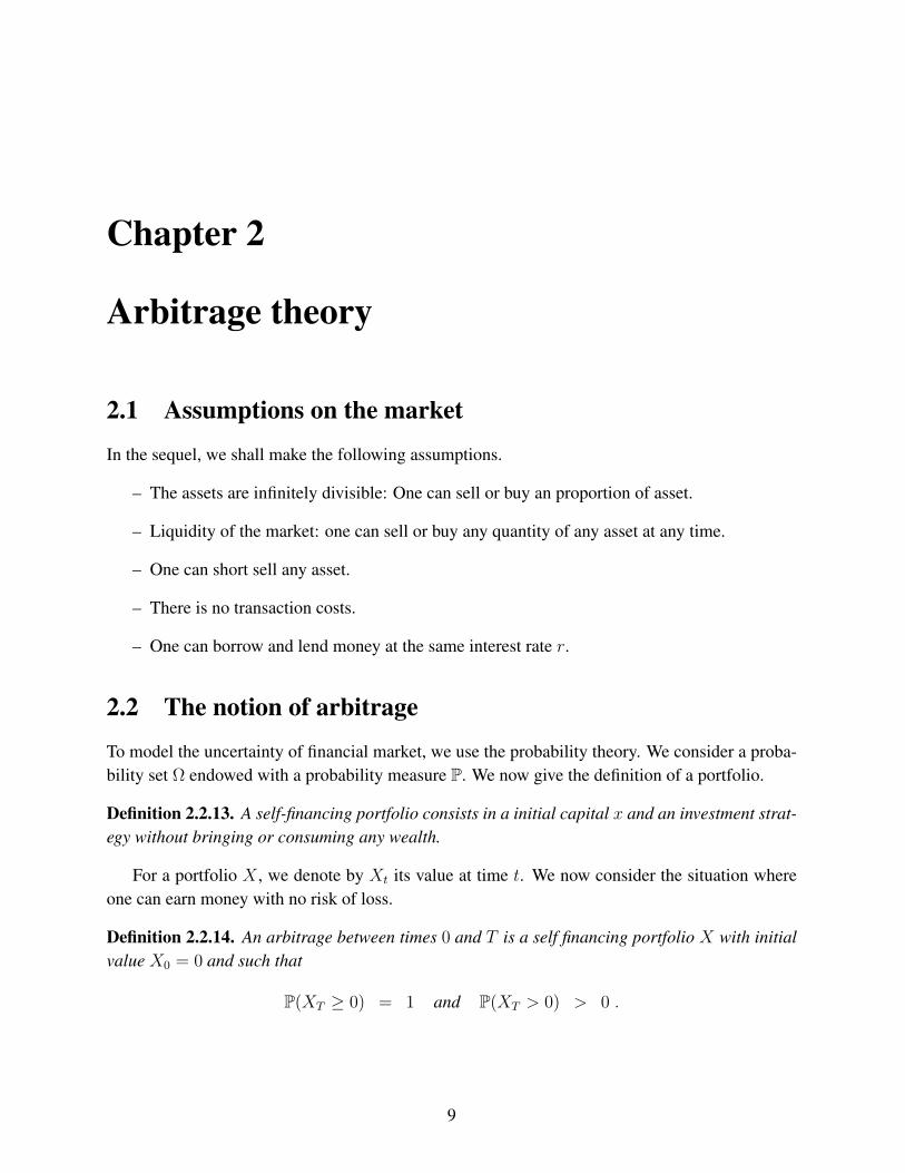
Proof. Consider the two following self-financing strategies:

at 0 at t at TPort. 1 Buy a put option at t Pt (K − ST )+

Buy the underlying asset at t St STValue Pt + St (K − ST )+ + ST

Port. 2 Buy a call option at t Ct (ST −K)+

Buy K units of zero-coupon bond at t KB(t, T ) K

Value Ct +KB(t, T ) (ST −K)+ +K

We then notice that

(K − ST )+ + ST = K 1ST≤K + ST 1K≤ST = (ST −K)+ +K .

Therefore , these two portfolios have the same terminal value. Under (NFL), we get from Propo-sition 2.3.12 that they have the same value at every time t ≤ T , which gives the call-put parityrelation.

Remark 2.4.3. This parity relation is specific to the (NFL) assumption. In particular it does notdepend no the model that we put on the market.

2.5 Valuation of a forward contract

A forward contract is a contract signed at time t = 0 between two parties to buy or sell an asset ata specified future time at a price F (0, T ) agreed upon today. There is no change of money betweenthe two parties at time t = 0.

To determine the forward price F (0, T ) we consider the two self-financing strategies:

at time 0 at time TPort. 1 Buy a unit of the underlying S at time 0 S0 ST

Sell F (0, T ) units of zero-coupons bounds at time 0 −F (0, T )B(0, T ) −F (0, T )

Value S0 − F (0, T )B(0, T ) ST − F (0, T )

Port. 2 Buy the forward contrat at time 0 0 ST − F (0, T )

Under (NFL), we get from Proposition 2.3.12

F (0, T ) =S0

B(0, T ).

Remark 2.5.4. More generally, we have

F (t, T ) =St

B(t, T )

for all t ≤ T .

12

2.6 Exercises

2.6.1 Put and Call options

We suppose that there is not any arbitratage opportunity on the market i.e. (NFL) holds. We denoteby B0 the price at time t = 0 of the riskless asset with gain 1 at maturity t = T . We also denote byC0 and P0 the respective prices at time t = 0 of a Call and a Put option on the underlying S withmaturity T and strike K.

1. Prove by an arbitrage argument that

(S0 −KB0)+ ≤ C0 ≤ S0 .

2. Deduce from the previous question that

(KB0 − S0)+ ≤ P0 ≤ KB0 .

3. Prove that the Call option price is a nonincreasing function of the strike K and a nondecreasingfunction of the maturity.

4. What can you say about the Put option price?

2.6.2 Currency forward contract

We consider on the time interval [0, T ] the market of the currency pair euro/US dollar. This marketcan be described as follows.

1. In the european economy, there is a riskless asset with continuous time interest rate rd.This european riskless asset pays 1 at maturity T , thus its price at time t is given by Bd

t =

e−rd(T−t) e for all t ∈ [0, T ].

2. In the american economy, there also exists a riskless asset with continuous time interest raterf . This american riskless asset pays 1 at maturity T, thus its price at time t is given byBft = e−rf (T−t) $ for all t ∈ [0, T ].

3. To get 1 dollar at time t ∈ [0, T ], one has to pay St.

4. Finaly, on this market there exist forward contracts for any date t ∈ [0, T ]. A forwardcontract signed at time t ∈ [0, T ] is defined by the following rules:

– no change of money at the entering date t,

– at time T , we get 1 $ and we pay Ft e, where the amount Ft is fixed at the initial timet.

1. Fix t ∈ [0, T ]. Using ST , give the pay-off a time T in euro, of the following portfoliosconstructed at time t.

13

(a) Buy Bft $ at time t. this amount is invested in the american riskless asset. Borrow FtB

dt e at

time t.

(b) Sign a forward contract at time t.

2. Give the pay-off in euro at time T of the portfolio composed by buying a forward contract withforward price F0 and the short selling at time t a forward contract with forward price Ft. By a nofree lunch argument, deduce the value f 0

t in euro at time t of the forward contract signed at time 0

as a function of Ft and F0 and then as a function of St and S0.

14

Chapter 3

Binomial model with a single period

The binomial model is very useful for the computation of prices and most of its properties can begeneralised to the continuous time case.

3.1 Probabilistic model for the market

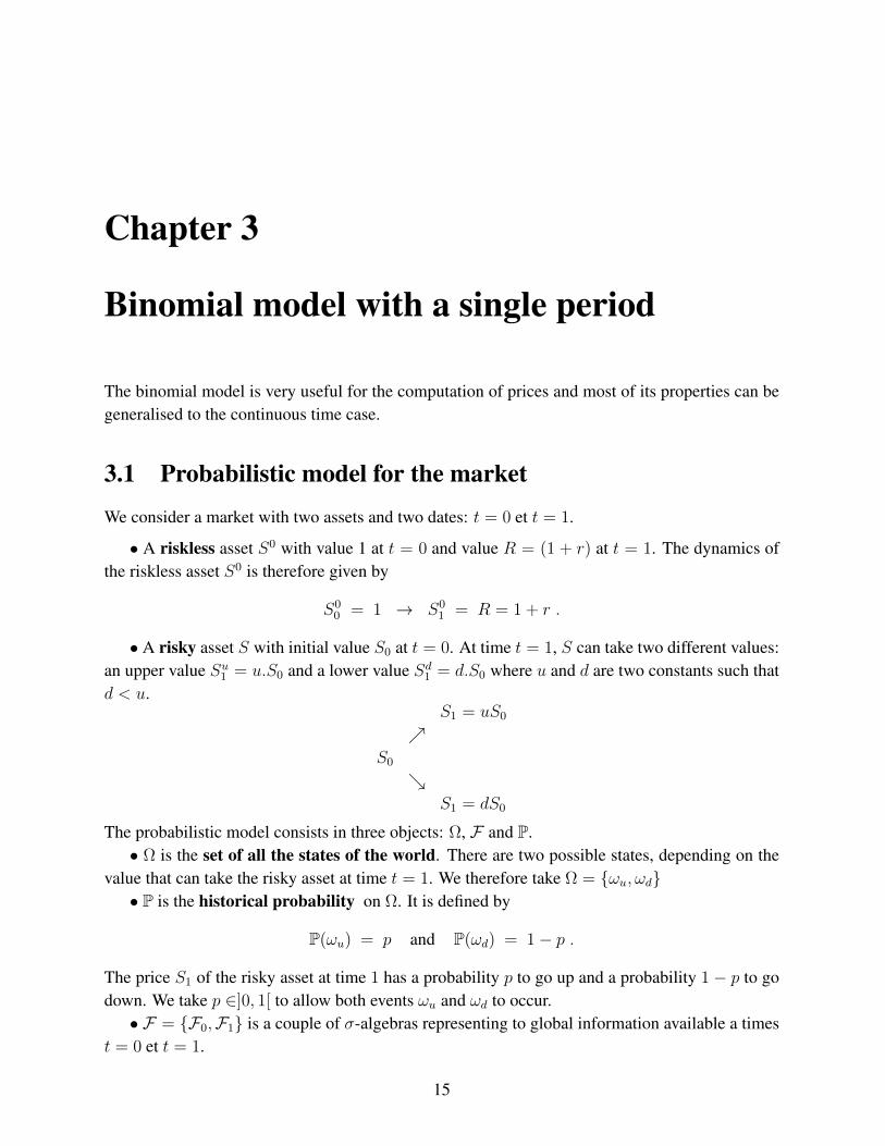
We consider a market with two assets and two dates: t = 0 et t = 1.

• A riskless asset S0 with value 1 at t = 0 and value R = (1 + r) at t = 1. The dynamics ofthe riskless asset S0 is therefore given by

S00 = 1 → S0

1 = R = 1 + r .

• A risky asset S with initial value S0 at t = 0. At time t = 1, S can take two different values:an upper value Su1 = u.S0 and a lower value Sd1 = d.S0 where u and d are two constants such thatd < u.

S1 = uS0

S0

S1 = dS0

The probabilistic model consists in three objects: Ω, F and P.• Ω is the set of all the states of the world. There are two possible states, depending on the

value that can take the risky asset at time t = 1. We therefore take Ω = ωu, ωd• P is the historical probability on Ω. It is defined by

P(ωu) = p and P(ωd) = 1− p .

The price S1 of the risky asset at time 1 has a probability p to go up and a probability 1− p to godown. We take p ∈]0, 1[ to allow both events ωu and ωd to occur.• F = F0,F1 is a couple of σ-algebras representing to global information available a times

t = 0 et t = 1.

15

– At time t = 0, there is no information, so F0 is the trivial σ-algebra:

F0 = ∅,Ω.

– At time t = 1, one knows if the the asset S went up or down:

F1 = P(Ω) = ∅,Ω, ωu, ωd.

This σ-algebra represents all the subsets of Ω that can be said to have occurred or not at timet = 1.

Remark 3.1.5. We have F0 ⊂ F1. Indeed, we get more and more information with time.

Remark 3.1.6. F1 is the σ-algebra generated by S1:

F1 = σ(S1) .

Indeed, by definition, the σ-algebra generated by S1 is the class of inverse images by S1 of Borelsubsets of R, i.e. S−1

1 (B) ,B ∈ B(R). It is also the smallest σ-algebra that makes S1 measurable.For any Borel subset B of R,

– if uS0 and dS0 belong to B, we have S−11 (B) = Ω,

– if uS0 belongs to B, we have S−11 (B) = ωu,

– if dS0 belongs to B, we have S−11 (B) = ωd,

– and if any of these two values is in B, we have S−11 (B) = ∅.

Therefore F1 is the σ-algebra generated by S1.

Definition 3.1.15. A contingent claim (or financial derivative) is an F1-measurable random vari-able.

The value of a contingent claim depends on the state of the world at time t = 1. From Propo-sition 1.1.3 and Remark 3.1.6, any contigent claim C can be written

C = φ(S1)

where φ : R→ R is a deterministic measurable function. For instance, if C is a Call option withstrike K, we have C = φ(S1) with φ : x ∈ R 7→ (x−K)+

We consider the problem of the valuation of a contingent claim at time t = 0. To this end weconstruct a hedging portfolio for our contigent claim. Under Assumption (NFL) we obtain that allthe replicating portfolios have the same initial capital which is the economic definition of the priceof the contingent claim.

16

3.2 Simple portfolio strategy

Definition 3.2.16. A simple portfolio strategy (x,∆) consists in an initial amount x and a quantity(number of units) ∆ of risky asset S. We denote by Xx,∆

t the value of the associated self-financingportfolio at time t = 0, 1.

For a simple portfolio strategy (x,∆), we have at time t = 0

Xx,∆0 = ∆S0 + (x−∆S0) 1 = x .

Since Xx,∆ is a self-financing portfolio, its value at time t = 1 is given by

Xx,∆1 = ∆S1 + (x−∆S0)R

= ∆(S1 − S0R) + xR .

Such a strategy (x,∆) is said to be simple since it consists in investing only in the assets S0 andS1.

Definition 3.2.17. A contingent claim C is said to be replicated if there exists a simple strategy(x,∆) such that Xx,∆

1 = C P-a.s.

Theorem 3.2.3. The binomial model with a single period is complete: any contingent claim C

can be replicated by a simple portfolio strategy (x,∆).

Proof. Consider a contingent claim C. We look for a couple couple (x,∆) satisfyingC(ωu) = ∆Su1 + (x−∆S0)R = xR + (u−R)∆S0 ,

C(ωd) = ∆Sd1 + (x−∆S0)R = xR + (d−R)∆S0 .

Since u > d, this system of two equations with two unknowns is invertible. It therefore admits aunique solution (x,∆) which is given by

∆ =C(ωu)− C(ωd)

(u− d)S0

and x =1

R

(R− du− d

C(ωu) +u−Ru− d

C(ωd)

).

Under (NFL) assumption, all the replication portfolios of the a contingent claim C have thesame initial value given by

C0 =1

R

(R− du− d

C1(ωu) +u−Ru− d

C1(ωd)

).

The economic definition of the price of a contingent claim at time t = 0 is therefore C0.

17

3.3 Risk neutral probability

Definition 3.3.18. A simple arbitrage opportunity is a simple portfolio strategy (x,∆) with initialamount equal to zero, x = 0, and a nonnegative terminal wealth which is positive with positiveprobability:

X0,∆1 ≥ 0 et P

[X0,∆

1 > 0]> 0

We then introduce the no free lunch assumption in this context.

(NFL’) For any simple strategy (0,∆), we have[X0,∆

1 ≥ 0 P− a.s.]

=⇒[X0,∆

1 = 0 P− a.s.]

Proposition 3.3.15. Under (NFL’) we have d < R < u.

Proof. Suppose that d ≥ R. An arbitrage strategy is then given by (0,∆) with ∆ = 1 (i.e. buyinga unit of a risky asset). Indeed, at time t = 1, we have

X0,∆1 (ωu) = S0(u−R) > 0 ,

X0,∆1 (ωd) = S0(d−R) ≥ 0 .

Suppose that u ≤ R. An arbitrage strategy is then given by (0,∆) with ∆ = −1 (i.e. selling a unitof a risky asset). Indeed, at time t = 1, we have

X0,∆1 (ωu) = S0(R− u) ≥ 0 ,

X0,∆1 (ωd) = S0(R− d) > 0 .

For a simple portfolio strategy (x,∆), let us introduce the discounted value Xx,∆ of the portfolioXx,∆ defined by

Xx,∆t :=

Xx,∆t

Rt

for t = 0, 1. We then have Xx,∆0 = x and Xx,∆

1 = ∆S1 + (x−∆S0). The self-financing conditioncan be rewritten with the discounted values under the following form:

Xx,∆1 − Xx,∆

0 = ∆(S1 − S0) .

Definition 3.3.19. A risk neutral probability is a probability measure Q defined on Ω and equiv-alent to P, under which any discounted value Xx,∆ of self-financing portfolio is a martingale,i.e.

Xx,∆0 = EQ[Xx,∆

1 ] or equivalently x =1

REQ[Xx,∆

1 ] .

18

Remark 3.3.7. Two probability measures P and Q are said to be equivalent if they have the samenegligible sets, i.e. P(A) > 0⇔ Q(A) > 0, for any event A. In the binomial , this simply meansQ(ωd) > 0 and Q(ωu) > 0.

A first result is that we cannot have multiple risk neutral probabilities.

Proposition 3.3.16. Since the market is complete, there is at most a unique risk neutral proba-bility.

Proof. Indeed, suppose that we have two risk neutral probability measures Q1 and Q2. Fix B ∈F1 = P(Ω), and consider the contingent claim C = 1B. Since the market is complete there existsa simple portfolio strategy (x,∆) that replicates C. We then get

Q1(B) = EQ1 [1B] = EQ1 [Xx∆1 ] = Rx

Q2(B) = EQ2 [1B] = EQ2 [Xx∆1 ] = Rx .

Therefore, Q1(B) = Q2(B), and since B is arbitrarily chosen in F1 we have Q1 = Q2.

Proposition 3.3.17. Suppose that d < R < u, then there exists a unique risk neutral probabilityQ.

Proof. Let us take a simple portfolio strategy (x,∆). We have the following equations:Xx,∆

1 (ωu) = ∆S1(ωu) + (x−∆S0)R = xR + (u−R)∆S0

Xx,∆1 (ωd) = ∆S1(ωd) + (x−∆S0)R = xR + (d−R)∆S0

which give

x =1

R

(u−Ru− d

Xx,∆1 (ωd) +

R− du− d

Xx,∆1 (ωu)

). (3.3.1)

Introduce the probability measure Q defined on Ω by

Q(ωu) :=R− du− d

:= q and Q(ωd) :=u−Ru− d

= 1− q .

Since d < R < u, we get q ∈]0, 1[ and Q is equivalent to P. From the definition of Q, equationrewrites

x =1

R

(Q(ωd)X

x,∆1 (ωd) + Q(ωu)X

x,∆1 (ωu)

)=

1

REQ[Xx,∆

1 ] .

The uniqueness of Q follows from Proposition 3.3.16.

Proposition 3.3.18. Suppose that there exists a (unique) risk neutral probability Q, then assump-tion (NFL’) holds true.

19

Proof. Fix ∆ ∈ R such that X0,∆1 ≥ 0. Since Q is a risk neutral probability, we have

EQ[X0,∆1 ] = R . 0 = 0 .

So, X0,∆1 is a nonnegative random variable with expectation under Q equal to zero. Therefore

Q(X0,∆1 > 0) = 0. Since P and Q are equivalent we get P(X0,∆

1 > 0) = 0.

We have finaly proved

(NFL’) =⇒ d < R < u =⇒ There exists a unique risk neutral probabilty =⇒ (NFL’) ,

therefore, all this implications become equivalences

(NFL’) ⇔ d < R < u ⇔ There exists a unique risk neutral probabilty

3.4 Valuation and hedging of contingent claims

We can now give the definition of the price of a contingent claim.

Theorem 3.4.4. LetC be a contingent claim. Under (NFL’), all the strategies (x,∆) that replicateC have the same initial capital P0(C) given by

P0(C) =1

1 + rEQ[C] ,

where Q is the unique probability measure. P0(C) is called the price of the contingent claim C.

Proof. Let (x,∆) and (x′,∆′) be two simple strategies replicating C. Then we have

Xx,∆1 = Xx′,∆′

1 = C .

Under (NFL’), there exists a unique risk neutral probability measure Q. Since Xx,∆ and Xx′,∆′

are martingales under Q we get

x =1

1 + rEQ[Xx,∆

1 ] =1

1 + rEQ[C] ,

x′ =1

1 + rEQ[Xx′,∆′

1 ] =1

1 + rEQ[C] .

Therefore, we get x = x′.

The price P0(C) can be expressed with the parameter q as follows:

P0(C) =1

R

(q C(ωu) + (1− q)C(ωd)

)=

1

1 + rEQ[C]

20

Remark 3.4.8. The risk neutral probability does not depend on the historical probability P. There-fore,

“The price of a contingent claim does not depend on the historical probability P”.

Remark 3.4.9. To compute the price of a cotigent claim C, we only need to know the parametersr, u et d. The coefficients u et d correspond to what we call the volatility of the asset in the nextchapters.

Remark 3.4.10. In the hedging portfolio of a contigent claim C, the number ∆ of shares of S heldis given by:

∆ =C(ωu)− C(ωd)

(u− d)S0

(=

φ(Su1 )− φ(Sd1)

Su1 − Sd1

),

which is the relative variation of the contingent claim w.r.t. the risky asset S.

3.5 Exercices

3.5.1 Pricing of a call and a put option at the money

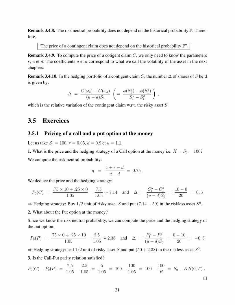
Let us take S0 = 100, r = 0.05, d = 0.9 et u = 1.1.

1. What is the price and the hedging strategy of a Call option at the money i.e. K = S0 = 100?

We compute the risk neutral probability:

q =1 + r − du− d

= 0.75 .

We deduce the price and the hedging strategy:

P0(C) =.75× 10 + .25× 0

1.05=

7.5

1.05∼ 7.14 and ∆ =

Cu1 − Cd

1

(u− d)S0

=10− 0

20= 0, 5

⇒ Hedging strategy: Buy 1/2 unit of risky asset S and put (7.14− 50) in the riskless asset S0.

2. What about the Put option at the money?

Since we know the risk neutral probability, we can compute the price and the hedging strategy ofthe put option:

P0(P ) =.75× 0 + .25× 10

1.05=

2.5

1.05∼ 2.38 and ∆ =

P u1 − P d

1

(u− d)S0

=0− 10

20= −0, 5

⇒ Hedging strategy: sell 1/2 unit of risky asset S and put (50 + 2.38) in the riskless asset S0.

3. Is the Call-Put parity relation satisfied?

P0(C)− P0(P ) =7.5

1.05− 2.5

1.05=

5

1.05= 100− 100

1.05= 100− 100

R= S0 −KB(0, T ) .

21

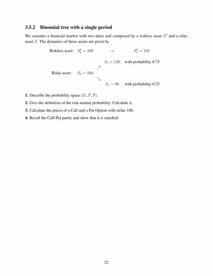
3.5.2 Binomial tree with a single period

We consider a financial market with two dates and composed by a riskless asset S0 and a riskyasset S. The dynamics of these assets are given by

Riskless asset: S00 = 100 → S0

1 = 105

S1 = 120 with probability 0.75

Risky asset: S0 = 100

S1 = 90 with probability 0.25

1. Describe the probability space (Ω,F ,P).

2. Give the definition of the risk neutral probability. Calculate it.

3. Calculate the prices of a Call and a Put Option with strike 100.

4. Recall the Call-Put parity and show that it is satisfied.

22

Chapter 4

Binomial model with multiple periods

With this model, also called Cox Ross Rubinstein model, we get similar results to those obtainedin the previous chapter for the one period binomial model.

4.1 Some facts on discrete time processes and martingales

We fix in this section a probability space (Ω,A,P).

Definition 4.1.20. A (discrete time) process is a finite sequence of random variables (Yk)0≤k≤n

defined on (Ω,A,P).

Definition 4.1.21. A (discrete time) filtration is a nondecreasing sequence (Fk)0≤k≤n of σ-algebrasincluded in A, i.e.

Fk ⊂ Fk+1 ⊂ A ,

for all k ∈ 0, . . . , n− 1.

Definition 4.1.22. A process (Yk)0≤k≤n, is adapted to the filtration F (or F-adapted) if Yk isFk-measurable for all k ≤ n.

Proposition 4.1.19. Let (Yk)0≤k≤n be an F-adapted process. Then, the random variable Yi isFk-measurable for all i ≤ k.

Proof. In terms of information, if the result of the random variable Yi is included in the informationgiven by Fi, it is included in the information given by Fk ⊃ Fi.

In the formalism of measure theory, one notice that the reciprocal image Y −1i (B) of any Borel

set B by Yi is in Fi. Since Fi ⊂ Fk for k ≥ i, we get Y −1i (B) ∈ Fk.

Definition 4.1.23. The filtration generated by a process (Yk)0≤k≤n is the smallest filtration FYsuch that (Yk)0≤k≤n is FY -adapt. It is given by

FYk := σ(Y0, . . . , Yk) ,

for all k ∈ 0, . . . , n.

23

Remark 4.1.11. A a consequence of measurability properties, a random variable isFYk -measurableif and only if it can be written as a (Borel) function of (Y0, . . . , Yk).

Definition 4.1.24. A discrete time process (Mk)0≤k≤n is an F-martingale under P if it satisfies:

(i) M is F-adapted,

(ii) E[|Mk|] <∞ for all k ∈ 0, . . . , n,

(iii) E[Mk+1|Fk] = Mk for all k ∈ 0, . . . , n− 1.

Remark 4.1.12. The process M is said to be a supermartingale (resp. submartingale) if itsatisfies conditions (i) and (ii) of the previous definition and E[Mk+1|Fi] ≤ (resp. ≥) Mk for allk ∈ 0, . . . , n− 1.

The martingale (resp. supermartingale, submartingale) property means that the best estimate(in the least-square sense) of Mk+1 given all the past is (resp. is lower than, is greater than) Mk.

Remark 4.1.13. If M is an F-martingale under P we have

E[Mk|Fi] = Mi ,

for all i ≤ k. In particular E[Mk] = M0 for all k.

4.2 Market model

We keep the same model as in the previous chapter but with n periods (n ≥ 2). We consider atime interval [0, T ] divided in n periods 0 = t0 < t1 < ... < tn = T . We suppose that the marketis composed by two assets.

– The first one is a riskless asset S0. We denote by S0tk

it value at time tk. We suppose thatthe dynamics of the process (S0

tk)0≤k≤n is given by:

S00 = 1 → S0

t1= (1 + r) → S0

t2= (1 + r)2 → . . . → S0

T = (1 + r)n .

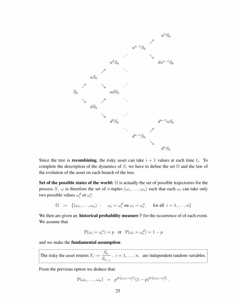
– The second one is a risky asset S. We denote by Stk it value at time tk. We fix twoconstants u > d > 0, and we suppose that the dynamics of the process (Stk)0≤k≤n is givenby the following tree:

24

unS0

un−1S0

. ..

u2S0 dun−1S0

. . .

uS0

. ..

S0 udS0

. . .

dS0

. ..

d2S0 dn−1uS0

. . . dn−1S0

dnS0

Since the tree is recombining, the risky asset can take i + 1 values at each time ti. Tocomplete the description of the dynamics of S, we have to define the set Ω and the law ofthe evolution of the asset on each branch of the tree.

Set of the possible states of the world: Ω is actually the set of possible trajectories for theprocess S. ω is therefore the set of n-tuples (ω1, . . . , ωn) such that each ωi can take onlytwo possible values ωdi or ωui .

Ω := (ω1, . . . , ωn) : ωi = ωdi ou ωi = ωui , for all i = 1, . . . , n

We then are given an historical probability measure P for the occurrence of of each event.We assume that

P(ωi = ωui ) = p et P(ωi = ωdi ) = 1− p

and we make the fundamental assumption:

The risky the asset returns Yi :=StiSti−1

, i = 1, . . . , n, are independent random variables.

From the previous option we deduce that:

P(ω1, . . . , ωn) = p#j,ωj=ωuj (1− p)#j,ωj=ωdj .

25

We can the rewrite the dynamics of the risky asset S as follow:

Sti = S0.i∏

k=1

Yk , i = 1, . . . , n ,

where Y1, . . . , Yn are independent random variable defined on Ω such that:

P(Yi = u) = P(ωi = ωui ) = p and P(Yi = d) = P(ωi = ωdi ) = 1− p .

The information available at each time ti, i = 0, . . . , n, is given by the filtration (Fti)0≤i≤n definedby

Ft0 = ∅,Ω ,

and

Fti := σ(Y1, Y2, . . . , Yi) = σ(St0 , St1 , St2 , . . . , Sti) , i = 1, . . . , n.

Thus, an Fti-measurable random variable is given by the information accumulated until time ti. Ittherefore can be written as a function of (St1 , . . . , Sti) or equivalently as a function of (Y1, . . . , Yi).

Definition 4.2.25. A contingent claim (or financial derivative) CT an FT -measurable randomvariable. Such a contigent claim can therefore be written

CT = φ(St1 , . . . , Stn) ,

with φ a Borel function.

We now look for the price of such a financial derivative. As previously, we use the (NFL)property to show that all the hedging portfolios of this contingent claim have the same initial valuewhich is the economic definition of the claim’s price.

4.3 Portfolio strategy

Definition 4.3.26. A (simple) portfolio strategy (x,∆) consists in an initial capital x and an F-adapted process (∆0, ...,∆n−1) where ∆i represents the number of shares of risky asset S held bythe investor at time ti, for i = 0, . . . , n− 1.

In the previous definition, we ask the process ∆ to be F-adapted since at each time ti, theinvestor does not have more information than Fti . Therefore, the investments done at time tishould be measurable w.r.t. the information Fti available at time ti.

Denote by Xx,∆ti the value of the portfolio with strategy (x,∆) at time ti for i = 0, . . . , n. At

time ti, the portfolio Xx,∆ contains ∆i shares of S. Therefore, it contains (Xx,∆i − ∆iSti)/S

0ti

units of the riskless asset S0. From the definition of S0, this can be written as

Xx,∆ti = ∆i Sti +

(Xx,∆ti −∆iSti)

(1 + r)i(1 + r)i .

26

We suppose that the portfolio is self-financing i.e. no bringing or consuming any wealth. Wetherefore get at time ti+1.

Xx,∆ti+1

= ∆i Sti+1+

(Xx,∆ti −∆iSti)

(1 + r)i(1 + r)i+1

Let us introduce the discounted processes:

Xx,∆ti :=

Xx,∆ti

(1 + r)iand Sti :=

Sti(1 + r)i

.

The previous equation can be rewritten as follow

Xx,∆ti = ∆i Sti + (Xx,∆

ti −∆iSti)1 , and Xx,∆ti+1

= ∆iSti+1+ (Xx,∆

ti −∆iSti) .

We then get the self-financing relation:

Xx,∆ti+1− Xx,∆

ti = ∆i(Sti+1− Sti) .

Since this equation holds for any i = 0, . . . , n− 1, we get by induction

Xx,∆ti+1

= x+i∑

k=0

∆k(Stk+1− Stk) ,

for all i = 0, . . . , n− 1.

Remark 4.3.14. From the previous equation we deduce that the portfolio value process Xx,∆ isF-adapted.

4.4 Arbitrage and risk neutral probability

Definition 4.4.27. An arbitrage opportunity is a portfolio strategy (x,∆) with initial amount equalto zero, x = 0, and a nonnegative terminal wealth which is positive with positive probability:

X0,∆tn ≥ 0 et P

[X0,∆tn > 0

]> 0 .

Recall that tn = T .

In the binomial model with multiple periods, the no arbitrage opportunity assumption takesthe following form.

(NFL’) We have the following implication

X0,∆T ≥ 0 =⇒ X0,∆

T = 0 P− a.s.

for any F-adapted process ∆ = (∆0, . . . ,∆n−1).

27

Proposition 4.4.20. Under Assumption (NFL), we have d < 1 + r < u.

Proof. Suppose for instance that 1 + r ≤ d and consider the portfolio strategy (0,∆), where∆0 = 1 and ∆i = 0 for i = 1, . . . , n (we buy the risky asset at time t0, we sell it at time t1 andwe put our gain in the riskless asset). The process ∆ is F-adapted since it is deterministic and theportfolio value at time T = tn is given by:

X0,∆T = 0 +

i∑k=0

∆k(Stk+1− Stk) = St1 − St0

From the definition of St1 , X0,∆T can take only two possible values:

(1 + r)n S0

(u

1 + r− 1

)> 0 , and (1 + r)n S0

(d

1 + r− 1

)≥ 0

with respective probabilities p > 0 and 1 − p > 0. This strategy is therefore an arbitrage oppor-tunity. In the case u ≤ 1 + r we construct an arbitrage opportunity by considering the strategy∆0 = −1 and ∆i = 0 for i = 1, . . . , n− 1.

Remark 4.4.15. As in the one period binomial model, if 1 + r ≥ u or 1 + r ≤ d one of the twoassets S0 and S always provides a better gain than the other. Therefore, this generates an arbitrageopportunity.

Remark 4.4.16. Under Assumption (NFL), there is no arbitrage opportunity on every subtree.Indeed, if there is an arbitrage opportunity on a subtree, the strategy consisting in

– doing nothing out of the subtree,

– following the arbitrage strategy on the subtree,

is a a global arbitrage opportunity, since the probability of reaching any sub tree is positive.

Following the results obtained in the previous chapter, we introduce the probability measureQ on Ω equal to the risk neutral probability for the binomial model with single period on eachone period subtree and keeping the random variables Yi independent. This probability measure istherefore given by

Q(ω1, . . . , ωn) = q#j,ωj=ωuj .(1− q)#j,ωj=ωdj with q :=(1 + r)− du− d

.

Remark 4.4.17. From the definition of the measure Q we have:

Q(Sti = uSti−1) = Q(Yi = u) = q et Q(Sti = dSti−1

) = Q(Yi = d) = 1− q

Definition 4.4.28. A risk neutral probability is a probability measure equivalent to the historicalprobability P under which any simple portfolio discounted value process is a martingale.

28

We next aim at proving that the measure Q is a risk neutral probability.

Proposition 4.4.21. S is an F-martingale under Q.

Proof. S is integrable and F-adapted. We then have

EQ[Stk+1

∣∣Ftk] =1

1 + r

(q uStk + (1− q) dStk

)=

1

1 + r

((1 + r)− du− d

u+u− (1 + r)

u− dd

)Stk

= Stk

for any k = 0, . . . , n− 1.

Proposition 4.4.22. The discounted value Xx,∆ of a portfolio with strategy (x,∆) is an F-martingale under Q.

Proof. Xx,∆ est intgrable F-adapted and

EQ[Xx,∆k+1 − X

x,∆k

∣∣Ftk] = EQ[∆k(Stk+1− Stk)

∣∣Ftk] = ∆k EQ[(Stk+1− Stk)

∣∣Ftk] = 0 .

Remark 4.4.18. The revious proposition tells us that any portfolio discounted value process isa martingale as soon as the discounted assets are martingales. This is mainly due to the factthat the number of shares of S held by the investor between tk and tk+1 is constant (from theself-financing condition) and Ftk-measurable. This property can actually be extended to sometransformation of martingales w.r.t. predictable processes called stochastic integration and whichremains a martingale as we will see in the next chapter.

Theorem 4.4.5. Suppose that d < 1 + r < u. Then there exists a risk neutral probability (Q).

Proof. We juste have seen that Xx,∆ is anF-martingale under Q for any strategy (x,∆). MoreoverQ is equivalent to P. Indeed since d < R < u, q and (1−q) are positive. Therefore Q(ω1, . . . , ωn)

is positive for any (ω1, . . . , ωn) ∈ Ω.

We now focus on the link between the existence of a risk neutral probability Q and Assumption(NFL).

Proposition 4.4.23. Suppose that there exists a risk neutral probability. Then Assumption (NFL’)is satisfiyed.

Proof. Let Q be a risk neutral probability measure and (0,∆) a strategy such that ,

X0,∆T ≥ 0

Since Q is a risk neutral probability, we have

EQ[X0,∆T

]= (1 + r)nX0,∆

0 = 0

29

Hence, we obtain

Q(X0,∆T = 0) = 1 .

Thus X0,∆T = 0 Q-a.s. and also P-a.s. since Q and P are equivalent

We therefore get the same result as in the binomial model with a single period:

(NFL’) ⇔ d < R < u ⇔ there exists a unique risk neutral probability.

At each time ti the value of a portfolio with strategy (x,∆)and with terminal value Xx,∆T is

given by

Xx,∆ti =

1

(1 + r)n−iEQ[Xx,∆

T

∣∣Fi] .Once we have a hedging portfolio for a contingent claim, we get from (NFL’) that its value

at any time ti time is given by the conditional expectation given Fti of the discounted contingentclaim under the risk neutral probability. We now concentrate on the existence of such a hedgingportfolio.

4.5 Duplication of contingent claims

Theorem 4.5.6. any contingent claim C is duplicable by a portfolio strategy (x,∆) i.e. thereexists a strategy (x,∆) such that Xx,∆

T = C. The market is said to be complete.

Analysis of the problem. We look for a portfolio strategy (x,∆) that replicates the contigentclaim C at time T . Since C is Ftn-measurable, it can be rewritten φ(St1 , ..., Stn) for some borelfuction φ. We therefore look for (x,∆) such that

Xx,∆tn = φ(St1 , ..., Stn) .

Since any discounted portfolio value process is a martingale under the risk neutral probability Qthe hedging portfolio process Xx,∆ satisfies

Xx,∆tk

=1

(1 + r)n−kEQ[φ(St1 , ..., Stn)

∣∣Ftk] , k = 0, . . . , n .

In particular, its initial value x is necessarily given by

x :=1

(1 + r)nEQ[φ(St1 , . . . , Stn)

].

30

We then notice that 1(1+r)n−k

EQ[φ(St1 , ..., Stn)|Ftk ], as an Ftk-measurable random variable, can berewritten as Vk(St1 , . . . , Stk) with Vk a deterministic (i.e. nonrandom) function. We then have

Vk(St1 , . . . , Stk) :=1

(1 + r)n−kEQ[φ(St1 , . . . , Stn)

∣∣Ftk] , k = 0, . . . , n .

In the previous chapter, we have seen that in the hedging portfolio, the number of shares of therisky asset held by the investor is equal to the relative variation of the contingent claim value w.r.t.the risky asset. We then propose the hedging process ∆ defined by

∆k :=Vk+1(St1 , . . . , Stk , u.Stk) − Vk+1(St1 , . . . , Stk , d.Stk)

u.Stk − d.Stk,

for all k ∈ 1, . . . , n − 1. We notice that this process ∆ is F-adapted. Therefore (x,∆) definesune a simple portfolio strategy.

Solution of the problem. We now prove that the strategy (x,∆) defined previously is a hedgingstrategy for the contingent claim C. To this end, we prove by induction that

Xx,∆tk

= Vk(St1 , . . . , Stk)

for all k ∈ 0, . . . , n.

• By construction of the strategy (x,∆), we have

x :=1

(1 + r)nEQ[φ(St1 , . . . , Stn)

]= V0 .

Thus the result holds true for k = 0.

• Suppose that the result holds true for k and let us prove it for k + 1. We first notice that

Xx,∆tk

= Vk(St1 , . . . , Stk)

=1

(1 + r)n−kEQ [φ(St1 , . . . , Stn)

∣∣Ftk]=

1

(1 + r)EQ[EQ[

1

(1 + r)n−(k+1)φ(St1 , . . . , Stn)

∣∣Ftk+1

]|Ftk

]=

1

(1 + r)EQ[Vk+1(St1 , . . . , Stk+1

)∣∣Ftk]

=1

(1 + r)EQ[Vk+1(St1 , . . . , Stk , u Stk)1Xk+1=u

+Vk+1(St1 , . . . , Stk , d Stk)1Xk+1=d∣∣Ftk]

=1

(1 + r)

Q(Xk+1 = u).Vk+1(St1 , . . . , Stk , u Stk)

+Q(Xk+1 = d).Vk+1(St1 , . . . , Stk , d Stk)

=1

(1 + r)

q.Vk+1(St1 , . . . , Stk , u Stk) + (1− q).Vk+1(St1 , . . . , Stk , d Stk)

.

31

The self-financing condition writes

Xx,∆tk+1

= Xx,∆tk

+ ∆k(Stk+1− Stk) .

Writing the undiscounted value we get

Xx,∆tk+1

= q.Vk+1(St1 , . . . , Stk , u Stk) + (1− q).Vk+1(St1 , . . . , Stk , d Stk) +

Vk+1(St1 , . . . , Stk , u Stk) − Vk+1(St1 , . . . , Stk , d Stk)

uStk − d Stk

(Stk+1

− (1 + r)Stk).

Replacing Stk+1by Yk+1 Stk and q by 1+r−d

u−d , we deduce

Xx,∆tk+1

= Vk+1(St1 , . . . , Stk , u Stk)Yk+1 − du− d

+ Vk+1(St1 , . . . , Stk , d Stk)u− Yk+1

u− d.

Since Yk+1 takes only the values d and u, we get alors

Xx,∆tk+1

= Vk+1(St1 , . . . , Stk , Yk+1 Stk) = Vk+1(St1 , . . . , Stk , Stk+1) ,

which concludes the induction.

A consequence of the completeness of the market is the unicity of the risk neutral probabilitymeasure.

Proposition 4.5.24. Since the market is complete there is at most one risk neutral probabilitymeasure.

Proof. Let Q1 and Q2 be two risk neutral probability measures. For any B ∈ FT = P(Ω), 1B isa contingent claim since it is FT -measurable. It can therefore be duplicated by a simple strategy(x,∆) and we have

Q1(B) = EQ1 [1B] = (1 + r)nx = EQ2 [1B] = Q2(B) .

Therefore Q1 = Q2.

4.6 Valuation et hedging of contingent claims

Theorem 4.6.7. LetC be a contingent claim. Under (NFL’), all the strategies (x,∆) that replicateC have the same initial capital P0(C) given by

P0(C) =1

(1 + r)nEQ[C] ,

where Q is the unique probability measure. P0(C) is called the price of the contingent claim C.

32

Proof. Let (x,∆) and (x′,∆′) be two simple strategies replicating C. Then we have

Xx,∆tn = Xx′,∆′

tn = C .

Under (NFL’), there exists a unique risk neutral probability measure Q. Since Xx,∆ and Xx′,∆′

are martingales under Q we get

x =1

(1 + r)nEQ[Xx,∆

tn ] =1

(1 + r)nEQ[C] ,

x′ =1

(1 + r)nEQ[Xx′,∆′

tn ] =1

(1 + r)nEQ[C] .

Therefore, we get x = x′. Finally, since the market is complete such a replicating strategy exists.

Remark 4.6.19. As in the binomial model with a single period the price of the contingent claimdepends only on its payoff,u, r et d. In particular the price does not depend on the historicalprobability P !!!

To remember:- Le price of a contingent claim can be written as the expectation of the discounted gain un-der the risk neutral probability Q.- Under the risk neutral probability, the discounted values of simple self-financing portfoliosare martingales.

In the case where n goes to infinity, and for a good choice of the parameters u d and r, we canprove that this model converges to a continuous time model called the Black & Scholes model. Tostudy such a model, we need to define similar objects in continuous time. This will be done in thenext chapter through the stochastic calculus theory.

4.7 Exercices

4.7.1 Martingale transforms

Let (Xk)0≤k≤n be an F-martingale and (Hk)0≤k≤n−1 be a bounded F-adapted process. We definethe process (Mk)0≤k≤n by M0 = x and

Mk := x+k∑i=1

Hi−1(Xi −Xi−1) , 1 ≤ k ≤ n .

1. Prove that the process M is an F-martingale.

2. In the binomial model with n periods if the discounted risky asset is a martingale under the riskneutral probability, what can you say about the self financing strategies?

33

4.7.2 Trinomial model

We consider an extended version of the Cox Ross Rubinstein model allowing the asset price totake three different values at each time step.We suppose that there are n periods and that the market is composed by two assets.

– The first one is a riskless asset S0. We denote by S0tk

it value at time tk. We suppose thatthe dynamics of the process (S0

tk)0≤k≤n is given by:

S00 = 1 → S0

t1= (1 + r) → S0

t2= (1 + r)2 → . . . → S0

T = (1 + r)n .

– The second one is a risky asset S. We denote by Stk it value at time tk. We fix threeconstants u > m > d > −1, and we suppose that the dynamics of the process (Stk)0≤k≤n isgiven by

Stk = YkStk−1, 1 ≤ k ≤ n ,

where (Yk)1≤k≤n is an IID sequence of random variable with law

P(Y1 = u) = pu, P(Y1 = d) = pd and P(Y1 = m) = pm := 1− pu − pd ,

with pu, pm, pd ∈ (0, 1).

1. (a) Suppose that 1 + r ≤ d. Construct an arbitrage opportunity.

(b) Suppose that 1 + r ≥ u. Construct an arbitrage opportunity.

(c) Give a necessary condition to ensure the viability of the market.

2. We look for a risk neutral probability measure. We firstly suppose that n = 1.

(a) Denote by Q such a probability measure with

Q(Y1 = u) = qu, Q(Y1 = d) = qd and Q(Y1 = m) = qm := 1− qu − qd ,

Use the martingale relation

EQ[S1

]= S0

to get an equation satisfied by (qu, qm, qd).

(b) Give the expressions of qm and qd as functions of qu, r, u, d and m.

(c) By distinguishing the cases m ≥ 1 + r and m < 1 + r prove that there exists an infinity ofrisk neutral probability under the condition u > 1 + r > d. Extend this result to a multiple periodmodel.

3. (a) Prove that the existence of a risk neutral probability measure ensures the viability of themarket.

(b) Deduce a necessary and sufficient condition for the viability of the market.

34

Chapter 5

Stochastic Calculus with Brownian Motion

We fix a complete probability space (Ω,A,P).

5.1 General facts on random processes

5.1.1 Random processes

Definition 5.1.29. A (random) processX on the probability space (Ω,A,P) is a family of randomvariables. (Xt)t∈[0,T ]. Such a process X can also be seen as a function of two variables

X :

[0, T ]× Ω → R

(t, ω) 7→ Xt(ω).

The functions t 7→ Xt(ω), for ω varying in Ω, are called the trajectories of the process X

Remark 5.1.20. Since we aim at representing the dynamic evolution of a sysem by a randomprocess X , the variable t ∈ [0, T ] correspond to the time. However, if one want to represent moregeneral systems, t can be chosen as an element of R, R2 . . . The space where X is valued can alsobe more complex than R.

Definition 5.1.30. A random process X is a continuous process its trajectories t 7→ Xt(ω) arecontinuous for almost every ω ∈ Ω, i.e.

P(ω ∈ Ω : t 7→ Xt(ω) is a continuous function

)= 1 .

5.1.2 Lp spaces

Notation: For p ∈ R+, we denote by:

Lp(Ω) :=X random variable on (Ω,A,P) such that ‖X‖p := E[|X|p]

1p <∞

35

and

Lp(Ω, [0, T ]) :=

(θs)0≤s≤T B([0, T ])⊗A-measurable process such that

‖θ‖′p := E[∫ T

0

|θs|pds]1/p

<∞

Proposition 5.1.25. The vector spaces Lp(Ω) endowed with the norm ‖ · ‖p and Lp(Ω, [0, T ])

endowed with the norm ‖ · ‖′p are Banach (i.e. complete) spaces, for all p ≥ 1. .

5.1.3 Filtration

Definition 5.1.31. A Filtration F = (Ft)t∈[0,T ] is a nondecreasing family of σ-algebras includedin A, i.e.

Fs ⊂ Ft ⊂ A

for all s, t ∈ [0, T ] such that s ≤ t.

Definition 5.1.32. A process (Xt)t∈[0,T ] is F-adapted if the random variable Xt Ft-measurablefor all t ∈ [0, T ].

Proposition 5.1.26. letX be anF-adapted process. Then the random variableXs isFt-measurablefor all s, t ∈ [0, t] such that s ≤ t.

Definition 5.1.33. The filtration generated by a process X , is the smallest filtration FX for whichX is adapted. It is given by

FXt = σ(Xs, s ≤ t)

for all t ∈ [0, T ].

We recall that a σ-algebra is complete if it contains the classN of negligible sets of (Ω,A,P)whichis defined by

N = N ⊂ Ω : ∃A ∈ A , N ⊂ A and P(A) = 0 .

Definition 5.1.34. A filtration F = (Ft)t∈[0,T ] is complete if Ft is a complete σ-algebra for allt ∈ [0, T ] (which is equivalent to say that F0 is complete).

Remark 5.1.21. To make a filtration F complete, it is sufficient to add the class of negligible setN . The result of this addition is the filtration (Ft∨N )t∈[0,T ] where the σ-algebraFt∨N is definedby

Ft ∨N = σ(A ∪N , (A,N) ∈ Ft ×N )

for all t ∈ [0, T ].The complete filtration generated by a processX is called the natural filtration of the process

X .

36

If F is complete and X and Y are two processes, we have

Xt = Yt a.s. =⇒[Xt is Ft-measurable ⇔ Yt is Ft-measurable

]for all t ∈ [0, T ].

We can then prove that, if F is complete, (Xn)n≥0 is a sequence of processes and X a process,we have[

Xnt

a.s.−→ Xt and Xnt is Ft-measurable for all n ≥ 0

]=⇒

[Xt is Ft-measurable

]for all t ∈ [0, T ].

The result holds also true for a convergence in Lp(Ω) with p ≥ 1, since we have, up to asubsequence, an a.s. convergence to the same limit, and this limit remains measurable:[

Xnt

Lp−→ Xt and Xnt is Ft-measurable for all n ≥ 0

]=⇒

[Xt is Ft-measurable

].

In the sequel, we shall only consider complete filtrationsand deal with natural filtration of processes.

5.1.4 Martingale

Definition 5.1.35. A random process M = (Mt)t∈[0,T ] is an F-martingale if

(i) M is F-adapted,

(ii) Mt ∈ L1(Ω), i.e. E[|Mt|] <∞, for all t ∈ [0, T ],

(iii) E[Mt|Fs] = Ms for all s, t ∈ [0, T ] such that s ≤ t.

A random process M is an F-supermartingale (resp. an F-submartingale) if it satisfies (i), (ii)and E[Mt|Fs] ≤Ms (resp. E[Mt|Fs] ≥Ms) for all s, t ∈ [0, T ] such that s ≤ t.

Proposition 5.1.27. Any martingale M satisfies

E[Mt] = E[M0] ,

for all t ∈ [0, T ].

Proof. Indeed, we have E[Mt] = E[E[Mt|F0]] = E[M0], for all t ∈ [0, T ].

Proposition 5.1.28. Let M be a F-martingale and φ : R → R a convexe and measurable func-tion. Suppose that φ(Mt) ∈ L1(Ω) for all t ∈ [0, T ], then Φ(M) = (φ(Mt))t∈[0,T ] is a submartin-gale.

37

Proof. Since φ is measurable, φ(M) is adapted and integrable. From conditional Jensen inequalitywe have

E[φ(Mt)|Fs] ≥ φ(E[Mt|Fs]) = φ(Ms) ,

for all s, t ∈ [0, T ] such that s ≤ t.

Proposition 5.1.29. Let M be a square integrable F-martingale (i.e. E[|Mt|2] < ∞ for allt ∈ [0, T ]). Then we have

E[|Mt −Ms|2|Fs] = E[M2t −M2

s |Fs] ,

for all s, t ∈ [0, T ] such that s ≤ t.

Proof. Using the second remarkable identity we have

E[|Mt −Ms|2|Fs] = E[|Mt|2|Fs]− 2E[MtMs|Fs] + E[|Ms|2|Fs]= E[|Mt|2|Fs]− 2MsE[Mt|Fs] + |Ms|2

= E[|Mt|2 − |Ms|2|Fs] .

We obtain that |M |2 is an F-sub-martingale.

Proposition 5.1.30 (Lp stability for martingales). Let p ≥ 1 and (Mn)n≥0 a sequence of F-martingales, such that Mn

t ∈ Lp(Ω) for any n ≥ 0 and any t ∈ [0, T ]. Suppose that the randomvariable Mn

t converges to Mt in Lp(Ω) for all t in [0, T ]. Then the process M is an F-martingaleand Mt ∈ Lp(Ω) for all t ∈ [0, T ].

Proof. We have to prove the following three assertions.

•M is F-adapted.Indeed, since Mn

t is Ft-measurable for all n ≥ 1 and the filtration F is complete, we obtain thatMt is Ft-measurable.

•Mt ∈ Lp(Ω) (hence Mt ∈ L1(Ω) ⊂ Lp(Ω)) for all t ∈ [0, T ].Fix t ∈ [0, T ]. Since Mn

t converges to Mt in Lp(Ω) we have Mt ∈ Lp(Ω).

• E[Mt|Fs] = Ms for all 0 ≤ s ≤ t ≤ T .For 0 ≤ s ≤ t ≤ T , we have

‖Mns − E[Mt|Fs]‖p = ‖E[Mn

t −Mt|Fs]‖p≤ ‖Mn

t −Mt‖p −→n→∞

0 .

Since Mns − E[Mt|Fs] converges to Ms − E[Mt|Fs] in Lp(Ω) we get E[Mt|Fs] = Ms.

38

5.1.5 Gaussian processes

We first recall the definition of Gaussian vectors presented in Section 1.2 of Chapter 1.

Definition 5.1.36. A random vector (X1, . . . , Xn) is a Gaussian vector if any linear combinationof the components Xi is a Gaussian random variable i.e. the random variable 〈a,X〉 defined by

〈a,X〉 :=n∑k=1

aiXi

is a Gaussian random variable for all a = (a1, . . . , an) ∈ Rn.

The extension of Gaussian vectors to continuous time processes leads to the following definition.

Definition 5.1.37. A random process (Xt)t∈[0,T ] is a Gaussian process of for any n ≥ 1 and anyt1, . . . , tn ∈ [0, T ], such that t1 ≤ . . . ≤ tn, the random vector (Xt1 , . . . , Xtn) is Gaussian.

5.2 Brownian motion

Some historical dates and facts.

– 1828: Robert Brown, a botanist, observed the motion of pollen particles in the water.

– 1877: Delsaux explains that this irregular motion comes from shocks of pollen particles withwater molecules.

– 1900: In his Ph.D. thesis “Theorie de la speculation”, Louis Bachelier proposed a Gaussianmodel to represent the prices of financial assets.

– 1905: Albert Einstein obtained the density of the Brownian motion and linked it with thetheory of partial differential equations. Marian Smolushowski described the Brownian mo-tion as the limit of random walks.

– 1923: Mathematical study of the Brownian motion by Norbert Wiener (proof of the exis-tence).

A Brownian motion is generally denoted by B (for Brown) or W (for Wiener).

Definition 5.2.38. let F be a complete filtration. A process B is an F-(standard) Brownianmotion if it satisfies

(i) B is F-adapted,

(ii) B0 = 0 P-a.s.,

(iii) B is continuous, i.e. t 7→ Bt(ω) is continuous for P-almost all ω ∈ Ω,

39

(iv) B has independent increments: Bt − Bs is independent of Fs for all t, s ∈ [0, T ] such thats ≤ t,

(v) B has Gaussian stationary increments: Bt −Bs ∼ N (0, t− s) for all t, s ∈ [0, T ] such thats ≤ t.

If there is no ambiguity on the filtration F that we consider, or when F is the natural filtrationof the process B, we say that B is a Brownian motion without specifying the filtration.

Theorem 5.2.8. The Brownian motion exists i.e. there exist a probability space (Ω,A,P) and aprocess B defined on (Ω,A,P) such that B is a Brownian motion.

This nontrivial result is admitted. The main difficulty is to prove the continuity. The Brownianmotion can also be constructed as a limit of discrete random walks as the time mesh goes to zero.

Proposition 5.2.31. let B be a F-Brownian motion where F is the natural filtration of B. Thenthe processes (Bt), (B2

t − t) and (eσBt−σ2t2 ) (geometric Brownian motion) are F-martingales.

Proof. This three processes are F-adapted. They also are integrable since Bt ∼ N (0, t), donc sonesprance, sa variance et sa transforme de Laplace sont finies. We finaly check the last condition.Fix s, t ∈ [0, T ] such that s ≤ t.• For the first process, we have:

E[Bt|Fs] = E[Bs|Fs] + E[Bt −Bs|Fs] = Bs + E[Bt −Bs] = Bs + 0 = Bs .

• For the second one, since B is a martingale, we get:

E[B2t −B2

s |Fs] = E[(Bt −Bs)2|Fs] = E[(Bt −Bs)

2] = V ar[Bt −Bs] = t− s .

• For the last process we get from the indenpendence of the increments of B and Proposition1.3.10

E[eλBt−

λ2t2 |Fs

]= e−

λ2t2 E

[eλ(Bt−Bs)eλBs|Fs

]= e−

λ2t2 eλBsE

[eλ(Bt−Bs)

].

Using Bt −Bs ∼ N (0, t− s), we obtain

E[eλBt−

λ2t2 |Fs

]= eλBs−

λ2s2

In order to prove that a given process is a Brownian motion we can use the following result.

Theorem 5.2.9. [Characterisation of the Brownian motion] A random process X is a Brownianmotion if and only if

(i) X is a Gaussian continuous process,

(ii) X is a centred process: E[Xt] = 0 for all t ∈ [0, T ],

40

(iii) Its covariance function is given by cov(Xs, Xt) = s ∧ t , for all s, t ∈ [0, T ].

Proof. • Suppose that X is a Brownian motion. For t1 ≤ t2 ≤ . . . ≤ tn, the vector Y =

(Bt1 , Bt2−Bt1 , . . . , Btn−Btn−1) has independent Gaussian components. From Proposition 1.2.7,it is a Gaussian vector. Since any linear combination of the Bti can be written as a linear combi-nation of the compoenents of Y , we get that ((Bt1 , Bt2 , . . . , Btn) is a Gaussian vector and that Bis a Gaussian process.

The processes B is also continuous and centered E[Bt] = E[Bt − B0] = 0, t ∈ [0, T ]. Itscovariance function is given by

Cov(Bs, Bt) = E[BsBt] = E[Bs(Bt −Bs)] + E[B2s ]

= BsE[Bt −Bs] + V ar[Bs −B0] = 0 + s = s

for all s, t ∈ [0, T ] such that s ≤ t.• Suppose now that X is a process satisfying the three conditions (i), (ii) and (iii).

We prove each property of the Brownian motion

– From (iii) we have E[X20 ] = V ar[X0] = 0, thus X0 = 0 a.s.

– X is continuous from (i),

– Fix r1 ≤ . . . ≤ rn ≤ s ≤ t. The vector (Xr1 , . . . , Xrn , Xt − Xs) is Gaussian. SinceCov(Bt −Bs, Bri) = ri ∧ s− ri ∧ t = 0, we deduce from Proposition 1.2.6 that Bt −Bs isindependent of (Br1 , . . . , Brn). Since r1, . . . , rn are arbitrarily chosen in [0, s], we get thatBt −Bs is independent of FBs = σ(Br, r ≤ s).

– For s ≤ t, Bt − Bs is a Gaussian random variable with expectation E[Bt − Bs] = 0 from(ii) and with variance:

V ar[Bt −Bs] = V ar(Bt) + V ar(Bs)− 2 cov(Bt, Bs)

= t+ s− 2 s ∧ t = t− s.

thus Bt −Bs ∼ N (0, t− s) and B has stationary increments.

Remark 5.2.22. The equivalence between the independence of Bt − Bs and σ(Bs, s ≤ t) inone hand and Bt − Bs and (Br1 , . . . , Brn) for all n and r1, . . . , rn ≤ s in the other hand is aconsequence of the monotone class theorem.

Proposition 5.2.32. Let B be a Brownian motin. Then the processes 1aBa2t and Bt+t0 − Bt are

Brownian motions.

Proof. This is a consequence of the caracterisation of the Brownian motion given by Theorem5.2.9.

41

To better understand the behaviour of the brownian motion we now give some properties of itstrajectories.(1) If B is a Brownian motion, we have

Bt

t−→t→∞

0 P− a.s.

(2) The trajectories of the Borwnian motion are continuous but anywhere differentiable.(3) If B is a Brownian motion, we have

limt→∞

Bt = limt→∞

sups∈[0,t]

Bs = +∞ and limt→∞

Bt = limt→∞

infs∈[0,t]

Bs = −∞ .

Thus the Brownian motion reach all the points almost surely.(4) The Brownian motion passes through any point an infinite number of times with full probabil-ity.(5) The Brownian motion is a Markov process:

∀s ≤ t Bt|Fslaw∼ Bt|Bs

for all s, t ∈ [0, T ] such that s ≤ t.

5.3 Total and quadratic variation

Definition 5.3.39. For t ∈ [0, T ], The infinitesimal variation of order p on [0, t] of a process Xassociated to a subdivision Πn = (tn1 , . . . , t

nn) of [0, t] is defined by

V pt (Πn) :=

n∑i=1

|Xtni−Xtni−1

|p

If V pt (Πn) has a limit in some sense (convergence Lp, a.s. convergence) as πn := ‖Πn‖∞ :=

maxi≤n |tni+1 − tni | → 0, this limit does not depend on the chosen subdivisions and is called thevariation of order p of X on [0, t] . In particular

– if p = 1, the limit is called total variation of X on [0, t],

– if p = 2, the limit is called quadratic variation of X on [0, t] and is denoted by 〈X〉t.

Remark 5.3.23. The total variation of a process X is also given by

V 1t := sup

Π subdivision of [0,T ]

n∑i=1

|Xti −Xti−1| a.s.

The total variation of X can therefore be interpreted as the length of its trajectory.

42

Proposition 5.3.33. The quadratic variation of the Brownian motion on [0, T ] is well defined inL2(Ω) i.e. the infinitesimal variation converges for the norm ‖.‖2. Its value is given by

〈B〉t = t

for all t ∈ [0, T ].Moreover, if the chosen sequence of subdivision (Πn)n are such that

∑∞n=1 πn < ∞, the

convergence holds almost surely.

Proof. The infinitesimal variation of order 2 of the Brownian motion associated to a subdivisionΠn is given by

V 2T (Πn) :=

n∑i=1

|Btni−Btni−1

|2 .

We recall that for a random variable X ∼ N (0, σ2) we have E[X2] = σ2 and V ar[X2] = 2 σ4.We then get

E[V 2T (Πn)] =

n∑i=1

E[(Btni−Btni−1

)2] =n∑i=1

(tni − tni−1) = T

and

V ar[V 2T (Πn)] =

n∑i=1

V ar[(Btni−Btni−1

)2] = 2n∑i=1

(tni − tni−1)2 ≤ 2T πn −→πn→0

0 ,

where we recall that πn := max |tni−1−tni |. Therefore we get ‖V 2T (Πn)−T‖2 = V ar[V 2

T (Πn)] −→0 as πn → 0.

Suppose now that the sequence (Πn)n is such that∑∞

n=1 πn < ∞. From Markov inequalitywe have

P(|V 2T (Πn)− T | > ε

)≤ V ar[V 2

T (Πn)]

ε≤ 2T πn

ε.

for all ε > 0. Using∑∞

n=1 πn <∞, we get∑∞

i=1 P(|V 2T (Πn)−T | > ε) <∞ for any ε > 0. From

Borel-Cantelli Lemma, we get the a.s. convergence of V 2T (Πn) to T .

Proposition 5.3.34. For any sequence of subdivisions (Πn)n satisfying∑∞

n=1 πn <∞, we have

limn→∞

V 1T (Πn) = ∞ a.s.

Thus, the total variation of the Brownian motion is given by

V 1T = sup

Πn

V 1T (Πn) = ∞ a.s.

43

Proof. let Πn be a sequence of subdivisions of [0, T ] satisfying∑∞

n=1 πn < ∞. We then have foralmost all ω ∈ Ω

V 2T (Πn)(ω) ≤ sup

|u−v|≤πn|Bu(ω)−Bv(ω)| V 1

T (Πn)(ω) (5.3.1)

Form Proposition 5.3.33 the right hand side goes to T a.s. as n goes to infinity. Since B is acontinuous process, its trajectories are uniformly continuous on the compact set [0, T ]. Therefore,the term sup|u−v|≤πn |Bu(ω) − Bv(ω)| goes to zero as n goes to infinity . From (5.3.1), we thenobtain that V 1

T (Πn)(ω) goes to∞ as n goes to zero.

We now focuss on bounded variation processes.

Definition 5.3.40. A process X is a bounded variation process on [0, T ] if V 1T (X) is bounded

P-a.s.

Proposition 5.3.35. A process is a bounded variation process if and only if it is the difference oftwo nondecreasing processes.

Proof. • Let X be a bounded variation process. Define the process X∗ by

X∗t := supΠ subdivision of [0,t]

V 1t (Π) < ∞

Then, Xt can be written

Xt =Xt +X∗t

2− X∗t −Xt

2:= X+

t − X−t

for all t ∈ [0, T ]. The processes X+t et X−t are nondecreasing since |Xt−Xs| ≥ X∗t −X∗s for all

s ≤ t.• Suppose that X = X+ −X− with X+ and X− nondecreasing. We have

n∑i=1

|Xti −Xti−1| ≤

n∑i=1

(X+ti−X+

ti−1) +

n∑i=1

(X−ti−1−X−ti )

= X+t − X+

0 + X−0 − X−t = Xt − X0

for any subdivision of [0, T ]. Therefore X is a bounded variation process.

Proposition 5.3.36. Let X be a continuous bounded variation process. Then its quadratic varia-tion is equal to zero : 〈X〉T = 0.

Proof. As we have seen before, we have

V 2T (Πn)(ω) ≤ sup

|u−v|≤πn|Xu(ω)−Xv(ω)| V 1

T (Πn)(ω)

for almost all ω ∈ Ω.Since X is continuous, its trajectories are uniformly continuous on the compact set [0, T ].

Therefore, the term sup|u−v|≤πn |Xu(ω)−Xv(ω)| goes to 0 as n goes to infinity and the quadraticvariation of X is equal to zero.

44

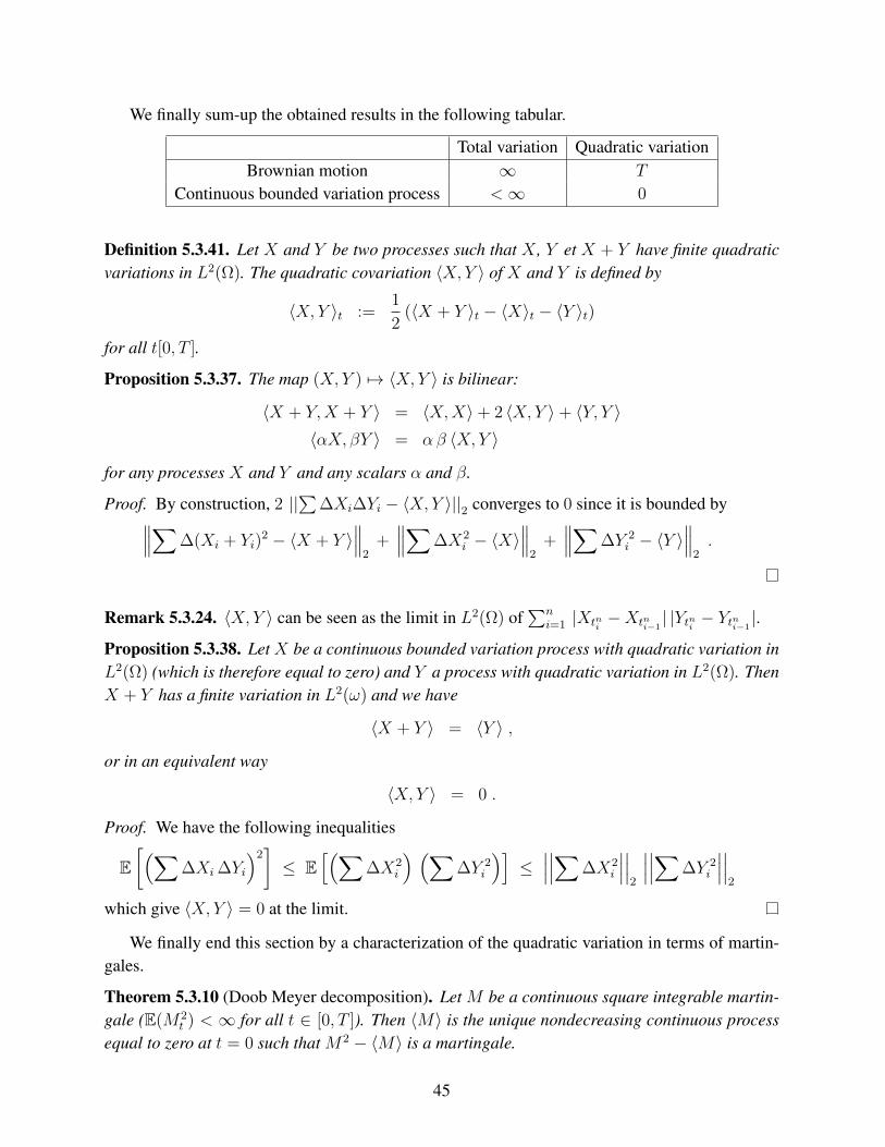
We finally sum-up the obtained results in the following tabular.

Total variation Quadratic variationBrownian motion ∞ T

Continuous bounded variation process <∞ 0

Definition 5.3.41. Let X and Y be two processes such that X , Y et X + Y have finite quadraticvariations in L2(Ω). The quadratic covariation 〈X, Y 〉 of X and Y is defined by

〈X, Y 〉t :=1

2(〈X + Y 〉t − 〈X〉t − 〈Y 〉t)

for all t[0, T ].

Proposition 5.3.37. The map (X, Y ) 7→ 〈X, Y 〉 is bilinear:

〈X + Y,X + Y 〉 = 〈X,X〉+ 2 〈X, Y 〉+ 〈Y, Y 〉〈αX, βY 〉 = αβ 〈X, Y 〉

for any processes X and Y and any scalars α and β.

Proof. By construction, 2 ||∑

∆Xi∆Yi − 〈X, Y 〉||2 converges to 0 since it is bounded by∥∥∥∑∆(Xi + Yi)2 − 〈X + Y 〉

∥∥∥2

+∥∥∥∑∆X2

i − 〈X〉∥∥∥

2+∥∥∥∑∆Y 2

i − 〈Y 〉∥∥∥

2.

Remark 5.3.24. 〈X, Y 〉 can be seen as the limit in L2(Ω) of∑n

i=1 |Xtni−Xtni−1

| |Ytni − Ytni−1|.

Proposition 5.3.38. Let X be a continuous bounded variation process with quadratic variation inL2(Ω) (which is therefore equal to zero) and Y a process with quadratic variation in L2(Ω). ThenX + Y has a finite variation in L2(ω) and we have

〈X + Y 〉 = 〈Y 〉 ,

or in an equivalent way

〈X, Y 〉 = 0 .

Proof. We have the following inequalities

E[(∑

∆Xi ∆Yi

)2]≤ E

[(∑∆X2

i

) (∑∆Y 2

i

)]≤∣∣∣∣∣∣∑∆X2

i

∣∣∣∣∣∣2

∣∣∣∣∣∣∑∆Y 2i

∣∣∣∣∣∣2

which give 〈X, Y 〉 = 0 at the limit.

We finally end this section by a characterization of the quadratic variation in terms of martin-gales.

Theorem 5.3.10 (Doob Meyer decomposition). Let M be a continuous square integrable martin-gale (E(M2

t ) < ∞ for all t ∈ [0, T ]). Then 〈M〉 is the unique nondecreasing continuous processequal to zero at t = 0 such that M2 − 〈M〉 is a martingale.

45

5.4 Stochastic integration

In this section we aim at defining an integral∫ T

0θs dBs w.r.t. the Brownian motion B for a class

of processes θ.For a regular function g and a differentiable function f , the integral of g w.r.t. f is defined by∫ T

0

g(s) df(s) =

∫ T

0

g(s) f ′(s)ds .

When f is not differentialble any more, this integral can be generalized to the case where f is afinite variation function as follow∫ T

0

g(s) df(s) = limπn→0

n−1∑i=0

g(ti)(f(tni+1)− f(tni )) (5.4.2)

where Πn = tn0 , . . . , tnn is a sudivision of [0, T ] for all n ≥ 1. This integral is called the Stieljesintegral.

In our case, we cannot use this definition of the integral since the Brownian motion is nota finite variation process.

To give a sense to the integral w.r.t. the Brownian motion we use the fact that it has finitequadratic variation. This leads us to work in an L2 type space. More precisely, we extend (5.4.2)by considering an L2 sense for the limit:∫ T

0

θs dBs = limπn→0

n−1∑i=0

θti(Bti+1−Bti)

Since we work with an L2 sense, we ask the process θ to be square integrable and also adapted. Wenow give the precise definition of the square integrability we need. We fix in the sequel a completeright-continuous1 filtration F = (Ft)t∈[0,T ]. We define the set L2

F(Ω, [0, T ]) by

L2F(Ω, [0, T ]) =

(θt)0≤t≤T F-adapted process s.t. θ ∈ L2(Ω, [0, T ])

We first construct the stochastic integral on a smaller set.

Definition 5.4.42. A process (θt)0≤t≤T is an elementary process if there exists a subdivision 0 =

t0 ≤ t1 ≤ . . . ≤ tn = T and a discrete time process (Θi)0≤i≤n−1 such that

– Θi is Fti-measurable for all i = 0, . . . , n− 1,

– Θi ∈ L2(Ω) for all i = 0, . . . , n− 1,

– The following identification

θt(ω) =n−1∑i=0

Θi(ω)1]ti,ti+1](t) (5.4.3)

holds for all t ∈ [0, T ].1i.e. ∩ε>0Ft+ε = Ft for all t ∈ [0, T ).

46

We denote by E2F(Ω, [0, T ]) the set of elementary processes. .

We notice that the set of elementary process is a subset of Ł2F(Ω, [0, T ]): E2

F(Ω, [0, T ]) ⊂Ł2F(Ω, [0, T ])

Definition 5.4.43. Let θ ∈ E2F(Ω, [0, T ]) satisfying the decomposition (5.4.3). The stochastic

integral between 0 and t ∈ [0, T ] of θ w.r.t. B is the random variable∫ t

0θsdBs defined by∫ t

0

θsdBs :=k∑i=0

Θi(Bti+1−Bti) + Θi(Bt −Btk) ,

where k is such that t ∈]tk, tk+1]. It can also be witten∫ t

0

θsdBs =n∑i=0

Θi(Bt∧ti+1−Bt∧ti) . (5.4.4)

To a process θ ∈ E2F(Ω, [0, T ]) we then associate the process

∫ .0θsdBs =

(∫ t0θsdBs

)t∈[0,T ]

.

Remark 5.4.25. According the Chasles relation we define∫ tsθu by∫ t

s

θu = dBu :=

∫ t

0

θudBu −∫ s

0

θudBu

for any s, t ∈ [0, T ].

Proposition 5.4.39. [Properties of the stochastic integral on E2F(Ω, [0, T ])]

(1) θ 7→∫ t

0θsdBs is a linear map on E2

F(Ω, [0, T ]).

(2) The process∫ .

0θsdBs is continuous for all θ ∈ E2

F(Ω, [0, T ]).

(3) The process∫ .

0θsdBs is F-adapted for all θ ∈ E2

F(Ω, [0, T ]).

(4) E[∫ t

0θsdBs

]= 0 and V ar

(∫ t0θsdBs

)= E

[∫ t0θ2sds]

for all θ ∈ E2F(Ω, [0, T ]).

(5) Isometry property:

E

[(∫ t

0

θsdBs

)2]

= E[∫ t

0

θ2sds

]for all θ ∈ E2

F(Ω, [0, T ]) and all t ∈ [0, T ].

(6) More generaly, we have

E[∫ t

s

θudBu|Fs]

= 0 et E

[(∫ t

s

θvdBv

)2

|Fs

]= E

[∫ t

s

θ2vdv|Fs

]for all θ ∈ E2

F(Ω, [0, T ]) and all s, t ∈ [0, T ] such that s ≤ t.

47

(7) We also have the general result

E[(∫ t

s

θvdBv

)(∫ u

s

φvdBv

)|Fs]

= E[∫ t∧u

s

θvφvdv|Fs]

for all θ, φ ∈ E2F(Ω, [0, T ]) and all t, s ∈ [0, T ].

(8) The process(∫ t

0θsdBs

)0≤t≤T

is an F-martingale for all θ ∈ E2F(Ω, [0, T ]).

(9) The process((∫ t

0θsdBs

)2

−∫ t

0θ2sds

)0≤t≤T

is an F-martingale for all θ ∈ E2F(Ω, [0, T ]).

(10) The quadratic variation of the stochastic integral is given by⟨∫ t

0

θsdBs

⟩=

∫ t

0

θ2sds

for all θ ∈ E2F(Ω, [0, T ]) and all t ∈ [0, T ].

(11) The quadratic covariation between two stochastic integrals given by⟨∫ t

0

θsdBs,

∫ u

0

φsdBs

⟩=

∫ t∧u

0

θsφsds

for all θ, φ ∈ E2F(Ω, [0, T ]) and all t, u ∈ [0, T ].

Proof. (1) The linearity is an immediate property.(2) The continuity of the stochastic integral is obtained from the second form (5.4.4) of the stochas-tic integral and the continuity of the Brownian motion.(3) For θ ∈ E2

F(Ω, [0, T ]) with decomposition as in (5.4.3) and t ∈ [0, T ], the random variable∫ t0θsdBs is Ft-measurable as the sum somme of Ft-measurable random variables. The stochastic

integral is therefore an F-adapted process.(4) Fix θ ∈ E2

F(Ω, [0, T ]) with decomposition as in (5.4.3). Without loss of generality, we canassume that t = tk . We then have from Proposition 1.3.8 (i) and (ii) and Proposition 1.3.9

E[∫ t

0

θsdBs

]=

k−1∑i=0

E[Θi(Bti+1

−Bti)]

=k−1∑i=0

E[ΘiE

[Bti+1

−Bti |Fti]]

= 0 .

48

For the variance we have by the same arguments

V ar

(∫ t

0

θsdBs

)= E

[(∫ t

0

θsdBs

)2]

= E

(k−1∑i=0

Θi(Bti+1−Bti)

)2

=k−1∑i=0

E[Θ2i (Bti+1

−Bti)2]

+ 2∑i<j

E[Θi Θj(Bti+1

−Bti) (Btj+1−Btj)

]=

k−1∑i=0

Θ2iE[(Bti+1

−Bti)2|Fti

]+ 2

∑i<j

E[Θi Θj(Bti+1

−Bti)E[Btj+1−Btj |Ftj ]

]=

k−1∑i=0

Θ2i (ti+1 − ti) + 0 =

∫ t

0

θ2sds

(5) The isometry property comes from the previous computations of the expectation and the vari-ance.(6) Fix s, t ∈ [0, T ] s.t. s ≤ t and θ ∈ E2

F(Ω, [0, T ]) with decomposition as in (5.4.3). We canassume w.l.o.g. that s = tj et t = tk for some j, k ≤ n. We then have

E[∫ t

0

θudBu|Fs]

= E

[k−1∑i=0

Θi(Bti+1−Bti)|Ftj

]

= E

[j−1∑i=0

Θi(Bti+1−Bti)|Ftj

]+

k−1∑i=j

E[Θi(Bti+1

−Bti)|Ftj]

=

j−1∑i=0

Θi(Bti+1−Bti) +

k−1∑i=j

E[

Θi E[Bti+1−Bti |Fti ] |Ftj

]=

∫ s

0

θudBu + 0 .

49

For the second order moment we have

E

[(∫ t

s

θudBu

)2

|Fs

]

= E

(k−1∑i=j

Θi(Bti+1−Bti)

)2

|Ftj

=

k−1∑i=j

E[Θ2i (Bti+1

−Bti)2|Ftj

]+ 2

∑i<l

E[Θi Θl(Bti+1

−Bti) (Btl+1−Btl)|Ftj

]=

k−1∑i=j

E[Θ2iE[(Bti+1

−Bti)2|Fti

]|Ftj

]+ 2

∑i<l

E[Θi Θl(Bti+1

−Bti)E[Btl+1−Btl |Ftl ]|Ftj

]=

k−1∑i=j

E[Θ2i (ti+1 − ti)|Ftj

]+ 0

= E[∫ t

s

θ2udu|Fs

].

(7) For θ, φ ∈ E2F(Ω, [0, T ]) and u ≤ t we have

2E[(∫ t

s

θvdBv

)(∫ u

s

φvdBv

)|Fs]

= E

[(∫ t

s

(θv + φv1v≤u)dBv

)2

|Fs

]− E

[(∫ t

s

θvdBv

)2

|Fs

]− E

[(∫ u

s

φvdBv

)2

|Fs

]

= E[∫ t

s

(θv + φv1v≤u)2dv|Fs

]− E

[∫ t

s

θ2vdv|Fs

]− E

[∫ u

s

φ2vdv|Fs

]= 2E

[∫ u

s

θvφvdv|Fs]

(8) We have seen that the process∫ .

0θsdBs is F-adapted. From the isometry property, we get that

this process is square integrable and hence integrable. The first part of the property (6) gives theconditional property of martingales.

(9) The process M =

((∫ t0θsdBs

)2

−∫ t

0θ2sds

)0≤t≤T

is F-adapted as the sum of F-adapted

dicrete time processes. M is also integrable as the sum of two integrable processes. The secondpart of the property (6) gives the martingale property of M .(10) From Theorem 5.3.10 and point (9) we get point (10).(11) The result comesfrom the definition of the covariation and the same computation as in (8).

Example: We have ∫ t

0

dBs = Bt −B0 = Bt

50

for all t ∈ [0, T ].

We notice that the stochastic integral of a process in E2F(Ω, [0, T ]) is a square integrable F-

martingale. We therefore define the setM2([0, T ]) by

M2([0, T ]) :=M F-martingale such that E[M2

t ] <∞ for all t ∈ [0, T ]

As defined now, the stochastic integration is a linear map from E2F(Ω, [0, T ]) toM2([0, T ]). We

now extend the stochastic integration to L2F(Ω, [0, T ]). To this end we need the following lemma.

Lemma 5.4.1. The set of elementary processes E2F(Ω, [0, T ]) is dense in L2

F(Ω, [0, T ]) for the norm‖ · ‖′2. In other words, for any θ ∈ L2

F(Ω, [0, T ]), there exists a sequence (θn)n in E2F(Ω, [0, T ])

such that

‖θn − θ‖′2 = E[∫ T

0

(θs − θns )2 ds

]1/2

−→ 0 as n → ∞ .

We admit this Lemma. The extension of the stochastic integral is given by the following result.

Theorem 5.4.11. There exists a unique linear map I from L2F(Ω, [0, T ]) to M2([0, T ]) which

coincides with the stochastic integral on E2F(Ω, [0, T ]) and satisfies the isometry property:

E[I(θ)2

t

]= E

[∫ t

0

θ2s ds

]for all θ ∈ L2

F(Ω, [0, T ]) and all t ∈ [0, T ].

Proof. Approximation: Fix θ ∈ L2F(Ω, [0, T ]). From the previous Lemma, There exists a se-

quence (θn)n in E2F(Ω, [0, T ]) such that

‖θ − θn‖′2 = E[∫ T

0

(θs − θns )2 ds

]1/2

−→ 0 .

Convergence: From the isometry property between 0 and t ∈ [0, T ] applied to the process (θn+p −θn) ∈ E2

F(Ω, [0, T ]) we have

E

[(∫ t

0

(θn+ps − θns )dBs

)2]

= E[∫ t

0

(θn+ps − θns )2ds

]≤ E

[∫ T

0

(θn+ps − θns )2ds

],

which can be rewrtitten∥∥∥∥∫ t

0

θn+ps dBs −

∫ t

0

θns dBs

∥∥∥∥2

≤∥∥θn+p − θn

∥∥′2. (5.4.5)

Since (θn)n converges in L2(Ω, [0, T ]), it is a Cauchy sequence. From (5.4.5), the sequence(∫ t

0θns dBs)n is Cauchy in L2(Ω). L2(Ω) endowed with ‖.‖2 being a Banach space, the sequence

51

(∫ t

0θns dBs) converges in L2(Ω). If we denote by

∫ t0θsdBs its limit, we get by sending p to infinity

in (5.4.5)

E

[(∫ t

0

θs dBs −∫ t

0

θns dBs

)2]

= E[∫ t

0

(θs − θns )2ds

].

Uniqueness: Suppose that (θn)n et (φn)n are two approximating sequences in E2F(Ω, [0, T ]) for

θ ∈ L2F(Ω, [0, T ]). From the isometry property, we have∥∥∥∥∫ t

0

θns dBs −∫ t

0

φnsdBs

∥∥∥∥2

= E[∫ t

0

(θns − φns )2ds

]1/2

≤ ‖θn − φn‖′2

Therefore, by sending n to infinity we get that∫ t

0θns dBs −

∫ t0φnsdBs in L2(Ω).

Convergence inM2([0, T ]): Since for each t ∈ [0, T ],∫ t

0θsdBs is the limit in L2(Ω) of

∫ t0θns dBs

with θn ∈ E2F(Ω, [0, T ]), we get from Proposition 5.1.30 with p = 2 that the limit process

∫ .0θsdBs

belongs toM2([0, T ]).

Linarity and Isometry: The linearity of I is obvious. Using the isometry property on E2F(Ω, [0, T ])

we have

E

[(∫ t

0

θns dBs

)2]

= E[∫ t

0

(θns )2ds

].

Sending n to infinity we get

E

[(∫ t

0

θsdBs

)2]

= E[∫ t

0

θ2sds

].

We now extend the properties of the stochastic integral to Ł2F(Ω, [0, T ]).

Proposition 5.4.40. [Properties of the stochastic integral on L2F(Ω, [0, T ])]

(1) θ 7→∫ t

0θsdBs is a linear map on L2

F(Ω, [0, T ]).

(2) The process∫ .

0θsdBs is continuous for all θ ∈ L2

F(Ω, [0, T ]).

(3) The process∫ .

0θsdBs is F-adapted for all θ ∈ L2

F(Ω, [0, T ]).

(4) E[∫ t

0θsdBs

]= 0 and V ar

(∫ t0θsdBs

)= E

[∫ t0θ2sds]

for all θ ∈ L2F(Ω, [0, T ]).

(5) Isometry property:

E

[(∫ t

0

θsdBs

)2]

= E[∫ t

0

θ2sds

]for all θ ∈ Ł2

F(Ω, [0, T ]) and all t ∈ [0, T ].

52

(6) More generaly, we have

E[∫ t

s

θudBu|Fs]

= 0 et E

[(∫ t

s

θvdBv

)2

|Fs

]= E

[∫ t

s

θ2vdv|Fs

]for all θ ∈ Ł2

F(Ω, [0, T ]) and all s, t ∈ [0, T ] such that s ≤ t.

(7) We also have the general result

E[(∫ t

s

θvdBv

)(∫ u

s

φvdBv

)|Fs]

= E[∫ t∧u

s

θvφvdv|Fs]

for all θ, φ ∈ L2F(Ω, [0, T ]) and all t, s ∈ [0, T ].

(8) The process(∫ t

0θsdBs

)0≤t≤T

is an F-martingale for all θ ∈ Ł2F(Ω, [0, T ]).

(9) The process((∫ t

0θsdBs

)2

−∫ t

0θ2sds

)0≤t≤T

is an F-martingale for all θ ∈ L2F(Ω, [0, T ]).

(10) The quadratic variation of the stochastic integral is given by⟨∫ t

0

θsdBs

⟩=

∫ t

0

θ2sds

for all θ ∈ L2F(Ω, [0, T ]) and all t ∈ [0, T ].

(11) The quadratic covariation between two stochastic integrals given by⟨∫ t

0

θsdBs,

∫ u

0

φsdBs

⟩=

∫ t∧u

0

θsφsds

for all θ, φ ∈ L2F(Ω, [0, T ]) and all t, u ∈ [0, T ].

Proof. We have already proved (1) (3), (5) and (8).(2)The isomtry property give the continuity in L2(Ω). We admit the P-a.s. continuity.(4) is a particular case of (6).(6) The first equality is the martingale property of the stochastic integral and the second equalityis the martingale property of the the process given by (9).(7) We get it from (6) as in E2

F(Ω, [0, T ]) by considering θ2, φ2 and (θ + φ)2.(9) We obtain it by the Proposition (5.1.30) with p = 1.(10) is given by Theorem 5.3.10.(11) is a direct consequence of (10).

Remark 5.4.26. Since the stochastic integral is defined as a limit in L2(Ω) it is defined up to aP-a.s. modification.

53

The case of deterministic process θ.

Proposition 5.4.41. Suppose that the process θ is a deterministic function f of the time variable.Then the stochastic integral

∫ t0f(s)dBs is au Gaussian random variable called the Wiener inte-

gral with law given by ∫ t

0

f(s)dBs ∼ N(

0,

∫ t

0

f 2(s)ds

).

Proof. Indeed,∫ t

0f(s)dBs can be written as the limit in L2(Ω) of random variables of the form

n−1∑i=0

f(tni )(Btni+1−Btni

)

where tni = int for i = 1, . . . , n and n ≥ 1. We notice that

∑n−1i=0 f(tni )(Btni+1

− Btni) As a limit

in L2(Ω) of Gaussian random variable,∫ t

0f(s)dBs is also a Gaussian random variable Since the

convergence in L2(Ω) implies the convergence and the expectation and the variance we get

E[ ∫ t

0

f(s)dBs

]= 0 and V ar

[ ∫ t

0

f(s)dBs

]=

∫ t

0

f 2(s)ds .

Moreover, any linear combination of the∫ ti

0f(s)dBs is also a Wiener integral and hence a

Gaussian random variable. Therefore the process∫ .

0f(s)dBs is a Gaussian process with covari-

ance function given by

Cov

(∫ t

0

f(s)dBs,

∫ u

0

g(s)dBs

)=

∫ t∧u

0

f(s)g(s)ds .

We can also prove that the random variable∫ tsf(u)dBu is independent of σ(Bu : u ≤ s).

The case where the process θ is a deterministic function f(B) of the Brownian motion.We have seen that for a sequence (θn) in E2

F(Ω, [0, T ]) converging to θ in L2(Ω, [0, T ]), thestochastique integral

∫θdB is the limit in L2(Ω) of the sequence (

∫θndB)n. In the case where

theta is of the form f(B). A natural sequence to approach the stochastic integral∫ T

0f(B)dB is

the followingn−1∑i=0

f(Btni)(Btni+1

−Btni)

where tni = inT for i = 1, . . . , n and n ≥ 1. We study the conditions under which we have

convergence.

Proposition 5.4.42. Suppose that the function f admits a bounded first order derivative. Then wehave then following convergence in L2(Ω):

n−1∑i=0

f(B inT )(B (i+1)

nT−B i

nT )

L2

−→∫ T

0

f(Bs)dBs as n→∞.

54

Proof. First, we have to prove that the stochastic integral is well defined under these conditionsi.e. f(B) ∈ L2

F(Ω, [0, T ]). The process f(B) is F-adapted since B is an F-Brownian motion.Morevoer we have

|f(Bt)| ≤ |f(B0)| + ‖f ′‖∞.|Bt −B0| = |f(0)| + ‖f ′‖∞.|Bt|

The constant |f(0)| belongs to L2F(Ω, [0, T ]) and we have

E[∫ T

0

|Bs|2ds]

=

∫ T

0

E[|Bs|2] ds =

∫ T

0

s ds =T 2

2< ∞

Therefore f(Bt) ∈ L2F(Ω, [0, T ]) and

∫ T0f(Bs)dBs is well defined.

For n ≥ 1, define the process Bn by

Bnt :=

n−1∑i=0

Btni1]tni ,t

ni+1](t)

for all t ∈ [0, T ]. Then we have∫ T

0

f(Bns ) dBs :=

n−1∑i=0

f(B inT )(B (i+1)

nT−B i

nT )

We then have

‖f(B)− f(Bn)‖′2 = E[∫ T

0

(f(Bs)− f(Bns ))2 ds

]1/2

= E

[n−1∑i=0

∫ ti+1

ti

(f(Bs)− f(Bti))2 ds

]1/2

≤ ‖f ′‖∞

(n−1∑i=0

∫ ti+1

ti

E[(Bs −Bti)2] ds

)1/2

= ‖f ′‖∞

(n−1∑i=0

∫ ti+1

ti

(s− ti) ds

)1/2

= ‖f ′‖∞

(n

∫ T/n

0

u du

)1/2

=T‖f ′‖∞

2√n

−→n→∞

0 .

Therefore f(Bn)converges in L2(Ω, [0, T ]) to f(B). We then deduce that∫ T

0f(Bn

s )dBs convrgesto∫ T

0f(Bs)dBs in L2(Ω).

Example: how to compute∫ T

0Bs dBs ?

55

Using the processBn. :=

∑n−1i=0 Bti1]ti,ti+1](.), The previous Proposition gives the convergence

in L2(Ω) of∫ T

0Bns dBs to

∫ T0Bs dBs. We then notice that

2

∫ T

0

Bns dBs = 2

n−1∑i=0

Bti(Bti+1−Bti) ds =

n−1∑i=0

(B2ti+1−B2

ti) −

n−1∑i=0

(Bti+1−Bti)

2

= B2T +

n−1∑i=0

(Bti+1−Bti)

2

The second term in the r.h.s converges in L2(Ω) to the quadratic variation of B on [0, T ]. Wefinally get

B2T =

∫ T

0

2Bs dBs + T .

We retreive the fact that (B2t − t)t≥0 is a martingale. The additional term comes from the quadratic

variation of B.Loosely speaking, one can say that a small variation dBt of B corresponds to a variation

√dt

since its quadratic variation is dt i.e.

dBt ∼√dt ⇒ (dBt)

2 ∼ dt

5.5 Ito’s formula

We introduce the main skill to compute stochastic integrals without using approximation se-quences of E2

F(Ω, [0, T ]).

Theorem 5.5.12. Let f ∈ C2(R) with bounded second order derivative. We then have

f(Bt) = f(B0) +

∫ t

0

f ′(Bs) dBs +1

2

∫ t

0

f ′′(Bs) ds

for all t ∈ [0, T ]. The infinitesimal notation of this formula is

d f(Bs) = f ′(Bs) dBs +1

2f ′′(Bs) ds .

Proof. Fix t ∈ [0, T ] and consider the subdivision t0 < t1 < · · · < tn of the interval [0, t] withti = it/n. From Taylor formula and the continuity ofB we have

f(Bt) − f(B0) =n∑i=1

[f(Bti)− f(Bti−1)]

=n∑i=1

f ′(Bti)(Bti −Bti−1) +

1

2

n∑i=1

f ′′(Bθi)(Bti −Bti−1)2

56

where θi is a random time valued in ]ti−1, ti[ for each i = 1, . . . , n. Since f ′ is differentiable withbounded derivative, we have from Proposition 5.4.42∥∥∥∥∥

n∑i=1

f ′(Bti)(Bti −Bti−1) −

∫ t

0

f ′(Bs) dBs

∥∥∥∥∥2

−→n→∞

0

We now study the term

Un :=n∑i=1

f ′′(Bθi)(Bti −Bti−1)2

We aim at replacing θi by ti−1 in a first time and (Bti − Bti−1)2 by ti − ti−1 in a second time.

Define the sequences (Vn)n and (Wn)n by

Vn :=n∑i=1

f ′′(Bti−1)(Bti −Bti−1

)2 et Wn :=n∑i=1

f ′′(Bti−1)(ti − ti−1)

From Cauchy-Schwartz inequality we have

E[|Un − Vn|] ≤ E

[supi|f ′′(Bti−1

)− f ′′(Bθi)|n∑i=1

(Bti −Bti−1)2

]

≤ E[supi|f ′′(Bti−1

)− f ′′(Bθi)|2]1/2

E

( n∑i=1

(Bti −Bti−1)2

)21/2

E

[sup

u,s≤t , |u−s|≤ tn

|f ′′(Bs)− f ′′(Bu)|2]1/2

E

( n∑i=1

(Bti −Bti−1)2

)21/2

The function s 7→ f ′′(Bs) is P-a.s. continuous on the compact [0, t], hence it is P-a.s. uniformlycontinuous on [0, t]. Since f ′′ is bounded, we get from Lebesgue dominated convergence theoremthat

E

[sup

u,s≤t , |u−s|≤ tn

|f ′′(Bs)− f ′′(Bu)|2]−→n→∞

0 .

For the second term we have from the definition of quadratic variation

E

( n∑i=1

(Bti −Bti−1)2

)21/2

−→n→∞

t .

57

We therefore deduce that a ‖Un − Vn‖1 → 0. We now study the difference Vn −Wn. We have

E[|Vn −Wn|2] = E

( n∑i=1

f ′′(Bti−1)((Bti −Bti−1

)2 − (ti − ti−1))

)2

=n∑i=1

E[(f ′′(Bti−1

)((Bti −Bti−1)2 − (ti − ti−1))

)2]

≤ ‖f ′′‖2∞

n∑i=1

V ar((Bti −Bti−1)2)

= ‖f ′′‖2∞

n∑i=1

2(ti − ti−1)2 = 2 ‖f ′′‖2∞t2

n−→n→∞

0

We deduce ‖Vn −Wn‖2 −→n→∞

0. Finally, from the definition of the Lebesgue intgral and since f ′′

is bounded, we have ∥∥∥∥Wn −∫ t

0

f ′′(Bs)ds

∥∥∥∥1

−→n→∞

0

The convergence in L2(Ω) being stronger than the convergence in L1(Ω), we finaly get

f(Bt) − f(B0) =n∑i=1

f ′(Bti)(Bti −Bti−1) +

1

2

n∑i=1

f ′′(Bθi)(Bti −Bti−1)2

−→n→∞

∫ t

0

f ′(Bs) dBs +1

2

∫ t

0

f ′′(Bs) ds

in L1(Ω), which implies the P-a.s. equality between these two random variables.

Example: We retrieve BT =∫ T

0dBt et B2

T = 2∫ T

0BsdBs + T

Extension to the case of unbounded second order derivativeThe assumption that f ′′ is bounded is restrictive and prevent us from applying Ito’s formula to

simplest financial models.Actually, we can extend the definition of the stochastic integral w.r.t. B to the setL2

F ,loc(Ω, [0, T ])

including L2F(Ω, [0, T ]) and defined by

L2F ,loc(Ω, [0, T ]) :=

(θs)0≤s≤T B([0, T ])⊗A-measurable process and

F-adapted s.t.∫ T

0

|θs|2ds <∞ P− a.s.

By this generalisation, the martingale property of the stochastic integral is lost. It is replacedby a local martingale property. The Ito’s formula can the be generalised as follows.

58

Theorem 5.5.13. For any function f ∈ C2(R) we have

f(Bt) = f(B0) +

∫ t

0

f ′(Bs) dBs +1

2

∫ t

0

f ′′(Bs) ds , P− a.s.

for all t ∈ [0, T ].

We notice that in the previous formula, the stochastic integral appearing in the l.h.s. is welldefined even if f ′′ is not bounded, thanks to the extension to L2

F ,loc(Ω, [0, T ]) of the stochasticintegration.

5.6 Ito’s processes

We introduce a new class of process with respect to which we can extend the stochastic integration.

Definition 5.6.44. An Ito process is a process of the form

Xt = X0 +

∫ t

0

ϕs ds +

∫ t

0

θs dBs (5.6.6)

with X0 F0-measurable, θ and ϕ two F-adapted processes satisfying the integrability condition∫ T

0

|θs|2ds <∞ a.s. and∫ T

0

|ϕs|ds <∞ a.s.

We also write

dXt = ϕt dt + θt dBt

To be able to prove results on this class of processes, we need to impose the stronger integra-bility condition on θ and ϕ

(CI) E[∫ T

0

|θs|2ds]<∞ and E

[∫ T0|ϕs|2ds

]<∞ .

Proposition 5.6.43. Let M be a continuous martingale such that Mt :=∫ t

0ϕsds for t ∈ [0, T ]

with ϕ ∈ L2F(Ω, [0, T ]). Then we have

Mt = 0

for all t ∈ [0, T ].

Proof. By definition M0 = 0 and since M is a martingale we have

E[M2t ] = E

( n∑i=1

M itn−M (i−1)t

n

)2

= E

[n∑i=1

(M it

n−M (i−1)t

n

)2]

= E

n∑i=1

(∫ itn

(i−1)tn

ϕsds

)2 .

59

From Cauchy-Schwartz inequality we have(∫ itn

(i−1)tn

ϕsds

)2

≤∫ it

n

(i−1)tn

12ds

∫ itn

(i−1)tn

ϕ2sds =

t

n

∫ itn

(i−1)tn

ϕ2sds

Taking the sum of these terms over i = 1, . . . , n we get

E[M2t ] ≤ E

[n∑i=1

t

n

∫ itn

(i−1)tn

ϕ2sds

]=

t

nE[∫ t

0

ϕ2sds

]−→n→∞

0 .

We then deduce that P-a.s. Mt = 0.

Corollary 5.6.1. The decomposition (5.6.6) of an Ito process X with θ and ϕ satisfying condition(CI) is unique.

Proof. Suppose that an Ito process has two decompositions:

Xt = X0 +

∫ t

0

ϕ1s ds +

∫ t

0

θ1s dBs = X0 +

∫ t

0

ϕ2s ds +

∫ t

0

θ2s dBs

for all t ∈ [0, T ]. Then we have∫ t

0

(ϕ1s − ϕ2

s) ds =

∫ t

0

(θ2s − θ1

s) dBs

for all t ∈ [0, T ]. The r.h.s. is a continuous martingale continue which can be written as an integralw.r.t. the Lebesgue measure. We get from Proposition 5.6.43 that∫ t

0

(ϕ1s − ϕ2

s) ds =

∫ t

0

(θ2s − θ1

s) dBs = 0 .

for all t ∈ [0, T ]. From that we first deduce that ϕ1 = ϕ2. Moreover, using the isometry propertywe get

E[∫ t

0

(θ2s − θ1

s)2 ds

]= E

[∫ t

0

(θ2s − θ1

s) dBs

]= E[0] = 0

for all t ∈ [0, T ], which gives θ2 = θ1.

Corollary 5.6.2. Let X be an Ito process with decomposition (5.6.6) satisfying condition (CI).Then X is a martingale if and only if the process ϕ is equal to zero.

Proof. If the process ϕ is equal to zero, then X is the stochastic integral of θ ∈ L2F(ω, [0, T ]).

Thus, it is a martingales.Consider now an Ito process X given by (5.6.6), satisfying (CI), which is a martingale. Then

the process (Xt − X0 −∫ t

0θs dBs)t∈[0,T ] is a continuous martingale of the form (

∫ t0ϕs ds)t∈[0,T ]

with ϕ ∈ L2F(Ω, [0, T ]). From Proposition 5.6.43 we get that

∫ t0ϕs ds = 0 for all t ∈ [0, T ] and

therefore ϕ = 0.

60

These results can be generalized to the case where θand ϕ does not satisfy (CI).

Proposition 5.6.44. 1. If M is a continuous local martingale of the form Mt :=∫ t

0ϕsds with

ϕ satisfying∫ T

0|ϕs|ds <∞ P-a.s. then

Mt = 0

for all t ∈ [0, T ].

2. The decompositions of an Ito process is unique.

3. An Ito process is a local martingale if and only if its term ϕ is equal to zero.

We now study the quadratic variation of an Ito process.

Proposition 5.6.45. The quadratic variation of an Ito process X with decomposition (5.6.6) isgiven by

〈X〉t =

⟨∫ .

0

θs dBs

⟩t

=

∫ t

0

θ2s ds

for all t ∈ [0, T ].

Proposition 5.6.46. The quadratic covariation between two Ito processes X1 et X2 with decom-position

dX it = ϕit dt + θit dBt

is given by

〈X1, X2〉t =

∫ t

0

θ1s θ

2s ds

Proof. By definition, the quadratic covariation is given by

〈X1, X2〉t :=1

2

(〈X1 +X2〉t − 〈X1〉t − 〈X2〉t

)=

1

2

(∫ t

0

(θ1s + θ2

s)2 ds −

∫ t

0

(θ1s)

2 ds −∫ t

0

(θ2s)

2 ds

)=

∫ t

0

θ1s θ

2s ds

Definition 5.6.45. Let X be an Ito process given by (5.6.6) with θ and ϕ satifying condition (CI).For process φ ∈ L2

F(Ω, [0, T ]) satisfying

E[ ∫ T

0

|φsϕs|ds]< ∞

61

and

E[ ∫ T

0

|φsθs|2ds]< ∞ .

For t ∈ [0, T ], we define the stochastic integral of φ w.r.t. X on [0, t] by∫ t

0

φs dXs :=

∫ t

0

φs θs dBs +

∫ t

0

φs ϕs ds

The Ito formula can also be generalized to Ito processes as follows.

Theorem 5.6.14. Let f be a C2 function. Then we have

f(Xt) = f(X0) +

∫ t

0

f ′(Xs) dXs +1

2

∫ t

0

f ′′(Xs) d〈X〉s

= f(X0) +

∫ t

0

f ′(Xs)ϕs ds +

∫ t

0

f ′(Xs)θs dBs +1

2

∫ t

0

f ′′(Xs) θ2sds

for all t ∈ [0, T ]. The infinitesimal notation of this relation is given by

df(Xt) = f ′(Xt) dXt +1

2f ′′(Xt) d〈X〉t

Proof. The proof consists in a Taylor development as in the case of the Brownian motion:

f(Xt) − f(X0) =n∑i=1

f ′(Xti)(Xti −Xti−1) +

1

2

n∑i=1

f ′′(Xθi)(Xti −Xti−1)2

The first term in the r.h.s. converges to the stochastic integral∫ t

0f ′(Xs) dXs and the second one

converges to 12

∫ t0f ′′(Xs) d〈X〉s by definition of the quadratic variation.

We notice that since X and f ′ are continuous, we have f ′(X)θ ∈ L2F ,loc(Ω, [0, T ]) and thanks

to the extension of the stochastic integral to L2F ,loc(Ω, [0, T ]) the term

∫ t0f ′(Xs)θsdBs is well

defined.

A direct implication of the Ito formula is the stochastic integration by part formula.

Proposition 5.6.47 (Stochastic integration by part formula). Let X and Y be two Ito processes.Then we have

XtYt = X0Y0 +

∫ t

0

XsdYs +

∫ t

0

YsdXs +

∫ t

0

d〈X, Y 〉s

for all t ∈ [0, T ]. The infinitesimal notation for this formula is given by

d(XY )t = XtdYt + YtdXt + d〈X, Y 〉t

62

Proof. Applying Ito’s formula to X2t et Y 2

t , we have

dX2t = 2XtdXt +

2

2d〈X〉t and dY 2

t = 2YtdYt +2

2d〈Y 〉t

Applying Ito’s formula to (X + Y )2, we get

d(X + Y )2t = 2(Xt + Yt)d(Xt + Yt) +

2

2d〈X + Y 〉t

This gives

d(XY )t =1

2

(d(X + Y )2

t − dX2t − dY 2

t

)= XtdYt + YtdXt +

1

2(d〈X + Y 〉t − d〈X〉t − d〈Y 〉t)

= XtdYt + YtdXt + d〈X, Y 〉t

Different forms for Ito’s formula1. For the Brownian motion with f ∈ C2(R):

f(Wt) = f(W0) +

∫ t

0

f ′(Ws) dWs +1

2

∫ t

0

f ′′(Ws) ds

2. For an Ito process with f ∈ C2(R):

f(Xt) = f(X0) +

∫ t

0

f ′(Xs) dXs +1

2

∫ t

0

f ′′(Xs) d〈X〉s

3. For an Ito process with f ∈ C1,2([0, T ]× R)

f(t,Xt) = f(0, X0) +

∫ t

0

∂f

∂t(s,Xs) ds +

∫ t

0

∂f

∂x(s,Xs) dXs +

1

2

∫ t

0

∂2f

∂x2(s,Xs) d〈X〉s

4. For a multi-dimensional Ito process with f ∈ C1,2([0, T ]× Rd):

f(Xt) = f(X0) +d∑i=1

∫ t

0

∂f

∂xi(Xs) dXi(s) +

1

2

d∑i=1

d∑j=1

∫ t

0

∂2f

∂xi∂xj(Xs) d〈Xi, Xj〉s

5.7 Stochastic differential equation

As we define the notion of ordinary differential equation in the deterministic case, we define herean object called Stochastic Differential Equation (SDE for short). To this end we consider twomeasurable functions µ and σ from [0, T ]× R into R.

The SDE with drift µ and volatility σ is then given by an initial condition and a dynamics asfollows

X0 = x , dXt = µ(t,Xt)dt + σ(t,Xt)dWt t ∈ [0, T ]. (5.7.7)

We now give the precise definition of a solution to the SDE.

63

Definition 5.7.46. A process X is a solution to the SDE (5.7.7) if it is an F-adapted process andsatisfies ∫ T

0

|µ(s,Xs)|ds +

∫ T

0

σ2(s,Xs)ds < ∞ P− a.s

and

Xt = x +

∫ t

0

µ(s,Xs)ds +

∫ t

0

σ(s,Xs)dWs P− a.s.

for all t ∈ [0, T ].

These equations does not necessary have solutions. To ensure the existence and uniqueness ofsolution, we need two types of conditions.

The first one ensures the uniqueness through the Lipschitz propoerty of the functions µ et σ:

Condition 1: There exists a constant L > 0 such that

|µ(t, x)− µ(t, y)| + |σ(t, x)− σ(t, y)| ≤ L |x− y|

for all (t, x, y) ∈ R+ × R2.

The second condition garente that the process does not explode on the time intervall [0, T ].

Condition 2: There exists a constant M > 0 such that

|µ(t, x)|2 + |σ(t, x)|2 ≤ M (1 + |x|2)

for all (t, x) ∈ [0, T ]× R.

Theorem 5.7.15. Suppose that µ and σ satisfy Condition 1 and Condition 2. Then SDE (5.7.7)admits a unique solution.

This result is admitted. As for the deterministic case, the proof of this theorem is based on afixed point argument.

Remark 5.7.27. In the particular case where µ and σ do not depend on the variable t, Condition2 is implied by Condition 1 .

5.8 Exercices

5.8.1 Brownian bridge

Let (Bt)t∈[0,T ] be a Brownian motion. We define the process (Zt)t∈[0,1] by

Zt = Bt − tB1 , t ∈ [0, 1] .

64

1. Prove that (Zt)t∈[0,1] is a Gaussien process independent of B1.

2. Calculate the mean functionmt and the covariance functionK(Zs, Zt) of the process (Zt)t∈[0,1].

3. Prove that the process Z defined by

Zt = Z1−t , t ∈ [0, T ]

has the same law as Z.

5.8.2 SDE with affine coefficients

We consider the following SDE

Xt =

∫ t

0

(µXr + µ′)dr +

∫ t

0

(σXr + σ′)dBr , t ∈ [0, T ] .

We set St = exp((µ− σ2/2)t+ σBt

), t ∈ [0, T ].

1. Give the SDE satisfied by 1S

.

2. Prove that

d(Xt

St

)=

1

St

((µ′ − σσ′)dt+ σ′dBt

), t ∈ [0, T ] .

3. Deduce the expression of the process X .

5.8.3 Ornstein-Ulhenbeck process.

The Ornstein-Ulhenbeck process is the unique solution of the following SDEX0 given random variable ,

dXt = −cXtdt+ σdBt , t ∈ [0, T ] .(5.8.8)

We suppose that X0 is a Gaussian random variable independent of B.

1. Define the process Y by

Yt = Xt exp(ct) , t ∈ [0, T ] .

Give the SDE satisfied by Y . Deduce the expression of the process Y .

2. Deduce the expression of the process X

3. Give the law of the random variable Xt for t ∈ [0, T ]. Calculate cov(Xs, Xt) for t, s ∈ [0, T ].

4. Find the law for X0 such that the process X is stationary i.e. Xt and Xs have the same law forany s, t ∈ [0, T ].

5. What is the limit law of Xt when t goes to +∞?

65

Chapter 6

Black & Scholes Model

The first model for the evolution of financial assets was proposed by Louis Bachelier in his thesisin 1900. the assets were supposed to be Gaussian random variables. They could unfortunately takenegative values. To overcome this problem, a log-normal model was considered for the financialassets to ensure that they take positive values. This model is called the Black & Scholes model.

6.1 Assumptions on the market

We use the same assumptions as those presented in Chapter 2. We recall them for the convenienceof the reader.

– The assets are infinitely divisible: One can sell or buy an proportion of asset.

– Liquidity of the market: one can sell or buy any quantity of assets at any time.

– One can short sell any asset.

– There is no transaction costs.

– One can borrow and lend at the same interest rate r.

6.2 Probabilistic model for the market

To model the uncertainty of financial market, we consider a complete probability space (Ω,A,P)

endowed with a Brownian motion W . We suppose that the market is composed by a riskless assetS0 and a risky asset S defined on the time interval [0, T ].

• The riskless asset. We suppose that the riskless asset S0 starts from an initial value S0 = 1 andevolves according to the interest rate r time unit. Its is then given by

dS0t = rS0

t dt and S00 = 1 ⇒ S0

t = ert t ∈ [0, T ] .

66

• The risky asset. We suppose that the risky asset S is given by the SDEdSt = St (µ dt + σ dWt) , t ∈ [0, T ]

S0 = s0(6.2.1)

where µ and σ are two constants such that σ > 0.

This model is the simplest one that one can define to represent the evolution of a risky assetthat is constrained to be positive. As we will bellow, this leads to Gaussian asset yields .

For any t ∈ [0, T ], the σ-algebra Ft represents all the information available on the market attime t. The randomness is only given by the process S, thus we have

Ft := σ(Sr, r ≤ t)

for all t ∈ [0, T ]. The probability measure P is called the historical probability.

To ensure that this model is well posed, we need to solve the Black & Scholes SDE.

Theorem 6.2.16. The SDE (6.2.1) admits a unique solution S given by

St = S0 e(µ−σ

2

2)t+σWt P− a.s.

for all t ∈ [0, T ].

Proof. Let us first check that the given process is a solution to SDE (6.2.1). We apply Ito’s formulato f(t,Wt) with

f : (t, x) 7→ S0 e(µ−σ

2

2)t+σ x

We then have

df(t,Wt) = fx(t,Wt) dWt + ft(t,Wt) dt +1

2fxx(t,Wt) d〈W 〉t

= σ f(t,Wt)dWt + (µ− σ2

2) f(t,Wt) dt +

σ2

2f(t,Wt )dt .

This can be rewritten

dSt = St (µ dt + σ dWt)

Thus, the F-adapted process S is solution to SDE 6.2.1. We then notice that the drift and thevolatility of SDE 6.2.1 satisfy Condition 1 and Condition 2. We therefore get the uniqueness byTheorem 5.7.15.

In this case, we can also prove directly the uniqueness without using Theorem 5.7.15. Indeed,we first notice that St is always positive. The process 1

Sis therefore well defined and we can

determine its dynamics by Ito’s formula

d

(1

St

)= − 1

S2t

dSt +1

2

2

S3t

d〈S〉t

= − 1

St(µ dt + σdWt) +

1

Stσ2dt

67

Let Y be a solution to SDE (6.2.1). The stochastic integration by part formula given by Proposition5.6.47 gives

d

(YtSt

)= Yt d

(1

St

)+

1

StdYt + d〈 1

S, Y 〉t

=YtSt

((σ2 − µ) dt − σdWt) +YtSt

(µ dt + σdWt) − σYtσ

Stdt

= 0

Since the processes Y et S have the same initial value they are equal and SDE (6.2.1) admits aunique solution.

Remark 6.2.28. Since we suppose that σ > 0, the function g such that St = g(Wt) is invertible,and the randomness of the market is completely determined by the Brownian motion W :

Ft := σ(Sr, r ≤ t) = σ(Wr, r ≤ t)

for all t ∈ [0, T ].

Definition 6.2.47. A financial derivative (or contingent claim) is anFT -measurable random vari-able.

we aim at valuating financial derivatives. For that we follow the same method as for the discretetime models:

– We construct a risk neutral probability measure, under which the discounted assets are mar-tingales.

– We define self-financing strategies based on the assets S and S0.

– We check that these strategies are are martingales under the risk neutral probability.

– From that we deduce the No Free Lunch property.

– We construct a self-financing replicating strategy.

– By this replicating strategy and the No Free Lunch property, we get the price of the contin-gent claim as the expectation under the risk neutral probability of the discounted terminalvalue of the contingent claim.

6.3 Risk neutral probability

Absolutely continuous change of probabilityWe look for a probability measure P on (Ω,FT ) equivalent to P. If P is absolutely continuous w.r.t.

68

P, The Radon Nikodym Theorem ensures the existence of an FT -measurable random variable ZTsuch that dP = ZT dP, i.e.

P(A) =

∫A

ZT ∀A ∈ FT .

Dire que P et P sont quivalentes revient dire qu’elles chargent les mmes ensembles et donc queZT ne s’annule jamais, i.e. ZT > 0. Alors, la densit de Radon Nikodym de P par rapport P est1/ZT .Since P is probability measure we have

P(Ω) = EP[ZT ] = 1

From Bayes formula we know that for any FT -measurable random variable. XT we have

EP[XT ] = EP[ZT XT ]

To the random variable ZT we associate the martingale process (Zt)0≤t≤T defined by

Zt := EP[ZT |Ft]

for all t ∈ [0, T ]. We then have for any t ∈ [0, T ] and any Ft-measurable random variable Xt

EP[Xt] = EP[ZT Xt] = EP[EP[ZT Xt|Ft]] = EP[ZtXt] .

Actually Zt is the Radon Nikodym density on Ft of P w.r.t. P. We denote by

Zt =dPdP

∣∣∣∣∣Ft

For an F-adapted process X , the generalized Bayes formula is given by

EP[XT |Ft] = EP[ZTZt

XT |Ft]

=1

ZtEP [ZT XT |Ft] .

Indeed, for any bounded Ft-measurable random variable Yt we have

EP[XT Yt] = EP[ZT XT Yt] = EP[EP[ZT XT |Ft]Yt] = EP[

1

ZtEP[ZT XT |Ft]Yt

].

Probability measure under which the discounted values are martingalesIn the sequel, we denote by Y , the discounted value of a process Y . It is then defined by

Yt :=YtS0t

= e−rt Yt

for t ∈ [0, T ]. We study the dynamics of the discounted assets under the historical probability P.

69

• The discounded riskless asset S0t is constant and equal to 1, so

dS0t = 0

• For the discounted risky asset, we applu Ito’s formula

dSt =1

S0t

dSt + St d

(1

S0t

)+ d

⟨S,

1

S0

⟩t

= St[(µ− r) dt + σ dWt] .

The dynamics of S is then given by

dSt = σSt

(µ− rσ

dt+ dWt

).

Definition 6.3.48. In the Black & Scholes model, the constant λ := µ−rσ

is called the risk premium.

Consider the process W defined by

Wt := Wt + λt ,

for all t ∈ [0, T ]. The dynamics of S is then given by

dSt = σ St dWt

If we are able to construct a probability P, equivalent to P under which to Wt = Wt + λt isa Brownian motion, the discounted risky asset became a martingale under this new probabilitymeasure. The main skill to construct such a probability measure is the Girsanov theorem.

Theorem 6.3.17 (Girsanov Theorem). There exists a probability measure P equivalent to the his-torical probability P defined on (Ω,FT ) by

dPdP

∣∣∣∣∣FT

:= ZT := e−λWT−λ2

2T

under which the process W defined by

Wt := Wt + λt

for all t ∈ [0, T ], is a Brownian motion.

Proof. W is a continuous process and W0 = 0. Thus it is a Brownian motion if for any n ≥ 1, any0 ≤ t1 ≤ . . . ≤ tn = T , the random variables Wti − Wti−1

are independent and with respectivelaws N (0, ti − ti−1). To prove this it sufficies to show that for any u1, . . . , un de Rn, we have thefollowing identification between the characteristic functions

EP[ei∑nj=1 uj(Wtj−Wtj−1 )

]=

n∏j=1

e−u2i2

(tj−tj−1)

70

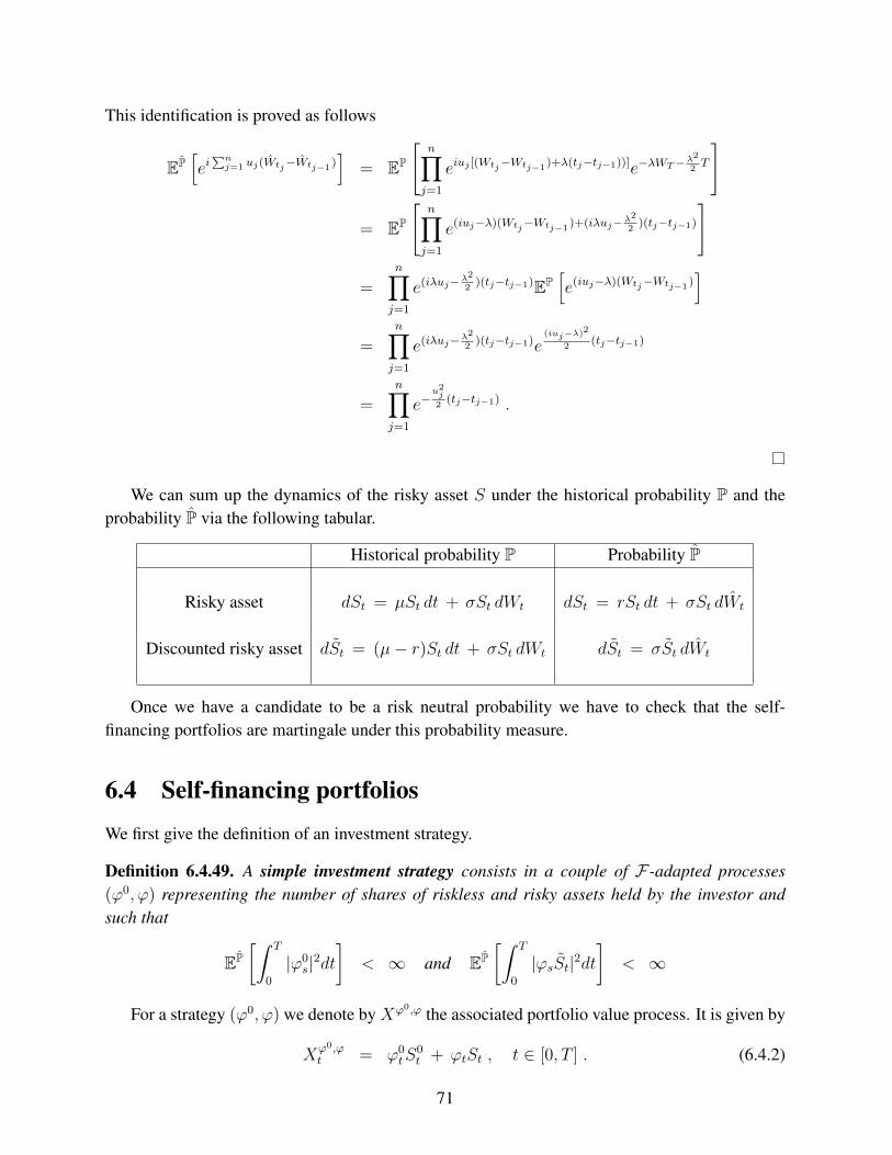
This identification is proved as follows

EP[ei∑nj=1 uj(Wtj−Wtj−1 )

]= EP

[n∏j=1

eiuj [(Wtj−Wtj−1 )+λ(tj−tj−1))]e−λWT−λ2

2T

]

= EP

[n∏j=1

e(iuj−λ)(Wtj−Wtj−1 )+(iλuj−λ2

2)(tj−tj−1)

]

=n∏j=1

e(iλuj−λ2

2)(tj−tj−1)EP

[e(iuj−λ)(Wtj−Wtj−1 )

]=

n∏j=1

e(iλuj−λ2

2)(tj−tj−1)e

(iuj−λ)2

2(tj−tj−1)

=n∏j=1

e−u2j2

(tj−tj−1) .

We can sum up the dynamics of the risky asset S under the historical probability P and theprobability P via the following tabular.

Historical probability P Probability P

Risky asset dSt = µSt dt + σSt dWt dSt = rSt dt + σSt dWt

Discounted risky asset dSt = (µ− r)St dt + σSt dWt dSt = σSt dWt

Once we have a candidate to be a risk neutral probability we have to check that the self-financing portfolios are martingale under this probability measure.

6.4 Self-financing portfolios

We first give the definition of an investment strategy.

Definition 6.4.49. A simple investment strategy consists in a couple of F-adapted processes(ϕ0, ϕ) representing the number of shares of riskless and risky assets held by the investor andsuch that

EP[∫ T

0

|ϕ0s|2dt

]< ∞ and EP

[∫ T

0

|ϕsSt|2dt]

< ∞

For a strategy (ϕ0, ϕ) we denote by Xϕ0,ϕ the associated portfolio value process. It is given by

Xϕ0,ϕt = ϕ0

tS0t + ϕtSt , t ∈ [0, T ] . (6.4.2)

71

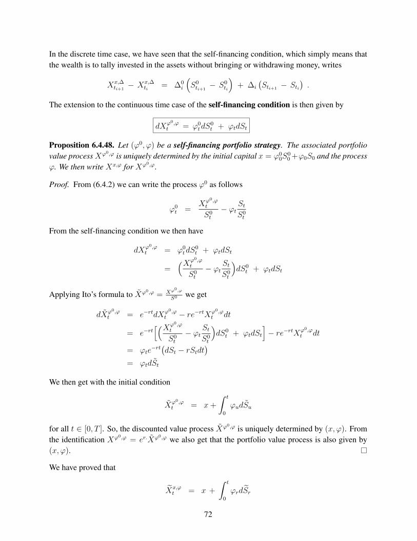
In the discrete time case, we have seen that the self-financing condition, which simply means thatthe wealth is to tally invested in the assets without bringing or withdrawing money, writes

Xx,∆ti+1− Xx,∆

ti = ∆0i

(S0ti+1− S0

ti

)+ ∆i

(Sti+1

− Sti).

The extension to the continuous time case of the self-financing condition is then given by

dXϕ0,ϕt = ϕ0

tdS0t + ϕtdSt

Proposition 6.4.48. Let (ϕ0, ϕ) be a self-financing portfolio strategy. The associated portfoliovalue processXϕ0,ϕ is uniquely determined by the initial capital x = ϕ0

0S00 +ϕ0S0 and the process

ϕ. We then write Xx,ϕ for Xϕ0,ϕ.

Proof. From (6.4.2) we can write the process ϕ0 as follows

ϕ0t =

Xϕ0,ϕt

S0t

− ϕtStS0t

From the self-financing condition we then have

dXϕ0,ϕt = ϕ0

tdS0t + ϕtdSt

=(Xϕ0,ϕ

t

S0t

− ϕtStS0t

)dS0

t + ϕtdSt

Applying Ito’s formula to Xϕ0,ϕ = Xϕ0,ϕ

S0 we get

dXϕ0,ϕt = e−rtdXϕ0,ϕ

t − re−rtXϕ0,ϕt dt

= e−rt[(Xϕ0,ϕ

t

S0t

− ϕtStS0t

)dS0

t + ϕtdSt

]− re−rtXϕ0,ϕ

t dt

= ϕte−rt(dSt − rStdt)

= ϕtdSt

We then get with the initial condition

Xϕ0,ϕt = x+

∫ t

0

ϕudSu

for all t ∈ [0, T ]. So, the discounted value process Xϕ0,ϕ is uniquely determined by (x, ϕ). Fromthe identification Xϕ0,ϕ = er.Xϕ0,ϕ we also get that the portfolio value process is also given by(x, ϕ).

We have proved that

Xx,ϕt = x +

∫ t

0

ϕrdSr

72

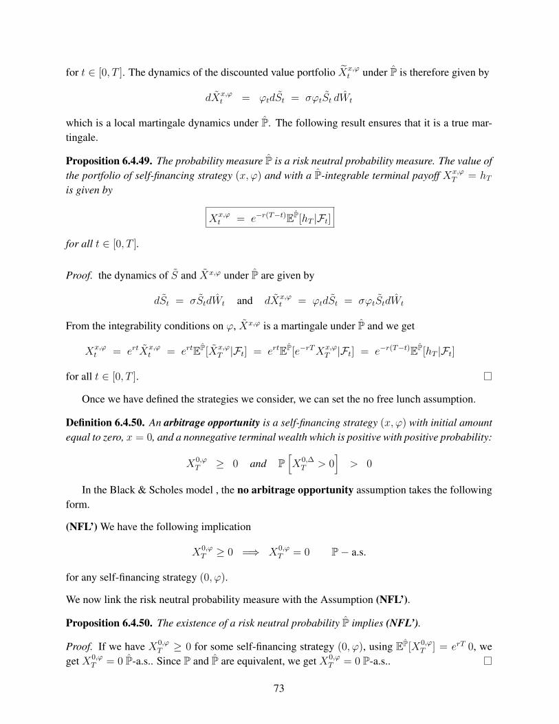
for t ∈ [0, T ]. The dynamics of the discounted value portfolio Xx,ϕt under P is therefore given by

dXx,ϕt = ϕtdSt = σϕtSt dWt

which is a local martingale dynamics under P. The following result ensures that it is a true mar-tingale.

Proposition 6.4.49. The probability measure P is a risk neutral probability measure. The value ofthe portfolio of self-financing strategy (x, ϕ) and with a P-integrable terminal payoff Xx,ϕ

T = hTis given by

Xx,ϕt = e−r(T−t)EP[hT |Ft]

for all t ∈ [0, T ].

Proof. the dynamics of S and Xx,ϕ under P are given by

dSt = σStdWt and dXx,ϕt = ϕtdSt = σϕtStdWt

From the integrability conditions on ϕ, Xx,ϕ is a martingale under P and we get

Xx,ϕt = ertXx,ϕ

t = ertEP[Xx,ϕT |Ft] = ertEP[e−rTXx,ϕ

T |Ft] = e−r(T−t)EP[hT |Ft]

for all t ∈ [0, T ].

Once we have defined the strategies we consider, we can set the no free lunch assumption.

Definition 6.4.50. An arbitrage opportunity is a self-financing strategy (x, ϕ) with initial amountequal to zero, x = 0, and a nonnegative terminal wealth which is positive with positive probability:

X0,ϕT ≥ 0 and P

[X0,∆T > 0

]> 0

In the Black & Scholes model , the no arbitrage opportunity assumption takes the followingform.

(NFL’) We have the following implication

X0,ϕT ≥ 0 =⇒ X0,ϕ

T = 0 P− a.s.

for any self-financing strategy (0, ϕ).

We now link the risk neutral probability measure with the Assumption (NFL’).

Proposition 6.4.50. The existence of a risk neutral probability P implies (NFL’).

Proof. If we have X0,ϕT ≥ 0 for some self-financing strategy (0, ϕ), using EP[X0,ϕ

T ] = erT 0, weget X0,ϕ

T = 0 P-a.s.. Since P and P are equivalent, we get X0,ϕT = 0 P-a.s..

73

We can now give the definition of the price of a contingent claim.

Theorem 6.4.18. Let C be a contingent claim. All the self financing strategies (x, ϕ) that replicateC have the same initial capital x = P0(C) given by

P0(C) =1

S0T

EP[C] .

P0(C) is called the price of the contingent claim C.

Proof. Let (x, ϕ) and (x′, ϕ′) be two self-financing strategies replicating C. Then we have

Xx,ϕT = Xx′,ϕ′

T = C .

Since Xx,ϕ and Xx′,ϕ′ are martingales under P we get

x =1

S0T

EP[Xx,ϕT ] =

1

S0T

EP[C] ,

x′ =1

S0T

EP[Xx′,ϕ′

T ] =1

S0T

EP[C] .

Therefore, we get x = x′ = P0(C).

6.5 Duplication of a financial derivative

We first provide a Markov property for the process S.

Lemma 6.5.2. Let h : R → R be a measurable function such that the random variable h(ST ) isP-integrable. Then there exists a measurable function v : [0, T ]× R+ → R such that

v(t, St) = e−r(T−t)EP[h(ST )|Ft]

for all t ∈ [0, T ].

Proof. Recall that in the Black & Scholes model the value of the underlying asset S is given by

St = S0 e

(r−σ

2

2

)t−σWt

for any t ∈ [0, T ]. We then deduce that

ST = St e

(r−σ

2

2

)(T−t)−σ(WT−Wt) .

The conditional expectation can then be written

e−r(T−t)EP[h(ST )|Ft] = e−r(T−t)EP[h

(St e

(r−σ

2

2

)(T−t)−σ(WT−Wt)

)|Ft]

74

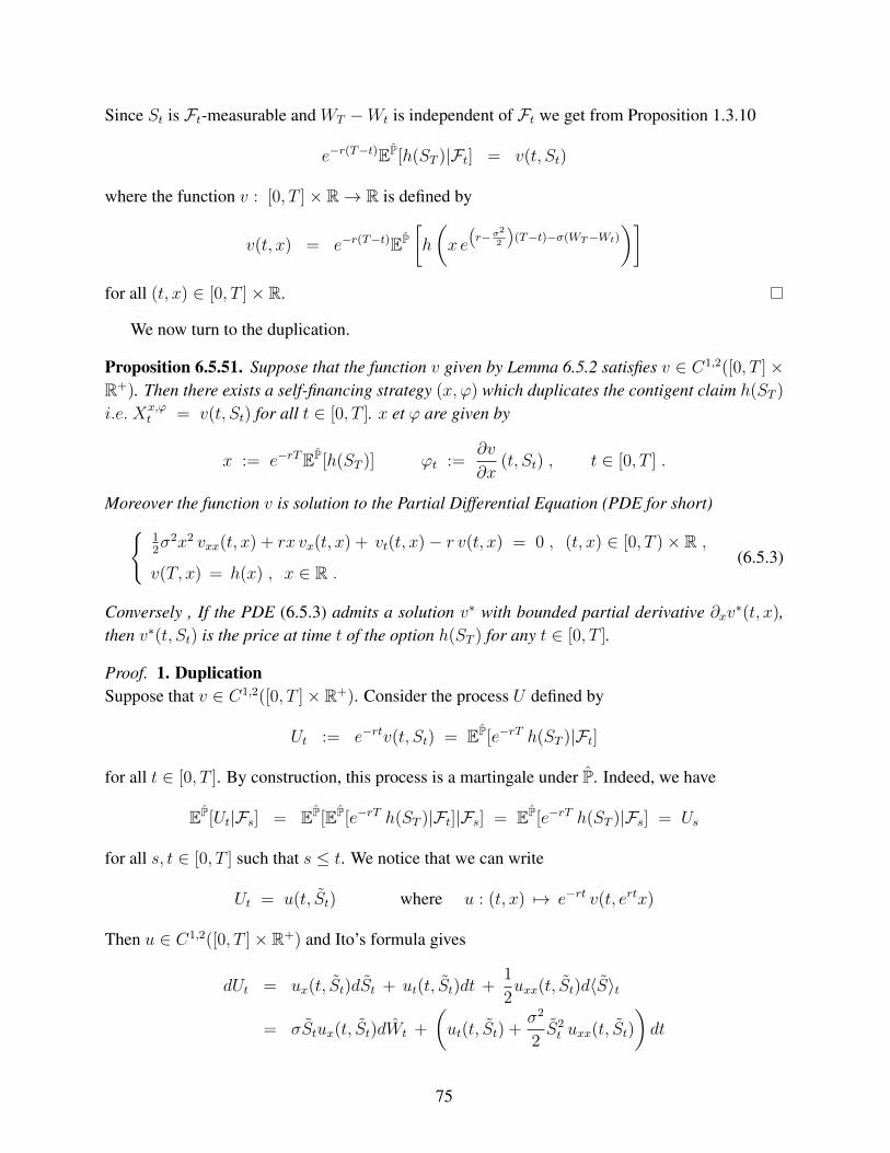
Since St is Ft-measurable and WT −Wt is independent of Ft we get from Proposition 1.3.10

e−r(T−t)EP[h(ST )|Ft] = v(t, St)

where the function v : [0, T ]× R→ R is defined by

v(t, x) = e−r(T−t)EP[h

(x e

(r−σ

2

2

)(T−t)−σ(WT−Wt)

)]for all (t, x) ∈ [0, T ]× R.

We now turn to the duplication.

Proposition 6.5.51. Suppose that the function v given by Lemma 6.5.2 satisfies v ∈ C1,2([0, T ]×R+). Then there exists a self-financing strategy (x, ϕ) which duplicates the contigent claim h(ST )

i.e. Xx,ϕt = v(t, St) for all t ∈ [0, T ]. x et ϕ are given by

x := e−rTEP[h(ST )] ϕt :=∂v

∂x(t, St) , t ∈ [0, T ] .

Moreover the function v is solution to the Partial Differential Equation (PDE for short)12σ2x2 vxx(t, x) + rx vx(t, x) + vt(t, x)− r v(t, x) = 0 , (t, x) ∈ [0, T )× R ,

v(T, x) = h(x) , x ∈ R .(6.5.3)

Conversely , If the PDE (6.5.3) admits a solution v∗ with bounded partial derivative ∂xv∗(t, x),then v∗(t, St) is the price at time t of the option h(ST ) for any t ∈ [0, T ].

Proof. 1. DuplicationSuppose that v ∈ C1,2([0, T ]× R+). Consider the process U defined by

Ut := e−rtv(t, St) = EP[e−rT h(ST )|Ft]

for all t ∈ [0, T ]. By construction, this process is a martingale under P. Indeed, we have

EP[Ut|Fs] = EP[EP[e−rT h(ST )|Ft]|Fs] = EP[e−rT h(ST )|Fs] = Us

for all s, t ∈ [0, T ] such that s ≤ t. We notice that we can write

Ut = u(t, St) where u : (t, x) 7→ e−rt v(t, ertx)

Then u ∈ C1,2([0, T ]× R+) and Ito’s formula gives

dUt = ux(t, St)dSt + ut(t, St)dt +1

2uxx(t, St)d〈S〉t

= σStux(t, St)dWt +

(ut(t, St) +

σ2

2S2t uxx(t, St)

)dt

75

The process U is an Ito process and also a martingale. Thus its finite variation part, i.e. its “dt”part, is equal to zero and we get

Ut = U0 +

∫ t

0

ux(r, Sr)dSr .

for all t ∈ [0, T ]. Consider the self-financing strategy (x, ϕ) given by

x := U0 = e−rTEP[h(ST )] and ϕt := ux(t, St) = e−rtvx(t, St) , t ∈ [0, T ] .

By construction, U is a true martingale so (x, ϕ) is a portfolio strategy (it satisfies the integrabilityconditions) and from the self-financing condition, the dicounted value of the associated portfoliois given by

Xx,ϕt = x +

∫ t

0

ϕr dSr = U0 +

∫ t

0

ux(r, Sr)dSr = Ut

for all t ∈ [0, T ]. The portfolio Xx,ϕ, is therefore a duplication portfolio since it satisfies

Xx,ϕT = erTUT = v(T, ST ) = e−r(T−T )EP[h(ST )|FT ] = h(ST ) .

2. Valuation PDEThe process U is a martingale under P. Thus its “dt” part is equal to zero:

ut(t, St) +1

2σ2S2

t uxx(t, St) = 0

for all t ∈ [0, T ]. This allows to get

ut(t, x) +1

2σ2S2

t uxx(t, x) = 0

for all (t, x) ∈ [0, T )× Rd. [The idea replace St by any deterministic point x is to say that W is aBrownian motion under P and it therefore can move to any point of R. Since σ > 0 is is the samefor S.] From the definition of u, we have

ut(t, x) = −r e−rt v(t, ertx) + e−rt vt(t, ertx) + rx vx(t, e

rtx)

uxx(t, x) = (ert)2 vxx(t, ertx)

for all (t, x) ∈ [0, T )× Rd. We therefore get the following PDE for v

1

2σ2S2

t vxx(t, St) + rSt vx(t, St) + vt(t, St)− r v(t, St) = 0

for all (t, x) ∈ [0, T )× R with the terminal

3. ReverseLet v∗ be a smooth solution to PDE (6.5.3). Let us introduce the process U∗t := e−rtv∗(t, St),t ∈ [0, T ], and u∗ the associated function. From Ito’s fomula the dynamics of U∗ is the given by

dU∗t = σStu∗x(t, St)dWt +

(u∗t (t, St) +

1

2σ2S2

t u∗xx(t, St)

)dt

76

Since v∗ is solution to PDE (6.5.3) the “dt” part is equal to zero and we get

U∗t = U0 +

∫ t

0

u∗x(r, Sr)dSr

for all t ∈ [0, T ]. Since the derivative v∗x is bounded, we get the same for u∗x and therefore U∗ is amartingale under P. we then deduce that

v∗(t, St) = ert U∗t = ert EP[U∗T |Ft] = e−r(T−t) EP[h(ST )|Ft]

for all t ∈ [0, T ]. So v∗(t, St) is the price at time t of the contingent claim h(ST ).

Remark 6.5.29. The assumption v ∈ C1,2([0, T ]×R+) is not very restrictive. In a first approach,on can belive that we need the payoff h to be smooth. However, thanks to the expectation operatoron the definition of the price, the function v can be seen as a convolution product between thefunction h and the density of the standard Gaussian law which makes v smooth.

6.6 Black & Scholes formula

At a time t ∈ [0, T ], the price of the contingent claim h(ST ) is given by v(t, St) with

v(t, St) = e−r(T−t)EP[h(ST )|Ft]

and the function v is solution to the Balck & Scholes PDE (6.5.3).For somepay-off functions h it is possible to get a closed fomula for the price at any time

t ∈ [0, T ] of the contigent claim h(ST ). It the case of the Call and Put options.

Proposition 6.6.52. In the Black & Scholes model, the price of a call option with maturity T andstrike K is given by

Ct = StN (d1) − K e−r(T−t)N (d2) , t ∈ [0, T ] ,

where N is the cumulative distribution function of the standard Gaussian Law N (0, 1), d1 et d2

are given by

d1 :=ln(St

K) + (r + σ2

2)(T − t)

σ√T − t

and d2 := d1 − σ√T − t .

The Call Put parity formula is the following

Ct − Pt = St − Ke−r(T−t) , t ∈ [0, T ] .

The price of the Put option with maturity T and strike K is given by

Pt = K e−r(T−t)N (−d2) − StN (−d1) , t ∈ [0, T ] .

77

Proof. Price of the Call option. The price of the Call option at a time t ∈ [0, T ] is given by

Ct = e−r(T−t)EP[(ST −K)+|Ft] = e−r(T−t)EP[(St e

(r−σ2

2)(T−t) +σ(WT−Wt) −K

)+

|Ft].

As we have already seen Ct = v(t, St) with v given by

v(t, x) = e−r(T−t)EP[(x e(r−σ

2

2)(T−t) +σ(WT−Wt) −K

)+].

Consider the exercise region E defined by

E =x e(r−σ

2

2(T−t) +σ(WT−Wt) > K

=

Wt − WT√T − t

<ln( x

K) + (r − σ2

2)(T − t)

σ√T − t

We can then write Ct with E as follows

Ct = xEP[eσ(WT−Wt)− σ2

2)(T−t)1E

]− K e−r(T−t) P(E)

We now Introduce the probability measure P∗ equivalent to P and defined by

dP∗

dP

∣∣∣∣FT

= ZT := eσWT − σ2

2T .

We then notice that E is independent of Ft. This gives

EP[1EZTZt

]= EP∗

[1E

1

Zt

]= EP∗ [1E ] EP∗

[1

Zt

]= P∗(E)

Therefore, we can rewrite v(t, x) as follows

v(t, x) = xP∗(E) − K e−r(T−t) P(E) .

From Girsanov theorem, the process W ∗ defined by W ∗t := Wt − σt, t ∈ [0, T ] is a Brownian

motion under P∗. We then rewrite E with W ∗ as follows

E =

Wt − WT√T − t

<ln( x

K) + (r − σ2

2)(T − t)

σ√T − t

=

W ∗t −W ∗

T√T − t

<ln( x

K) + (r + σ2

2)(T − t)

σ√T − t

.

Since Wt−WT√T−t and W ∗t −W ∗T√

T−t follow a standard Gaussian law N (0, 1) respectively under P and P∗,the call price can be written

Ct = v(t, St) = StN (d1) − K e−r(T−t)N (d2) .

Price of the Put option. We obtain the price of the Put Option by using the Call-Put parity relationthe the identity N (x) +N (−x) = 1 for all x ∈ R.

Remark 6.6.30. The price of the call option at time t is of the form C(T − t, σ, St, r,K). Itsatisfies the homogeneity property

C(T − t, σ, λ St, r, λK) = λC(T − t, σ, St, r,K) .

78

6.7 Greeks

The sensitivities of the price of an option with respect to its different parameters are called theGreeks:

– the Delta ∆ is the sensitivity of the option price w.r.t. the present value of the underlying,

– the Theta θ is the sensitivity of the option price w.r.t. the present time t,

– the Vega ϑ (unfortunately, it is not a Greek letter) is the sensitivity of the option price w.r.t.the volatility;

– the Rho ρ is the sensitivity of the option price w.r.t. the interest rate r,

– the Gamma Γ is the sensitivity of the delta w.r.t. the present value of the underlying.

The PDE (6.5.3) can then be written

1

2σ2 x2 Γ + r x∆ − r P + θ = 0 .

For a Call Option, the sensitivities at t = 0 are given by

∆ = N (d1) > 0 Γ =1

xσ√TN ′(d1) > 0 ρ = TKe−rTN (d2) > 0

θ = − xσ

2√TN ′(d1) − K r e−rTN (d2) < 0 ϑ = x

√TN ′(d1) > 0

For a Put option, the sensitivities at t = 0 are given by

∆ = −N (−d1) > 0 Γ =1

xσ√TN ′(d1) > 0 ρ = TKe−rT (N (d2)− 1) < 0

θ =xσ

2√TN ′(d1) + K r e−rT (N (d2)− 1) ϑ = x

√TN ′(d1) > 0

The Delta can be interpreted as the number of shares of risky asset in the duplication portfolio.The Gamma measures the rate of change in the delta with respect to the changes of the underlyingasset. It is used to decide the intervention frequency for the hedging portfolio.

The Vega is used to know the dependence of the price w.r.t. the volatility. It is important, sinceit can measure the model error e.g. in calibration methods.

The Theta measures the decrease of the option price w.r.t. time.The dependence of the prices of a Call and a Put Option in their different parameters are the

following

∆ Θ ϑ ρ Γ

Call + − + + +

Put − ? + − +

79

6.8 Exercices

6.8.1 Option valuation in the Black & Scholes model

We consider a financial market composed by a riskless asset S0 defined by its initial value S00 and

its dynamic

dS0t = rS0

t dt , t ∈ [0, T ] ,

and a risky asset S defined by its initial value S0 and its dynamic

dSt = µStdt+ σStdWt , t ∈ [0, T ] .

where W is a standard Brownian motion.

1. Give the expression of S0t for all t ∈ [0, T ].

2. Prove the existence and uniqueness of the process S and give the expression of St for allt ∈ [0, T ].

3. We denote by St the discounted value at time t of the risky asset. Give the SDE satisfied by Son [0, T ].

4. We define the process W par

Wt = Wt +µ− rσ

t , t ≥ 0 .

Write the dynamics of the process S with the process W .

5. Prove that there exists a probability measure P equivalent to P under which W is a standardBrownian motion.

6. Prove that S is a martingale under P.

7. Deduce that for any self-financing strategy (x, ϕ) satisfying the admissibility condition

EP[ ∫ T

0

|ϕsS1t |2dt

]<∞ , (6.8.4)

the discounted portfolio Xx,ϕ is a martingale.

8. We aim at pricing the option with terminal pay-off GT given by

GT =∣∣ST −K∣∣

We admit that such a contingent claim is duplicable by a self financing strategy satisfying condition(6.8.4). Write the price G0 at time t = 0 of this contingent claim as an expectation.

9. Calculate G0 as a function of r, σ, K and T .

80

6.8.2 Put option with mean strike

Let S be the process defined by S0 = 1 and

dSt = St(rdt+ σdWt

), t ∈ [0, T ]

with r and σ two constants such that σ > 0. We aim at calculating

C := EP[(ZT − ST )+]

where

ZT = exp( 1

T

∫ T

0

ln(St)dt)

Let Q be the probability measure defined by its density

dQdP

∣∣∣∣FT

= eσWT−σ2

2T .

1. Give the expression of the process S.

2. Prove that

EQ[(ZTST− 1)+]

= e−rTEP[(ZT − ST )+]

3. By applying Ito’s formula to the process (tWt)t∈[0,T ], write∫ T

0Wtds − TWT as a stochastic

integral w.r.t. W .

4. Deduce from the previous question that ZTST

can be written under the form eαT−∫ T0 β(t)dWt , where

α and β have to be determined.

5. Let W be the process defined by

Wt := Wt − σt , t ∈ [0, T ] .

Write ZTST

under the form eαT−∫ T0 β(t)dWt , where α and β have to be determined.

6. Prove that 1T

∫ T0β(t)dWt and W 1

T2

∫ T0 β(t)2dt have the same law.

7. Find a constant K such that the computation of C reduces to the computation of the quantity

E[(S 1T2

∫ T0 β2(t)dt −K

)+]

where S is a geometric Brownian motion that has to be detailed.

81

6.8.3 Asian Option

Let S be the process defined by

St = S0 +

∫ t

0

rSudu+

∫ t

0

σSudWu , t ∈ [0, T ] ,

where r and σ are two constants.

1. Prove the existence and uniqueness of the process S and give its expression.

2. Let K be a constant. Prove that the process M defined by

Mt = E[( 1

T

∫ T

0

Srdr −K)+∣∣∣Ft] , t ∈ [0, T ] ,

is a martingale.

3. Define the process Q by

Qt =1

St

(K − 1

T

∫ t

0

Sudu), t ∈ [0, T ] .

Prove that we have

Mt = StE[( 1

T

∫ T

t

SuStdu−Qt

)+∣∣∣Ft]for all t ∈ [0, T ].

4. Let u : [0, T ]× R→ R be the function defined by

u(t, x) = E[( 1

T

∫ T

t

SuStdu− x

)+]

Prove that

u(t, x) = E[( 1

T

∫ T

t

SuStdu− x

)+∣∣∣Ft]for all (t, x) ∈ [0, T ]× R and that

Mt = Stu(t, Qt)

for all t ∈ [0, T ].

4. We suppose that the function u is smooth. Apply Ito’s formula to M and deduce the PDEsatisfied by the function u.

82