One People - One Goal - One Faith

MINISTRY OF ECONOMY AND FINANCE

DEPARTMENT OF FORECASTING AND

ECONOMIC STUDIES

Study N°25

Agricultural Policy, Productivity and Long Run Economic Growth in Senegal

DPEE/DEPE @ August 2013

1

Alsim FALL Baidy Baro MBAYE Hamat SY1

August 2013

ABSTRACT

Senegalese agricultural sector appears to be unproductive in light of low performances over the last decades. This study attempts to assess and analyze the effects of Senegalese current agricultural policy on growth,

particularly through an increase in productivity. A special attention is paid to newly-implemented agricultural programs in the Public Investment

Triennial Plan (PITP), which estimated cost is FCFA 126 billion. To measure these effects, we set up an agricultural-based Computable General Equilibrium Model. Our main result shows that the agricultural sector

activity could rise up to 10.7% per year in average, during 2014-2023. However, this outcome could be halved by ineffective investment spending or

poor investment monitoring.

JEL Classification: Q11, Q18, H3, C68

Keywords: Agricultural policy, productivity, economic growth, CGE Model

1 We thank the researchers Alioune Dieng, DIA Djiby and Cheikh Sadibou FALL (Senegalese Institute of Agricultural Research) and the National Accountant Fode DIEME (National Agency of Statistics and Demography) for their distinguished contribution to the realization of this document.

Agricultural Policy, Productivity et Long Run Economic Growth in Senegal

2

I. INTRODUCTION

Since its independence, Senegal has successively identified several strategies for agricultural

development in order to give the sector its importance due to economic growth, redistribution

of income and food security. Thus, starting from a highly interventionist agricultural policy

during the first two decades of independent Senegal, the Government has subsequently

gradually withdrawn in favor of structural adjustment policies (SAP) signed with

Brettonwoods institutions. This withdrawal took place through the New Agricultural Policy

(NAP), whose implementation began in 1984.

The liberalization of agricultural sector has become more effective in the late 1990s, but it

was from the 2000s that new guidelines have been established with the adoption in 2004 of

the Framework “Loi Agro-Silvo-Pastoral” (LOASP) and its annexes programs. In addition,

the state launched in 2006, the plan for the Return to Agriculture (REVA), hoping to stem

migration of young Senegalese to Europe. Then, in 2008, Great Agricultural Offensive for

Food and Abundance (GOANA) was implemented in response to the global food crisis of

2007-2008. Furthermore, Senegal has developed its National Agricultural Investment

Program (NAIP), from a common vision established at the continental (through CAADP) and

sub-regional (through ECOWAP).

Thus, the agricultural policy of Senegal is designed through several strategic documents that

may cause a difficult implementation. In spite of all efforts for its development, Senegalese

agriculture remains unproductive in terms of performances for decades. During the last fifteen

years, its contribution to economic growth is almost null (0.1%), and its share in GDP

increased from 10% in 1997 to less than 8% in 2011. Labor productivity in agricultural sector

remains very low compared to secondary and tertiary sectors. It also shows a highly volatile

growth rates.

However, hope for the emergence of a thriving agricultural sector is still allowed if one refers

to the renewed political will of the Senegalese public authorities have placed agriculture at

the heart of economic and social development process. Therefore, the issue of the relevance of

the new direction of agricultural policy deserves special consideration, both on government

than that of academic research. This study is in this perspective and seeks to assess and

analyze the effects of the current agricultural policy of Senegal on growth, particularly

through increased productivity. The paradox that agriculture concentrates 28% of the active

population and provides only 7.8% of production, is sufficiently illustrative of productivity

3

issues submitted this sector. This study attempts to identify and levers and constraints of the

agricultural policy of Senegal that govern the evolution of agricultural growth. Therefore, it

will be possible to discuss the conditions under which agricultural policy could be consistent

with the National Strategy for Economic and Social Development (SNDES) which expects a

sustained growth in the medium and long term, 7-8%.

Moreover, in front of the plurality of agricultural policy documents, the study focuses on

agricultural projects and programs outlined in the Triennial Public Investment Program

(PTIP). Indeed, the PTIP is the convergence framework and implementation of all public

projects and programs. It is implemented over a period of 3 years, according to a rolling

program. However, it is important to note that only the additional spending on agriculture are

are analyzed because other agricultural expenses are assumed to evolve according to the trend

of the economy. Thus, new agricultural programs have been added to PTIP (2012-2014),

while other programs, existing, recorded an increase in their allocation. Overall, the

programmed budget in PTIP (2013-2015) increased 126.034 billion FCFA compared to the

previous TIPI (2012-2014).

A dynamic CGE model is used to evaluate the sectorial and macroeconomic effects of

additional expenditures envisaged in agricultural policy. Note that the CGE is designed to

take into account a comprehensive agricultural sector at its most representative sectors. Using

a CGE model is important in more ways than one, as it allows both to quantify the economic

impact in the short and medium term of the increase in public spending (demand effects) and

to assess the structuring effects of long-term (supply effects), which primarily affect the

production function of agricultural units.

The rest of the paper is as follows. Section 2 traces the history of agricultural development

strategies put in place since the early years of independence. Section 3 analyzes in detail the

costs of additional investments to be implemented in 2013-2015. The stylized facts are

presented in Section 4. Section 5 reviews the theoretical and empirical literature on the effects

of agricultural policy on growth and productivity. Section 6 discusses the essential points of

the CGE and explains how agricultural policy is supported by the model. The results and their

interpretation are presented in Section 7. Finally, Section 8 is reserved for the conclusion.

4

II. REVIEW OF AGRICULTURAL DEVELOPMENT STRATEGIES IN

SENEGAL

During the first two decades following Senegal's independence, the Government conducted an

interventionist agricultural policy in order to intensify and diversify agricultural production.

Thus, management structures, as the “Office de Commercialisation Agricole du Sénégal”

(OCAS) were created to support farmers and disseminate farming methods and techniques.

The OCAS had the privilege of purchasing monopoly on groundnut production from

agricultural cooperatives and a limited number of approved private traders. Then, the Office

sold the harvest to processing plants operating in Senegal or companies which organized the

export of groundnut for its treatment in France.

An ambitious program of agricultural modernization had been set up, funded by the BSD

(Senegalese Bank of Senegal), later BNDS (National Bank of Development of Senegal). It

was supervised by the CRAD (Regional Centers for Development Assistance) and accessible

to farmers through cooperatives which guaranteed borrowings, based on Groundnut sales

produced by their members. Between 1966 and 1967 the CRAD and OCAS were dissolved

and their functions were transferred to the « National Office of Cooperation and Assistance

Development » (ONCAD), a newly created structure.

Faced with persistent imbalances that affected the senegalese economy in the late 70s and the

vulnerability of public finances, the Government was obliged to adopt adjustment’measures in

the agricultural sector. Consequently, the Stabilization Program was implemented in 1979 and

the Economic and Financial Recovery Program between 1980 and 1984. Thus ONCAD was

dissolved in 1980 and its businesses acquired by the National Company of Commercialization

of oleaginous of Senegal (SONACOS). The disengagement of the Government has been

strengthened by the official end of the agricultural program and fertilizer credit. Instead, the

Government tried to establish a restraint on Groundnut sales (the refund) for the repayment of

fertilizer loans in 1984. During the same year, the Government has adopted the "New

Agricultural Policy" (NPA) which further reduces its interventionist action in the agricultural

sector. The NPA has sought to create conditions for the revival of production, in a framework

that promotes effective participation and empowerment of the rural areas.

However, following the devaluation of the CFA and in order to correct the dysfunctions

5

observed in the implementation of the NPA, the Government has implemented the "Structural

Adjustment Policy of Agriculture" (PASA), which setting execution is ensured via the Letter

for Agricultural Development Policy (LPDA) in April 1995. The withdrawal of the

Government, initiated in 1979, is widely deepened by the LPDA.

The willingness of the government to develop the agricultural sector can also be seen through

the development and approval of the various sectorial policy documents, including the

Development Policy Letter for the agricultural sector Institutional (LPI 1998), the Letter of

Decentralized Rural Development Policy (LPDRD, 1999) and the Development Policy Letter

from the Groundnut Die (2003).

The liberalization of the agricultural sector becomes more effective in 1997, but the results are

inconclusive. In addition, the integration of the Senegalese agricultural sector liberalized in

the world market and the greater autonomy of farmers, show a lack of training for agricultural

professionals. In 1999, the National Strategy for Agricultural and Rural Training (SNFAR)

was set up with the objectives to be achieved by 2015.

From the 2000s, the agricultural sector poor performance have succeeded, forcing the political

authorities to implement a new, more comprehensive agricultural issues, in order to put

agriculture at the heart of the strategy for high and sustainable growth. In particular,

agricultural organizations, including the National Council for Dialogue and Cooperation of

Rural (NCRC), requested a new farm bill. Thus, the Orientation Law Agro-Silvo-Pastoral

(LOASP) of 2004 was enacted to give an overall strategic direction to Senegalese agriculture

over a period of 20 years, based on the strengthening of family farms. This law is the basis for

development of medium term operational programs, such as the National Agriculture

Development Programme (NADP), the National Programme for Livestock Development

(PNDE) and the Forestry Action Plan of Senegal (PAFS). LOASP has therefore replaced all

sectorial agricultural policies in Senegal. It is supposed to be made operational by the

agricultural component of the PRSP later became the SED, then SNDES.

6

GraphII.1 : Multiplicity of agricultural policy documents

???

?

???

?

Note : NEPAD (Nouveau Partenariat pour le Développement de l'Afrique), PDDAA (Programme Détaillé de

Développement de l’Agriculture en Afrique), ECOWAP (Politique agricole de la CEDEAO), PNIA (Programme national

d’Investissement agricole), LOASP (Loi d’Orientation Agro-Sylvo-Pastorale), PNDA (Programme National de

Développement Agricole), PNDE (Plan national de développement de l’Elevage), PADPA (Plan d’action pour le

développement de la Pêche et de l’Aquaculture), PAFS (Plan d’Action Forestier du Sénégal), DSRP (Document de

Stratégie de Réduction de la Pauvreté), DPES (Document de Politique Economique et Sociale), SNDES (Stratégie

Nationale de Développement Economique et Social), PTIP (Programme triennal d’Investissement public).

The current state reveals an agricultural policy designed through several strategic documents

that can cause a difficult implementation. Indeed, apart from the programs launched under the

LOASP, the Government launched, in 2006, the Plan for Return to Agriculture (REVA) to

deal with illegal immigration flows to Europe , Senegalese youth who, for lack of better,

embarked in canoes to travel often marred by high seas drama. This program had, at once, two

major objectives: revitalize agriculture and enable young emigrants to return to Senegal,

investing in agriculture. Finally in 2008, the state launched the Great Agricultural Offensive

for Food and Abundance (GOANA) in response to the global food crisis of 2007-2008. Its

PNDA

PND

E

NEPAD

LOASP

PADP

A PDDAA

PAFS

Volet Agriculture

(DSRP, DPES, SNDES) ECOWAP

PNIA Programmes

Agricoles

(PTIP)

7

aim was to meet the challenge of food sovereignty, to avoid any risk of famine or starvation,

and produce for export.

In a spirit of coordination of national policies, sub-regional and regional, the african countries

adopted the New Partnership for Africa's Development (NEPAD), which agricultural

component is supported by the Comprehensive Development Programme Agriculture in

Africa (CAADP). This is implemented in West Africa through the Agricultural Program of

ECOWAS (ECOWAP) and nationally by the National Agricultural Investment Program

(NAIP). Note finally that the objectives of the LOASP are supposed to put in harmony with

those of the ECOWAP / CAADP.

III. FUNCTIONAL DISTRIBUTION OF ADDITIONAL EXPENSES

Senegal's agricultural policy is defined in several strategies formulated at regional, sub-

regional and national levels. In front of the plurality of agricultural policy documents, it

should focus on agricultural projects and programs written in the Triennial Public Investment

Program (PTIP). Indeed, this document is the convergence and implementation framework of

all public projects and programs. It is implemented over a period of three years following a

rolling program. However, it should be noted that only the additional spending on agriculture

must be subject to analysis because other agricultural expenses are assumed to evolve

according to the trend of the economy.

Overall, the programmed budget in PTIP (2013-2015) increased 126.034 billion CFA francs,

compared to the previous PTIP (2012-2014). Thus, new agricultural programs are added to

PTIP (2012-2014), while other programs already existing recorded an increase of their

allocation. These programs are listed in the following table

8

Table III.1 : Increased investment spending on agriculture (in millions Francs CFA)

PROJETS/PROGRAMMES Symbole 2013 2014 2015 TOTAL Financement

Nouveaux Projets/Programmes

Amélioration de la productivité agricole/WAPP-Phase II prog1 2 500 4 500 8 500 15 500 BM/BCI-ETAT

Projet de développement inclusif et durable de l’agrobusiness prog2 300 1 500 2 000 3 800 BM

Fonds d’entretien et de maintenance des infrastructures hydro-agricoles prog3 1 285 1 500 1 715 4 500 BCI-ETAT

Appui à la sécurité alimentaire dans la région de Matam prog4 800 3 650 6 150 10 600 EU-FED/AFD/BCI-ETAT

Appui à la sécurité alimentaire à Louga, Kaffrine et Matam prog5 500 2 000 3 000 5 500 BAD-FAD

Appui au programme national d’investissement agricole prog6 700 4 000 6 000 10 700 ITALIE

Appui à la production durable du riz pluvial à Kaolack, Kaffrine et Fatick prog7 500 1 050 1 100 2 650 JAPON/BCI-ETAT

Fonds de Garantie des Investissements Prioritaires (FONGIP) prog8 5 000 5 000 5 000 15 000 BCI-ETAT

Projet de construction et réhabilitation de pistes communautaires prog9 500 2 000 3 000 5 500 BAD-FAD

Projet d’appui à la sécurité alimentaire (insertion des jeunes) prog10 300 475 475 1 250 FONDS KOWEITIEN

Projets/Programmes ayant bénéficie de crédits supplémentaires

Programme d’équipement du monde rural prog11 3 667 3 667 3 667 11 000 BCI-ETAT

Programme de reconstitution du capital semencier prog12 3 667 3 667 3 755 11 088 BCI-ETAT

Programme national d’insertion et développement agricole prog13 2 200 2 567 938 5 705 BM/ESPAGNE/BCI-

ETAT Programme national d’autosuffisance en riz (réfection des aménagements hydro agricoles)

prog14 2 933 4 906 4 400 12 240 BM/BCI-ETAT

Dotation au fonds de sécurisation du crédit rural (garantie, bonification, calamités). prog15 2 567 4 033 4 400 11 000 BCI-ETAT

dont garantie 1 467 2 200 2 200 5 867

dont bonification 367 733 1 100 2 200

dont calamités 733 1 100 1 100 2 933

TOTAL GENERAL 27 419 44 515 54 100 126 034

Source : PTIP

9

Moreover, these investments are mainly used to increase the stock of capital and

infrastructure, improve the productivity of factors and facilitate access to credit. At this level,

assumptions were made to distribute, at best, the planned expenditure according to their

attributes and objectives. Thus, the budget "equipment program of the rural area" should be

allocated to the increase in equipment of agricultural chains, in proportion to the size of their

capital stock. In addition, the Paddy Rice also benefit from an increase in equipment through

the "supporting the sustainable production of upland rice in Kaolack, Fatick and Kaffrine"

program. However, this program can increase both cultivable areas as infrastructure dedicated

to the rice. Thus, its budget is divided in proportion to the size of each of these factors used in

the production of paddy rice.

Table III.2 : Spending on the increase of capital stock (million CFA)

CHAINS INCREASE IN CAPITAL STOCK

Equipments Land Infrastructures

FOOD AGRICULTURE

Maize 302 0 76

Rice paddy 1 760 2 058 390

Millet 1 744 0 437

Other Food. Agr. 4 313 0 1 081

INDUSTRIAL AGRICULTURE

Groundnut 2 394 0 595

Coton 81 0 20

Tomatoe 291 0 72

Sugar cane 114 0 28

Others Ind. Agr. 516 0 128

TOTAL 11 515 2 058 2 828

Source : PTIP, authors’ calculations

The increase in agricultural infrastructure stock is mainly supported by half of the budget of

the "construction and community roads rehabilitation projects." The other part should be used

for the rehabilitation of agricultural infrastructure that improves productivity. Overall, the

additional expense allocated to the increase in inventory would be about 16.4 billion FCFA

(13% of the supplementary budget).

10

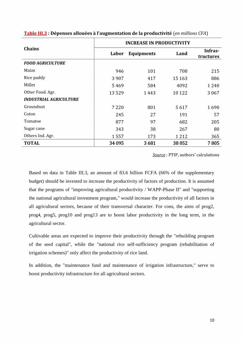
Table III.3 : Dépenses allouées à l’augmentation de la productivité (en millions CFA)

Chains INCREASE IN PRODUCTIVITY

Labor Equipments Land Infras-

tructures

FOOD AGRICULTURE

Maize 946 101 708 215

Rice paddy 3 907 417 15 163 886

Millet 5 469 584 4092 1 240

Other Food. Agr. 13 529 1 443 10 122 3 067

INDUSTRIAL AGRICULTURE

Groundnut 7 220 801 5 617 1 690

Coton 245 27 191 57

Tomatoe 877 97 682 205

Sugar cane 343 38 267 80

Others Ind. Agr. 1 557 173 1 212 365

TOTAL 34 095 3 681 38 052 7 805

Source : PTIP, authors’ calculations

Based on data in Table III.3, an amount of 83.6 billion FCFA (66% of the supplementary

budget) should be invested to increase the productivity of factors of production. It is assumed

that the programs of "improving agricultural productivity / WAPP-Phase II" and "supporting

the national agricultural investment program," would increase the productivity of all factors in

all agricultural sectors, because of their transversal character. For cons, the aims of prog2,

prog4, prog5, prog10 and prog13 are to boost labor productivity in the long term, in the

agricultural sector.

Cultivable areas are expected to improve their productivity through the "rebuilding program

of the seed capital", while the "national rice self-sufficiency program (rehabilitation of

irrigation schemes)" only affect the productivity of rice land.

In addition, the "maintenance fund and maintenance of irrigation infrastructure," serve to

boost productivity infrastructure for all agricultural sectors.

11

Table III.4 : Dépenses allouées à l’accès au crédit (en millions CFA)

CHAINS ACCESS TO CREDIT

FOOD AGRICULTURE

Maize 713

Rice paddy 2945

Millet 4122

Other Food. Agr. 10195

INDUSTRIAL AGRICULTURE

Groundnut 5658

Coton 192

Tomatoe 687

Sugar cane 269

Others Ind. Agr. 1220

TOTAL 26 000

Source : PTIP, authors’ calculations

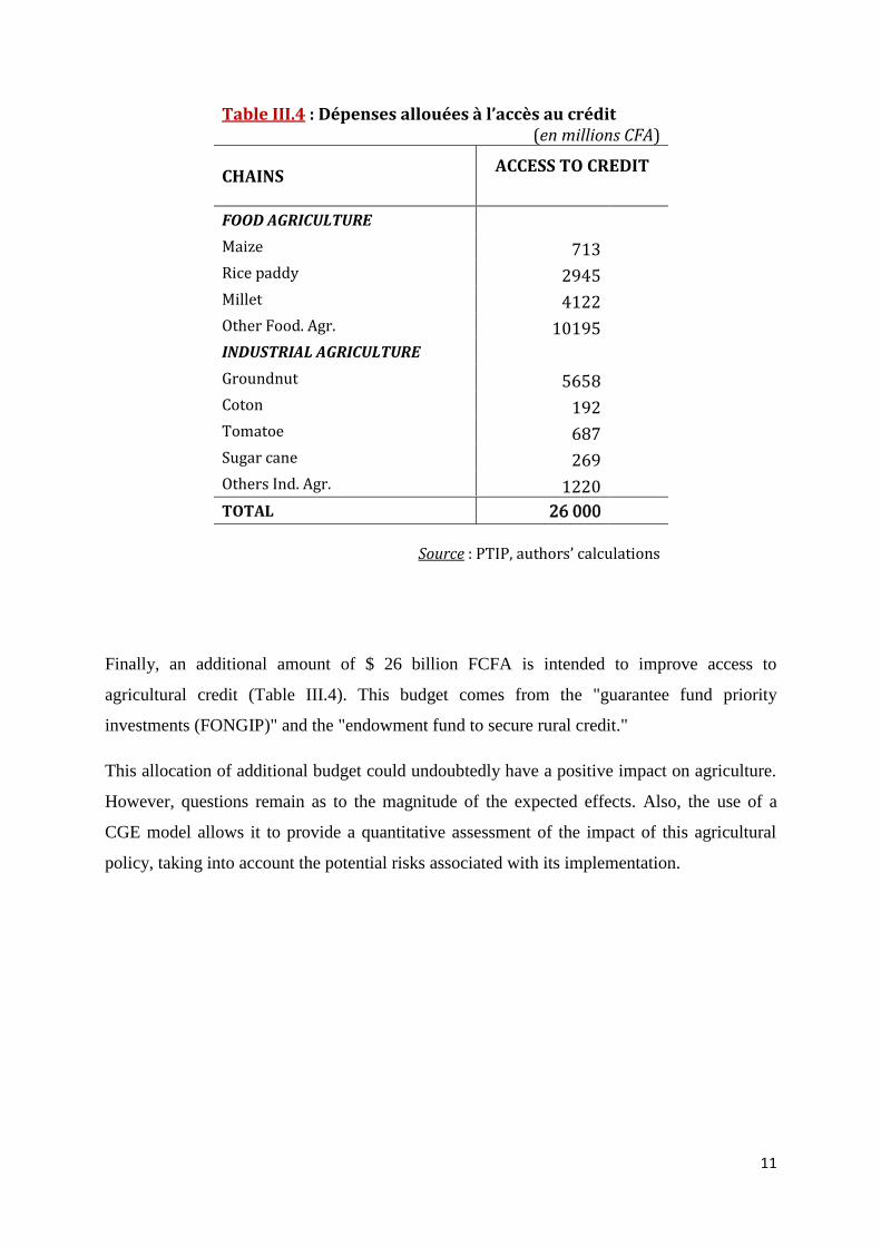
Finally, an additional amount of $ 26 billion FCFA is intended to improve access to

agricultural credit (Table III.4). This budget comes from the "guarantee fund priority

investments (FONGIP)" and the "endowment fund to secure rural credit."

This allocation of additional budget could undoubtedly have a positive impact on agriculture.

However, questions remain as to the magnitude of the expected effects. Also, the use of a

CGE model allows it to provide a quantitative assessment of the impact of this agricultural

policy, taking into account the potential risks associated with its implementation.

12

IV. STYLIZED FACTS ON SENEGALESE AGRICULTURE

IV.1. Background

IV.1.1. Analysis of agricultural growth

Senegalese agriculture is mainly composed of cash crops (groundnuts, cotton, sugar cane),

food crops (rice, maize, millet, sorghum, cowpea, cassava) and horticulture (fruits and

vegetables). The annuity business is largely dominated by the cultivation of groundnuts. Food

agriculture products, mainly consisting of cereals, fall, in large part, to the final consumption

of households.

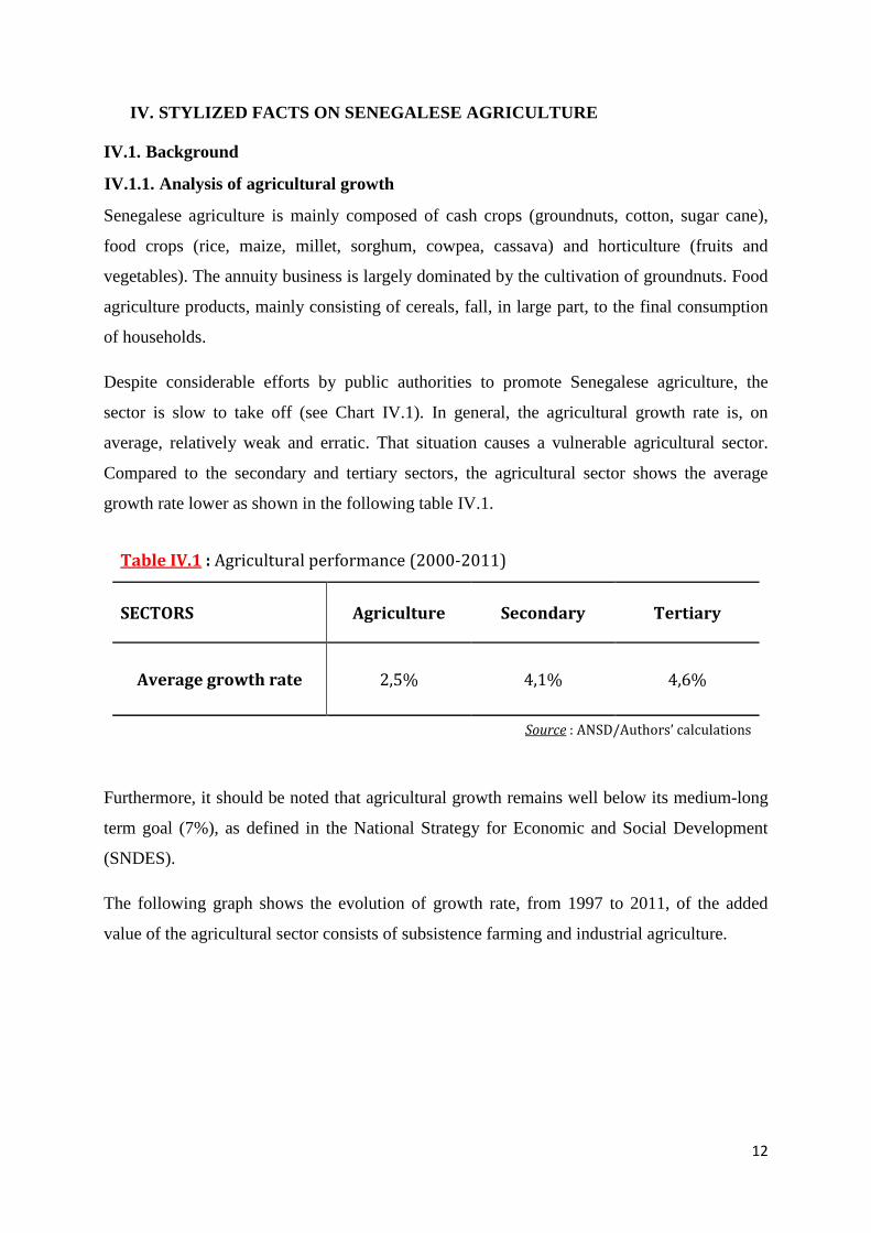
Despite considerable efforts by public authorities to promote Senegalese agriculture, the

sector is slow to take off (see Chart IV.1). In general, the agricultural growth rate is, on

average, relatively weak and erratic. That situation causes a vulnerable agricultural sector.

Compared to the secondary and tertiary sectors, the agricultural sector shows the average

growth rate lower as shown in the following table IV.1.

Table IV.1 : Agricultural performance (2000-2011)

SECTORS Agriculture Secondary Tertiary

Average growth rate 2,5% 4,1% 4,6%

Source : ANSD/Authors’ calculations

Furthermore, it should be noted that agricultural growth remains well below its medium-long

term goal (7%), as defined in the National Strategy for Economic and Social Development

(SNDES).

The following graph shows the evolution of growth rate, from 1997 to 2011, of the added

value of the agricultural sector consists of subsistence farming and industrial agriculture.

13

GRAPHIV.1 : Evolution of the agricultural sector growth rate (1997-2011)

Source : ANSD

After a decline in 1997, the agricultural value added registered a positive growth that was

maintained until 2000, before declining in 2001 and further deteriorate to a record level of -

34.5% in 2002. Indeed, 2002 coincided with the decline in agricultural production due, in

large part, to the off-season rains and flooding along the Gambia River.

As usual, after a drastic decline, agricultural value added has returned to growth in 2003, also

supported by good rainfall and implementation of programs, especially for corn.

In 2004, year of the LOASP’s adoption, there has been a slight increase in agricultural value

added (4.1%), driven by industrial agriculture (25.8%), despite a decline in food crops (-5%).

Exogenous factors, including the locust threat and rainfall deficit, have, in fact, characterized

the 2004/2005 crop year, causing the decline of food crops. Thus grain production declined by

25.3%, while groundnut production rose by 36.7%.

Agricultural value added grew by 16% in 2005. This performance can be explained by a good

distribution of rainfall in time and space, the renewal of agricultural equipment, subsidized

price to the availability of good quality inputs and a good plant health monitoring.

-80%

-60%

-40%

-20%

0%

20%

40%

60%

80%1

,99

7

1,9

98

1,9

99

2,0

00

2,0

01

2,0

02

2,0

03

2,0

04

2,0

05

2,0

06

2,0

07

2,0

08

2,0

09

2,0

10

2,0

11

Agriculture vivriere Agriculture industrielle ou d'exportation Agriculture

14

However, agricultural growth was negative for 2006 and 2007. The underperformance is

mainly due to lower plantings and yields, the late implementation of fertilizers and seeds, to

unfavorable climatic conditions and difficulties related to previous commercialization

campaigns.

In 2008, strong growth was recorded, due to what may be called the "green revolution." This

revolution has been materialized by the creation of the Great Agricultural Offensive for Food

and Abundance (GOANA). However, the various stimulus plans of Senegalese agriculture did

not allow a continuation of agricultural performance. Indeed, from 2009, the sector has

gradually deteriorated peaking at a negative growth rate of 27.8% in 2011. This decrease is

equivalent to a loss of 113 billion of value added in 2011 compared to 2010.

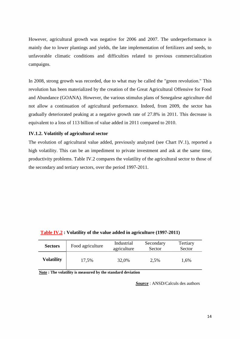
IV.1.2. Volatitily of agricultural sector

The evolution of agricultural value added, previously analyzed (see Chart IV.1), reported a

high volatility. This can be an impediment to private investment and ask at the same time,

productivity problems. Table IV.2 compares the volatility of the agricultural sector to those of

the secondary and tertiary sectors, over the period 1997-2011.

Table IV.2 : Volatility of the value added in agriculture (1997-2011)

Sectors Food agriculture Industrial

agriculture

Secondary

Sector

Tertiary

Sector

Volatility 17,5% 32,0% 2,5% 1,6%

Note : The volatility is measured by the standard deviation

Source : ANSD/Calculs des authors

15

Industrial agriculture is more volatile (32%) than subsistence farming (17.5%). Indeed,

Groundnut, which is the main speculative industrial agriculture, is heavily dependent on

rainfall. However, Senegal has suffered severe climatic irregularities during the fifteen year

period.

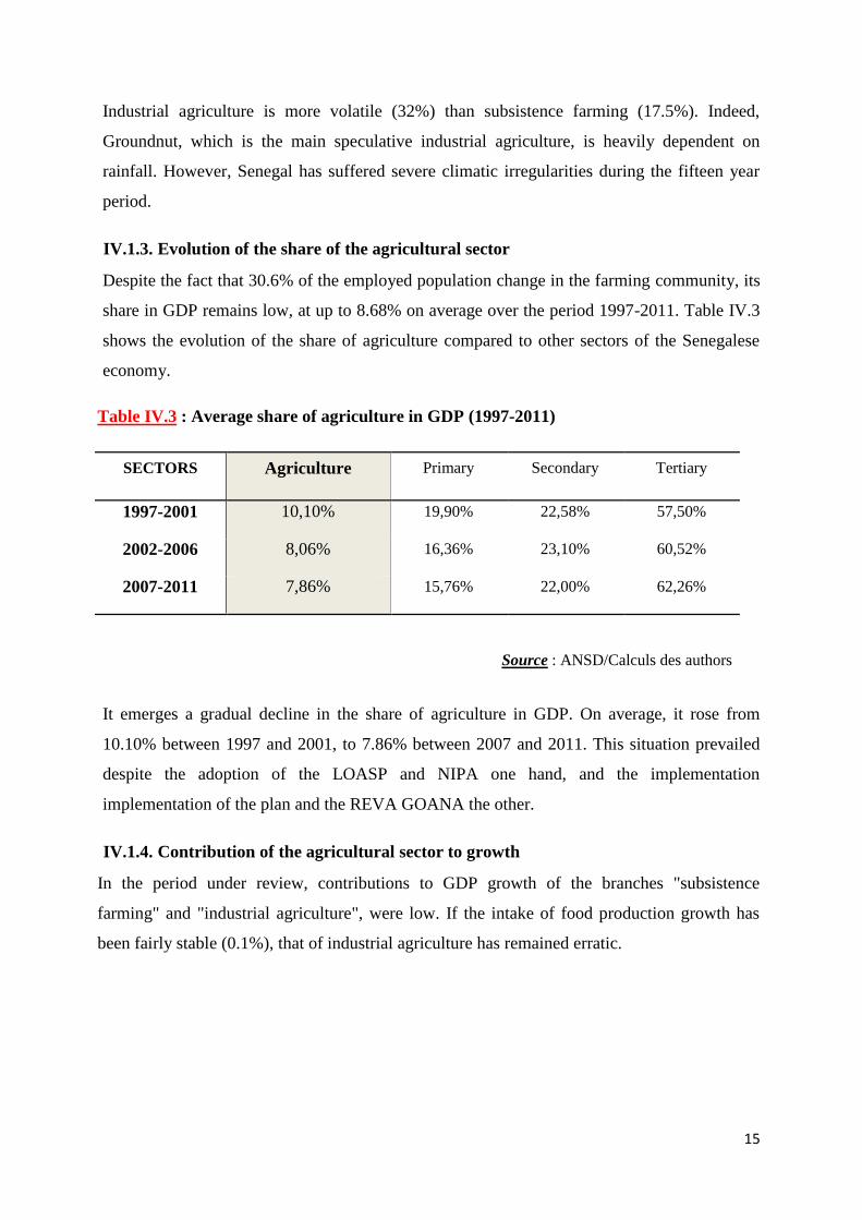
IV.1.3. Evolution of the share of the agricultural sector

Despite the fact that 30.6% of the employed population change in the farming community, its

share in GDP remains low, at up to 8.68% on average over the period 1997-2011. Table IV.3

shows the evolution of the share of agriculture compared to other sectors of the Senegalese

economy.

Table IV.3 : Average share of agriculture in GDP (1997-2011)

SECTORS Agriculture Primary Secondary Tertiary

1997-2001 10,10% 19,90% 22,58% 57,50%

2002-2006 8,06% 16,36% 23,10% 60,52%

2007-2011 7,86% 15,76% 22,00% 62,26%

Source : ANSD/Calculs des authors

It emerges a gradual decline in the share of agriculture in GDP. On average, it rose from

10.10% between 1997 and 2001, to 7.86% between 2007 and 2011. This situation prevailed

despite the adoption of the LOASP and NIPA one hand, and the implementation

implementation of the plan and the REVA GOANA the other.

IV.1.4. Contribution of the agricultural sector to growth

In the period under review, contributions to GDP growth of the branches "subsistence

farming" and "industrial agriculture", were low. If the intake of food production growth has

been fairly stable (0.1%), that of industrial agriculture has remained erratic.

16

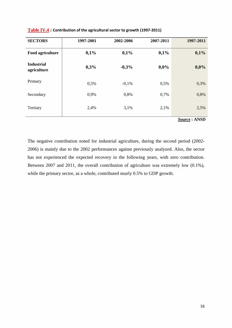
Table IV.4 : Contribution of the agricultural sector to growth (1997-2011)

SECTORS 1997-2001 2002-2006 2007-2011 1997-2011

Food agriculture 0,1% 0,1% 0,1% 0,1%

Industrial

agriculture 0,3% -0,3% 0,0% 0,0%

Primary 0,5% -0,1% 0,5% 0,3%

Secondary 0,9% 0,8% 0,7% 0,8%

Tertiary 2,4% 3,1% 2,1% 2,5%

Source : ANSD

The negative contribution noted for industrial agriculture, during the second period (2002-

2006) is mainly due to the 2002 performances against previously analyzed. Also, the sector

has not experienced the expected recovery in the following years, with zero contribution.

Between 2007 and 2011, the overall contribution of agriculture was extremely low (0.1%),

while the primary sector, as a whole, contributed nearly 0.5% to GDP growth.

17

IV.1.5. Agricultural labor's contribution

The role of agricultural workforce also deserves emphasis, which simultaneously raises

questions about productivity. Indeed, the agricultural population is very important and

represent 28% of the working population in 2011. The graph below shows the evolution of

labor parallel to that of the added value.

GRAPHIV.2 : Value added and labor in the agricultural sector (1997-2011)

Source : ANSD

The growth of the agricultural labor force in the fifteen years (1.9%) has been slow, compared

to that of the working population (3%). Indeed, labor migration has become a reality in

Senegal, causing the exodus of the rural farm population to urban areas.

These movements are due, among other things, to resources scarcity and rural drought. This

translates, mechanically, by a slightly positive growth in agricultural labor productivity.

Indeed, all things being equal, growth in agricultural value added (3.2%), combined with

weak growth in agricultural labor, suggesting a trend increase in agricultural labor

productivity.

0

50

100

150

200

250

300

350

400

450

0

200

400

600

800

1,000

1,200

1,400

1,9

97

1,9

98

1,9

99

2,0

00

2,0

01

2,0

02

2,0

03

2,0

04

2,0

05

2,0

06

2,0

07

2,0

08

2,0

09

2,0

10

2,0

11

POPULATION ACTIVE AGRICOLE VALEUR AJOUTEE

Po

pu

lati

on

(e

n m

illi

ers

d'a

ctif

s)

Va

leu

r a

jou

tée

(e

n m

iili

ard

s d

e F

CF

A)

18

IV.2. Analysis of key sectors

IV.2.1. Maize

Corn became, in 2003, the second grain speculation after millet, thanks to the special

program, launched by the senegalese Government, which permitted to achieve a growth rate

of 399% (Multiple Appearance by ...) compared to 2002. However, performance waned from

2006 when production fell by 54.6%. Despite a substantial recovery observed in 2008

(151.1%), with the establishment of the GOANA, production has recovered to decrease from

2010.

Difficulties in the sector are mainly related to low price incentives, soil fertility, climatic

hazards and dilapidated farm equipment. These constraints pose damaging productivity

problems in the sector. They lead to the failure of the industry to meet local demand, leading

to a rise in imports.

GRAPHIV.3 : Maiz imports (en tons)

Source : ANSD

The volume of maize imports has consistently believed. However, periods of decline were

recorded in 2004, due to the corn program, and in 2009 and 2010, after the launch of

GOANA.

IV.2.2. Rice

Rice is the staple food consumption in Senegal. However, a huge gap exists between domestic

demand and local production.

The government, keen to develop the rice sector, created in 1965, the National Development

Corporation and exploitation of River delta lands Senegal and Falémé (SAED). This company

had the facilities to work and management of irrigation and also worked for inputs and

agricultural advice. Thereafter, the rice sector was liberalized in 1996. This liberalization has

-

20,000

40,000

60,000

80,000

100,000

120,000

20

00

20

01

20

02

20

03

20

04

20

05

20

06

20

07

20

08

20

09

20

10

20

11

19

also affected rice imports because the domestic rice production only allowed to cover between

20 and 30% of domestic demand. However, in 2008, the national rice self-sufficiency (RAN)

was launched in order to reduce dependency on the outside.

The constraints of rice in Senegal are related to important bird invasions, especially in the

Senegal River Valley, the dilapidated processing plants that alter the quality of the rice

husking, difficulties in marketing of local rice, the low level of use mineral fertilizers and

quality seeds, inputs access problems on time, credit access difficulties and land issues.

To these various constraints in the sector, add the high and growing amount of rice imports, as

indicated in the chart below.

GRAPHIV.6 : Broken rice imports (tons)

Source : ANSD

Rice imports ranged, on average, to 729,021 tons over the period, against 288,497 tons for

local production. However, they dropped from 2008, due to the performance recorded in rice

caused by the REVA plan and the GOANA. Unfortunately, like corn, rice imports have

returned to growth in 2011.

-

200,000

400,000

600,000

800,000

1,000,000

1,200,000

19

97

19

98

19

99

20

00

20

01

20

02

20

03

20

04

20

05

20

06

20

07

20

08

20

09

20

10

20

11

20

IV.2.3. Groundnuts

Groundnut is the major source of income for the rural world. This sector is also one of the

first four Senegal's export products, with fishery products, phosphates, and tourism. The

Groundnut production activity in Senegal has a significant ripple effect on other sectors (the

collection, industrial processing and marketing of products).

However, the groundnut sector faces the constraints of climate disruption, degradation of

soils, deficiencies in inputs supply, especially seeds, of lack of renewal and maintenance of

equipment park, the lack of support / advice to producers and access to credit. To these are

added the difficulties of groundnut marketing.

In 2013, Chinese traders arrived on the Senegalese market Groundnuts, proposing a producer

price which approximates 250FCFA kilo, different from the official price of 190FCFA. The

arrival of China on the groundnut market brought a financial windfall for producers who think

they can make a decent living from selling their produce at this price. However, this situation

is detrimental to local mills (SUNEOR, NOVASEN) likely to suffer from a lack of supplies in

.

IV.2.4. Cotton

Cotton cultivation began in Senegal after gaining independence, thanks to the French Textile

Development Company (CFDT), and highly dependent agriculture diversification sake of

Groundnut.

Sodefitex (textile fibers Development Corporation), which was created in 1974, adopted a

strategy for intensifying cotton cultivation. She contributed to the development of the sector,

in distributing free inputs to cotton producers and putting in place in the early 80s, a

functional literacy policy for the training of village technical relays.

However, cotton production has fallen particularly from 2008. The difficulties of the cotton

crop are often related to irregular rainfall, the weakness of production, price volatility of the

fiber, the traffic of subsidized inputs by the State, pest pressure and over-indebtedness of

cotton farmers (about 1, 8 billion FCFA in 2011) following the crisis of 2000-2010.

21

IV.2.5. Garden products: tomato and onion

IV.2.5.1. Tomatoes

Tomato is the second horticultural speculation after onion. It is a diversified culture for the

Senegal River Valley specialized in irrigated rice. The elements that benefit tomato growers

in this area are the existence of processing plant and irrigation schemes.

However, the constraints of collective dependence vis-à-vis the credit, the obsolescence of

agricultural machinery, evacuation of production to factories, competition from growing

imposed by importing triple tomato paste and the high cost of some agricultural inputs,

including fertilizer, affect the sector.

IV.2.5.2. Oinions

The onion had its emergence through agricultural production diversification policy of Senegal

in the early 70. Like other horticultural products, it also was an alternative to the nutritional

balance of the population was threatened by drought. The proceeds from the sale of onion was

also additional income for farmers and a reduction component of the balance of trade deficit.

The problems in the sector mainly concern the degradation of groundwater, the little

reassuring land situation, lack of resources, difficulties in access to credit, lack of storage

facilities and marketing competition from imported onion.

IV.3. Agricultural productivity

Agricultural productivity seems to be the best barometer of agricultural development as

measuring the effectiveness of agricultural practices. However, it remains low in Senegal, due

to constraints related to land degradation, climate irregularities, locust invasions, the low

quality seeds, outdated farming equipment and lack of training of farmers.

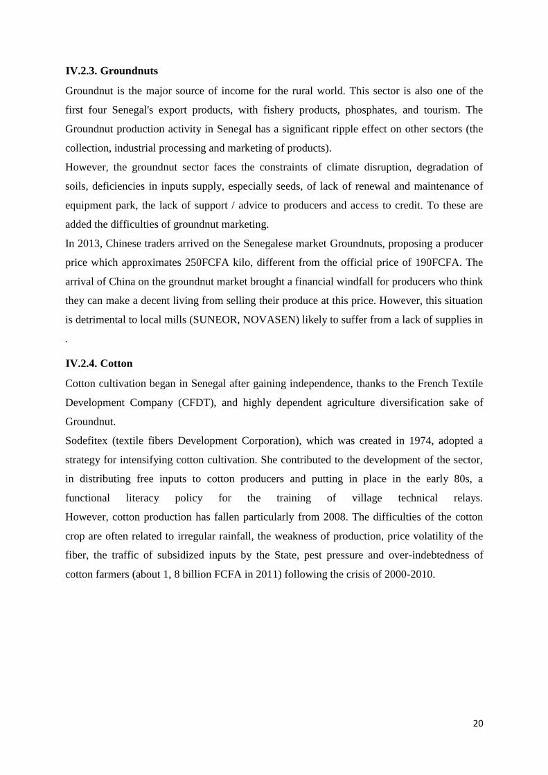
The major factor in agricultural production is largely made up by the earth. The graphs below

put in relation the growth rate of productivity with that of acreage for food crops and

industrial agriculture.

22

GRAPHIV.7 : Relationship between cultivated area and productivity (1997-2011)

food agriculture

industrial agriculture

Source : ANSD

The negative slopes indicate that the productivity moves in the opposite direction relative to

the surface. Thus, the land extension policy does not necessarily lead to higher productivity.

This observation can probably help explain why GOANA was not a great success, although it

has attracted an extension of more than 40% of the cultivated area. However, it is important to

qualify this, because of the limitations of the single-factor productivity.

In terms of labor productivity, it provides information on the ability of farmers to optimize

production. The graph below compares labor productivity of the agricultural sector to other

sectors.

-100%

-50%

0%

50%

100%

150%

-40% -20% 0% 20% 40% 60% 80%

Ta

ux

de

cro

issa

nce

de

la

pro

du

ctiv

ité

Growth area

-25%

-20%

-15%

-10%

-5%

0%

5%

10%

15%

20%

25%

30%

-40% -20% 0% 20% 40% 60%

Growth area

Ta

ux

de

cro

issa

nce

de

la

pro

du

ctiv

ité

23

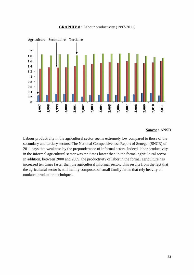
GRAPHIV.8 : Labour productivity (1997-2011)

Source : ANSD

Labour productivity in the agricultural sector seems extremely low compared to those of the

secondary and tertiary sectors. The National Competitiveness Report of Senegal (SNCR) of

2011 says that weakness by the preponderance of informal actors. Indeed, labor productivity

in the informal agricultural sector was ten times lower than in the formal agricultural sector.

In addition, between 2000 and 2009, the productivity of labor in the formal agriculture has

increased ten times faster than the agricultural informal sector. This results from the fact that

the agricultural sector is still mainly composed of small family farms that rely heavily on

outdated production techniques.

0

0.2

0.4

0.6

0.8

1

1.2

1.4

1.6

1.8

2

1,9

97

1,9

98

1,9

99

2,0

00

2,0

01

2,0

02

2,0

03

2,0

04

2,0

05

2,0

06

2,0

07

2,0

08

2,0

09

2,0

10

2,0

11

Secondaire Agriculture Tertiaire

24

V. THEORETICAL AND EMPIRICAL LITERATURE REVIEW

Agricultural productivity refers to the efficiency with which farmers combine inputs to

produce outputs. This is an important factor in profitability and competitiveness of the

agricultural sector. Solow (1957) growth in production is largely due to an increase in

productivity. Furthermore, Hayami and Ruttan (1985) showed that agricultural production can

increase in two ways. First, the output growth may be due to an increase in the use of land,

capital, labor and intermediate consumption. Second, the growth of agricultural production

can be brought about by advances in production techniques. The following paragraphs explain

the main determinants and the different methods of measuring agricultural productivity.

Empirical work on the impact of productivity improvements in agricultural production, are

also discussed.

V.1. Determinants of agricultural productivity

The literature on the determinants of agricultural productivity, provides information on the

levers that public authorities must take action to increase agricultural performance. Overall,

agricultural productivity can be improved for inputs that enter directly into the production

process, but also through an environment conducive to the development of the sector.

In a study of soil quality, agricultural productivity and food security, Wiebe (2003) showed

that land degradation does not threaten food security globally, but there are serious problems

in areas where the soils are fragile, insecure property rights and farmers' access to information

and markets, limited. In most cases, soil quality varies agro-ecological zones and geographical

conditions. So Gisselquist (1999) highlighted the geography and agricultural productivity in

India. His analysis shows that differences in grain yield between the northern states of central

and southern India, are strongly linked to the regional geographic variation. It has some effect

on productivity, all other things being equal. The authors show also that precipitation and

temperature in tropical and dry states influence yields higher food grains.

In addition, the analysis of the effects of migration on agricultural productivity is attracting

more and more attention of researchers. As such, Rozelle et al. (1999) attempted to establish

links between remittances, migration and the Chinese agricultural productivity. Labor

migration is, indeed, an important phenomenon that affects economic development and

modernization. The study showed, through a simple econometric regression that migration has

a negative impact on agricultural productivity, the influx of rural population to urban areas

greatly reducing agricultural labor. Nevertheless, the negative effects of this phenomenon on

25

productivity are mitigated by remittances of migrants who contribute significantly to mitigate

food insecurity.

The development of agriculture needs a good framework that allows farmers to produce in

optimal conditions, feeding decently and market in the best part of their production. Antle

(1983), concerned about the agricultural practice environment, showed the importance of the

development of infrastructure in increasing agricultural productivity. As expected, the impact

of infrastructure on agricultural productivity was positive. The development of agriculture in a

country is largely dependent on the existence of good infrastructure, especially in transport

and communication. Also, it is important to modernize and develop agricultural practices. In

this sense, Alston (2010) conducted a comprehensive review of the literature on the role of

innovation and R & D in the growth of agricultural productivity. It concludes that the

investment rate of return on R & D is generally high. For its part, Kussa (2012), was

interested in the effects of the health of farmers on agricultural productivity in Ethiopia.

Patients farmers, on average, a score of 33.5% in terms of technical efficiency, against 48.9%

in healthy households. The author shows, and that the establishment of an adequate health

system helps to increase the productivity of farmers.

V.2. Measures of agricultural productivity

The measurement of agricultural productivity is the subject of much controversy. The

accuracy and precision in the definition of agricultural productivity and in the designation of

its determinants, in theory, are most obvious when it comes to empirical cases. Indeed, the

constraints related to the availability of statistical invite themselves very often in this exercise.

An index of production on a particular input is often used to measure the partial productivity

of a factor. This type of indicator used to measure the time course of the unit production of a

given input. For example, the yield per hectare is used to measure the productivity of the land,

while output per worker quantifies the productivity of labor. However, partial productivities

measures factors have shortcomings when it comes to capture technology. Indeed, they do not

reflect changes in input use.

In contrast, total factor productivity (TFP) is a ratio that relates the aggregation of all the

outputs with the aggregation of all inputs. It measures in a simple way, the efficiency with

which inputs are transformed into outputs. However, different methods of aggregation of

inputs and / or outputs can lead to different estimates, each consistent with the production

function under - lying specified. TFP indices used in the literature are generally Laspeyres,

Paasche, Fisher, Törnqvist-Theil and Elteto-Köves-Szulc (EKS).

26

TFP offers many advantages, in that it is clearly defined, easily measurable and offers

possibilities for comparison over time and across different studies. It also constitutes a

privileged tool for the analysis of the effectiveness of policies designed to increase the

economic well-being, even if the effects of government policies on agricultural productivity

can be offset and that other factors influence productivity. Thus the MFP generic term is often

preferred to that of TFP that some input and / or output are necessarily excluded from the

analysis, according to the availability of statistics.

Without loss of generality, the TFP growth has three components (Coelli et al., 2005):

technological change, changes in technical efficiency and changes in scale efficiency. In this

sense, Darku, Malla and Tran (2012) measured the changes in total factor productivity of

Canadian agriculture, using the approach of the stochastic frontier. The results of the

decomposition of TFP in technological development, scale effect and changes in technical

efficiency, showed that productivity changes are primarily driven by technological change.

27

V.3. Application of CGE model in agriculture

According Savard (1995), originally mainly two reasons justified the use of CGE models in

agriculture. The first is related to the pressure in favor of liberalization of agricultural policies

in the context of the GATT multilateral negotiations, with the consolidation of trading blocs

such as the EU and NAFTA. The second is, in turn, related to the reappraisal of the

interventionist role of the States, imposed by budget constraints. So many CGE were built to

analyze the impact of the proposed agricultural liberalization in the Uruguay Round. Other

models have, for cons, analyzed agricultural policy changes on the overall economy and the

well-being.

Burniaux, Waelbroeck et al. (1988) use a model called RUNS (Rural / Urban / North / South)

to assess the impact of the Common Agricultural Policy (CAP) of the European Union. This

model differs in each regional economy, the agricultural sector from the rest of the economy

and leads to a positive impact of the CAP to rural populations in developing countries, thanks

to the increase in agricultural production and price the likely drop in prices of intermediate

goods, which would result in increased revenue. Furthermore, the model WALRAS (World

Agricultural Liberalization Study) OECD studied the interactions between agricultural and

non-agricultural and evaluated in terms of well - being, the effects of OECD policies on

member countries . The agricultural sector is not included in this model in detail; two

products are explained: livestock and everything else. In addition, this model does not

individualized developing countries (Bumiaux et al, 1990).

The types of models (called global models), such as those described above, have extensively

used the price transmission equations to represent the policies. This approach is probably

simplistic in policy illustration. Thus, the slowness of market adjustment factors make it

difficult to determine the net effect of attracting public policy resources on the marginal

product of factors to world prices (Hertel, 1990). In addition, the inclusion of developing

countries in these global models designed to enable correct recognition of the global supply

and demand in a global perspective rather than from the point of ... those countries themselves

(DE Janvry and Sadoulet, 1990). Finally, these models suffer from significant deficiencies in

the disintegration and completeness of the agricultural sector.

In contrast, the models per country are directly focused on the impact of changes in

international prices on economic performance. Emphasis is placed on the detailed interactions

between the different branches of the economy and the specification of the characteristics of

the different socio-economic groups. In sum, the CGE country applied to the agricultural

28

sector include two variants. In a first approach the agricultural sector is modeled as other

sectors of the economy while a second approach models the agricultural sector in isolation,

first multimarket model before integration into a general equilibrium framework.

In the first approach, we find the work of Loo and Tower (1990) who study the effects of

agricultural trade liberalization in developing countries by, inter alia, focus on public sector

funding and the allocation resources. On the effects on public finances, they lead to the

conclusion that the increase in world agricultural prices combined with that of the value of

imports and exports translates into a gain in terms of budget revenues. They conclude, also,

increased earnings, following the reallocation of resources protected areas to the competitive

sectors.

For their part, the CGE models built by De Janvry and Sadoulet (1987), including Korea,

Mexico, Egypt, India, Peru and Sri Lanka studied the sectoral and inter-temporal effects of

certain economic policies as a production increase of prices under different regimes (fixed and

flexible), the price incentives, investments in agriculture than in industry, food subsidies.

They have led to different results depending on how the economy is modeled. For Tanzania

and Malawi, Lopez, Ali and Larsen (1991) analyzed the impact of macroeconomic policy,

trade, price and exchange rate on agriculture, the sector is disaggregated into tradable and non

property exchangeable. The main result of their work is in Tanzania, export agriculture is

highly sensitive to price incentives and changes, in particular, the relative price of agricultural

goods imports relative to non-traded agricultural.

More recently, the work of Thirtle et al. (2001) have shown that in developing countries,

economic growth depends heavily on the productivity of the agricultural sector. The effects of

an increase in productivity would be direct and positive on poor households in rural areas,

while for the urban poor, the positive effects would be through the channel of the lower

prices.

In Mali, in the context of the implementation of CAADP, Berthé and Keita (2009) show from

a CGE model, based on that of IFPRI, that the increase in rainfed cereal productivity would

be of great importance to reduce poverty, and that agricultural productivity is the most

correlated with the nutritional status of rural households variable. They show also that the

effect would be broadly positive for the poorest people who self-consume a significant portion

of their production.

In the same vein, using a CGE model, sequential dynamics over the period 2009 -2019

(implementation period of the strategic plan for agricultural development, PEDSA), applied to

29

the Mozambican economy, Pauw, and Thurlow al. (2012) conclude that the increase in

agricultural productivity in the PEDSA would result in a gain of 1.2 percentage point of

growth, relative to the baseline scenario.

As for Nigeria, the IFPRI researchers, Diao et al. (2010) arrive through a recursive dynamic

CGE in to the conclusion that if the targets set by the government for certain agricultural

branches are met, then the agricultural sector and the economy as a whole would reach

respective growth rates of 9 , 5% and 8% over the coming years.

Regarding Senegal, Dansokho (2000) analyzes the effects of Adjustment Plan for Medium

and Long Terms through a static CGE. In his paper, he concluded that agriculture is the

preferred route if in addition to the objective of reducing the public deficit, the authorities

want to boost economic growth and increase the income of urban and rural households from

the perspective of national policy against poverty. According to the author, the interdependent

effects on the injection of the economy of a monetary unit in the agriculture sub-branches are

significantly higher than those of non-agricultural sectors.

In total, the lessons of literature, especially in developing countries, show that the increase in

agricultural productivity leads to higher economic growth.

30

VI. METHODOLOGY

VI.1. Statement of the problem

A dynamic CGE model is used to assess the macroeconomic and sectoral impacts of

additional activities envisaged in agricultural policy.

As we know, a CGE connects firms with production decisions of economic agents

consumption decisions, taking into account technological and budgetary constraints that apply

to each of them. Thus constructed, the model is then used to analyze the one hand, exogenous

shocks to the economic environment and, secondly, the economic policies that affect these

agents. The architecture of the model and the equations that make up are presented in

appendices.

To assess the impact of agricultural policy, two model usage levels can be considered.

1- the model can be used to quantify the short and medium-term economic benefits of

increased public spending (demand effects) for the implementation of various activities.

2- the model can also be used to assess the structural effects of long term (supply effects),

effects of the implementation of the programs and changes in the institutional environment.

These two levels of analysis are fundamentally different and credibility of the results relies

heavily on the quality of the information collected.

VI.2. Impacts of public expenditure program in the short and medium term

To analyze the economic impact of public expenditure program, it is necessary to have a

certain amount of information necessary for the proper conduct of simulations.

The budget is it in addition to or other alternative allocations already in the state budget? It is

difficult to answer this question. However, it is reasonable to assume the occurrence of these

two situations in simulations. If agricultural expenditures are in addition to other expenses, it

is possible to examine four cases as they are financed by taxes, donations, domestic debt and

external debt.

What is the sectoral composition of spending program? As part of a project to create a new

plant, the promoter has a fairly accurate assessment of all the expenses that must be

performed to develop the project. He will know, for example, the expenditure budget in

construction, purchase of equipment, study in land development, etc .. Regarding agricultural

policy, knowledge of expenses vector associated with each investment project, calculates the

31

impact on suppliers of goods and services sectors for the implementation of the program. This

should contribute to assess the impact of capital expenditures on other sectors and measure

the impact on job creation, production branches, imports, etc .. The detailed review of projects

and programs provided helps to have an idea a priori of the sector that will provide the service

requested by the activities included in the PICTs.

What is the timing of the public expenditure program over time? Information on the timing of

spending several years allow the dynamic CGE model to predict, with some accuracy, the

speed of implementation of agricultural policy. The PICTs is part of a vision for the medium

term, taking into account the possibility of postponement offered rolling programming. It is

implemented over a period of 3 years and the annual amounts are clearly indicated. However,

some activities could be postponed while others are advocated. Also, what assumptions

should be formulated after the expiry of the period of 3 years of PICTs? Should we assume

that the additional expenses will end? This would mean a return flow of public expenditure in

the baseline scenario. Should we, instead, consider continuing the effort in future years?

VI.3. Impacts of long-term agricultural program

The implementation of agricultural policy, through the PICTs essentially to change the

environment of the agricultural sector in order to promote investment and production.

With this in mind, the assessment of long-term structural impacts, using the model requires,

first, identify the transmission channels of the proposed measures. Considering the projects

and programs presented in Table III.1 and the characteristics of the model, agricultural policy

should affect a number of components, namely:

• an increase in the capital stock (equipment, land);

• increased infrastructure in the agricultural sector;

• efficiencies or productivity in the use of inputs (labor, equipment, land);

• of efficiency or productivity gains in the use of agricultural infrastructure

• a good promotional campaign / marketing of agricultural products.

• improved access to credit

VI.4. Mathematical formalization

The equations grafted in CGE to translate the effects of short and medium term (demand

effects) and structural effects long term, can be presented as follows:

VI.4.1. Demand effects

It is first important to remember the following three equations to account for the interrelations

between public finances and the rest of the economy:

32

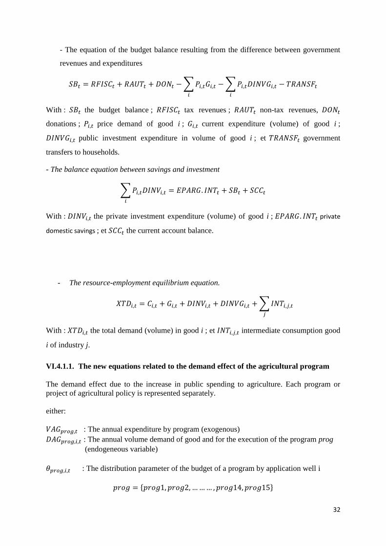
- The equation of the budget balance resulting from the difference between government

revenues and expenditures

𝑆𝐵𝑡 = 𝑅𝐹𝐼𝑆𝐶𝑡 + 𝑅𝐴𝑈𝑇𝑡 + 𝐷𝑂𝑁𝑡 − ∑ 𝑃𝑖,𝑡𝐺𝑖,𝑡

𝑖

− ∑ 𝑃𝑖,𝑡𝐷𝐼𝑁𝑉𝐺𝑖,𝑡

𝑖

− 𝑇𝑅𝐴𝑁𝑆𝐹𝑡

With : 𝑆𝐵𝑡 the budget balance ; 𝑅𝐹𝐼𝑆𝐶𝑡 tax revenues ; 𝑅𝐴𝑈𝑇𝑡 non-tax revenues, 𝐷𝑂𝑁𝑡

donations ; 𝑃𝑖,𝑡 price demand of good i ; 𝐺𝑖,𝑡 current expenditure (volume) of good i ;

𝐷𝐼𝑁𝑉𝐺𝑖,𝑡 public investment expenditure in volume of good i ; et 𝑇𝑅𝐴𝑁𝑆𝐹𝑡 government

transfers to households.

- The balance equation between savings and investment

∑ 𝑃𝑖,𝑡𝐷𝐼𝑁𝑉𝑖,𝑡

𝑖

= 𝐸𝑃𝐴𝑅𝐺. 𝐼𝑁𝑇𝑡 + 𝑆𝐵𝑡 + 𝑆𝐶𝐶𝑡

With : 𝐷𝐼𝑁𝑉𝑖,𝑡 the private investment expenditure (volume) of good i ; 𝐸𝑃𝐴𝑅𝐺. 𝐼𝑁𝑇𝑡 private

domestic savings ; et 𝑆𝐶𝐶𝑡 the current account balance.

- The resource-employment equilibrium equation.

𝑋𝑇𝐷𝑖,𝑡 = 𝐶𝑖,𝑡 + 𝐺𝑖,𝑡 + 𝐷𝐼𝑁𝑉𝑖,𝑡 + 𝐷𝐼𝑁𝑉𝐺𝑖,𝑡 + ∑ 𝐼𝑁𝑇𝑖,𝑗,𝑡

𝑗

With : 𝑋𝑇𝐷𝑖,𝑡 the total demand (volume) in good i ; et 𝐼𝑁𝑇𝑖,𝑗,𝑡 intermediate consumption good

i of industry j.

VI.4.1.1. The new equations related to the demand effect of the agricultural program

The demand effect due to the increase in public spending to agriculture. Each program or

project of agricultural policy is represented separately.

either:

𝑉𝐴𝐺𝑝𝑟𝑜𝑔,𝑡 : The annual expenditure by program (exogenous)

𝐷𝐴𝐺𝑝𝑟𝑜𝑔,𝑖,𝑡 : The annual volume demand of good and for the execution of the program prog

(endogeneous variable)

𝜃𝑝𝑟𝑜𝑔,𝑖,𝑡 : The distribution parameter of the budget of a program by application well i

𝑝𝑟𝑜𝑔 = {𝑝𝑟𝑜𝑔1, 𝑝𝑟𝑜𝑔2, … … … , 𝑝𝑟𝑜𝑔14, 𝑝𝑟𝑜𝑔15}

33

Thus, the annual volume demand of good i for the execution of the program is linked to the

annual cost of the program as follows:

𝑃𝑖,𝑡𝐷𝐴𝐺𝑝𝑟𝑜𝑔,𝑖,𝑡 = 𝜃𝑝𝑟𝑜𝑔,𝑖,𝑡𝑉𝐴𝐺𝑝𝑟𝑜𝑔,𝑡

This new demand results in a change in the resource- employment equilibrium equation:

𝑋𝑇𝐷𝑖,𝑡 = 𝐶𝑖,𝑡 + 𝐺𝑖,𝑡 + 𝐷𝐼𝑁𝑉𝑖,𝑡 + 𝐷𝐼𝑁𝑉𝐺𝑖,𝑡 + ∑ 𝐼𝑁𝑇𝑖,𝑗,𝑡

𝑗

+ ∑ 𝐷𝐴𝐺𝑝𝑟𝑜𝑔,𝑖,𝑡

𝑝𝑟𝑜𝑔

The budget balance is also altered in this way:

𝑆𝐵𝑡 = 𝑅𝐹𝐼𝑆𝐶𝑡 + 𝑅𝐴𝑈𝑇𝑡 + 𝐷𝑂𝑁𝑡 − ∑ 𝑃𝑖,𝑡𝐺𝑖,𝑡

𝑖

− ∑ 𝑃𝑖,𝑡𝐷𝐼𝑁𝑉𝐺𝑖,𝑡

𝑖

− 𝑇𝑅𝐴𝑁𝑆𝐹𝑡 − ∑ 𝑉𝐴𝐺𝑝𝑟𝑜𝑔,𝑡

𝑝𝑟𝑜𝑔

VI.4.1.1.1. If the expenditure is in substitution for other expenses

If the expenses of the agricultural program are substituting other expenses, while the same

amount should be subtracted from the other common items of expenditure or capital

expenditure. To do this, the budget deficit should be fixed (or exogenous) and an expenditure

becomes endogenous stations to be able to adjust.

VI.4.1.1.2. If the expenses are in addition to other expenses

If the expenses of the agricultural program are in addition to other expenses, results may vary,

according to the four options below:

• if financed by an increase in tax revenue, while the fiscal balance remains exogenous as well

as all other income and expenditure. Thus, only the tax revenue will have to adjust;

• if they are funded by donations, while the deficit remains exogenous and proxy donations

becomes endogenous;

• if they are financed by domestic borrowing, while the deficit is deteriorating while the

current account balance is exogenous. In this case, the stock of domestic debt increases;

• if they are financed by external debt, while the deficit is deteriorating but the current account

balance becomes endogenous, while domestic savings is fixed. In this case, the stock of

external debt also increases.

VI.4.2. Supply effects

34

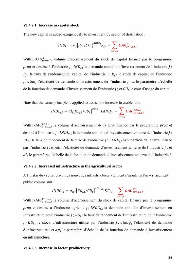
VI.4.2.1. Increase in capital stock

The new capital is added exogenously to investment by sector of destination :

𝐼𝑁𝐷𝑗,𝑡 = 𝛼𝑗[𝑅𝑗,𝑡/𝐶𝑈𝑡]𝜎𝑖𝑛𝑑𝑗

𝐾𝑗,𝑡 + ∑ 𝑂𝐴𝐺𝑝𝑟𝑜𝑔,𝑗,𝑡𝐾

𝑝𝑟𝑜𝑔

With : 𝑂𝐴𝐺𝑝𝑟𝑜𝑔,𝑗,𝑡𝐾 volume d’accroissement du stock de capital financé par le programme

prog et destiné à l’industrie j ; 𝐼𝑁𝐷𝑗,𝑡 la demande annuelle d’investissement de l’industrie j ;

𝑅𝑗,𝑡 le taux de rendement du capital de l’industrie j ; 𝐾𝑗,𝑡 le stock de capital de l’industrie

j ; 𝜎𝑖𝑛𝑑𝑗 l’élasticité de demande d’investissement de l’industrie j ; 𝛼𝑗 le paramètre d’échelle

de la fonction de demande d’investissement de l’industrie j ; et 𝐶𝑈𝑡 le cout d’usage du capital.

Note that the same principle is applied to assess the increase in arable land:

𝐼𝑁𝐷𝐿𝑗,𝑡 = 𝛼𝑙𝑗[𝑅𝐿𝑗,𝑡/𝐶𝑈𝑡]𝜎𝑖𝑛𝑑𝑙𝑗

𝐿𝐴𝑁𝐷𝑗,𝑡 + ∑ 𝑂𝐴𝐺𝑝𝑟𝑜𝑔,𝑗,𝑡𝐿𝐴𝑁𝐷

𝑝𝑟𝑜𝑔

With : 𝑂𝐴𝐺𝑝𝑟𝑜𝑔,𝑗,𝑡𝐿𝐴𝑁𝐷 le volume d’accroissement de la terre financé par le programme prog et

destiné à l’industrie j ; 𝐼𝑁𝐷𝐿𝑗,𝑡 la demande annuelle d’investissement en terre de l’industrie j ;

𝑅𝐿𝑗,𝑡 le taux de rendement de la terre de l’industrie j : 𝐿𝐴𝑁𝐷𝑗,𝑡 la superficie de la terre utilisée

par l’industrie j ; 𝜎𝑖𝑛𝑑𝑙𝑗 l’élasticité de demande d’investissement en terre de l’industrie j ; et

𝛼𝑙𝑗 le paramètre d’échelle de la fonction de demande d’investissement en terre de l’industrie j.

VI.4.2.2. Increased infrastructure in the agricultural sector

A l’instar du capital privé, les nouvelles infrastructures viennent s’ajouter à l’investissement

public comme suit :

𝐼𝑁𝐷𝐺𝑗,𝑡 = 𝛼𝑔𝑗[𝑅𝐺𝑗,𝑡/𝐶𝑈𝑡]𝜎𝑖𝑛𝑑𝑔𝑗

𝐾𝐺𝑗,𝑡 + ∑ 𝑂𝐴𝐺𝑝𝑟𝑜𝑔,𝑗,𝑡𝐾𝐺

𝑝𝑟𝑜𝑔

With : 𝑂𝐴𝐺𝑝𝑟𝑜𝑔,𝑗,𝑡𝐶𝐴𝑃𝑈𝐵 le volume d’accroissement du stock de capital financé par le programme

prog et destiné à l’industrie agricole j ; 𝐼𝑁𝐷𝐺𝑗,𝑡 la demande annuelle d’investissement en

infrastructure pour l’industrie j ; 𝑅𝐺𝑗,𝑡 le taux de rendement de l’infrastructure pour l’industrie

j ; 𝐾𝐺𝑗,𝑡 le stock d’infrastructure utilisé par l’industrie j ; 𝜎𝑖𝑛𝑑𝑔𝑗 l’élasticité de demande

d’infrastructure ; et 𝛼𝑔𝑗 le paramètre d’échelle de la fonction de demande d’investissement

en infrastructure.

VI.4.2.3. Increase in factor productivity

35

It is difficult to measure the effects of growth policy factor productivity, since they act

indirectly on production. Moreover, the literature is somewhat verbose about it. However, the

assumption made in this exercise is that on a given time horizon, the present value of the

increase in productivity is the amount invested today. In other words, it can be admitted that

the government hopes to increase long-term productivity of the same amount injected today as

part of its policy. Thus, using the factor demand functions, the effect of increase in

productivity can be considered as follows:

- Increased labor productivity

𝑉𝐴𝑗 = 𝐴𝑗𝐾𝑇𝑗,𝑡𝛼𝑘 [(1 + ∑ 𝑂𝐴𝐺𝑝𝑟𝑜𝑔,𝑗,𝑡

𝑃𝑅𝐷_𝐿𝐷

𝑝𝑟𝑜𝑔

) 𝐿𝐷𝑗,𝑡]

𝛼𝑣𝑗

With : 𝑂𝐴𝐺𝑝𝑟𝑜𝑔,𝑗,𝑡𝑃𝑅𝐷_𝐿𝐷 l’augmentation (en pourcentage de la demande initiale de travail) de la

productivité du travail financée par le programme prog et destinée à l’industrie agricole j ;

𝐿𝐷𝑗,𝑡 la demande de travail de l’industrie j ; 𝑃𝑉𝐴𝑗 le prix de la valeur ajoutée de l’industrie j ;

𝑉𝐴𝑗 le volume de la valeur ajoutée de l’industrie j ; 𝑊𝑗,𝑡 le taux de salaire payé par l’industrie

j ; et 𝛼𝑣𝑗 la part de la demande de travail sur la valeur ajoutée.

- Increase the productivity of capital

𝐾𝑃𝑗 = 𝐴𝑗 [(1 + ∑ 𝑂𝐴𝐺𝑝𝑟𝑜𝑔,𝑗,𝑡𝑃𝑅𝐷_𝐾

𝑝𝑟𝑜𝑔

) 𝐾𝑗,𝑡]

𝛼𝑘𝑗

𝐿𝐴𝑁𝐷𝑗,𝑡

(1−𝛼𝑘𝑗)

With : 𝑂𝐴𝐺𝑝𝑟𝑜𝑔,𝑗,𝑡𝑃𝑅𝐷_𝐾 l’augmentation (en pourcentage de la demande initiale d’équipement) de

la productivité du capital financée par le programme prog et destinée à l’industrie agricole

j ; 𝐾𝑗,𝑡 le stock de capital (équipement) de l’industrie j ; 𝑅𝑃𝑗 le rendement du capital

(équipement et terre) ; 𝐾𝑃𝑗 le stock de capital (équipement et terre) ; 𝑅𝑗,𝑡 le rendement du

capital (équipement) ; et 𝛼𝑘𝑗 la part du stock capital (équipement) sur le stock total de capital

(équipement, terre) de l’industrie j.

- Increased productivity of land

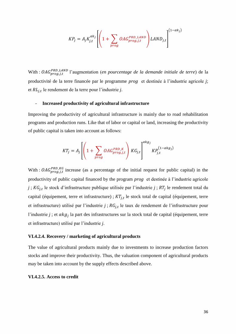
36

𝐾𝑃𝑗 = 𝐴𝑗𝐾𝑗,𝑡

𝛼𝑘𝑗 [(1 + ∑ 𝑂𝐴𝐺𝑝𝑟𝑜𝑔,𝑗,𝑡𝑃𝑅𝐷_𝐿𝐴𝑁𝐷

𝑝𝑟𝑜𝑔

) 𝐿𝐴𝑁𝐷𝑗,𝑡]

(1−𝛼𝑘𝑗)

With : 𝑂𝐴𝐺𝑝𝑟𝑜𝑔,𝑗,𝑡𝑃𝑅𝐷_𝐿𝐴𝑁𝐷 l’augmentation (en pourcentage de la demande initiale de terre) de la

productivité de la terre financée par le programme prog et destinée à l’industrie agricole j;

et 𝑅𝐿𝑗,𝑡 le rendement de la terre pour l’industrie j.

- Increased productivity of agricultural infrastructure

Improving the productivity of agricultural infrastructure is mainly due to road rehabilitation

programs and production runs. Like that of labor or capital or land, increasing the productivity

of public capital is taken into account as follows:

𝐾𝑇𝑗 = 𝐴𝑗 [(1 + ∑ 𝑂𝐴𝐺𝑝𝑟𝑜𝑔,𝑗,𝑡𝑃𝑅𝐷_𝐾

𝑝𝑟𝑜𝑔

) 𝐾𝐺𝑗,𝑡]

𝛼𝑘𝑔𝑗

𝐾𝑃𝑗,𝑡

(1−𝛼𝑘𝑔𝑗)

With : 𝑂𝐴𝐺𝑝𝑟𝑜𝑔,𝑗,𝑡𝑃𝑅𝐷_𝐾𝐺 increase (as a percentage of the initial request for public capital) in the

productivity of public capital financed by the program prog et destinée à l’industrie agricole

j ; 𝐾𝐺𝑗,𝑡 le stock d’infrastructure publique utilisée par l’industrie j ; 𝑅𝑇𝑗 le rendement total du

capital (équipement, terre et infrastructure) ; 𝐾𝑇𝑗,𝑡 le stock total de capital (équipement, terre

et infrastructure) utilisé par l’industrie j ; 𝑅𝐺𝑗,𝑡 le taux de rendement de l’infrastructure pour

l’industrie j ; et 𝛼𝑘𝑔𝑗 la part des infrastructures sur la stock total de capital (équipement, terre

et infrastructure) utilisé par l’industrie j.

VI.4.2.4. Recovery / marketing of agricultural products

The value of agricultural products mainly due to investments to increase production factors

stocks and improve their productivity. Thus, the valuation component of agricultural products

may be taken into account by the supply effects described above.

VI.4.2.5. Access to credit

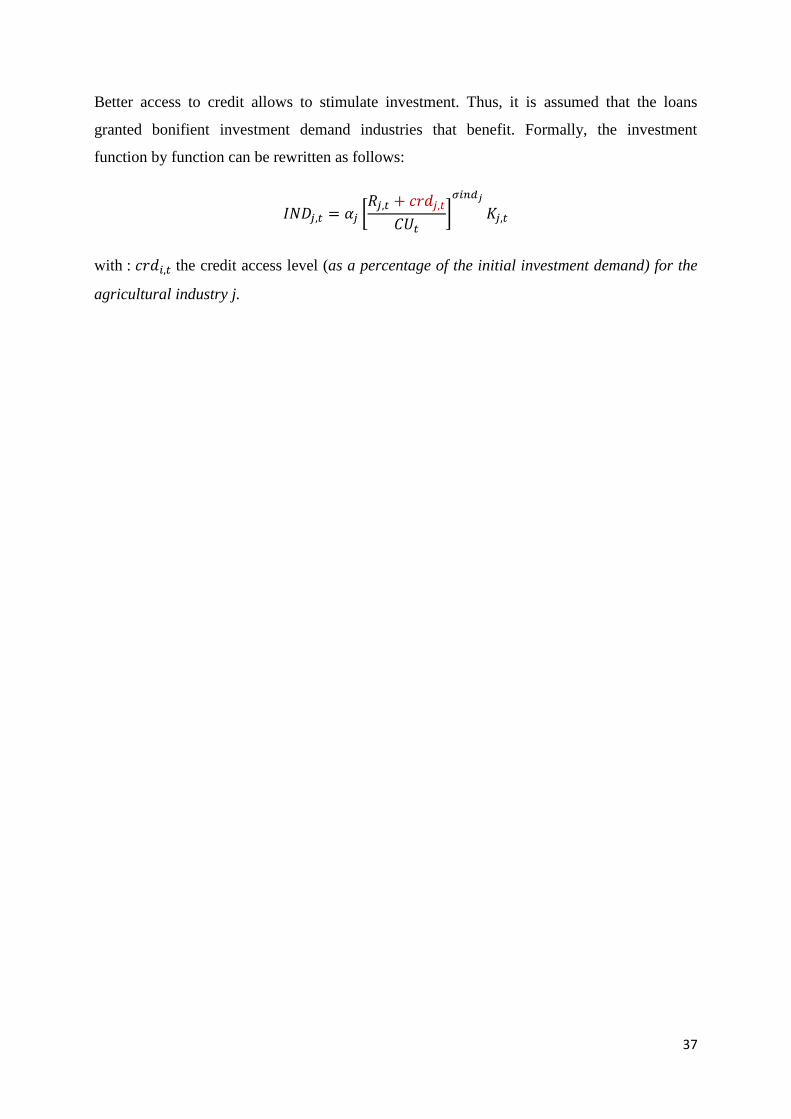
37

Better access to credit allows to stimulate investment. Thus, it is assumed that the loans

granted bonifient investment demand industries that benefit. Formally, the investment

function by function can be rewritten as follows:

𝐼𝑁𝐷𝑗,𝑡 = 𝛼𝑗 [𝑅𝑗,𝑡 + 𝑐𝑟𝑑𝑗,𝑡

𝐶𝑈𝑡]

𝜎𝑖𝑛𝑑𝑗

𝐾𝑗,𝑡

with : 𝑐𝑟𝑑𝑖,𝑡 the credit access level (as a percentage of the initial investment demand) for the

agricultural industry j.

38

VII. RESULTS AND INTERPRETATION

VII.1. Demand effects of expenditure agricultural policy

The analyzed results below outline the short-term macroeconomic effects from financing modes

additional agricultural spending PICTs (2013-2015). This exercise seems essential although Table III.1

has the sources of financing. The reason is that in considering the principle of fungibility of budgetary

resources, it may be unrealistic to expect, for example, that the contributions of donors necessarily in

addition to existing expenditures. Indeed, portfolio constraints can bring a landlord to increase its

agricultural funding and reduce other types of financing. In this case, additional agricultural spending

would be to replace other budget expenditures.

The following tables show how the results can be different depending implementing fiscal policy.

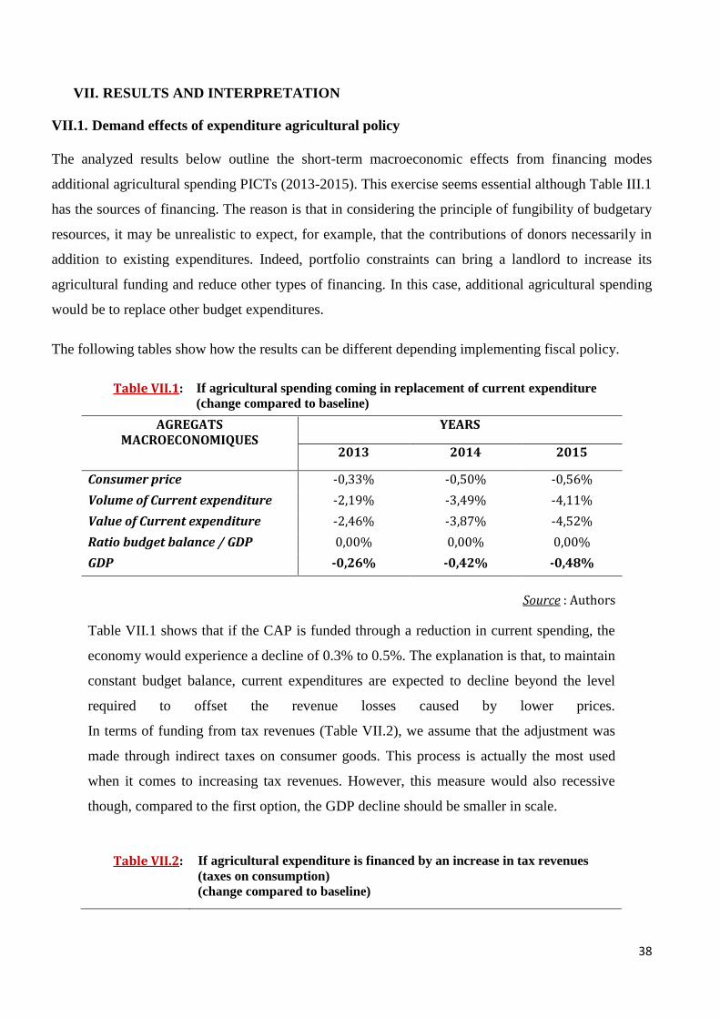
Table VII.1:

If agricultural spending coming in replacement of current expenditure

(change compared to baseline)

AGREGATS MACROECONOMIQUES

YEARS

2013 2014 2015

Consumer price -0,33% -0,50% -0,56%

Volume of Current expenditure -2,19% -3,49% -4,11%

Value of Current expenditure -2,46% -3,87% -4,52%

Ratio budget balance / GDP 0,00% 0,00% 0,00%

GDP -0,26% -0,42% -0,48%

Source : Authors

Table VII.1 shows that if the CAP is funded through a reduction in current spending, the

economy would experience a decline of 0.3% to 0.5%. The explanation is that, to maintain

constant budget balance, current expenditures are expected to decline beyond the level

required to offset the revenue losses caused by lower prices.

In terms of funding from tax revenues (Table VII.2), we assume that the adjustment was

made through indirect taxes on consumer goods. This process is actually the most used

when it comes to increasing tax revenues. However, this measure would also recessive

though, compared to the first option, the GDP decline should be smaller in scale.

Table VII.2:

If agricultural expenditure is financed by an increase in tax revenues

(taxes on consumption)

(change compared to baseline)

39

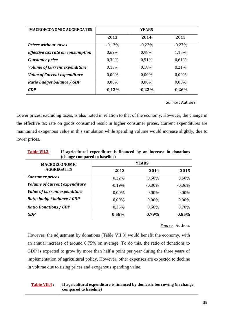
MACROECONOMIC AGGREGATES YEARS

2013 2014 2015

Prices without taxes -0,13% -0,22% -0,27%

Effective tax rate on consumption 0,62% 0,98% 1,15%

Consumer price 0,30% 0,51% 0,61%

Volume of Current expenditure 0,13% 0,18% 0,21%

Value of Current expenditure 0,00% 0,00% 0,00%

Ratio budget balance / GDP 0,00% 0,00% 0,00%

GDP -0,12% -0,22% -0,26%

Source : Authors

Lower prices, excluding taxes, is also noted in relation to that of the economy. However, the change in

the effective tax rate on goods consumed result in higher consumer prices. Current expenditures are

maintained exogenous value in this simulation while spending volume would increase slightly, due to

lower prices.

Table VII.3 :

If agricultural expenditure is financed by an increase in donations

(change compared to baseline)

MACROECONOMIC AGGREGATES

YEARS

2013 2014 2015

Consumer prices 0,32% 0,50% 0,60%

Volume of Current expenditure -0,19% -0,30% -0,36%

Value of Current expenditure 0,00% 0,00% 0,00%

Ratio budget balance / GDP 0,00% 0,00% 0,00%

Ratio Donations / GDP 0,35% 0,58% 0,70%

GDP 0,58% 0,79% 0,85%

Source : Authors

However, the adjustment by donations (Table VII.3) would benefit the economy, with

an annual increase of around 0.75% on average. To do this, the ratio of donations to

GDP is expected to grow by more than half a point per year during the three years of

implementation of agricultural policy. However, other expenses are expected to decline

in volume due to rising prices and exogenous spending value.

Table VII.4 : If agricultural expenditure is financed by domestic borrowing (in change

compared to baseline)

40

MACROECONOMIC AGGREGATES YEARS

2013 2014 2015

Consumer prices 0,00% 0,10% 0,25%

Volume of Current expenditure 0,00% -0,05% -0,12%

Value Current expenditure 0,00% 0,00% 0,00%

Ratio budget balance / GDP -0,50% -0,85% -1,10%

Private Investment -2,94% -5,14% -6,82%

GDP 0,00% -0,19% -0,51%

Source : Authors

If the additional agricultural expenditure is financed by domestic savings (Table VII.4), it would

follow a systematic deterioration of the fiscal balance. Private investment also suffer a simultaneous

decrease if part of domestic savings by households and businesses is transferred to the public sector.

Thus, the option of financing by domestic borrowing would result in a contraction in activity and

higher public debt.

Table VII.5 :

If agricultural expenditure is financed by external borrowing

(change compared to baseline)

MACROECONOMIC AGGREGATES YEARS

2013 2014 2015

Consumer prices 0,28% 0,47% 0,58%

Volume of Current expenditure -0,17% -0,28% -0,35%

Value Current expenditure 0,00% 0,00% 0,00%

Ratio budget balance / GDP -0,37% -0,60% -0,73%

Ratio of current account / GDP -0,31% -0,53% -0,65%

GDP 0,51% 0,70% 0,75%

Source : Authors

Regarding external debt financing (Table VII.5), it would cause a simultaneous deterioration in the

budget balance and the current balance. At the same time, an increase in GDP and a slight inflationary

pressure would be noted.

41

In general, the effectiveness of the impact demand from increased agricultural investment is not

necessarily guaranteed, and depends heavily on financing options. The use of internal financing

(alternative spending, domestic tax or loan) is just a way to transfer the request of the public or private

sector to the public sector. By cons, funding based on a combination of grants and external borrowing

would cause a positive reaction in activity, despite a slight pressure on prices.

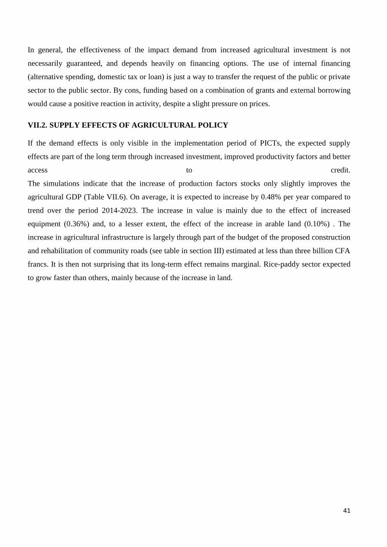
VII.2. SUPPLY EFFECTS OF AGRICULTURAL POLICY

If the demand effects is only visible in the implementation period of PICTs, the expected supply

effects are part of the long term through increased investment, improved productivity factors and better

access to credit.

The simulations indicate that the increase of production factors stocks only slightly improves the

agricultural GDP (Table VII.6). On average, it is expected to increase by 0.48% per year compared to

trend over the period 2014-2023. The increase in value is mainly due to the effect of increased

equipment (0.36%) and, to a lesser extent, the effect of the increase in arable land (0.10%) . The

increase in agricultural infrastructure is largely through part of the budget of the proposed construction

and rehabilitation of community roads (see table in section III) estimated at less than three billion CFA

francs. It is then not surprising that its long-term effect remains marginal. Rice-paddy sector expected

to grow faster than others, mainly because of the increase in land.

42

Table VII.6: Effects of increased capital stock value added agricultural sectors (on average over the period 2014-2023)

the effects are measured by change from the baseline

Effet de l'accroissement du stock du facteur :

AGRICULTURE maize rice

paddy millet

other agr. viv.

groundnut

cotton tomato sugar cane

autres agr. ind.

Equipment 0,36% 0,39% 0,39% 0,27% 0,39% 0,29% 0,20% 0,48% 0,20% 0,58%

Land 0,10% 0,07% 0,39% 0,05% 0,07% 0,05% 0,03% 0,08% 0,03% 0,10%

Infrastructures 0,03% 0,03% 0,03% 0,02% 0,03% 0,02% 0,02% 0,03% 0,02% 0,04%

TOTAL EFFECT 0,48% 0,49% 0,81% 0,34% 0,48% 0,37% 0,26% 0,60% 0,26% 0,72%

Source : Authors

Table VII.7: Effects of increased productivity on the added value of the agricultural sector (on average over the period 2014-2023)

the effects are measured by change from the baseline

Effect of the increase in the productivity of factors :

AGRICULTURE maize rice

paddy millet

other agr. viv.

groundnut

cotton tomato sugar cane

autres agr. ind.

Labor 1,79% 2,06% 1,60% 1,39% 2,02% 1,46% 0,94% 2,48% 0,95% 3,02%

Equipment 0,20% 0,22% 0,17% 0,15% 0,22% 0,16% 0,10% 0,27% 0,11% 0,33%

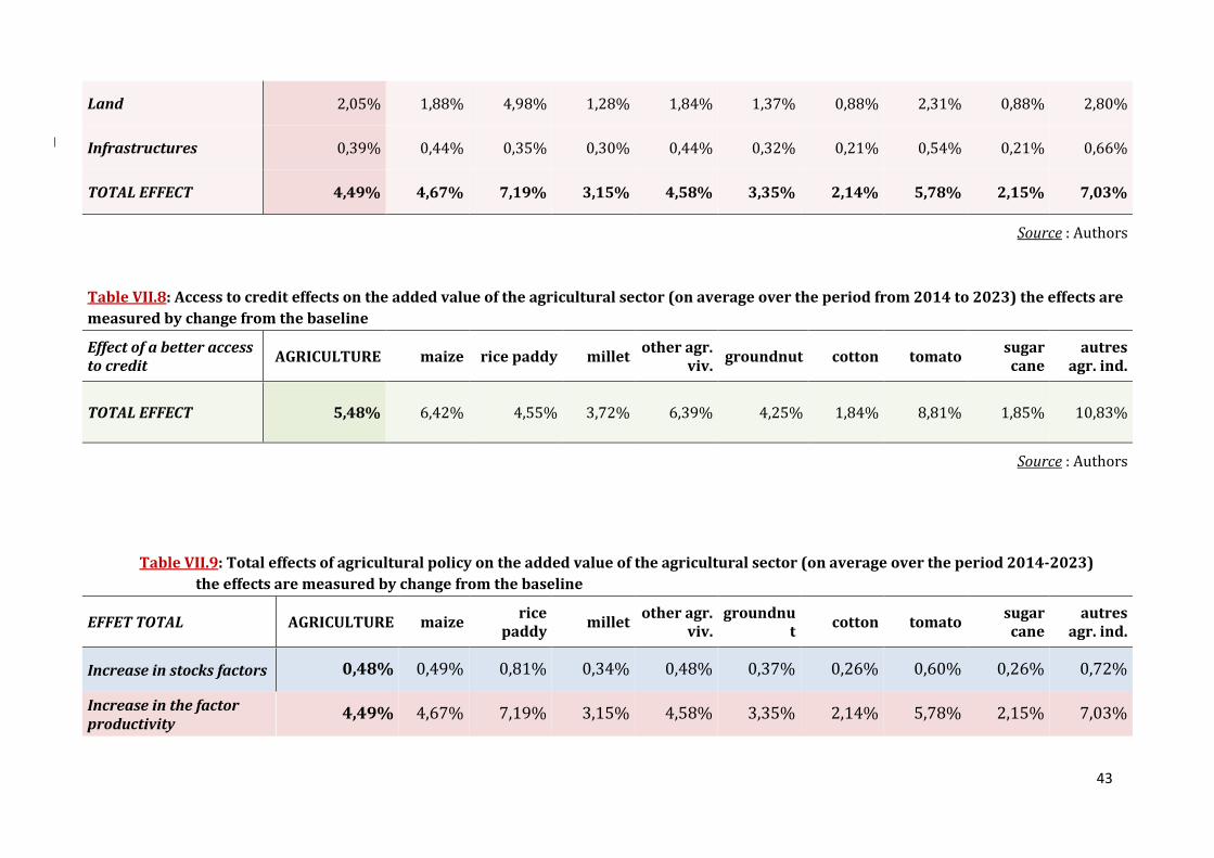
43

Land 2,05% 1,88% 4,98% 1,28% 1,84% 1,37% 0,88% 2,31% 0,88% 2,80%

Infrastructures 0,39% 0,44% 0,35% 0,30% 0,44% 0,32% 0,21% 0,54% 0,21% 0,66%

TOTAL EFFECT 4,49% 4,67% 7,19% 3,15% 4,58% 3,35% 2,14% 5,78% 2,15% 7,03%

Source : Authors

Table VII.8: Access to credit effects on the added value of the agricultural sector (on average over the period from 2014 to 2023) the effects are

measured by change from the baseline

Effect of a better access to credit

AGRICULTURE maize rice paddy millet other agr.

viv. groundnut cotton tomato

sugar cane

autres agr. ind.

TOTAL EFFECT 5,48% 6,42% 4,55% 3,72% 6,39% 4,25% 1,84% 8,81% 1,85% 10,83%

Source : Authors

Table VII.9: Total effects of agricultural policy on the added value of the agricultural sector (on average over the period 2014-2023)

the effects are measured by change from the baseline

EFFET TOTAL AGRICULTURE maize rice

paddy millet

other agr. viv.

groundnut

cotton tomato sugar cane

autres agr. ind.

Increase in stocks factors 0,48% 0,49% 0,81% 0,34% 0,48% 0,37% 0,26% 0,60% 0,26% 0,72%

Increase in the factor productivity

4,49% 4,67% 7,19% 3,15% 4,58% 3,35% 2,14% 5,78% 2,15% 7,03%

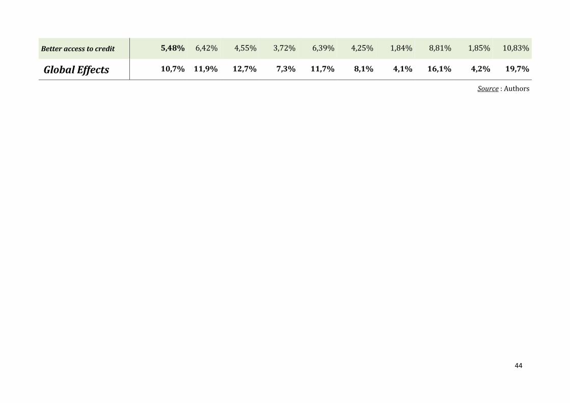
44

Better access to credit 5,48% 6,42% 4,55% 3,72% 6,39% 4,25% 1,84% 8,81% 1,85% 10,83%

Global Effects 10,7% 11,9% 12,7% 7,3% 11,7% 8,1% 4,1% 16,1% 4,2% 19,7%

Source : Authors

45

46

The weakness of the effects of the increase in capital stock is explained by the fact that they cause,

simultaneously, reduced workload. Indeed, the increase in these stocks leads to rise in the relative

price of labor, reducing its request. This substitution effect reduces the expected effect of the

increase in stocks factors.

As for the investment in improving productivity, they are expected to generate, on average, an

increase of 4.49% per annum of agricultural value added (Table VII.7). The productivity of the

land contributes significantly to 2.05%, mainly because of the recovery of the seed capital

programs and rehabilitation of irrigation schemes. Improving labor productivity also seems to give

good results (1.79% of agricultural GDP) due to additional investments CFAF 34 billion spread

across several programs.

Finally, investments through better access to credit can generate an annual increase of 5.48% of

agricultural GDP and appear more productive than previously simulated. This performance can be

explained by the simple fact that the strengthening of the guarantee system of rural credit by the

State reduces the user cost of capital, which promotes, in turn, investment to agriculture. However,

from a macroeconomic perspective, such performance is to qualify when the incentive to invest in

agriculture suggests disinvestment in other sectors of the economy.

GraphVII.1: Decomposition of the annual change in agricultural GDP

Source : Authors

GraphVII.2 : Annual change in GDP

0%

2%

4%

6%

8%

10%

12%

14%

2014 2015 2016 2017 2018 2019 2020 2021 2022 2023

Effet Augmentation des stocks de facteursEffet Accès au créditEffet Augmentation de la porductivité

Productivity Stocks Credit

47

Source : Authors

Overall, the new direction of agricultural policy, implemented through the PICTs, should generate

an average annual increase of 10.7% of agricultural GDP. VII.1 The graph shows the growth

dynamics of agricultural GDP between 2014 and 2023, with a breakdown of the different supply

effects. The graph shows a gradual increase in production during the first years of agricultural

policy is implemented. Mature, investments continue to boost production, but lose more and more

effective, due to their depreciation over time. Consequently, agricultural policy should stimulate

economic activity and allow the GDP to increase by 1% on average relative to trend.

GraphVII.3 : Change in ratio of imports to GDP

Source : Authors

Furthermore, the economic performance raised by agricultural policy should help reduce imports

(Figure VII.3). This reduction is made possible by the import substitution of agricultural products

and other food products present in the secondary sector. The decrease in the ratio of imports to

GDP would be maintained in the long term, due to the sustained increase in economic activity.

0.0%

0.2%

0.4%

0.6%

0.8%

1.0%

1.2%

1.4%

1.6%

2014 2015 2016 2017 2018 2019 2020 2021 2022 2023

-1.4%

-1.2%

-1.0%

-0.8%

-0.6%

-0.4%

-0.2%

0.0%

2014 2015 2016 2017 2018 2019 2020 2021 2022 2023

48

VII.3. THE RISK FACTORS RELATED TO THE AGRICULTURAL POLICY

The expected results of the agricultural policy, presented above, are obtained under the

assumption of efficiency in the use of capital expenditure. In other words, the goal of the state,

expressed through an increase of 126 billion FCFA of agricultural expenditure, provides a

sustained increase of nearly 11% of the agricultural activity. This can then form the optimistic

scenario of the study.

However, the occurrence of risks related to the implementation of programs is not ruled out.

Potential risks that moderate efficiency of expenditures are numerous, but can be summarized in

two main points. First, it is likely that some of the planned investments will not reach its

destination, and second, it is possible that the process of monitoring and maintenance of

investments is faulty.

VII.3.1. Decrease in the volume and effectiveness of planned investments

The finding of non-effectiveness of agricultural public investment is real and many reasons help

explain this phenomenon. The Public Expenditure in the agricultural sector highlighted the many

pitfalls related to the effective implementation of agricultural investments.

On the one hand, the institutional framework remains relatively weak due to the many institutions

involved in the sector, and which are subject to constant changes in their organization and

functions.

Moreover, almost all of the projects are strained through technical failures noted in the selection

process and project / program preparation, budget preparation, budget execution and budget

monitoring. These difficulties are inefficiencies in the allocation of budgetary resources and

reducing the volume and performance of agricultural investments.

Moreover, there is a relatively large gap between the allocated expenses and those executed.

Based on the review of agricultural expenditure, the rate of implementation of agricultural

investments stood at 80% on average between 2005 and 2010.

For all these reasons, it is desirable to perform simulations that take into account the possibility of

non-effective or not effective spending. To do this, we assume that the non-effective investments

are between 20% and 40% of planned investments.

GraphVII.4: Annual change in agricultural GDP with a loss of efficiency between 20% and 40%

49

Source : Authors

In this case, the graph VII.4 shows that the increase of agricultural GDP is significantly lower than

referring to completely expenditures made (red curve). The annual difference could be between 3

and 5 percentage points. The lack of effectiveness of agricultural investments would increase

agricultural GDP between 6.2% and 8.5% on average over the period 2014-2023. The GDP

growth would be between 0.6% and 0.9% on average.

VII.3.2. Failure of the monitoring system, maintenance and maintenance investments

When monitoring, servicing and maintenance is not properly in place, the tangible and

intangible investments depreciate faster than expected. In particular, an accelerated

reduction in the yield of physical factors stocks can be seen due to their premature

deterioration. In addition, investments oriented towards increasing the productivity of

factors can not be effective if the desired level is not maintained after the

implementation phase. Finally, poor management of agricultural credit guarantee fund

may result in a significant number of problem loans and non-repayments that jeopardize

2%

4%

6%

8%

10%

12%

14%

2014 2015 2016 2017 2018 2019 2020 2021 2022 2023

optimistic scenario

Loss of efficiency between 20% and 40%

50

the sustainability of the system.

Risk factors, mentioned above, is likely to lead to a rapid depreciation of public

investment. To assess the consequences of these risks, it can be assumed that the

depreciation is three to four times faster than in the optimistic scenario.

GraphVII.5: Annual change in agricultural GDP with a rapid depreciation of public investment

Source : Authors

The graph shows that the increase of agricultural GDP follows a different path from that of the

optimistic scenario. Thus, the investment value added effects disappear in an accelerated manner,

inducing a rapid return to trend situation. The change in agricultural value added could even

become negative in case of high depreciation. On average, the increase of agricultural GDP would

be between 5.7% and 7.4% over the analysis period. As for GDP, the increase would average

between 0.5% and 0.8%.

-2%

0%

2%

4%

6%

8%

10%

12%

14%

2014 2015 2016 2017 2018 2019 2020 2021 2022 2023

optimistic scenario

Rapid depreciation of investments

51

VIII. CONCLUSION

For decades, senegalese agriculture has experienced many difficulties related to low factor

productivity and highly fluctuating production. Consequently, it has less and less participated in

the creation of national wealth, causing suddenly a massive migration from rural to urban areas.

This study investigated whether the new strategic directions of the Government's agricultural

policy are likely to stimulate a real momentum for change in the industry. In particular, the study

focused on new projects and programs written in the PICTs whose fiscal cost is estimated at just

over 126 billion FCFA.

The stylized facts highlighted the fact that in addition to its high volatility, the contribution of

agriculture to the GDP has declined significantly over the last fifteen years. Indeed, the share of

agriculture in GDP has decreased from 10.10% between 1997 and 2001 to 7.86% between 2007

and 2011. This modest contribution to GDP, associated with significant weight of labor ( nearly

30% of the working population), gives fairly accurate indication of the low productivity of

agricultural labor which is five times less than the non-agricultural sector one. The agricultural

sector's difficulties are linked in particular to the obsolescence of agricultural equipment, the

degradation of infrastructure, seed quality, lack of storage units and inadequate agricultural credit.

As a result, the output gap remains critical, resulting in a high level of imports of agricultural

products.

A general equilibrium model integrating the agricultural sector, was used to measure the short-

term effects (demand effects) and those of long term (supply effect) of new agricultural projects

and programs.

The results show that the effectiveness of the demand effect resulting from the increase in public

spending agricultural investment, is not necessarily guaranteed, but depends mainly on financing

options. The use of internal financing (alternative spending, domestic tax or loan) is just a way to

transfer the request of the public or private sector to the public sector. By cons, funding based on a

combination of grants and external borrowing would cause a positive reaction in activity, despite a

slight pressure on prices.

If the effects application is only visible during the period of the investment's implementation, the

expected supply effects are part of the long term through increased physical capital, improvements

in factor productivity and better access to credit. The supply effects therefore entail a change in

farm production function.

The simulations indicate that the increase of production factors stocks would improve slightly the

agricultural GDP. On average, it is expected to increase by 0.48% per year compared to trend over

52

the period 2014-2023. The weakness of the effects of the increase in capital stock is explained by

the fact that these physical investments simultaneously cause a decrease in the volume of work,

the cost is relatively higher. However, investments in improving the productivity of factors are

expected to generate, on average, an increase of 4.49% per annum of the agricultural value added.

Finally, investments through better access to credit appear more productive, judging by the annual

increase of 5.48% of agricultural GDP they can generate.

Overall, the new direction of agricultural policy, implemented through the PICTs, should generate

an average annual increase of 10.7% of the agricultural activity over the period 2014-2023. This

increase corresponds to a gain of almost 1% of GDP per year. However, these results are obtained

under the assumption that capital expenditures are used effectively. Indeed, the occurrence of risks

related to the implementation of programs is not ruled out. First, it is assumed that the

implementation of agricultural investment is accompanied by losses in volume and efficiency.

These losses would bear the increase in agricultural GDP between 6.2% and 8.5% on average over

the period 2014-2023. The GDP growth would be between 0.6% and 0.9%. Secondly, it is likely

that failures are noted in the monitoring process, service and maintenance of investments. This

would result in accelerated depreciation of tangible and intangible investments. In this case, the

increase of agricultural GDP would be reduced between 5.7% and 7.4% over the analysis period.

As for the GDP growth rate would average between 0.5% and 0.8%.

53

Bibliographie

Antle J. M. (1983), "Infrastructure and Aggregate Agricultural Productivity: International

Evidence", Economic Development and Cultural Change Vol.31, N°3, PP.6-10.

Gisselquist R. A. R. (1999), " Geography and Agricultural Productivity in India : Implications for

Tamil Nadu", Harvard Institute for International Development

Dansokho M. (2000), "Essai de Simulation de L'ajustement Structurel dans le Sector Agricole au

Sénégal à l'aide d'un Modèle Calculable d'Equilibre Général (MEGC)", Thèse de Doctorat d'Etat

és Sciences Economiques, Université Cheikh Anta DIOP de Dakar.

Rozelle S., J. E. Taylor et A. deBrauw, (1999), "Migration, Remittances, and Agricultural

Productivity in China", The American Economic Review, Vol.89, N°2, Papers and Proceedings of

the One Hundred Eleventh Annual Meeting of The American Economic Association, PP.5-6.

Wiebe K. (2003), "Linking Land Quality, Agricultural Productivity, and Food Security", United

States Department of Agriculture, Economic Research Service, Agricultural Economic Report

Number 823, PP.19-26, 43-48.

Alston, Julian (2010), "The Benefits from Agricultural Research and Development, Innovation,

and Productivity Growth", OECD Food, Agriculture and Fisheries Papers, N°31, OECD

Publishing, PP.13-20.

Pauw K., J. Thurlow et R. Uaiene (2011), "Agricultural Growth and Poverty Reduction in

Mozambique: Technical Analysis in Support of the Comprehensive Africa Agriculture

Development Program (CAADP)", International Food Policy Research Institute (IFPRI) et

United Nations University - World Institute for Development Economics Research.

Kussa M. U. (2012), "Farmer’s Health and Agricultural Productivity in Rural Ethiopia",

Norwegian University of Life Sciences, UMB School of Economics and Business, Master Thesis,

PP.33.

Darku Malla et Tran (2012), "Stochastic Frontier Approach of Measuring Agricultural

Productivity & Efficiency : Accounting for Innovations", PP.7-8.

Thirtle, Colin et al (2001), "Relationship between changes in agricultural productivity and the

incidence of poverty in developing countries"

Diskin, Patrick. (1999), "Agricultural Productivity Indicators Measurement Guide", Food and

Nutrition Technical Assistance.

54

Ministère de l'économie et des finances (2012), " Programme Triennal d'Investissements Publics

(PTIP)", Direction de la Coopération Economique et Financière, PP.18-21.

Benkahla, Amel et Pape N. Dièye (2010), "Analyse des plans d’investissements agricoles : les

cas du Sénégal, du Mali et de la CEDEAO", Initiative Prospective Agricole et Rurale (IPAR).

Benkahla, Amel (2011), "Analyse du Plan National D’investissement dans le Sector Agricole du

Sénégal", Initiative Prospective Agricole et Rurale (IPAR).

Solow, Robert (1957), "Technical Change and the Aggregate Production Function ", PP.6.

Aka, François, François Joseph Cabral, Sylvie Da Sylva, Abdoulaye Diagne, Mohamadou

Lamine Dia, Ngolo Diarra, Mamadou Faye, Moussa Mbaye, Arona Niang, Malamine Sadio,

Ousseynou Sarr et Harouna Wassongma (2012), "Revue des dépenses publiques dans le sector

de l'agriculture", USAID, Ministère de l'agriculture du Sénégal, Banque Mondiale, CRES.

République du Sénégal (2008), "Revue des efforts de développement dans le sector agricole",

PP.6-8.