dense%vectors - stanford universityjurafsky/slp3/slides/vector2.pdf · singular vectors of the...
TRANSCRIPT

Vector Semantics
Dense Vectors
Dan Jurafsky
Sparse versus dense vectors
• PPMI vectors are• long (length |V|= 20,000 to 50,000)• sparse (most elements are zero)
• Alternative: learn vectors which are• short (length 200-‐1000)• dense (most elements are non-‐zero)
2
Dan Jurafsky
Sparse versus dense vectors
• Why dense vectors?• Short vectors may be easier to use as features in machine learning (less weights to tune)
• Dense vectors may generalize better than storing explicit counts• They may do better at capturing synonymy:• car and automobile are synonyms; but are represented as distinct dimensions; this fails to capture similarity between a word with car as a neighbor and a word with automobile as a neighbor
3

Dan Jurafsky
Three methods for getting short dense vectors
• Singular Value Decomposition (SVD)• A special case of this is called LSA – Latent Semantic Analysis
• “Neural Language Model”-‐inspired predictive models• skip-‐grams and CBOW
• Brown clustering
4

Vector Semantics
Dense Vectors via SVD

Dan Jurafsky
Intuition• Approximate an N-‐dimensional dataset using fewer dimensions• By first rotating the axes into a new space• In which the highest order dimension captures the most
variance in the original dataset• And the next dimension captures the next most variance, etc.• Many such (related) methods:
• PCA – principle components analysis• Factor Analysis• SVD
6

Dan Jurafsky
1 2 3 4 5 6
1
2
3
4
5
6
71 2 3 4 5 6
1
2
3
4
5
6
PCA dimension 1
PCA dimension 2
Dimensionality reduction

Dan Jurafsky
Singular Value Decomposition
8
Any rectangular w x c matrix X equals the product of 3 matrices:W: rows corresponding to original but m columns represents a dimension in a new latent space, such that
• M column vectors are orthogonal to each other• Columns are ordered by the amount of variance in the dataset each new dimension accounts for
S: diagonal m x mmatrix of singular values expressing the importance of each dimension.C: columns corresponding to original but m rows corresponding to singular values

Dan Jurafsky
Singular Value Decomposition
238 LANDAUER AND DUMAIS
Appendix
An Introduction to Singular Value Decomposition and an LSA Example
Singu la r Value D e c o m p o s i t i o n ( S V D )
A well-known proof in matrix algebra asserts that any rectangular matrix (X) is equal to the product of three other matrices (W, S, and C) of a particular form (see Berry, 1992, and Golub et al., 1981, for the basic math and computer algorithms of SVD). The first of these (W) has rows corresponding to the rows of the original, but has m columns corresponding to new, specially derived variables such that there is no correlation between any two columns; that is, each is linearly independent of the others, which means that no one can be constructed as a linear combination of others. Such derived variables are often called principal components, basis vectors, factors, or dimensions. The third matrix (C) has columns corresponding to the original columns, but m rows composed of derived singular vectors. The second matrix (S) is a diagonal matrix; that is, it is a square m × m matrix with nonzero entries only along one central diagonal. These are derived constants called singular values. Their role is to relate the scale of the factors in the first two matrices to each other. This relation is shown schematically in Figure A1. To keep the connection to the concrete applications of SVD in the main text clear, we have labeled the rows and columns words (w) and contexts (c) . The figure caption defines SVD more formally.
The fundamental proof of SVD shows that there always exists a decomposition of this form such that matrix mu!tiplication of the three derived matrices reproduces the original matrix exactly so long as there are enough factors, where enough is always less than or equal to the smaller of the number of rows or columns of the original matrix. The number actually needed, referred to as the rank of the matrix, depends on (or expresses) the intrinsic dimensionality of the data contained in the cells of the original matrix. Of critical importance for latent semantic analysis (LSA), if one or more factor is omitted (that is, if one or more singular values in the diagonal matrix along with the corresponding singular vectors of the other two matrices are deleted), the reconstruction is a least-squares best approximation to the original given the remaining dimensions. Thus, for example, after constructing an SVD, one can reduce the number of dimensions systematically by, for example, remov- ing those with the smallest effect on the sum-squared error of the approx- imation simply by deleting those with the smallest singular values.
The actual algorithms used to compute SVDs for large sparse matrices of the sort involved in LSA are rather sophisticated and are not described here. Suffice it to say that cookbook versions of SVD adequate for small (e.g., 100 × 100) matrices are available in several places (e.g., Mathematica, 1991 ), and a free software version (Berry, 1992) suitable
Contexts
3= m x m m x c
w x c w x m
Figure A1. Schematic diagram of the singular value decomposition (SVD) of a rectangular word (w) by context (c) matrix (X). The original matrix is decomposed into three matrices: W and C, which are orthonormal, and S, a diagonal matrix. The m columns of W and the m rows of C ' are linearly independent.
for very large matrices such as the one used here to analyze an encyclope- dia can currently be obtained from the WorldWideWeb (http://www.net- l ib.org/svdpack/index.html). University-affiliated researchers may be able to obtain a research-only license and complete software package for doing LSA by contacting Susan Dumais. A~ With Berry 's software and a high-end Unix work-station with approximately 100 megabytes of RAM, matrices on the order of 50,000 × 50,000 (e.g., 50,000 words and 50,000 contexts) can currently be decomposed into representations in 300 dimensions with about 2 - 4 hr of computation. The computational complexity is O(3Dz) , where z is the number of nonzero elements in the Word (w) × Context (c) matrix and D is the number of dimensions returned. The maximum matrix size one can compute is usually limited by the memory (RAM) requirement, which for the fastest of the methods in the Berry package is (10 + D + q ) N + (4 + q)q , where N = w + c and q = min (N, 600), plus space for the W × C matrix. Thus, whereas the computational difficulty of methods such as this once made modeling and simulation of data equivalent in quantity to human experi- ence unthinkable, it is now quite feasible in many cases.
Note, however, that the simulations of adult psycholinguistic data reported here were still limited to corpora much smaller than the total text to which an educated adult has been exposed.
An LSA Example
Here is a small example that gives the flavor of the analysis and demonstrates what the technique can accomplish. A2 This example uses as text passages the titles of nine technical memoranda, five about human computer interaction (HCI) , and four about mathematical graph theory, topics that are conceptually rather disjoint. The titles are shown below.
cl : Human machine interface for ABC computer applications c2: A survey of user opinion of computer system response time c3: The EPS user interface management system c4: System and human system engineering testing of EPS c5: Relation of user perceived response time to error measurement ml : The generation of random, binary, ordered trees m2: The intersection graph of paths in trees m3: Graph minors IV: Widths of trees and well-quasi-ordering m4: Graph minors: A survey
The matrix formed to represent this text is shown in Figure A2. (We discuss the highlighted parts of the tables in due course.) The initial matrix has nine columns, one for each title, and we have given it 12 rows, each corresponding to a content word that occurs in at least two contexts. These are the words in italics. In LSA analyses of text, includ- ing some of those reported above, words that appear in only one context are often omitted in doing the SVD. These contribute little to derivation of the space, their vectors can be constructed after the SVD with little loss as a weighted average of words in the sample in which they oc- curred, and their omission sometimes greatly reduces the computation. See Deerwester, Dumais, Furnas, Landauer, and Harshman (1990) and Dumais (1994) for more on such details. For simplicity of presentation,
A~ Inquiries about LSA computer programs should be addressed to Susan T. Dumais, Bellcore, 600 South Street, Morristown, New Jersey 07960. Electronic mail may be sent via Intemet to [email protected].
A2 This example has been used in several previous publications (e.g., Deerwester et al., 1990; Landauer & Dumais, 1996).
9 Landuaer and Dumais 1997
Dan Jurafsky
SVD applied to term-‐document matrix:Latent Semantic Analysis
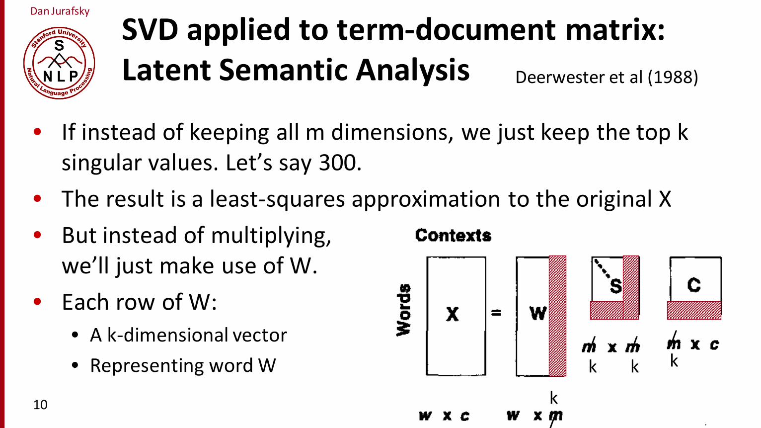
• If instead of keeping all m dimensions, we just keep the top k singular values. Let’s say 300.
• The result is a least-‐squares approximation to the original X• But instead of multiplying,
we’ll just make use of W.• Each row of W:
• A k-‐dimensional vector• Representing word W
10
238 LANDAUER AND DUMAIS
Appendix
An Introduction to Singular Value Decomposition and an LSA Example
Singu la r Value D e c o m p o s i t i o n ( S V D )
A well-known proof in matrix algebra asserts that any rectangular matrix (X) is equal to the product of three other matrices (W, S, and C) of a particular form (see Berry, 1992, and Golub et al., 1981, for the basic math and computer algorithms of SVD). The first of these (W) has rows corresponding to the rows of the original, but has m columns corresponding to new, specially derived variables such that there is no correlation between any two columns; that is, each is linearly independent of the others, which means that no one can be constructed as a linear combination of others. Such derived variables are often called principal components, basis vectors, factors, or dimensions. The third matrix (C) has columns corresponding to the original columns, but m rows composed of derived singular vectors. The second matrix (S) is a diagonal matrix; that is, it is a square m × m matrix with nonzero entries only along one central diagonal. These are derived constants called singular values. Their role is to relate the scale of the factors in the first two matrices to each other. This relation is shown schematically in Figure A1. To keep the connection to the concrete applications of SVD in the main text clear, we have labeled the rows and columns words (w) and contexts (c) . The figure caption defines SVD more formally.
The fundamental proof of SVD shows that there always exists a decomposition of this form such that matrix mu!tiplication of the three derived matrices reproduces the original matrix exactly so long as there are enough factors, where enough is always less than or equal to the smaller of the number of rows or columns of the original matrix. The number actually needed, referred to as the rank of the matrix, depends on (or expresses) the intrinsic dimensionality of the data contained in the cells of the original matrix. Of critical importance for latent semantic analysis (LSA), if one or more factor is omitted (that is, if one or more singular values in the diagonal matrix along with the corresponding singular vectors of the other two matrices are deleted), the reconstruction is a least-squares best approximation to the original given the remaining dimensions. Thus, for example, after constructing an SVD, one can reduce the number of dimensions systematically by, for example, remov- ing those with the smallest effect on the sum-squared error of the approx- imation simply by deleting those with the smallest singular values.
The actual algorithms used to compute SVDs for large sparse matrices of the sort involved in LSA are rather sophisticated and are not described here. Suffice it to say that cookbook versions of SVD adequate for small (e.g., 100 × 100) matrices are available in several places (e.g., Mathematica, 1991 ), and a free software version (Berry, 1992) suitable
Contexts
3= m x m m x c
w x c w x m
Figure A1. Schematic diagram of the singular value decomposition (SVD) of a rectangular word (w) by context (c) matrix (X). The original matrix is decomposed into three matrices: W and C, which are orthonormal, and S, a diagonal matrix. The m columns of W and the m rows of C ' are linearly independent.
for very large matrices such as the one used here to analyze an encyclope- dia can currently be obtained from the WorldWideWeb (http://www.net- l ib.org/svdpack/index.html). University-affiliated researchers may be able to obtain a research-only license and complete software package for doing LSA by contacting Susan Dumais. A~ With Berry 's software and a high-end Unix work-station with approximately 100 megabytes of RAM, matrices on the order of 50,000 × 50,000 (e.g., 50,000 words and 50,000 contexts) can currently be decomposed into representations in 300 dimensions with about 2 - 4 hr of computation. The computational complexity is O(3Dz) , where z is the number of nonzero elements in the Word (w) × Context (c) matrix and D is the number of dimensions returned. The maximum matrix size one can compute is usually limited by the memory (RAM) requirement, which for the fastest of the methods in the Berry package is (10 + D + q ) N + (4 + q)q , where N = w + c and q = min (N, 600), plus space for the W × C matrix. Thus, whereas the computational difficulty of methods such as this once made modeling and simulation of data equivalent in quantity to human experi- ence unthinkable, it is now quite feasible in many cases.
Note, however, that the simulations of adult psycholinguistic data reported here were still limited to corpora much smaller than the total text to which an educated adult has been exposed.
An LSA Example
Here is a small example that gives the flavor of the analysis and demonstrates what the technique can accomplish. A2 This example uses as text passages the titles of nine technical memoranda, five about human computer interaction (HCI) , and four about mathematical graph theory, topics that are conceptually rather disjoint. The titles are shown below.
cl : Human machine interface for ABC computer applications c2: A survey of user opinion of computer system response time c3: The EPS user interface management system c4: System and human system engineering testing of EPS c5: Relation of user perceived response time to error measurement ml : The generation of random, binary, ordered trees m2: The intersection graph of paths in trees m3: Graph minors IV: Widths of trees and well-quasi-ordering m4: Graph minors: A survey
The matrix formed to represent this text is shown in Figure A2. (We discuss the highlighted parts of the tables in due course.) The initial matrix has nine columns, one for each title, and we have given it 12 rows, each corresponding to a content word that occurs in at least two contexts. These are the words in italics. In LSA analyses of text, includ- ing some of those reported above, words that appear in only one context are often omitted in doing the SVD. These contribute little to derivation of the space, their vectors can be constructed after the SVD with little loss as a weighted average of words in the sample in which they oc- curred, and their omission sometimes greatly reduces the computation. See Deerwester, Dumais, Furnas, Landauer, and Harshman (1990) and Dumais (1994) for more on such details. For simplicity of presentation,
A~ Inquiries about LSA computer programs should be addressed to Susan T. Dumais, Bellcore, 600 South Street, Morristown, New Jersey 07960. Electronic mail may be sent via Intemet to [email protected].
A2 This example has been used in several previous publications (e.g., Deerwester et al., 1990; Landauer & Dumais, 1996).
k/
/k
/k
/k
Deerwester et al (1988)
Dan Jurafsky
LSA more details
• 300 dimensions are commonly used• The cells are commonly weighted by a product of two weights
• Local weight: Log term frequency• Global weight: either idf or an entropy measure
11

Dan Jurafsky
Let’s return to PPMI word-‐word matrices
• Can we apply to SVD to them?
12

Dan Jurafsky
SVD applied to term-‐term matrix
19.3 • DENSE VECTORS AND SVD 13
Singular Value Decomposition (SVD) is a method for finding the most impor-tant dimensions of a data set, those dimensions along which the data varies the most.It can be applied to any rectangular matrix and in language processing it was firstapplied to the task of generating embeddings from term-document matrices by Deer-wester et al. (1988) in a model called Latent Semantic Indexing. In this sectionlet’s look just at its application to a square term-context matrix M with |V | rows (onefor each word) and columns (one for each context word)
SVD factorizes M into the product of three square |V |⇥ |V | matrices W , S, andCT . In W each row still represents a word, but the columns do not; each columnnow represents a dimension in a latent space, such that the |V | column vectors areorthogonal to each other and the columns are ordered by the amount of variancein the original dataset each accounts for. S is a diagonal |V |⇥ |V | matrix, withsingular values along the diagonal, expressing the importance of each dimension.The |V |⇥ |V | matrix CT still represents contexts, but the rows now represent the newlatent dimensions and the |V | row vectors are orthogonal to each other.
By using only the first k dimensions, of W, S, and C instead of all |V | dimen-sions, the product of these 3 matrices becomes a least-squares approximation to theoriginal M. Since the first dimensions encode the most variance, one way to viewthe reconstruction is thus as modeling the most important information in the originaldataset.
SVD applied to co-occurrence matrix X:2
666664X
3
777775
|V |⇥ |V |
=
2
666664W
3
777775
|V |⇥ |V |
2
666664
s1 0 0 . . . 00 s2 0 . . . 00 0 s3 . . . 0...
......
. . ....
0 0 0 . . . sV
3
777775
|V |⇥ |V |
2
666664C
3
777775
|V |⇥ |V |
Taking only the top k dimensions after SVD applied to co-occurrence matrix X:2
666664X
3
777775
|V |⇥ |V |
=
2
666664W
3
777775
|V |⇥ k
2
666664
s1 0 0 . . . 00 s2 0 . . . 00 0 s3 . . . 0...
......
. . ....
0 0 0 . . . sk
3
777775
k⇥ k
hC
i
k⇥ |V |
Figure 19.11 SVD factors a matrix X into a product of three matrices, W, S, and C. Takingthe first k dimensions gives a |V |⇥k matrix Wk that has one k-dimensioned row per word thatcan be used as an embedding.
Using only the top k dimensions (corresponding to the k most important singularvalues), leads to a reduced |V |⇥k matrix Wk, with one k-dimensioned row per word.This row now acts as a dense k-dimensional vector (embedding) representing thatword, substituting for the very high-dimensional rows of the original M.3
3 Note that early systems often instead weighted Wk by the singular values, using the product Wk ·Sk asan embedding instead of just the matrix Wk , but this weighting leads to significantly worse embeddings(Levy et al., 2015).
13 (I’m simplifying here by assuming the matrix has rank |V|)
Dan Jurafsky
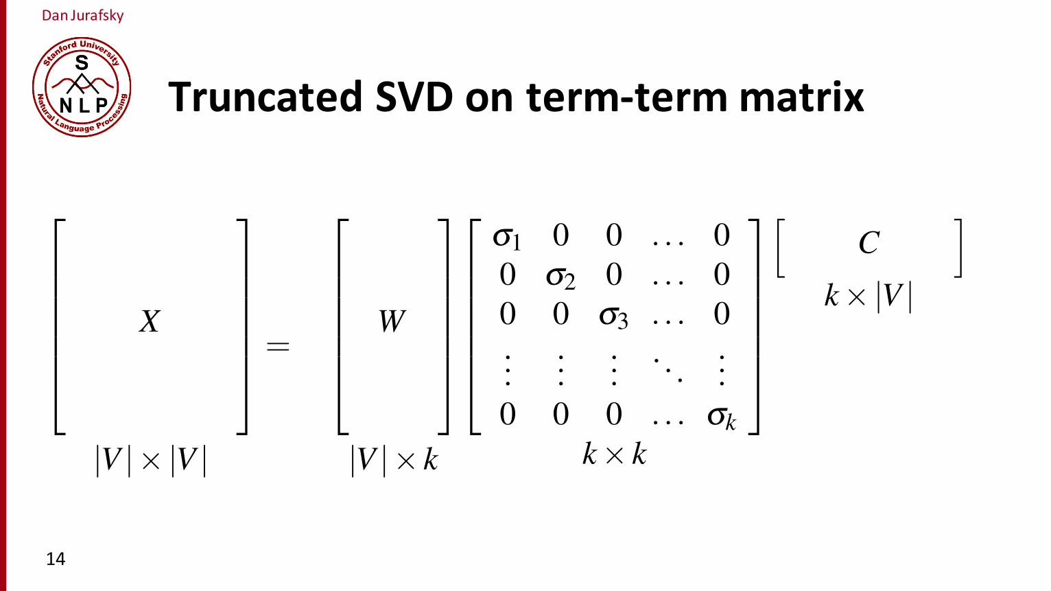
Truncated SVD on term-‐term matrix
19.3 • DENSE VECTORS AND SVD 13
Singular Value Decomposition (SVD) is a method for finding the most impor-tant dimensions of a data set, those dimensions along which the data varies the most.It can be applied to any rectangular matrix and in language processing it was firstapplied to the task of generating embeddings from term-document matrices by Deer-wester et al. (1988) in a model called Latent Semantic Indexing. In this sectionlet’s look just at its application to a square term-context matrix M with |V | rows (onefor each word) and columns (one for each context word)
SVD factorizes M into the product of three square |V |⇥ |V | matrices W , S, andCT . In W each row still represents a word, but the columns do not; each columnnow represents a dimension in a latent space, such that the |V | column vectors areorthogonal to each other and the columns are ordered by the amount of variancein the original dataset each accounts for. S is a diagonal |V |⇥ |V | matrix, withsingular values along the diagonal, expressing the importance of each dimension.The |V |⇥ |V | matrix CT still represents contexts, but the rows now represent the newlatent dimensions and the |V | row vectors are orthogonal to each other.
By using only the first k dimensions, of W, S, and C instead of all |V | dimen-sions, the product of these 3 matrices becomes a least-squares approximation to theoriginal M. Since the first dimensions encode the most variance, one way to viewthe reconstruction is thus as modeling the most important information in the originaldataset.
SVD applied to co-occurrence matrix X:2
666664X
3
777775
|V |⇥ |V |
=
2
666664W
3
777775
|V |⇥ |V |
2
666664
s1 0 0 . . . 00 s2 0 . . . 00 0 s3 . . . 0...
......
. . ....
0 0 0 . . . sV
3
777775
|V |⇥ |V |
2
666664C
3
777775
|V |⇥ |V |
Taking only the top k dimensions after SVD applied to co-occurrence matrix X:2
666664X
3
777775
|V |⇥ |V |
=
2
666664W
3
777775
|V |⇥ k
2
666664
s1 0 0 . . . 00 s2 0 . . . 00 0 s3 . . . 0...
......
. . ....
0 0 0 . . . sk
3
777775
k⇥ k
hC
i
k⇥ |V |
Figure 19.11 SVD factors a matrix X into a product of three matrices, W, S, and C. Takingthe first k dimensions gives a |V |⇥k matrix Wk that has one k-dimensioned row per word thatcan be used as an embedding.
Using only the top k dimensions (corresponding to the k most important singularvalues), leads to a reduced |V |⇥k matrix Wk, with one k-dimensioned row per word.This row now acts as a dense k-dimensional vector (embedding) representing thatword, substituting for the very high-dimensional rows of the original M.3
3 Note that early systems often instead weighted Wk by the singular values, using the product Wk ·Sk asan embedding instead of just the matrix Wk , but this weighting leads to significantly worse embeddings(Levy et al., 2015).
14
Dan Jurafsky
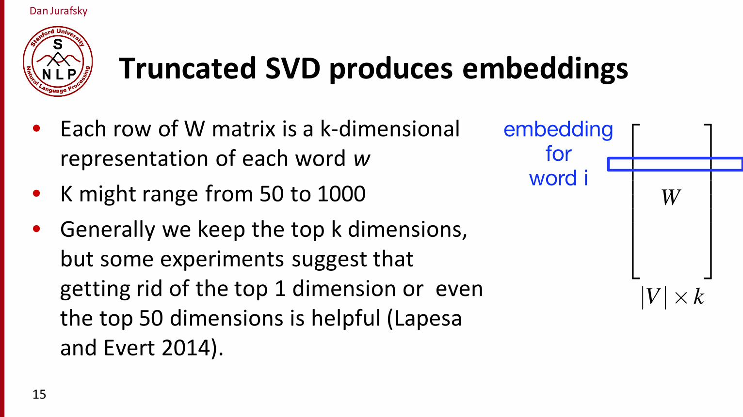
Truncated SVD produces embeddings
15
• Each row of W matrix is a k-‐dimensional representation of each word w
• K might range from 50 to 1000• Generally we keep the top k dimensions,
but some experiments suggest that getting rid of the top 1 dimension or even the top 50 dimensions is helpful (Lapesaand Evert 2014).
19.3 • DENSE VECTORS AND SVD 13
Singular Value Decomposition (SVD) is a method for finding the most impor-tant dimensions of a data set, those dimensions along which the data varies the most.It can be applied to any rectangular matrix and in language processing it was firstapplied to the task of generating embeddings from term-document matrices by Deer-wester et al. (1988) in a model called Latent Semantic Indexing. In this sectionlet’s look just at its application to a square term-context matrix M with |V | rows (onefor each word) and columns (one for each context word)
SVD factorizes M into the product of three square |V |⇥ |V | matrices W , S, andCT . In W each row still represents a word, but the columns do not; each columnnow represents a dimension in a latent space, such that the |V | column vectors areorthogonal to each other and the columns are ordered by the amount of variancein the original dataset each accounts for. S is a diagonal |V |⇥ |V | matrix, withsingular values along the diagonal, expressing the importance of each dimension.The |V |⇥ |V | matrix CT still represents contexts, but the rows now represent the newlatent dimensions and the |V | row vectors are orthogonal to each other.
By using only the first k dimensions, of W, S, and C instead of all |V | dimen-sions, the product of these 3 matrices becomes a least-squares approximation to theoriginal M. Since the first dimensions encode the most variance, one way to viewthe reconstruction is thus as modeling the most important information in the originaldataset.
SVD applied to co-occurrence matrix X:2
666664X
3
777775
|V |⇥ |V |
=
2
666664W
3
777775
|V |⇥ |V |
2
666664
s1 0 0 . . . 00 s2 0 . . . 00 0 s3 . . . 0...
......
. . ....
0 0 0 . . . sV
3
777775
|V |⇥ |V |
2
666664C
3
777775
|V |⇥ |V |
Taking only the top k dimensions after SVD applied to co-occurrence matrix X:2
666664X
3
777775
|V |⇥ |V |
=
2
666664W
3
777775
|V |⇥ k
2
666664
s1 0 0 . . . 00 s2 0 . . . 00 0 s3 . . . 0...
......
. . ....
0 0 0 . . . sk
3
777775
k⇥ k
hC
i
k⇥ |V |
Figure 19.11 SVD factors a matrix X into a product of three matrices, W, S, and C. Takingthe first k dimensions gives a |V |⇥k matrix Wk that has one k-dimensioned row per word thatcan be used as an embedding.
Using only the top k dimensions (corresponding to the k most important singularvalues), leads to a reduced |V |⇥k matrix Wk, with one k-dimensioned row per word.This row now acts as a dense k-dimensional vector (embedding) representing thatword, substituting for the very high-dimensional rows of the original M.3
3 Note that early systems often instead weighted Wk by the singular values, using the product Wk ·Sk asan embedding instead of just the matrix Wk , but this weighting leads to significantly worse embeddings(Levy et al., 2015).
embeddingfor
word i

Dan Jurafsky
Embeddings versus sparse vectors
• Dense SVD embeddings sometimes work better than sparse PPMI matrices at tasks like word similarity• Denoising: low-‐order dimensions may represent unimportant information
• Truncation may help the models generalize better to unseen data.• Having a smaller number of dimensions may make it easier for classifiers to properly weight the dimensions for the task.
• Dense models may do better at capturing higher order co-‐occurrence.
16
Vector Semantics
Embeddings inspired by neural language models: skip-‐grams and CBOW
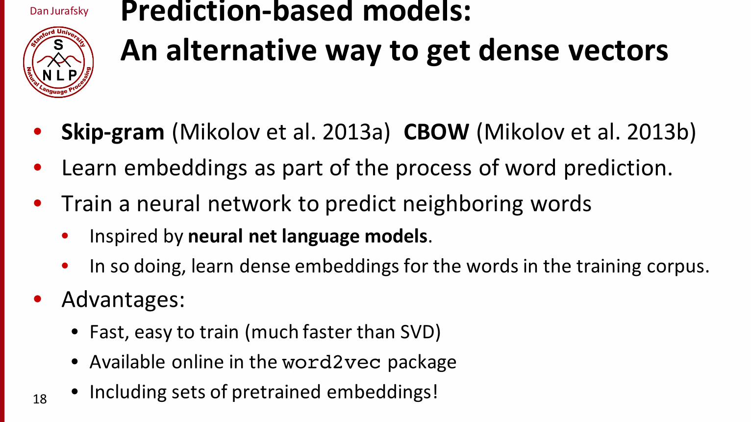
Dan Jurafsky Prediction-‐based models:An alternative way to get dense vectors
• Skip-‐gram (Mikolov et al. 2013a) CBOW (Mikolov et al. 2013b)• Learn embeddings as part of the process of word prediction.• Train a neural network to predict neighboring words• Inspired by neural net language models.• In so doing, learn dense embeddings for the words in the training corpus.
• Advantages:• Fast, easy to train (much faster than SVD)• Available online in the word2vec package• Including sets of pretrained embeddings!18

Dan Jurafsky
Skip-‐grams
• Predict each neighboring word • in a context window of 2C words • from the current word.
• So for C=2, we are given word wt and predicting these 4 words:
19
14 CHAPTER 19 • VECTOR SEMANTICS
This method is sometimes called truncated SVD. SVD is parameterized by k,truncated SVDthe number of dimensions in the representation for each word, typically rangingfrom 500 to 1000. Usually, these are the highest-order dimensions, although forsome tasks, it seems to help to actually throw out a small number of the most high-order dimensions, such as the first 50 (Lapesa and Evert, 2014).
The dense embeddings produced by SVD sometimes perform better than theraw PPMI matrices on semantic tasks like word similarity. Various aspects of thedimensionality reduction seem to be contributing to the increased performance. Iflow-order dimensions represent unimportant information, the truncated SVD may beacting to removing noise. By removing parameters, the truncation may also help themodels generalize better to unseen data. When using vectors in NLP tasks, havinga smaller number of dimensions may make it easier for machine learning classifiersto properly weight the dimensions for the task. And the models may do better atcapturing higher order co-occurrence.
Nonetheless, there is a significant computational cost for the SVD for a large co-occurrence matrix, and performance is not always better than using the full sparsePPMI vectors, so for some applications the sparse vectors are the right approach.Alternatively, the neural embeddings we discuss in the next section provide a popularefficient solution to generating dense embeddings.
19.4 Embeddings from prediction: Skip-gram and CBOW
An alternative to applying dimensionality reduction techniques like SVD to co-occurrence matrices is to apply methods that learn embeddings for words as partof the process of word prediction. Two methods for generating dense embeddings,skip-gram and CBOW (continuous bag of words) (Mikolov et al. 2013, Mikolovskip-gram
CBOW et al. 2013a), draw inspiration from the neural methods for language modeling intro-duced in Chapter 5. Like the neural language models, these models train a networkto predict neighboring words, and while doing so learn dense embeddings for thewords in the training corpus. The advantage of these methods is that they are fast,efficient to train, and easily available online in the word2vec package; code andpretrained embeddings are both available.
We’ll begin with the skip-gram model. The skip-gram model predicts eachneighboring word in a context window of 2C words from the current word. Sofor a context window C = 2 the context is [wt�2,wt�1,wt+1,wt+2] and we are pre-dicting each of these from word wt . Fig. 17.12 sketches the architecture for a samplecontext C = 1.
The skip-gram model actually learns two d-dimensional embeddings for eachword w: the input embedding v and the output embedding v0. These embeddingsinput
embeddingoutput
embedding are encoded in two matrices, the input matrix W and the output matrix W 0. Eachcolumn i of the input matrix W is the 1⇥ d vector embedding vi for word i in thevocabulary. Each row i of the output matrix W 0 is a d ⇥ 1 vector embedding v0i forword i in the vocabulary
Let’s consider the prediction task. We are walking through a corpus of length Tand currently pointing at the tth word w(t), whose index in the vocabulary is j, sowe’ll call it w j (1 < j < |V |). Let’s consider predicting one of the 2C context words,for example w(t+1), whose index in the vocabulary is k (1 < k < |V |). Hence our taskis to compute P(wk|w j).

Dan Jurafsky
Skip-‐grams learn 2 embeddingsfor each w
input embedding v, in the input matrix W• Column i of the input matrix W is the 1×d
embedding vi for word i in the vocabulary.
output embedding vʹ′, in output matrix W’• Row i of the output matrix Wʹ′ is a d × 1
vector embedding vʹ′i for word i in the vocabulary.
20 |V| x d
W’
12
|V|
i
1 2 d…
.
.
.
.
.
.
.
.
d x |V|
W
12
|V|i1 2
d
.
.
.
.
…

Dan Jurafsky
Setup
• Walking through corpus pointing at word w(t), whose index in the vocabulary is j, so we’ll call it wj (1 < j < |V |).
• Let’s predict w(t+1) , whose index in the vocabulary is k (1 < k < |V |). Hence our task is to compute P(wk|wj).
21
Dan Jurafsky
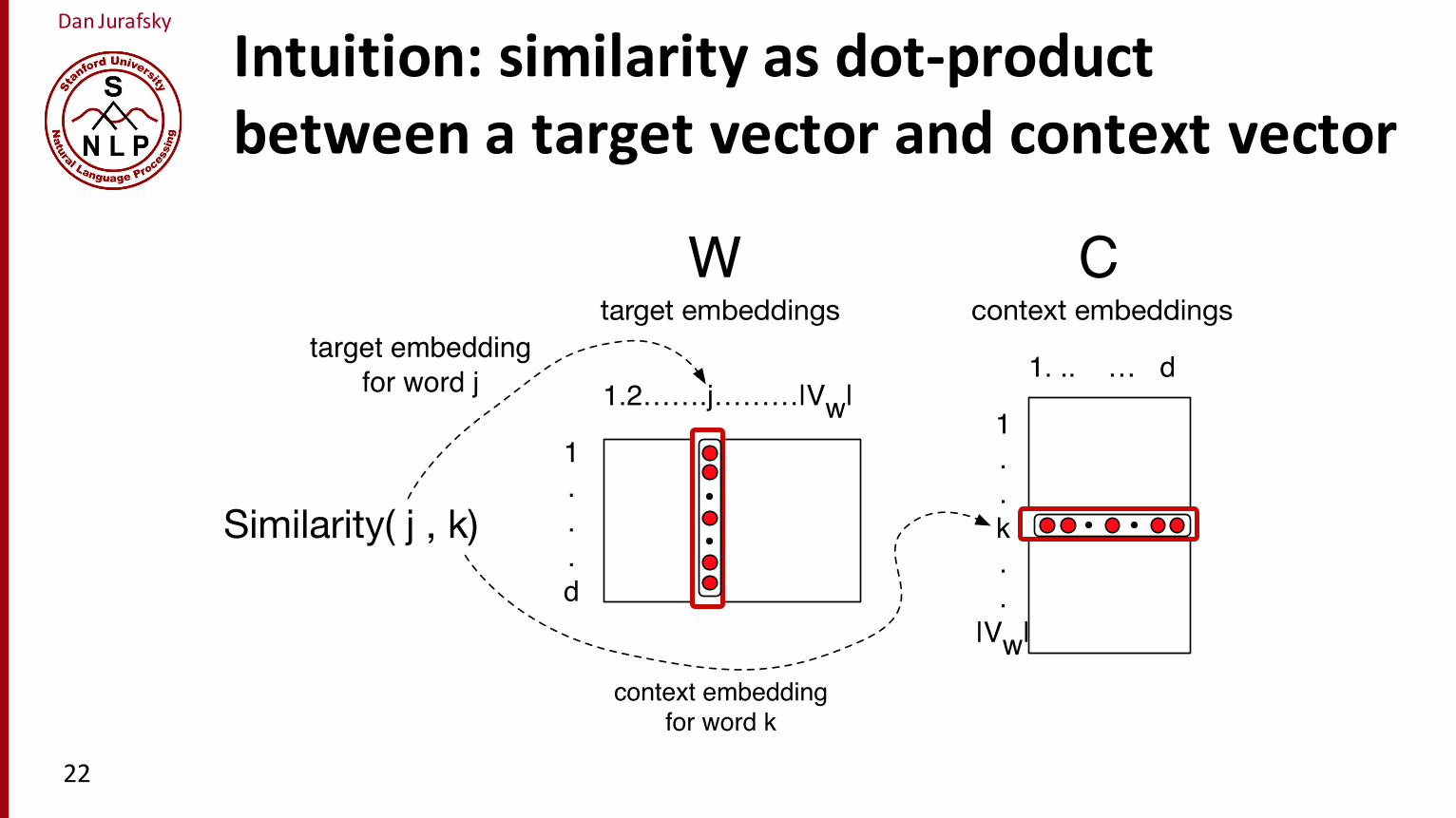
Intuition: similarity as dot-‐productbetween a target vector and context vector
1..k..
|Vw|
1.2…….j………|Vw|
1...d
W
context embeddingfor word k
C1. .. … d
target embeddings context embeddings
Similarity( j , k)
target embeddingfor word j
22
Dan Jurafsky
Similarity is computed from dot product
• Remember: two vectors are similar if they have a high dot product• Cosine is just a normalized dot product
• So:• Similarity(j,k) ∝ ck ·∙ vj
• We’ll need to normalize to get a probability
23

Dan Jurafsky
Turning dot products into probabilities
• Similarity(j,k) = ck · vj
• We use softmax to turn into probabilities
24
6 CHAPTER 16 • SEMANTICS WITH DENSE VECTORS
context words, for example w(t+1), whose index in the vocabulary is k (1 < k < |V |).Hence our task is to compute P(wk|w j).
The heart of the skip-gram computation of the probability p(wk|w j) is computingthe dot product between the vectors for wk and w j, the context vector for wk and thetarget vector for w j. We’ll represent this dot product as ck ·v j, where ck is the contextvector of word k and v j is the target vector for word j. As we saw in the previouschapter, the higher the dot product between two vectors, the more similar they are.(That was the intuition of using the cosine as a similarity metric, since cosine is justa normalized dot product). Fig. 16.4 shows the intuition that the similarity functionrequires selecting out a target vector v j from W , and a context vector ck from C.
1..k..
|Vw|
1.2…….j………|Vw|
1...d
W
context embeddingfor word k
C1. .. … d
target embeddings context embeddings
Similarity( j , k)
target embeddingfor word j
Figure 16.4
Of course, the dot product ck · v j is not a probability, it’s just a number rangingfrom �• to •. We can use the softmax function from Chapter 7 to normalize the dotproduct into probabilities. Computing this denominator requires computing the dotproduct between each other word w in the vocabulary with the target word wi:
p(wk|w j) =exp(ck · v j)P
i2|V | exp(ci · v j)(16.1)
In summary, the skip-gram computes the probability p(wk|w j) by taking the dotproduct between the word vector for j (v j) and the context vector for k (ck), andturning this dot product v j · ck into a probability by passing it through a softmaxfunction.
This version of the algorithm, however, has a problem: the time it takes to com-pute the denominator. For each word wt , the denominator requires computing thedot product with all other words. As we’ll see in the next section, we generally solvethis by using an approximation of the denominator.
CBOW The CBOW (continuous bag of words) model is roughly the mirror im-age of the skip-gram model. Like skip-grams, it is based on a predictive model,but this time predicting the current word wt from the context window of 2L wordsaround it, e.g. for L = 2 the context is [wt�2,wt�1,wt+1,wt+2]
While CBOW and skip-gram are similar algorithms and produce similar embed-dings, they do have slightly different behavior, and often one of them will turn outto be the better choice for any particular task.
16.2.1 Learning the word and context embeddingsWe already mentioned the intuition for learning the word embedding matrix W andthe context embedding matrix C: iteratively make the embeddings for a word more

Dan Jurafsky
Embeddings from W and W’
• Since we have two embeddings, vj and cj for each word wj• We can either:
• Just use vj• Sum them• Concatenate them to make a double-‐length embedding
25
Dan Jurafsky
Learning
• Start with some initial embeddings (e.g., random)• iteratively make the embeddings for a word
• more like the embeddings of its neighbors • less like the embeddings of other words.
26

Dan Jurafsky
Visualizing W and C as a network for doing error backprop
Input layer Projection layer Output layer
wt wt+1
1-hot input vector
1⨉d1⨉|V|
embedding for wtprobabilities ofcontext words
C d ⨉ |V|
x1x2
xj
x|V|
y1y2
yk
y|V|
W|V|⨉d
1⨉|V|27

Dan Jurafsky
One-‐hot vectors
• A vector of length |V| • 1 for the target word and 0 for other words• So if “popsicle” is vocabulary word 5• The one-‐hot vector is• [0,0,0,0,1,0,0,0,0…….0]
28
0 0 0 0 0 … 0 0 0 0 1 0 0 0 0 0 … 0 0 0 0
w0 wj w|V|w1
Dan Jurafsky
29
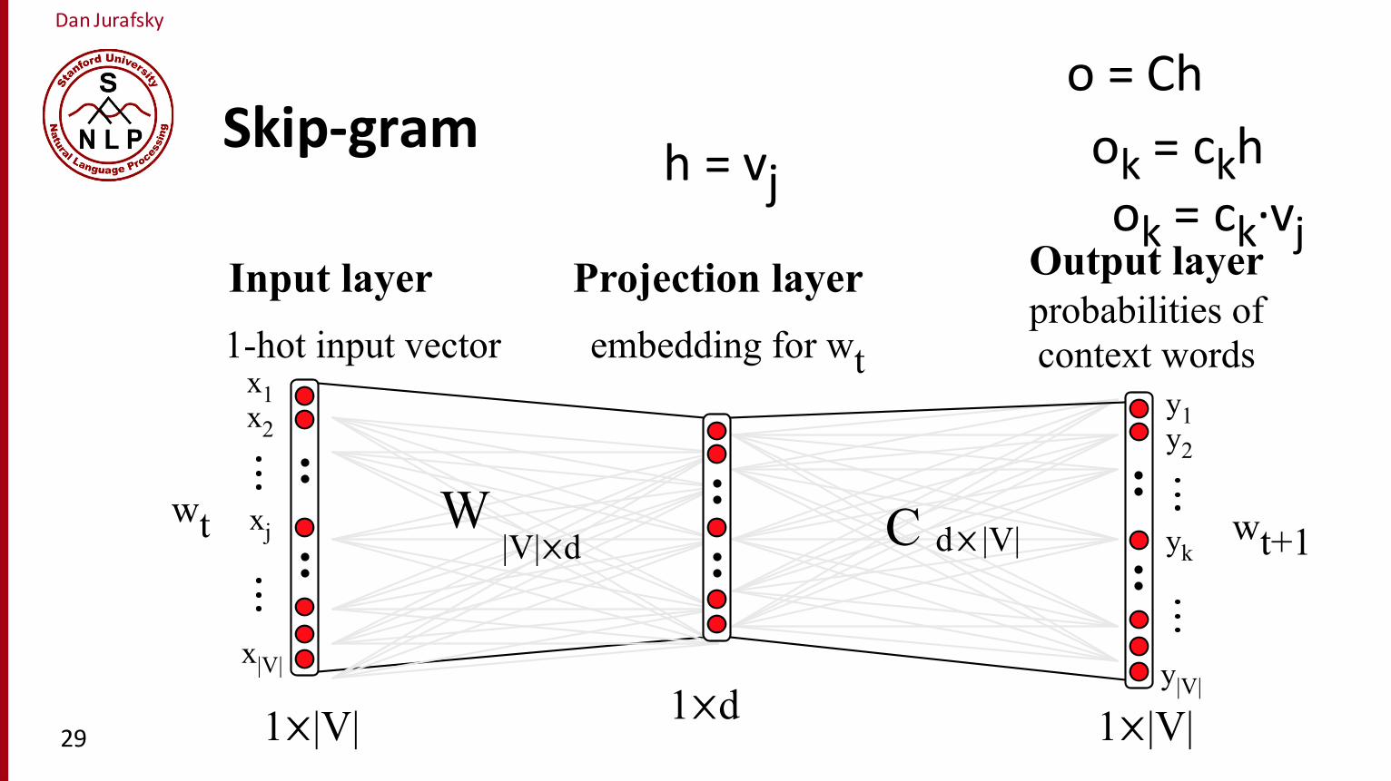
Skip-‐gram h = vj
o = Ch
Input layer Projection layer Output layer
wt wt+1
1-hot input vector
1⨉d1⨉|V|
embedding for wtprobabilities ofcontext words
C d ⨉ |V|
x1x2
xj
x|V|
y1y2
yk
y|V|
W|V|⨉d
1⨉|V|
ok = ckhok = ck·∙vj
Dan Jurafsky
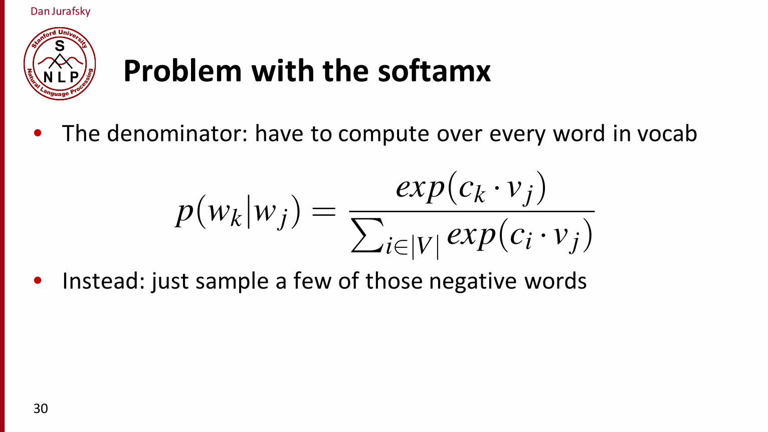
Problem with the softamx
• The denominator: have to compute over every word in vocab
• Instead: just sample a few of those negative words
30
6 CHAPTER 16 • SEMANTICS WITH DENSE VECTORS
context words, for example w(t+1), whose index in the vocabulary is k (1 < k < |V |).Hence our task is to compute P(wk|w j).
The heart of the skip-gram computation of the probability p(wk|w j) is computingthe dot product between the vectors for wk and w j, the context vector for wk and thetarget vector for w j. We’ll represent this dot product as ck ·v j, where ck is the contextvector of word k and v j is the target vector for word j. As we saw in the previouschapter, the higher the dot product between two vectors, the more similar they are.(That was the intuition of using the cosine as a similarity metric, since cosine is justa normalized dot product). Fig. 16.4 shows the intuition that the similarity functionrequires selecting out a target vector v j from W , and a context vector ck from C.
1..k..
|Vw|
1.2…….j………|Vw|
1...d
W
context embeddingfor word k
C1. .. … d
target embeddings context embeddings
Similarity( j , k)
target embeddingfor word j
Figure 16.4
Of course, the dot product ck · v j is not a probability, it’s just a number rangingfrom �• to •. We can use the softmax function from Chapter 7 to normalize the dotproduct into probabilities. Computing this denominator requires computing the dotproduct between each other word w in the vocabulary with the target word wi:
p(wk|w j) =exp(ck · v j)P
i2|V | exp(ci · v j)(16.1)
In summary, the skip-gram computes the probability p(wk|w j) by taking the dotproduct between the word vector for j (v j) and the context vector for k (ck), andturning this dot product v j · ck into a probability by passing it through a softmaxfunction.
This version of the algorithm, however, has a problem: the time it takes to com-pute the denominator. For each word wt , the denominator requires computing thedot product with all other words. As we’ll see in the next section, we generally solvethis by using an approximation of the denominator.
CBOW The CBOW (continuous bag of words) model is roughly the mirror im-age of the skip-gram model. Like skip-grams, it is based on a predictive model,but this time predicting the current word wt from the context window of 2L wordsaround it, e.g. for L = 2 the context is [wt�2,wt�1,wt+1,wt+2]
While CBOW and skip-gram are similar algorithms and produce similar embed-dings, they do have slightly different behavior, and often one of them will turn outto be the better choice for any particular task.
16.2.1 Learning the word and context embeddingsWe already mentioned the intuition for learning the word embedding matrix W andthe context embedding matrix C: iteratively make the embeddings for a word more
Dan Jurafsky
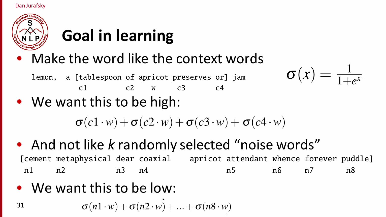
Goal in learning• Make the word like the context words
• We want this to be high:
• And not like k randomly selected “noise words”
• We want this to be low:31
16.2 • EMBEDDINGS FROM PREDICTION: SKIP-GRAM AND CBOW 7
like the embeddings of its neighbors and less like the embeddings of other words.In the version of the prediction algorithm suggested in the previous section, the
probability of a word is computed by normalizing the dot-product between a wordand each context word by the dot products for all words. This probability is opti-mized when a word’s vector is closest to the words that occur near it (the numerator),and further from every other word (the denominator). Such a version of the algo-rithm is very expensive; we need to compute a whole lot of dot products to make thedenominator.
Instead, the most commonly used version of skip-gram, skip-gram with negativesampling, approximates this full denominator.
This section offers a brief sketch of how this works. In the training phase, thealgorithm walks through the corpus, at each target word choosing the surroundingcontext words as positive examples, and for each positive example also choosing knoise samples or negative samples: non-neighbor words. The goal will be to movenegative
samplesthe embeddings toward the neighbor words and away from the noise words.
For example, in walking through the example text below we come to the wordapricot, and let L = 2 so we have 4 context words c1 through c4:
lemon, a [tablespoon of apricot preserves or] jam
c1 c2 w c3 c4
The goal is to learn an embedding whose dot product with each context wordis high. In practice skip-gram uses a sigmoid function s of the dot product, wheres(x) = 1
1+ex . So for the above example we want s(c1 ·w)+s(c2 ·w)+s(c3 ·w)+s(c4 ·w) to be high.
In addition, for each context word the algorithm chooses k noise words accordingto their unigram frequency. If we let k = 2, for each target/context pair, we’ll have 2noise words for each of the 4 context words:
[cement metaphysical dear coaxial apricot attendant whence forever puddle]
n1 n2 n3 n4 n5 n6 n7 n8
We’d like these noise words n to have a low dot-product with our target embed-ding w; in other words we want s(n1 ·w)+s(n2 ·w)+ ...+s(n8 ·w) to be low.
More formally, the learning objective for one word/context pair (w,c) is
logs(c ·w)+kX
i=1
Ewi⇠p(w) [logs(�wi ·w)] (16.2)
That is, we want to maximize the dot product of the word with the actual contextword, and minimize the dot products of the word with the k negative sampled non-neighbor words. The noise words wi are sampled from the vocabulary V accordingto their weighted unigram probability; in practice rather than p(w) it is common touse the weighting p
34 (w).
The learning algorithm starts with randomly initialized W and C matrices, andthen walks through the training corpus moving W and C so as to maximize the objec-tive in Eq. 16.2. An algorithm like stochastic gradient descent is used to iterativelyshift each value so as to maximize the objective, using error backpropagation topropagate the gradient back through the network as described in Chapter 5 (Mikolovet al., 2013a).
In summary, the learning objective in Eq. 16.2 is not the same as the p(wk|w j)defined in Eq. 16.3. Nonetheless, although negative sampling is a different objectivethan the probability objective, and so the resulting dot products will not produce
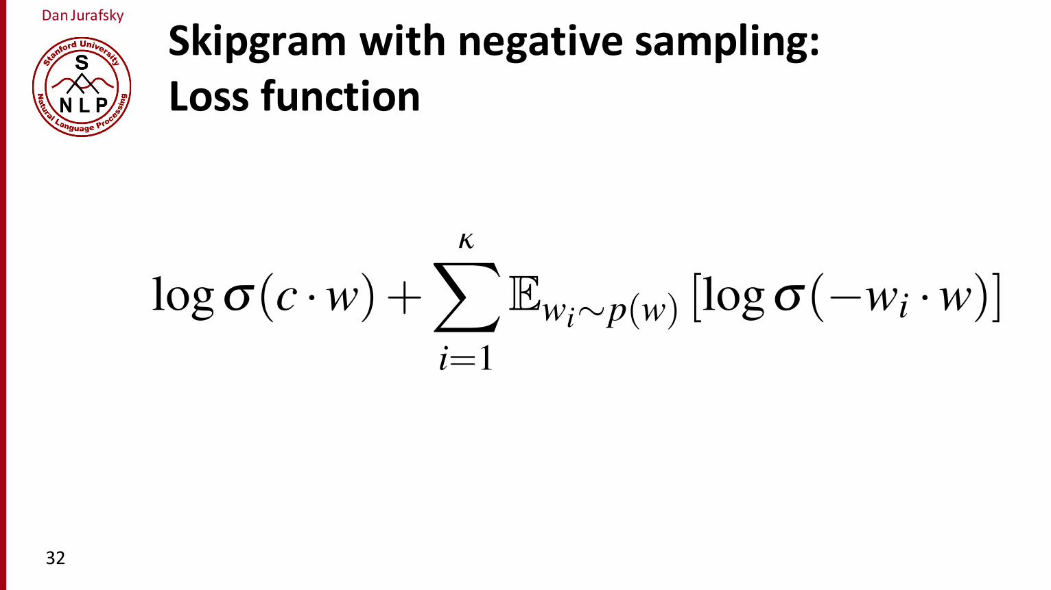
Dan Jurafsky
Skipgram with negative sampling:Loss function
16.2 • EMBEDDINGS FROM PREDICTION: SKIP-GRAM AND CBOW 7
like the embeddings of its neighbors and less like the embeddings of other words.In the version of the prediction algorithm suggested in the previous section, the
probability of a word is computed by normalizing the dot-product between a wordand each context word by the dot products for all words. This probability is opti-mized when a word’s vector is closest to the words that occur near it (the numerator),and further from every other word (the denominator). Such a version of the algo-rithm is very expensive; we need to compute a whole lot of dot products to make thedenominator.
Instead, the most commonly used version of skip-gram, skip-gram with negativesampling, approximates this full denominator.
This section offers a brief sketch of how this works. In the training phase, thealgorithm walks through the corpus, at each target word choosing the surroundingcontext words as positive examples, and for each positive example also choosing knoise samples or negative samples: non-neighbor words. The goal will be to movenegative
samplesthe embeddings toward the neighbor words and away from the noise words.
For example, in walking through the example text below we come to the wordapricot, and let L = 2 so we have 4 context words c1 through c4:
lemon, a [tablespoon of apricot preserves or] jam
c1 c2 w c3 c4
The goal is to learn an embedding whose dot product with each context wordis high. In practice skip-gram uses a sigmoid function s of the dot product, wheres(x) = 1
1+ex . So for the above example we want s(c1 ·w)+s(c2 ·w)+s(c3 ·w)+s(c4 ·w) to be high.
In addition, for each context word the algorithm chooses k noise words accordingto their unigram frequency. If we let k = 2, for each target/context pair, we’ll have 2noise words for each of the 4 context words:
[cement metaphysical dear coaxial apricot attendant whence forever puddle]
n1 n2 n3 n4 n5 n6 n7 n8
We’d like these noise words n to have a low dot-product with our target embed-ding w; in other words we want s(n1 ·w)+s(n2 ·w)+ ...+s(n8 ·w) to be low.
More formally, the learning objective for one word/context pair (w,c) is
logs(c ·w)+kX
i=1
Ewi⇠p(w) [logs(�wi ·w)] (16.2)
That is, we want to maximize the dot product of the word with the actual contextword, and minimize the dot products of the word with the k negative sampled non-neighbor words. The noise words wi are sampled from the vocabulary V accordingto their weighted unigram probability; in practice rather than p(w) it is common touse the weighting p
34 (w).
The learning algorithm starts with randomly initialized W and C matrices, andthen walks through the training corpus moving W and C so as to maximize the objec-tive in Eq. 16.2. An algorithm like stochastic gradient descent is used to iterativelyshift each value so as to maximize the objective, using error backpropagation topropagate the gradient back through the network as described in Chapter 5 (Mikolovet al., 2013a).
In summary, the learning objective in Eq. 16.2 is not the same as the p(wk|w j)defined in Eq. 16.3. Nonetheless, although negative sampling is a different objectivethan the probability objective, and so the resulting dot products will not produce
32

Dan Jurafsky
Relation between skipgrams and PMI!
• If we multiply WW’T
• We get a |V|x|V| matrix M , each entry mij corresponding to some association between input word i and output word j
• Levy and Goldberg (2014b) show that skip-‐gram reaches its optimum just when this matrix is a shifted version of PMI:
WWʹ′T =MPMI −log k • So skip-‐gram is implicitly factoring a shifted version of the PMI
matrix into the two embedding matrices.33
Dan Jurafsky
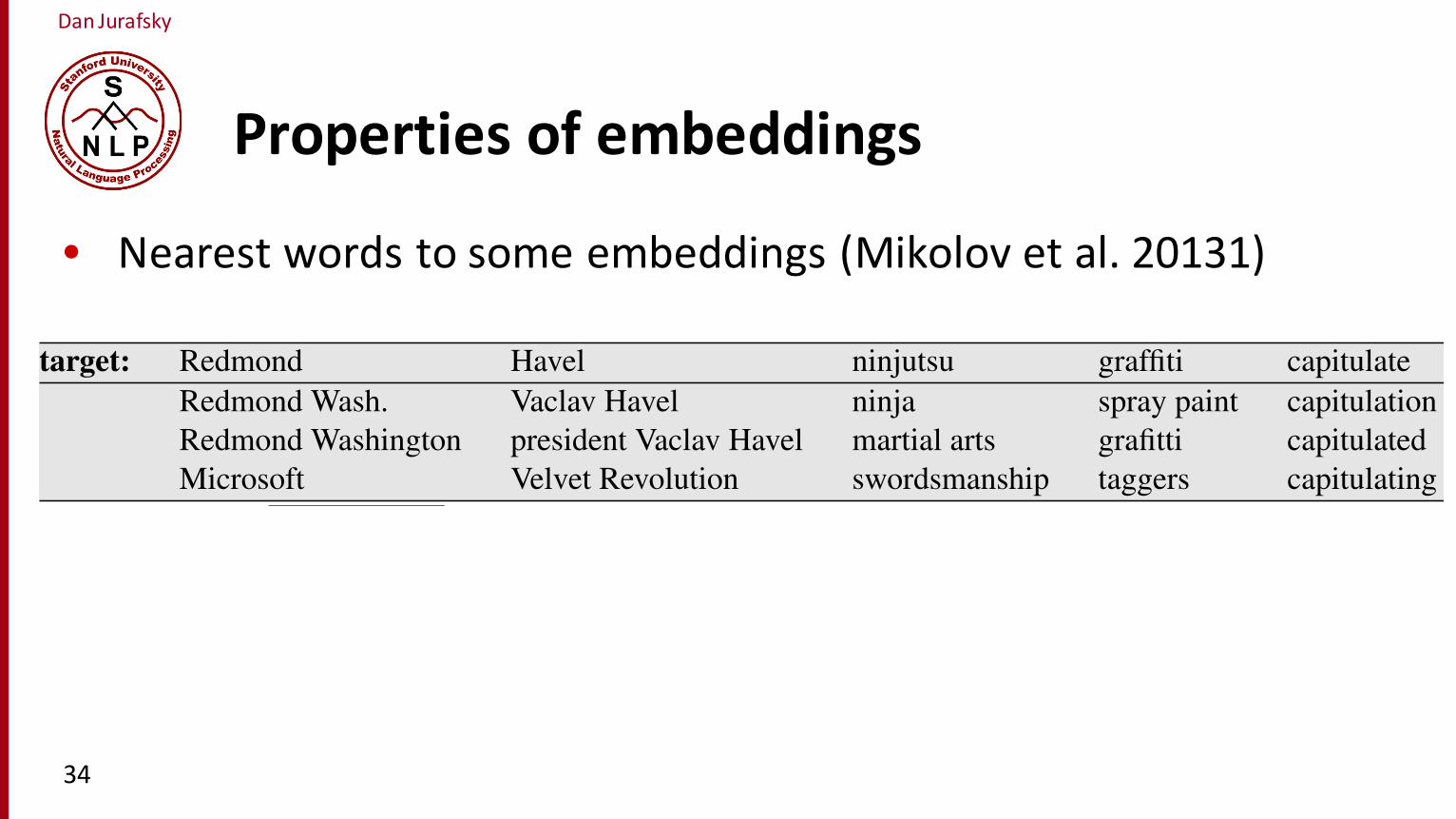
Properties of embeddings
34
• Nearest words to some embeddings (Mikolov et al. 20131)
18 CHAPTER 19 • VECTOR SEMANTICS
matrix is repeated between each one-hot input and the projection layer h. For thecase of C = 1, these two embeddings must be combined into the projection layer,which is done by multiplying each one-hot context vector x by W to give us twoinput vectors (let’s say vi and v j). We then average these vectors
h = W · 12C
X
�c jc, j 6=0
v( j) (19.31)
As with skip-grams, the the projection vector h is multiplied by the output matrixW 0. The result o = W 0h is a 1⇥ |V | dimensional output vector giving a score foreach of the |V | words. In doing so, the element ok was computed by multiplyingh by the output embedding for word wk: ok = v0kh. Finally we normalize this scorevector, turning the score for each element ok into a probability by using the soft-maxfunction.
19.5 Properties of embeddings
We’ll discuss in Section 17.8 how to evaluate the quality of different embeddings.But it is also sometimes helpful to visualize them. Fig. 17.14 shows the words/phrasesthat are most similar to some sample words using the phrase-based version of theskip-gram algorithm (Mikolov et al., 2013a).
target: Redmond Havel ninjutsu graffiti capitulateRedmond Wash. Vaclav Havel ninja spray paint capitulationRedmond Washington president Vaclav Havel martial arts grafitti capitulatedMicrosoft Velvet Revolution swordsmanship taggers capitulating
Figure 19.14 Examples of the closest tokens to some target words using a phrase-basedextension of the skip-gram algorithm (Mikolov et al., 2013a).
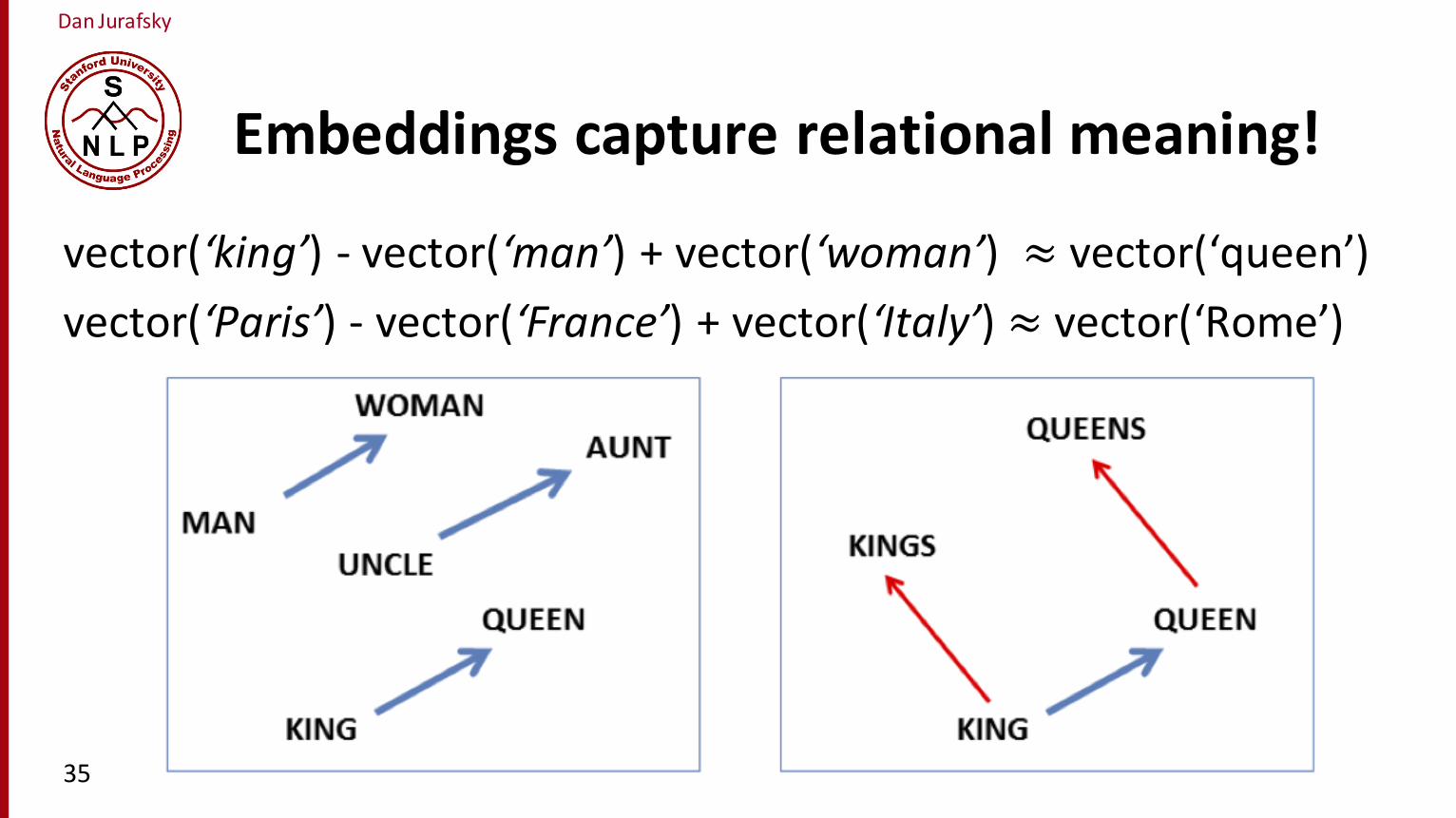
One semantic property of various kinds of embeddings that may play in theirusefulness is their ability to capture relational meanings
Mikolov et al. (2013b) demonstrates that the offsets between vector embeddingscan capture some relations between words, for example that the result of the ex-pression vector(‘king’) - vector(‘man’) + vector(‘woman’) is a vector close to vec-tor(‘queen’); the left panel in Fig. 17.15 visualizes this by projecting a representationdown into 2 dimensions. Similarly, they found that the expression vector(‘Paris’)- vector(‘France’) + vector(‘Italy’) results in a vector that is very close to vec-tor(‘Rome’). Levy and Goldberg (2014a) shows that various other kinds of em-beddings also seem to have this property. We return in the next section to theserelational properties of embeddings and how they relate to meaning compositional-ity: the way the meaning of a phrase is built up out of the meaning of the individualvectors.
19.6 Compositionality in Vector Models of Meaning
To be written.
Dan Jurafsky
Embeddings capture relational meaning!
vector(‘king’) -‐ vector(‘man’) + vector(‘woman’) ≈ vector(‘queen’)vector(‘Paris’) -‐ vector(‘France’) + vector(‘Italy’) ≈ vector(‘Rome’)
35
Vector Semantics
Brown clustering
Dan Jurafsky
Brown clustering
• An agglomerative clustering algorithm that clusters words based on which words precede or follow them
• These word clusters can be turned into a kind of vector• We’ll give a very brief sketch here.
37
Dan Jurafsky
Brown clustering algorithm
• Each word is initially assigned to its own cluster. • We now consider consider merging each pair of clusters. Highest
quality merge is chosen.• Quality = merges two words that have similar probabilities of preceding and following words
• (More technically quality = smallest decrease in the likelihood of the corpus according to a class-‐based language model)
• Clustering proceeds until all words are in one big cluster.
38

Dan Jurafsky
Brown Clusters as vectors
• By tracing the order in which clusters are merged, the model builds a binary tree from bottom to top.
• Each word represented by binary string = path from root to leaf• Each intermediate node is a cluster • Chairman is 0010, “months” = 01, and verbs = 1
39
Brown Algorithm
• Words merged according to contextual similarity
• Clusters are equivalent to bit-string prefixes
• Prefix length determines the granularity of the clustering
011
president
walkrun sprint
chairmanCEO November October
0 100 01
00110010001
10 11000 100 101010

Dan Jurafsky
Brown cluster examples
20 CHAPTER 19 • VECTOR SEMANTICSBrown Algorithm
• Words merged according to contextual similarity
• Clusters are equivalent to bit-string prefixes
• Prefix length determines the granularity of the clustering
011
president
walkrun sprint
chairmanCEO November October
0 100 01
00110010001
10 11000 100 101010
Figure 19.16 Brown clustering as a binary tree. A full binary string represents a word; eachbinary prefix represents a larger class to which the word belongs and can be used as an vectorrepresentation for the word. After Koo et al. (2008).
After clustering, a word can be represented by the binary string that correspondsto its path from the root node; 0 for left, 1 for right, at each choice point in the binarytree. For example in Fig. 19.16, the word chairman is the vector 0010 and Octoberis 011. Since Brown clustering is a hard clustering algorithm (each word has onlyhard clustering
cluster), there is just one string per word.Now we can extract useful features by taking the binary prefixes of this bit string;
each prefix represents a cluster to which the word belongs. For example the string 01in the figure represents the cluster of month names {November, October}, the string0001 the names of common nouns for corporate executives {chairman, president},1 is verbs {run, sprint, walk}, and 0 is nouns. These prefixes can then be usedas a vector representation for the word; the shorter the prefix, the more abstractthe cluster. The length of the vector representation can thus be adjusted to fit theneeds of the particular task. Koo et al. (2008) improving parsing by using multiplefeatures: a 4-6 bit prefix to capture part of speech information and a full bit string torepresent words. Spitkovsky et al. (2011) shows that vectors made of the first 8 or9-bits of a Brown clustering perform well at grammar induction. Because they arebased on immediately neighboring words, Brown clusters are most commonly usedfor representing the syntactic properties of words, and hence are commonly used asa feature in parsers. Nonetheless, the clusters do represent some semantic propertiesas well. Fig. 19.17 shows some examples from a large clustering from Brown et al.(1992).
Friday Monday Thursday Wednesday Tuesday Saturday Sunday weekends Sundays SaturdaysJune March July April January December October November September Augustpressure temperature permeability density porosity stress velocity viscosity gravity tensionanyone someone anybody somebodyhad hadn’t hath would’ve could’ve should’ve must’ve might’veasking telling wondering instructing informing kidding reminding bothering thanking deposingmother wife father son husband brother daughter sister boss unclegreat big vast sudden mere sheer gigantic lifelong scant colossaldown backwards ashore sideways southward northward overboard aloft downwards adriftFigure 19.17 Some sample Brown clusters from a 260,741-word vocabulary trained on 366million words of running text (Brown et al., 1992). Note the mixed syntactic-semantic natureof the clusters.
Note that the naive version of the Brown clustering algorithm described above isextremely inefficient — O(n5): at each of n iterations, the algorithm considers eachof n2 merges, and for each merge, compute the value of the clustering by summingover n2 terms. because it has to consider every possible pair of merges. In practicewe use more efficient O(n3) algorithms that use tables to pre-compute the values foreach merge (Brown et al. 1992, Liang 2005).
40

Dan Jurafsky
Class-‐based language model
• Suppose each word was in some class ci:
41
19.7 • BROWN CLUSTERING 19
Figure 19.15 Vector offsets showing relational properties of the vector space, shown byprojecting vectors onto two dimensions using PCA. In the left panel, ’king’ - ’man’ + ’woman’is close to ’queen’. In the right, we see the way offsets seem to capture grammatical number.(Mikolov et al., 2013b).
19.7 Brown Clustering
Brown clustering (Brown et al., 1992) is an agglomerative clustering algorithm forBrownclustering
deriving vector representations of words by clustering words based on their associa-tions with the preceding or following words.
The algorithm makes use of the class-based language model (Brown et al.,class-basedlanguage model
1992), a model in which each word w 2V belongs to a class c 2C with a probabilityP(w|c). Class based LMs assigns a probability to a pair of words wi�1 and wi bymodeling the transition between classes rather than between words:
P(wi|wi�1) = P(ci|ci�1)P(wi|ci) (19.32)
The class-based LM can be used to assign a probability to an entire corpus givena particularly clustering C as follows:
P(corpus|C) =nY
i�1
P(ci|ci�1)P(wi|ci) (19.33)
Class-based language models are generally not used as a language model for ap-plications like machine translation or speech recognition because they don’t workas well as standard n-grams or neural language models. But they are an importantcomponent in Brown clustering.
Brown clustering is a hierarchical clustering algorithm. Let’s consider a naive(albeit inefficient) version of the algorithm:
1. Each word is initially assigned to its own cluster.2. We now consider consider merging each pair of clusters. The pair whose
merger results in the smallest decrease in the likelihood of the corpus (accord-ing to the class-based language model) is merged.
3. Clustering proceeds until all words are in one big cluster.
Two words are thus most likely to be clustered if they have similar probabilitiesfor preceding and following words, leading to more coherent clusters. The result isthat words will be merged if they are contextually similar.
By tracing the order in which clusters are merged, the model builds a binary treefrom bottom to top, in which the leaves are the words in the vocabulary, and eachintermediate node in the tree represents the cluster that is formed by merging itschildren. Fig. 19.16 shows a schematic view of a part of a tree.