demand response elasticities analysis - bpa.gov · demand response elasticities analysis . february...
TRANSCRIPT
Demand Response Elasticities Analysis
February 16, 2018
Bonneville Power Administration 905 NE 11th Avenue Portland, OR 97232
Disclaimer on Presented Research Results: Cadmus is the research, development, and evaluation contractor hired by Bonneville Power Administration to provide this body of work. The content is not intended to create, does not create, and may not be relied upon to create any rights, substantive or procedural, enforceable at law by any party in any matter civil or criminal. Opinions or points of view expressed on this report represent a consensus of the authors and do not necessarily represent the official position or policies of Bonneville Power Administration and/or the U.S. Department of Energy. Any products and manufacturers discussed on this site are presented for informational purposes only and do not constitute product approval or endorsement by Bonneville Power Administration and/or the U.S. Department of Energy.

Prepared by: Jim Stewart, Ph.D.
Hossein Haeri, Ph.D. Lakin Garth
The Cadmus Group LLC
Table of Contents i
Table of Contents Acknowledgements ...................................................................................................................................... iii
1 Demand Response Elasticity Analysis ..................................................................................................... 1
1.1 Executive Summary ....................................................................................................................... 1
1.2 Methodology ................................................................................................................................. 2
1.2.1 Data Sources ......................................................................................................................... 3
1.3 Model ............................................................................................................................................ 5
1.4 Estimation ..................................................................................................................................... 6
1.4.1 Demand Response Supply Elasticities for Public Utilities ................................................... 10
1.4.2 Comparison to Demand Response Elasticities for Investor-Owned Utilities ..................... 13
1.4.3 Robustness of Elasticity Estimates ..................................................................................... 14
1.4.4 Impact of Customer Characteristics on Utility Customer Supply of Demand Response Capacity .......................................................................................................................................... 17
1.5 Application of Public Utility Elasticity Estimates to Achievable Potential .................................. 20
1.6 Conclusion ................................................................................................................................... 24
List of Tables Table 1. Summary Statistics for Public Utilities ............................................................................................ 4
Table 2. Demand Response Customer Supply Elasticities for Public Utilities ............................................. 11
Table 3. Demand Response Supply Elasticity Estimates for All Utilities ..................................................... 13
Table 4. Robustness Tests for Estimated Elasticities .................................................................................. 16
Table 5. Demand Response Supply Elasticities as a Function of Customer Characteristics ....................... 19
Table 6. Incentive Payment and Achievable Potential Amounts for Demand Response Products ............ 21
List of Figures Figure 1. Hypothetical EIA Data .................................................................................................................... 6
Figure 2. Demand Response Capacity Market Equilibria .............................................................................. 7
Figure 3. Biased Elasticity Estimates by Ignoring Market Equilibria ............................................................. 8
Figure 4. Unbiased Elasticity Estimates from Instrumental Variables .......................................................... 9
Figure 5. Percentage Impacts of Residential Customer Characteristics on Demand Response Supply Elasticities ................................................................................................................................. 20

Table of Contents ii
Figure 6. Residential DLC Products’ 20-Year Base Case Achievable Potential Estimates, Winter .............. 22
Figure 7. Residential DLC Products’ 20-Year Base Case Achievable Potential Estimates, Summer ............ 22
Figure 8. C&I Demand Curtailment 20-Year Base Case Achievable Potential Estimates, Winter ............... 23
Figure 9. Nonresidential 20-Year Base Case Achievable Potential Estimates, Summer ............................. 24

Acknowledgements iii
Acknowledgements
This work was sponsored by Bonneville Power Administration. Cadmus would like to thank the invaluable support and guidance from BPA project manager Thomas Brim, technical advisor Frank Brown, the BPA contracting officer’s technical representative (COTR) Melanie Smith, BPA’s Distributed Energy Resources Program manager Lee Hall, and BPA program staff including Cara Ford, Gwen Resendes, and Lori Barnett. Without their support, Cadmus could not have completed this project. Cadmus also owes a debt of gratitude to the many Power customers, regional stakeholders, DER service providers, and end-use customers who provided data instrumental to this study. Any remaining errors and omissions are Cadmus’.
Demand Response Elasticity Analysis
1 Demand Response Elasticity Analysis
1.1 Executive Summary Quantity megawatt (MW)-price points on the supply curves, determined through Bonneville Power Administration’s (BPA) Demand Response Potential Study, represent static point estimates, assuming typical or average incentive amounts. The curves do not account for the ability of a demand response program administrator to vary customer incentive payments to increase or decrease the supply of demand response capacity.
Understanding the elasticity of customer-supplied demand response capacity is of significant importance to the BPA, its public power customer utilities, regional stakeholders, and policymakers. Utility demand for peak capacity is likely to grow, and demand response is a viable and often lowest-cost option for meeting this demand. Utilities will be able to acquire more demand response capacity but only to the extent that utility customers are willing to supply.
Moreover, utilities are using demand response capacity for other purposes, including for reserves, high-frequency balancing of system supply and demand, integrating intermittent renewable energy generation resources, and managing distribution bottlenecks to avoid costly upgrades to their local distribution systems.1 Recent advances in distribution system controls and communication technologies have made these new applications of demand response possible and should increase utility demand for demand response. It is therefore important for utilities and policymakers to know the price elasticity of demand response supply.
Cadmus performed an elasticity study to estimate the amount of demand response capacity that could be achieved through changes in customer incentive payments. This study analyzed data from 2010 to 2015 on utility demand response programs from the U.S. Energy Information Administration (EIA) Form 861, which collects comprehensive information about utility demand response programs, including capacity from demand response and customer incentive payments for providing capacity.
For public utilities, which include cooperatives, municipalities, and political subdivisions such as public utility districts, the analysis found that the supply of demand response capacity had a price-inelasticity of less than one, meaning that a 1% increase in customer incentives leads to a less than 1% increase in demand response capacity. The estimates of elasticity of supply capacity equaled 0.302, 0.426, and 0.539 for residential, commercial, and industrial customers of public utilities, respectively.2 For example, the estimated elasticity of supply of demand response capacity in the residential sector implies that a 1 Potter, Jennifer, and Peter Cappers. Demand Response Advanced Controls Framework and Assessment of
Enabling Technology Costs. August 2017. Available online: https://emp.lbl.gov/sites/default/files/demand_response_advanced_controls_framework_and_cost_assessment_final_published.pdf
2 The U.S. Energy Information Administration considers agricultural customers to be “industrial.”
Demand Response Elasticity Analysis
1% increase in customer incentives increases demand response capacity by about 0.3%. The elasticity of supply of demand response capacity from residential and commercial customers was lower for customers of public utilities than of investor-owned utilities (IOUs), which means that public utilities may face higher costs of obtaining peak capacity via demand response from these customer classes. As it relates to BPA’s Demand Response Potential Study, the results from this analysis indicate that potentially significantly higher incentives may be required to move from the level of capacity supplied by demand response in the base case achievable potential to the amounts estimated in the high case scenario.
In the residential sector, differences in supply elasticities can also be explained by customer demographic characteristics such as education, urban residency, and customer energy end uses such as space heating fuel. Utilities serving less educated or rural customers may face higher costs of obtaining peak reductions using demand response.
1.2 Methodology Cadmus based this study’s methodology on a collection of EIA Form 861 data for individual utilities and on panel regression analysis of utility customer supply of demand response capacity as a function of utility incentive payments. Cadmus estimated separate equations for the residential, commercial, and industrial sectors because the willingness of customers to supply peak capacity differs across these sectors.
The panel regression reflects two key elements of the market for demand response capacity in the Pacific Northwest: individual supply decisions of a large number of utility customers and utility efforts to minimize the cost of acquiring capacity from traditional generation and demand response resources. As explained further below, utility capacity payments to customers and customer supply of demand response capacity constitute a market equilibrium between the utility and its customers. Utilities offer incentives to customers for supplying capacity, and customers respond with peak reductions if the incentives are sufficient.
Because the incentives that utilites offer depend on their demand for demand response capacity, the supply of demand response capacity will be endogenous, that is, the equilibrium price and supply of capacity will depend on both customer cost of supply and utility demand for demand response capacity.
To account for this endogeneity, Cadmus estimated the demand response supply elasticities by instrumental variables two-stage least squares (IV-2SLS), using utility capacity costs as an instrumental variable for the utility’s customer incentive payments. Instrumental variables estimation is expected to
Demand Response Elasticity Analysis
produce an unbiased estimate of the supply elasticities, assuming the instrumental variables satisfy the model assumptions.3
1.2.1 Data Sources Cadmus collected data from EIA Form 861 for 2010 through 2015. In 2015, the EIA database contained data for 421 utilities with demand response capacity, including 293 public utilities (e.g., municipal, cooperative, and political subdivision utilities). These public utilities represent a substantial part of the market, accounting for roughly 30% of the national potential demand response capacity and nearly 30% of national peak demand between 2010 and 2015. The Cadmus analysis focused primarily on estimating elasticities for public utilities, although, for comparison, we also estimated elasticities for all utilities (publics and private utilities).
The analysis sample comprises annual observations of MW capacity and customer incentive payments for 208 public utilities from 2010 through 2015. Cadmus limited the analysis sample to utilities offering demand response programs in two or more years, since identification of the demand response supply elasticities should depend on the variation of demand response capacity and incentives within, not between, individual utilities. During this six-year period, customers of these utilities supplied a total of about 6.2 GW (6200 MW) of demand response capacity.
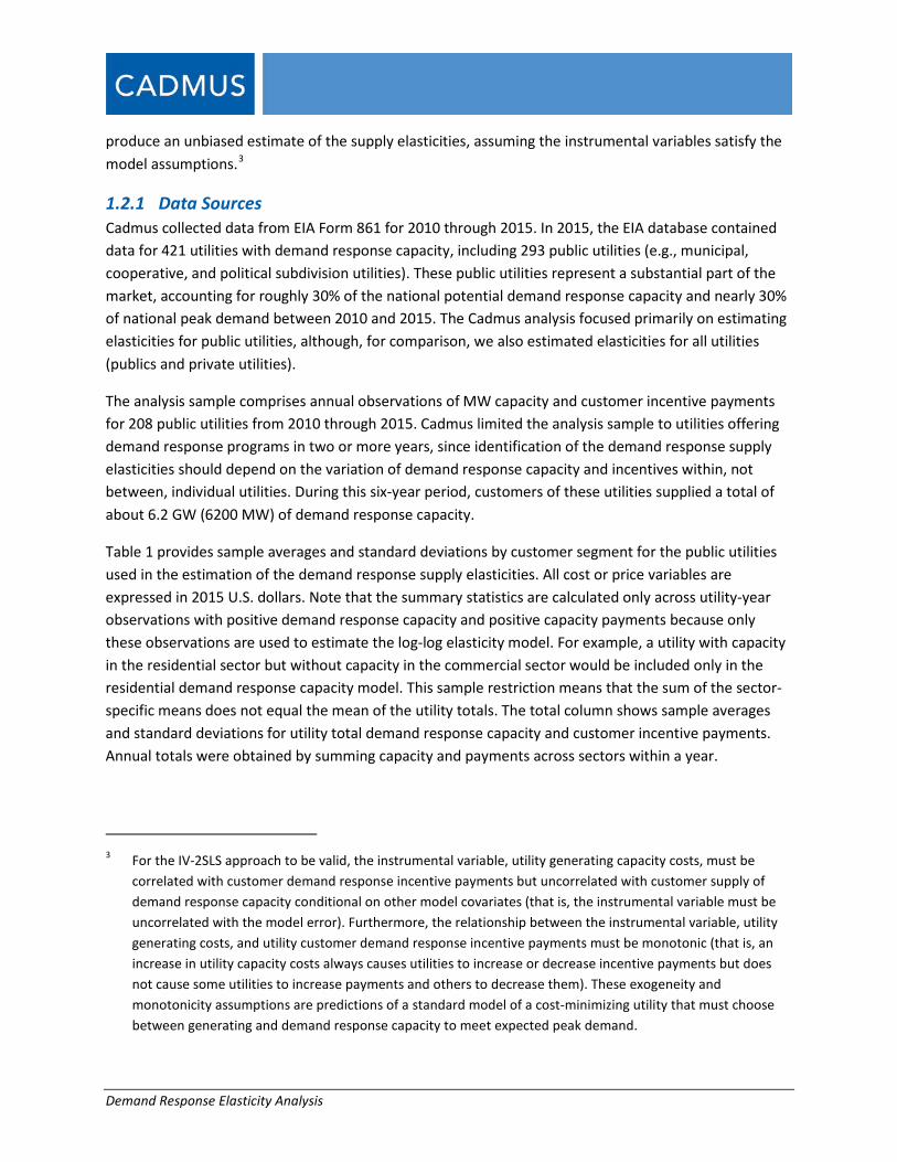
Table 1 provides sample averages and standard deviations by customer segment for the public utilities used in the estimation of the demand response supply elasticities. All cost or price variables are expressed in 2015 U.S. dollars. Note that the summary statistics are calculated only across utility-year observations with positive demand response capacity and positive capacity payments because only these observations are used to estimate the log-log elasticity model. For example, a utility with capacity in the residential sector but without capacity in the commercial sector would be included only in the residential demand response capacity model. This sample restriction means that the sum of the sector-specific means does not equal the mean of the utility totals. The total column shows sample averages and standard deviations for utility total demand response capacity and customer incentive payments. Annual totals were obtained by summing capacity and payments across sectors within a year.
3 For the IV-2SLS approach to be valid, the instrumental variable, utility generating capacity costs, must be
correlated with customer demand response incentive payments but uncorrelated with customer supply of demand response capacity conditional on other model covariates (that is, the instrumental variable must be uncorrelated with the model error). Furthermore, the relationship between the instrumental variable, utility generating costs, and utility customer demand response incentive payments must be monotonic (that is, an increase in utility capacity costs always causes utilities to increase or decrease incentive payments but does not cause some utilities to increase payments and others to decrease them). These exogeneity and monotonicity assumptions are predictions of a standard model of a cost-minimizing utility that must choose between generating and demand response capacity to meet expected peak demand.
Demand Response Elasticity Analysis
Table 1. Summary Statistics for Public Utilities
Residential Commercial Industrial Total
Potential Demand Response Capacity (MW per reporting utility))
16.4 13.8 34.2 29.7 (39.8) (31.2) (98.9) (73.8)
Customer Incentives ($000) per sector per reporting utility
460.5 407.7 1,564.0 884.1 (1,621.4) (1,232.3) (5,502.1) (3,337.5)
ln (Potential Demand Response Capacity [MW])
1.689 1.123 1.993 2.233 (1.423) (1.749) (1.671) (1.462)
ln (Customer Incentives [$000]) 4.238 3.727 4.900 4.643
(1.956) (2.176) (2.215) (2.054)
NERC Region: FRCC (% of total reported) 0.019 0.054 0.026 0.029
(0.138) (0.226) (0.158) (0.169)
NERC Region: MRO 0.464 0.413 0.291 0.390
(0.499) (0.493) (0.455) (0.488)
NERC Region: NPCC 0.024 0.027 0.000 0.021
(0.154) (0.162) 0.000 (0.142)
NERC Region: RFC 0.104 0.070 0.112 0.113
(0.305) (0.256) (0.316) (0.317)
NERC Region: SERC 0.246 0.198 0.250 0.234
(0.431) (0.399) (0.434) (0.424)
NERC Region: SPP 0.039 0.084 0.148 0.080
(0.194) (0.278) (0.356) (0.272)
NERC Region: TRE 0.031 0.050 0.087 0.048
(0.173) (0.219) (0.282) (0.213)
NERC Region: WECC 0.073 0.104 0.087 0.085
(0.260) (0.306) (0.282) (0.279)
Cooperative (% of total reported) 0.679 0.530 0.577 0.663
(0.467) (0.500) (0.495) (0.473)
Municipal 0.293 0.430 0.362 0.294
(0.456) (0.496) (0.482) (0.456)
Political Subdivision 0.028 0.040 0.061 0.044
(0.164) (0.197) (0.240) (0.205) Number of utilities 154 81 60 208 Number of observations 617 298 196 821 Notes: Table reports sample means across utilities and years. Sample standard deviations in parentheses. The NERC region and utility ownership variables are 0-1 indicator variables. ln denotes the natural logarithm. See text for analysis sample selection and variable definitions. On average, public utilities in the sample obtained 16 MW of annual demand response capacity from residential customers, 14 MW from commercial customers, and 34 MW from industrial customers. Annual demand response capacity varied widely within and between utilities, as shown by the sample standard deviations, which were two to three times as large as the sample means. Public utilities paid an average of $0.46 million per year in incentives to residential customers, $0.41 million per year to commercial customers, and $1.6 million per year to industrial customers.
Demand Response Elasticity Analysis
The North American Electric Reliability Corporation (NERC) region variables are binary (0 or 1), indicating the location of the utility in one of eight NERC regions.4 The sample means for the NERC variables show the proportion of utility-year observations from the different regions. Of residential observations, about 46% came from public utility demand response programs operated in the upper Midwest (MRO NERC) region, 10% were in the Middle Atlantic and East North Central (RFC) regions, 25% were in the Southeast (SERC) region, and 7% were in the Mountain or Coastal West (WECC) regions. Sixty-eight percent of public utilities with residential demand response capacity were cooperatives, 29% were municipalities, and 3% were political subdivisions. Utilities with commercial or industrial demand response capacity were more likely to be municipalities. A small number of annual observations had either zero demand response capacity or zero customer incentive payments. Because Cadmus estimated a double-log elasticity model, these observations were not used in the main estimation.
1.3 Model Cadmus estimated the following panel regression of the natural logarithm for supply of demand response capacity in MW (q) from customers of utility j.
Equation 1 qjt =α + βpjt + τjt + εjt
Where:
α = a constant
pjt = the natural logarithm of incentive payments utility j pays customers in year t
τ jt = a time-trend for utility j
ε jt = equals idiosyncratic random error for utility j in period t
As the equation takes a log-log form, the coefficient β can be interpreted as a supply elasticity. The time trend captures utility-specific trends regarding the availability and cost of customer supplies for demand response capacity. For example, increasing central air conditioning penetration in homes would reduce the supply costs for residential customers. Similarly, innovations in two-way communication and control of utility customer appliances—sometimes referred to as the “internet of things”—have reduced the customer costs of supplying demand response capacity. The inclusion of utility-specific time-trends accounts for overall growth in the supply of demand response capacity over the analysis period, but it allows utilities to follow different trends.
4 NERC is responsible for the reliability of bulk power transmission in the United States. It sets standards for
power systems operation and assesses resource adequacy across the country. The continental United States is divided into eight NERC regions: the Florida Reliability Coordinating Council (FRCC), Midwest Reliability Organization (MRO), the Northeast Power Coordinating Council (NPCC), Reliability First (RF), SERC Reliability Council, Southwest Power Pool (SPP), Texas Reliability Entity (TRE), and the Western Electricity Coordinating Council (WECC).
Demand Response Elasticity Analysis
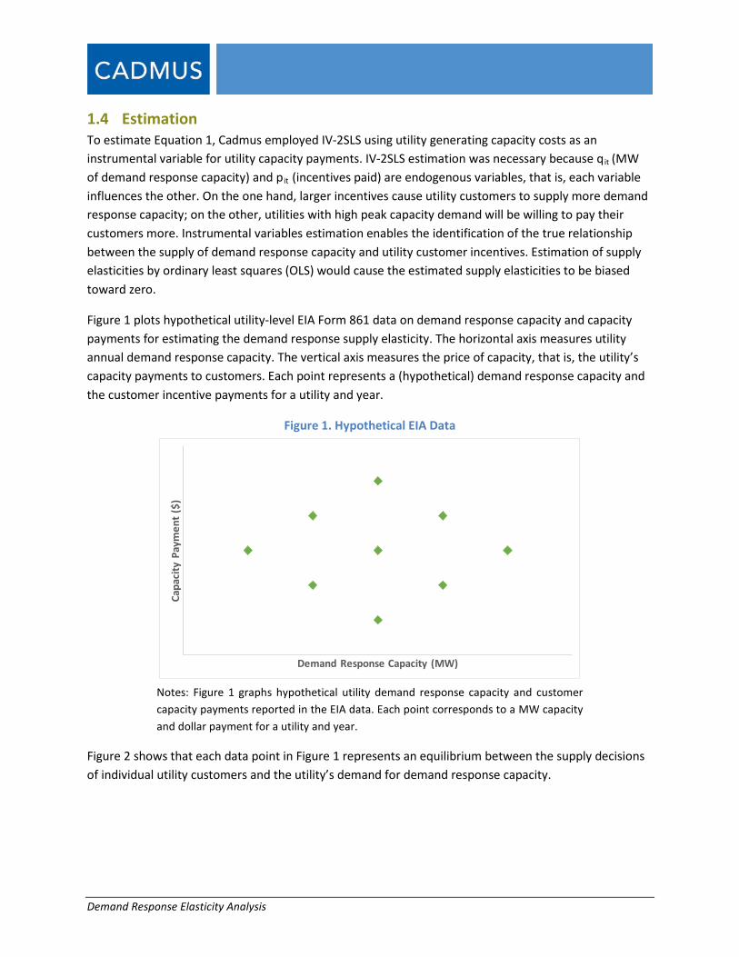
1.4 Estimation To estimate Equation 1, Cadmus employed IV-2SLS using utility generating capacity costs as an instrumental variable for utility capacity payments. IV-2SLS estimation was necessary because qit (MW of demand response capacity) and pit (incentives paid) are endogenous variables, that is, each variable influences the other. On the one hand, larger incentives cause utility customers to supply more demand response capacity; on the other, utilities with high peak capacity demand will be willing to pay their customers more. Instrumental variables estimation enables the identification of the true relationship between the supply of demand response capacity and utility customer incentives. Estimation of supply elasticities by ordinary least squares (OLS) would cause the estimated supply elasticities to be biased toward zero.
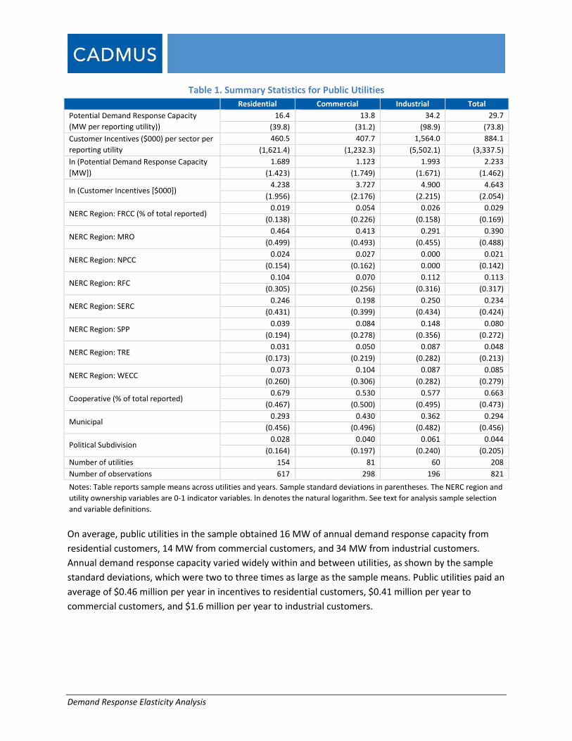
Figure 1 plots hypothetical utility-level EIA Form 861 data on demand response capacity and capacity payments for estimating the demand response supply elasticity. The horizontal axis measures utility annual demand response capacity. The vertical axis measures the price of capacity, that is, the utility’s capacity payments to customers. Each point represents a (hypothetical) demand response capacity and the customer incentive payments for a utility and year.
Figure 1. Hypothetical EIA Data
Capa
city
Pay
men
t ($)
Demand Response Capacity (MW)
Notes: Figure 1 graphs hypothetical utility demand response capacity and customer capacity payments reported in the EIA data. Each point corresponds to a MW capacity and dollar payment for a utility and year.
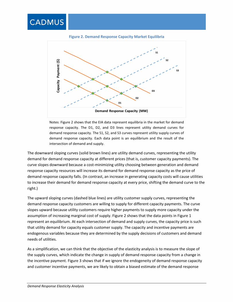
Figure 2 shows that each data point in Figure 1 represents an equilibrium between the supply decisions of individual utility customers and the utility’s demand for demand response capacity.
Demand Response Elasticity Analysis
Figure 2. Demand Response Capacity Market Equilibria
Capa
city
Pay
men
t ($)
Demand Response Capacity (MW)
S1
S2
S3
D1
D2
D3
Notes: Figure 2 shows that the EIA data represent equilibria in the market for demand response capacity. The D1, D2, and D3 lines represent utility demand curves for demand response capacity. The S1, S2, and S3 curves represent utility supply curves of demand response capacity. Each data point is an equilibrium and the result of the intersection of demand and supply.
The downward sloping curves (solid brown lines) are utility demand curves, representing the utility demand for demand response capacity at different prices (that is, customer capacity payments). The curve slopes downward because a cost-minimizing utility choosing between generation and demand response capacity resources will increase its demand for demand response capacity as the price of demand response capacity falls. (In contrast, an increase in generating capacity costs will cause utilities to increase their demand for demand response capacity at every price, shifting the demand curve to the right.)
The upward sloping curves (dashed blue lines) are utility customer supply curves, representing the demand response capacity customers are willing to supply for different capacity payments. The curve slopes upward because utility customers require higher payments to supply more capacity under the assumption of increasing marginal cost of supply. Figure 2 shows that the data points in Figure 1 represent an equilibrium. At each intersection of demand and supply curves, the capacity price is such that utility demand for capacity equals customer supply. The capacity and incentive payments are endogenous variables because they are determined by the supply decisions of customers and demand needs of utilities.
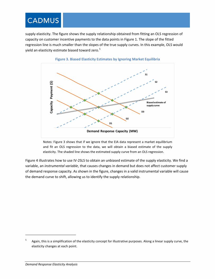
As a simplification, we can think that the objective of the elasticity analysis is to measure the slope of the supply curves, which indicate the change in supply of demand response capacity from a change in the incentive payment. Figure 3 shows that if we ignore the endogeneity of demand response capacity and customer incentive payments, we are likely to obtain a biased estimate of the demand response
Demand Response Elasticity Analysis
supply elasticity. The figure shows the supply relationship obtained from fitting an OLS regression of capacity on customer incentive payments to the data points in Figure 1. The slope of the fitted regression line is much smaller than the slopes of the true supply curves. In this example, OLS would yield an elasticity estimate biased toward zero.5
Figure 3. Biased Elasticity Estimates by Ignoring Market Equilibria
Capa
city
Pay
men
t ($)
Demand Response Capacity (MW)
S1
S2
S3
D1
D2
D3
Biased estimate of supply curve
Notes: Figure 3 shows that if we ignore that the EIA data represent a market equilibrium and fit an OLS regression to the data, we will obtain a biased estimate of the supply elasticity. The shaded line shows the estimated supply curve from an OLS regression.
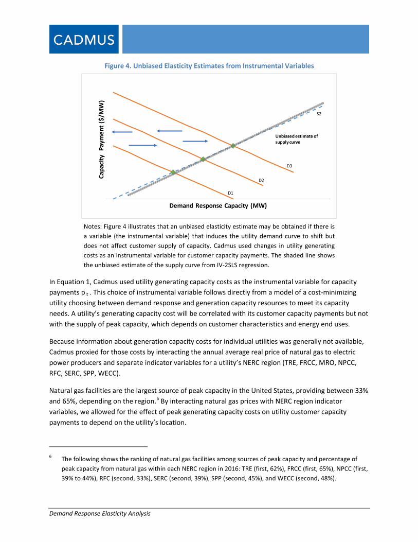
Figure 4 illustrates how to use IV-2SLS to obtain an unbiased estimate of the supply elasticity. We find a variable, an instrumental variable, that causes changes in demand but does not affect customer supply of demand response capacity. As shown in the figure, changes in a valid instrumental variable will cause the demand curve to shift, allowing us to identify the supply relationship.
5 Again, this is a simplification of the elasticity concept for illustrative purposes. Along a linear supply curve, the
elasticity changes at each point.
Demand Response Elasticity Analysis
Figure 4. Unbiased Elasticity Estimates from Instrumental Variables
Capa
city
Pay
men
t ($/
MW
)
Demand Response Capacity (MW)
D1
D2
D3
S2
Unbiased estimate of supply curve
Notes: Figure 4 illustrates that an unbiased elasticity estimate may be obtained if there is a variable (the instrumental variable) that induces the utility demand curve to shift but does not affect customer supply of capacity. Cadmus used changes in utility generating costs as an instrumental variable for customer capacity payments. The shaded line shows the unbiased estimate of the supply curve from IV-2SLS regression.
In Equation 1, Cadmus used utility generating capacity costs as the instrumental variable for capacity payments pit . This choice of instrumental variable follows directly from a model of a cost-minimizing utility choosing between demand response and generation capacity resources to meet its capacity needs. A utility’s generating capacity cost will be correlated with its customer capacity payments but not with the supply of peak capacity, which depends on customer characteristics and energy end uses.
Because information about generation capacity costs for individual utilities was generally not available, Cadmus proxied for those costs by interacting the annual average real price of natural gas to electric power producers and separate indicator variables for a utility’s NERC region (TRE, FRCC, MRO, NPCC, RFC, SERC, SPP, WECC).
Natural gas facilities are the largest source of peak capacity in the United States, providing between 33% and 65%, depending on the region.6 By interacting natural gas prices with NERC region indicator variables, we allowed for the effect of peak generating capacity costs on utility customer capacity payments to depend on the utility’s location.
6 The following shows the ranking of natural gas facilities among sources of peak capacity and percentage of
peak capacity from natural gas within each NERC region in 2016: TRE (first, 62%), FRCC (first, 65%), NPCC (first, 39% to 44%), RFC (second, 33%), SERC (second, 39%), SPP (second, 45%), and WECC (second, 48%).
Demand Response Elasticity Analysis
But a question is how do natural gas prices affect the cost of generating capacity costs? In regions with organized capacity markets, the price of natural gas would primarily affect the utilities’ cost of peak capacity through its effect on market entry and exit of power producers. Because natural gas-powered electricity-generating facilities can be built relatively quickly and inexpensively and fuel costs constitute between 60% and 80% of their levelized lifetime costs of operation,7 an increase in the natural gas price will raise operating costs and reduce incentives for market entry while increasing incentives for exit. In regions without organized capacity markets, high electricity prices provide scarcity rents to power producers, giving them incentives to enter the market and provide capacity.8 An increase in the natural gas price would reduce profitability and cause less entry and more exit of electricity producers.
Cadmus implemented the IV-2SLS estimation as follows.
• In the first stage, we regressed the natural logarithm of annual utility customer incentives on the natural logarithm of the annual price of natural gas to electric power producers interacted with a set of separate indicator variables for different NERC regions. The natural logarithm of annual natural gas prices to electric power producers served as the instrumental variable for utility customer capacity payments. The coefficients on the interaction variables indicate the elasticity of utility customer demand response capacity payments with respect to regional natural gas prices to electric power producers. The first stage regression also includes a separate time trend for each utility. Further details about this step in the analysis are presented in section 1.4.1.
• In the second stage, we regressed the utility’s annual potential demand response capacity on predicted annual customer incentives from the first-stage regression, an intercept, and a utility-specific time trend. The coefficient on predicted customer incentives was the elasticity of the customer supply of demand response capacity.
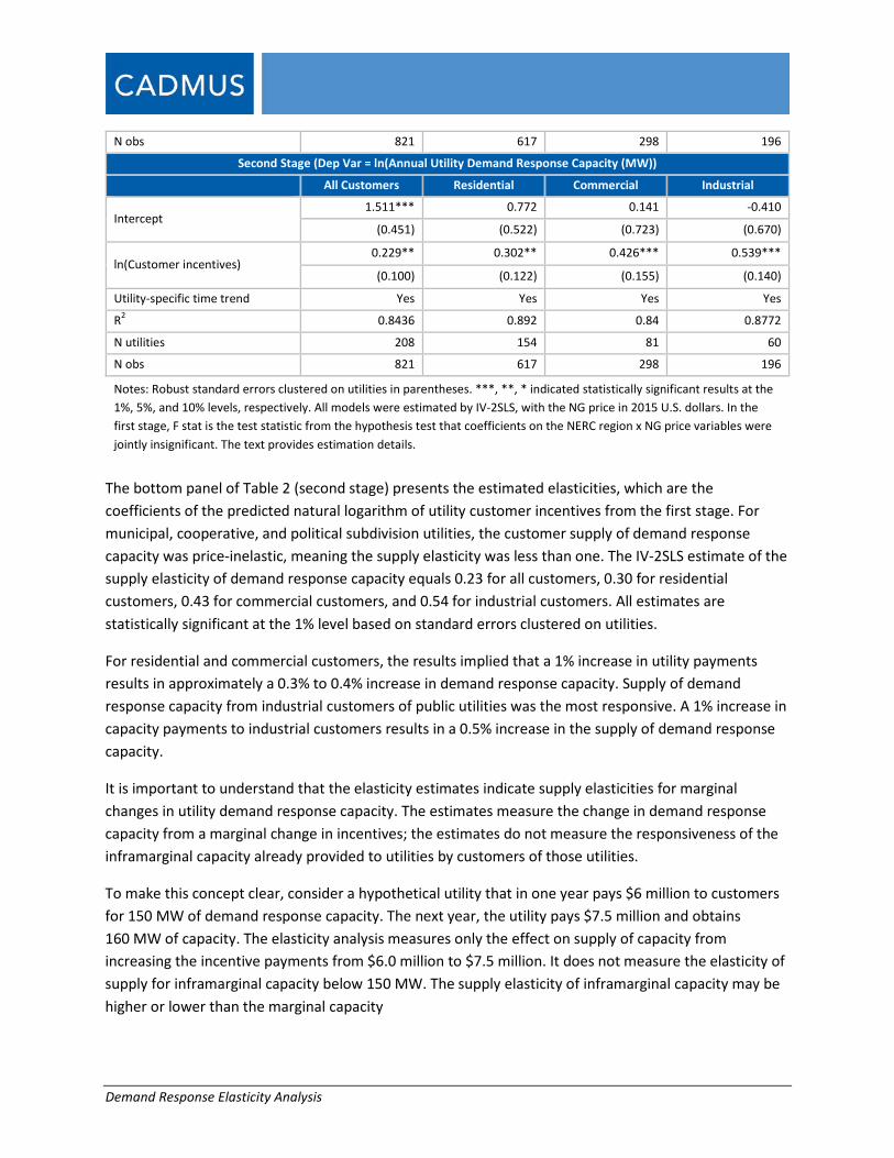
1.4.1 Demand Response Supply Elasticities for Public Utilities Table 2 shows results from the IV-2SLS estimation of the demand response supply elasticities for public utilities. The rows show the coefficient estimates with standard errors in parentheses, and the columns correspond to the separate models estimated for each customer segment and for all customers.
The top panel of Table 2 shows results from the first-stage estimation. The coefficients on the NERC region-natural gas price interaction variables indicate the elasticity of utility customer demand response capacity payments with respect to natural gas prices to electric power producers. For example, in the residential-sector first-stage regression, the FRCC x NG Price coefficient indicates that in the FRCC
7 United States Energy Information Administration. “Electric power sales, revenue, and energy efficiency Form
EIA-861 detailed data files.” Last modified August 31, 2017. Accessed October 20, 2017. https://www.eia.gov/electricity/data/eia861/.
8 Bushnell, James, Michaela Flagg, and Erin Mansur. Capacity Markets at a Crossroads. Prepared for Energy Institute at Haas, University of California, Berkeley. April 2017. Available online: https://ei.haas.berkeley.edu/research/papers/WP278Updated.pdf.

Demand Response Elasticity Analysis
region, a 1% increase in the price of natural gas to electric power producers results in a 0.64% increase in capacity payments to residential utility customers. In the SERC region, a 1% increase in natural gas price results in a 0.25% increase in capacity payments.
Cadmus found that thee first-stage regression results were as expected. The coefficients on the NERC region natural gas price instrumental variables in the first-stage regressions were positive and jointly statistically significant at the 1% or 10% level, as shown by the F statistics in Table 2. In general, natural gas price had its strongest impact on demand response capacity payments in NERC regions that depended most on natural gas facilities for supplying peak power—the Texas Reliability Entity (TRE), Florida Reliability Coordinating Council (FRCC), and SERC regions.9 This finding matched expectations.
Table 2. Demand Response Customer Supply Elasticities for Public Utilities First Stage (Dep var = ln(Annual utility customer incentives ($000))
Total Residential Commercial Industrial
Intercept 3.379*** 2.962*** 1.690* 3.818***
(0.433) (0.455) (0.794) (0.938)
FRCC x ln(NG Price) 0.639*** 0.615*** 2.736*** 1.021***
(0.123) (0.113) (0.531) (0.850)
MRO x ln(NG Price) 0.039 0.074 0.882* -0.768
(0.080) (0.086) (0.482) (0.671)
NPCC x ln(NG Price) 0.348 0.354 0.614
(0.295) (0.327) (0.441)
RFC x ln(NG Price) 0.084 0.180 0.012 -0.643
(0.102) (0.108) (1.686) (0.946)
SERC x ln(NG Price) 0.250*** 0.273*** 1.247* 0.773
(0.079) (0.084) (0.637) (0.517)
SPP x ln(NG Price) 0.234** 0.164 1.223** 0.971
(0.105) (0.140) (0.510) (0.628)
TRE x ln(NG Price) 0.425*** 0.647* 2.659*** 0.829*
(0.167) (0.361) (0.714) (0.457)
WECC x ln(NG Price) 0.136 0.114 1.018 0.862
(0.149) (0.113) (0.664) (0.636)
Utility-specific time trend Yes Yes Yes Yes
F stat 5.35 5.46 8.87 1.91
Prob(F > F Stat) 0.000 0.000 0.000 0.084
R2 0.763 0.744 0.822 0.838
N utilities 208 154 81 60
9 In 2016, natural gas facilities supplied 62% of peak capacity in the TRE (ERCOT), 65% in the FRCC, and 48% in
the WECC.
Demand Response Elasticity Analysis
N obs 821 617 298 196
Second Stage (Dep Var = ln(Annual Utility Demand Response Capacity (MW))
All Customers Residential Commercial Industrial
Intercept 1.511*** 0.772 0.141 -0.410
(0.451) (0.522) (0.723) (0.670)
ln(Customer incentives) 0.229** 0.302** 0.426*** 0.539***
(0.100) (0.122) (0.155) (0.140)
Utility-specific time trend Yes Yes Yes Yes
R2 0.8436 0.892 0.84 0.8772
N utilities 208 154 81 60
N obs 821 617 298 196
Notes: Robust standard errors clustered on utilities in parentheses. ***, **, * indicated statistically significant results at the 1%, 5%, and 10% levels, respectively. All models were estimated by IV-2SLS, with the NG price in 2015 U.S. dollars. In the first stage, F stat is the test statistic from the hypothesis test that coefficients on the NERC region x NG price variables were jointly insignificant. The text provides estimation details.
The bottom panel of Table 2 (second stage) presents the estimated elasticities, which are the coefficients of the predicted natural logarithm of utility customer incentives from the first stage. For municipal, cooperative, and political subdivision utilities, the customer supply of demand response capacity was price-inelastic, meaning the supply elasticity was less than one. The IV-2SLS estimate of the supply elasticity of demand response capacity equals 0.23 for all customers, 0.30 for residential customers, 0.43 for commercial customers, and 0.54 for industrial customers. All estimates are statistically significant at the 1% level based on standard errors clustered on utilities.
For residential and commercial customers, the results implied that a 1% increase in utility payments results in approximately a 0.3% to 0.4% increase in demand response capacity. Supply of demand response capacity from industrial customers of public utilities was the most responsive. A 1% increase in capacity payments to industrial customers results in a 0.5% increase in the supply of demand response capacity.
It is important to understand that the elasticity estimates indicate supply elasticities for marginal changes in utility demand response capacity. The estimates measure the change in demand response capacity from a marginal change in incentives; the estimates do not measure the responsiveness of the inframarginal capacity already provided to utilities by customers of those utilities.
To make this concept clear, consider a hypothetical utility that in one year pays $6 million to customers for 150 MW of demand response capacity. The next year, the utility pays $7.5 million and obtains 160 MW of capacity. The elasticity analysis measures only the effect on supply of capacity from increasing the incentive payments from $6.0 million to $7.5 million. It does not measure the elasticity of supply for inframarginal capacity below 150 MW. The supply elasticity of inframarginal capacity may be higher or lower than the marginal capacity
Demand Response Elasticity Analysis
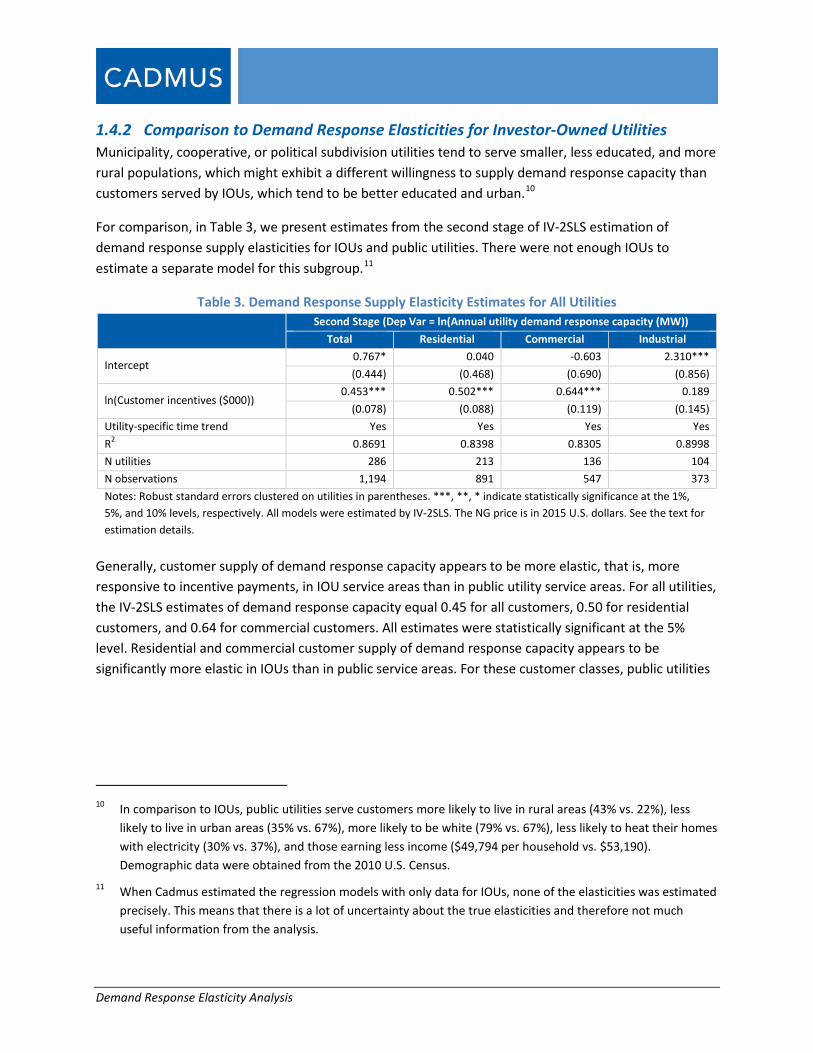
1.4.2 Comparison to Demand Response Elasticities for Investor-Owned Utilities Municipality, cooperative, or political subdivision utilities tend to serve smaller, less educated, and more rural populations, which might exhibit a different willingness to supply demand response capacity than customers served by IOUs, which tend to be better educated and urban.10
For comparison, in Table 3, we present estimates from the second stage of IV-2SLS estimation of demand response supply elasticities for IOUs and public utilities. There were not enough IOUs to estimate a separate model for this subgroup.11
Table 3. Demand Response Supply Elasticity Estimates for All Utilities
Second Stage (Dep Var = ln(Annual utility demand response capacity (MW))
Total Residential Commercial Industrial
Intercept 0.767* 0.040 -0.603 2.310*** (0.444) (0.468) (0.690) (0.856)
ln(Customer incentives ($000)) 0.453*** 0.502*** 0.644*** 0.189
(0.078) (0.088) (0.119) (0.145) Utility-specific time trend Yes Yes Yes Yes R2 0.8691 0.8398 0.8305 0.8998 N utilities 286 213 136 104 N observations 1,194 891 547 373 Notes: Robust standard errors clustered on utilities in parentheses. ***, **, * indicate statistically significance at the 1%, 5%, and 10% levels, respectively. All models were estimated by IV-2SLS. The NG price is in 2015 U.S. dollars. See the text for estimation details.
Generally, customer supply of demand response capacity appears to be more elastic, that is, more responsive to incentive payments, in IOU service areas than in public utility service areas. For all utilities, the IV-2SLS estimates of demand response capacity equal 0.45 for all customers, 0.50 for residential customers, and 0.64 for commercial customers. All estimates were statistically significant at the 5% level. Residential and commercial customer supply of demand response capacity appears to be significantly more elastic in IOUs than in public service areas. For these customer classes, public utilities
10 In comparison to IOUs, public utilities serve customers more likely to live in rural areas (43% vs. 22%), less
likely to live in urban areas (35% vs. 67%), more likely to be white (79% vs. 67%), less likely to heat their homes with electricity (30% vs. 37%), and those earning less income ($49,794 per household vs. $53,190). Demographic data were obtained from the 2010 U.S. Census.
11 When Cadmus estimated the regression models with only data for IOUs, none of the elasticities was estimated precisely. This means that there is a lot of uncertainty about the true elasticities and therefore not much useful information from the analysis.
Demand Response Elasticity Analysis
may face higher costs of obtaining peak capacity via demand response relative to IOUs. Only in the industrial sector was the elasticity of supply greater for customers of public utilities.12
1.4.3 Robustness of Elasticity Estimates The elasticity estimates remain robust to various changes in estimation approach. Table 4 presents results from the following robustness tests:
• Limiting the analysis sample to utilities with annual data for five or six years. The average utility in the sample has approximately four years of data.
• Estimating the first-stage regression with an expanded set of instrumental variables that includes whether the utility participated in one or more the following Regional Transmission Organization markets (CAISO, ERCOT, PJM, NYISO, SPP, MISO, ISONE, Other). A utility’s demand for demand response capacity and its incentives may have depended on its access to and participation in regional energy or capacity markets.
• Weighting each observation by annual utility electricity sector sales so that utilities with larger sales and peak demand receive more weight in the analysis.
• Including observations with positive demand response capacity but zero incentive payments in the analysis sample to allow for behavior-based demand response programs that do not provide capacity payments to customers.13
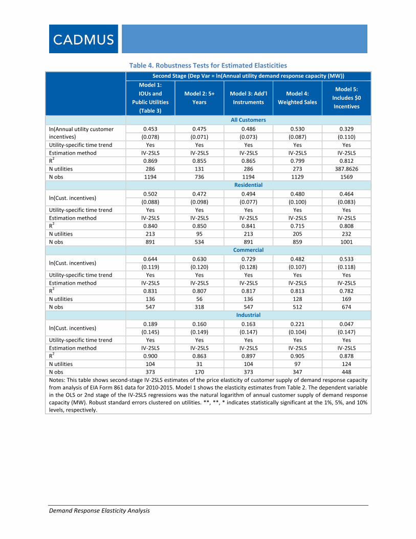
Each column of Table 4 corresponds to a different robustness test using regression. The table presents elasticity estimates for total, residential, commercial, and industrial demand response from the second-stage of IV-2SLS regression. The elasticity estimates in Table 4 should be compared to those in Table 3, since the robustness tests were estimated with the full sample of IOUs and public utilities. For ease of comparison, the first column in Table 4 presents the elasticity estimates from Table 3.
12 Industrial customer supply of demand response capacity may have been more elastic in public utility service
areas for several reasons. First, the analysis estimates elasticities for marginal, not inframarginal, demand response capacity. It could be that marginal capacity in IOU service areas is less elastic than in public utility service areas because demand response market penetration in the industrial sector is higher in IOU service areas. According to EIA, in 2015, existing industrial demand response capacity equals about 4% of utility system peak demand for utilities with industrial demand response capacity. (For comparison, the demand response market penetration for residential and commercial sectors is considerably lower, around 2%). In addition, EIA considers agricultural customers as industrial customers. Public utilities tend to serve more rural, agricultural areas, and it may be possible that agricultural customers have higher elasticities.
13 The natural logarithm of $0 is not defined. Cadmus estimated the elasticity models by first adding $1 to the annual customer incentive payments for all utilities in all years.

Demand Response Elasticity Analysis
Comparison of Model 1 to the other models shows that the demand response supply elasticity estimates are robust. The results are not sensitive to choices about sample selection, instrumental variables, or observation weights.
Demand Response Elasticity Analysis
Table 4. Robustness Tests for Estimated Elasticities
Second Stage (Dep Var = ln(Annual utility demand response capacity (MW)) Model 1: IOUs and
Public Utilities (Table 3)
Model 2: 5+ Years
Model 3: Add'l Instruments
Model 4: Weighted Sales
Model 5: Includes $0 Incentives
All Customers
ln(Annual utility customer incentives)
0.453 0.475 0.486 0.530 0.329 (0.078) (0.071) (0.073) (0.087) (0.110)
Utility-specific time trend Yes Yes Yes Yes Yes Estimation method IV-2SLS IV-2SLS IV-2SLS IV-2SLS IV-2SLS R2 0.869 0.855 0.865 0.799 0.812 N utilities 286 131 286 273 387.8626 N obs 1194 736 1194 1129 1569
Residential
ln(Cust. incentives) 0.502 0.472 0.494 0.480 0.464
(0.088) (0.098) (0.077) (0.100) (0.083) Utility-specific time trend Yes Yes Yes Yes Yes Estimation method IV-2SLS IV-2SLS IV-2SLS IV-2SLS IV-2SLS R2 0.840 0.850 0.841 0.715 0.808 N utilities 213 95 213 205 232 N obs 891 534 891 859 1001
Commercial
ln(Cust. incentives) 0.644 0.630 0.729 0.482 0.533
(0.119) (0.120) (0.128) (0.107) (0.118) Utility-specific time trend Yes Yes Yes Yes Yes Estimation method IV-2SLS IV-2SLS IV-2SLS IV-2SLS IV-2SLS R2 0.831 0.807 0.817 0.813 0.782 N utilities 136 56 136 128 169 N obs 547 318 547 512 674
Industrial
ln(Cust. incentives) 0.189 0.160 0.163 0.221 0.047
(0.145) (0.149) (0.147) (0.104) (0.147) Utility-specific time trend Yes Yes Yes Yes Yes Estimation method IV-2SLS IV-2SLS IV-2SLS IV-2SLS IV-2SLS R2 0.900 0.863 0.897 0.905 0.878 N utilities 104 31 104 97 124 N obs 373 170 373 347 448 Notes: This table shows second-stage IV-2SLS estimates of the price elasticity of customer supply of demand response capacity from analysis of EIA Form 861 data for 2010-2015. Model 1 shows the elasticity estimates from Table 2. The dependent variable in the OLS or 2nd stage of the IV-2SLS regressions was the natural logarithm of annual customer supply of demand response capacity (MW). Robust standard errors clustered on utilities. **, **, * indicates statistically significant at the 1%, 5%, and 10% levels, respectively.

Demand Response Elasticity Analysis
1.4.4 Impact of Customer Characteristics on Utility Customer Supply of Demand Response Capacity
How do the characteristics of utility customers affect their willingness to supply demand response capacity? Cadmus collected county-level demographic and housing characteristic data from the 2010 U.S. Census and mapped these data to utility service areas. We estimated the demand response supply elasticities for residential customers as a function of these demographic and housing characteristics to determine their influence on the willingness to supply capacity. The analysis sample included public utilities and IOUs. Only residential consumers were analyzed in this supplemental study.
Table 5 shows results from the OLS regressions of residential demand response capacity on customer incentives as a standalone variable and interacted with each of the following residential customer population characteristics:
• Average electricity consumption per customer
• Average peak electricity demand per customer in winter and in summer
• Percentage of customers in rural areas
• Percentage of customers in urbanized areas
• Percentage of customers attaining a bachelor degree or higher
• Percentage of the population older than 65
• Median income
• Percentage of homes that heated with gas
• Percentage of homes that heated with electricity
This report presents OLS estimates because the sample size was too small to obtain precise estimates of customer-characteristic impacts by IV-2SLS. When Cadmus estimated the models by IV-2SLS, none of the estimates of the coefficients on customer demographic characteristics that were interacted with customer incentives were precisely estimated. Because they ignore the endogeneity of demand response capacity and incentive payments, the OLS estimates are probably biased towards zero, that is, they are smaller in magnitude (closer to zero) than the true elasticities. Nevertheless, the estimates probably indicate the directional impact of demographic characteristics on the supply of demand response capacity. Because Cadmus rescaled the customer variables as sample standard deviations from the mean, the coefficients on the interaction terms should be interpreted as the elasticity effects of a one standard-deviation change in the customer variable.
Each column except the first in Table 5 corresponds to a different model for a customer characteristic. For example, the sixth model shows results for the effect of higher education on the elasticity of customer supply of demand response capacity.
In the sixth model, the row ln(Annual utility customer incentives) shows the estimate and standard error for the elasticity of supply of demand response capacity for residential customers with the percentage

Demand Response Elasticity Analysis
of college graduates equal to the average in the analysis sample of utilities. The estimated elasticity of supply for customers with the average college graduation rate equals 0.32. The row ln(Annual utility customer incentives) x Customer attribute shows the effect on the supply elasticity of a one standard-deviation change in the percentage of college graduates. A one standard-deviation change would increase the elasticity by 0.044 points. The last row of the table shows the sample standard deviation for percentage of college graduates is 0.08.
Besides education, several residential customer characteristics, including urban residency and heating fuel, were correlated with the supply of demand response capacity. A one standard-deviation change from the mean in the percentage of customers within urbanized areas (0.34) increased the demand response supply elasticity by 0.1 points. Rural customers were less willing to provide demand response capacity to utilities. Median income increased the elasticity of demand response supply, though only to a marginally significant degree. As expected, heating with electricity positively affected the elasticity of demand response capacity. A one standard-deviation change in the percentage of homes heated with electricity increased the demand response supply elasticity by 0.05 points.
When Cadmus ran a regression that included the urban, education, and electric heat variables, only the variables for urban residency (0.07 log points) and electric heat (0.04 log points) produced statistically significant effects. Because many customer characteristics, such as urban residency and education, are strongly correlated, it was not possible to simultaneously estimate their effects in a regression.

Demand Response Elasticity Analysis 19
Table 5. Demand Response Supply Elasticities as a Function of Customer Characteristics
Model 1: Annual
kWh per Customer
(MWh)
Model 2: Summer
Peak Demand
per Customer
(MW)
Model 3: Winter Peak
Demand per
Customer (MW)
Model 4: Rural (%)
Model 5: Urbanized Areas (%)
Model 6: Bachelor’s Degree (%)
Model 7: Age 65+ (%)
Model 8: Median
Income ($)
Model 9: Heat Gas
(%)
Model 10: Heat
Electricity (%)
ln(Annual utility customer incentives)
0.346*** 0.316*** 0.315*** 0.275*** 0.267*** 0.316*** 0.326*** 0.327*** 0.308*** 0.307***
(0.049) (0.046) (0.046) (0.041) (0.042) (0.047) (0.049) (0.047) (0.048) (0.046)
ln(Annual utility customer incentives) x Customer attribute
0.016 0.020 0.003 -0.087*** 0.095*** 0.044** -0.031 0.019 -0.051*** 0.053***
(0.025) (0.025) (0.023) (0.021) (0.022) (0.019) (0.030) (0.013) (0.019) (0.016)
Utility-specific time trend
Yes Yes Yes Yes Yes Yes Yes Yes Yes Yes
Estimation method OLS OLS OLS OLS OLS OLS OLS OLS OLS OLS
R2 0.852 0.848 0.847 0.859 0.860 0.854 0.852 0.852 0.856 0.857
N utilities 190 174 174 207 207 207 207 207 207 207
N obs 815 749 749 864 864 864 864 864 864 864
Customer attribute sample mean
12.4 0.0028 0.0026 0.347 0.473 0.256 0.220 51,236 0.532 0.323
Customer attribute sample standard deviation
3.1 0.0009 0.0011 0.221 0.337 0.080 0.042 10,597 0.184 0.208
Notes: Each model includes as regressors utility-specific time trends, ln(utility customer incentives) as a standalone variable and interacted with a utility customer attribute. Utility customer characteristics are rescaled as sample standard deviations from the sample mean. Robust standard errors clustered on utilities in parentheses. ***, **, * indicates statistically significant at the 1%, 5%, and 10% levels, respectively.
Demand Response Elasticity Analysis
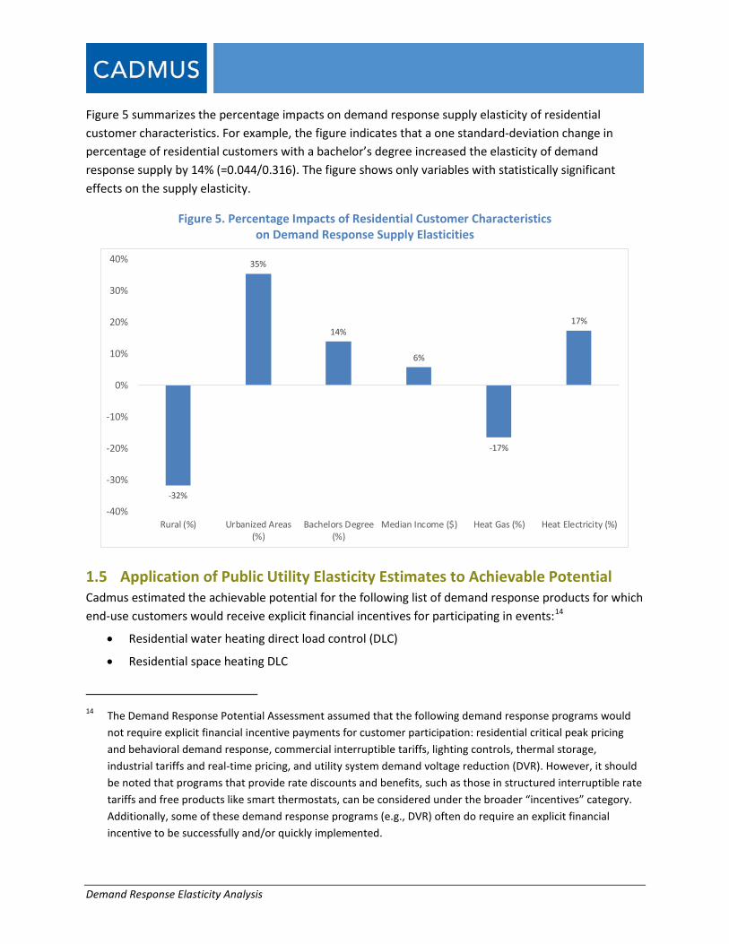
Figure 5 summarizes the percentage impacts on demand response supply elasticity of residential customer characteristics. For example, the figure indicates that a one standard-deviation change in percentage of residential customers with a bachelor’s degree increased the elasticity of demand response supply by 14% (=0.044/0.316). The figure shows only variables with statistically significant effects on the supply elasticity.
Figure 5. Percentage Impacts of Residential Customer Characteristics on Demand Response Supply Elasticities
-32%
35%
14%
6%
-17%
17%
-40%
-30%
-20%
-10%
0%
10%
20%
30%
40%
Rural (%) Urbanized Areas(%)
Bachelors Degree(%)
Median Income ($) Heat Gas (%) Heat Electricity (%)
1.5 Application of Public Utility Elasticity Estimates to Achievable Potential Cadmus estimated the achievable potential for the following list of demand response products for which end-use customers would receive explicit financial incentives for participating in events:14
• Residential water heating direct load control (DLC)
• Residential space heating DLC
14 The Demand Response Potential Assessment assumed that the following demand response programs would
not require explicit financial incentive payments for customer participation: residential critical peak pricing and behavioral demand response, commercial interruptible tariffs, lighting controls, thermal storage, industrial tariffs and real-time pricing, and utility system demand voltage reduction (DVR). However, it should be noted that programs that provide rate discounts and benefits, such as those in structured interruptible rate tariffs and free products like smart thermostats, can be considered under the broader “incentives” category. Additionally, some of these demand response programs (e.g., DVR) often do require an explicit financial incentive to be successfully and/or quickly implemented.
Demand Response Elasticity Analysis
• Residential central air conditioning (CAC) DLC
• Residential smart thermostats DLC
• Small commercial CAC DLC
• Commercial and industrial demand curtailment
• Agricultural Irrigation DLC
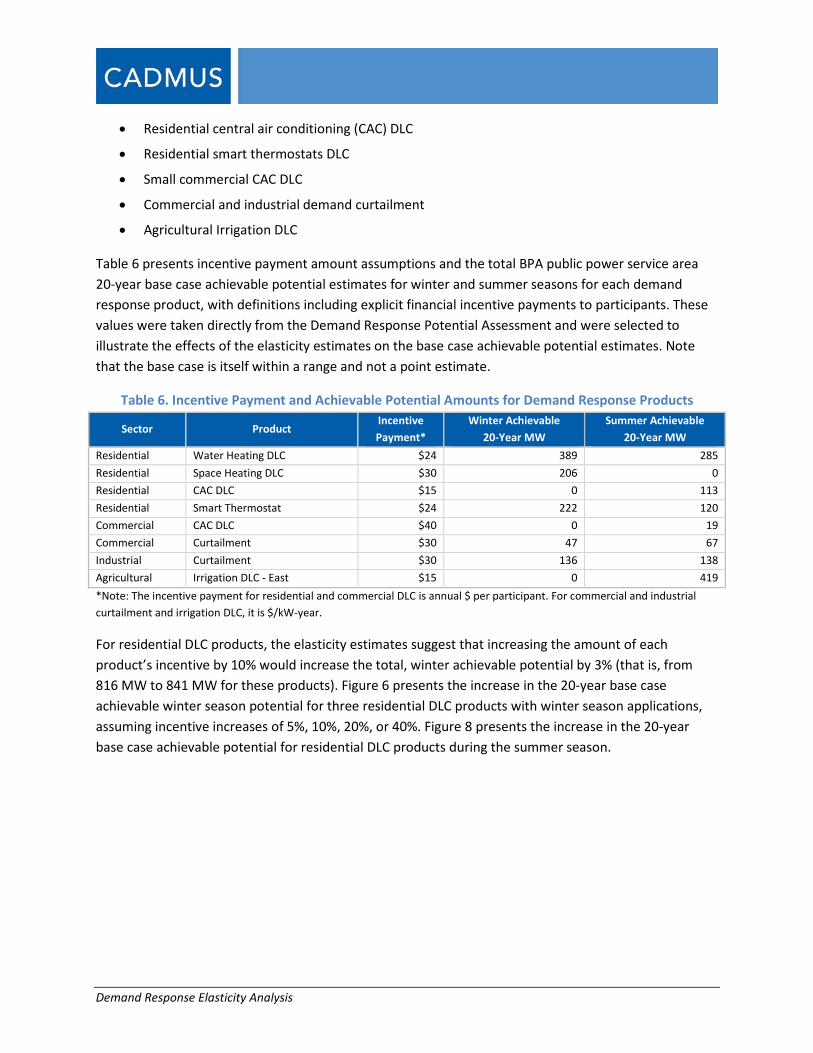
Table 6 presents incentive payment amount assumptions and the total BPA public power service area 20-year base case achievable potential estimates for winter and summer seasons for each demand response product, with definitions including explicit financial incentive payments to participants. These values were taken directly from the Demand Response Potential Assessment and were selected to illustrate the effects of the elasticity estimates on the base case achievable potential estimates. Note that the base case is itself within a range and not a point estimate.
Table 6. Incentive Payment and Achievable Potential Amounts for Demand Response Products
Sector Product Incentive Payment*
Winter Achievable 20-Year MW
Summer Achievable 20-Year MW
Residential Water Heating DLC $24 389 285 Residential Space Heating DLC $30 206 0 Residential CAC DLC $15 0 113 Residential Smart Thermostat $24 222 120 Commercial CAC DLC $40 0 19 Commercial Curtailment $30 47 67 Industrial Curtailment $30 136 138 Agricultural Irrigation DLC - East $15 0 419 *Note: The incentive payment for residential and commercial DLC is annual $ per participant. For commercial and industrial curtailment and irrigation DLC, it is $/kW-year.
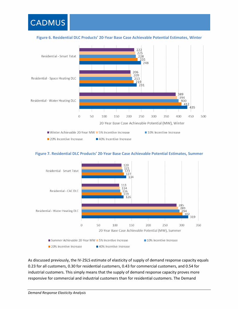
For residential DLC products, the elasticity estimates suggest that increasing the amount of each product’s incentive by 10% would increase the total, winter achievable potential by 3% (that is, from 816 MW to 841 MW for these products). Figure 6 presents the increase in the 20-year base case achievable winter season potential for three residential DLC products with winter season applications, assuming incentive increases of 5%, 10%, 20%, or 40%. Figure 8 presents the increase in the 20-year base case achievable potential for residential DLC products during the summer season.
Demand Response Elasticity Analysis
Figure 6. Residential DLC Products’ 20-Year Base Case Achievable Potential Estimates, Winter
Figure 7. Residential DLC Products’ 20-Year Base Case Achievable Potential Estimates, Summer
As discussed previously, the IV-2SLS estimate of elasticity of supply of demand response capacity equals 0.23 for all customers, 0.30 for residential customers, 0.43 for commercial customers, and 0.54 for industrial customers. This simply means that the supply of demand response capacity proves more responsive for commercial and industrial customers than for residential customers. The Demand
Demand Response Elasticity Analysis
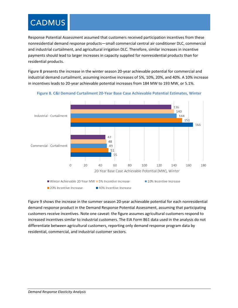
Response Potential Assessment assumed that customers received participation incentives from these nonresidential demand response products—small commercial central air conditioner DLC, commercial and industrial curtailment, and agricultural irrigation DLC. Therefore, similar increases in incentive payments should lead to larger increases in capacity supplied for nonresidential products than for residential products.
Figure 8 presents the increase in the winter season 20-year achievable potential for commercial and industrial demand curtailment, assuming incentive increases of 5%, 10%, 20%, and 40%. A 10% increase in incentives leads to 20-year achievable potential increases from 184 MW to 193 MW, or 5.1%.
Figure 8. C&I Demand Curtailment 20-Year Base Case Achievable Potential Estimates, Winter
Figure 9 shows the increase in the summer season 20-year achievable potential for each nonresidential demand response product in the Demand Response Potential Assessment, assuming that participating customers receive incentives. Note one caveat: the figure assumes agricultural customers respond to increased incentives similar to industrial customers. The EIA Form 861 data used in the analysis do not differentiate between agricultural customers, reporting only demand response program data by residential, commercial, and industrial customer sectors.
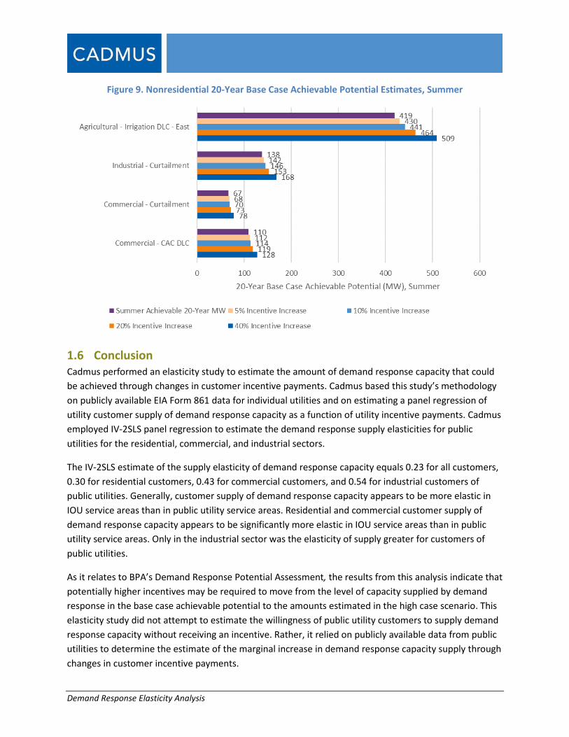
Demand Response Elasticity Analysis
Figure 9. Nonresidential 20-Year Base Case Achievable Potential Estimates, Summer
1.6 Conclusion Cadmus performed an elasticity study to estimate the amount of demand response capacity that could be achieved through changes in customer incentive payments. Cadmus based this study’s methodology on publicly available EIA Form 861 data for individual utilities and on estimating a panel regression of utility customer supply of demand response capacity as a function of utility incentive payments. Cadmus employed IV-2SLS panel regression to estimate the demand response supply elasticities for public utilities for the residential, commercial, and industrial sectors.
The IV-2SLS estimate of the supply elasticity of demand response capacity equals 0.23 for all customers, 0.30 for residential customers, 0.43 for commercial customers, and 0.54 for industrial customers of public utilities. Generally, customer supply of demand response capacity appears to be more elastic in IOU service areas than in public utility service areas. Residential and commercial customer supply of demand response capacity appears to be significantly more elastic in IOU service areas than in public utility service areas. Only in the industrial sector was the elasticity of supply greater for customers of public utilities.
As it relates to BPA’s Demand Response Potential Assessment, the results from this analysis indicate that potentially higher incentives may be required to move from the level of capacity supplied by demand response in the base case achievable potential to the amounts estimated in the high case scenario. This elasticity study did not attempt to estimate the willingness of public utility customers to supply demand response capacity without receiving an incentive. Rather, it relied on publicly available data from public utilities to determine the estimate of the marginal increase in demand response capacity supply through changes in customer incentive payments.