deformations of an elastic, internally constrained material. part 1: homogeneous deformations
TRANSCRIPT

Journal of Elasticity 29: 1-84, 1992. 1 © 1992 Kluwer Academic Publishers. Printed in the Netherlands.
Deformations of an elastic, internally constrained material. Part 1: Homogeneous deformations
M I L L A R D F. BEATTY ~ and M I C H A E L A. HAYES 2 ~ Department of Engineering Mechanics, University of Nebraska-Lincoln, Lincoln, NE 68588-0347, USA; 2Department of Mathematical Physics, University College, Dublin 4, Ireland
Received 29 June 1990
Akstract. The nonlinear elastic response of a class of materials for which the deformation is subject to an internal material constraint described in experiments by James F. Bell on the finite deformation of a variety of metals is investigated. The purely kinematical consequences of the Bell constraint are discussed, and restrictions on the full range of compatible deformations are presented in geometrical terms. Then various forms of the constitutive equation relating the stress and stretch tensors for an isotropic elastic Bell material are presented. Inequalities on the mechanical response functions are introduced. The importance of these in applications is demonstrated in several examples throughout the paper.
This paper focuses on homogeneous deformations. In a simple illustration of the theory, a generalized form of Bell's empirical rule for uniaxial loading is derived, and some peculiarities in the response under all-around compressive loading are discussed. General formulae for uni- versal relations possible in an isotropic elastic, Bell constrained material are presented. A simple method for the determination of the left stretch tensor for essentially plane problems is illus- trated in the solution of the problem of pure shear of a materially uniform rectangular block. A general' formula which includes the empirical rule found in pure shear experiments by Bell is derived as a special case. The whole apparatus is then applied in the solution of the general problem of a homogeneous simple shear superimposed on a uniform triaxial stretch; and the great variety of results possible in an isotropic, elastic Bell material is illustrated. The problem of the finite torsion and extension of a thin-walled cylindrical tube is investigated. The results are shown to be consistent with Bell's data for which the rigid body rotation is found to be quite small compared with the gross deformation of the tube. Several universal formulas relating various kinds of stress components to the deformation independently of the ma- terial response functions are derived, including a universal rule relating the axial force to the torque.
Constitutive equations for hyperelastic Bell materials are derived. The empirical work function studied by Bell is introduced; and a new constitutive equation is derived, which we name Bell's law. On the basis of this law, we then derive exactly Bell's parabolic laws for uniaxial loading and for pure shear. Also, from Bell's law, a simple constitutive equation relating Bell's deviatoric stress tensor to his finite deviatoric strain tensor is obtained. We thereby derive Bell's invariant parabolic law relating the deviatoric stress intensity to the corresponding strain intensity; and, finally, Bell's fundamental law for the work function expressed in these terms is recovered. This rule is the foundation for all of Bell's own theoretical study of the isotropic materials cataloged in his finite strain experiments on metals, all consistent with the internal material constraint studied here.

2 M.F. Beatty and M.A. Hayes
Table of contents
1. Introduction 2. The internal constraint 3. Geometry of the constraint
3.1. The invariant triangle 3.2. Kinematics of deformation 3.3. Generalized shear with normal stretch 3.4. An alternative geometrical description
4. The constraint reaction stress 5. Constitutive equations for an isotropic, elastic Bell material 6. Inequalities on the response functions
6.1. The OF-inequalities 6.2. The A-inequalities
7. The stress-free state 8. Uniaxial loading of a Bell material 9. Bell's stress tensor
9.1. Equilibrium equation and traction vector 9.2. Bell's empirical rule for uniaxial loading
I0. Principal directions and values of stress and stretch 10.1. Corresponding principal directions for a, T, and V 10.2. Corresponding principal values of a and V 10.3. Corresponding principal values of T and V
11. Universal relations 12. Determination of V for essentially plane problems 13. Pure shear and Bell's experiment
13.1. Bell's empirical relations for pure shear 14. Simple shear superimposed on a triaxial stretch
14.1. The universal relation for shear with triaxial stretch 14.2. Kinematics of deformation in the shear/stretch problem 14.3. The Bell stress in the shear/stretch problem 14.4. Traction relations in the shear/stretch problem 14.5, The Cauchy stress in the shear/stretch problem
15. Finite twist and axial stretch of a thin-walled tube 15.1. The thin-walled tube approximation 15.2. The small rigid rotation and related approximations 15.3. Stress in a thin-walled tube under finite twist and stretch
16. Isotropic hyperelastic Bell materials 17. Bell's law
17.1. Application of Bell's law to uniaxial loading 17.2. Application of Bell's law to pure shear 17.3. Bell's invariant parabolic law
18. Concluding remarks and summary of principal results 19. Additional recent developments Acknowledgement References
2 5 6 7 7
11 13 18 18 20 21 22 23 23 26 28 29 30 31 31 33 37 38 41 43 44 44 45 49 50 52 61 61 64 67 73 76 77 77 78 79 82 83 83
1. Introduction
T h i s p a p e r dea ls w i th the s t ruc tu re o f the stress t e n s o r and the d e f o r m a t i o n s
o f a ma te r i a l wh ich is sub jec ted to an in t e rna l cons t r a in t , ca l led the Bell
c o n s t r a i n t a f te r J a m e s F. Bell w h o first d rew a t t e n t i o n to it. Bell has r e p o r t e d
on an ex tens ive series o f e x p e r i m e n t s on v a r i o u s me ta l s c o n d u c t e d by h i m and

An internally constrained material 3
his students over many years. The principal results of these countless tests are summarized in his review article [1]. He noted in the experiments that large deformations of the materials always satisfied the rule tr V -- 3, where V is the left Cauchy-Green stretch tensor. This means that the sum of the principal stretches always equals three, a rule demonstrated in further detail in a more recent paper [2]. The purpose of our study is to explore the kinematical consequences of imposing this internal constraint and to determine its implica- tions for the form of the stress tensor for nonlinearly elastic materials. Further, we consider some deformations which satisfy the constraint and determine the corresponding stress and traction necessary to support these deformations. Some of the results are quite novel, even at variance with our physical intuition. We make theoretical predictions of the mechanical response of isotropic, nonlinearly elastic materials which tie in with the experimental observations of Bell for relatively large plastic deformations of a wide variety of isotropic metals.
The Bell constraint is introduced in §2 and its geometry is studied in §3. It is shown that the constraint describes a plane surface in principal stretch space, and it restricts all deformations to a region defined by an invariant equilateral triangle whose centroid is the undeformed state. Every deformation trajectory of a material point is thus described by a plane curve that begins at the centroid and remains within the invariant triangle. The region in the plane space of the two remaining independent principal invariants is subsequently constructed. The range of these important deformation variables is thus fixed by the boundary of this region. The boundary is described in physical terms, and the images in this region of some simple deformation paths identified in the invariant triangle are described. The geometrical regions studied here thus restrict all deformations kinematically possible in a Bell constrained material.
In considering the kinematical effects of the constraint, it is seen in §3 that the material volume in every deformation from an undistorted state of a Bell constrained material must decrease. Thus, isochoric deformations are not possible. Simple shear and simple torsion are two examples of deformation which are not possible. Many members of the well-known [6] five families of nonhomogeneous deformations possible in every incompressible, homoge- neous and isotropic elastic material are not possible in a Bell constrained material. For example, bending, stretching, and shearing of a rectangular block by surface tractions alone and isochoric inflation or eversion of a spherical shell are not possible.
A possible deformation is a generalized shear with normal stretch. It is seen in §3 that this is possible only with contraction normal to the plane of shear. In a sense, the normal contraction controls the amount of shear possible in the deformation.
The constitutive equation for the Cauchy stress for an isotropic Bell material is derived in §5. It is remarkable that no amount of all-around stress

4 M.F. Beatty and M.A. Hayes
applied to its undistorted state can deform a Bell material by a dilatation. Nevertheless, the material is not incompressible.
The now classical problem of what restrictions ought to be enforced on the response functions to ensure physically reasonable response is considered in §6. We propose for study the ordered forces inequalities and some empirical inequalities that we call ad hoc or A-inequalities. These play a principal role in the understanding of the solutions to problems.
Another possible homogeneous deformation is simple tension. It is seen in §8 that the longitudinal extensional strain is exactly one-half of the lateral contractive strain for all axial loads in a simple tension test of any Bell material whatever. Yet, we recall that there are no incompressible, Bell constrained materials.
Bell's stress tensor, introduced by Bell in [1] following the suggestion by Ericksen, is considered in §9; and the constitutive equation for an isotropic Bell material is displayed there. For a pure homogeneous deformation, it is seen that the principal Bell stress components are the principal forces. It turns out that the OF-inequalities for the principal Bell stress components in an isotropic Bell material are the analog of the Baker-Ericksen inequalities for the principal Cauchy stress components in an unconstrained or an incom- pressible, isotropic elastic solid.
In §10 it is seen that if the principal Cauchy stresses ti are all equal for an isotropic Bell material, it is possible that the undistorted material may deform differently in different directions. Thus, the principal extension ratios 2i may be such that 2~ = 22 :~ 23, and yet t~ = t 2 = t 3. The principal Bell stresses tr e, in this case, are such that tr~ = a2 ~ 0"3.
Since ¥ = B ~/2, it is usually tedious to determine V. However, the calcula- tions are simplified if V is known to be such that V~3 = V23 =0. Then following Ting [3], we present in §12 an easy method for the determination of V in terms of the deformation gradient tensor and B.
Pure shear is next considered in §13, and then in §14 we give a detailed analysis of the problem of simple shear superimposed on a triaxial stretch, the deformation introduced by Wineman and Gandhi [4] and by Rajagopal and Wineman [5]. The great variety of results possible in an isotropic, elastic Bell constrained material, including a peculiar effect of shear under pressure, is illustrated. The related problem of finite twist and extension of a thin-walled cylindrical tube is examined in §15. Kinematical relations are given for the thin-walled tube approximation, and afterwards small rigid rotation and related approximations are discussed. Our kinematical results are consistent with Bell's data, including his surprising empirical result that the rigid rotation of the principal axes of the left stretch tensor is quite small compared with the gross deformation of the tube. The stress in a thin-walled tube is then examined, and several universal formulas relating various kinds of stress

An internally constrained material 5
components to the deformation, independently of the material response functions, are derived. It is shown that the lateral tube surfaces may be traction free if and only if the rigid rotation of the coaxial principal directions for the Cauchy stress and the left stretch tensor is sufficiently small. For this case, we derive a universal rule relating the axial force to the torque in the otherwise finite twist and extension of the tube. Moreover, we find that this new rule is supported by Bell's data [18].
The various experiments by Bell [1, 2, 18] describe isotropic response of a variety of metals that undergo relatively large plastic deformation; and based upon an incremental theory of plasticity, Bell has shown that the material response is consistent with the constraint tr V = 3 and also may be character- ized by a certain work function, which Bell sometimes calls the "strain energy" function. Thus, if no unloading occurs, such response may be considered typical of an isotropic, hyperelastic solid. Therefore, with this motivation, in §16 isotropic, hyperelastic Bell materials are considered and their general constitutive equation displayed. Assuming the validity of our A-inequalities, we prove that for an isotropic, hyperelastic solid our strain energy must increase as its invariant arguments decrease from their maximum values in the undistorted state. More specifically, we next recall the special work function for which Bell [1] has shown all of his tests to be consistent. Using it to define and investigate a similar class of isotropic, hyperelastic materials, in §17 we derive precisely Bell's parabolic law for uniaxial loading, precisely Bell's parabolic law for pure shear, and also precisely Bell's parabolic law relating the deviatoric stress intensity to the corresponding strain intensity reported in his experiments. It is most important to emphasize again, how- ever, that Bell's studies deal with finite strain plasticity theory, whereas the present study focuses on nonlinearly elastic deformations of isotropic solids characterized by a similar work function; and no immediate association with plasticity is presently intended.
In this primary study, we have introduced a kinematical constraint discov- ered in the context of finite strain plasticity of metals and have explored its consequences within the framework of finite elasticity theory. Our results, therefore, must be viewed in this context. It is nonetheless remarkable that our theoretical results predict and concur accurately with the great body of Bell's experimental data.
2. The internal constraint
Let xo and x denote the respective reference and current configurations of a body ~. Relative to a common Cartesian frame ~0 = {O; ek}, the position vector x(X, t) from the origin O is the place in x at time t occupied by the

6 M.F. Beatty and M.A. Hayes
material point P whose place was X = X(P, to) in x 0 at the instant to. The deformation gradient F = dx/dX has the polar decomposition
F = R U = VR, J = det F > 0 , (2.1)
in which U and V are positive, symmetric stretch tensors and R is a proper
orthogonal tensor. We recall also the symmetric deformation tensor
B -= V 2 = FF r (2.2)
and the velocity gradient tensor
L _= lZF_t ~v - - ~ = ~ x D + W , (2.3)
with v(x, t) =/~(X, t), and D = D r and W = - W r are the symmetric and skew
parts of L. The superimposed dot denotes the usual material time derivative.
An internal constraint imposed on the deformation (2.1) is a scalar valued kinematical relation defined by a smooth function y(F) = 0. However, applica- tion of the principle of material frame indifference [6] reveals that ~,(F) must
have the reduced form 7(U) = ~,(RrVR) = 0. It follows that if 7 is a function
of the principal invariants of U, then ~,(U) = ~(V) = 0. The present study concerns a class of materials for which the internal constraint
y(V) = I v - 3 = t r Y - 3 = 0 (2.4)
holds for all deformations of :~. Bell [1, 2] has demonstrated the consistency of the rule (2.4) with countless data obtained from a variety of experiments on
the finite strain of metals. Therefore, (2.4) is called the Bell constraint, and a material that respects this rule is named a Bell material.
With the aid of (2.1)2, (2.3) and the orthogonality condition R R r = RrR = 1, it can be shown that the material time derivative of (2.4)
yields the equivalent constraint equation
~;(V) = tr ~" = tr(VD) -= V" D = 0. (2.5)
It is helpful to recall here that S = RR r is a skew tensor and tr[(W + S)V] = 0.
3. Geometry of the constraint
In this section, the Bell constraint is examined in detail. The results are novel. It is shown that the volume in every deformation of a Bell material must

An internally constrained material 7
decrease; therefore, isochoric deformations are not possible. We briefly exam- ine in §3.3 a generalized shear with normal stretch, a deformation which is compatible with the constraint. Even so, we find that the transverse stretch must be a contraction normal to the plane of shear. It is then shown in §3.4 that every Bell material behaves in small deformations like an incompressible material whose Poisson function in every simple extension, however great, has the constant value 1/2, yet the material can support no volume preserving strain whatever. All results presented in this section are purely kinematical results that respect the constraint (2.4), and hence they are independent of the specific mechanical response of the material.
3.1. The &variant triangle
We begin by observing that the kinematic constraint (2.4) describes a plane surface
2t + 22 + 23 - 3 = 0 (3.1)
in the 2-space of the principal values of V. Hence, (3.1) restricts the positive principal stretches 2 k to values in the plane region bounded by three lines 2i + 2j = 3, i ¢ j = 1, 2, 3. These lines form the equiangular, triangular base of an equilateral tetrahedron of edge length 3. This is illustrated in Fig. 1. Therefore, the region described by the invariant plane (3.1) with 0 < 2k < 3 is named the invariant triangle.
The position vector k = 2~ Ik of a point in the invariant plane has magnitude 1~1 = 11/2= (tr V2) ~/2. Hence, the first invariant of B is the squared distance from the origin F of the principal frame ff = {F; 1~ } to a point in the invariant triangle. The centroid of the invariant triangle is the undistorted state (1, 1, 1); it is the point in the invariant plane nearest to F. Every deformation trajectory at a material point must be described by a plane curve ~ that begins at the centroid of the invariant triangle. The principal vector k traces a plane path 5 a whose constant binormal vector is b = (1/x/~)( 1, l, 1), the unit normal vector to the invariant plane. Thus, in geometrical terms, the constraint (3.1) is equivalent to the invariance of the orthogonal projection of k upon b, that is, ~. • b = x/~, the height of the tetrahedron. Some particular deformation paths are examined next.
3.2. Kinematics of deformation
The lines drawn from its vertices through the undistorted state are perpendic- ular bisectors of the sides of the tetrahedral triangle. These unique principal deformation trajectories are states of equibiaxial stretch. One such line is the

M.F. Beatty and M.A. Hayes
Invariont Trion(.
XI+X2+XS=5
Xl+X3=
/ /
O)
,(X I, ~ _ ~ .
," ./
v i¢ " I / , , ( I ,1 ,1) 45 °
l ~ ~ _ ~ _ _ _ _ _ P - - - - - - ~ I
/ ~ o , o , o ) ' ~ ~
+k3=5
(0,~,,0)
'kl+X~=~,
Fig. I. Geometry of the internal constraint (3.1).
path 2~ = ~ . 2 , 2~,1 +/~'3 = 3 shown in Fig. 2. Clearly, if at most one principal stretch 2i = 1, then 2j + 2k = 2, i, j, k ¢ . These trajectories of plane stretch are lines parallel to the sides of the invariant triangle, and thus share only the undistorted state with any line of equibiaxial deformation. The plane stretch path 21 + 22 --- 2, 23 = 1 is perpendicular to the trajectory of equibiaxial stretch in Fig. 2, for example. Hence, an equibiaxial plane stretch and, of course, a nontrivial uniform all-around contraction or expansion are impossible in any Bell material. The same results follow easily from (3.1).
We notice that in an equibiaxial deformation with normal stretch 23 = 2, say, (3.1) yields 21 = (3 - 2)/2; and the change in the material volume V from its value Vo in x 0 is readily determined by V/Vo =I l l v = ~.1,~.2)~3 = ~.(3 - 2 ) 2 / 4 ~< 1 for all 2 e (0, 3). Therefore, in every equibiaxial deformation from an undis-

An internally constrained material 9
),3
),1 + ),3 = 5
/
A
I
0,5)
+ ) ,3=3
Ext(
_ _ / Compressional
/
/ / -- ~ , 0 )
5,0,0)
).1+).2= 2, X3 = I Plane Stretch
(0 ,2 ,1 )
XlX2= l , ks= l Simple Shear , jc _-- •
(o ,5 ,o ) x z
2)` i+)`3=3, ). i =). 2
Equibiaxial Stretch
h i + k 2 = 3
X I
Fig. 2. Geometrical description of a plane stretch, an equibiaxial stretch and a simple shear. Note that an equibiaxial plane stretch and a simple shear are impossible in a Bell constrained material. Equibiaxial extensional deformation exhibits lateral contraction, and compressional, lateral expansion, as usual.
torted state, the material volume of a Bell constrained material decreases in the manner illustrated in Fig. 3.
In fact, under the constraint (3.1), it can be shown more generally that the functionf(21, 22, 23) = I I I v = 2] 2223 has its greatest value 1 at the undistorted state; and therefore I I I v < 1 for all nontrivial deformations of a Bell material. Hence, the material volume in every deformation of a Bell material must decrease: V < Vo. Indeed, Bell [2, 7] recognized and confirmed in a variety of experiments by himself and others the rule of decreasing volume under finite strain. Moreover, it can be shown that the function g(2], 22, ) ,3)- = IIv = 2]22 + 2223 + )-3 2] also has its absolute maximum value 3 at the undis- torted state. Thus, in every deformation of a Bell material, the principal

10 M.F. Beatty and M.A. Hayes
1.25 t~...Undistorted State
II q' ~.. -~)Inflection Point
:~
0 I ~
0 I ~ 3 S~r~t~h, X~ (0,3)
~ig. ~. ~ o l u ~ ~du~tion in an ~quibia~iai deformation as ~ functio~ of the n o d a l axial stretch ~ ~or both a~ial lengthening (~ ~ l) and shortening (~ ~ 1) o~ th~ body.
invariants must respect the rules L
I v = 3 , IIv<~3, I I Iv=V/Vo<~l . (3.2)
We have seen that the equalities in the last two results may hold only in the undistorted state. Therefore, no isochoric deformations are possible in a Bell material. The surface 212223 = 1 shares only the unique tangent point (1, 1, 1) with the invariant plane. In particular, a simple shear is impossible. It is seen in Fig. 2 that a simple shear for which 2 3 = 1 and 213.2 = 1 has a hyperbolic principal deformation path which is not in the invariant plane. It is evident, of course, that incompressible Bell materials do not exist.
In consequence, familiar important families of nonhomogeneous, isochoric deformations known to be controllable in every incompressible, homogeneous
1 For comparison, we note that in every deformation of an incompressible material the principal invariants mus t satisfy the relations Iv ~> 3, I1 v >~ 3, l l l v = 1.

An &ternally constrained material 11
and isotropic elastic material [6] cannot be effected in any material con- strained by (3.1). Specifically, the isochoric deformations described as Family 1: bending, stretching, and shearing of a rectangular block; Family 2: straight- ening, stretching, and shearing of a sector of a hollow cylinder; and Family 4: inflation or eversion of a sector of a spherical shell, cannot be produced in a Bell material. Of course, this rule does not preclude existence of possible special anisochoric deformations that may be similar to these. Among the familiar classes, however, only Family 3: inflation, bending, torsion, exten- sion, and shearing of an annular wedge; and Family 5: inflation, bending, extension, and azimuthal shearing of an annular wedge, are not identically isochoric deformations and thus remain as potential candidates for study. On the other hand, pure torsion, a special isochoric member of Family 3, is impossible in any Bell material. Further discussion of nonhomogeneous de- formations is reserved for Part 2 of this work. An example of a kinemati- cally admissible homogeneous deformation possible in every Bell material is described next.
3.3. Generalized shear with normal stretch
Let us consider a nonisochoric deformation for which the principal stretches satisfy
2~22=1, 23=/~. (3.3)
An example is a simple shear of amount K with normal stretch #; this is defined by
x = X + K Y , y = Y , Z=l~Z, (3.4)
in which (x, y, z) is the coordinate image in x of the point in Xo at (X, Y, Z) in a common rectangular Cartesian frame. Hence, (3.3) describes a general- ized shear with normal stretch. Use of (3.3) in (3.1) yields the constraint equation
/~ = 3 - (21 + 22) = 3 - 21 . (3.5)
Since 0 < p = I I I v ~< 1 for every Bell material, the equality holding only in the undistorted state, a generalized shear with normal stretch can occur only with transverse contraction normal to the plane of shear. The extent of the contraction is determined by the degree of shear in accordance with (3.5). We see also that 1 < IIv = 1 + 3# - t~ 2 <~ 3.

12 M.F. Beatty and M.A. Hayes
I f # is a specified parameter and we order 21 > 3.2, then
, - . - ~ -t- - 1 , (3.6a)
and
22 - 21 2 - 1. (3.6b)
Thus, in a Bell material, the extent of a generalized shear may be controlled by application of forces that limit the degree of the normal contraction. In this sense, the transverse deformation may control the amount of shear possible in a generalized shear with normal stretch. I f the deformat ion is constrained by
forces so that /x = 1, for example, the deformat ion (3.3) is isochoric, and
hence no shear whatever can occur. In fact, (3.6) yields 21 = 22 = 1.
The deformat ion trajectory for a generalized shear with normal stretch is
shown in Fig. 4. The arc OAB in the invariant plane is described by (3.6a) and
)'3
,3) Trajectory of Equibioxiol Stretch kl=X2,2kl+X3=5
Trajectory of Plane Stretch XI+ k 2 = 2~';':
(3,0,0)
Deformation Trajectory in Generalized Shear with Normal Contraction,
klX2 = I, X3= F
XK_<_O__\. C . . . . k2
. I , I • ~ ;
k I +k 5=3, k 3--0
/ ~< ~-C-. 3-_~_~. o>., :_~ kl
Fig,. 4. Deformation trajectory of a general shear with normal stretch shown in the invariant plane. The values of K describe the same path for a simple shear of amount K and normal stretch ,l 3 = #.

An internally constrained material 13
(3.6b). When the roles of 2~ and 22 are reversed, the deformation path is traced by the arc OCD. A simple shear with normal stretch defined by (3.4) is an example of a generalized shear for which the curves OAB and OCD correspond to the symmetry in the amount of shear K when the direction of shear is reversed. The Bell constrained path of a simple shear with normal stretch in Fig. 4 is to be compared with the impossible simple shear trajectory shown in Fig. 2.
Notice also that the equibiaxial path on which 2~ = 22 is a line of symmetry for the path of generalized shear with normal stretch; and the other equibiax- ial lines for which 2~ = 43 and 42 = 43 intersect this path at the points A and
1 C where/~ = ~. Moreover, for the circumstances shown in Fig. 4, it is seen that a normal expansion occurs only for points in the region above the deforma- tion path of plane stretch, while the path of generalized shear lies entirely within the region of normal contraction beneath it.
It can be shown that the points A and C also are transition points at which the maximum orthogonal shear component of V changes. At the point A it changes from
(Vi2)max ~ ~ = ½V/(1 - ]./)(5 - ]./) (3.7a)
when ½ </~ ~< 1, to
~ 3(1 -/~) + ¼x/( 1 _/~)(5 -/~) (3.7b) (Vl3)max ~ = T
1 when 0 </~ < 21-, the two being equal to ~ at/~ = 2. The former occurs in the 12-plane of shear whereas the latter occurs in the 13-plane normal to it. Hence, the maximum orthogonal shear component of V need not occur in the plane of the generalized shear when the normal contraction is severe. A similar thing occurs at C when the roles of 2~ and 22 in (3.6a) and (3.6b) are reversed and (3.7b) is replaced by (V23)max.
3.4. An alternative geometrical description
The geometry of the constraint (3.1) also may be described in terms of Bell's finite strain tensor E defined by
E = V - 1. ( 3 . 8 )
We first note that E and V have common principal directions and their respective principal values Ek and 2k are related by E~ = 2 ~ - 1. Let

14 M.F. Beatty and M.A. Hayes
k o = (1, 1, 1). Then F = gkl k =--~,- ~'0, the principal engineering strain vector, is the position vector from the undistorted state O, the origin of the E-space in the invariant plane, to a point on the principal deformation trajectory described in terms of the principal engineering strains Ek.
The principal invariants of E and V are related by
Iv = 3 + I ~ , I I v = 3 + 2 I E + I I r , (3.9a)
AV - - = I I I v - 1 = IE + II~ +IIIr , (3.9b) Vo
in which A V = V - V0 denotes the change of material volume. The first of (3.9a) shows that the constraint (3.1) may be written as
I E = t r E = E ~ + E 2 + E 3 = O for - 1 <Ek <3; (3.10)
and in view of (3.2), (3.9a)2 shows that 0 ~< --lie ~< 3. It may be seen that the distance from O to a point on the principal deformation trajectory in E-space is
Irl = (tr E 2) ,/2 = ( _ 2IIt ) ~/2. (3.11)
In a plane strain for which E3--0, the constraint (3.10) requires that E~ = -E2 . For an equibiaxial strain for which E1 = E2, we have 2E~ = - E 3. Hence, in a simple extension with stretch ~'3 = '~, every Bell material has a constant Poisson function v ( 2 ) - - - E ~ / E 3 = 1/2, as noted by Beatty and Stalnaker [8]. On the other hand, as emphasized by Bell [l] and demonstrated in our examples above, the constraint (3.10) is not an incompressibility constraint in finite strain. Thus, every Bell material behaves in small deforma- tions like an incompressible material whose Poisson function in every simple extension, however great, has the constant value Vo = 1/2, but the volume actually decreases in every deformation. We note that our earlier remarks concerning the maximum orthogonal shear component of V in a generalized shear with normal stretch apply at once to the corresponding orthogonal shear component of Bell's strain tensor E.
Use of (3.2) in (3.9) shows only that 0 ~< - I IE ~< 3 and IIIE <~ -IIE. To determine more precisely the range of the deformation variables IIr and III~, hence also those in (3.2), we recall the Cayley-Hamilton equation for E. With the aid of (3.10), we have
E 3 + IIEE -- I I Ir l = 0. (3.12)
An &ternally constrahted material 15
Therefore, the corresponding characteristic equation has three real roots if and only if
( III~'~ 2 I" II~'~ 3 T ) + ~ T ) ~<0, (3.13)
equality holding when and only when at least two principal values E~ of E (or 2k of V) are equal. We recall from (3.10)~ or (2.4) that the particular state for which all three proper values of E (or V) are equal is the trivial undeformed state. Hence, it is seen again that a Bell constrained material cannot support an all-around expansion or contraction, regardless of the nature of the loading.
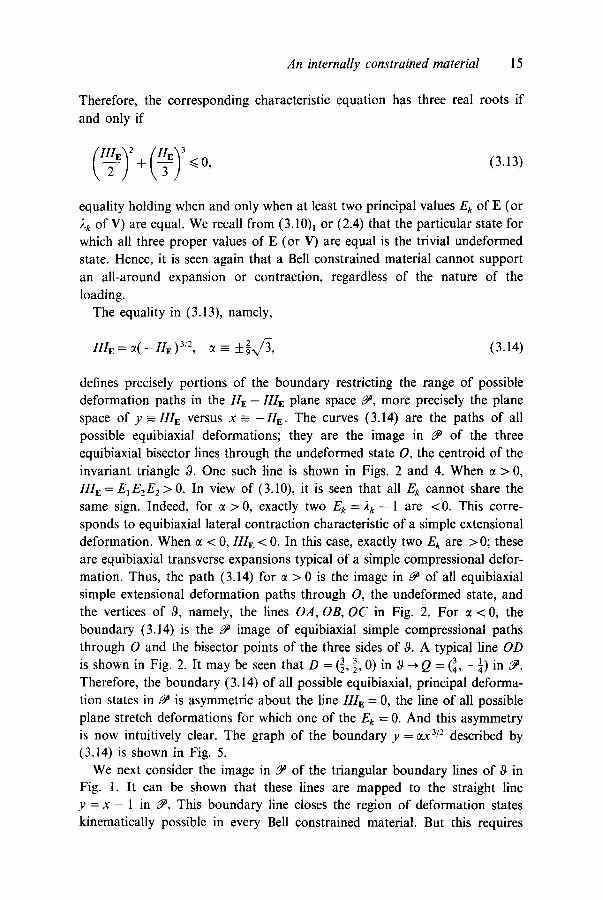
The equality in (3.13), namely,
2 I I l ~ = c t ( - - I I ~ ) 3/2, ~ = +~x/~, (3.14)
defines precisely portions of the boundary restricting the range of possible deformation paths in the I I E - I I l E plane space ~, more precisely the plane space of y =- III~ versus x =- - I I ~ . The curves (3.14) are the paths of all possible equibiaxial deformations; they are the image in ~ of the three equibiaxial bisector lines through the undeformed state O, the centroid of the invariant triangle 9. One such line is shown in Figs. 2 and 4. When a > 0, III~ = E~EEE 2 > 0. In view of (3.10), it is seen that all Ek cannot share the same sign. Indeed, for ~ > 0, exactly two E k = ) , k - 1 are <0. This corre- sponds to equibiaxial lateral contraction characteristic of a simple extensional deformation. When ~ < 0, III~ < 0. In this case, exactly two Ek are > 0; these are equibiaxial transverse expansions typical of a simple compressional defor- mation. Thus, the path (3.14) for ~ > 0 is the image in ~ of all equibiaxial simple extensional deformation paths through O, the undeformed state, and the vertices of 9, namely, the lines OA, OB, OC in Fig. 2. For ~t < 0, the boundary (3.14) is the ~ image of equibiaxial simple compressional paths through O and the bisector points of the three sides of 9. A typical line OD is shown in Fig. 2. It may be seen that D = (z 3-, I, 0) in ~ ~ O = (~, -41-) in ~ . Therefore, the boundary (3.14) of all possible equibiaxial, principal deforma- tion states in ~ is asymmetric about the line III~ = 0, the line of all possible plane stretch deformations for which one of the E~ = 0. And this asymmetry is now intuitively clear. The graph of the boundary y = ~x 3/2 described by (3.14) is shown in Fig. 5.
We next consider the image in ~ of the triangular boundary lines of ~ in Fig. 1. It can be shown that these lines are mapped to the straight line y = x - 1 in ~. This boundary line closes the region of deformation states kinematically possible in every Bell constrained material. But this requires

16 M.F. Beatty and M.A. Hayes
~. Common y=TTT~ ==+ ~ tanqent at P y P = ( 3 , 2 )
Y = a X 3 / 2 , a > O ~
Simple extensional type ~ equibioxiol deformations// ~ ~
c ~ ~ " ~ - ~ . / ..Y=X-I Plane stret . . . . - ~ / ~ l l o o u n a a r y
o , ,
o --
/ -
y=ax 312, a<O Simple compressionol type equibioxiol deformotions
Fig. 5. Graphical description of` the ~c~ion of" all kincmat~cally possible dcf"onnatJons Jn the plane ~p~cc of" the p~nc~pa] ~n~afiants o~ E plottc~ as IH~ ~ersus -H~.
further description. In particular, the line )`1 + )`3 = 3, ),2 = 0 in Fig. 1 is the line E l + E 3 = 1, E 2 = - 1 in E-space. Thus, I I I E = - E l E 3 and l iE=
E2(E1 + E3) + EIE3 = - I I I E - 1, that is, IIIE = ( - - l iE ) -- 1. The vertex points (0 ,0 ,3) and (3 ,0 ,0) in Fig. 1 map to ( - 1 , - 1 , 2 ) and ( 2 , - 1 , - 1 ) in E-space, and their common image in ~ is the point P in Fig. 5, also the image of the remaining vertex point of 9. The point E at (2, 0, 1) on the side AB of ~ in Fig. 2 must map to a point on the line QP in Fig. 5. Since E also is a point on a line of plane stretch )̀ 3 = 1, hence E 3 = 0 , we have IIIE = O, --liE = 1. Therefore, the image in ~ of the point (2, 0, 1) in ~ is the point (1, 0) at R in Fig. 5. The line OR is the image in ~ of the three lines through O and parallel to the sides of 9, the deformation paths of all possible plane stretches. This completes our construction of the boundary of the region in the l i e - IIIE plane space ~ of all deformation paths possible in a Bell constrained material.
All end points and connecting, simple deformation paths in the invariant triangle 9, which includes the specific paths described in the foregoing construction, are illustrated and labeled completely in Fig. 6. We note that EB = equibiaxial and PS = plane stretch; the shorter EB segments are com-

XI+X 3"3, ~'2-"
An internally constrained material
A(O,O,3)
~ , . ~ X 2 +X3-- 3, X~--0
17
,0,- - } L G (0,-- , - -) (.~.~ 3 PS E PS ~ 3
0,~,1)
/= ~~l~,.,.Jd~ ~
~ : Z ~ ~~ ~~ ~ ~ ~,o .o, ~(3,o,o) (e,~,o) / o ~,z,o~ ~ - '~
~.~.o~ x X~+X~-3, X3-O
Fig. 6. Equibiaxial (EB), plane stretch (PS), and ultimate compressional (boundary line) defor- mation paths in the invariant triangle. The EB subscript C denotes compressional, E extensional type deformations normal to the plane of equibiaxial stretch.
pressional (C), the longer ones extensional (E), as described earlier. To illustrate the mapping of paths in ~ - , ~ explored above, a sequence of possible deformation paths traced in ~9 in Fig. 6 and its corresponding image traced in ~ in Fig. 5 is provided below:
Path in ~ Path in ~
O A --, H ~ G or or or or or ~ ~ F - - * C - ~ O , O ~ P - * R - - * Q ~ R - ~ P ~ O ~ ~ ~ ~ ~ ~
0 0 0 0 0 0
Hence, the range of the deformation variables - l i E , IIIE, thus also Ilv , IIIv , is f ixed by the boundary described in Fig. 5.
This concludes our primary study of the geometry of the Bell constraint. We have seen that those deformations possible in any Bell material must be anisochoric deformations whose plane principal deformation trajectories are

18 M.F. Beatty and M.A. Hayes
situated always within the invariant triangle. The distance from the undis- torted state, the centroid of the invariant triangle, to a deformation point is described by (3.11), a most important kinematical quantity used by Bell [1] in description of his experiments and to provide further positive evidence that the constraint (3.1) is consistent with observation. The conclusions drawn above are purely kinematical results that respect the constraint (2.4). Thus, these results are independent of the specific constitutive nature of the material. Of course, in any admissible deformation, the constraint gives rise to a reaction stress. This will be described next.
4. The constraint reaction stress
As pointed out by Bell [9], the symmetric constraint reaction stress N must be workless in any motion that respects (2.4), or equivalently (2.5). This means that
tr(ND) =- N" D = 0 (4.1)
must hold for all symmetric tensors D for which (2.5) holds. It thus follows that the constraint reaction stress is proportional to the left Cauchy-Green deformation tensor V:
N = pV, (4.2)
where p = p(x, t) is an undetermined scalar function of x and t in x. Thus, the total Cauchy stress T in an elastic material constrained by (2.4) is determined by F only to within the arbitrary stress (4.2):
T =pV + Te(F), (4.3)
wherein Te is the symmetric extra stress. We shall call a material characterized by (4.3) an elastic Bell material.
The form of the extra stress depends upon the nature of the elastic response of the material. We shall now determine the form of the extra stress when the material is isotropic.
5. Constitutive equations for an isotropic, elastic Bell material
For an isotropic elastic material, it is known [6] that the response function Te(F) taken relative to an undistorted reference configuration is an isotropic

An internally constrained material 19
tensor function of either V or B. Hence, the extra stress is given by any one
of the following equivalent constitutive equations:
Te = co01 + colV + co2 V2 = 701 + ~lV + ~_1V-~, (5.1)
Te = ~o I + ~ B + 0~2B 2 = flol + ]~l B + fl-~B -~. (5.2)
The response coefficients coA, 7r and ~ , / ~ r , with A = 0 , 1,2 and F = 0, 1 , - 1, are functions of the principal invariants of V and B, respec- tively. In general, we have
coa = coA(Iv, IIv, IIIv ), ~r = ~r(Iv, IIv, IIIv),
ot~x = O~A(IB, liB, I l ls) , /~v =/~v(Is, IIs , IIIs).
(5.3)
(5.4)
The Cayley-Hamilton theorem may be applied to (5.1) and (5.2) to deduce the following relations among these coefficients:
IIs Is 1 (5.5)
yo = COo -- Ilvco2, 7~=co~+Iv~02, 7_~ = IIIvo92; (5.6)
coo=~o + IvlIIv~2, co~ = - a 2 ( I v l I v - I l lv ), co2 = ~ + ( I ~ - IIv )ot2.
(5.7)
We note in (5.7) that 12v- IIv > 0 and I v l I v - IIIv> 0. In the expressions above the invariants of V and B are related by
IB= I2v-- 2IIv, I IB= II~v-- 2Iv l I Iv , I I I~= III2v. (5.8)
The constraint (2.4) implies a functional relation among the invariants of B in (5.8). Hence only two, but any two, of these invariants may be chosen as independent variables in (5.4). Thus, with (2.4), (5.3) and (5.4) reduce to
coa = c% (IIv, I l lv ), Yr = yr(IIv, IIIv), (5.9)
and, say,
~a = cezl(IB, Ills), fir = ]~r(IB, III~). (5.10)

20 M.F. Beatty and M.A. Hayes
Bearing in mind the form of the constraint reaction stress in (4.3), we see that (5.1) provides a natural choice for the extra stress. There is in this case an indeterminateness in the Cauchy stress proportional to V; and hence the terms to~V and ~,IV may be omitted to obtain the following reduced form of the constitutive equation for an isotropic, elastic Bell material:
T = p V + to01 + to2 v2, (5.11)
T = p V + ~01 + ?_tV -1, (5.12)
wherein ~0 and Y-1 are related to too and to2 by (5.6)~ and (5.6)3. The quantities p in (5.11) and (5.12) are not the same because they correspond to different normalizations as noted above. There is, of course, no loss of generality in this procedure.
It is seen from (5.11) that the stress in an undistorted state, a state for which V = 1, is an indeterminate hydrostatic stress:
T = --P1 =- [p + 090(3, 1) + tol(3, 1)]1. (5.13)
We recall that a dilatation is impossible in any Bell constrained material. Thus, no amount of all-around stress applied to its undistorted state can deform an isotropic, elastic Bell material by a dilatation, yet the material is not incompressible. But this unusual property is consistent with the apparent incompressible nature of a Bell material as regards infinitesimal deformations that respect (3.10). Without restrictions on the response functions, we cannot exclude at this point the possibility of other deformation states possible under hydrostatic loading. We shall return to this in §10.
6. Inequalities on the response functions
The elastic response functions (5.9), or (5.10), cannot be entirely arbitrary. In this section, we touch on the problem as to what constitutes appropriate restrictions on the response functions e)o and o92 to assure that the constitutive equation (5.11) may lead to physically reasonable mechanical response. We thus examine the basic ordered forces (O-F) inequalities and the empirical (E-) inequalities described in [6]. These will provide the motivation for our posing certain ad hoc (A-) inequalities. Some results that demonstrate support for the A-inequalities are presented later. To begin, we shall first cast (5.11) in terms of the principal forces.
It follows from (5.11) that the principal axes of the Cauchy stress T are coincident with the principal axes of the left stretch tensor V. Let tk and 2k
An internally constrained material 21
denote the respective principal values of T and V. Then, by (5.11),
tk =p2k + ~o0 + co22~. (6.1)
Hence, we have
2~ ~ = (,b - 2;) ~2 - ~0 , ~ e ~ (~o ~m~. (~.~
Let us recall that the principal forces T~ are defined by
t k =21~2~3~ (no sum). (6.3) T, ~ Illv ~
These are the principal engineering stress components on an u n d e f o ~ e d unit cube when subjected to a pure homogeneous de fo~a t ion . Thus, with the aid of (6.3), equation (6.2) may be written
[ 1] T~- Ti =(2~-2,)IIIv ~ 2 - ~ o , 2~ ~2~ (no sum). (6.4)
6.1. The OF-inequalities
The OF-inequalities [6] specify that the greater principal stretch of a block of isotropic, unconstrained material in equilibrium will occur in the direction of the greater principal force, i.e.
(T~ - T~)(2~ - 2i) > 0 if 2~ ~ 2, (no sum); (6.5a)
or equivalently, with the aid of (6.3),
~ t i t~ > _ if and only if 2~ > 2~ (no sum). (6.5b) 2~ 2i
However, regardless of the constraint, it follows from (6.2) and (6.5b), or from (6.4) and (6.5a), that the OF-inequalities hold for an isotropic, elastic Bell material ~ and only ~ the first of the conditions
1 ~o2- 2i--~ COo > 0 if 2i # 2j, (6.6a)
1 ~o2 - ~ COo >~ 0 if 2~ = 2~, (6.6b)
2j
22 M.F. Beatty and M.A. Hayes
holds. The second relation follows from the first under the further assump- tion that the response functions are continuous. The relations (6.6) were observed previously by Truesdell and Noll [6, p. 158]; but they dismissed them as unlikely to be useful in practice because of the difficulty in calcula- tion of V. Though generally true, it happens in important special cases that the determination of V is straightforward. We return to this in §12.
Unlike an internal constraint of reinforcement by inextensible fibers, the internal constraint (2.4) is an isotropic scalar valued function of V, and hence it exhibits no preferred directions. Therefore, it appears reasonable to expect that in an isotropic Bell material the greater principal force will induce the greater principal stretch consistent with the limits 0 < 2k < 3 imposed by the constraint. We thus propose the inequalities (6.6) for further study below.
6.2. The A-inequalities
It is also useful to recall the E-inequalities
fl0~<O, /3~>0, fl_l~<O, (6.7)
for all deformations of an unconstrained, isotropic material [6]. In view of (5.5) and (5.7), these imply the following inequalities on ~ta and ~oa:
~0~<0, ~1>0, ~2~<0, (6.8)
0)0 ~< 0, 0)~ ~> 0, 092 is indefinite. (6.9)
However, in the special case when/3_ ~ = 0, we have
(.00 =--0~0 = /30 ~ O, (.01 ------ (X2 = /3_ 1 = 0 , {Z)2 = ~1 --'~'- /31 > O. (6.10)
Motivated by the hypothetical inequalities (6.9) and (6.10), we lay down for further study the following ad hoe (A-) inequalities on the response coefficients in (5.11):
0 ) 0 4 0 , 0 ) 2 > 0 , (6.11)
for all deformations of an isotropic, elastic Bell material. It is seen that the A-inequalities imply the inequalities (6.6), hence also the OF-inequalities (6.5).
Some practical implications of these inequalities will be encountered in §13 and §14.
An internally constrained material 23
7. The stress-free state
In the stress-free state every direction of T is a principal direction of null stress, so the principal basis for V may be chosen as the reference basis to obtain from (6.1)
0 =p2k + ~o + ~22~. (7.1)
Eliminating p between the three pairs of equations (7.1), we have
(2k - 2j)[ -o9 o + o922~2~] = 0 (no sum). (7.2)
If the inequalities (6.6) hold, then 2, = 2j follows. Hence, the deformation of the stress-free state must be a uniform all-around stretch with all 2k = 2. But the constraint (3.1) shows that 2 = 1. Thus, the inequalities (6.6) imply that the strain vanishes with the stress in an isotropic, elastic Bell material. The same thing follows from the stronger A-inequalities (6.11), of course.
8. Uniaxial loading of a Bell material
Batra [10] has shown that a simple tension produces an equibiaxial deforma- tion in every unconstrained, homogeneous and isotropic elastic material provided the E-inequalities (6.7) hold. When the lateral stretch 21 = 22 may be uniquely determined as a function of the axial stretch 23 = 2 so that 21 = 21 (2), the equibiaxial deformation is called a "simple extension" in accordance with [8]. Thus, a simple tension produces a simple extension in every uncon- strained, homogeneous and isotropic elastic material, provided the E-inequal- ities (6.7) hold [10]. Of course, a parallel rule holds for a simple compression. The same principle may be established under weaker restrictions imposed by the Baker-Ericksen inequalities [6]; and it holds also for incompressible materials [ 10]. Here we derive a similar property for the uniaxial loading of a homogeneous and isotropic, elastic Bell material. Afterwards, some further properties of the simple tension will be described.
We begin by observing from (5.11) or (5.12) that
TV = VT. (8.1)
This is a general universal relation valid for every isotropic, elastic Bell material regardless of the form of the response functions and of the constraint parameter p. The rule (8.1) yields the following three independent scalar
24 M.F. Beatty and M.A. Hayes
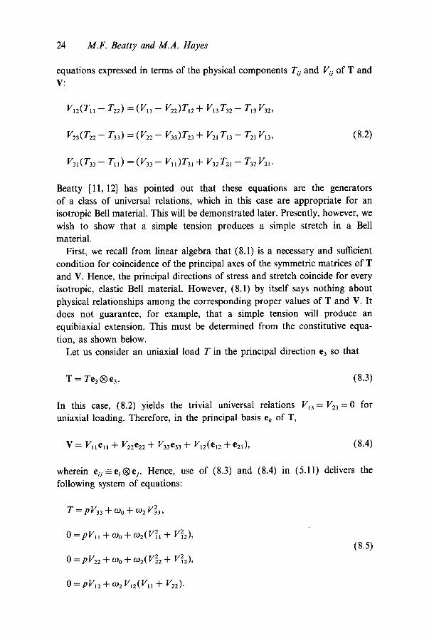
equations expressed in terms of the physical components T o. and V~ of T and V:
VI2(TII - T22 ) = (Vii -- V22)T12 "]- V13 T32 -- TI3 V32,
V23(T22 - T33 ) ~. (V22 - V33)T23 -Jff V21 T13 - T21 VI3, (8.2)
V31(T33- Tll ) ---~ ( V 3 3 - Vii)T31-[- V32 T 2 1 - T32 V21.
Beatty [11, 12] has pointed out that these equations are the generators of a class of universal relations, which in this case are appropriate for an isotropic Bell material. This will be demonstrated later. Presently, however, we wish to show that a simple tension produces a simple stretch in a Bell material.
First, we recall from linear algebra that (8.1) is a necessary and sufficient condition for coincidence of the principal axes of the symmetric matrices of T and V. Hence, the principal directions of stress and stretch coincide for every isotropic, elastic Bell material. However, (8.1) by itself says nothing about physical relationships among the corresponding proper values of T and V. It does not guarantee, for example, that a simple tension will produce an equibiaxial extension. This must be determined from the constitutive equa- tion, as shown below.
Let us consider an uniaxial load T in the principal direction e 3 so that
T = T e 3 (~) e 3. (8.3)
In this case, (8.2) yields the trivial universal relations Vi3 = V23 = 0 for uniaxial loading. Therefore, in the principal basis e, of T,
V = V~e~ + V~:e:~ + V33e33 + Vl~(el: ~ + e~), (8.4)
wherein e; j=e~®ej. Hence, use of (8.3) and (8.4) in (5.11) delivers the following system of equations:
T = pV33 + (.00 + 0 2 V~33,
0 ~-pVll dl- OJ 0 "~- o)2(V~l --[- V~2),
0 = p V : : + O9o + og:(V~: + V~:),
(8.5)
0 =pV12 -~- 0) 2 VI2(VI1 -]- V22 ).

An internally constrained material 25
Since e 3 is a common proper vector for both T and V, and because every direction in the 12-plane is a principal direction for T, we may always choose one such set to coincide with the principal axes nk for V. Then V12 = 0 and (8.5)2.3 yield the relation
(21 - 22)[-~0o + ~o:2122] = 0 (8.6)
in the principal frame where V = 2 k n k t~) nk, sum on k. Hence, if the inequal- ities (6.6) hold, (8.6) shows for the uniaxial loading (8.3) that
21 = 22, 23 = 2, say. (8.7)
It thus follows that every direction in the 12-plane is a proper direction for V; and therefore VI2 = 0 in all frames related by an orthogonal transformation R for which Re 3 = e 3 . Hence, in addition to sharing the same principal directions, T and ¥ have corresponding equal proper values provided the inequalities (6.6) hold. Thus, the inequalities (6.6) imply that an uniaxial load produces an equibiaxial deformation. Since the Bell constraint (2.4) provides the unique relation
21 =21(2) = ½ ( 3 - 2 ) for all 2 ~(0,3), (8.8)
the stretch (8.7), in the sense of Beatty and Stalnaker [8], is simple. Thus, an uniaxial load will produce a simple stretch in a homogeneous and isotropic, elastic Bell material, provided the inequalities (6.6) hold. Plainly, the result follows also from the stronger A-inequalities (6.11). Some additional proper- ties of a simple tension of a Bell material follow.
The maximum orthogonal shear component of V, hence also for Bell's strain E in (3.8), occurs on planes at 45 ° from the loading axis, as usual. Its magnitude, obtained from (8.7) and (8.8), is
(V3l)max:(E31)max=(~-~):~(2 - l) <~. (8.9)
We recall our earlier observation [8] that the Poisson function v(2) for a Bell constrained material in simple tension is constant: v(2)= Vo = ½ for all 2 ~ (0, 3). That is, the longitudinal extensional strain is exactly one half of the lateral contractive strain for all axial loads in a simple tension test of any Bell material whatever.

26 M.F. Beatty and M.A. Hayes
With the foregoing results in mind, we see that the system (8.5) may be rewritten as
T = p2 + 09 0 + 09 2 2 2,
p = __/~{1 (090 "]- 092212)" (8.10)
Substitution of (8.10)2 into (8.10)1 and use of (8.8) delivers the uniaxial stress-stretch relation for a homogeneous and isotropic, elastic Bell material:
[ 1 T(2) = 23-2(2 - 1) 032(2) 2(3 - 2)_] for 2 ~ (0, 3), (8.11)
wherein we have written coa(Hv, IIIv) = 03a(2) with
IIv = ~(1 + 2)(3 - 2), IIIv= ¼2(3 - 2) 2. (8.12)
Our earlier use of the terms "extension" and "contraction" was strictly intuitive. We did not actually establish that tension causes elongation while compression induces shortening of a Bell material. This is a separate issue which (8.1 1) can now render precise. Indeed, (8.1 1) shows clearly that tension (T > O) produces lengthening (2 > 1) and compression (T < O) produces shorten- ing (2 < 1) in an isotropic, elastic Bell material, i f and only if the inequalities (6.6) hold for the simple, equibiaxial deformation (8.7). The result (8.12)2 shows that in every equibiaxial deformation (8.7) of a Bell constrained material, the volume ratio IIIv = V/Vo decreases monotonically from its greatest value Vo in the undeformed state. This was illustrated earlier in Fig. 3.
9. Bell's stress tensor
In the previous section, it has been seen that physically consistent conclusions in simple tension lend support to the adoption of the inequalities (6.6) and (6.1 1). Parallel results may be readily established in terms of another symmet- ric stress tensor tt introduced by Bell [9], following a suggestion by Ericksen. We call ~ the Bell stress and given an alternative form of the constitutive equation in terms of it. This leads to introduction of other response functions and the inequalities (6.6) and (6.11) are recast in terms of these. We find that our inequalities for the principal Bell stress components are analogous to the Baker-Ericksen inequalities. For completeness, in §9.1 we also write the equilibrium equations and the traction vector in terms of a. Then in §9.2 we reconsider uniaxial loading, derive the corresponding uniaxial stress tr, and

An &ternally constrained material 27
compare our theoretical result for finite deformation of elastic materials with the experimental formula found by Bell [9] for plastic deformation of various metals. We show that our theoretical result includes as a special case Bell's parabolic law for the uniaxial loading test applied to nonlinearly elastic materials.
The Bell stress tensor is defined by
t~ = J V - ' T = RT~, (9.1)
in which TR is the engineering stress tensor, and J, V, and R are defined in (2.1). We recall that J = I I Iv . The reader will find that a is frame indifferent [6] if and only if T is also. In contrast, Bell [20] has shown that an incremental theory of plasticity that respects (2.4) and is based upon the Bell stress (9.1) is not objective. Bell's incremental theory invokes the further surprising experimental condition that R = 1, very nearly. One would not expect this to hold for the large twist of a tube, for example; but Bell's tests on the finite twist of thin-walled cylindrical tubes reveal that the rigid rotation part of the deformation is, in fact, minuscule. This torsion problem will be studied further in §15.
It is easy to see that the universal relation (8.1) yields the universal formula
V m T n = T " V " (9 .2 )
for all integers m and for all integers n ~> 0. In particular,
V- 1T = TV- 1, BT = TB, (9.3)
wherein we recall (2.2). Hence, (9.1) with (9.3)1 shows that t~r= ~, hence a is a symmetric tensor. The rule (9.3) also induces a universal relation in terms of o that follows from (9.1):
oV = Vtr. (9.4)
A relation similar to (9.2) holds also for o. Indeed, the rule (9.2) simply reflects the fact that for any tensor P the principal directions of P and pn are the same.
In terms of the Bell stress, use of (9.1) in (5.11) yields the following alternative form of the constitutive equation for an isotropic, elastic Bell material:
tr = q l + D I V + ~ _ I V -1, (9.5)

28 M.F. Beatty and M.A. Hayes
in which q = Jp is another undetermined constraint parameter and the re- sponse coefficients f~ and fl_ ~ are defined by
~ = IIivo92, fl_ ~ = IIIv~oo. (9.6)
It follows from (6.11) that the A-inequalities are equivalent to
f~ >0, f~_~ ~<0. (9.7)
It is evident from (5.11) and (9.5) that a principal direction Vk for V also is a principal vector for both T and t~. Indeed, (9.1) yields
~vk = J V - ~Tv k = Jte V - ~Vk = Jtk~,~ 1Vk ~ i~ k Vk (no sum). (9.8)
Hence, (6.3) reveals that the principal Bell stress components trk are the principal forces:
t~ tk =- T, =IIIv ~k = 2~2223 ~ (no sum). (9.9) t7 k
Thus, with (9.6) and (9.9) in (6.4), we learn that the OF-inequalities (6.5) are equivalent to the assertion that the greater principal stretch of a block of an isotropic, elastic Bell material occurs in the direction of the greater principal Bell stress; and distinct principal Bell stresses implies distinct principal stretches. Use of (9.6) shows that the inequalities (6.6), necessary and sufficient for this property, are equivalent to the conditions
1 ~-~1--~--~j.f~--I > 0 if,~i~2~, (9.10a)
12 ~ 1 - - ~ , . ~ _ ~ > 0 i f2 ;=2 j . (9.10b)
Hence, our inequalities (6.6) or (9.10) for the principal Bell stress components in an isotropic, elastic Bell material are the analog of the Baker-Ericksen inequalities for the principal Cauchy stress components in an unconstrained or incompressible, isotropic elastic solid.
9.1. The equilibrium equation and traction vector
Use of the equilibrium equation, without body force, and the uniform end loading condition in the uniaxial loading problem was implicit in our earlier

An &ternally constra&ed material 29
presentation for homogeneous and isotropic materials in terms of the Cauchy
stress. For the Bell stress, however, these familiar equations are quite different.
We find with (9.1) that the equation of motion and the stress vector when expressed in terms of the Bell stress require the following relations:
div T = J - l [ V div 6 + (grad V) • 6 - V6(V -1 • grad V)],
= j 1 V p [ ~ q k 3 I_ ~,-I'v-l~qlr --,k°sVrS~k - - (Tqk( V - 1)rs V~]ep (9.11)
t n = T n = J ~ V o n = o ( J - ~ V n ) , (9.12)
Div T~ = Div(aR) = (17~RJA),A e~, tx = T~N = aRN, (9.13)
where n and N are the unit exterior normal vectors to the boundary in x and
x0, respectively. The indexed relations respect familiar conventions of tensor analysis in which a comma denotes the usual covariant derivative. A relation similar to (9.11) in which the mutual positions of V and ~ are reversed also
may be obtained. When the body force is absent, the usual equilibrium equation div T = 0 yields from (9.11) and (9.13)1 the equilibrium equation for the Bell stress:
div o + V- l(grad V) • ~ - 6 (V- 1 o grad V) = 0, (9.14)
or in its component form
~r~,~ + (v-')f vj,~a ~ - (v-%vi~ ~ = o. (9.15)
Equation (9.12) shows that any null traction condition translates to ~, - -on = 0. It is evident that in general the equation of motion and traction condition usually will be more easily set in terms of the Cauchy stress tensor T.
9.2. Bell's empirical rule for uniaxial loading
In a pure homogeneous deformation, V is a constant tensor so (9.14) and (9.5) yield the equilibrium relation div o = grad q = 0 when the body force is absent. Hence, q must be constant.
For the uniaxial loading problem, for example, we have q = Jp, where p is given by (8.10)2. This aside, with the aid of (9.6) and (9.9), (8.11) yields the corresponding stress-stretch relation for the uniaxial Bell stress a in terms of

30 M.F. Beatty and M.A. Hayes
the engineering strain E = 2 - 1:
a = ~EI}(E) (9.16)
for - 1 < E < 2. Herein we recall (8.12) and write
2 f 2 , (9.17) fl(E) -- 1"}, ( 1 + E)(2 - E)"
Turning to experiments reported by Bell [1], we find that the result (9.16) for a general isotropic, elastic Bell material includes as a special case Bell's parabolic law for the uniaxial loading test:
a = 3~(sgn E)]E I L/2 (9.18)
for both tension E > 0 and compression E < 0. Herein the material constant y > 0. Thus, the response function in (9.16) for Bell's uniaxial loading test is identified explicitly by
f~(E) = ? [E[-~/2 (9.19)
for an isotropic, elastic Bell material. We shall return to this result and render it more precise in §17.1.
10. Principal directions and values of stress and stretch
In this section, we first review briefly the result that the principal directions for the Bell stress, the Cauchy stress, and the right Cauchy-Green stretch tensor coincide if and only if (8.1) and hence (9.4) hold. Then, by applica- tion of the inequalities (9.10), it will be shown that equal principal Bell stresses produce corresponding equal principal stretches in every isotropic, elastic Bell material. For the Cauchy stress, however, we are unable to establish completely the same rule when the Cauchy stress is an equibiaxial or hydrostatic, compressive stress. The analysis for both the Bell and Cauchy stresses is presented in turn. Afterwards, some specific results are described for an equibiaxial deformation and an example illustrates the disturbing conclusion that an equibiaxial deformation may be possible under an all- around compressive Cauchy stress.

An internally constrained material 31
10.1. Corresponding principal directions for ~, T, and V
It is clear from (5.11) and (9.5) that the principal directions of T and ~ coincide with those of V; and hence with each other. But the converse result is not equally evident. We know, however, that independently of material considerations, two symmetric tensors T and V have common principal directions if and only if they commute. Indeed, this may be seen briefly as follows.
Supposing that (8.1) holds, we let (2, v) be a proper pair for V, and write H ~ Tv. Then with (8.1), we obtain
VH = TVv = 2(Tv) = 2H.
Hence, H also is a proper vector parallel to v, that is, H = Tv = tv for some scalar t. Conversely, if v is a common proper vector for T and V, then
TVv = 2Tv = 2tv = t V v = VTv.
That is, ( T V - VT)v = 0. Hence, if T and V are symmetric, (8.1) follows in view of the linear independence of their three proper vectors. Of course, the same thing holds for ~ in (9.4). Thus, regardless of the nature of the material response functions and the undetermined constraint reaction parameter, the principal directions for ~, T, and V coincide. However, on this basis alone, nothing more may be said about the physical relationships among the respective proper values of ~ and V, T and V, or T and ~.
We recall, for example, that Batra [13] has proved further that for a compressible or incompressible, isotropic material, T and B also will have corresponding equal proper values provided the empirical inequalities (6.7) hold, or, more weakly, if the Baker-Ericksen inequalities hold [6]. Our previous result for the special simple tension problem certainly suggests that a parallel theorem ought to hold for an isotropic Bell material, but a somewhat different approach is needed to prove this.
10.2. Corresponding pr&cipal values of t~ and V
To establish the result that equal proper values of ~ implies corresponding equal principal values of V, we first note that (9.4) yields equations of the form (8.2) in terms of a,.j. Thus, in the principal reference system ek for t~, the universal relation (9.4) yields
(~1--o2)V12 =0, (~2--ff3)V23=0, (03--~1)V31=0. (10.1)

32 M.F. Beatty and M.A. Hayes
Notice that when the principal Bell stresses o k are distinct, (10.1) shows that the principal directions of V coincide with those of t~, regardless of the form of the response functions, as proved above. Suppose, however, that two principal values of t~ are equal, say, a~ = a 2 = r ~a3 . Then (10.1) yields
V23 = V3~ = 0. Hence, e 3 is a mutual principal vector for both ~ and V, and (9.5) yields the system of equations
tr3 = q + ~ V33 + f~_ ~ V~ 1 , (10.2a)
V22 Z = q q " ~ ' ~ i V l l + f ~ - I C ' (10.2b)
V11 ~ = q + D ~ V ~ 2 + ~ - ~ C ' (10.2c)
( 1 ) 0 = V~2 f~ - ~ f~_ ~ , (10.2d)
wherein C = VI~ V22 - - Vi22 > 0 for positive, symmetric V. We notice that if the A-inequalities (9.7) hold, the last of (10.2) yields
V12 = 0. This aside, we see more generally that because e3 is a mutual proper vector for ~ and V and every direction in the 12-plane is a principal direction
for t~, without loss of generality, we may select a reference set that coincides
with the principal directions for V. Then V12 = 0 and it follows from (10.2)2,3 that in the principal basis for V,
(,~1- ,~,2)(~r~l- ~ 2 ~"~_ 1 ) ~--- 0. (10.3)
Thus, /f the (weaker) inequalities (9.10) hold, equal biaxial principal Bell stresses a~ = tr 2 produce corresponding equal biaxial principal stretches ).~ = 22 in an isotropic, elastic Bell material. Notice that it then follows again that every direction in the 12-plane is a principal vector for V; and hence V~2 = 0 in all reference frames related by a rotation around e3. In this case, the internal constraint (3.1) yields the relations (8.8) and (8.12) valid for all equibiaxial deformations (8.7).
Finally, let us suppose that all three principal Bell stresses are the same: trk= Z, say. Then every direction is a principal direction for a, and hence a reference basis that coincides with the principal set for V may be chosen so
that (9.5) yields
"t" = q - + - ~ ' ~ l ~ . k - [ - ~ " ~ _ l J , ~ -1 , k = 1 , 2 , 3 . (10.4)

An internally constrained material 33
Forming differences among the three pairs of equations in (10.4), we obtain
(,~k -- /],j) If~l -- ~j--~k f~_ 11 = O, k :/:j = 1, 2, 3. (10.5)
Clearly, if the inequalities (9.10) hold, all 2k = )~, say; but the constraint (3.1) then shows that 2 = 1. Hence, as shown differently in (5.13), no amount of hydrostatic Bell stress can induce a uniform dilatation of an isotropic, elastic Bell material from its natural, undeformed state.
Thus, ~f the inequalities (9.10), or equivalently (6.6), hold for an isotropic,
elastic Bell material, then equal biaxial principal Bell stresses will produce corresponding equal principal stretches for which (8.8)must hold. Moreover, an
all-around Bell stress will produce no deformation whatever f rom the natural
state o f any isotropic, elastic Bell material.
10.3. Corresponding pr•cipal values o f T and V
Although distinct ak imply distinct 2k, and conversely, we notice that the relations (9.9) do not imply that the principal Cauchy stresses tk need be distinct. The product at21 = I I I v f i , for example, may be the same as a222 = I l lv t2 , even though at # a2 and 2j ¢ 22. Thus, though the principal axes of T, V, and tr coincide, equal principal values of T may not imply corresponding equal principal values for V nor ~, unless of course the equal principal values for T are zero. The latter fact was proved earlier for the uniaxial loading and stress-free problems under the condition that our in- equalities (6.6) hold. Thus, at this point, with our results on a and V, for the equibiaxial case we know only that in a mutual principal reference system
ai = e~ ~ 2i = 2j =:" ti = O' (lO.6a)
ti : ty : O =~ ~,i : )~ j. (lO.6b)
For the all-around stress problem, we have
a k = r c ~ 2 k = l = : ' t k = z , r # 0 . (I0.6C)
For the stress-free state, we know that
a~ = 0¢~ tk = 0 ~ 2 k = 1. (lO.6d)
To complete the argument, the converse in (10.6b) and the last implication in (10.6c) must be strengthened. However, we have only a partial proof, as follows.

34 M.F. Beatty and M.A. Hayes
10.3.1. The equibiaxial Cauchy stress problem First, we consider the equibiaxial stress problem. Let us suppose that ti = tj = z ~> 0. Then, in a mutual principal reference system, (6.2) shows that
(2,-- 2j)Iz + 2i2j(c02- 2~. co0) ] =0 . (10.7)
Therefore, if our inequalities (6.6) hold, it follows that 2i = 2j. We thus conclude the partial result
ti = t j >/ O => ).i = ). j , (10.8)
provided the inequalities (6.6) hold. We find, however, no contradiction if z < 0 and satisfies (10.7). This implies that without further restrictions the constitutive equation (5.11) may admit the possibility of a plane shear deformation supported only by normal tractions, at least two of which are equal compressive stresses.
In view of our previous success in the proof of (10.6a)l, it is natural to pursue a parallel result based on (8.2). Thus, suppose that tl = t2 = z, say. Then (8.2) shows that V13 = V23 ~- 0, and hence e 3 is a mutual principal vector for both T and V, and (5.11) yields
t 1 = r =pVll q- 090 + c%(V121 + V22), (10.9a)
t 2 = "C = p V 2 2 q- (.% -b (.02(V222 -[- V22) , (lO.9b)
t 3 = p V33 -~- (.D O + (-0 2 V23, (10.9c)
0 = V~2[p + 092(V1~ + V22)]. (lO.9d)
Thus, upon eliminating p between pairs of (10.9a), (10.9b), and (10.9d), we find
det V~ ( V22 - - V11 ) "c - - (2) 0 -4- 0) 2 V33 ] = 0, ( 1 0 . 1 0 a )
z
det V~ V12 r - COo + co2-~33 ) = 0. (10.10b)
Consequently, if z ~> 0 and the inequalities (6.6) hold, it follows that in the mutual principal reference system of T and V where V~2=0, we have V~ = V22. That is, 21 = ).2 and hence V12 = 0 in every reference system
An internally constrained material 35
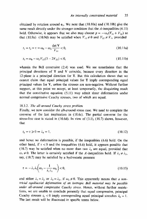
obtained by rotation around e 3. We note that (10.10a) and (10.10b) give the same result directly under the stronger condition that the A-inequalities (6.11) hold. Otherwise, it appears that we also may choose p = -o92(V~1 + V22) so that (10.9a)-(10.9d) may be satisfied when V~ :~ 0 and V~ g: V~ provided
det V tl = t 2 = z = ~Oo- ~o2 ~ < 0, (10.11a)
v 3 3
t3 = Ogo - ~O2 V33( 3 - 2V33 ) <0, ( 10.1 lb)
wherein the Bell constraint (2.4) was used. We see nonetheless that the principal directions of T and V coincide, because every direction in the 12-plane is a principal direction for T. But this calculation shows that we cannot claim that equal principal values for T imply corresponding equal principal values for V, unless the stresses are non-negative. Without further support, at this point we accept, at least temporarily, the disquieting result that the constitutive equation (5.11) may admit shear deformation under normal compressive Cauchy stresses, two of which are equal.
10.3.2. The all-around Cauchy stress problem
Finally, we now consider the all-around stress case. We need to complete the converse of the last implication in (10.6c). The partial converse for the stress-free case is stated in (10.6d). In view of (3.1), (10.7) shows, however, that
tk=z/>0=~2g----1 , (10.12)
and hence no deformation is possible, if the inequalities (6.6) hold. On the other hand, if ~ < 0 and the inequalities (6.6) hold, it appears possible that (10.7) may be satisfied when no more than two 2k are equal, provided that tn 2 # 0. The latter is certainly satisfied if the A-inequalities hold. If 21 ~ 23, say, (10.7) may be satisfied by a hydrostatic pressure
-r=-2,2~(~- 2-~2~ ~o)<0, (10.13)
and either 21 = 22 o r 23 = 22, if ~o2 # 0. This apparently means that a non-
trivial equibiaxial deformation o f an isotropic Bell material may be possible
under all-around compressive Cauchy stress. Hence, without further restric- tions, we are unable to conclude presently that equal compressive, principal Cauchy stresses tk < 0 imply corresponding equal principal stretches 2k = 1. The last result will be illustrated in specific terms below.

36 M.F. Beatty and M.A. Hayes
10.3.3. Remarks on equibiaxial deformation and the Cauchy stress Let us consider an equibiaxial, homogeneous deformation xk = 2kXk (no sum) for which 21 = 22 ~ 23. Then (2.1) and (2.2) provide
2 2 . V=2~e~t +21e2:2+23e33 , B=212ell +21eT.~+23e33 , (10.14)
and (5.11) yields
T l l = T22 = p A 1 -~- (D O -~- (.02212, (10.15)
T33 =PJ.3 + (Do + 0)2232. (10.16)
Of course, p is arbitrary and may be chosen to satisfy various conditions. If p is chosen so that Tll = T22 = 0, we get our previous result (8.10) for uniaxial loading; but if we select p so that T33 = 0, we have the all-around plane stress solution
P = 2, (~],l- 23)[(D2 - ~ (Do], (10.17)
in which P = T~ = T22. Suppose that (6.6) holds. Then P > 0 is an all-around plane tension when 21 > 23; otherwise, P < 0 is a pressure when 2~ < 23. By introduction of the Bell constraint (3.1) into (10.17), we have the required all-around plane stress
E 1 1 3 P =32~(2~- 1) (D2--2~(3_2,,~l)(D o , 0<2~ <~. (10.18)
Thus, P > 0 when 1 < 2 t < I; and P < 0 when 0 < 2~ < 1, consistent with the physical nature of the problem. Hence, an equibiaxial deformation supported by an all-around plane Cauchy stress is physically possible in an isotropic, elastic Bell material. However, (10.8) shows that we have been unable to establish the converse result for a compressive Cauchy stress. The reader will see that the equibiaxial case 2~ = 22 corresponds in Figs. 2 and 6 to the line AOD. It should be noted that the extensional case OA requires 23 > 1, hence P < 0 in our example. Similarly, the compressional case OD means that 23< 1 , P > 0 .
Returning to our question concerning an equibiaxial deformation supported by an all-around Cauchy stress ~ = Tll = Tz2 = T33, we need to determine p in (10.16) so that
Tll - T33 = (2~ -- 23)[p + (D2(2 + 23) ] = 0 (10.19)

An internally constrained material 37
while 2~ ~ 2 3. We thus take
P = -o92(21 + '~3)" (10.20)
When this is substituted into (10.15), we indeed derive the required all-around stress
~=-2~3(~o2 - ~,~3 o~0 ) (10.21)
This relation coincides with (10.13); and, as before, if (6.6) holds, (10.21) shows that the stress must be compressive, z < 0. It thus appears that an all-around pressure may support a nontrivial deformation in which only two of the corresponding principal stretches are equal. If 21 = 22 < 1, for example, the constraint (3.1) requires 23 = 3 -221 > 1. Therefore, an isotropic Bell material, without further restriction on its response, may expand in at least one direction under a uniform hydrostatic pressure, an effect contrary to our physical intuition. By (9.9), however, we find the physically consistent and corresponding equal compressive Bell stress components for the equibiaxial deformation:
al = o2 = 2123z, a3 = 2~z. (10.22)
11. Universal relations
The importance of the universal relations (8.1) and (9.4) has been illustrated in the previous analysis. Specific universal relations generated by (8.1) or (9.3) for T and by (9.4) for a are equivalent; and (8.2) shows that no more than three such relations may be obtained. These reduce to a single equation when one coordinate direction is a principal direction. In particular, when e3, say, is a principal vector for V so that V has the representation (8.4) in an otherwise arbitrary physical basis ek, both T and ~ have similar representa- tions in e~. Consequently, as demonstrated by (8.2), the general rules (8.1), (9.3)2, and (9.4) yield the single universal relation
0"II--0"22 T,, - T22 B,I - B22 Vtl - V22 D
O"12 TI2 B12 Vl2 (11.1)
This rule derives solely from the algebraic structure of the aforementioned equations, and thus holds independently of the constitutive equation and of the equations of balance. Indeed, with proper latitude in the identification of

38 M.F. Beatty and M.A. Hayes
B, a general rule of the type (11.1) holds for both solids and fluids for which a commutative rule (8.1) relating the stress to the deformation or the rate of deformation may be assured. It thus holds for every compressible and incompressible, isotropic elastic solid; it holds for every isotropic fluid; and it holds for an isotropic Bell constrained material. It holds also for the extra stress on any isotropic material with a workless kinematical constraint [12]. Moreover, it holds for both static and dynamic motions, because the rules themselves have nothing to do with the equations of motion. Of course, in order that a given deformation or rate of deformation may in fact yield a solution for which the universal rule may then stand, it is necessary eventually that the equations of balance be satisfied.
Further, it is well-known that for a symmetric tensor having the representa- tion (8.4), the orthogonal principal directions in the 12-plane are determined by the elementary formula
2V12 2Blz tan 20 - V,, - V22 - B,, - B22" (11.2)
As usual, 0 • [0, ~/2] is the angular placement of one of the plane principal directions of V and B from the assigned coordinate direction e~. It is also well-known that the planes of maximum shear are oriented at + 45 ° from the principal directions at 0, that is, at angles ~ = 0 ___ rt/4 from e~.
The importance of these kinds of universal rules has been discussed recently by Beatty [11, 12, 14]. Their further application will be demonstrated in some work that follows; but first we shall describe a straightforward method for the determination of the left stretch tensor.
12. Determination of V for essentially plane problems
In applications of the theory, it is necessary that we determine V = B 1/2 for various kinds of deformations, usually a tedious calculation. However, this task is much simplified when V has the typical representation (8.4) in an orthogonal physical basis etc. That is, when
V = V 2 --I- ,~3e33, (12.1)
in which Vz is the two dimensional tensor
V2 -= Vl,ell + V22e22 + V12(e12 + e21). (12.2)

An internally constrained material 39
In addition, we have
V -1 : V~ -1 + ,~1e33,
wherein
(12.3)
1 V 2 ' - [V2ze,, + Vl~e~2- V12(e12 +e21)]. (12.4)
det V2
In similar notation, we obtain from (2.2) and (12.1)
B=B~+2~e33 withB2--V22. (12.5)
Our objective is to determine V2 in terms of B~ rather B~/2 for the class of two dimensional problems with normal stretch 23 characterized by (12.1). These are called essentially plane problems. Afterwards, some additional principal stretch relations will be described.
Following Ting [3], we apply the Cayley-Hamilton theorem to V2 to get
B2 = V2 ~ = (tr V2)V 2 - - (det V2) 12, (12.6)
in which
t rV2= VII "q- V22 , detV2 = Vi i V22 - V122, 12 = e l l q - e 2 2 , (12.7)
both invariants being positive. With the aid of the determinant of (12.5)2 and the trace of (12.6), (12.6) itself can be solved to obtain the desired useful formula
Bz + (det B2) 1/212 = (12.8)
V2 x/tr B 2 + 2(det B~) ~/~"
In addition, we find from (12.1) that the Bell constraint (2.4) may be written as
t r V = A +23=3 , (12.9)
in which
A = tr V 2 = x/tr B 2 + 2(det B2) ~/2. (12.10)

40 M.F. Beatty and M.A. Hayes
The formulas (12.8) and (12.10) are expressed entirely in terms of the easily computed two dimensional part orb in (12.5). Consequently, V itself may be more readily calculated by use of (12.8) in (12.1). A formula of the type (12.8) for the stretch tensor U = C m, its extension to the general three dimensional case, and some other relations for isotropic tensors are described by Ting [3]. Similar two and three dimensional formulas have been presented recently by Stickforth [ 15].
Finally, it is useful to note that in terms of the plane principal stretches 2k, k = l , 2 ,
d e t 172 = d e t V 2 = (det B 2 ) 1/2 ~_ 2 1 2 2 ,
t rV2=21+J.2, trBz=212+22. (12.11)
The first of these invariants, in evident notation, follows from (2.1) which reveals that 172 = V2R2 for R = R2 + e33. Hence, we find from (12.8), or directly from (12.6), the alternate formula
B 2 q- (det 172)12 B 2 d- 212212 V2 = - (12.12)
x/tr B2 + 2(det F2) 21 JI- 2 2
The characteristic equation for V2 may be simply written as
det(V2 - - 2 1 2 ) = 22 - - A 2 + d e t F 2 = 0 . (12.13)
Hence, the plane principal stretches are determined by
2 1 = 1 ( A + B ) , 2 2 = l ( A - B ) , (12.14)
wherein, with the use of (12.10), we identify
A = ,~,1 + 22 = ~/tr B 2 + 2 det F 2 ,
B = 21 - 22 = N / A 2 - 4 det F 2 .
(12.15)
The Bell constraint (12.9) has, of course, the familiar form (3.1) and thus restricts the third principal stretch so that
2 3 = 3 - A = 3 - ( 2 1 + 2 2 ) . (12.16)
The relations presented above are valid for all essentially plane problems. We are now prepared to examine some examples.

An internally constrained material 41
13. Pure shear and Bell's experiment
Here we study the pure shear of a materially uniform rectangular block. For this deformation, E2 = 0 and E~ + E3 = 0. We determine the corresponding Bell stress components for an isotropic, elastic material and compare their ratio with the experimental result reported by Bell [1] for finite strain of
metals. It is found that the results are compatible if and only if the response
function f~_ 1 vanishes in every pure shear. The A-inequalities (9.7) admit this possibility. If this is so, then the theoretical result includes as a particular case Bell's parabolic law for pure shear [1]. Of course, our result is restricted to this
special class of isotropic, elastic Bell materials. Let us consider a homogeneous deformation of a materially uniform,
rectangular block whose plane ends X = ___ a are subjected to uniform tensile or compressive loading while its faces Y = + b are restrained, and its surfaces Z = + c are traction free. The deformation is described by
x=2~X, y = Y , z = 2 3 Z , E 2 = 2 2 - 1 = 0 (13.1)
in a Cartesian frame ~p = {O;ek}. In this case, V is readily determined; we
have
V = F = 2 ~ e ~ -[- e22 --I- ~3e33 , (13.2)
and
V - 1 = A l - l e l l -[-e:~ z q- ~,~-1e33. (13.3)
The Bell constraint (3.1), or equivalently (3.10), requires
2 1 + 2 3 = 2 , or E l + E 3 = 0 . (13.4)
The principal invariants are given by
IIv = 2+2~).3 = 3 - - E l ~, IIIv=2~23 = 1 -E2~, (13.5)
in which (13.4) has been used.
To characterize the deformation (13.1) under the constraint (13.4) as a pure shear, we consider the Bell strain (3.8) in a reference frame ~p'= {O;e~,} rotated through 45 ° about the mutual axis e~ = e2. It turns out that its only nonzero component is
t / I E l 3 = E31 = ~("~3 - - 2 1 ) = 1 - 2~ = -E~ = E 3. (13.6)

42 M.F. Beatty and M.A. Hayes
Hence, the deformation (13.1) under the constraint (13.4) indeed characterizes kinematically the pure shear studied in experiments by Bell [1]. The Bell stress components that support this deformation are readily determined.
Substitution of (13.2) and (13.3) into (9.5) yields the principal Bell stress components
a l = q +21f~1+2i -lf~ l, (13.7)
0"2 = q + ~ 1 + f~ 1, (13.8)
0"3=q ~- ~3~1 q- 2~-1~_1 . (13.9)
The equilibrium equation (9.14) becomes d i v a = 0 ; and this is satisfied without body force provided q is constant. The null traction condition t 3 = 0 on the ends z = ___ c23, in accordance with (9.9), is equivalent to 0"3 = 0. Thus, by (13.9), the constant q may be chosen as
q = --/~.3~'~1 - - / ~ - 1 ~ ' ~ _ 1 . (13.10)
We use this in (13.7) and (13.8) and recall (13.4)1 to derive
( l ) , ( 1 3 . 1 1 )
0 " 2 = ( 1 - ) ~ ) ( n l - ~ - 3 n _ l ) . (13.12)
In view of (13.4), 0 < 2k < 2. The response functions f~r in these equations depend on the invariants in (13.5).
It remains to consider the tractions on the uniformly loaded and restrained surfaces. With the aid of (13.4)1 and our inequalities (9.10), we first note from (13.11) and (13.12) that
0-1 -- 0"2 0"1 -- 0"2 ~ 7-l f n_l>O, (13.13)
If the planes X = _ a are subjected to uniform tensile loading 0-~ > 0, it follows from (13.11), (13.13), and the constraint (13.4)1 that 21 > 1 >23. Therefore, our inequalities (9.10) applied to (13.12) show that a2 on the restrained surface also is a tensile load, and (13.13) indicates that 0-~ > 0-2- Otherwise, 2~ < 1 < 23 and both 0-~ and 0-2 are compressive loads such that 0-~ < 0-2 < 0. It is clear also from (13.11) and (13.12) that the stress vanishes on

An internally constrained material 43
one face if and only if it vanishes on the other. Hence the implications of our
A-inequalities are consistent with the physical nature of the problem. In either
case, Jail > [¢r21 and we may write their ratio
tr 2 1 ~'~1 - - • 3 l~'~ 1 < 1. (13.14)
O" 1 - - 2 ~ 1 - - 2 1 1 ~ 1 ~ ' ~ _ _ 1
Herein we recall (13.5) and note that for the pure shear
f / r(IIv, I I I v )= f21-(3-e~ 2, 1 - - e~ 2) -- ~r(E~2), F = 1, - 1 . (13.15)
13.1. Bell's empirical relation for pure shear
Bell [1] has described a pure shear experiment controlled so that ~r2/tr I = 1/2
and the constraint E3 = - E l in (13.4)2 is respected. In other tests he has demonstrated that the material response of his specimens was isotropic. We see from (13.14) that this empirical result is possible in our isotropic, elastic
Bell material if and only if f~_ 1 = 0 in the pure shear test. Moreover, our
A-inequalities are consistent with this empirical condition. In this case, (13.11), (13.12), and (13.15) reveal that
el = 2a2 = 2E1 fil (E~) = 2E 1 ~( IEI I), (13.16)
where - 1 < El = 21 - 1 < 1 and we have put f~(IE1 l) -= fil(E~). This theoreti- cal result for an isotropic, elastic material is consistent with and includes as a particular case Bell's parabolic law for the pure shear test:
Ol = 2~(sgn E 1 )lE1 I 1/2 (13.17)
for both tension E 1 > 0, the present case, and compression El < 0. Thus, in this instance the response function in (13.16) is explicitly identified by
n(IE1 I) -- ~ IE1 l- 1/2, (13.18)
in which the material constant • > 0. For the pure shear data shown in [1],
we find that IE11 < O.lS. Although (13.18) is similar to the formula (9.19) for uniaxial loading, it should be noted that the response functions are different.
We have seen that the experimental data obtained in pure shear appear to support our A-inequalities (9.7). We emphasize, however, that the result f~ l = 0 in every pure shear need not hold in all deformations of a Bell material. Nevertheless, the fact that it does vanish in this test provides support

44 M.F. Beatty and M.A. Hayes
for study of the class of Bell materials for which f~_~ = 0 in (9.5):
o = q l + ~1 v. (13.19)
This rule is similar to the constitutive equation for the well-known and analytically useful incompressible neo-Hookean material described by T = - p l + fl~B, where fll is a material constant. It is seen from (9.6)2 and (5.11) that the equivalent equation in terms of the Cauchy stress with the condition COo = 0 is given by
T = pV + 0)2 v2. (13.20)
14. Simple shear superimposed on a triaxial stretch
A simple shear, of course, is different from a pure shear. In fact, we have seen that a simple shear is impossible in a Bell constrained material. On the other hand, we saw also that a generalized shear with normal stretch is kinemati- cally admissible. The generalized shear (3.3), however, is a special case of a generalized shear with stretch first introduced by Wineman and Gandhi [4] and studied further by Rajagopal and Wineman [5]. The deformation is a simple shear of amount K superimposed on a homogeneous triaxial deforma- tion with stretches /~k and defined by
x ~ - l g l ~ ¥ - ~ K ~ 2 Y , y = # ~ Y , z = # 3 Z . (14.1)
As usual, (x, y, z) is the image in x of a material point whose place in Xo was (X, Y, Z) in a common rectangular Cartesian frame ~0 = {O; ek}. The shear occurs in the 12-plane, and the angle of shear is F = t an- l K.
The component matrices of F and B defined in (2.1) and (2.2) are thus given by
F =/qel~ + ~2e22 + K/,t2e12 + ]~3e33, (14.2)
B ---- ( ~ + K2/~)ell + #zZe2z + K#~(e12 + ez~) +/,t 32e33 . (14.3)
14.1. The universal relation for shear with triaxial stretch
The single universal relation provided by (11.1) for the shear/stretch problem follows immediately from (14.3). We find
T l ~ - T22 a ~ - a 2 2 ~t 2 - 1 + K 2 ~q = - - = with # --- (14.4)
T12 a12 K #2"

An internally constrained material 45
This is precisely the universal relation discovered by Wineman and Gandhi [4] by altogether different means. Although they considered only incompressible, isotropic elastic solids, in fact, the universal rule (14.4) applies to compressible solids as well. Moreover, we see that Rivlin's universal relation for simple shear [ 16], namely,
T11 - T22 - - - K , ( 1 4 . 5 )
T12
holds also for a simple shear superimposed on a homogeneous triaxial stretch, if and only if fi = 1, that is, for any equibiaxial deformation #1 =/~2 with arbitrary normal stretch/~3, as observed previously in [4]. It thus holds for a simple shear with normal stretch when #1 =/~2 = 1, kt 3 = :t in (3.4). In addi- tion, it holds for a simple shear superimposed on an isotropic stretch for which all #k = it. In the case of a Bell material, of course, the constraint (2.4) also must be satisfied. We shall return to this momentarily; but first we shall examine the kinematical structure of the deformation (14.1).
14.2. Kinematics of deformation in the shear/stretch problem
The left stretch tensor and its principal values, directions, and invariants, and the rotation tensor for the deformation (14.1) will now be determined. The straightforward application of (12.1), (12.3), (12.11), and (12.12)1 to (14.2) and (14.3) yields the stretch tensor and its inverse (12.3). Thus,
1 V : ~ {[#, (:q -I- #e) -+- K~/~]e~ -I-/~e(bq + #~)e=
q- K#~fe12 q- e~)} q-/.t3e33 ,
I V-1 = {#2(/~1 +/~2)ell + [/~1 (#1 +/~2) + K2/~]e=
A#1 ~
- K~(e~z + e~)} + ~;~e33.
We notice in this case that
det F2 = det V: = ~lg2 = 2~22;
and equations (12.15) yield
A = 2~ + 2z = ~ ( ~ + ~2) 2 + K~.~,
(14.6)
(14.7)
(14.8)
(14.9a)

46 M.F. Beatty and M.A. Hayes
B = 21 - 22 = ~//A 2 - 4/~,/~2 = ~ / ( # , - / ~ 2 ) 2 + K2/~2~, (14.9b)
wherein, without loss, we have ordered 21 ~> 22. Hence, equations (14.9) determine the principal stretches (12.14). It may be seen that the squared stretches agree with those given by Wineman and Gandhi [4].
The formula (11.2) locates the vl principal direction for 21 in the plane of shear at the placement 0 from the el coordinate direction. Hence, with (14.6), we have
1 , ~ n - l [ - 2K#~ 1 0 = ~ i : t | , 2 , - T ~ /t'2, 2 • (14.10) LII~I--~'2 TI~- /~2
The direction for 22 is defined by v2 = v3 × vl, with v 3 ~ e 3. The maximum orthogonal shear component of V in the plane of shear is
given by (14.9b). We get
B ( Vl2)max -- ~ -- 21-~(]~1 -- #2) 2 -F K2#~, (14.11)
which is independent of/~3. We recall, however, that this need not be the greatest orthogonal shear, as demonstrated earlier in §3.3 in a related problem of generalized shear with normal stretch.
The rigid rotation tensor in the polar decomposition (2.1) is given by R = V-~F, and hence use of (14.2) and (14.7) yields
g~2 R - kq + #2 (e~ + e22) + (e12- e21) + (14.12) A ~ - e33'
where A is given in (14.9a). Therefore, the axis of rotation is e3, of course, and the angle of rotation ~ is given by
K~2 (14.13) tan 4) = #~ + #2"
The Bell constraint (12.16), by (14.9a) becomes
23 = #3 = 3 - A = 3 - ~//(#l + #2) 2 + K2#22. (14.14)
It is also relevant to recall for the Bell material the volume rule (3.2)3. Equation (14.2) gives easily
V - - = det F = det V = #1•2#3 = ~12223 ~ 1, (14.15) Vo

An internally constrained material 47
the equality holding only in the undeformed state. Finally, we recall with the aid of (3.1) that IIv = 2122 + 2 3 ( 3 - 23) and use (14.8), (14.14)1, and (14.15), to obtain the principal invariants in terms of the coordinate stretches Pk:
IIv = #~/~2 + #3( 3 - g3), IIIv =/~,/a2#3. (14.16)
14.2.1. The equibiaxial case I~1 = #2 = V, ~3 = ].l Several special cases are possible. One example is a simple shear superimposed on a normal extension for which/~l =/~2 -- v in the plane of shear and #3 ~- ~ normal to it. The principal stretches provided by equations (14.9) are then given by
; ; 21 =V ~"~- 1 " ~ - ~ , /~2=V---~ '~- l ' - ~ - ~ - , 23=]./, (14.17)
and
2122 = V 2, (14.18)
The angle of rigid rotation (14.13) and the maximum shear (14.11) in the plane of shear are given by
2 tan q~ = K = tan F, (Vi2)max = v tan ~b. (14.19)
The angular placement 0 of the proper vector Vl for 21 is provided by (14.10). With 2~b = (r~/2)- 20, we see more readily that tan 2~b = K/2 = tan ~b, and hence
0 = ~ _ ~ t a n _ l K rc q~ -~ 4 2"
Independently of the equibiaxial, pure homogeneous deformation, the formulas (14.19)1 and (14.20) relate the rotation angle q~, the principal angle 0, and the angle of shear F by the same rules known for a simple shear [17, §45]. Moreover, we see that (14.17) and (14.19)2 are proportional to the corresponding values for a simple shear to which they reduce when v =/~ = 1.
So far, the Bell constraint (14.14) has not been used. This yields the kinematical condition
K2 / ~ = 3 - - 2 v l + - ~ - = 3 - 2 v s e c q ~ (14.21)

48 M.F. Beatty and M.A . Hayes
relating the equibiaxial, pure homogeneous strain to the amount of shear and to the rigid rotation angle in (14.19)~. The volume constraint (14.15) essential for all Bell constrained materials further requires
/~v 2 < 1. (14.22)
14.2.2. The special case v = 1
In a simple shear for which v =/~ = 1, (14.21) holds only when K = 0 and then (14.22) can not be satisfied. Therefore, as shown before, a simple shear is impossible in any Bell constrained material.
On the other hand, when only v = 1, the constraints admit a simple shear with transverse stretch/t normal to the plane of shear, but only for a contraction # < 1. The deformation is determined completely by the kinematical constraint (14.21). The volume reduction/~ as a function of the amount of shear described by (14.21) is shown graphically in Fig. 7, and the corresponding deformation trajectory in the invariant plane is shown in Fig. 4.
Our present example is the special case (3.4) of the generalized shear with normal stretch described in (3.3). Therefore, the transition points of maximum orthogonal shear for V are given by (3.7a) and (3.7b) in which # is now
0 >
I!
0
o=
0
0 _1
¢:~
E
0 >
i.25 Natural State
0.75
o. o_
_ .V/.~/ 0.25
I I o - 3 -2 - I
. ~ ~ =3-JK2+4 =1
-
13 ,½1 Max. Sh Transition Point ~ ~
I 0 I 2
Amount of Shear, K
~
5
Fig. 7. Volume reduction (or lateral contraction) in a simple shear with normal stretch as a function of the amount of shear K. See also Fig. 4.

An internally constrained material 49
explicitly related to the amount of shear K by (14.21). For illustration, we assume K > 0. In this case, we find that (Vt2)max = K/2, in agreement with (14.19), is the greatest orthogonal shear for ½ </~ < 1 (or ~ > K > 0), whereas (V~3)max=¼[K-6+(K2+4) ~/2] is the greatest orthogonal shear for
x/~ ~ (at K = 232) where 0 < # < 3~ (or > K > -32), the transition occurring at/~ = 5 the two orthogonal shears are equal to ¼.
14.2.3. The special case # = v < 1 We see from (14.21) and (14.22) that a simple shear superimposed on an all-around stretch also is kinematically possible, but only for all-around contraction. Notice that neither deformation, as in the previous problem of shear with normal stretch, is separately possible, the shear and contraction must vary together consistent with the Bell constraint. Hence, the deforma- tion in this case is determined entirely by (14.21).
14.2.4. Other cases It is of interest to note that other cases are kinematically possible. These include (i) a simple shear superimposed on an extension #1 =/~ in the direction of shear with #2=/~3=v normal to it, (ii) a simple shear with extension ~t2 =/~ normal to the shearing planes with equibiaxial lateral stretch /h = #3 = v, and (iii) a generalized shear with normal stretch defined by (3.3). An important application of case (ii) will be presented in §15.
14.3. The Bell stress in the shear/stretch problem
A kinematically admissible deformation that can be produced in a material by application of suitable surface tractions alone is called a controllable deformation. A controllable deformation that can be effected in every homo- geneous, isotropic Bell material is called a universal deformation. It is evident from (9.5) and (9.14) that any time independent homogeneous deformation that satisfies the Bell constraint (2.4) is a controllable, equilibrium deforma- tion for every homogeneous, isotropic Bell material for which the constraint parameter q is an arbitrary constant. Hence, homogeneous deformations that satisfy (2.4) are universal deformations. The simple shear with normal stretch defined by (14.1) is an example for which we shall now determine the Bell stress relations.
Use of (14.6) and (14.7) in (9.5) yields the Bell stress components for the shear/stretch problem. We have
ol O'll = q + ~ - [ l - / l ( l - / l ' - ~ / 2 ) - [ - K 2 # 2 2 ] ' - ~ (]./1+/,/2) , (14.23a)

50 M.F. Beatty and M.A. Hayes
~"~1 ~"~-- 1 a22 = q + -~- #~(#, + #2) + ~ []'~1 (~1 "1- ~2) "~ K2/~221, (14.23b)
0"33 = q + f ~ l # 3 "]- f~-- 1#~ -1 , (14.23c)
( 1 ) K # ~ ~']1 - - - - ~ '~- l • ( 1 4 . 2 3 d )
°12 = 0"21 - - A # 1 # 2
The others vanish. By forming differences between pairs of normal stress components, the reader may confirm the universal relation given earlier in (14.4). The other two normal stress differences depend upon the response functions, and hence they are not universal relations.
Moreover, with (14.14) and (14.16) in mind, we see that the response functions ~ r = ~r( K2, 1~, #2) depend on the positive stretches #~,/~2 and the square of the amount of shear. Hence, by (14.23d), the ratio of the Bell shear stress to the amount of shear is an even function of K given by
a,_~ = G(K2 ' I~,/~2) = ~-- t~ 1 , (14.24) K /q/~2
Therefore, the Bell shear stress is an odd function of the amount of shear. Herein we recall (14.9a), and note that the shear response function G(K 2, I~1, #2) defined in (14.24) reduces in the natural state to
G(0, l, l) = Go = ½[~,(0, 1, 1) - ~ _ , ( 0 , l, 1)]. (14.25)
Since the principal stretches provided by (14.9) are distinct, we conclude from (14.8) and (14.24) that the shear response function is positive in the shear/stretch problem if and only if the inequalities (9.10), or equivalently (6.5), hold in the plane of shear. Consequently, we have the physical rule that the shear stress is in the direction of the shear, and the greater principal Bell stress in the plane of shear occurs in the direction of the greater principal stretch. Some further results concerning the Bell and Cauchy stress tensor components in the shear/stretch problem follow.
14.4. Traction relations in the shear/stretch problem
The surface tractions that control the deformation in the shear/stretch prob- lem will be determined next. In addition to the shear stress, normal tractions also are needed to control the deformation. By a suitable choice of the constraint reaction stress parameter, however, the normal component of the traction on any one of the three coordinate planes may be removed. Hence,

An internally constrained material 51
the normal traction on the plane of shear or on the shearing plane may be zero, but generally not both. It will be shown that the vanishing of a normal traction does not imply the vanishing of the corresponding normal component of the Bell stress, as it does for the Cauchy stress.
We recall the traction relations (9.12). Thus, the normal traction compo- nents on the xy-plane of shear and on the m-shearing planes are respectively given by
tk" k = T33 = j - 1 V33 o.33 ' (14.26)
t i " j = T22 = J 1(V210"12-+- V220"22), (14.27)
in which the Cartesian basis {ek } -- {i, j, k}, as usual. The shear component of the traction vector on the shearing plane is
tj" i = T12 = J-l[V~ta~2 + V~2a22]. (14.28)
Unit vectors normal and tangent to the slanted planes x - K y =
/~1X = constant in the deformed state are described by
n = + ( K 2 + l ) - t / 2 ( i - K j ) , , = + ( K 2 + 1)-l /2(Ki+j) . (14.29)
The tangential and normal traction components T -= ~ • Tn and N = n- Tn on the slanted planes are thus given by
(1 + K2)T = K(TI~ - T22) + (1 - K2)T12, (14.30)
(1 + K2)N = T~I - 2KT12 + K2T22. (14.31)
These relations are the same as those known for a simple shear alone [6]. Use of the universal relation (14.4) in (14.30) and (14.31) yields the alternate universal formulas for the shear/stretch problem:
T = ] ] 2 T 1 2 ]]2 _ 1 - K 2 N = T22 + T. (14.32)
1 + K 2' K
In the special case when ]] = l, (14.32) yields
T,2 T = 1 + K 2 ' N = T22-KT. (14.33)

52 M.F. Beatty and M.A. Hayes
Although the relations (14.33) are precisely the same as the universal traction rules known for a simple shear, they herein hold more generally for the shear/stretch problem in which #, =//2 = v, #3 =/ / .
Also, as pointed out by Rajagopal and Wineman [5], i f / i 2 = 1 + K 2, then (14.32) yields T = T,2 and N = T22. Thus, in this case, we see by (14.27) and (14.28) that the tractions on the slanted planes are the same as those on the shearing planes.
From (14.26) and (14.27), it follows that T33=0 if and only if 0"33=0, whereas T22 = 0 does not imply that tr2z = 0, nor conversely. Nevertheless, it is seen that q may be chosen in (14.23c) or (14.23b) to satisfy either the relation 0"33 = 0 or V210-12+ V220-22 =0 , respectively, but not both. It is possible, of course, to choose q so that any one of the normal components of the Bell stress vanishes, but only the case 0-33 = 0 renders the surface of the body free of normal traction. In consequence, a variety of effects is possible; and in view of these observations, it is essential that we examine the Cauchy stress relation (5.11). It will be shown that the vanishing of certain Cauchy stress compo- nents may give rise to some extraordinary effects in an isotropic Bell material.
14.5. The Cauchy stress in the shear~stretch problem
Use of (14.3) and (14.6) in (5.11) yields the following non-trivial Cauchy
stress components:
P Tll = A LUl (]../1 -it- ]../2) -Jr"- K2//21 + 0)0 + 0)2(P.~ + K2//z~), (14.34a)
P T22 = ~//2(//1 + / / 2 ) -[- 0)0 -~- 0)2//2, (14.34b)
T33 =P//3 q- Ojo q- c°2# 2, (14.34c)
T,2 = T2~ = K#2 (p + A0)2). (14.34d) A
The universal rule (14.4) may be confirmed from these relations, in which we have assumed that Tt2-~ 0. But p is arbitrary, and hence may indeed be chosen so that any one of the Cauchy stress components may vanish. Some interesting special situations are examined next.
14.5.1. The case T~2 = 0 A most unusual case that illustrates a situation observed earlier in more general terms in §10 occurs when T12 =0. It appears from (14.34d) that a

An internally constrained material 53
simple shear with triaxial stretch may be produced without application of shear tractions on the shearing planes. Indeed, by setting
p = -Aog~, (or equivalently q = - A f ~ ) , (14.35)
in (14.34d), we shall have T~2 = 0 everywhere. With (14.35)~, the remaining normal Cauchy stress components (14.34a)-(14.34c) become
T I I = T22 = O) o - - / t ~ # 2 0 9 2 , (14.36a)
T33 = ~00 - - / 2 3 ( 3 - - 2 # 3 ) 0 ~ 2 . (14.36b)
We see from (14.32) that the traction on the slanted face is a normal stress N = T22, the normal stress on the shearing plane. In view of (14.8), the inequalities (6.6a) hold in the shearing plane if and only if the equibiaxial Cauchy stress on the deformed faces of the sheared block in the plane of shear are compressive. The A-inequalities (6.11) imply that the normal stress (14.36b) on the plane of shear also is compressive. We thus confirm the extraordinary result that /f the A-inequalities hold, an isotropic elastic Bell material can undergo a shear/stretch deformation under pure normal compres- sive Cauchy stresses, two of which are equal in the plane of shear. It will be seen that the equations (14.36) follow from the general formulas (10.11) deduced earlier in more general terms. The behavior of the Bell stress is different.
14.5.1.1. The Bell stress in the case T~2 = 0. With the aid of (14.35)2, (14.9a), and (14.24), the corresponding Bell stress components (14.23a)-(14.23d) become
]~/l "Jr- /'~2 0-~ = - - G , (14.37a)
/~2
/-t~ (#1-F/~2) -+-K2/-/22 a22 = #~2 G, (14.37b)
E 1 1 0-33 = (2//3 -- 3) ~, /./3(3 _ 2//3 ) ~_~ , (14.37C)
0"12 = 0"21 = KG( K2, I-ll, #2). (14.37d)
From (14.14) and (14.16), we conclude that both the Cauchy and Bell normal stress components in (14.36) and (14.37) are even functions of K. Therefore, when the direction of the shear is reversed, the normal Cauchy and

54 M.F. Beatty and M.A. Hayes
Bell stress components are unchanged, only the Bell shear stress reverses its direction with the shear, while the Cauchy shear stress is zero. We have seen that the inequalities (6.6) hold in the shearing plane if and only if the equibiaxial Cauchy stress components (14.36a) in the shearing plane are compressive. On the other hand, the inequalities (9.10) show that the corre- sponding Bell stress components in (14.37) also are compressive, but unequal. Hence, the Bell stress components behave in a manner consistent with the apparent physical nature of the problem, and consonant with our intuition. We may again check by (14.37a) and (14.37b) the universal relation (14.4)2 for the Bell stress, whereas the ratio ( T l l - - T22)/TI2 is now an indeterminate form.
Comparison of (14.37a), (14.37b), and (14.37d) reveals the following addi- tional universal relations for the ratio of the Bell shear stress to the amount of shear:
0"12 ~20"11 #20"22
K kq -~- ~2 ]21 (~1 + P2) -~- K 2 # 2 TM (14.38)
Notice that these relations, in addition to being ihdependent of the response functions, are independent of the stretch 1~3 normal to the plane of shear. The rules (14.38) are the consequence of (14.6) and the universal relations
0"12 0"22 0"11 = - - - (14.39)
V12 V11 V22
The first of (14.39) arises as consequence of the null shear traction condition on the Cauchy stress in (14.28); the second follows by use of the universal rule (14.4)2. See also (11.1).
The following analysis will show that a shear/stretch deformation of an isotropic Bell material also may be possible under an all-around compressive Cauchy stress.
14.5.1.2. Shear induced by hydrostatic pressure. By use of (14.8)3, (14.9a), and (14.14)~.2, the normal stress difference obtained from (14.36) in the case when Tl2 = 0 may be written as
Tll - T33 = [ - # 1 # 2 +/13(3 - - 2~3)]f~02
= (21 - 23)(23 - 22)0~2. (14.40)
Thus, /f (z) 2 ~ 0, a n antiplane, equibiaxial principal deformation in which either 23 = 21 or 23 = 22 and for which the amount of shear K ~ 0 may be possible

An internally constrained material 55
under an all-around compressive Cauchy stress if and only if
~ =//1//2 = / / 3 ( 3 - 2 / / 3 ) for 0 < / / 3 < I . (14.41)
Recalling (14.16), we note that
IIv = ~ +//3(3 - / /3) , IIIv= x//3. (14.42)
Hence, by (14.36a), with r = T~I = T22 = T33, we have
~ = ~Oo(X,//3) - ~c~o2(x,//3). (14.43)
It may be seen that r < 0 if and only if the inequalities (6.6) hold in the
shear/stretch problem. Clearly, the variation of )~3 =//3 ~ (0, ~) in (14.41) determines x ~ (0, ~], its maximum occurring at//3 = ¼, and hence the required hydrostatic pressure r may be computed from (14.43). Notice in (14.41) that //3 may be either an expansion 1 <//3 < ~ or a contraction 0 <//3 < 1. Of course, (14.42)2 and the decreasing volume rule require that #1 and//2 must
adjust accordingly. Further, from (14.14)2 and (14.41), we have
- 9 ___¼x/9 8t¢; (14.44) A = 3 - - / / 3 - ~ --
and hence by (14.9a)2, the amount of shear is given by
K2 =/ /22[ A2 - (//1 +//2)2] • (14.45)
Since ~(//3) is determined by (14.41)2, we may then determine//1 = g / / / 2 , say.
Notice, however, that the sum //1 +//2 remains unrestricted; but for K 2 >~ 0, (14.45) and (14.44) show that //1 +//2 ~< A = 3 - / / 3 , the equality holding if and only if K = 0. Thus, in particular, for K = 0 the system (14.9) shows that //~ are the principal stretches,//~ = 2~, and hence we must have
//1 +//2 = 3 - / / 3 and g~//2 = ~. (14.46)
In view of the hydrostatic stress condition in (14.40), we may write//1 =//3.
Then//2 must adjust to satisfy the Bell constraint (14.46)1, and hence for each //3 e (0, ~) and for K = 0, we find
//1 ---~ / /3, //2 = 3 - 2 / /3 , g = / / 3 ( 3 - 2//3). (14.47)
The Cauchy pressure r(//3 ) is then given by (14.43).
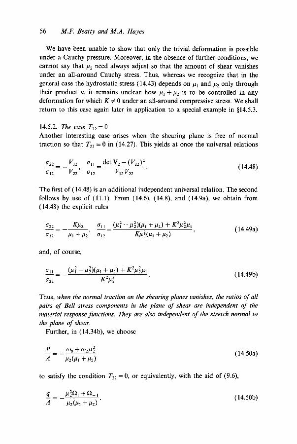
56 M.F. Beatty and M.A. Hayes
We have been unable to show that only the trivial deformation is possible under a Cauchy pressure. Moreover, in the absence of further conditions, we cannot say that #2 need always adjust so that the amount of shear vanishes under an all-around Cauchy stress. Thus, whereas we recognize that in the general case the hydrostatic stress (14.43) depends on/~l and/~2 only through their product x, it remains unclear how /~ + #~ is to be controlled in any deformation for which K # 0 under an all-around compressive stress. We shall return to this case again later in application to a special example in §14.5.3.
14.5.2. The case T22 = 0 Another interesting case arises when the shearing plane is free of normal traction so that T22 = 0 in (14.27). This yields at once the universal relations
0"22 V12 a l l d e t V 2 - (V22) 2 _ - - _ 0"12 V22' 0"12 V12 V22
(14.48)
The first of (14.48) is an additional independent universal relation. The second follows by use of (11.1). From (14.6), (14.8), and (14.9a), we obtain from (14.48) the explicit rules
0"22 K~2 0"11 (#~2-,u~2)(#, +,u2) +K2/~V, - - ~ - - - - - ~ - - ~ a,2 #~ + ~z a~ K#~(~, + ~2) ' (14.49a)
and, of course,
~i, (/~2-/~22)(/~, +#~) + K2#22#I - - = (14.49b) 0"22 K2#32
Thus, when the normal traction on the shearing planes vanishes, the ratios of all pairs of Bell stress components in the plane of shear are independent of the material response functions. They are also independent of the stretch normal to the plane of shear.
Further, in (14.34b), we choose
P 090 + oh#22
A ~ 2 ( ~ 1 - ~ - ~ 2 ) (14.50a)
to satisfy the condition T22 ~--- 0, or equivalently, with the aid of (9.6),
~2t2, + t)_, q - - : A ~t2(~ul + #2) "
(14.50b)
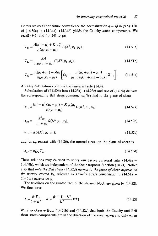
An internally constrained material 57
Herein we recall for future convenience the normalization q = Jp in (9.5). Use of (14.50a) in (14.34a)-(14.34d) yields the Cauchy stress components. We recall (9.6) and (14.24) to get
A(/2~ -/2~ + K~/2~) G(K2 '/21,/2~), (14.51a) TI1 = /2~3/23(/21 +/22)
KA T12 - G( K2, /21, /22), (14.51b)
/22#3(/21 "q- /22)
T33 /23(/21 q-/22) - A/22 [
= ~ - ~ m ~ - ~ ? + - ~ L~I +
/22(/21 +/22) - -#3 A f~_l] (14.51c) /22/23[/23(/21 "1- /22) -- /22 A] J "
An easy calculation confirms the universal rule (14.4). Substitution of (14.50b) into (14.23a)-(14.23c) and use of (14.24) delivers
the corresponding Bell stress components. We find in the plane of shear
(/2~ _ #2~)(#, +/2~) + K2/2~/2, G( K2, /2,, /22), 0"~ = /222(/2~ +/22)
(14.52a)
K2/22 0"22 - - - G( K2, /2~, /22), (14.52b)
/2~ +/22
0",2 = KG(K 2,/2~,/22); (14.52c)
and, in agreement with (14.26), the normal stress on the plane of shear is
0"33 = /21/22 T33. (14.52d)
These relations may be used to verify our earlier universal rules (14.49a)- (14.49b), which are independent of the shear response function (14.24). Notice also that only the Bell stress (14.52d) normal to the plane of shear depends on the normal stretch /23, whereas all Cauchy stress components in (14.51a)- (14.51c) depend on/23.
The tractions on the slanted face of the sheared block are given by (14.32). We thus have
T - /~2T12 /~2 _ 1 -- K 2 N = (KT). (14.53)
1 + K 2' K 2
We also observe from (14.51b) and (14.52c) that both the Cauchy and Bell shear stress components are in the direction of the shear when and only when

58 M.F. Beatty and M.A. Hayes
the shear response G(K 2,/21, ~2) > 0. Then TK > 0 follows from (14.53)~, and hence ( 14.53)2 shows that the sign of N is determined by its numerator term. In the special case when/~ = 1, N = - K T < 0. Thus, the normal traction on the slanted face of a sheared block with equibiaxial stretches/~, = / ~ must be a compression. Moreover, suppose that K ~ 0; then (14.53)2 shows that the normal traction on the slanted face may vanish when and only when /]~ = 1 + K 2, that is, if and only if
~ = #2(l+K2) ~/2. (14.54)
Now consider a unit cube in the undeformed state. Then (14.54), as pointed out by Rajagopal and Wineman [5], shows that in the sheared state of the cube the length #t of the base of the parallelogram of shear is equal to the length/~2( 1 + K 2) ~/2 of the slanted face in the plane of shear. Hence, (14.53)2 shows that the normal traction on the slanted face is a compressive stress N < 0 if and only if the deformed length of the shearing face exceeds the length of the slanted face, and this traction vanishes when and only when these dimensions are equal.
Finally, the case when the plane of shear is free of traction is described by T33 = 0. In this instance (14.26) gives 0"33 = 0, and by choosing p in (14.34c) and q in (14.23c) to satisfy these boundary data, we may derive the Cauchy and Bell stress components. We shall omit these details. We next consider some special cases in further illustration of the shear/stretch problem when
T 1 2 = 0 o r T22=0.
14.5.3. Some special examples Several special cases are possible. One example is a simple shear superimposed on a normal stretch #3 =/~ with equibiaxial plane stretches #~ = #2 = v, an illustration studied earlier in §14.2.1. The stress components for each case described above may be easily obtained.
14.5.3.1. The case T12 = 0. The universal relations (14.38) become
0"12 0"11 0"22 __ __
K 2 2 + K 2' (14.55)
from which we may confirm the familiar Rivlin rule (14.5) in terms of the Bell stress. Thus, all ratios of the Bell stress components in the plane of shear are independent of the equibiaxial strain; they are determined by the amount of shear in the same way for all isotropic Bell materials. The Bell stress compo-

A n in terna l ly c o n s t r a i n e d m a t e r i a l 59
nents (14.37a)-(14.37d) are described by (14.55) in which
a ~ = G ( K 2 , v) = _ f ~ - - f~ ~ . I , : -
(14.56)
Herein we recall (14.24) and (14.9a). Of course, by (14.17) and (14.21), we
shall have f~r = f~r( K2, v). The corresponding Cauchy stress components (14.36a)-(14.36b) become
TI~ = T 2 2 = (D O - Y 2 ( D 2 , T33 = (Do -- ,u(3 -- 2#)(D 2. (14.57)
In order that a shear may be possible under an all-around compressive
stress ~ = T~I = T2~ = T33 given by (14.57)~, we recall by (14.41) that the following relation must hold:
x = v Z = / ~ ( 3 - 2 / ~ ) f o r 0 < / ~ < ~ . (14.58)
Use of the Bell constraint (14.44)~ and (14.58) in (14.45) yields
K2=~(AZ_4x)_ 9(#-1)2 x # ( 3 - 2 ~ ) '
(14.59)
which determines the amount of shear as a function of the transverse stretch alone. The same result follows from the equivalent expression (14.21). We
thus conclude from (14.59) and (14.58) that K = 0 when and only when /~ = v = 1, the undeformed state. Otherwise, the amount of shear grows with the transverse strain under an all-around Cauchy pressure. The graph of (14.59) is parabolic-like; its minimum is the natural state at K 2 = 0,/~ = 1, and
3 the ultimate limit lines for the normal stretch a t / t = 0 and # = ~ are its vertical asymptotes, approached as K 2 ~ ~ . Thus, as /~ increases from 0 to 1, K 2 decreases monotonically from ~ to 0, then it grows again monotonically from
3 0 to ~ as /a varies from 1 to 3. Finally, we need to recall the principal stretch condition that either 21 = 23
or 22 = 23 in order that T~2 = 0 for (D2 ~ 0 in (14.40). The principal stretches are given in (14.17), and it is certainly not evident that our condition is satisfied. We see, however, that (14.58) and (14.59) yield v2K2= 9 ( # - 1) 2. Thus, by (14.17), it may be verified that, indeed, 2~ = 23 =/~ and 22 = 3 - 2/~, or vice versa. Therefore, we find, in accord with the Bell constraint (3.1), the principal stretches
2 1 = 2 3 = ~ , 2 2 = 3 - 2 # , (14.60)
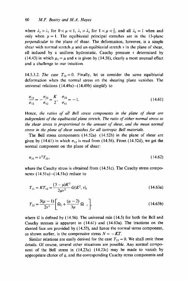
60 M.F. Beatty and M.A. Hayes
where 22 > 21 for 0 </~ < 1, R~ > )-2 for 1 < # < I, and all 2k = 1 when and only when /~ = 1. The equibiaxial principal stretches are in the 13-plane perpendicular to the plane of shear. The deformation, however, is a simple shear with normal stretch/~ and an equibiaxial stretch v in the plane of shear, all induced by a uniform hydrostatic, Cauchy pressure r determined by (14.43) in which #3 =/~ and x is given by (14.58), clearly a most unusual effect and a challenge to our intuition.
14.5.3.2. The case T22 =0. Finally, let us consider the same equibiaxial deformation when the normal stress on the shearing plane vanishes. The universal relations (14.49a)-(14.49b) simplify to
0"11 0-22 K 0"22 - - 2 ' - - = - 1 " ( 1 4 . 6 1 )
0"12 O'12 0"11
Hence, the ratios of all Bell stress components in the plane of shear are
independent of the equibiaxial plane stretch. The ratio of either normal stress to
the shear stress is proportional to the amount of shear, and the mean normal
stress in the plane of shear vanishes for all isotropic Bell materials.
The Bell stress components (14.52a)-(14.52b) in the plane of shear are given by (14.61) in which 0"12 is read from (14.56). From (14.52d), we get the normal component on the plane of shear:
0"33 = •2T33 , (14.62)
where the Cauchy stress is obtained from (14.51c). The Cauchy stress compo- nents ( 14.51 a ) - ( 14.51 c) reduce to
(3 - #)K 2 G(K2 ' v), (14.63a) TI~ = KT12 - 2/~v 2
T33 3 ( # - 1 ) I f ~ l + ~ 2 ) f ~ 2 v 2 i1, (14.63b)
where G is defined by (14.56). The universal rule (14.5) for both the Bell and Cauchy stresses is apparent in (14.61) and (14.63a). The tractions on the slanted face are provided by (14.53), and hence the normal stress component, as shown earlier, is the compressive stress N = - K T .
Similar relations are easily derived for the case T33 = 0. We shall omit these details. Of course, several other situations are possible. Any normal compo- nent of the Bell stress in (14.23a)-(14.23c) may be made to vanish by appropriate choice of q, and the corresponding Cauchy stress components and

An internally constrained material 61
traction conditions may be determined. Introduction of special response
functions will also yield further special results.
This completes our study of the shear/stretch problem. We next examine a significant related example.
15. Finite twist and axial stretch of a thin-walled tube
For finite torsion-tension experiments in which thin-walled, cylindrical tubes of annealed copper, mild steel, and aluminum were severely twisted and
extended, Bell [2, 18] has reported recently the remarkable empirical result that the rigid rotation of the principal axes of V is negligible, so that to a close approximation the rotation R =" 1. All tubes were bored to 0.375 in. inside
diameter, and their wall thickness was either 10% or 15% of the mean radius R,,. The data provided in [2] indicate that the average value of the mean diameter for 12 tubes was Dm = 2R,, = 0.4043 in., their average length was
L0 = 4.212 in., so their corresponding average slenderness ratio w a s Z o / D m =
10.4. The tubes were loaded nearly to failure, or to failure, 2 without reverse loading or unloading along any of the various stress paths, and measurements
were made under load in this ultimate configuration. In one example, the twist was 347 ° with an axial extensional strain of 24%; yet the rigid rotation was only 6.91 ° , minuscule in the context of the gross deformation of the tube.
Similar results are noted for finite bending of cantilevered beams. We shall now show that our results for shear with triaxial stretch are related to Bell's
kinematical study of experimental data derived from these trials. We begin with the kinematics of the thin-walled tube approximation, and afterwards examine the kinematical effects of the small rigid rotation and other experi- mentally based approximations.
15.1. The thin-walled tube approximation
We first note that the nonhomogeneous deformation for the finite twist and stretch is described by the cylindrical coordinate relations
r=~R, O = ® + ~ Z , z = r Z , (15.1)
in which the point of the tube at (r, 0, z) in its current configuration was at the place (R, 19, Z ) in the undeformed state. The stretches ~ and 6, and the total
2 Bell [18] characterizes failure as the onset of highly localized, nonhomogeneous axial necking, or the formation of equally highly localized shear bands. Either situation was followed by immediate flow and failure of the grossly deformed state of the tubes.

62 M.F. Beatty and M.A. Hayes
angle of twist ~b, per unit undeformed tube length Lo, are constants. For a thin-walled tube with undeformed mean radius Rm, introduction of R-" R,, into (15.1) yields deformation relations of the form (14.1) in which, following Ericksen (see Bell [18]), we identify (x, y, z) ~ (rO, z,r), (X ,Y ,Z)~ (R®, Z, R), and
fl l = 1-/3 -~- ~ , /22 ~ 6 , K=~k, (15.2)
where k = R,AO. Thus, with (15.1)~,
6K = ~k = ~R,~ ~ = r,~ ft. (15.3)
Therefore, the finite twist and extension of a thin-walled tube is described in these terms as a shear with equibiaxial stretch in the shearing planes perpen- dicular to the axial extension. In this case, the kinematical relations given in (14.2)-(14.16) are applicable, regardless of any constitutive properties of the Bell constrained material.
It can be shown that the orthogonal shear of the X and Y material lines, in accordance with equation (26.10)1 in [17], is determined by the familiar rule known for a simple shear of amount K. Thus, with the use of (15.2)3, the angle of shear I~12 is given exactly by
tan [ '12 = K = ~ k. (15.4)
Moreover, k and K have similar geometrical interpretations. Consider a point P on the circle of mean radius rm = ~Rm distant z = 6Lo
from the base of the tube and lying on a coaxial generator ~ . When the tube is then twisted about its axis through a total angle ~ relative to the base, ~ is deformed into a helical line. The pitch triangle of the helix is a right triangle with height ~r,~ = ~R,~ perpendicular to its base ~ of length 6Lo. Therefore, recalling (15.2)3, we see that the tangent of the helix angle v from ~ is
tan v - ~ g R . , _ c t O R , ~ _ ct k = K ; ( 1 5 . 5 ) 6Lo 6 6
that is, the helix angle v = I ~ 2 is the finite angle of shear in (15.4). Similarly, we see that the helix angle 7 in the total twist of angle ~ of a cylindrical surface of radius R m and length Lo is given exactly by
~Rm tan 7 = = R,,~k = k. (15.6)
L0

An internally constrained material 63
Hence, 7 = ?~2 is the angle of shear in a pure twist of the circle of radius Rm. Indeed, it can be shown with the aid of equation (26.10)2 in [17] that two material lines separated by an angle LI/12 in the undeformed state are sheared an amount k into orthogonal lines in the deformed state where the included angle is ~12 = re/2 and hence ~12 = ~FI2-~/12 is the angle of shear. These results are useful in visualization of the experimental results discussed by Bell [2, 18].
Exact expressions for V and R may be obtained from (14.6) and (14.12) upon use of (15.2). We thus find
1 V = ~ ([oe(oe + 3) + K232]ell + ~(oe + 6)e22
+ K62(ei2 + e2~)) + oee33, (15.7)
1 R=~[(~+6)(e11+e22)+K3(e12-e21)]+e33,
wherein, by (14.9a),
A = x//(o~ + 6) 2 + K232.
(15.8)
(15.9)
Also, use of (15.2) and (15.3) in (14.13) delivers the exact relation for the rigid rotation angle ~b,
6K ~K rm~ tan~b ~ + 6 ~ + 6 ~ + 6 " (15.10)
This may be confirmed also from (15.8). Indeed, in terms of the rotation angle in (15.10), (15.7) and (15.8) may be written as
V = (~ + 6 sin 2 40 sec 4~e1~ + 3 cos ~e22
(15.11) + 3 sin ~b(el2 + e21 ) + oee33 ,
(15.12) R = cos 4~(ell + e22) + sin q~(el2 -- e21 ) + e33.
The constraint (14.14) becomes
= 3 - x/(o~ + 6) 2 + ~2k2 = 3 - (~ + 6) sec ~b; (15.13)
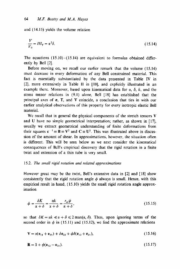
64 M.F. Beatty and M.A. Hayes
and (14.15) yields the volume relation
1/ 77, =IIIv = ~2~. (15.14) Vo
The equations (15.10)-(15.14) are equivalent to formulas obtained differ- ently by Bell [2].
Before moving on, we recall our earlier remark that the volume (15.14) must decrease in every deformation of any Bell constrained material. This fact is essentially substantiated by the data presented in Table IV in [2], more extensively in Table II in [18], and explicitly illustrated in an example there. Moreover, based upon kinematical data for ~, 3, k, and the stress tensor relations in (9.1) alone, Bell [18] has established that the principal axes of it, T, and V coincide, a conclusion that ties in with our earlier analytical observations of this property for every isotropic elastic Bell material.
We recall that in general the physical components of the stretch tensors V and U have no simple geometrical interpretation; rather, as shown in [17], usually we extract geometrical understanding of finite deformations from their squares c- ~ = B = V 2 and C = U 2. This was illustrated above in discus- sion of the amount of shear. In approximations, however, the situation often is different. This will be seen below as we next consider the kinematical consequences of Bell's empirical discovery that the rigid rotation in a finite twist and extension of a thin tube is very small.
15.2. The small rigid rotation and related approximations
However great may be the twist, Bell's extensive data in [2] and [18] show consistently that the rigid rotation angle ~b always is small. Hence, with this empirical result in hand, (15.10) yields the small rigid rotation angle approx- imation
6K ~k r,,~ - - _ _ - - ~b ~ + 6 ~ + ~ ~ + 6 ' (15.15)
so that 6K = ~k ,~ ~ + 6 ~< 2 max(a, 3). Thus, upon ignoring terms of the second order in ~b in (15.11) and (15.12), we find the approximate relations
V = ~x(e~, + e33 ) -t- &e22 + ~b6(et2 + e21), (15.16)
R = 1 + ~b(et~ - e2~). ( 1 5 . 1 7 )

An internally constrained material 65
Therefore, the internal constraint for a finite twist and extension of a thin-walled tube with a small rigid rotation, according to (15.16) or (15.13),
becomes
tr V = 2~ + 6 = 3. (15.18)
Notice that the same thing follows from (15.13) when q~ in (15.15) is small. The right stretch tensor U = RrVR also may be approximated from the relations (15.16) and (15.17). To the first order in ~b, we have
U = ~(e,1 + e33) -k c5e22 q- ~b(e~ + e21 ). (15.19)
The thorough experimental data presented by Bell [2, 18] support his remarkable empirical discovery based on (15.15) that in any finite twist and extension of a thin-walled cylindrical tube R -" 1, very nearly. It is shown in [18] that the data for 85 tests obtained at the maximum deformation prior to failure, tests in which rigid rotation is taken into account, yield a measured average value of tr V = 2.9998. However, when the approximation (15.17) is introduced, the computed value obtained from (15.18), based on the average ultimate values ~=.9581, 6=1 .078 provided in Table I in [18], is tr V = 2.9942, a value smaller than the actual average measured value by merely 0.19%.
In addition, it may be seen from this tabulation that three further approx- imations are accurately supported by Bell's data. Accordingly, these data show that the angles of shear in (15.4) and (15.6) and the shear component of V in (15.16) are approximated by
7~2 "-- k, F~2 _'- K, 4~6 -' ~1~ 2 " ( 1 5 . 2 0 )
Hence, in view of (15.4), we have also
1~12 --" ~ "~12 • (15.21)
The composition of the experimentally motivated approximations (15.20) and (15.21) shows that
I~12 ~b "- 2 (15.22)

66 M.F. Beatty and M.A. Hayes
As consequence of (15.20) and (15.22), all the terms in (15.19) now have familiar geometrical interpretations; but the deformations are not infinitesi- mal. In general, of course, to the first order in q~, (15.21) shows clearly that ~)12 :~ F~2, which is to be expected in view of our earlier geometrical interpreta- tion of these angles of shear. Though generally distinct, it certainly is possible that one may closely approximate the other in accordance with (15.21).
We find, in fact, for the various quantities in (t5.20) and (15.22) the following average values determined from the 85 tests described by Bell [18]:
Table L Hypothetical model data based on average values of 85 tests reported by Bell [18].
6 ~b ~12 k 2~q~ F12 K 2~b
.958 1.077 .0683 .144 .145 .147 .129 .130 .131
We note that ~ is given in radian measure (3.916°). Since Bell's data [18] provide only a single data point for each of 85 specimens under different loading conditions at an ultimate state prior to failure, these average values are intended only as a hypothetical model of a typical kinematical state without bias toward a particular test. It is appreciated, of course, that such average values generally may not be meaningful. In some cases they are. The linear relation (15.18), for example, must hold for each test, and hence the average value of tr V and its value computed from the average values of ~ and 6 must be the same, as shown earlier. As a final check, we calculate for our average model (~/6)k =0.129 and tan I~12 = .129, which according to (15.4) also should equal K above; and (~/6)712=0.128, which by (15.21) should closely approximate F~2. We thus find excellent agreement. Calculations for individual data points in [18] naturally will vary, but they are nonetheless consistent with our example. Thus, as shown by Bell [2, 18], his experimental data accurately support the small rigid rotation and the related approxima- tions presented above in (15.20)-(15.22). We shall return later to Bell's important result that R - 1 in our further discussion of the torsion problem.
Finally, it will prove useful to observe a further approximation. In view of (15.20) and (15.6), it is seen that
0 rmdg = aRm Z00 = °~])12' ( 1 5,23)
very nearly. Thus, for later use, we observe that
r2~b 2 ,~ (3 -- ct) 2 ,~ ~2722 '~ (3 - ~)2. (15.24)

An internally constrained material 67
Indeed, for our averaged data example, [~12/(3-~x)] 2 =0.005. It may be helpful to recall that Lo/R,, "- 20.
With the thin-walled tube and small rigid rotation approximations in hand, we now turn to the stress distribution for our problem.
15.3. Stress in a thin-walled tube under finite tw&t and stretch
The Cauchy stress distribution in the finite twist and extension of a thin- walled tube for which R " - - R m may be read from (14.34). With the index notation adjusted so that (1, 2, 3) -~(0, z, r), use of (15.2) and (15.3) in (14.34) yields the following physical components of the Cauchy stress in terms of cylindrical reference coordinates:
Trr = p~ +mo + m2~ 2, (15.25a)
Too = ~ (o¢ z + ~6 + r2~ff 2) + ¢oo + ¢o~(~ 2 + r~mff2), (15.25b)
P (a ~ + ~6) + o~ 0 + (D2 ~2, (15.25c)
To: = T.~o = ( ~ q- ~O2 )6rm~ t, (15.25d)
wherein, with (15.9),
A = 3 - ~ = x/(~ + 6) 2 + rZ,,ff 2. (15.26)
The reader may obtain the corresponding Bell stress components from (14.23). We recall that only one universal rule is obtained from (8.1), namely (14.4), which has the form
To o _ T~ z o~2 - - ~)2 q_ r2m~2
To~ 6r,.~b (15.27)
The traction relation on the radial surfaces will require (14.26) and (14.27); (14.28) is needed for the end conditions. Before addressing these matters, however, we shall need to recall the engineering stress tensor in (9.1), namely, TR = JTF -r . Introduction of the thin-walled tube approximation embodied in (15.2) and (15.3) into (14.2) yields
1 rm~ J = d e t F = ~ 2 6 , F - ~ = l ( e r R + % o ) + e:z (15.28) %z,

68 M.F. Beatty and M.A. Hayes
where ekL = ek ®eL is the mixed physical tensor product basis for which L = 1, 2, 3 respectively correspond to O, Z, R. Hence,
T R = ct6TrrerR + ~t(6Too - rm~k Toz)eoo + ~2T~zezz
+ ct2To~eoz + o~(6Toz - r,,~kT~z)eze. (15.29)
The undetermined constraint parameter p in (15.25) may be chosen to satisfy any condition involving the stress components. Thus, following 3 Bell [18], we choose p so that e0 • TRee = 0 in (15.29), that is, so that
TR<0e> = ~(6Too - rm d/Toz) = 0. (15.30)
Use of (15.25b) and (15.25d) in (15.30) yields
P - c°°+~2c°2 (15.31) A ~(~ + 6)
Thus, noting (15.26h, we see that the Cauchy stress components in a thin-walled tube under finite twist and extension become
__ 3) T,r \ ~ t + f (09°+ct2~°2)' (15.32)
T~ = (~--~)(COo - ~5co2), (15.33)
and Too and To~ are provided by the universal relations (15.27) and (15.30). We thus obtain the universal rules
Too rm~/ Tzz 52--ct 2 Too r~b 2
Toz 6 ' Toz 6 r , . ¢ ' T= 6 2 - ~ 2" (15.34)
These relations may be expressed in other terms by use of (15.3). In particu- lar, it is seen that Too = KToz, which is equivalent to (15.30).
3 Bell uses Exx, Exr . . . . , to d e n o t e the phys ica l c o m p o n e n t s o f the eng inee r ing s t ress t enso r
T R. In o u r te rms, the r eade r will f ind t h a t TR<rR>=EZZ, TR<OO>=~,rr, TR<zZ>=~,xx, TR<oz > = Zrx + ~t, TR<~o> = Ext.
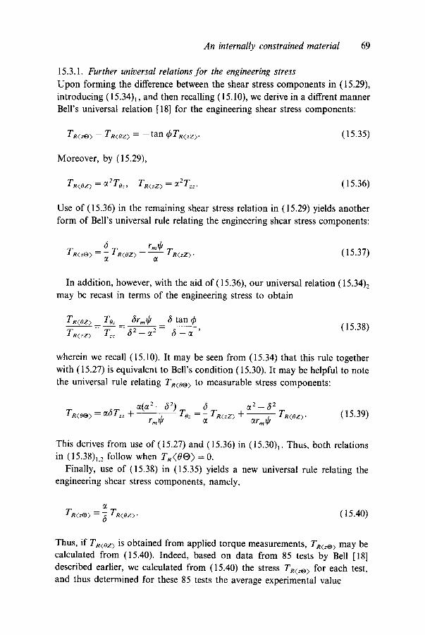
An internally constrained material 69
15.3.1. Further universal relations for the engineering stress Upon forming the difference between the shear stress components in (15.29), introducing (15.34)1, and then recalling (15.10), we derive in a diffrent manner Bell's universal relation [18] for the engineering shear stress components:
TR<~O> -- TR<oz> = -- tan c~TR<zz>. (15.35)
Moreover, by (15.29),
TR<oz> = ~2Toz, TR<zz> = ~2T=. (15.36)
Use of (15.36) in the remaining shear stress relation in (15.29) yields another form of Bell's universal rule relating the engineering shear stress components:
c~ rm¢ TR<zo> = ~ TR<oz> -- T TR<zz>. (15.37)
In addition, however, with the aid of (15.36), our universal relation (15.34)2 may be recast in terms of the engineering stress to obtain
TR<OZ > Toz (~rm~l ~ tan ~b - - , (15.38)
TR<:Z> T= 62 _ ~2 6 --
wherein we recall (15.10). It may be seen from (15.34) that this rule together with (15.27) is equivalent to Bell's condition (15.30). It may be helpful to note the universal rule relating TR<0o> to measurable stress components:
~(ot 2 - - c~ 2) To z 6 c~ 2 - 62 TR<0o> = c~6T~: -t rm~ = ~ TR<:z> + ~ TR<oz>. (15.39)
This derives from use of (15.27) and (15.36) in (15.30)1. Thus, both relations in (15.38)1.2 follow when TR(O0) = O.
Finally, use of (15.38) in (15.35) yields a new universal rule relating the engineering shear stress components, namely,
TR<zo> = ~ TR<oz>. (15.40)
Thus, if TR<oz> is obtained from applied torque measurements, TR<zo> may be calculated from (15.40). Indeed, based on data from 85 tests by Bell [18] described earlier, we calculated from (15.40) the stress Tn<~o> for each test, and thus determined for these 85 tests the average experimental value

70 M.F. Beatty and M.A. Hayes
TR<zo> = 8.545 kg/mm 2. In addition, we find that (15.35) and (15.37) yield comparable values calculated from Bell's data. The average value predicted by (15.35) is 8.625 kg/mm 2, and with (15.37) is 8.729 kg/mm 2. The former is 2.1% greater, the latter less than 1% larger than the average computed from (15.40). If the average value for TR<oz > = 9.345 kg/mm 2 calculated from Bell's data is used for our hypothetical model described in Table 1, (15.40) yields T~<~o> = 8.312 kg/mm 2, which is 2.8% smaller than its actual average value.
The consistency as regards the Bell condition expressed in (15.38) is not as nice. While the kinematical relations in (15.38) agree very closely in all the tests, the comparison with the stress ratio on the left-hand side of (15.38) often is poor and varies from one test to another, sometimes considerably. In the sense of our hypothetical model, for example, the variance is about 38%. Alternatively, using (15.39)2, we have also calculated from Bell's data an average value of T~<0o> = -3.109 kg/mm 2. For our hypothetical model, the same stress determined from the averaged data values found for each term in (15.39)2 is -4.679 kg/mm 2. These average values for T~<0o> are of the order of 30-40% of the average measured shear and axial engineering stress components in (15.38). We find it nonetheless astonishing that our theoretical results derived from nonlinear elasticity theory for an isotropic elastic Bell constrained material should agree so closely, in general, with Bell's data for finite plastic strain of metals. And there is more to follow.
15.3.2. Traction conditions for a thin-walled tube It is important to recognize that so far we have used only the thin-walled tube approximation together with Bell's condition (15.30). We now consider the null traction condition on the cylindrical tube surfaces. By (14.26), this requires Trr = 0 in (15.32). This will hold for all isotropic Bell materials if and only if the radial stretch ~ and the axial stretch 6 satisfy the rule
2e + 6 = 3. (15.41)
That is, we must have ~ ~ (0, -~) and 6 ~ (0, 3). Now, in order that this may be compatible with the kinematical constraint (15.26), it is necessary that the twist satisfy
r~b e ~ (~ + ~)= = (3-- ~)2 = A 2. (15.42)
This is the only restriction we need impose on the twist ~b, which may be substantial. Indeed, consistent with (15.41), the right-hand side of (15.42) is least when ~ =~, and hence rm~l = O~0`Rm/L o '--30"/40 ,~ 3/2 requires that the total angle of twist 0" ,~ 20 radians! When ~ is close to one, the twist consistent

An internally constrained material 71
with the null traction data may be considerable. Nevertheless, in accordance with (15.10), (15.42) implies that tan q~ ~ 1, that is, the rigid rotation angle must be small. In consequence, (15.10) may be replaced by (15.15), and use of (15.41) shows that
I'm~l r,,O 2r., 0 4~ a + 6 - 3 - - ~ 3 + 6 "~1" (15.43)
We thus deduce Bell's remarkable experimental result that in the finite torsion and extension of thin-walled cylindrical tubes for which (15.30) holds, the rigid rotation of the coaxial principal axes of V, T, and ~ must be very small, and hence to a close approximation R-" 1. We recall that (15.42) is the same as (15.24), which was shown to hold for the model data described in Table 1. In this case, the reader will find with the aid of (15.23) the angle of twist 0-" 2 . 8 8 r a d = 165 °, for example, while the rigid rotation angle ~b= .068 rad "--4 °, certainly quite small compared with the gross deformation of the tube in this model case.
We recall that our earlier analysis of the kinematics of small rigid rotations in §15.2 led naturally to the Bell constraint (15.18), precisely the condition (15.41) for traction free lateral surfaces. Therefore, in accordance with (15.32), we conclude that the lateral surfaces of a thin-walled cylindrical tube under finite twist and stretch may be traction free for all isotropic Bell constrained materials if and only if the rigid rotation of the coaxial principal directions for ¥, T, and ~ is small.
Of course, the equilibrium equations also must be satisfied. For a given finite twist and stretch, the physical stress components (15.32), (15.33), and (15.34) are constant. In view of (15.43), it may be seen that the equilibrium equations are satisfied approximately to o(~b2).
Further, if virtually no axial force is supplied on the ends of the tube so that T~ = 0, very nearly, it follows from (15.33) that
e = 6 = 1, very nearly. (15.44)
The reader will find that this result is consistent with Bell's observations recorded in [18, p. 5]: "When measuring the inside and outside diameters of thin-walled tubes in simple twisting in absence of axial forces, an unantici- pated discovery was made. Completely unexpectedly, it was found that inside and outside diameters of tubes, simply twisted without axial load, remain unchanged to four decimal places, even for angles of twist in excess of 300°." Thus, to a high order of accuracy, Bell finds ~ = 1. And in the subsequent paragraph in [ 18], he writes "that for large finite strain plasticity in cylindrical cross-sections, plane sections remain plane." Thus, this response is consistent

72 M.F. Beatty and M.A. Hayes
with ~ = 1, very nearly, in (15.44). Of course, we learned long ago that a simple torsion for which (15.44) holds exactly is impossible in any Bell constrained material. Therefore, we feel that Bell's empirical observations in this case are consistent with our analysis in the context of nonlinear elastic material response provided that these data be interpreted in the sense of close approximation in (15.44).
15.3.3. Further observations
Introduction of (15.43) into (15.34)2, and use of (15.20)3, (15.33), and (15.41) yields
~ _ ~t2 d, L z = ( 6 - = - T o z = (15.45)
where the shear response function d(IIv , IIIv) is defined by
~ = I ( -090 + ~&o2). (15.46)
If the A-inequalities (6.11) hold, ~ > 0. Therefore, according to (15.45), in
every finite twist and stretch of a thin-walled tube with traction free lateral mantel, the A-inequalities imply that the shear stress is in the direction of the
shear ~2 and the axial stress is in the direction of the stretch 6. Thus, further, i f the tube is elongated, then 6 > 1 (shortened 6 < 1), ~ < 6 (~ > 6) in (15.45), and in accordance with (15.41), the tube wall must contract with ~ < 1 (expand
with ct > I). The total force N and total torque M applied to the ends of the tube are
given by
N = Ao~2Tzz = AoTn<zz>, M : Aormot2Toz = Ao~XRmTr<oz >, (15.47)
in which (15.36) is recalled. Hence, with the aid of (15.10) and (15.47), the universal formula (15.38) for the finite twist and stretch of a thin-walled tube relates the axial force to the torque in accordance with
N r~ T~<~z> ~ - o~ ~2 _ ~2 (15.48) - -
M rmToz ~R,,Tn<oz > r~o~R m t a n ~b 6~2R2m~k "
Thus, further, with the small rigid rotation approximations in mind, we may use the Bell constraint (15.41) and (15.43) to write (15.48) in terms of the twist and stretch alone. This yields for the finite twist and stretch of a

An internally constrained material 73
th&-walled tube with null lateral tractions the un&ersal rule
R2mN 3 ( 3 - 1 ) ( 6 + 3 ) ~(6) 62(3 - 6) 2
(15.49)
relating the torsional modulus z(~) = M/(~b /6) to the axial force and the stretch in the same way for every isotropic, elastic Bell constrained material. The function (15.49) is monotone increasing from - ~ at 6 = 0 to + ~ at 6 = 3, vanising at 6 = 1. The two terms in (15.49) may be calculated independently for each of Bell's 85 tests recorded in [18]. We find that the averaged data for the two sides of our universal relation (15.49) differ by only 2.2%.
This concludes our primary investigation of this problem. We now direct attention toward the development of constitutive equations for hyperelastic Bell materials.
16. Isotropic, hyperelastic Bell materials
There is nothing in our previous study that depends upon the existence of an elastic potential for the stress working, and we have had no need to appeal to the mechanical energy principle. In this section, we now introduce the concept of the elastic strain energy function E for an isotropic material. The mechan- ical energy principle [6, 14] is then applied to derive the constitutive equation for an isotropic, hyperelastic Bell material. The response functions will thus appear in terms of certain derivatives of Y~. The A-inequalities restricting the strain energy function will also be expressed in these terms, and compatibility equations for the response functions will be derived. Special material models suggested by the compatibility relations will be described, and their applica- tion in an important special case discovered by Bell and described in experi- ments by himself and others [1] will follow.
An isotropic, hyperelastic material is characterized by an isotropic, scalar valued function E = E(Iv, IIv, IIIv), the strain energy per unit volume V o in Xo. This function must satisfy the principle of mechanical energy balance ex- pressed in the differential equation
~ = J tr(TD), (16.1)
wherein we recall (2.1), (2.2), and note that the right-hand side of (16.1) describes the rate of working of the Cauchy stress T. For a material con- strained by (2.5), however, the strain energy determines the stress only to within an arbitrary workless stress (4.2) which, by (4.1), contributes nothing to (16.1). Thus, in view of the Bell constraint (2.4), we consider E=

74 M.F. Beatty and M.A. Hayes
E(IIv, IIIv) in (16.1) and note that the material time derivative of E yields
dE dE Z = ~ [Iv tr ~ - tr(V2D)] + ~ J tr D.
Bearing in mind the constraint (2.5) and introducing the last result into (16.1), we obtain the relation
[ 1 0x T - oIIIv + ~ OIIv j-D=0
valid for all symmetric D for which (2.5) holds. It thus follows that the constitutive equation for an isotropic, hyperelastic Bea material is given by
~X 1 1 ~E V2" (16.2) T = p V + ~ ~
Alternatively, introducing th~ Bell stress (9.1) into (16.2), we find
~ = q l - V + I I I v ~ V -~, (16.3) V ~ l l l v
in which the undete~ined constraint parameter q = Jp. An alternative derivation of (16.3) may be constructed in t e ~ s of the
principal reference system. We write ~(IIv, IIIv)= ~(2~, 2~, 2~), where X~ are the principal stretches subject, of course, to the constraint 2~ + 2~ + 2~ = 3. If variations in 2~ are denoted by ~ , then the constraint £~ ~ ~ 82~ = 0; and in the principal reference system for V, the principle of virtual work yields
3 3
6~= 2 T~32~-0 2 62k, (16.4) k = l k = l
in which T~ are the principal forces and ~ is a Lagrange multiplier. Thus, (16.4) yields for all 62, the rule
~£ T, = ~ +~. (16.5)
Thus, ~ t h £ = Z(IIv, IIIv) and recalling (9.9)~, we obtain
0X 0X ~ ~k =~ + 3 0 ~ ~ v 2~ + IIIv v 2 ; ' (16.6)

An internally constrained material 75
in the principal reference system for V, and hence also for 6. Upon writing q =- ~ + 3 OZ/OIIv, we recover (16.3) in the common principal system o f o and
V, and hence for all reference systems. Comparing (16.2) and (16.3) with the corresponding formulae (5.11) and
(9.5) for an isotropic, elastic Bell material, we see that the response functions c06 and Dr may be expressed in terms of the strain energy as follows:
~E 1 ~E ~o~ = - ( 1 6 . 7 )
e~o - ~IIIv' IIIv ~IIv'
~E ~E ~ 1 = I I I v ~ 2 - - ~IIv' ~ - ~ = I l l v ~ ° = I I I v OlIIv" (16.8)
The formulae (16.8)L 3 agree with our earlier relations in (9.6); and the A-inequalities (9.7) are equivalent to
0Z 0Z 0-~v < 0, ~-~v ~< 0. (16.9)
In view of (3.2), the inequalities (16.9) confirm that the strain energy must increase as the invariants decrease from their maximum values in the undistorted
state. The following compatibility relations derive from (16.7) and (16.8):
v
~ v + (IIIvco2) = 0, (16.10)
~Q_1 ~Q] - - + IIIv - 0 . (16.11) ~ IIv ~ IIIv
Some special results may be read from these equations. It is seen from (16.11) that
(i) ~ r = f~r (IIIv) ~ ~1 = a, constant, ~ - ~ = f l - 1 (IIIv), (16.12)
(ii) D r = ~ r ( I I v ) = ~ l = b , constant, ~ =fl~(IIv) , (6.13)
wherein F = 1, - 1 . Also, with (16.8)1,3 , (16.12) implies also that
a
(iii) c% = oo~x(IIIv ) .~ co2(IIIv ) - I I Iv ' (16.14)

76 M.F. Beatty and M.A. Hayes
with A = 0, 2, a result that follows also from (16.10) directly. On the other hand, (16.8)j.3 and (16.13) yield only
b f~,(IIv ) COo(IIIv ) -- IIIv' CO2(IIv, IIIv ) = I I I v (16.15)
Other possibilities also are evident. A constitutive equation for a specific isotropic, hyperelastic Bell material described by Bell [1] will be studied next.
17. Bell's law
We see that (16.13) includes the special Bell material described by (13.19) or (13.20) for which f~_~ = 0 or COo = 0 in (16.8). In this case, the strain energy E = Y(IIv) depends on only IIv and with (16.7) and (16.8), the single response functions in (13.19) and (13.20) are respectively determined by
dY~(IIv ) (17.1) ~.~1(ii¥)_ dZ(IIv_~___)dliv ' co2(IIv' IIIv ) = - I I I ~ dIIv
To complete this model, however, and to connect the theory with the abundant experimental data due to Bell and others [1, 2, 7, 9], we need to know the form of the strain energy function E(IIv). We turn again to Bell's experimental results. Bell [ 1] has shown that all of his tests are consistent with the specific work function 4
~,(IIE) = ~ ( - 2IIE )3/4 = ~[2(3 - IIv )13/4 = E(IIv). (17.2)
Herein fl is a material constant. Also, we recall (3.2) and (3.9a) relating the invariants:
- - l i e = 3 - - I I v > 0 . (17.3)
We thus determine from (17.1) and (17.2) the response functions for the isotropic materials, all primary metals, studied by Bell, namely,
~ = r[ 2( 3 - IIv )] - ~/4 = r( _ 2IIE ) -~/4, (17.4)
092= I I I ~ 1 ~ =(1 +I IE + I I I E ) - ~ , (17.5)
4 Our invariant II E is the negative of Bell's IlE.

An internally constra&ed material 77
in which (3.9b) is used. We select the form (17.4) and recall (13.19) to deduce a new constitutive equation called Bell's Law:
~ = ql ÷/3V[2(3 - IIv )] - 1 / 4 (17.6)
Alternatively, with the aid of (3.8) and an adjusted normalization, we get
o = ~1 + / / E ( -2IIv~ ) -1/4, (17.7)
in which ~ is another undetermined constraint parameter. To our knowledge, these constitutive equations are herein presented for the first time. Their premiere application in three examples related to Bell's experiments follow.
It is clear that (17.6) cannot apply in the neighborhood of the undeformed state. Bell has shown, on the other hand, that away from the undeformed state, the material response is indeed modeled by (17.6).
17.1. Application of Bell's law to uniaxial loading
Let us begin with the uniaxial loading problem studied in §8 and §9.2. We recall the axial strain E = 2 - 1 and note that (8.12)1 and (17.3) yield
3 2 3 2 IIv= 3 - z E , IIE= - ~ E . (17.8)
Hence, (17.4) delivers the response function for the uniaxial loading case:
f~, =f~(E) =y]EI-'/2 with 7 =/~(~) I/4 (17.9)
Therefore, the uniaxial Bell stress is determined by (9.16). Indeed, we observe that (17.9)~ is exactly the result needed in (9.19). We thus derive precisely Bell's parabolic law for uniaxial loading given in (9.18). Moreover, in (17.9)2, we determine exactly the material parameter ~ described in Bell's experiments [ 1].
17.2. Application of Bell's law to pure shear
Now let us consider the pure shear problem studied in §13. We recall (13.5)~ and use (17.3) to obtain the invariants
I Iv= 3 - E ~ , IIw= - E ~ (17.10)
for a pure shear with E3 = - E~, E2 = 0. Then (17.4) yields immediately
f~, =O(]E,]) =~tlE,] -'/2 with ~ _= 2-'/4fl, (17.11)

78 M.F. Beatty and M.A. Hayes
and hence the Bell stresses are provided by (13.16). We observe, in fact, that (17.11)~ is precisely the result needed in (13.18). We thus derive exactly Bell's parabolic law for pure shear given in (13.17), and in (17.11)2 we provide precisely the material parameter ~ characterized in Bell's work [ 1].
17.3. Bell's &variant parabolic law
Another example of a more general nature which is connected with Bell's research studies on large deformations of metals will be described next. Bell [1] has introduced a deviatoric stress tensor S defined by
S -- t~ - ½(tr ~)1, (17.12)
so that tr S = 0 , and two invariant 5 quantities T and F, the deviatoric stress and strain intensities, defined by
T - - ~ = x / ~ , r = ~ = ~ . (17.13)
It is seen from (17.7) that tr t~ = 3~, and thus S = ~ - 01 is the extra Bell stress tensor. We notice also that, geometrically, F is the magnitude (3.11) of the principal engineering strain vector, the position vector from the undistorted state in the invariant triangle to a point on the principal deformation trajectory
in the invariant plane, the plane defined by tr E = 0. We seek a relationship connecting the deviatoric stress intensity to this strain intensity measure.
Upon substitution of (17.7) into (17.12) and use of the Bell constraint
(3.10), we deduce the constitutive equation relating Bell's deviatoric stress to the deviatoric strain, namely,
S = flF-~/2E. (17.14)
This is the deviatoric, or extra stress, form of Bell's law in (17.7). Hence, S 2 =fl2F-~E2 and from (17.3) we thus derive Bell's invariant parabolic law relating the deviatoric stress intensity to the corresponding strain intensity:
T 2 = fl2F. (17.15)
The graph of T 2 versus F is a straight line of constant slope characteristic of the Bell material. In particular, for annealed copper, Bell reports f l= 37 kg/mm 2 obtained in a variety of experiments in which various ratios aE/a~ of the principal Bell stresses are controlled. These data are shown as Fig. 3 in [1].
5 These invariants differ in sign from those defined by Bell.
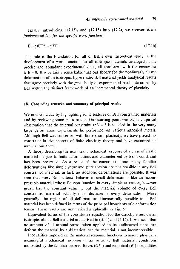
An internally constrained material 79
Finally, introducing (17.13)2 and (17.15) into (17.2), we recover Bell's fundamental law for the specific work function:
E =3//F2 3/2 = 32_ TF. (17.16)
This rule is the foundation for all of Bell's own theoretical study in the development of a work function for all isotropic materials cataloged in his precise and abundant experimental data, all consistent with the constraint tr E = 0. It is certainly remarkable that our theory for the nonlinearly elastic deformation of an isotropic, hyperelastic Bell material yields analytical results that agree precisely with the great body of experimental results described by Bell within the distinct framework of an incremental theory of plasticity.
18. Concluding remarks and summary of principal results
We now conclude by highlighting some features of Bell constrained materials and by reviewing some main results. Our starting point was Bell's empirical observation that the internal constraint tr V = 3 is satisfied in the very many large deformation experiments he performed on various annealed metals. Although Bell was concerned with finite strain plasticity, we have placed his constraint in the context of finite elasticity theory and have examined its implications there.
A theory describing the nonlinear mechanical response of a class of elastic materials subject to finite deformations and characterized by Bell's constraint has been presented. As a result of the constraint alone, many familiar deformations like simple shear and pure torsion are not possible in any Bell constrained material; in fact, no isochoric deformations are possible. It was seen that every Bell material behaves in small deformations like an incom- pressible material whose Poisson function in every simple extension, however great, has the constant value ½, but the material volume of every Bell constrained material actually must decrease in every deformation. More generally, the region of all deformations kinematically possible in a Bell material has been defined in terms of the principal invariants of a deformation tensor. These results are summarized graphically in Fig. 5.
Equivalent forms of the constitutive equation for the Cauchy stress on an isotropic, elastic Bell material are derived in (5.11) and (5.12). It was seen that no amount of all-around stress, when applied to its undistorted state, can deform the material by a dilatation, yet the material is not incompressible.
Inequalities imposed on the material response functions to assure physically meaningful mechanical response of an isotropic Bell material, conditions motivated by the familiar ordered forces (OF-) and empirical (E-) inequalities

80 M.F. Beatty and M.A. Hayes
of finite elasticity theory, were introduced in (6.11). Our ad hoc (.4-) inequal- ities imply the OF-inequalities and they yield results consistent with familiar aspects of physically reasonable behavior of solid materials. They imply, for example, the anticipated rules that the strain must vanish with the stress, that an uniaxial load will produce a simple stretch, and that tension produces lengthening while uniaxial compression produces shortening in every Bell material. These basic implications thus lend confidence to the structure of the theory and to subsequent restrictions that the A-inequalities may impose in less evident situations.
Another stress tensor used by Bell was introduced in (9.1). In terms of the Bell stress, the constitutive equation for an isotropic Bell material is provided in (9.5), and the related form of the A-inequalities is given in (9.7). Using this law, we then derived in (9.18) a general form of Bell's parabolic law for uniaxial loading of an isotropic Bell material, a formula similar to the rule discovered in uniaxial tests by Bell on the finite plastic strain of metals. This is one of several results derived here that tie in with Bell's many experiments.
General universal relations valid for every isotropic Bell constrained mate- rial and relating the Cauchy stress, the Bell stress, and the left stretch tensor were presented in (8.1) and (9.4). In consequence, the principal axes of these tensors coincide in every kinematically admissible elastic deformation of the material, regardless of the nature of the response functions and the undeter- mined constraint reaction parameter.
A formula (13.14) relating the principal Bell stress components in a pure shear of an arbitrary isotropic, elastic Bell material was derived. A special subclass of these materials was introduced for which, consistent with the A-inequalities, one of the response functions vanishes in a pure shear. A relation (13.16) was then deduced which includes as a special case the parabolic law found in Bell's pure shear tests.
Thus, Bell's experimental data on pure shear appear to support our A-inequalities. Assuming that these hold, we find also the extraordinary result that an isotropic Bell material can undergo shear/stretch deformation under pure normal Cauchy stresses, two of which are equal in the plane of shear. Furthermore, it appears theoretically possible to have a shear of an isotropic, elastic Bell material induced by hydrostatic pressure. This effect may have implications for the instability or failure of materials under a hydrostatic pressure, but this was not explored here.
The general features of the theory were further illustrated in the description of a simple shear superimposed on a triaxial stretch, and several special cases were examined. The unusual result that this deformation may be produced without application of a Cauchy shear stress on the shearing planes was derived. The behavior of the Bell stress, however, is different. When the Cauchy stress is zero, the Bell shear stress is not. This and other results

An internally constrained material 81
illustrate significant differences between the Cauchy and Bell stress tensor
components for the same examples. The example of the finite twist and extension of a thin-walled tube is
remarkable in its relation to Bell's many experiments on annealed metal tubes.
His papers teem with data. When we take the model of an isotropic Bell material, we find that generally its theoretical predictions tie in very well with Bell's measurements. For example, Bell observed from his data that the principal axes of the Cauchy stress, the Bell stress, and the left stretch tensors coincide, a conclusion which was here extracted from the analytical form of the constitutive equation for an isotropic Bell material. Also, Bell's extensive
data have shown consistently that irrespective of how great the twist may be, the rigid rotation angle of these principal axes is always small. It was seen that all of our kinematical relations based on the separate thin-walled tube and the small rigid rotation approximations stand in excellent agreement with Bell's
measurements, as was shown in detail by Bell himself. By a suitable choice of the Bell constraint parameter, it was seen how the remarkable result of Bell's for the small rigid rotation in a finite torsion and extension of thin-walled tube may be deduced. But it is right to remark that one result which is derived in (15.38) does not tie in closely with his experimental observations. However, with the aid of this condition, which is equivalent to the condition (15.30) that the engineering hoop stress vanish, several universal relations for the Cauchy and the engineering stress tensor components were derived in (15.34)-(15.40), results which are related directly to Bell's measurements.
If virtually no axial force is supplied to the ends of the severely twisted tubes, Bell finds that the internal and external diameters remain unchanged as the tube is simply twisted. Also he noted "that for large finite strain plasticity in cylindrical cross section, plane sections remain plane." In approximation,
the analytical results are consistent with these observations. In addition, a universal formula (15.49) relating the torsional modulus to the axial force and
stretch in the finite twist and extension of a thin-walled tube was derived. This formula conforms accurately with Bell's data for the finite twist and stretch of a thin-walled tube with null lateral tractions.
Finally, the constitutive equation for an isotropic, hyperelastic, Bell con- strained material was derived for the Cauchy and the Bell stresses. The A-inequalities confirm that the strain energy must increase as the stretch invariants decrease from their maximum values in the undistorted state. Bell has shown that all of his data are consistent with a particular work function. We thus presented a special class of hyperelastic Bell materials for which the strain energy corresponds to Bell's work function. Use of this energy function led to the new constitutive law (17.6), which we have named Bell's law. In its application to special problems, we have derived precisely Bell's parabolic law (17.9) for uniaxial loading, Bell's parabolic law (17.11) for pure shear, and
82 M.F. Beatty and M.A. Hayes
Bell's invariant parabolic law (17.15) relating the deviatoric stress intensity to the corresponding strain intensity. In consequence, the explicit representation (17.16) of Bell's specific work function was derived in terms of these devia- toric stress and strain intensities.
In summary, taking the internal constraint tr V = 3 and using the constitu- tive model of an isotropic elastic Bell material, we find that generally there is very good agreement with all of Bell's experimental results.
This concludes our investigation of the homogeneous deformations of a Bell material. Our study of nonhomogeneous deformations will continue in Part 2, and some results for small superimposed deformations and waves will be presented in Part 3.
19. Additional recent developments
Recently, we received a report 6 in which Sellers and Douglas [19] develop a theory of finite strain plasticity that takes into account several of the principal aspects of Bell's experiments. This construction is based on Noll's theory of simple materials for which the response is determined by the rate of deforma- tion history. Rate dependent constitutive equations are derived for isotropic materials. No equations of the kind reported in the present paper are identified; however, a constitutive equation for the Bell stress as an isotropic function of the Bell strain (3.8) is provided, and this rule is essentially equivalent to (9.5). Two examples, the rectilinear shearing of a rectangular block and the extension/twist of a thin-walled cylinder, are studied. The former is a special case of the shear/stretch deformation (14.1) with time dependent parameters and /~3 = 1. The extra Bell stress for this case is recorded for proportional straining, but there is no mention of boundary tractions required and the problem is not examined in the detail presented above. Moreover, only the kinematics of the extension/twist problem and its relation to Bell's small rotation observation are discussed. The results also are presented in terms of the Bell strain measure (3.8).
The authors point out, however, that their theory is restricted by the condition that the right stretch tensor U and its material time derivative must have coaxial principal axes in order that the Cauchy stress may be symmetric. Some difficulties with Bell's theoretical proposals are noted, and further criticism expressed elsewhere in the literature concerning Bell's evaluation of data for the extension/twist problem is found to be relatively unimportant. In fact, we discovered the same difficulty independently as indicated in footnote
6 We thank Professor Douglas for bringing this paper to our attention.

An &ternally constra&ed material 83
3, and we have adjusted for this in our discussion of Bell's data. It must be emphasized, however, that Bell's data are not inaccurate. Bell actually mea- sured the quantity identified there as E rx, but he inappropriately labelled it as a Piola-Kirchhoff stress component. Therefore, from these data, we calculated for our use in this paper the appropriate engineering shear stress component TR<oZ>. The reader will find, however, that the adjustment is minor. This and other matters are discussed further by Bell in another paper [20] which will appear soon.
Acknowledgement
We thank the Institute for Mathematics and its Applications at the University of Minnesota for its support of our special workshop participation in 1985. This work was initiated there as a consequence of a research lecture presented by Professor James F. Bell, whose subsequent stimulating and enthusiastic personal discussions of his research, and whose encouraging comments con- cerning this paper, we most gratefully acknowledge. We thank Professors Jerald L. Ericksen and David Kinderlehrer for inviting our participation. We are grateful for helpful comments from Professor Ericksen concerning an earlier draft of this work. Support of one of us (M.F.B.) by a grant from the National Science Foundation is gratefully acknowledged.
References
1. J.F. Bell, Contemporary perspectives in finite strain plasticity. Int. J. Plasticity 1 (1985) 3-27. 2. J.F. Bell, Experiments on the kinematics of large plastic strain in ordered solids. Int. J. Solids
Struc. 25 (1989) 267-278. 3. T.C.T. Ting, Determination of C 1/2, C-1/2 and more general isotropic tensor functions of C.
J. Elasticity 15 (1985) 319-323. 4. A. Wineman and M. Gandhi, On local and global universal relations in elasticity. J. Elasticity
14 (1984) 97-102. 5. K.R. Rajagopal and A.S. Wineman, New universal relations for nonlinear isotropic elastic
materials. J. Elasticity 17 (1987) 75-83. 6. C. Truesdell and W. Noll, The Nonlinear Field Theories of Mechanics. F1/igge's Handbuch der
Physik III/3. New York: Springer-Verlag (1965). 7. J.F. Bell, Plane stress, plane strain, and pure shear at large finite strain. Int. J. Plasticity 4
(1988) 127-148. 8. M.F. Beatty and D.O. Stalnaker, The Poisson function of finite elasticity. J. Applied Mech.
53 (1986) 807 813. 9. J.F. Bell, Continuum plasticity at finite strain for stress paths of arbitrary composition and
direction. Arch. Rational Mech. Anal. 84 (1983) 139 170. 10. R.C. Batra, Deformation produced by a simple tensile load in an isotropic elastic body. J.
Elasticity 6 (1976) 109-111. 11. M.F. Beatty, A class of universal relations in isotropic elasticity theory. J. Elasticity 17 (1987)
113-121.

84 M.F. Beatty and M.A. Hayes
12. M.F. Beatty, A class of universal relations for constrained, isotropic elastic materials. Acta Mech. 80 (1989) 299-312.
13. R.C. Batra, On the coincidence of the principal axes of stress and strain in isotropic elastic bodies. Letters Appl. Engng. Sci. 3 (1975) 435-439.
14. M.F. Beatty, Topics in finite elasticity: Hyperelasticity of rubber, elastomers, and biological tissues - with examples. Applied Mech. Revs. 40 Part 1 (1987) 1699-1734.
15. J. Stickforth, The square root of a three-dimensional positive tensor. Acta Mech. 67 (1987) 233 -235.
16. R.S. Rivlin, Some applications of elasticity theory to rubber engineering. Proc. 2nd Tech. Coinf. London, June 23-25, 1948. Cambridge: Heifer (1948), pp. 204-213.
17. C. Truesdell and R. Toupin, The Classical Field Theories of Mechanics, Fliigge's Handbuch der Physik III/1. New York: Springer-Verlag (1960).
18. J.F. Bell, Experiments on the coaxiality and symmetry of strain and stress tensors during rotation at large plastic strain. Private communication, November 1988. This preliminary report was later revised as reference [20].
19. H.S. Sellers and A.S. Douglas, A physical theory of finite plasticity from a theoretical perspective. To appear in Int. J. Plasticity.
20. J.F. Bell, Material objectivity in an experimentally based incremental theory of large finite plastic strain. Int. J. Plasticity 6 (1990) 293-314.