deep networks can resemble human feed-forward vision in
TRANSCRIPT

Deep Networks Can Resemble Human Feed-forward Vision inInvariant Object Recognition
Saeed Reza Kheradpisheh1,6 , Masoud Ghodrati2 , Mohammad Ganjtabesh1,∗, andTimothee Masquelier3,4,5,6,∗
1 Department of Computer Science, School of Mathematics, Statistics, and Computer Science, University of Tehran,Tehran, Iran
2 Department of Physiology, Monash University, Melbourne, VIC, Australia3 INSERM, U968, Paris, F-75012, France
4 Sorbonne Universites, UPMC Univ Paris 06, UMR-S 968, Institut de la Vision, Paris, F-75012, France5 CNRS, UMR-7210, Paris, F-75012, France
6 CERCO UMR 5549, CNRS Universite de Toulouse, F-31300, France
Abstract
Deep convolutional neural networks (DCNNs) haveattracted much attention recently, and have shownto be able to recognize thousands of object cat-egories in natural image databases. Their archi-tecture is somewhat similar to that of the humanvisual system: both use restricted receptive fields,and a hierarchy of layers which progressively ex-tract more and more abstracted features. Yet itis unknown whether DCNNs match human perfor-mance at the task of view-invariant object recogni-tion, whether they make similar errors and use sim-ilar representations for this task, and whether theanswers depend on the magnitude of the viewpointvariations. To investigate these issues, we bench-marked eight state-of-the-art DCNNs, the HMAXmodel, and a baseline shallow model and comparedtheir results to those of humans with backwardmasking. Unlike in all previous DCNN studies,we carefully controlled the magnitude of the view-point variations to demonstrate that shallow netscan outperform deep nets and humans when vari-
∗Corresponding author.Email addresses:[email protected] (SRK),[email protected] (MGh)[email protected] (MG),[email protected] (TM).
ations are weak. When facing larger variations,however, more layers were needed to match humanperformance and error distributions, and to haverepresentations that are consistent with human be-havior. A very deep net with 18 layers even outper-formed humans at the highest variation level, usingthe most human-like representations.
Introduction
Primates excel at view-invariant object recogni-tion [1]. This is a computationally demanding task,as an individual object can lead to an infinite num-ber of very different projections onto the retinalphotoreceptors while it varies under different 2-Dand 3-D transformations. It is believed that theprimate visual system solves the task through hier-archical processing along the ventral stream of thevisual cortex [1]. This stream ends in the inferotem-poral cortex (IT), where object representations arerobust, invariant, and linearly-separable [2, 1]. Al-though there are extensive within- and between-area feedback connections in the visual system,neurophysiological [3, 4], behavioral [5], and com-putational [6] studies suggest that the first feed-forward flow of information (∼ 100 − 150 ms post-stimulus presentation) might be sufficient for objectrecognition [5, 7] and even invariant object recog-
1
arX
iv:1
508.
0392
9v4
[cs
.CV
] 2
8 Ju
n 20
16
nition [3, 4, 6, 7].
Motivated by this feed-forward information flowand the hierarchical organization of the visual cor-tical areas, many computational models have beendeveloped over the last decades to mimic the per-formance of the primate ventral visual pathway inobject recognition. Early models were only com-prised of a few layers [8, 9, 10, 11, 12], while thenew generation, called “deep convolutional neu-ral networks” (DCNNs) contain many layers (8and above). DCNNs are large neural networkswith millions of free parameters that are opti-mized through an extensive training phase us-ing millions of labeled images [13]. They haveshown impressive performances in difficult objectand scene categorization tasks with hundreds ofcategories [14, 13, 15, 16, 17, 18]. Yet the view-point variations were not carefully controlled inthese studies. This is an important limitation: inthe past, it has been shown that models perform-ing well on apparently challenging image databasesmay fail to reach human-level performance whenobjects are varied in size, position, and most impor-tantly 3-D transformations [19, 20, 21, 22]. DCNNsare position invariant by construction, thanks toweight sharing. However, for other transformationssuch as scale, rotation in depth, rotation in plane,and 3-D transformations, there is no built-in in-variance mechanism. Instead, these invariances areacquired through learning. Although the featuresextracted by DCNNs are significantly more power-ful than their hand-designed counterparts like SIFTand HOG [20, 23], they may have difficulties totackle 3-D transformations.
To date, only a handful of studies have assessedthe performance of DCNNs and their constituentlayers in invariant object recognition [24, 25, 26, 20,27, 28]. In this study we systematically comparedhumans and DCNNs at view-invariant object recog-nition, using exactly the same images. The advan-tages of our work with respect to previous studiesare: (1) we used a larger object database, dividedinto five categories; (2) most importantly, we con-trolled and varied the magnitude of the variationsin size, position, in-depth and in-plane rotations;(3) we benchmarked eight state-of-the-art DCNNs,the HMAX model [10] (an early biologically in-
spired shallow model), and a very simple shallowmodel that classifies directly from the pixel values(”Pixel”); (4) in our psychophysical experiments,the images were presented briefly and with back-ward masking, presumably blocking feedback; (5)we performed extensive comparisons between dif-ferent layers of DCNNs and studied how invarianceevolves through the layers; (6) we compared modelsand humans in terms of performance, error distri-butions, and representational geometry; and (7) tomeasure the influence of the background on the in-variant object recognition problem our dataset in-cluded both segmented and unsegmented images.
This approach led to new findings: (1) Deeperwas usually better and more human-like, but onlyin the presence of large variations; (2) Some DC-NNs reached human performance even with largevariations; (3) Some DCNNs had error distribu-tions which were indiscernible from those of hu-mans; (4) Some DCNNs used representations thatwere more consistent with human responses, andthese were not necessarily the top performers.
Materials and methods
Deep convolutional neural networks(DCNNs)
The idea behind DCNNs is a combination of deeplearning [14] with convolutional neural networks [9].DCNNs have a hierarchy of several consecutive fea-ture detector layers. Lower layers are mainly se-lective to simple features while higher layers tendto detect more complex features. Convolution isthe main process in each layer that is generally fol-lowed by complementary operations such as maxpooling and output normalization. Up to now, var-ious learning algorithms have been proposed forDCNNs, and among them the supervised learningmethods have achieved stunning successes[29]. Re-cent advances have led to the birth of supervisedDCNNs with remarkable performances on exten-sively large and difficult object databases such asImagenet [29, 14]. We have selected the eight mostrecent, powerful, and supervised DCNNs and testedthem in one of the most challenging visual recogni-
2

tion task, i.e. invariant object recognition. Beloware short descriptions of all the DCNNs that westudied in this work.
Krizhevsky et. al. 2012 This outstand-ing model reached an impressive performance onthe Imagenet database and significantly defeatedother competitors in the ILSVRC-2012 competi-tion [15]. The excellent performance of this modelattracted attention towards the abilities of DCNNsand opened a new avenue for further investigations.Briefly, the model contains five convolutional (fea-ture detector) and three fully connected (classifica-tion) layers. They used the Rectified Linear Units(ReLUs) for the neurons’ activation function, whichsignificantly speeds up the learning phase. Themax pooling operation is performed in the first,second, and fifth convolutional layers. This modelis trained using a stochastic gradient descent algo-rithm. It has about 60 million free parameters; toavoid overfitting, they used some data augmenta-tion techniques to enlarge the training set as wellas the dropout technique in the learning proce-dure of the first two fully-connected layers. Thestructural details of this model are presented in Ta-ble 1. We used the pre-trained version of this model(on the Imagenet database) which is publicly re-leased at http://caffe.berkeleyvision.org byJia et. al [30].
Zeiler and Fergus 2013 To better under-stand the ongoing functions of different layers inKrizhevsky’s model, Zeiler and Fergus [16] in-troduced a deconvolutional visualizing techniquewhich reconstructs the features learned by eachneuron. This enabled them to detect and resolvedeficiencies by optimizing architecture and param-eters of the Krizhevsky model. Briefly, the visu-alization showed that the neurons of the first twolayers were mostly converged to extremely high andlow frequency information. Besides, they detectedaliasing artifacts caused by the large stride in thesecond convolutional layer. To resolve these issues,they reduced the first layer filter size, from 11× 11to 7×7, and decreased the stride of the convolutionin the second layer from 4 to 2. The results showed
a reasonable performance improvement with re-spect to the Krizhevsky model. The structural de-tails of this model are provided in Table 1. Weused the Imagenet pre-trained version of Zeiler andFergus model available at http://libccv.org.
Overfeat 2014 The Overfeat model [17] providesa complete system to do object classification andlocalization together. Overfeat has been proposedin two different types: the Fast model with eightlayers and the Accurate model with nine layers.Although the number of free parameters in bothtypes are nearly the same (about 145 million), thereare about twice as many connections in the Ac-curate one. It has been shown that the Accuratemodel leads to a better performance on Imagenetthan the Fast one. Moreover, after the trainingphase, to make decisions with optimal confidenceand increase the final accuracy, the classificationcan be performed in different scales and positions.Overfeat has some important differences with otherDCNNs: 1) there is no local response normaliza-tion, 2) the pooling regions are non-overlapping,and 3) the model has smaller convolution stride(= 2) in the first two layers. The specifications ofthe Accurate version of the Overfeat model, whichwe used in this study, are presented in Table 1.Similarly, we used the Imagenet pre-trained modelwhich is publicly available at http://cilvr.nyu.
edu/doku.php?id=software:Overfeat:start.
Hybrid-CNN 2014 The Hybrid-CNNmodel [31] has been designed to do a scene-understanding task. This model was trained on3.6 million images of 1183 categories including205 scene categories from the place database and978 object categories from the training data ofthe Imagenet database. The scene labeling, whichconsists of some fixed descriptions about the sceneappearing in each image, was performed by a hugenumber of Amazon Mechanical Turk workers. Theoverall structure of Hybrid-CNN is similar to theKrizhevsky model (see Table 1), but it is trainedon a different dataset to perform a scene under-standing task. This model is publicly releasedat http://places.csail.mit.edu. Surprisingly,
3

the hybrid-CNN significantly outperforms theKrizhevsky model in different scene-understandingbenchmarks, while they perform similarly differentobject recognition benchmarks.
Chatfield CNNs Chatfield et. al. [18] did an ex-tensive comparison among the shallow and deepimage representations. To this end, they pro-posed three different DCNNs with different archi-tectural characteristics, each exploring a differentaccuracy/speed trade-off. All three models havefive convolutional and three fully connected lay-ers but with different structures. The Fast model(CNN-F) has smaller convolutional layers and theconvolution stride in the first layer is four, versus 2for CNN-M and -S, which leads to a higher pro-cessing speed in the CNN-F model. The strideand receptive field of the first convolutional layer isdecreased in Medium model (CNN-M), which wasshown to be effective for the Imagenet database[16].The CNN-M model also has a larger stride in thesecond convolutional layer to reduce the computa-tion time. The Slow model (CNN-S) uses 7× 7 fil-ters with stride of 2 in the first layer and larger maxpooling window in the third and fifth convolutionallayers. All these models were trained over the Im-agenet database using a gradient descent learningalgorithm. The training phase was performed overrandom crops sampled from the whole parts of theimage rather than the central region. Based on thereported results, the performance of CNN-F modelwas close to the Zeiler and Fergus model while bothCNN-M and CNN-S outperformed the Zeiler andFergus model. The structural details of these threemodels are also presented in Table 1. All thesemodels are available at http://www.robots.ox.
ac.uk/~vgg/software/deep_eval.
Very Deep 2014 Another important aspect ofDCNNs is the number of internal layers, which in-fluences their final performance. Simonyan and Zis-serman [32] have studied the impacts of the net-work depth by implementing deep convolutionalnetworks with 11, 13, 16, and 19 layers. Tothis end, they used very small (3 × 3) convolu-tion filters in all layers, and steadily increased the
depth of the network by adding more convolutionallayers. Their results indicate that the recogni-tion accuracy increases by adding more layers andthe 19-layer model significantly outperformed otherDCNNs. They have shown that their 19-layeredmodel, trained on the Imagenet database, achievedhigh performances on other datasets without anyfine-tuning. Here we used the 19-layered modelavailable at http://www.robots.ox.ac.uk/~vgg/research/very_deep/. The structural details ofthis model are provided in Table 1.
Shallow models
HMAX model The HMAX model [33] has a hi-erarchical architecture, largely inspired by the sim-ple to complex cells hierarchy in the primary vi-sual cortex proposed by Hubel and Wiesel [34, 35].The input image is first processed by the S1 layer(first layer) which extracts edges of different orien-tations and scales. Complex C1 units pool the out-puts of S1 units in restricted neighborhoods andadjacent scales in order to increase position andscale invariance. Simple units of the next layers,including S2, S2b, and S3, integrate the activi-ties of retinotopically organized afferent C1 unitswith different orientations. The complex units C2,C2b, and C3 pool over the output of the corre-sponding simple layers, using a max operation, toachieve a global position and scale invariance. Theemployed HMAX model is implemented by JimMutch et. al. [36] and it is freely available athttp://cbcl.mit.edu/jmutch/cns/hmax/doc/.
Pixel representation Pixel representation issimply constructed by vectorizing the gray valuesof all the pixels of an image. Then, these vectorsare given to a linear SVM classifier to do the cate-gorization.
Image generation
All models were evaluated using an image databasedivided into five categories (airplane, animal, car,motorcycle, and ship) and seven levels of varia-tions [19] (see Fig. 1). The process of image gen-eration is similar to Ghodrati et. al. [19]. Briefly,
4

Table 1: The architecture and settings of different layers of DCNN models. Each row of the table refers to a DCNN model and eachcolumn contains the details of a layer. The details of convolutional layers (labeled as Conv) are given in three sub-rows: the first one indicatesthe number and the size of the convolution filters as Num× Size× Size; the convolution stride is given in the second sub-row; and the thirdone indicates the max pooling down-sampling rate, and if Linear Response Normalization (LRN) is used. The details of fully connected layers(labeled as Full) are presented in two sub-rows: the first one indicates the number of neurons; and the second one whether dropout or soft-maxoperations are applied.
Model Layer 1 Layer 2 Layer 3 Layer 4 Layer 5 Layer 6 Layer 7 Layer 8 Layer 9 Layer 10Conv Conv Conv Conv Conv Full Full Full
Krizhevsky 96 × 11 × 11 256 × 5 × 5 384 × 3 × 3 384 × 3 × 3 256 × 3 × 3 4096 4096 1000 - -et. al. 2012 Stride 4 Stride 1 Stride 1 Stride 1 Stride 1 drop out drop out soft max
LRN, x3 Pool LRN, x3 Pool - - x3 PoolConv Conv Conv Conv Conv Full Full Full
Zeiler and 96 × 7 × 7 256 × 5 × 5 384 × 3 × 3 384 × 3 × 3 256 × 3 × 3 4096 4096 1000 - -Fergus 2013 Stride 2 Stride 2 Stride 1 Stride 1 Stride 1 drop out drop out soft max
LRN, x3 Pool LRN, x3 Pool - - x3 PoolConv Conv Conv Conv Conv conv Full Full Full
OverFeat 96 × 7 × 7 256 × 7 × 7 512 × 3 × 3 512 × 3 × 3 1024 × 3 × 3 1024 × 3 × 3 4096 4096 1000 -2014 Stride 2 Stride 1 Stride 1 Stride 1 Stride 1 Stride 1 drop out drop out soft max
x3 Pool x2 Pool - - - x3 PoolConv Conv Conv Conv Conv Full Full Full
Hybrid-CNN 96 × 11 × 11 256 × 5 × 5 384 × 3 × 3 384 × 3 × 3 256 × 3 × 3 4096 4096 1183 - -2014 Stride 4 Stride 1 Stride 1 Stride 1 Stride 1 drop out drop out soft max
LRN, x3 Pool LRN, x3 Pool - - x3 PoolConv Conv Conv Conv Conv Full Full Full
CNN-F 64 × 11 × 11 256 × 5 × 5 256 × 3 × 3 256 × 3 × 3 256 × 3 × 3 4096 4096 1000 - -2014 Stride 4 Stride 1 Stride 1 Stride 1 Stride 1 drop out drop out soft max
LRN, x2 Pool LRN, x2 Pool - - x2 PoolConv Conv Conv Conv Conv Full Full Full
CNN-M 96 × 7 × 7 256 × 5 × 5 512 × 3 × 3 512 × 3 × 3 512 × 3 × 3 4096 4096 1000 - -2014 Stride 2 Stride 2 Stride 1 Stride 1 Stride 1 drop out drop out soft max
LRN, x2 Pool LRN, x2 Pool - - x2 PoolConv Conv Conv Conv Conv Full Full Full
CNN-S 96 × 7 × 7 256 × 5 × 5 512 × 3 × 3 512 × 3 × 3 512 × 3 × 3 4096 4096 1000 - -2014 Stride 2 Stride 1 Stride 1 Stride 1 Stride 1 drop out drop out soft max
LRN, x3 Pool x2 Pool - - x3 Pool
Layer 1 Layer 2 Layer 3 Layer 4 Layer 5 Layer 6 Layer 7 Layer 8 Layer 9 Layer 10Conv Conv Conv Conv Conv Conv Conv Conv Conv Conv
64 × 3 × 3 64 × 3 × 3 128 × 3 × 3 128 × 3 × 3 256 × 3 × 3 256 × 3 × 3 256 × 3 × 3 256 × 3 × 3 512 × 3 × 3 512 × 3 × 3Stride 1 Stride 1 Stride 1 Stride 1 Stride 1 Stride 1 Stride 1 Stride 1 Stride 1 Stride 1
Very Deep - x2 Pool - x2 Pool - - - x2 Pool - -2014 Layer 11 Layer 12 Layer 13 Layer 14 Layer 15 Layer 16 Layer 17 Layer 18 Layer 19 -
Conv Conv Conv Conv Conv Conv Full Full Full512 × 3 × 3 512 × 3 × 3 512 × 3 × 3 512 × 3 × 3 512 × 3 × 3 512 × 3 × 3 4096 4096 1000 -Stride 1 Stride 1 Stride 1 Stride 1 Stride 1 Stride 1 drop out drop out soft max
- x2 Pool - - - x2 Pool
we built object images with different variation lev-els, where objects varied across five dimensions,namely: size, position (x and y), rotation in-depth,rotation in-plane, and background. To generate ob-ject images under different variations, we used 3-Dcomputer models (3-D object images). Variationswere divided into seven levels from no object vari-ations (level 1) to mid- and high-level variations(level 7). In each level, random values were sam-pled from uniform distributions for every dimen-sion. After sampling these random values, we ap-plied them to the 3-D object model and generateda 2-D object image by snapshotting from the var-ied 3-D model. We performed the same procedurefor all levels and objects. Note that the magni-tude of variations in every dimension was randomlyselected from uniform distributions that were re-stricted to predefined levels (i.e. from level 1 to 7).For example, in level three a random value between0◦ - 30◦ was selected for in-depth rotation, a ran-dom value between 0◦ - 30◦ was selected for in-planerotation, and so on (see Fig. 1). The size of 2-D im-ages were 300× 400 pixels. As shown in Fig. 1, for
different dimensions, a higher variation level hasbroader variation intervals than the lower levels.There were on average 16 3-D image exemplars percategory. All 2-D object images were then super-imposed onto randomly selected natural images forexperiment with natural backgrounds. There wereover 3,900 natural images collected from the web,consisting of a variety of indoor and outdoor scenes.
Psychophysical experiments
In total, 26 human subjects participated in a rapidinvariant object categorization task (17 males and9 females, age 21-32, mean age of 26 years). Eachtrial started with a black fixation cross presentedfor 500 ms. Then an image was randomly selectedfrom a pool of images and was presented at the cen-ter of screen for 25 ms (two frames, on a 80 Hz mon-itor). The image was followed by a uniform blankscreen presented for 25 ms, as an inter-stimulus in-terval (ISI). Immediately afterwards, a 1/f noisemask was presented for 100 ms to account for feed-forward processing and minimize the effects of back
5

Figure 1: Sample object images from the database superimposed on randomly selected natural backgrounds. There are fiveobject categories, each divided into seven levels of variations. Each 2-D image was rendered from a 3-D computer model. There were, onaverage, 16 various 3-D computer models for each object category. Objects vary in five dimensions: size, position (x, y), rotation in-depth,rotation in plane, and background. To construct each 2-D image, we first randomly sampled from five different uniform distributions, eachcorresponding to one dimension. Then, these values were applied to the 3-D computer model, and a 2-D image was then generated. Variationlevels start from no variations (Level 1, first column at left; note the values on horizontal axis) to high variation (Level 7, last column at right).For half of the experiments, objects were superimposed on randomly selected natural images from a large pool of natural images (3,900 images),downloaded from the web.
projections from higher visual areas. This type ofmasking is well established to be used in rapid ob-ject recognition tasks [37, 19, 38, 33, 39]. Finally,subjects had to select one out of five different cat-egories using five keys, labeled on the keyboard.The next trial started immediately after the keypress. Stimuli were presented using MATLAB Psy-chophysics Toolbox [40] in a 21” CRT monitor witha resolution of 1024×724 pixels, a frame rate of 80Hz, and viewing distance of 60 cm. Each stimuluscovered 10◦×11◦ of visual angle. Subjects were in-structed to respond as fast and accurately as possi-ble. All subjects voluntarily accepted to participatein the experiment and gave their written consent.The experimental procedure was approved by thelocal ethic committee.
According to the “interruption theory” [41, 39,42], the visual system processes stimuli sequen-tially, so processing of a new stimulus (the noisemask) will interrupt the processing of the previ-ous stimulus (the object image) before it can bemodulated by the feedback signals from higher ar-
eas [39]. In our experiment, there is a 50 ms Stim-ulus Onset Asynchrony (SOA) between the objectimage and the noise mask (25 ms for image presen-tation and 25 ms for ISI). This SOA can disruptIT-V4 (∼ 40 − 60 ms) and IT-V1 (∼ 80 − 120 ms)feedback signals, while it leaves the feed-forwardinformation sweep intact [33]. Using TranscranialMagnetic Stimulation [42], it has been shown thatapplying magnetic pulses between 30 to 50 ms afterstimulus onset will disturb the feed-forward visualinformation processing in the visual cortex. Thus,SOAs shorter than 50 ms would make the catego-rization task much harder by interrupting the feed-forward information flow.
Experiments were held in two sessions: in thefirst one, the objects were presented with a uni-form gray background, and in the second one, a ran-domly selected natural background was used. Somesubjects completed two sessions while others onlyparticipated in one session, so that each session wasperformed by 16 subjects. Each experimental ses-sion consisted of four blocks; each one containing
6

175 images (in total 700 images; 100 images pervariation level, 20 images from each object categoryin each level). Subjects could rest between blocksfor 5-10 minutes. Subjects performed a few trainingtrials before starting the actual experiment (noneof the images in these trials were presented in themain experiment). A feedback was shown to sub-jects during the training trials, indicating whetherthey responded correctly or not, but not during themain experiment.
Model evaluation
Classification accuracy: To evaluate the classi-fication accuracy of the models, we first randomlyselected 600 images from each object category, vari-ation level, and background condition (see Imagegeneration section). Hence, we have 14 differentdatasets (7 variation levels × 2 background con-ditions), each of which consists of 3000 images (5categories × 600 images). To compute the accuracyof each DCNN for a given variation level and back-ground condition, we randomly selected two sub-sets of 1500 training (300 images per category) and750 testing images (150 images per category) fromthe corresponding image dataset. We then fed thepre-trained DCNN with the training and testingimages and calculated the corresponding featurevectors for all layers. Afterwards, we used these fea-ture vectors to train the classifier and compute therecognition accuracy of each layer. Here we used alinear SVM classifier (libSVM implementation [43],www.csie.ntu.edu.tw/~cjlin/libsvm) with op-timized regularization parameters. This procedurewas repeated for 15 times (with different randomlyselected training and testing sets) and the averageand standard deviation of the accuracy were com-puted. This procedure was done for all models,levels, and layers.
For the HMAX and Pixel models, we first ran-domly selected 300 and 150 images (from each cat-egory and each variation level) as the training andtesting sets, and then, computed their correspond-ing features. The visual prototypes of the S2, S2band S3 layers of the HMAX model were randomlyextracted from the training set, and the outputs ofC2, C2b, and C3 layers were used to compute the
performance of the HMAX model. Pixel represen-tation for each image is simply a vector of pixels’gray values. Finally, the feature vectors were ap-plied to a linear SVM classifier. The reported ac-curacies are the average of 15 independent randomruns.Confusion matrix: We also computed the confu-sion matrices for models and humans in all varia-tion levels, both for objects on uniform and natu-ral backgrounds. A confusion matrix allows us todetermine which categories are more misclassifiedand how classification errors are distributed acrossdifferent categories. For the models, confusion ma-trices were calculated from the labels assigned bythe SVM. To obtain the human confusion matrix,we averaged the confusion matrices of all humansubjects.
Representational dissimilarity ma-trix (RDM)
Model RDM: RDM provides a useful and illus-trative tool to study the representational geometryof the response to different images, and checkingwhether images of the same category generate sim-ilar responses in the representational space. Eachelement in a RDM shows the pairwise dissimilar-ity between the response patterns elicited by twoimages. Here these dissimilarities are measuredusing Spearman’s rank correlation distance (i.e.,1−correlation). Moreover, RDMs is a useful toolto compare different representational spaces witheach other. Here, we used RDMs to compare theinternal representations of the models with humanbehavioral responses (see below). To calculate theRDMs, we used the RSA toolbox developed by Niliet. al. [44].Human RDM: Since we did not have access tothe human internal object representations in ourpsychophysical experiment, we used the human be-havioral scores to compute the RDMs (See [19] formore details). Actually, for each image, we com-puted the relative frequencies with which the im-age is assigned to different categories by all humansubjects. Hence, we have a five-element vector foreach image, which is used to construct the humanRDM. Although, computing human RDMs based
7
on behavioral responses is not a direct measure-ment of the representational content of the humanvisual system, it provides a way to compare inter-nal representations of DCNN models to behavioraldecisions of humans.
20
30
40
50
60
70
80
1 2 3 4 5 6 7
20
30
40
50
60
70
80
90
100
Ac
cu
rac
y (
%)
1 2 3 4 5 6 7 8
20
30
40
50
60
70
80
90
100
Models
Ac
cu
rac
y (
%)
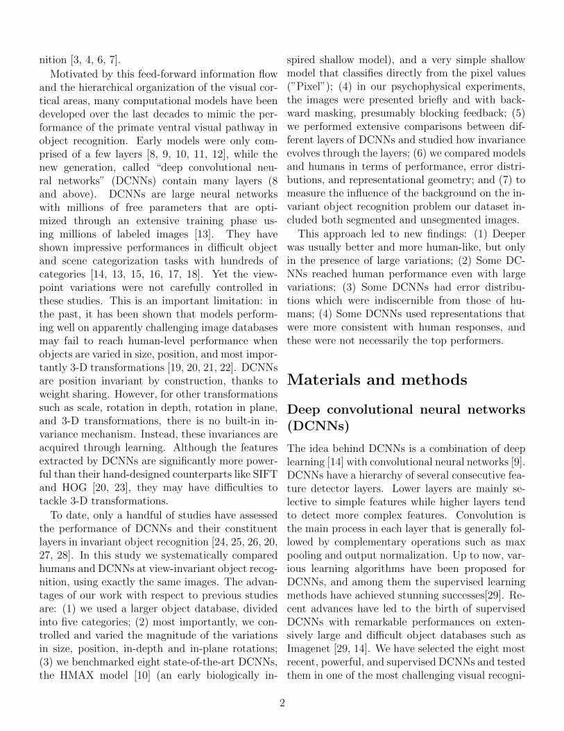
Figure 2: Classification accuracy of models and humans in mul-ticlass invariant object categorization task across seven levelsof object variations. A. Accuracies when objects were presented onuniform backgrounds. Each colored curve shows the accuracy of onemodel (specified in the legend). The gray curve indicates human cat-egorization accuracy across seven levels. All models were well abovechance level (20%). The right panel shows the accuracies of both mod-els and humans at the last level of variations (level seven; specified withpale, red rectangular), in ascending order. Level seven is consideredthe most difficult level as the variations are high at this level, makingthe categorization difficult for models and human. The color-codedmatrix, at the top-right of the bar plot, exhibits the p-values for allpairwise comparisons between human and models computed using theWilcoxon rank sum tests. For example, the accuracy of the Hybrid-CNN was compared to the human and all other models and the pair-wise comparison provides us with a p-value for each comparison. Bluepoints indicate that the accuracy difference is significant while graypoints show insignificant differences. Numbers, written around the p-value matrix, correspond to models (H stands for human). Accuraciesare reported as the average and standard deviation of 15 random, inde-pendent runs. B. Accuracies when objects were presented on randomlyselected natural backgrounds.
Results
We tested the DCNNs in our invariant object cat-egorization task including five object categories,seven variation levels, and two background condi-tions (see Materials and methods). The categoriza-tion accuracy of these models were compared withthose of human subjects, performing rapid invari-ant object categorization tasks on the same images.For each model, variation level, and backgroundcondition, we randomly selected 300 training im-ages and 150 testing ones per object category fromthe corresponding image dataset. The accuracywas then calculated over 15 random independentruns and the average and standard deviation werereported. We also analyzed the error distributionsof all models and compared them to those of hu-mans. Finally, we compared the representationalgeometry of models and humans, as a function ofthe variation levels.
DCNNs achieved human-level accu-racy
We compared the classification accuracy of the fi-nal layer of all models (DCNNs, and HMAX repre-sentation) with those of human subjects doing theinvariant object categorization tasks in all variationlevels and background conditions. Figure 2A showsthat almost all DCNNs achieved human-level accu-racy across all levels when objects had a uniformgray background. The accuracies of DCNNs areeven better than humans at low (levels 1 to 3) andintermediate (levels 4 and 5) variation levels. Thismight be due to inevitable motor errors that hu-mans made during the psychophysical experiment,meaning that subjects might have perceived theimage but pressed a wrong key. Also, it can beseen that the accuracies of humans and almost allDCNNs are virtually flat across all variation lev-els which means they are able to invariantly clas-sify objects with uniform background. Surprisingly,the accuracy of Overfeat is far below the human-level accuracy, even worse than the HMAX model.This might be due to the structure and the numberof features extracted by the Overfeat model whichleads to a more complex feature space with high
8

redundancy.We compared the accuracy of humans and mod-
els at the most difficult level (7). There is no signif-icant difference between the accuracies of CNN-S,CNN-M, Zeiler and Fergus, and human at this vari-ation level (Fig. 2A, bar plot; Also, see pairwisecomparisons shown using a p-value matrix com-puted by the Wilcoxon rank sum test). CNN-S isthe best model.
When we presented object images superimposedon natural backgrounds, the accuracies decreasedfor both humans and models. Figure 2B illustratesthat only three DCNNs (CNN-F, CNN-M, CNN-S) performed close to human. The accuracy ofthe HMAX model dropped down just above chancelevel (i.e., 20%) at the seventh variation level. In-terestingly, the accuracy of Overfeat remained al-most constant either in objects on uniform or natu-ral backgrounds, suggesting that this model is moresuitable for tasks with unsegmented images. Simi-larly, we compared the accuracies at the most diffi-cult level (level 7) when objects had natural back-grounds. Again, there is no significant differencebetween the accuracies of CNN-S, CNN-M, and hu-mans (see the p-value matrix computed using theWilcoxon rank sum test for all possible pairwisecomparisons). However, the accuracy of humansubjects is significantly above the HMAX modeland other DCNNs (i.e., CNN-F, Zeiler and Fergus,Krizhevsky, Hybrid-CNN, and Overfeat).
How accuracy evolves across layers inDCNNs
DCNNs have a hierarchical structure of differentprocessing stages in which each layer extracts alarge pool of features (e.g., > 4000 features at toplayers). Therefore, the computational load of suchmodels is very high. This raises important ques-tions: what is the contribution of each layer to thefinal accuracy? and how does the accuracy evolveacross the layers?
We addressed these questions by calculating theaccuracy of each layer of the models across all varia-tion levels. This provides us with the contributionof each layer to the final accuracy. Figure 3A-Hshows the accuracies of all layers and models when
objects had uniform gray background. The accura-cies of the Pixel representation (dashed, dark pur-ple curve) and human (gray curve) are also shownon each plot.
Overall, the accuracies significantly evolvedacross layers of DCNNs. Moreover, almost all lay-ers of the models (except Overfeat), even Pixel rep-resentation, achieved perfect accuracies at low vari-ation levels (i.e., levels 1 and 2), suggesting thatthis task is very simple when objects had smallvariations and uniform gray background. Look-ing at the intermediate and difficult variation levelsshows that the accuracies tend to increase as we goup across the layers. However, the trend is differ-ent between layers and models. For example, layers2, 3, and 4 in three DCNNs (Krizhevsky, Hybrid-CNN, Zeiler and Fergus) have very similar accu-racies across the variation levels (Fig. 3A, B, andG). Similar results can be seen for these models inlayers 5, 6, and 7 (Fig. 3A, B, and G). In contrast,there is a high increase in accuracies from layer 1 to4 for CNN-F, CNN-M, and CNN-S, while the threelast layers have similar accuracies. There is also agradual increase in the accuracy of Overfeat fromlayer 2 to 5 (with the similar accuracy for layers 6,7, and 8); however, there is a considerable decreaseat the output layer (Fig. 3C). Moreover, the over-all accuracy of Overfeat is low compared to humansand other models as previously seen in Fig. 2.
Interestingly, the accuracy of HMAX, as a shal-low model, is far below the accuracies of DCNNs(C2b is the best performing layer). This showsthe important role of supervised deep learning inachieving high classification accuracy. As expected,the accuracy of Pixel representation exponentiallydecreased down to 30% at level seven, confirmingthe fact that invariant object recognition requiresmulti-layered architectures (note that the chancelevel accuracy is 20%). We note, however, thatPixel performs very well with no viewpoint varia-tions (level 1).
We also compared the accuracies of all layersof the models with those of humans. Color-codedpoints at the top of each plot in Fig. 3 indicate thep-values of the Wilcoxon rank sum test. The aver-age accuracy of each layer across all variation levelsis shown on the pink area at the right side of each
9

1 2 3 4 5 6 730
40
50
60
70
80
90
100
Ave. of Levels
s. n.s.
Variation Levels
Ac
cu
rac
y (
%)
Krizhevsky et al. 2012
Human
Layer
7
Pixel
1 2 3 4 5 6 730
40
50
60
70
80
90
100
Ave. of Levels
s. n.s.
Variation Levels
Ac
cu
rac
y (
%)
−CNN 2014
Human
Layer
7
Pixel
Ave. of Levels
s. n.s.
Variation Levels
Ac
cu
rac
y (
%)
OverFeat 2014
1 2 3 4 5 6 730
40
50
60
70
80
90
100
Ave. of Levels
s. n.s.
Variation Levels
Ac
cu
rac
y (
%)
CNN−F. 2014
Human
Layer
7
Pixel
1 2 3 4 5 6 730
40
50
60
70
80
90
100
Ave. of Levels
s. n.s.
Variation Levels
Ac
cu
rac
y (
%)
CNN−M. 2014
Human
Layer
7
Pixel
1 2 3 4 5 6 730
40
50
60
70
80
90
100
Ave. of Levels
s. n.s.
Variation Levels
Ac
cu
rac
y (
%)
CNN−S 2014
Human
Layer
7
Pixel
1 2 3 4 5 6 730
40
50
60
70
80
90
100
Ave. of Levels
s. n.s.
Variation Levels
Ac
cu
rac
y (
%)
Zeiler and Fergus 2013
Human
Layer
7
Pixel
1 2 3 4 5 6 730
40
50
60
70
80
90
100
Ave. of Levels
s. n.s.
Variation Levels
Ac
cu
rac
y (
%)
HMAX 2007
Human
C2
C2b
C3
Pixel
1 2 3 4 5 6 7 8 950
60
70
80
90
100
Layers
Av
e.
Ac
cu
rac
y (
%)
Krizhevsky et al. 2012
CNN−F 2014
CNN−M 2014
CNN−S 2014
−CNN 2014
Zeiler and Fergus 2013
OverFeat 2014
HMAX 2007
Figure 3: Classification accuracy of models (for all layers separately) and humans in multiclass invariant object categorizationtask across seven levels of object variations, when objects had uniform backgrounds. A. Accuracy of Krizhevsky et. al. 2012 acrossall layers and levels. Mean accuracies and s.e.m. are reported using 15 random, independent runs. Each colored curve shows the accuracy ofone layer of the model (specified on the bottom-left legend). The accuracy of Pixel representation is depicted using a dashed, dark purple curve.The gray curve indicates human categorization accuracy across seven levels. The chance level is 20%; no layer hit the chance level for this task(note that the accuracy of Pixel representation dropped down to 10% above chance at level seven). The color-coded points at the top of theplot indicate whether there is a significant difference between the accuracy of humans and model layers (computed using the Wilcoxon ranksum test). Each color refers to a p-value, specified on the top-right (∗: p < 0.05, ∗∗: p < 0.01, ∗ ∗ ∗: p < 0.001, ∗ ∗ ∗∗: p < 0.0001). Coloredcircles on the pink area, show the average accuracy of each layer, across all variation levels (one value for each layer and all levels), with thesame color code as curves. The horizontal lines, depicted underneath the circles, indicate whether the difference between human accuracy (graycircle) and layers of the model is significant (computed using the Wilcoxon rank sum test; black line: significant, white line: insignificant). B-H.Accuracies of Hybrid-CNN, Overfeat, CNN-F, CNN-M, CNN-S, Zeiler and Fergus, and HMAX model, respectively. I. The average accuracyacross all levels for each layer of each model (again error bars are s.e.m.). Each curve corresponds to a model. This simply summarizes theaccuracies, depicted in the pink areas. The shaded area shows the average baseline accuracy (pale-purple, Pixel representation) and humanaccuracy (gray) across all levels.
plot, summarizing the contribution of each layerto final accuracy independently of variation levels.Horizontal lines on the pink area show whether theaverage accuracy of each layer is significantly differ-
ent from those of humans (black: significant; white:insignificant). Furthermore, Fig. 3I summarizes theresults depicted on the pink areas, confirming thatthe last three layers in DCNNs (except Overfeat)
10

s. n.s.
Krizhevsky et al. 2012
s. n.s.
OverFeat 2014
s. n.s.
CNN−F 2014
s. n.s.
CNN−M 2014
s. n.s.
Zeiler and Fergus 2013
s. n.s.
HMAX 2007
s. n.s.
−CNN 2014
s. n.s.
CNN−S 2014
1 2 3 4 5 6 7 8 9
30
40
50
60
70
80
90
100
Layers
Av
e.
Ac
cu
rac
y (
%)
Figure 4: Classification accuracy of models (for all layers separately) and human in multiclass invariant object categorizationtask across seven levels of object variations, when objects had natural backgrounds. A-H. Accuracies of Krizhevsky et. al.,Hybrid-CNN, Overfeat, CNN-F, CNN-M, CNN-S, Zeiler and Fergus, and HMAX model across all layers and variation levels, respectively. I.The average accuracy across all levels for each layer of each model (again error bars are s.e.m.). Details of diagrams are explained in the captionof Fig. 3
have similar accuracies.
We also tested the models on objects with nat-ural backgrounds to see whether the contributionsof similarly performing layers change in more chal-lenging tasks. Not surprisingly, the accuracy of hu-man subjects dropped by 10% at low variation level(level 1), and down to 25% at high variation level(level 7) with respect to the uniform backgroundcase (Fig. 4, gray curve). Not surprisingly, the Pixelrepresentation shows an exponential decline in the
accuracy across the levels, with the chance accuracyat level seven (Fig. 4, dashed dark purple curve).Similar to Fig. 3, all DCNNs, excluding Overfeat,achieved close to human-level accuracy at low vari-ation levels (levels 1, 2, and 3). Interestingly, thePixel representation performed better than mostmodels at level one, suggesting that object catego-rization at low variation level can be done withoutelaborate feature extraction methods (note that wehad only five object categories, therefore, this can
11

1 2 3 4 5 6 7 8 920
30
40
50
60
70
80
90
100
Layers
Accu
racy (
%)
1 2 3 4 5 6 7 8 920
30
40
50
60
70
80
90
100
Layers
Accu
racy (
%)
Krizhevsky et al. 2012
CNN−F 2014
CNN−M 2014
CNN−S 2014
−CNN 2014
Zeiler and Fergus 2013
OverFeat 2014
HMAX 2007
1 2 3 4 5 6 7 8 920
30
40
50
60
70
80
90
100
Layers
Accu
racy (
%)
1 2 3 4 5 6 7 8 920
30
40
50
60
70
80
90
100
Layers
Accu
racy (
%)
1 2 3 4 5 6 7 8 920
30
40
50
60
70
80
90
100
Layers
Accu
racy (
%)
1 2 3 4 5 6 7 8 920
30
40
50
60
70
80
90
100
Layers
Accu
racy (
%)
Figure 5: Classification accuracy at easy (level 1), intermediate (level 4) and difficult (level 7) levels for different layers of themodels. A-C. Accuracy for different layers at easy (A), intermediate (B) and difficult (C) levels when objects had uniform backgrounds. Eachcurve represents the accuracy of a model. The shaded areas show the accuracy of the Pixel representation (pale purple) and human (gray).Error bars are standard deviation. D-F. Idem when objects had natural backgrounds.
be different with more categories).
The severe drop in the accuracy of the HMAXmodel with respect to the uniform background ex-periment reflects the difficulty of this model to copewith distractors in natural backgrounds. For bothbackground conditions, the C2b layer has higheraccuracy than C3 layer and can better tolerate ob-ject variations. The main reason why HMAX isnot performing as well as DCNNs is probably thelack of a purposive learning rule [45, 21]. HMAXrandomly extracts a large number of visual features(image crops) which could be highly redundant, un-informative, and even misleading [46]. The issue ofinappropriate features becomes more evident whenthe background is clutter.
Another noticeable fact about DCNNs in the nat-ural background experiment is the superiority ofthe last convolutional layers with respect to thefully connected layers; for example, the accuracyof the fifth layer in the Krizhevsky model is higherthan the seventh layer’s. One possible reason forthe low accuracies in the final layers of DCNNs isthat the fully connected layers are designed to per-
form classification themselves, and not to provideinput for a SVM classifier. Besides, the fully con-nected layers were optimized for Imagenet classifi-cation, but not for our dataset. A last reason couldbe that the convolutional layers have more featuresthan the fully connected layers.
Given the accuracies of all layers, it can be seenthat the accuracies evolved across the layers. How-ever, similar to Fig. 3, layers 2, 3, and 4 of Krizh-esvky, Zeiler and Fergus, and Hybrid-CNN con-tribute almost equally to the final accuracy. Again,CNN-F, CNN-M, and CNN-S showed a differenttrend in terms of the contribution of each layer tothe final accuracy. Moreover, as shown in Fig. 4D-F, only these three models achieved human-levelaccuracy at difficult levels (levels 6 and 7). The ac-curacies of other DCNNs, however, are significantlylower than humans at these levels (see the color-coded points in Fig. 4A-C, G which indicate the p-values computed by the Wilcoxon rank sum tests).We summarized the average accuracies across alllevels for each layer of the models, shown as color-coded circles with error bars on the pink areas next
12

Figure 6: Confusion matrices for multiclass invariant object categorization task. A. Each color-coded matrix shows the confusionmatrix of a model when categorizing different object categories (specified in the first matrix at the top-left corner), when images had uniformbackgrounds. Each row corresponds to a model. Last row shows human confusion matrix. Each column indicates a particular level of variation(levels 1 to 7). Models’ name is depicted at the right end. B. Idem with natural backgrounds. The color bar at the top-right shows thepercentage of the labels assigned to each category, The chance level indicated with an arrow. Confusion matrices were calculated only for thelast layers of the models.
to each plot. In most cases, layer 5 (the last con-volutional layer - layer 6 in Overfeat) has the high-est accuracy among layers. This is summarized inFig. 4I, which is actually the summary of resultsshown on pink areas. Figure 4I also confirms thatonly CNN-F, CNN-M, and CNN-S achieve human-level accuracy.
We further compared the accuracies of all layersof the models with humans at the easy (level 1), in-termediate (level 4) and difficult (level 7) variationlevels to see how each layer performs the task asthe level of variations increases. Figure 5A-C showthe accuracies for the uniform background condi-tion. The easy level is not very informative be-cause of a ceiling effect: all models (but Overfeat)reach 100% accuracy. At the intermediate level, allDCNNs (except Overfeat) reached the human-levelaccuracy from layer 4 upwards (Fig. 5A), suggest-ing that even with intermediate level of variation,DCNNs have remarkable accuracies (note that ob-
jects had uniform background). This is clearly nottrue for the HMAX and Overfeat networks. How-ever, when models were fed with images from themost difficult level, only the last layers (layers 5, 6,and 7) achieved human-level accuracy (see Fig. 5B).Notably the last three layers have almost similaraccuracies.
When objects had natural backgrounds, some-what surprisingly the accuracies of all DCNNs (butOverfeat) is maximal with layer 2, and drops forsubsequent layers. This shows that deeper is notalways better. The fact that the Pixel representa-tion performs well at this level confirms this find-ing. At the intermediate level, the picture is differ-ent: only the last three layers of DCNNs, excludingOverfeat, reach human-level accuracy (see Fig. 5E).Finally, at the seventh variation level, Figure 5Fshows that only three DCNNs reach human perfor-mance: CNN-F, CNN-M, and CNN-S.
In summary, the above results, taken together,
13

illustrate that some DCNNs are as accurate as hu-mans, even at the highest variation levels.
Do DCNNs and humans make similarerrors?
The accuracies reported in the previous sectiononly represent the ratio of correct responses. In-deed, they did not reflect whether models and hu-mans made similar misclassifications. To do a moreprecise and category-based comparison between therecognition accuracies of humans and models, wecomputed the confusion matrices for each variationlevel. Figure 6 provides the confusion matrices forhumans and the last layers of all models for bothuniform (see Fig. 6A) and natural (see Fig. 6B)backgrounds, and for each variation level.
Despite a very short presentation time in thebehavioral experiment, humans performed remark-ably well at categorizing five object classes, eitherwhen object had uniform (Fig. 6A, last row) ornatural (Fig. 6B, last row) backgrounds, with min-imum misclassifications across different categoriesand levels. It is, however, important to point outthat the majority of human errors corresponded toship - airplane confusions. This was probably dueto the shape similarity among these objects (e.g.,both categories usually have bodies, sails, wings,etc.).
Figure 6 demonstrates that the HMAX modeland Pixel representation misclassified almost allcategories at high variation levels. With naturalbackgrounds, they uniformly assigned input imagesinto different classes. Conversely, DCNNs show fewclassification errors across different categories andlevels, though the distribution of errors is differ-ent from one model to another. For example, themajority of recognition errors made by Krizehvsy,Zeiler and Fergus, and Hybrid-CNN belonged tocar and motorcycle classes, while animal and air-plane classes were mostly misclassified by CNN-F, CNN-M, and CNN-S. Finally, Overfeat showsevenly-distributed errors across categories, confirm-ing its low accuracy.
We also examined whether models’ decisions aresimilar to those of humans. To this end, we com-puted the similarity between the humans’ confusion
matrices and those of the models. An importantpoint is to factor out the impacts of the mean ac-curacies (of humans and models) on the similaritymeasure, to only take the error distributions intoaccount. Therefore, for each confusion matrix, wefirst excluded the diagonal terms and arranged theremaining elements in a vector and normalized itby its L2 norm. Then, the similarity between twoconfusion matrices is computed using the Euclideandistance between their corresponding vectors sub-tracted from one (here we call it as 1 - Norm. Eu-clidean distance). In this way, we are just compar-ing the error distributions of humans and modelsindependent of their accuracies. Figure 7 providesthe similarities between models and humans acrossall layers and levels when objects had uniform back-ground. Almost all models, including the Pixel rep-resentation, show the maximum possible similarityat low variation levels (levels 1 and 2). However,the similarity of Pixel representation exponentiallydecreases from level 2 upwards. Overall, the high-est layers of DCNNs (except Overfeat) are moresimilar to humans’ decisions. This point is alsoshown in Figure 7I, which represents the averagesimilarities across all variation levels (each curvecorresponds to one model). Note that due to thehigh recognition accuracies in uniform backgroundcondition, this level of similarity was predictable.
The similarity between models’ and humans’ er-rors, however, decreases in the case of images withnatural backgrounds. The HMAX model had thelowest similiarity with human (see Fig. 8). Al-though DCNNs have reached human-level accuracy,their decisions and distribution of errors are dif-ferent from human’s. Interestingly, the Overfeathas almost a constant similarity across layers andlevels. Comparing the similarities across DCNNsshows that CNN-F, CNN-M, and CNN-S have thehighest similarities to humans, which is also re-flected in Fig. 8I.
To summarize our results so far: the best DCNNscan reach human performance even at the highestvariation level, but their error distributions are dif-ferent to the average human one (similarity < 1 onFig. 8). However, one needs a reference here, be-cause humans also differ between each other. Arethese difference between humans smaller than dif-
14

1 2 3 4 5 6 7
0.2
0.4
0.6
0.8
1
Variation Levels
1−
No
rm.
Eu
cli
de
an
Dis
tan
ce
Variation Levels
1 2 3 4 5 6 7 8 90.4
0.6
0.8
1
Layers
1−
Av
e.
Eu
cli
de
an
Dis
tan
ce
C2b
C3
Pixel
C
1 2 3 4 5 6 7
0.2
0.4
0.6
0.8
1
Variation Levels
1−
No
rm.
Eu
cli
de
an
Dis
tan
ce
1 2 3 4 5 6 7
0.2
0.4
0.6
0.8
1
Variation Levels
1−
No
rm.
Eu
cli
de
an
Dis
tan
ce
1 2 3 4 5 6 7
0.2
0.4
0.6
0.8
1
1−
No
rm.
Eu
cli
de
an
Dis
tan
ce
1 2 3 4 5 6 7
0.2
0.4
0.6
0.8
1
Variation Levels
1−
No
rm.
Eu
cli
de
an
Dis
tan
ce
1 2 3 4 5 6 7
0.2
0.4
0.6
0.8
1
Variation Levels
1−
No
rm.
Eu
cli
de
an
Dis
tan
ce
1 2 3 4 5 6 7
0.2
0.4
0.6
0.8
1
1−
No
rm.
Eu
cli
de
an
Dis
tan
ce
1 2 3 4 5 6 7
0.2
0.4
0.6
0.8
1
Variation Levels
1−
No
rm.
Eu
cli
de
an
Dis
tan
ce
Figure 7: Similarity between models’ and humans’ confusion matrices when images had uniform backgrounds. A. Similaritybetween Krizhevsky et al. 2012 confusion matrices and that of humans (measured as 1-normalized Euclidean distance). Each curve shows thesimilarity between human confusion matrix and one layer of Krizhevsky et al. 2012 (specified on the right legend), across different levels ofvariations. The similarity between the confusion matrix of the Pixel representation and humans is shown using a dark purple, dashed line. B-H.Idem for the Hybrid-CNN, Overfeat, CNN-F, CNN-M, CNN-S, Zeiler and Fergus, and HMAX models, respectively. I. The average similarityacross all levels for each layer of each model (error bars are s.e.m.). Each curve corresponds to one model.
ferences between humans and DCNNs? To investi-gate this issue, we used the multidimensional scal-ing (MDS) method to visualize the distances (i.e.,similarities) between the confusion matrices of hu-mans and models (last layer) in 2-D maps (see Fig-ure 9). Each map corresponds to a certain variationlevel and background condition.
In the uniform background condition, humanshave small inter-subject distances. As we movefrom low to high variations, the distance betweenDCNNs and humans becomes greater. In high vari-ation levels, the Overfeat, HMAX, and Pixel mod-els are very far from the human subjects as well asfrom the other DCNNs. The other models remainindiscernible from humans.
In the natural background condition, the hu-man between-subject distances are relatively higher
than in the uniform condition. As the level of varia-tions increases, the models tend to get further awayfrom the human subjects. But the CNN-F, CNN-M, and CNN-S are difficult, if not impossible, todiscern from humans.
So far, we have analyzed the accuracies and errordistributions of models and humans, when featureswere used by a SVM classifier. However, such anal-yses do not inform us about the internal represen-tational geometry of models and their similaritiesto those of humans. It is very important to investi-gate how different categories are represented in thefeature space.
15

1 2 3 4 5 6 70
0.2
0.4
0.6
0.8
1
Variation Levels
1−
No
rm.
Eu
cli
de
an
Dis
tan
ce
1 2 3 4 5 6 7 8 90
0.2
0.4
0.6
0.8
1
Layers
1−
Av
e.
Eu
cli
de
an
Dis
tan
ce
Variation Levels
1 2 3 4 5 6 70
0.2
0.4
0.6
0.8
1
Variation Levels
1−
No
rm.
Eu
cli
de
an
Dis
tan
ce
1 2 3 4 5 6 70
0.2
0.4
0.6
0.8
1
Variation Levels
1−
No
rm.
Eu
cli
de
an
Dis
tan
ce
1 2 3 4 5 6 70
0.2
0.4
0.6
0.8
1
1−
No
rm.
Eu
cli
de
an
Dis
tan
ce
1 2 3 4 5 6 70
0.2
0.4
0.6
0.8
1
Variation Levels
1−
No
rm.
Eu
cli
de
an
Dis
tan
ce
1 2 3 4 5 6 70
0.2
0.4
0.6
0.8
1
Variation Levels
1−
No
rm.
Eu
cli
de
an
Dis
tan
ce
1 2 3 4 5 6 7
0
0.2
0.4
0.6
0.8
1
Variation Levels
1−
No
rm.
Eu
cli
de
an
Dis
tan
ce
1 2 3 4 5 6 70
0.2
0.4
0.6
0.8
1
Variation Levels
1−
No
rm.
Eu
cli
de
an
Dis
tan
ce
Figure 8: Similarity between models’ and humans’ confusion matrices, when object images had natural backgrounds. A-H.Similarities between the confusion matrices of Krizhevsky, Hybrid-CNN, Overfeat, CNN-F, CNN-M, CNN-S, Zeiler and Fergus, HMAX modeland that of humans. Figure conventions are identical to Fig. 7. I. The average similarity across all levels for each layer of each model (errorbars are s.e.m.). Each curve corresponds to a model.
Representational geometry of modelsand human
Representational similarity analysis has become apopular tool to study the internal representationof models [20, 47, 27, 48] in response to differentobject categories. The representational geometriesof models can then be compared with neural re-sponses independently of the recording modality(e.g. fMRI [48, 20], cell recording [49, 47, 27], be-havior [50, 51, 52, 19], and MEG [53]), showing towhat degree each model resembles the brain rep-resentations. Here, we calculated representationaldissimilarity matrices (RDM) for models and hu-mans [44]. We then compared the RDMs of hu-mans and each model and quantified the similaritybetween these two. Model RDMs were calculatedbased on pairwise correlation between the featurevectors of two images (see Materials and methods).
To calculate the human RDM, we used their behav-ioral scores recorded in the psychophysical experi-ment (see Materials and methods as well as [19]).
Figure 10 represents the RDMs for models andhuman across different levels of variation bothfor objects on uniform (Fig. 10A) and natural(Fig. 10B) backgrounds. Note that these RDMsare calculated from the object representations inthe last layers of the models. For better visualiza-tion, we show only 20 images from each category;therefore, the size of RDMs is 100 × 100 (reportedRDMs were averaged over six random runs).
As expected, human RDM clearly representseach object category, with minimum intra-class dis-similarity and maximum inter-class dissimilarity,across all variation levels (last row in Fig. 10A andFig. 10B for uniform and natural backgrounds, re-spectively). However, both HMAX and Pixel rep-resentation show a random pattern in their RDMs
16

Figure 9: The distances between models and humans visualized using the multidimensional scaling (MDS) method. distancesbetween models and humans when images had uniform (A) and natural backgrounds (B). Light gray circles show the position of each humansubjects and larger black circle shows the average of all subjects. Color circles represent models.
when objects had natural backgrounds (Fig. 10B,rows 8 and 9), suggesting that such low and in-termediate visual features are unable to invariantlyrepresent different object categories. The situationis slightly better when object had uniform back-ground (Fig. 10A, rows 8 and 9). In this case, thereis some categorical information, mostly across lowvariation levels (levels 1 to 3, and 4 to some extent),for animal, motorcycle, and airplane images. Suchinformation is attenuated at intermediate and highvariation levels.
In contrast, DCNNs demonstrate clear categori-cal information for different objects across almost
all levels, for both background conditions. Cate-gorical information is more evident when objectshad uniform background, even at high variationlevels, while this information almost disappears atintermediate levels when object had natural back-grounds. In addition, Overfeat did not clearly rep-resent different object categories. The Overfeatmodel is one of the most powerful DCNNs withhigh accuracy on the Imagenet database, but itseems that the features are not suitable for our in-variant object recognition task. It uses no fewerthan 230400 features! This might be one reason forpoor representational power: it probably leads to a
17

Figure 10: Representational Dissimilarity Matrices (RDM) for models and humans. RDMs for humans and models when imageshad uniform (A) and natural (B) backgrounds. Each element in a matrix shows the pairwise dissimilarities between the internal representationsof the two images (measured as 1− Spearman’s rank correlation). Each row of RDMs corresponds to a model (specified on the right) and eachcolumn corresponds to a particular level of variation (from level 1 to 7). Last row illustrates the human RDMs, calculated from the behavioralresponses. The color bar on the top-right corner shows the degree of dissimilarity. For the sake of visualization, we only included 20 imagesfrom each category, leading to 100 × 100 matrices. Model RDMs were calculated for the last layer of each model.
nested and complex object representation. Besides,this high number of features may also explain thepoor classification performance we obtained, due tooverfitting.
Based on visual inspection, it seems that someDCNNs are better at representing some specificcategories. For example, Krizhevsky, Hybrid-CNN,Zeiler and Fergus could better represent animal, carand airplane classes (lower within-class dissimilar-ity for these categories), while ship and motorcycleclasses are better represented by CNN-F, CNN-M,and CNN-S. Interestingly, this has been reflectedon the confusion matrix analysis, suggesting thatcombining and remixing of features from these DC-NNs could result in a more robust invariant objectrepresentation [20].
To quantify the similarity between models’ andhumans’ RDMs, we calculated the correlation be-tween them across all layers and levels (measured asKendall τa rank correlation). Each panel in Fig. 11
and Fig. 12 represents the correlation between mod-els’ and humans’ RDMs across all layers and vari-ation levels (each color-coded curve corresponds toone layer) when object had uniform and naturalbackgrounds, respectively. Overall, as shown inthese figures, the correlation coefficients are high atlow variation levels , but decrease at higher levels.Moreover, correlations are not significant at verydifficult levels, as specified with color-coded pointson the top of each plot (blue point: significant, graypoint: insignificant).
Interestingly, comparing the cases of uniform(Fig. 11) and natural (Fig. 12) backgrounds indi-cates that the maximum correlation (∼ 0.3 at level1) did not change a lot. However, for the uniformbackground condition, the correlation across otherlevels increased to some extent. Besides, it can alsobe seen that the correlations of the HMAX modeland Pixel representation are higher and more sig-nificant than with natural backgrounds (Fig. 11H
18

Variation Levels Variation Levels Variation Levels
Variation Levels Variation Levels Variation Levels
Variation Levels Variation Levels
Co
rre
lati
on
Wit
h H
um
an
(Ke
nd
all
sτ
a)
Co
rre
lati
on
Wit
h H
um
an
(Ke
nd
all
sτ
a)
Co
rre
lati
on
Wit
h H
um
an
(Ke
nd
all
sτ
a)
1 2 3 4 5 6 7 8 9
0
0.05
0.1
0.15
0.2
0.25
Layers
Av
e.
Co
rre
lati
on
Figure 11: Correlation between humans’ and models’ RDMs, across different layers and levels, when objects had uniformbackgrounds. A. Correlation between human RDM and Krizhevsky et. al. 2012 RDM (Kendall τa rank correlation), across different layersand levels of variations. Each color-coded curve shows the correlation of one layer of the model (specified on the right legend) with thecorresponding human RDM. The correlation of Pixel representation with human RDM is depicted using a dashed, dark purple curve. Thecolor-coded points on the top of the plots indicate whether the correlation is significant. Blue points indicate significant correlation while graypoints show insignificant correlation. Correlation values are the average over 10,000 bootstrap resamples. Error bars are the standard deviation.B-H. Idem for Hybrid-CNN, Overfeat, CNN-F, CNN-M, CNN-S, Zeiler and Fergus, and HMAX, respectively. I. The average correlation acrossall levels for each layer of each model (error bars are STD). Each curve corresponds to one model. The shaded area shows the average correlationfor the Pixel representation across all levels. All correlation values were calculated using the RSA toolbox (Nili et al., 2014).
and Fig. 12H). Note that the correlation values ofthe first layer of almost all DCNNs (but Zeiler andFergus) are similar to those of Pixel representa-tion, suggesting that in the absence of viewpointvariations, very simple features (i.e., gray values ofpixels) can achieve acceptable accuracy and corre-lation. This means that DCNNs are built to per-form more complex recognition tasks, as it has beenshown in several studies.
Not surprisingly, in the case of natural back-
ground, the correlation between Pixel and humanRDMs are very low and almost insignificant at alllevels (Fig. 12 dashed dark purple line copied onall panels). Similarly, the HMAX model shows avery low and insignificant correlation across all lay-ers and levels. We also expected a low correlationfor the Overfeat model, as shown in Fig. 12C. In-terestingly, the correlation increases as images areprocessed across consecutive layers in DCNNs, withlower correlations at early layers and higher corre-
19

1 2 3 4 5 6 7
−0.05
0
0.05
0.1
0.15
0.2
0.25
0.3
Variation Levels
Co
rre
lati
on
Wit
h H
um
an
(Ke
nd
all
sτ
a)
1 2 3 4 5 6 7
−0.05
0
0.05
0.1
0.15
0.2
0.25
0.3
Variation Levels
1 2 3 4 5 6 7
−0.05
0
0.05
0.1
0.15
0.2
0.25
0.3
Variation Levels
1 2 3 4 5 6 7
−0.05
0
0.05
0.1
0.15
0.2
0.25
0.3
Variation Levels
1 2 3 4 5 6 7
−0.05
0
0.05
0.1
0.15
0.2
0.25
0.3
Variation Levels
1 2 3 4 5 6 7
−0.05
0
0.05
0.1
0.15
0.2
0.25
0.3
Variation Levels
Av
e.
Co
rre
lati
on
Co
rre
lati
on
Wit
h H
um
an
(Ke
nd
all
sτ
a)
1 2 3 4 5 6 7
−0.05
0
0.05
0.1
0.15
0.2
0.25
0.3
Variation Levels
C2
C2b
C3
Pixel
1 2 3 4 5 6 7
−0.05
0
0.05
0.1
0.15
0.2
0.25
0.3
Variation Levels
Co
rre
lati
on
Wit
h H
um
an
(Ke
nd
all
sτ
a)
1 2 3 4 5 6 7 8 9
0
0.05
0.1
0.15
0.2
0.25
Figure 12: Correlation between humans’ and models’ RDMs, across different layers and levels, when objects had naturalbackgrounds. A-H. Correlation between humans’ RDM and the one of KirZhevsky, Hybrid-CNN, Overfeat, CNN-F, CNN-M, CNN-S, Zeilerand Fergus, and HMAX, across all layers and levels. Figure conventions are identical to Fig. 11. I. The average correlation across all levels foreach layer of each model (error bars are STD).
lations at top layers (layer 5, 6, and 7). As for theaccuracy results, the correlations of fully connectedlayers of DCNNs are very similar to each other, sug-gesting that these layers do not greatly add to thefinal representation.
We summarized the correlation results in Fig. 11Iand Fig. 12I, by averaging the correlation coef-ficients across levels for every model layer. Itis shown that the correlations for DCNNs evolveacross layers, with low correlations at early lay-ers and high correlations at top layers. More-over, Fig. 11I shows that the correlation of theHMAX model (all the layers) with human fluctu-ates around the correlation of Pixel representation
(specified with shaded area).Note that although the correlation coefficients
are not very high (∼ 0.2), Zeiler and Fergus,Hybrid-CNN, and Krizhevsky models are the mosthuman-like. It is worth noting that the best mod-els in terms of performance, CNN-F, CNN-M, andCNN-S do not have the most human-like RDMs.Conversely, the model with the most human-likeRDM, Zeiler and Fergus, is not the best in termsof classification performance.
More research is needed to understand whythe Zeiler and Fergus’ RDM is significantly morehuman-like than those of other DCNNs. This find-ing is consistent with a previous study by Cadieu et
20
al.[27], in which the Zeiler and Fergus’ RDM wasfound be more similar to monkey IT RDM thanthose of the Krizhevsky and HMAX models.
We also computed the category separability in-dex for the internal representations of each modelby computing the ratio of within-category rela-tive to between-category dissimilarities (results arenot shown here).This experiment also confirms thatmodels with higher separability indexes do not nec-essarily perform better than other models. In fact,it is the actual positions of images of different cat-egories in the representational space which deter-mines the final accuracy of a model, not just themean inter- and intra-class distances.
A very deep network
In previous sections we studied different DCNNs,each having 8 or 9 layers with 5 or 6 convolu-tional layers, from various perspectives and com-pared them with the human feed-forward objectrecognition system. Here, we assess how exploitingmany more layers could affect the performance ofDCNNs. To this end, we used Very Deep CNN [32]that has no fewer than 19 layers (16 convolutionaland 3 fully connected layers). We extracted fea-tures of layers 9 to 18 from images with natu-ral backgrounds, to investigate if more layers inthe Very Deep CNN affects the final accuracy andhuman-likeness.
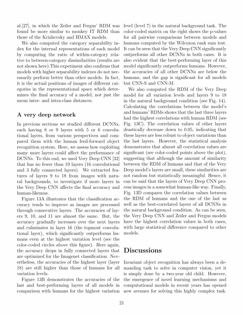
Figure 13A illustrates that the classification ac-curacy tends to improve as images are processedthrough consecutive layers. The accuracies of lay-ers 9, 10, and 11 are almost the same. But, theaccuracy gradually increases over the next layersand culminates in layer 16 (the topmost convolu-tional layer), which significantly outperforms hu-mans even at the highest variation level (see thecolor-coded circles above this figure). Here again,the accuracy drops in fully connected layers thatare optimized for the Imagenet classification. Nev-ertheless, the accuracies of the highest layer (layer18) are still higher than those of humans for allvariation levels.
Figure 13B demonstrates the accuracies of thelast and best-performing layers of all models incomparison with humans for the highest variation
level (level 7) in the natural background task. Thecolor-coded matrix on the right shows the p-valuesfor all pairwise comparisons between models andhumans computed by the Wilcoxon rank sum test.It can be seen that the Very Deep CNN significantlyoutperforms all other DCNNs in both cases. It isalso evident that the best-performing layer of thismodel significantly outperforms humans. However,the accuracies of all other DCNNs are below thehumans, and the gap is significant for all modelsbut CNN-S and CNN-M.
We also computed the RDM of the Very Deepmodel for all variation levels and layers 9 to 18in the natural background condition (see Fig. 14).Calculating the correlations between the model’sand humans’ RDMs shows that the last three layershad the highest correlations with human RDM (seeFig. 13C). The correlation values of other layersdrastically decrease down to 0.05, indicating thatthese layers are less robust to object variations thanthe last layers. However, the statistical analysisdemonstrates that almost all correlation values aresignificant (see color-coded points above the plot),suggesting that although the amount of similaritybetween the RDM of humans and that of the VeryDeep model’s layers are small, these similarities arenot random but statistically meaningful. Hence, itcan be said that the layers of Very Deep CNN pro-cess images in a somewhat human-like way. Finally,Fig. 13D compares the correlation values betweenthe RDM of humans and the one of the last aswell as the best-correlated layers of all DCNNs inthe natural background condition. As can be seen,the Very Deep CNN and Zeiler and Fergus modelshave the highest correlation values in both cases,with large statistical difference compared to othermodels.
Discussions
Invariant object recognition has always been a de-manding task to solve in computer vision, yet itis simply done by a two-year old child. However,the emergence of novel learning mechanisms andcomputational models in recent years has openednew avenues for solving this highly complex task.
21

1 2 3 4 5 6 720
30
40
50
60
70
80
90
100
Ave. of Levels
s. n.s.
Variation Levels
Ac
cu
rac
y (
%)
Very Deep 2014
Human
Layer 9
- 18
Pixel
20
30
40
50
60
70
80
Ac
cu
rac
yo
f
last
layer
(%)
91 2 3 4 5 6 7 8 9H
Ver
y D
eep
Models
9
1 2 3 4 5 6 7 8
20
30
40
50
60
70
80
Models
Ac
cu
rac
y(%
)
Ver
y D
eep
9
9
1 2 3 4 5 6 70
0.05
0.1
0.15
0.2
0.25
0.3
Variation Levels
Co
rre
lati
on
Wit
h H
um
an
(K
en
da
lls
τa)
Layer 9
- 18
Very Deep 2014
1 2 3 4 5 6 7 8 9
0
0.05
0.1
0.15
0.2
Models
Ver
y D
eep
1 2 3 4 5 6 7 8 90
0.05
0.1
0.15
0.2
Models
Ver
y D
eep
Co
rre
lati
on
Wit
h H
um
an
(K
en
da
lls
τa)
Figure 13: The accuracy and human-likeness of the Very Deep CNN with natural backgrounds. A. Classification accuracy of theVery Deep CNN (layers 9-18 ) and humans across the seven levels of object variations. Each colored curve shows the accuracy of one layer of themodel. The accuracy of the Pixel representation is depicted using a dashed, dark purple curve. The gray curve indicates human categorizationaccuracy across the seven levels. The color-coded points at the top of the plot indicate whether there is a significant difference between theaccuracy of humans and each layer of the model (Wilcoxon rank sum test). Each color refers to a p-value, specified on the top-right (∗: p < 0.05,∗∗: p < 0.01, ∗ ∗ ∗: p < 0.001, ∗ ∗ ∗∗: p < 0.0001). We plot the mean accuracies +/- STD over 15 runs. Colored circles with error bars, onthe pink area show the average accuracy of each layer across all variation levels (mean +/- STD). The horizontal lines underneath the circles,indicate whether the difference between human accuracy (gray circle) and each layer of the model is significant (Wilcoxon rank sum test; blackline: significant, white line: insignificant). B. Top: the accuracy comparison between the best-performing layer in each model and humans atthe last variation level (level 7). The color-coded matrix, on the right of the bar plot, shows the p-values for all pairwise comparisons betweenhumans and models (Wilcoxon rank sum test). Numbers, written around the p-value matrix, correspond to models (H stands for human).Bottom: idem with the last layers. C. Correlation between humans and the Very Deep CNN RDMs, across different layers (layers 9-18) andlevels. Each color-coded curve shows the correlation of one layer of the model with corresponding human RDM. The color-coded points at thetop of the plot indicate whether the correlation is significant (Blue: significant; Gray: insignificant). Correlation values are the average over10,000 bootstrap resamples +/- STD. D. Top: correlations between the most correlated layer in each model and humans at the last variationlevel (level 7). P-value matrix was calculated using similar approach to B. Bottom: idem with the last layers.
DCNNs have been shown to be a novel and pow-erful approach to tackle this problem [15, 54, 55,16, 56, 57, 58, 27, 59, 60]. These networks havedrawn scientists’ attention not only in vision sci-ences, but also in other fields of science (see [55]),as a powerful solution for many complex problems.
DCNNs are among the most powerful computingmodels inspired by computations performed in neu-ral circuits. To our interest, recent studies also con-firmed the abilities of DCNNs in object recognitionproblems (e.g. [15], [27], and [61]). Besides, severalstudies have tried to compare the responses of DC-
22

Figure 14: Representational Dissimilarity Matrices (RDM) of VeryDeep model (layers 9 to 18) for different levels of variation (from level1-7) in natural background condition. Each element in a matrix showsthe pairwise dissimilarities between the representations of two images(measured as 1-r, Spearman’s rank correlation. See Materials andMethods). The color bar at the top-right corner shows the degreeof dissimilarity. The size of each matrix is 100 × 100, with 20 imagesfrom each category. This was done for the sake of better visualization.
NNs and primate visual cortex in different objectrecognition tasks.
Khaligh-Razavi and Kriegeskorte [20] comparedthe representational geometry of neuronal re-sponses in human (fMRI data; see [48]) and mon-key IT cortex (cell recording; see [49]) with severalcomputational models, including one DCNN, on a96-image dataset. They showed that supervisedDCNNs can explain IT representation. However,firstly, their image database only contained frontalviews of objects with no viewpoint variation. Sec-ondly, the number and variety of images were verylow (only 96 images), compared to the wide varietyof complex images in natural environment. Finally,
images had a uniform gray background, which isvery different from natural vision. To overcomesuch issues, Cadieu et. al. [27] used a large imagedatabase, consisting of different categories, back-grounds, transformations, and compared the cate-gorization accuracy and representational geometryof three DCNNs and neural responses in IT andV4 of monkey. They showed that DCNNs closelyresemble the responses of IT neurons either in accu-racy or geometry [27, 47]. One issue in their studyis the long stimulus presentation time (100 ms),which might be too long to only account for feed-forward processing. Moreover, they included onlythree DCNNs in their study. In another attempt,Guclu et. al. [28] mapped different layers of aDCNN onto the human visual cortex. More specif-ically, they computed the representational similar-ities among different layers of a DCNN and thefMRI data from different areas in human visual cor-tex. Although these studies have shown the powerof several DCNNs in object recognition, advance-ments in developing new DCNNs are quick, whichrequires continuous assessments of recent DCNNsusing different techniques. Moreover, the ability ofDCNNs in tolerating object variations (mostly 3-Dvariations) had not been carefully evaluated before.
Here, we comprehensively tested eight best per-forming DCNNs, reported in the literature [15, 16,17, 18, 31, 32], in a very challenging vision task,namely invariant object recognition. This list ofDCNNs has shown remarkable accuracies in clas-sification of big and challenging image databasessuch as Imagenet, VOC 2007, and Caltech 205.Moreover, we compared the DCNNs with humansubjects performing the same task with the sameimages to investigate the extent to which DCNNsresemble humans.
DCNNs achieve human-level per-formance in rapid invariant objectrecognition task
Humans are very fast and accurate at categorizingobjects [5, 62, 63]. Numerous studies have inves-tigated this remarkable performance under ultra-rapid image presentation [64, 65, 66]. It is be-
23

lieved that rapid object categorization is mainlyperformed by the feed-forward information flowthrough the ventral visual pathway [67, 63]. Ex-perimental and theoretical evidence suggests thatfeed-forward processing is able to perform invari-ant object recognition [3, 4, 6, 7]. Here, we mea-sured human accuracy when categorizing five ob-ject categories in a rapid presentation paradigm.Objects varied in six dimensions and the task dif-ficulty was controlled using seven variation levels.Results showed that humans achieved high accu-racy across all levels (under 2- and 3-D variations)while objects were only presented for 25 ms.
Using the same image database, we also evalu-ated eight state-of-the-art DCNNs [15, 16, 17, 18,31], largely inspired by feed-forward processing ofvisual cortex. Results indicated that these DCNNscan mimic human accuracy (see Fig. 2 to Fig. 5).However, the HMAX model, as one of the early suc-cessful models, showed very poor performance inalmost all experiments. We also showed in our pre-vious study that such shallow feed-forward modelsfails to achieve human-level accuracy in invariantobject categorization [19].
We further performed layer-specific analysis toinvestigate how accuracy and representational ge-ometry evolve across consecutive layers in DCNNs.Results illustrated that accuracies tend to increaseas images are processed through the layers; how-ever, some layers achieved very similar accuracies.If some layers do not considerably contribute to thefinal accuracy, at least in our task, one is temptedto remove it, to reduce the computational load ofthe DCNN, which is typically very high. For ex-ample it has been shown that eliminating one ofthe middle layers leads to just 2% accuracy drop inKrizhevsky model on the Imagenet database [15].More research is needed to systematically evaluatethe role of different layers by removing each layerand evaluating the resulting accuracy. However,this should be done using different image databasessince these DCNNs were optimized for Imagenetdatabase. Therefore, the layer-specific effect mightbe database dependent.
The layer-specific analysis is interesting as itshows that not only the accuracy, but also the rep-resentational geometry evolves through layers. To
our knowledge, only one study [20] had investigatedthe layer-specific responses in one DCNN. A possi-ble future study would be comparing the responsesof several visual cortical areas with different layersof DCNNs as it helps to understand what is missingin models and layers. Cadieu et. al. [27] comparedthe responses of monkey IT and V4 neurons withthe penultimate layer of three DCNNs, but theydid not tested, for example, how V4 responses arecorrelated to other layers.
RDMs (Fig. 10) and confusion matrices (Fig. 6)of the last layer of DCNNs demonstrated that in-creasing the level of object variations can disturbobject representations and increase the misclassifi-cation rate, but less so for the higher layers. Con-versely, for low variation levels, shallow models ac-tually outperform both deeper ones and humans.This means that, even if deep nets have attracted alot of attention recently, deeper is not always bet-ter. To classify images with weak viewpoint varia-tions (e.g. passport photos), a shallow model mightlead to the best performance. In addition, its com-putational load will be much lower, and trainingwill require much fewer labeled examples.
It is possible, and even likely, that having incon-gruent backgrounds can affect the human accuracyin some cases. However, we ran the same exact ex-periments with uniform backgrounds. This helpedus to find an upper bound for the human perfor-mance (see Fig. 2). Even in this case, models canreach human-level accuracy. Moreover, since bothhumans and DCNNs saw the objects in a congruentcontext during the development, eliminating thecontextual information in the background, or usingan incongruent background, presumably similarlyaffect the humans and the models.
In summary, our results demonstrate the abil-ity of DCNNs to reach human (feed-forward vision)accuracy in invariant object recognition. This con-firms the success of these computational models tomimic the performance of the visual neural circuitsin such a difficult task. When variation level ishigh, shallow networks have low accuracies, whileas we move through the layers of DCNNs the invari-ance gradually increase in such a way that the VeryDeep network (with 19 layers) can even outperformthe humans. Another important point is that both
24

2-D and 3-D variations could be handled by 2-Dfeatures extracted through the layers of DCNNs.Although some 2-D variations, such as position,are treated through many convolutional layers (us-ing shared-weight filters in different positions), DC-NNs do not have any built-in mechanism to over-come 3-D variations (such as in-depth-rotation).Thus, these invariances must be learned. Regard-ing to different theories of how the brain reaches3-D invariance, our results suggest that 3-D rota-tion invariance can be achieved using 2-D featuresand not necessarily by construction of 3-D objectmodels. However, the difference between the errordistributions and object representations of DCNNsand humans suggest that they use different infor-mation to handle invariant object recognition, pre-sumably due to structural and learning differences.The human visual system exploits feedback signals,bottom-up and top-down attentions, continuous vi-sual information, and temporal learning. So if usingmore layers can substantially improve the perfor-mance of machine vision algorithms, adding otherproperties of the visual system can make more ad-vances. This could, in reverse, give important cluesabout the nature of neural processing in the visualcortex.
Network architecture plays a veryimportant role
Here, we evaluated several DCNNs with differentarchitectures and training sets, which led to dif-ferent accuracies. Zeiler and Fergus, CNN-M andCNN-S achieved higher accuracies than Keizhevskymodel, while they used smaller receptive fields andsmaller stride in the first convolutional layer. Be-sides, CNN-M and CNN-S outperformed Zeiler andFergus using more convolutional features in layers3, 4 and 5. Nevertheless, Overfeat that exploitsextensively more features in these layers had trou-bles with invariant object recognition. Interest-ingly, Very Deep CNN, which significantly outper-forms all models as well as humans, has about twiceconvolutional layers as other DCNNs but smaller(3 × 3) receptive fields.
Although it is not clear why some DCNNs per-form better than others, our results suggest that
networks with deeper architecture, and convolu-tional layers with small filter size but with morefeature planes can achieve higher performances. Inany case, an extensive optimization is required tofind the best architecture and parameter settingsfor DCNNs. It is also important to point out thatdespite utilizing similar architectures but differ-ent training datasets, Keizhevsky and Hybrid-CNNmodels had close performances. These results sug-gest that architecture is more important than thetraining set. Hence, future studies should focus onhow to evaluate different architectures to find theoptimum one.
DCNNs lack important processingmechanisms that exist in biologicalvision
We tried to only allow feed-forward processing inour psychophysical experiment by using short pre-sentation time and backward masking, weakeningthe effect of back projections. However, this doesnot completely rule out the effects of feedback con-nections in the visual system. Conversely, DCNNsare feed-forward only models without any feedbackmechanisms from upper to lower layers (note thaterror back propagation is not considered as a feed-back mechanism because it only occurs during thelearning, not the recognition). Adding a feedbackmechanism to DCNNs could increase their perfor-mance, and this could be useful for complex vi-sual tasks (e.g., variation level 7 in our data). Thiswould inevitably increases the computational loadof DCNNs and that might be the reason why DC-NNs still lack a feedback mechanism. Another issueis how to learn feedback connections.
In addition to object recognition, feedback con-nections plays a pivotal role in other visual pro-cesses such as figure-ground segregation [68, 69],spatial and feature-based attention [70], and per-ceptual learning [71]. As shown in our results, theaccuracies of DCNNs significantly drops in case ofobjects with natural backgrounds. This could bedue to the lack of a figure-ground segregation in themodels. Indeed, the primate visual system is ableto separate the parts of image which belong to the
25

target object from the background and other ob-jects. It has been suggested that recurrent process-ing is required for the completion of figure-groundsegregation (see [68] and [69]). Also, the mecha-nisms of bottom-up and top-down attention in thehuman visual system emphasizes the most salientand relevant parts of the images, which containmore information and can facilitate the categoriza-tion process. Several studies [42, 72, 73] have shownthat recurrent processing can enhance object rep-resentations in IT and facilitate invariant objectrecognition. DCNNs lack such mechanisms, andthey could help to increase the recognition accu-racy, especially in cluttered images and this couldbe another direction for future improvement of DC-NNs.
Future directions
Our image database has several advantages forstudying invariant object recognition. Firstly, itcontains a large number of object images, chang-ing across different levels of variations of posi-tion, scale, and in-depth and in-plane rotations,and background. Secondly, we had a precise con-trol over the amount of variations that let us gen-erate images with different degrees of complex-ity/difficulty; Therefore, enabling us to scrutinizethe behavior of humans and computational mod-els, while the complexity of object variations grad-ually increases. Thirdly, similar to several stud-ies [47, 27, 74, 75], by eliminating dependencies be-tween objects and backgrounds, we were able tostudy invariance, independently of contextual ef-fects.
However, there are several effective parameters ininvariant object recognition for both humans andmodels that should be further investigated. It isimportant to explore how the consistency betweenobjects and surrounding environment would affectthe object recognition process [76, 77, 78, 79] and itshould be further studied in invariant object recog-nition. Also, other parameters such as illumination,contrast, texture, noise, and occlusion need to beinvestigated in controlled experiments.
Another important question that needs to beclearly addressed is whether all types of variations
impose the same difficulty to humans and mod-els. A simple and short answer is “No”; how-ever, it remains unclear which types of variationare more challenging, what the underlying mecha-nisms for it are. It has been shown that the brainresponds differently to different types of object vari-ations. For instance, scale invariant responses ap-pear faster than position invariant ones [80]. In-terestingly, scale invariant responses in the humanbrain emerge early in development while view in-variance responses tend to emerge later, suggestingthat simple processes such as scale invariance couldbe built-in, while we would need more trainingto perform view invariant object recognition [81].Therefore, it is important, for both neuroscientistsand computational modelers, to understand howthe brain deals with different types of variations.From a computer vision point of view, it seems that3-D variations (e.g., rotations in-depth) are morechallenging than 2-D transformations (e.g., changesin position and scale) [22, 21, 47]. Due to the struc-ture of DCNNs and the computations performed insuch networks, they easily tackle with changes inposition and, to some extent, in the scale of theobjects. However, there is no built-in mechanismfor invariance to 3-D transformations. Adding sucha mechanism to the models should increase their ac-curacy as well as their resemblance to neurophys-iological data. A very recent modeling study [82],inspired by physiological data from monkeys brain,shows that adding a view invariance mechanism toa feed-forward model can surprisingly explain faceprocessing in monkey face patches [83, 84].
References
[1] J. J. DiCarlo, D. Zoccolan, N. C. Rust, How does thebrain solve visual object recognition?, Neuron 73 (3)(2012) 415–434.
[2] J. J. DiCarlo, D. D. Cox, Untangling invariant objectrecognition, Trends in Cognitive Sciences 11 (8) (2007)333–341.
[3] H. Liu, Y. Agam, J. R. Madsen, G. Kreiman, Tim-ing, timing, timing: fast decoding of object informa-tion from intracranial field potentials in human visualcortex, Neuron 62 (2) (2009) 281–290.
[4] W. A. Freiwald, D. Y. Tsao, Functional compart-mentalization and viewpoint generalization within the
26

macaque face-processing system, Science 330 (6005)(2010) 845–851.
[5] S. Thorpe, D. Fize, C. Marlot, et al., Speed of pro-cessing in the human visual system, Nature 381 (6582)(1996) 520–522.
[6] F. Anselmi, J. Z. Leibo, L. Rosasco, J. Mutch, A. Tac-chetti, T. Poggio, Unsupervised learning of invariantrepresentations with low sample complexity: the magicof sensory cortex or a new framework for machine learn-ing?, arXiv:1311.4158.
[7] C. P. Hung, G. Kreiman, T. Poggio, J. J. DiCarlo, Fastreadout of object identity from macaque inferior tem-poral cortex, Science 310 (5749) (2005) 863–866.
[8] K. Fukushima, Neocognitron : a self organizing neuralnetwork model for a mechanism of pattern recognitionunaffected by shift in position., Biological Cybernetics36 (4) (1980) 193–202.
[9] Y. LeCun, Y. Bengio, Convolutional networks for im-ages, speech, and time series, in: The Handbook ofBrain Theory and Neural Networks, MIT Press, 1998,pp. 255–258.
[10] T. Serre, L. Wolf, S. Bileschi, M. Riesenhuber, T. Pog-gio, Robust object recognition with cortex-like mecha-nisms, IEEE Transactions on Pattern Analysis MachineIntelligence 29 (3) (2007) 411–426.
[11] T. Masquelier, S. J. Thorpe, Unsupervised learning ofvisual features through spike timing dependent plastic-ity., PLoS Computational Biology 3 (2) (2007) e31.
[12] H. Lee, R. Grosse, R. Ranganath, A. Y. Ng, Convo-lutional deep belief networks for scalable unsupervisedlearning of hierarchical representations, Proceedings ofthe 26th Annual International Conference on MachineLearning (2009) 1–8.
[13] D. D. Cox, T. Dean, Neural networks and neuroscience-inspired computer vision, Current Biology 24 (18)(2014) R921–R929.
[14] J. Schmidhuber, Deep learning in neural networks: Anoverview, Neural Networks 61 (1) (2015) 85–117.
[15] A. Krizhevsky, I. Sutskever, G. Hinton, Imagenet clas-sification with deep convolutional neural networks., in:Neural Information Processing Systems (NIPS), 2012,pp. 1–9.
[16] M. D. Zeiler, R. Fergus, Visualizing and understandingconvolutional networks, in: European Conference onComputer Vision, 2014, pp. 818–833.
[17] P. Sermanet, D. Eigen, X. Zhang, M. Mathieu, R. Fer-gus, Y. LeCun, Overfeat: Integrated recognition, lo-calization and detection using convolutional networks,arXiv:1312.6229.
[18] K. Chatfield, K. Simonyan, A. Vedaldi, A. Zisserman,Return of the devil in the details: Delving deep intoconvolutional nets, arXiv:1405.3531.
[19] M. Ghodrati, A. Farzmahdi, K. Rajaei, R. Ebrahim-pour, S.-M. Khaligh-Razavi, Feedforward object-visionmodels only tolerate small image variations comparedto human, Frontiers in Computational Neuroscience8 (74) (2014) 1–17.
[20] S.-M. Khaligh-Razavi, N. Kriegeskorte, Deep super-vised, but not unsupervised, models may explain itcortical representation, PLoS Computational Biology10 (11) (2014) e1003915.
[21] N. Pinto, Y. Barhomi, D. D. Cox, J. J. DiCarlo, Com-paring state-of-the-art visual features on invariant ob-ject recognition tasks, in: IEEE workshop on Applica-tions of Computer Vision, 2011, pp. 463–470.
[22] N. Pinto, D. D. Cox, J. J. DiCarlo, Why is real-worldvisual object recognition hard?, PLoS ComputationalBiology 4 (1) (2008) e27.
[23] J. Liu, B. Liu, H. Lu, Detection guided deconvolu-tional network for hierarchical feature learning, PatternRecognition 48 (8) (2015) 2645–2655.
[24] J. Yosinski, J. Clune, Y. Bengio, H. Lipson, How trans-ferable are features in deep neural networks?, in: Ad-vances in Neural Information Processing Systems, 2014,pp. 3320–3328.
[25] X. Peng, B. Sun, K. Ali, K. Saenko, Exploring invari-ances in deep convolutional neural networks using syn-thetic images, arXiv:1412.7122.
[26] B. Cheung, J. A. Livezey, A. K. Bansal, B. A. Ol-shausen, Discovering hidden factors of variation in deepnetworks, arXiv:1412.6583.
[27] C. F. Cadieu, H. Hong, D. L. Yamins, N. Pinto,D. Ardila, E. A. Solomon, N. J. Majaj, J. J. DiCarlo,Deep neural networks rival the representation of pri-mate it cortex for core visual object recognition, PLoSComputational Biology 10 (12) (2014) e1003963.
[28] U. Guclu, M. A. van Gerven, Deep neural networksreveal a gradient in the complexity of neural repre-sentations across the brain’s ventral visual pathway,arXiv:1411.6422.
[29] Y. LeCun, Y. Bengio, G. Hinton, Deep learning, Nature521 (7553) (2015) 436–444.
[30] Y. Jia, E. Shelhamer, J. Donahue, S. Karayev, J. Long,R. Girshick, S. Guadarrama, T. Darrell, Caffe: Con-volutional architecture for fast feature embedding, in:Proceedings of the ACM International Conference onMultimedia, 2014, pp. 675–678.
27

[31] B. Zhou, A. Lapedriza, J. Xiao, A. Torralba, A. Oliva,Learning deep features for scene recognition usingplaces database, in: Advances in Neural InformationProcessing Systems, 2014, pp. 487–495.
[32] K. Simonyan, A. Zisserman, Very deep convolu-tional networks for large-scale image recognition,arXiv:1409.1556.
[33] T. Serre, A. Oliva, T. Poggio, A feedforward archi-tecture accounts for rapid categorization, Proceedingsof the National Academy of Sciences 104 (15) (2007)6424–6429.
[34] D. H. Hubel, T. N. Wiesel, Receptive fields, binocularinteraction and functional architecture in the cat’s vi-sual cortex, The Journal of Physiology 160 (1) (1962)106–154.
[35] D. H. Hubel, T. N. Wiesel, Receptive fields and func-tional architecture of monkey striate cortex, The Jour-nal of Physiology 195 (1) (1968) 215–243.
[36] J. Mutch, U. Knoblich, T. Poggio, CNS: a GPU-basedframework for simulating cortically-organized net-works, Tech. Rep. MIT-CSAIL-TR-2010-013 / CBCL-286, Massachusetts Institute of Technology, Cam-bridge, MA (February 2010).
[37] M. Cauchoix, S. M. Crouzet, D. Fize, T. Serre, Fastventral stream neural activity enables rapid visual cat-egorization, NeuroImage 125 (2016) 280–290.
[38] S. M. Crouzet, T. Serre, What are the visual featuresunderlying rapid object recognition?, Frontiers in psy-chology 2 (2011) 326.
[39] V. Lamme, K. Zipser, H. Spekreijse, et al., Maskinginterrupts figure-ground signals in v1, Journal of Cog-nitive Neuroscience 14 (7) (2002) 1044–1053.
[40] D. H. Brainard, The psychophysics toolbox, Spatial Vi-sion 10 (4) (1997) 433–436.
[41] B. Breitmeyer, H. Ogmen, Visual masking: Time slicesthrough conscious and unconscious vision, Vol. 41, Ox-ford University Press, 2006.
[42] V. A. Lamme, P. R. Roelfsema, The distinct modes ofvision offered by feedforward and recurrent processing,Trends in Neurosciences 23 (11) (2000) 571–579.
[43] C.-C. Chang, C.-J. Lin, LIBSVM: A library for supportvector machines, ACM Transactions on Intelligent Sys-tems and Technology 2 (2011) 27:1–27:27.
[44] H. Nili, C. Wingfield, A. Walther, L. Su, W. Marslen-Wilson, N. Kriegeskorte, A toolbox for representationalsimilarity analysis, PLoS Computational Biology 10 (4)(2014) e1003553.
[45] S. R. Kheradpisheh, M. Ganjtabesh, T. Masque-lier, Bio-inspired unsupervised learning of visual fea-tures leads to robust invariant object recognition,arXiv:1504.03871.
[46] M. Ghodrati, S.-M. Khaligh-Razavi, R. Ebrahimpour,K. Rajaei, M. Pooyan, How can selection of biologi-cally inspired features improve the performance of arobust object recognition model?, PloS one 7 (2) (2012)e32357.
[47] D. L. Yamins, H. Hong, C. F. Cadieu, E. A. Solomon,D. Seibert, J. J. DiCarlo, Performance-optimized hier-archical models predict neural responses in higher vi-sual cortex, Proceedings of the National Academy ofSciences 111 (23) (2014) 8619–8624.
[48] N. Kriegeskorte, M. Mur, D. A. Ruff, R. Kiani, J. Bo-durka, H. Esteky, K. Tanaka, P. A. Bandettini, Match-ing categorical object representations in inferior tem-poral cortex of man and monkey, Neuron 60 (6) (2008)1126–1141.
[49] R. Kiani, H. Esteky, K. Mirpour, K. Tanaka, Objectcategory structure in response patterns of neuronalpopulation in monkey inferior temporal cortex, Jour-nal of Neurophysiology 97 (6) (2007) 4296–4309.
[50] T. A. Carlson, J. B. Ritchie, N. Kriegeskorte, S. Durva-sula, J. Ma, Reaction time for object categorization ispredicted by representational distance, Journal of Cog-nitive Neuroscience 26 (1) (2014) 132–142.
[51] N. Kriegeskorte, R. A. Kievit, Representational geome-try: integrating cognition, computation, and the brain,Trends in Cognitive Sciences 17 (8) (2013) 401–412.
[52] M. Mur, M. Meys, J. Bodurka, R. Goebel, P. A. Ban-dettini, N. Kriegeskorte, Human object-similarity judg-ments reflect and transcend the primate-it object rep-resentation, Frontiers in Psychology 4 (2013) 128.
[53] T. Carlson, D. A. Tovar, A. Alink, N. Kriegeskorte,Representational dynamics of object vision: the first1000 ms, Journal of Vision 13 (10) (2013) 1–19.
[54] A. Dosovitskiy, J. T. Springenberg, M. Riedmiller,T. Brox, Discriminative unsupervised feature learningwith convolutional neural networks, in: Advances inNeural Information Processing Systems, 2014, pp. 766–774.
[55] N. Jones, Computer science: The learning machines,Nature 505 (7482) (2014) 146–148.
[56] R. Girshick, J. Donahue, T. Darrell, J. Malik, Richfeature hierarchies for accurate object detection andsemantic segmentation, in: IEEE Conference on Com-puter Vision and Pattern Recognition, 2014, pp. 580–587.
[57] A. Alemi-Neissi, F. B. Rosselli, D. Zoccolan, Multifeat-ural shape processing in rats engaged in invariant visualobject recognition, The Journal of Neuroscience 33 (14)(2013) 5939–5956.
[58] C. Szegedy, W. Liu, Y. Jia, P. Sermanet, S. Reed,D. Anguelov, D. Erhan, V. Vanhoucke, A. Rabinovich,Going deeper with convolutions, arXiv:1409.4842.
28

[59] Q. V. Le, Building high-level features using large scaleunsupervised learning, in: IEEE International Confer-ence on Acoustics, Speech and Signal Processing, 2013,pp. 8595–8598.
[60] A.-r. Mohamed, T. N. Sainath, G. Dahl, B. Ramabhad-ran, G. E. Hinton, M. A. Picheny, Deep belief networksusing discriminative features for phone recognition, in:IEEE International Conference on Acoustics, Speechand Signal Processing, 2011, pp. 5060–5063.
[61] J. Donahue, Y. Jia, O. Vinyals, J. Hoffman, N. Zhang,E. Tzeng, T. Darrell, Decaf: A deep convolu-tional activation feature for generic visual recognition,arXiv:1310.1531.
[62] R. Vanrullen, S. J. Thorpe, The time course of visualprocessing: from early perception to decision-making,Journal of Cognitive Neuroscience 13 (4) (2001) 454–461.
[63] M. Fabre-Thorpe, The characteristics and limits ofrapid visual categorization., Frontiers in psychology2 (243) (2011) 1–12.
[64] H. Kirchner, S. J. Thorpe, Ultra-rapid object detectionwith saccadic eye movements: Visual processing speedrevisited, Vision Research 46 (11) (2006) 1762–1776.
[65] M. L. Mack, T. J. Palmeri, The timing of visual objectcategorization, Frontiers in Psychology 2 (165) (2011)1–8.
[66] M. C. Potter, B. Wyble, C. E. Hagmann, E. S. Mc-Court, Detecting meaning in rsvp at 13 ms per picture,Attention, Perception, & Psychophysics 76 (2) (2014)270–279.
[67] G. Kreiman, T. Serre, T. Poggio, On the limits of feed-forward processing in visual object recognition, Journalof Vision 7 (9) (2007) 1041.
[68] P. R. Roelfsema, V. A. Lamme, H. Spekreijse,H. Bosch, Figureground segregation in a recurrent net-work architecture, Journal of Cognitive Neuroscience14 (4) (2002) 525–537.
[69] F. Raudies, H. Neumann, A neural model of the tem-poral dynamics of figure–ground segregation in motionperception, Neural Networks 23 (2) (2010) 160–176.
[70] C. D. Gilbert, W. Li, Top-down influences on visualprocessing, Nature Reviews Neuroscience 14 (5) (2013)350–363.
[71] M. Pannunzi, G. Gigante, M. Mattia, G. Deco, S. Fusi,P. Del Giudice, Learning selective top-down controlenhances performance in a visual categorization task,Journal of Neurophysiology 108 (11) (2012) 3124–3137.
[72] D. Wyatte, T. Curran, R. O’Reilly, The limits of feed-forward vision: Recurrent processing promotes robustobject recognition when objects are degraded, Journalof Cognitive Neuroscience 24 (11) (2012) 2248–2261.
[73] R. C. O’Reilly, D. Wyatte, S. Herd, B. Mingus, D. J.Jilk, Recurrent processing during object recognition,Frontiers in Psychology 4 (124) (2013) 1–14.
[74] R. Rajalingham, K. Schmidt, J. J. DiCarlo, Compari-son of object recognition behavior in human and mon-key, The Journal of Neuroscience 35 (35) (2015) 12127–12136.
[75] N. J. Majaj, H. Hong, E. A. Solomon, J. J. DiCarlo,Simple learned weighted sums of inferior temporal neu-ronal firing rates accurately predict human core objectrecognition performance, The Journal of Neuroscience35 (39) (2015) 13402–13418.
[76] G. Sastyin, R. Niimi, K. Yokosawa, Does object viewinfluence the scene consistency effect?, Attention, Per-ception, and Psychophysics 77 (3) (2015) 856–866.
[77] A. Oliva, A. Torralba, The role of context in objectrecognition, Trends in Cognitive Sciences 11 (12) (2007)520–527.
[78] O. R. Joubert, D. Fize, G. A. Rousselet, M. Fabre-Thorpe, Early interference of context congruence onobject processing in rapid visual categorization of nat-ural scenes, Journal of Vision 8 (13) (2008) 1–11.
[79] F. Remy, L. Saint-Aubert, N. Bacon-Mace,N. Vayssiere, E. Barbeau, M. Fabre-Thorpe, Ob-ject recognition in congruent and incongruent naturalscenes: a life-span study, Vision Research 91 (2013)36–44.
[80] L. Isik, E. M. Meyers, J. Z. Leibo, T. Poggio, The dy-namics of invariant object recognition in the human vi-sual system, Journal of Neurophysiology 111 (1) (2014)91–102.
[81] M. Nishimura, K. Scherf, V. Zachariou, M. Tarr,M. Behrmann, Size precedes view: developmentalemergence of invariant object representations in lateraloccipital complex., Journal of Cognitive Neuroscience27 (3) (2015) 474–491.
[82] A. Farzmahdi, K. Rajaei, M. Ghodrati, R. Ebrahim-pour, S.-M. Khaligh-Razavi, A specialized face-processing network consistent with the representationalgeometry of monkey face patches, arXiv:1502.01241.
[83] D. Y. Tsao, W. A. Freiwald, T. A. Knutsen, J. B. Man-deville, R. B. Tootell, Faces and objects in macaquecerebral cortex, Nature Neuroscience 6 (9) (2003) 989–995.
[84] D. Y. Tsao, W. A. Freiwald, R. B. Tootell, M. S. Liv-ingstone, A cortical region consisting entirely of face-selective cells, Science 311 (5761) (2006) 670–674.
29