decision support for irrigation system improvement in saline environment

Agricultural Water Management, 23 ( 1993 ) 285-301 285 © 1993 Elsevier Science Publishers B.V. All rights reserved. 0378-3774/93/$06.00

Decision support for irrigation system improvement in saline environment

N.K. Tyagi a, K.C. Tyagi b, N.N. Pi l la i c a n d L.S. W i l l a r d s o n d

aCentral Soil Salinity Research Institute, Karnal, India bHaryana Irrigation Department, Karnal, India

CDepartment of Civil Engineering, Regional Engineering College, Kurukshetra, India aDepartment of Biological and Irrigation Engineering, USU, Logan, Utah, USA

(Accepted 29 December 1992 )

ABSTRACT

Secondary salinisation in irrigated lands of arid regions is causing universal concern because of its implication on food security and environment. The problem however, is amenable to solution through implementation of suitable irrigation efficiency improving measures to minimise groundwater accessions. A methodology was developed for planning irrigation system improvement strategies in irrigated areas underlain by saline water aquifers with a rising groundwater table. The two important components of the methodology are: ( 1 ) simulation of groundwater behaviour which is accomplished through a two-dimensional finite difference groundwater model; and (2) development of appropriate irrigation system improvement plans that would minimise groundwater accretions. The second goal was achieved by formulating a multi-objective optimisation model. Application of the simulation model to a part of the Lower Ghaggar Basin (LGB) in the command of Bhakra Canal System (BCS) indicates waterlogging in more than 50% of the area within 10 years if no irrigation improvements are made. The multi-objective management model specifies priorities for implementing the best management activities in different parts of the project area. The suggested approach has potential applica- tions to other land areas.

INTRODUCTION

Although it is essential for increasing and stabilising agricultural production in arid areas, irrigation often disturbs the hydrologic equilibrium. Groundwater accretions due to deep percolation of irrigation water cause wa- tertables to rise. If soil structure favours aquifer formation and the groundwater quality is good, the recharge adds subsurface storage that can be used to better manage the area's water resources. Good quality groundwater can be used for agriculture.

Some irrigated areas are underlain by saline aquifers with poor transmis-

Correspondence to: N.K. Tyagi, Central Soil Salinity Research Institute, Zarifa Farm., Kachwa Rd., Karnal 132001 (Haryana), India.

286 N K. TYAGIET AL

sivity preventing substantial groundwater development. In the absence of commensurate groundwater withdrawal, the watertable rises beyond the per- missible limits and leads to secondary salinisation. For improving the sus- tainability of irrigation projects, it is important that land degradation be minimised through reduced groundwater accessions.

Irrigation management plays an important role in the overall control of salinity. For optimal management of irrigation water it is necessary that the decision maker be able to:

- forecast with reasonable accuracy the responses of the aquifer system to irrigation and pumping, and

- select the best management policy consistent with restrictions of operating the irrigation system.

This paper discusses formulation and use of a groundwater simulation and multi-objective decision models to analyse watertable behaviour and to plan optimal irrigation system improvement strategies for reducing groundwater accretions in part of the Lower Ghaggar Basin (LGB) in India.

The irrigated system

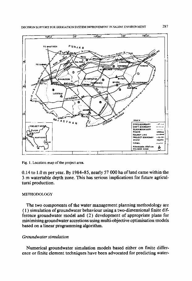
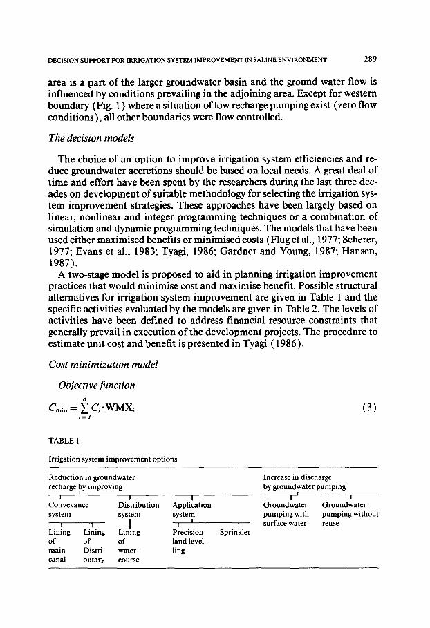
The LGB is located in the northern part of the Indian sub-continent (Fig. 1 ). The River Ghaggar belongs to the Indus River System. The normal annual precipitation varies from 150 to 600 mm, and on the basis of the Thornth- waite classification, the climate of the project area is classified as semi-arid.

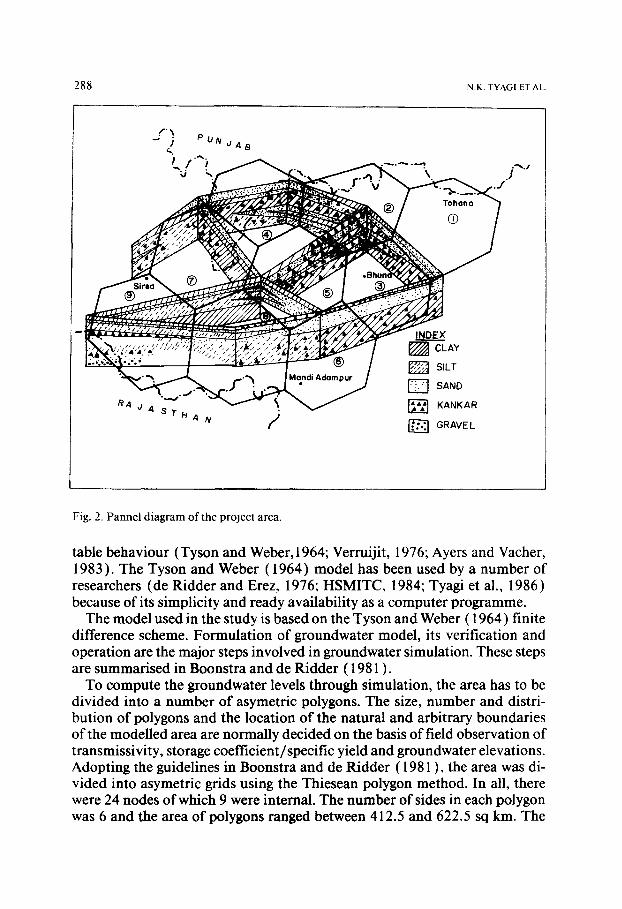
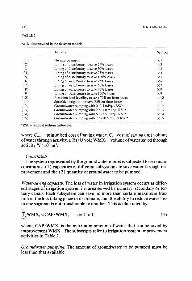
The soils of the basin are of light to medium texture and have been formed under the fluviate agency of the Indo-Gangetic River System. A pannel diagram, prepared on the basis of lithological logs of boreholes to a depth of 275 m (Fig. 2) suggests that the alluvial deposits occur in irregular shape and have different grades of sand varying from medium to very fine along with clay beds on a regional scale.

The quality of groundwater in aquifer zones of the region varies both in vertical and lateral directions. The estimated proportion of fresh (EC < 2dS/ m), marginal (EC 2-6dS/m) and saline ( E C > 6 d S / m ) groundwater is 12, 53 and 35%, respectively. The groundwater also has the sodicity problem.

Introduction of canal irrigation in the area on a large scale occurred around 1954, when Bhakra reservoir was commissioned. Uncontrolled application of water led to increased groundwater accretions and consequently rise in water levels. Land terrain is very fiat with a gradient of only 0.5 per km. The natural drainage of the area is insufficient and the presence of thick clay layers at 100 m depth further compounds the problem. Since the aquifer formation is poor and groundwater is of poor quality, development of groundwater for irrigation has not taken place. As a result the watertable rises at rates varying from

DECISION SUPPORT FOR IRRIGATION SYSTEM IMPROVEMENT IN SALINE ENVIRONMENT 287

• ~*1o' I,~' ,~1~o' 1,8' ,,01o'

TO SHATINOA P U N d A 8

' ; . f- /.,.7

• ........ ,,,,/

- o r , 4 ~ ,,_Z~.. "'.~o ~'~" ° " ~; ...-",. __~;~* ,~Ex I STATE BOUNDARY -'~ "' -- PROJECT AR DISTT BOUNDARY . . . . .

1 ~ BLOCK BOUNDARY ....... ROADS ~ • RAILWAY LINE

_ I I I I I

Fig. 1. Location map of the project area.

0.14 to 1.0 m per year. By 1984-85, nearly 57 000 ha of land came within the 3 m watertable depth zone. This has serious implications for future agricultural production.

METHODOLOGY

The two components of the water management planning methodology are ( 1 ) simulation of groundwater behaviour using a two-dimensional finite difference groundwater model and (2) development of appropriate plans for minimising groundwater accretions using multi-objective optimisation models based on a linear programming algorithm.

Groundwater simulation

Numerical groundwater simulation models based either on finite difference or finite element techniques have been advocated for predicting water-

288 N.K. TYAGI ET AL.

) PUNj4B

/ z "~ :%. , ,

I _ j s,No I " " o 4 s - - - ~ ~" ~ ~ KANKAR

Fig. 2. Pannei diagram of the project area.

table behaviour (Tyson and Weber, 1964; Verruijit, 1976; Ayers and Vacher, 1983). The Tyson and Weber (1964) model has been used by a number of researchers (de Ridder and Erez, 1976; HSMITC, 1984; Tyagi et al., 1986) because of its simplicity and ready availability as a computer programme.

The model used in the study is based on the Tyson and Weber (1964) finite difference scheme. Formulation of groundwater model, its verification and operation are the major steps involved in groundwater simulation. These steps are summarised in Boonstra and de Ridder ( 1981 ).

To compute the groundwater levels through simulation, the area has to be divided into a number of asymetric polygons. The size, number and distribution of polygons and the location of the natural and arbitrary boundaries of the modelled area are normally decided on the basis of field observation of transmissivity, storage coefficient/specific yield and groundwater elevations. Adopting the guidelines in Boonstra and de Ridder ( 1981 ), the area was divided into asymetric grids using the Thiesean polygon method. In all, there were 24 nodes of which 9 were internal. The number of sides in each polygon was 6 and the area of polygons ranged between 412.5 and 622.5 sq km. The


area is a part of the larger groundwater basin and the ground water flow is influenced by conditions prevailing in the adjoining area. Except for western boundary (Fig. 1 ) where a situation of low recharge pumping exist (zero flow conditions), all other boundaries were flow controlled.

The decision models

The choice of an option to improve irrigation system efficiencies and reduce groundwater accretions should be based on local needs. A great deal of time and effort have been spent by the researchers during the last three dec- ades on development of suitable methodology for selecting the irrigation system improvement strategies. These approaches have been largely based on linear, nonlinear and integer programming techniques or a combination of simulation and dynamic programming techniques. The models that have been used either maximised benefits or minimised costs (Flug et al., 1977; Scherer, 1977; Evans et al., 1983; Tyagi, 1986; Gardner and Young, 1987; Hansen, 1987).

A two-stage model is proposed to aid in planning irrigation improvement practices that would minimise cost and maximise benefit. Possible structural alternatives for irrigation system improvement are given in Table 1 and the specific activities evaluated by the models are given in Table 2. The levels of activities have been defined to address financial resource constraints that generally prevail in execution of the development projects. The procedure to estimate unit cost and benefit is presented in Tyagi (1986).

Cost minimization model

Objective function n

Cmin = . E c i - W M X i l = l

(3)

TABLE1

Irrigation system improvement options

Reduction in groundwater recharge by improving

I | I I

Conveyance Distribution Application system system system

i | I I I

Lining Lining Lining Precision of of of land level- main Distri- water- ling canal butary course

I Sprinkler

Increase in discharge by groundwater pumping

I I i

Groundwater Groundwater pumping with pumping without surface water reuse

290

T A B L E 2

Activit ies includedin

N K TYAGIETAL

the decision models

Activity Symbol

( 1 ) No ~mprovement X 1 ( 2 ) Lining of distributary to save 25% losses X 2 (3) Lining of dis t r ibutary to save 50% losses X 3 (4) Lining of distributary to save 75% losses X 4 ( 5 ) Lining of distributary to save 100% losses X 5 (6) Lining of watercourse to save 25% losses X 6 ( 7 ) Lining of watercourse to save 50% losses X 7 (8) Lining of watercourse to save 75% losses X 8 ( 9 ) Lining of watercourse to save 100% losses × 9

( 10 ) Precision land levelling to save 75% on-farm losses x 10 ( 11 ) Sprinkler irr igation to save 25% on-farm losses X 11 ( 12 ) Groundwate r pumping with 0-2.5 m E q / l RSC* X 12 ( 13 ) Groundwate r pumping with 2.5-5.0 m E q / l RSC* X 13 ( 14 ) Groundwate r pumping with 5.0-7.5 mEq/1 RSC* x 14 ( 15 ) Groundwate r pumping with 7.5-10.5 mEq/ I RSC* X 15

*RSC = residual sodium carbonate.

where Cm,n = minimised cost of saving water; C, = cost of saving unit volume of water through activity, i, R s / U vol.; WMXi = volume of water saved through activity "i" 10 3 m 3.

Constraints The system represented by the groundwater model is subjected to two main

constraints: ( l ) capacities of different subsystems to save water through improvement and the (2) quantity of groundwater to be pumped.

Water-saving capacity. The loss of water in irrigation system occurs at different stages of irrigation system, i.e. area served by primary, secondary or ter- tiary canals. Each subsystem can save no more than certain maximum frac- tion of the loss taking place in its domain, and the ability to reduce water loss in one segment is not transferable to another. This is illustrated by:

11

~ WMX, <CAP-WMX, i=1 to 11 (4)

where, CAP.WMX, is the maximum amount of water that can be saved by improvement WMX,. The subscripts refer to irrigation system improvement activities in Table 2.

Groundwater pumping. The amount of groundwater to be pumped must be less than that available:


15 WMXi < GWQk i = 12 to 15 (5)

k = l to4 i = 1 2

where, GWQk is the maximum amount of available groundwater for pumping in quality-category k.

Minimum improvement constraint. The minimum cost solution should be worked out at a given level of saving or pumping of water. The value is based on water balance for the area, the financial resources available and the degree of improvement required:

~WMXi >VMS (6) 1=1

where, VMS is the minimum volume of water that is to be saved.

Non-negativity constraint. For the solution to have meaning, the water saved WMXi must be greater than zero.

~ WMXi>~0 (7) i = l

Benefit maximization model

If there are no financial constraints, the benefits from irrigation system improvement should be maximised. This is done by setting the objective function to maximise the benefits.

Objective function

Bmax --- ~ biWMXi (8) l = l

where, Bmax=maximised value of the objective function (Rs); bi=benefit from a unit of water saved/pumped through activity "i" (Rs/10 3 m3).

System constraint The benefit maximisation model is subjected to the same system con-

straints as the cost minimisation model except that the greater than or equal to constraint of eqn. (6) is changed to an equality ( = ) constraint

n

WMXi = VMS. (9) l = 1

This ensures that the objective function does not become unbounded. These

292 N.K TYAGI ET AL

two models were used to determine the best set of irrigation system improvement activities in each polygon.

MODEL APPLICATION

Groundwater simulation

The groundwater simulation model was calibrated using the available hydrologic data for the LGB area for the period from 1978 to 1983. Necessary adjustments in the model input parameters (the aquifer parameters) were made. Upon getting satisfactory results from calibration, the model was verified for the historical watertable data for the year 1984 (Tyagi et al., 1986 ). The verified model was used to predict monthly watertable values over a period of 16 years from 1984 to 1985 to 1999-2000 for different management conditions.

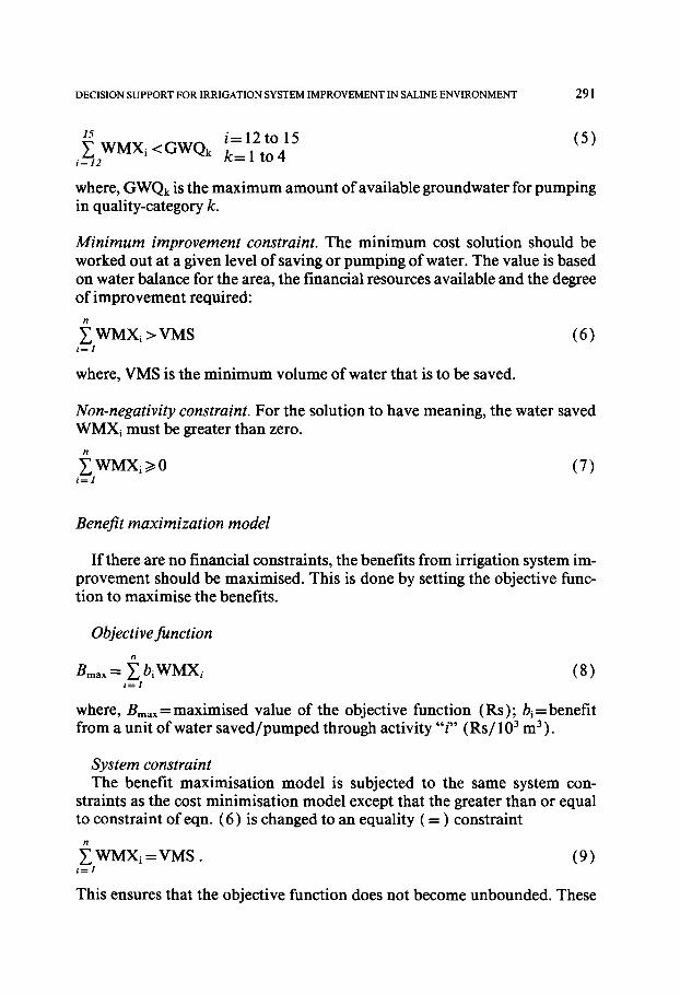
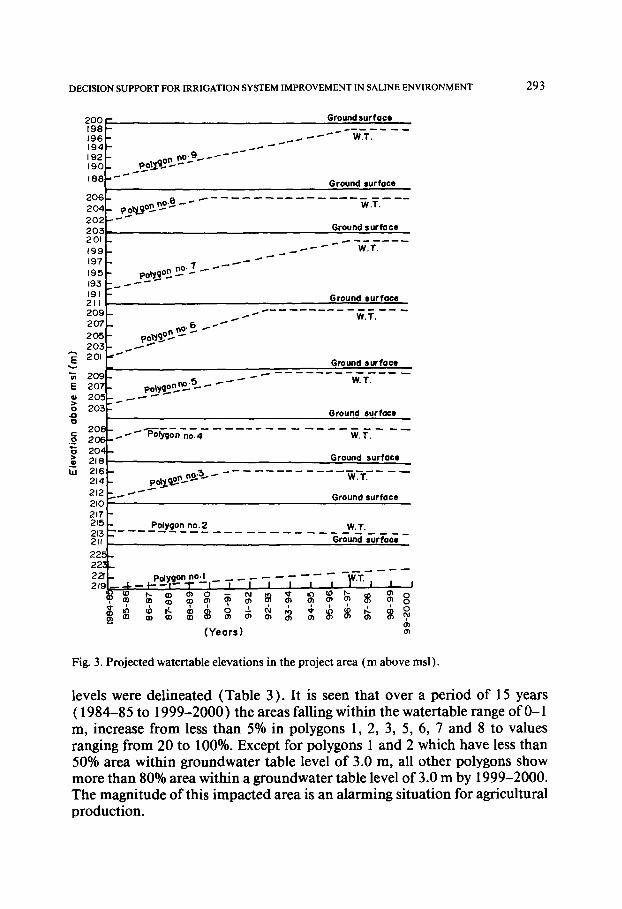
Since the objective of the study was to evaluate the long-term changes in the watertable behaviour, only annual values of the watertable elevations are shown in Fig. 3.

The polygons exhibit varying rates of watertable rise. For example, polygon 2 has a declining trend in watertable at the average rate of 0.04 m/year (Fig. 3 ) whereas polygon 1 has a rise in watertable at the average rate of about 0.2 m/year. Both these polygons lie in an area endowed with aquifer of relatively good water quality with residual sodium carbonate (RSC) level between 4 and 5 mEq/l. As a result, shallow tubewells have been installed by the farmers which extract almost all of the annual recharge in polygon 2 and about 42% in polygon 1.

Polygons 3 and 6 lie in an area, with poor groundwater quality (RSC = 7-8 mEq/1) and relatively poor transmissivity. As a result, less groundwater ( < 30%) is exploited. The recharge from irrigation is comparable to that of polygons 1 and 2. Consequently, the watertable in these polygons shows high rate of annual rise, exceeding 0.7 m/year. The rise of watertable in polygon 4, 5, 8 and 9 is about 0.6 m/year. Predictions indicate that polygon 4 would become static (no further rise in watertable) at a level high enough to cause soil salinisation in 1986-87 followed by polygons 3 and I in 1990-91, polygons 5 and 6 in 1992-93 and polygon 7 in 1996-97 (Fig. 3). The watertable in polygon 1 will continue to rise to the year 2000.

Estimation of waterlogged areas

Based on the model-predicted watertable levels, depth to groundwater contours for the years 1989-90, 1994-95 and 1999-2000 were plotted. Super- imposing these contours on the topographic map of the area, the area of land having watertable between 0 and 1 m and 0 and 3 m, depths to watertable


200 198 196 194 192 190 IBe

20E 204 202 203

Ground surface

201 199 19'7 195 195 191 211 209 207 205 203

E 201

E

IJJ 216 214 212 210

Ground surface

W.T.

Ground surface

Ground surface

Ground surface

2091-r" .... ~ ~ 207 i - poi,jgon no~ 5~ ~ ~ ~ W.T . 205}.- ~ ~ ~ ~

$..*

203 r G roun.d ' su..f faoe

20BI-- .-. ~ ~p'~.-'- . . . . . . . . . . . . . . 2061., ~ olygon no.4 W.T.

/

20 )41-- 21 e L Ground surface

217 215 21,3 211

~ j ~ n 2 * ~ - - - -

. . . . _Po2xg2o_n_*.2 . . . . . . .

W,T.

Ground surface

W.T. Ground surface

22. ~

22,

221 2,~ . - ~ - J ~ - ' , ~ " 4 o ' t , - T ~--i - - I - J - i

~ ~ ® ~o ~ ,~ ~ ~ ~o ~ 6 ' _, ~ ;, ~ , _ o

o~ ( Y e a r s ) e

Fig. 3. Projected watertable elevations in the project area ( m above msl) .

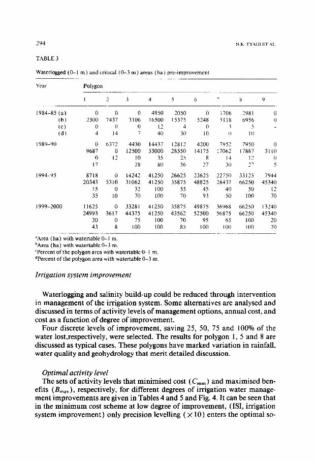
levels were delineated (Table 3). It is seen that over a period of 15 years ( 1984-85 to 1999-2000) the areas falling within the watertable range of 0-1 m, increase from less than 5% in polygons 1, 2, 3, 5, 6, 7 and 8 to values ranging from 20 to 100%. Except for polygons 1 and 2 which have less than 50% area within groundwater table level of 3.0 m, all other polygons show more than 80% area within a groundwater table level of 3.0 m by 1999-2000. The magnitude of this impacted area is an alarming situation for agricultural production.

294

TABLE 3

Waterlogged (0-1 m) and critical (0-3 m) areas (ha) pre-improvement

N.K TYAGI ET AL

Year Polygon

1 2 3 4 5 6 7 8 9

1984-85 (a) 0 0 0 4950 2050 0 1706 2981 0 (b) 2300 7437 3106 16500 15375 5248 5118 6956 0 (c) 0 0 0 12 4 0 ~ 5 - (d) 4 14 7 40 30 I0 I) 10

1989-90 0 6372 4430 14437 12812 4200 7952 7950 0 9687 0 12500 33000 28550 14175 17062 17887 3110

0 12 10 35 25 8 14 12 0 17 28 80 56 27 30 27 5

1994-95 8718 0 14242 41250 26625 23625 22750 33125 7944 20343 5310 31062 41250 35875 48825 28437 66250 45340

15 0 32 100 55 45 41) 50 12 35 10 70 100 70 93 50 100 70

1999-2000 11625 0 33281 41250 35875 49875 36968 66250 13240 24993 3617 44375 41250 43562 52500 56875 66250 45340

20 0 75 100 70 95 65 100 20 43 8 100 100 85 100 100 100 70

"Area (ha) with watertable 0- I m. bArea (ha) with watertable 0-3 m. cPercent of the polygon area with watertable 0-1 m. dPercent of the polygon area with watertable 0-3 m.

Irrigation system improvement

Waterlogging and salinity build-up could be reduced through intervention in management of the irrigation system. Some alternatives are analysed and discussed in terms of activity levels of management options, annual cost, and cost as a function of degree of improvement.

Four discrete levels of improvement, saving 25, 50, 75 and 100% of the water lost,respectively, were selected. The results for polygon 1, 5 and 8 are discussed as typical cases. These polygons have marked variation in rainfall, water quality and geohydrology that merit detailed discussion.

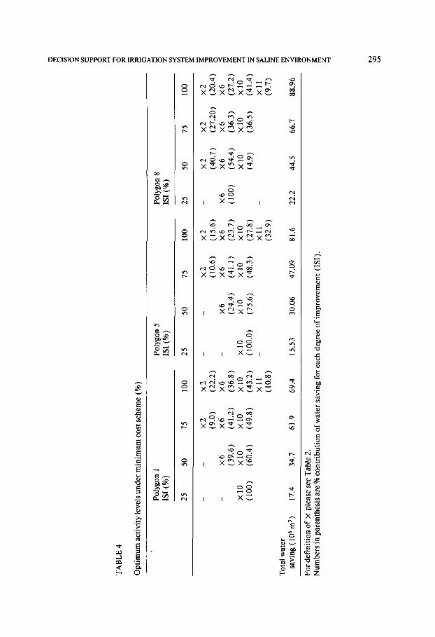
Optimal activity level The sets of activity levels that minimised cost (Cm,n) and maximised ben-

efits (Bin,x), respectively, for different degrees of irrigation water management improvements are given in Tables 4 and 5 and Fig. 4. It can be seen that in the minimum cost scheme at low degree of improvement, (ISI, irrigation system improvement) only precision levelling ( × 10 ) enters the optimal so-

TA

BL

E 4

Opt

imum

act

ivit

y le

vels

und

er m

inim

um c

ost

sche

me

(%)

t~

©

z ©

Pol

ygon

1

Pol

ygon

5

Pol

ygon

8

ISI

(%)

ISI

(%)

ISI

(%)

25

50

75

100

25

50

75

100

25

50

75

100

7~

trt

- -

X2

x2

- -

X2

X2

(9.0

) (2

2.2)

(1

0.6)

(1

5.6)

-

x6

X6

x6

- x6

X

6 x6

(3

9.6)

(4

1.2)

(3

6.8)

(2

4.4)

(4

1.1)

(2

3.7)

x

lO

xlO

x

lO

xlO

x

lO

xlO

x

lO

xlO

(1

00)

(60.

4)

(49.

8)

(43.

2)

(100

.0)

(75.

6)

(48.

3)

(27.

8)

xll

-

xll

(1

0.8)

(3

2.9)

Tot

al w

ater

sa

ving

( 1

06 m

3 )

17.4

34

.7

61.9

69

.4

15.5

3 30

.06

47.0

9 81

.6

X6

(100

)

22.2

x2

(4

0.7)

X

6 (5

4.4)

X

l0

(4.9

)

44.5

X2

(27.

20)

X6

(36.

3)

xlO

(3

6.5)

66.7

x2

(2

0.4)

X

6 (2

7.2)

X

lO

(41.

4)

Xll

(9

.7)

88.9

6

~r

z ,-4

r-

Z t-n

<

For

def

init

ion

of X

ple

ase

see

Tab

le 2

. N

umbe

rs i

n pa

rent

hesi

s ar

e %

con

trib

utio

n of

wat

er s

avin

g fo

r ea

ch d

egre

e of

impr

ovem

ent

(IS

I).

©

I,O

TA

BL

E5

Opt

imum

act

ivit

yle

vel

sun

der

max

imu

m b

enef

itsc

hem

e

Pol

ygon

1

Pol

ygon

5

Pol

ygon

8

ISI

(%)

ISl

(%)

ISl

(%)

25

50

75

100

25

50

75

100

25

50

75

100

- -

X2

X2

- -

x2

×

2

-

(2

9.

5)

(2

2.2)

(2

7.4)

(2

0.5)

-

- X

6

X6

-

- x

6

X6

-

(15.

7)

(36.

7)

(8.3

) (3

1.1)

x

lO

×1

0

XlO

x

lO

xlO

X

lO

xlO

X

lO

×1

0

(56.

4)

(73.

5)

(40.

3)

(30.

2)

(15.

53)

(75.

8)

(48.

8)

(36.

7)

(100

.0)

xll

x

ll

×11

×

11

- ×

11

xll

X

ll

- (4

3.6)

(2

6.5)

(1

4.5)

(1

0.9)

(2

4.2)

(1

5.51

(1

1.7)

Tot

al w

ater

sa

ving

( 1

06 m

s )

17.4

34

.8

For

def

init

ion

of X

ple

ase

see

Tab

le 2

.

52.2

69

.6

30.0

60

.0

90.0

.

..

..

..

..

..

..

..

..

..

..

..

..

..

..

..

..

..

..

Num

bers

in

pare

nthe

sis

are

% c

ontm

but,

on o

f w

ater

sav

ing

for

each

deg

ree

of,

mp

rov

emen

t (I

SI)

.

xlO

(8

2.8)

×1

1 (1

7.2)

×6

(3

0.2)

x

lO

(55.

2)

Xll

(1

4.6)

X2

(20.

4)

X6

(2

7.2)

×

10

(4

1.4)

X

ll

(11.

0)

120.

0 22

.2

44.4

66

.6

88.0

.z X

>-

t'"


POLY- I D °i- ;H c

25% 5 o % ; , 5 % ~ooo, t,

POLY- I

A

Ifh -

2 2 5 % 5 0 % 7 5 %

A D

c

100%

Minimum Cost (CMi n)

POLY-5 A A

2 5 % 50% 7 5 %

A - Applicofion system D - Di~nbuhon system C - Conveyoncs system

POLY-8 A A

~00% 2 5 % 5 0 % Z5% tO0%

TCM = I0 s m s Degree of improvement

Moximum Benefits (BMox)

PO LY - 5 A A

no 2 5 % 5 0

Degree of

D

7 5 % I o o %

improvement

POLY- 8

A A A

2 5 % 5 0 % 7 5 % =00%

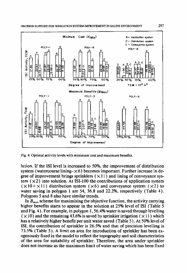
Fig. 4. Optimal activity levels with minimum cost and maximum benefits.

lution. If the ISI level is increased to 50%, the improvement of distribution system (watercourse l in ing -× 6) becomes important. Further increase in degree of improvement brings sprinklers ( X 11 ) and lining of conveyance system ( X 2) into solution. At ISI- 100 the contributions of application system ( X 10 + × 11 ) distribution system ( × 6) and conveyance system ( × 2 ) to water saving in polygon 1 are 54, 36.8 and 22.2%, respectively (Table 4). Polygons 5 and 8 also have similar trends.

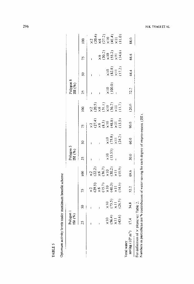
In Bmax scheme for maximising the objective function, the activity carrying higher benefits starts to appear in the solution at 25% level of ISI (Table 5 and Fig. 4). For example, in polygon 1, 56.4% water is saved through levelling ( X 10) and the remaining 43.6% is saved by sprinkler irrigation ( X 11 ) which has a relatively higher benefit per unit water saved (Table 5 ). At 50% level of ISI, the contribution of sprinkler is 26.5% and that of precision levelling is 73.5% (Table 5 ). A limit on area for introduction of sprinkler has been ex- ogenously fixed in the model to reflect the topography and soil characteristics of the area for suitability of sprinkler. Therefore, the area under sprinkler does not increase as the maximum limit of water saving which has been fixed

298 N K. TYAGI ET AL

at 7.56 million cubic meter, is reached at ISI-25% itself. When the ISI is increased to 75%, the lining of conveyance system ( X 2) receives preference in Bmax scheme, unlike the minimum cost solution in which distribution system lining received preference. Lining the conveyance system at ISI-75% contrib- utes to 29.5% of the water saved. At the 100% level of ISI, the contributions of application ( × 10- × 11 ), distribution ( × 6- × 11 ) and conveyance ( × 2- X 5) systems are 41, 22 and 37%, respectively (Table 5) against 34,41 and 25% in the minimum cost model (Table 4 ). The situation in other two polygons is also similar to polygon 1 although the actual values of water saved by different types of improvement varies (Fig. 4 ).

Economic analysis of cost minimisation and benefit maximisation schemes

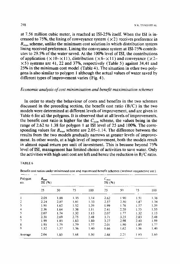
In order to study the behaviour of costs and benefits in the two schemes discussed in the preceding section, the benefit cost ratio (B/C) in the two models were determined at different levels of improvement, and are given in Table 6 for all the polygons. It is observed that at all levels of improvements, the benefit cost ratio is higher for the Cmin scheme, the values being in the range of 2.62 to 1.38 for polygon 1 at ISI level of 25 and 100%. The corresponding values for Bmax scheme are 2.05-1.14. The difference between the results from the two models gradually narrows at greater levels of improvement. In other words, at a high level of improvement, both the models result in almost equal return per unit of investment. This is because beyond 75% level of ISI, management has limited choice of activities to save water. Only the activities with high unit cost are left and hence the reduction in B/C ratio.

TABLE 6

Benefit cost ratios under minimlsed cost and maxlmised benefit schemes (without conjunctive use )

Polygon Bma x Cm, n no. ISI (%) ISI (%)

25 50 75 100 25 50 75 100

1 2.05 1.88 1.35 1.14 2.62 1.90 1.51 1.38 2 2.24 2.07 1.81 1.33 2.57 2.50 1.87 1.34 3 1.91 1.62 1.52 1.39 1.99 1.78 1.57 1.39 4 2.36 1.64 1.38 1.11 2.41 2.20 1.55 1.55 5 2.07 1.74 1.32 1.13 2.07 1.77 1.32 1.13 6 2.31 2.69 2.75 2.48 3.71 3.25 2.83 2.48 7 1.99 1.85 1.83 1.80 3.27 2.98 2.40 1.99 8 1.95 1.79 1.79 1.77 2.01 1.90 1.89 1.77 9 1.52 1.37 1.36 1.40 1.66 1.62 1.56 1.40

Average 2.04 1.85 1.68 1.50 2.48 2.21 1 83 1.60

DECISION SUPPORT FOR IRRIGATION SYSTEM IMPROVEMENT IN SALINE ENVIRONMENT

Effect of lSI on extent of waterlogging

299

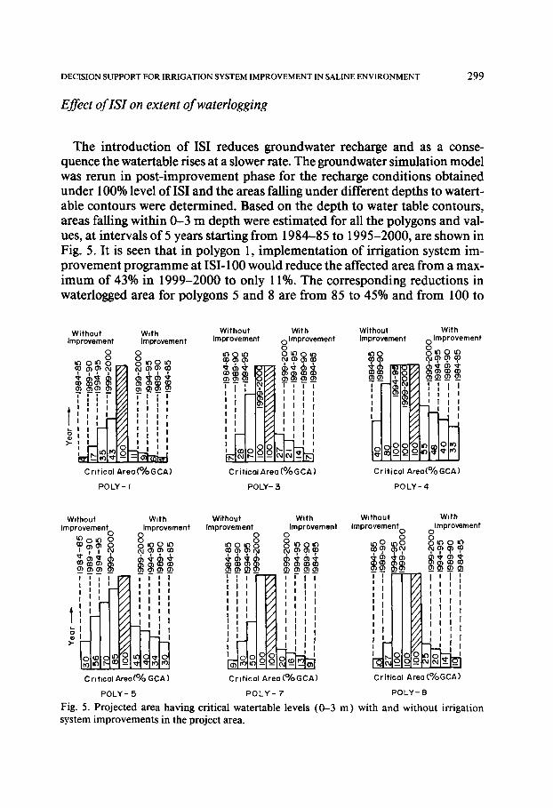
The introduction of ISI reduces groundwater recharge and as a conse- quence the watertable rises at a slower rate. The groundwater simulation model was rerun in post-improvement phase for the recharge conditions obtained under 100% level of ISI and the areas falling under different depths to watertable contours were determined. Based on the depth to water table contours, areas falling within 0-3 m depth were estimated for all the polygons and values, at intervals of 5 years starting from 1984-85 to 1995-2000, are shown in Fig. 5. It is seen that in polygon 1, implementation of irrigation system improvement programme at ISI- 100 would reduce the affected area from a maximum of 43% in 1999-2000 to only 11%. The corresponding reductions in waterlogged area for polygons 5 and 8 are from 85 to 45% and from 100 to

Without Wi th Improvement Improvement

o o o

, ~ 0 3 = o ~ ' ' ' ' ~ 4 6 4 03 0303 0 3 V / 03 T ~ -T "C ~ , . . . . I I I I l i a },~

II

i C I [ I I

Cr i t i ca l Area (°/o G CA)

P O L Y - I

Without With improvement 0 Improvement

0

~ , ~ , o z _ 0 3 ~

- - I I I I 1 I

I

88 '~ Cr i t i ca l Area (°/o G C A )

POLY- -~

Without Improvement

~ 0

03@

i I

C r i t i c a l Areo(°/o GCA)

With 0 Improvement

q J ~ ' . , g g ~ ~,~ 03 ~t , Q ~ 0 3 ~ 0 3

i I , - - 1 I I I

03 I l I I - - ~ I I

P O L Y - 4

Without Improvement

0

4 '4~

II 'H I

With Improvement

~ o=~

I I

i I

C rl tlcal Area (°/o GCA )

Without Wi th Improvement Improvement

0 o

o o o

03=~; ~03 ~ ' 0 3

_ ~ _ _ o~ ~0303

i

C r i t i c a l Area (°/o GCA)

Without Wi th Improvement o olmprovement

0 o

~ ~,~ '

" ; I ' I r t 1 I y , I I "

I I I I I

Cri t ica l Area (° /oGCA)

P O L Y - 5 P O L Y - 7 P O L Y - 8

Fig. 5. Projected area having critical watertable levels (0-3 m) with and without irrigation system improvements in the project area.

3 0 0 N.K. TYAGI ET AL

25%, respectively, over a period of 15 years from 1984-85 through 1999- 2000.

These results quantify the impact of implementation of the system improvement programme. ISI is shown to be quite effective in reducing the extent of affected areas as well as in delaying the occurrence of waterlogging. For example, in pre-improvement phase the affected area in polygon 8 in 1989-90 was 27% compared to only 25% in the year 1999-2000, if improvement were undertaken. Thus, the waterlogging conditions would be post- poned by 10 years. This period is likely to extend further if conjunctive use of saline groundwaters with canal water was practised.

Conclusions

The methodology developed for planning optimal drainable volume reduction to control potential waterlogging is quite general and can be easily ex- trapolated to other areas. Conclusions from this study are as follows:

( 1 ) The groundwater simulation model predicts the watertable level with ad- equate accuracy and can be used for making watertable level projections for 10-15 years in the future.

(2) There is considerable scope for reduction of groundwater accretions by implementing an irrigation system improvement (ISI) programme and thereby minimising production losses. The occurrence of the extent of waterlogging can be delayed by 10-12 years by irrigation system improvements.

( 3 ) The option of reducing groundwater accretions through introduction of ISI has a higher benefit cost ratio up to ISI = 75%. The remaining 25% of the recoverable groundwater recharge should be taken care of by groundwater development and its use with canal water.

(4) Under conditions of financial constraint, improvement of the application subsystem followed by improvement of the distribution and conveyance subsystems are the two most important modifications (in order of priority) for implementing irrigation system rehabilitation programme.

(5) The differential rate of rise in watertable levels in different areas pro- vides a guide for staggering the investment in irrigation system improvements.

REFERENCES

Ayers, J.F. and Vacher, H.L., 1983. A numerical model describing unsteady flow in a fresh water lens. Water Res. Bull., 19: 785-790.

Boonstra, J. and de Ridder, N.A., 1981. Numerical modelling of ground water basra. IILRI, P.O. Box. 6700A Wageningen, The Netherlands, Publication No. 29, p. 226.


de Ridder, N.A. and Erez, E., 1976. Optimum use of water resources, IILRI, The Netherlands, Publication No. 21, p. 250.

Evans, R.G., Walker, W.R. and Skogerboe, G.V., 1983. Strategies for salinity control for the Upper Colorado River Basin. Trans. ASCE, 26: 738-742, 747.

Flug, M., Walker, W.R., Skogerboe, G.V. and Smith, S.W., 1977. The impact of energy development on water resources in the Upper Colorado River Basin, Report to U.S. Department of the Interior, Office of Water Research and Technology, Washington, D.C.

Gardner, R.L. and Young, R.A., 1987. Assessing strategies for control of irrigation induced salinity in the Upper Colorado River Basin. Am. J. Agric. Econ., 69: 37-49.

Hansen, B.R., 1987. A systems approach to drainage reduction, Calif. Agric., 41:19-24. Haryana State Minor Irrigation Tubewell Corporation (HSMITC), 1984. Appraisal document

on studies for use of saline water in canal command areas of irrigation projects, Haryana, Chandigarh, India.

Scherer, C.R., 1977. Water allocation and pricing for control of irrigation related salinity in river basin. Water Res. Res., 13: 225-238.

Tyagi, K.C., Pillai, N.N. and Tyagi, N.K., 1986. Groundwater simulation for planning salinity management. Proceedings of the National Symposium on Hydrology, University of Roor- kee, India, Dec. 16-18, I: V-52-67.

Tyagi, N.K., 1986. Optimal water management strategies for salinity control. J. Irrig. Drain. Eng. ASCE, 112: 81-87.

Tyson, H.N. and Weber, E.M., 1964. Use of electronic computer in the simulation of dynamic behaviour of groundwater basin. Proc. ASCE Water Resources Conference, Milwaukee, Wis- consin, USA.

Verruijit, A., 1972. Solution of transient groundwater flow problems by the finite dement method. Water Res. Res., 8: 725-727.

decision support for irrigation system improvement in saline environment

Documents