Debt Relief or Debt Restructuring? Evidence from an Experiment

with Distressed Credit Card Borrowers∗

Will DobbiePrinceton University and NBER

Jae SongSocial Security Administration

August 2016

Abstract

This paper reports results from a randomized field experiment that offered distressed creditcard borrowers more than $50 million in debt forgiveness and over 27,500 additional monthsto repay their debts. The experimental variation effectively randomized debt write-downs andminimum payments for borrowers at eleven large credit card issuers. Merging information fromthe experiment to administrative tax and bankruptcy records, we find that the debt write-downsincreased debt repayment and decreased bankruptcy filing. The debt write-downs also increasedformal sector employment for the most financially distressed borrowers. In contrast, we find littleimpact of the lower minimum payments on debt repayment, bankruptcy, or employment. Weshow that this null result can be explained by the positive short-run effect of increased liquiditybeing offset by the unintended, negative effect of exposing borrowers to more default risk. Weconclude that debt relief is more effective than debt restructuring for distressed credit cardborrowers, even when these borrowers are liquidity constrained.

∗We are extremely grateful to Ann Woods and Robert Kaplan at Money Management International, David Jones atthe Association of Independent Consumer Credit Counseling Agencies, Ed Falco at Auriemma Consulting Group, andGerald Ray and David Foster at the Social Security Administration for their help and support. We thank Tal Gross,Matthew Notowidigdo, and Jialan Wang for providing the bankruptcy data used in this analysis. We also thank HankFarber, Paul Goldsmith-Pinkham, Tal Gross, Larry Katz, Ben Keys, Patrick Kline, Alex Mas, Jesse Shapiro, AndreiShleifer, Crystal Yang, Jonathan Zinman, Eric Zwick, and numerous seminar participants for helpful comments andsuggestions. Daniel Herbst, Disa Hynsjo, Samsun Knight, Kevin Tang, Daniel Van Deusen, Amy Wickett, and YiningZhu provided excellent research assistance. Financial support from the Washington Center for Equitable Growth isgratefully acknowledged. Correspondence can be addressed to the authors by e-mail: wdobbie@princeton.edu [Dobbie]or jae.song@ssa.gov [Song]. Any opinions expressed herein are those of the authors and not those of the Social SecurityAdministration.

During the 2007-2009 financial crisis, both lenders and policymakers introduced a series of new

debt relief and debt restructuring programs to help distressed borrowers. For example, in the

mortgage market, policymakers implemented reforms such as the Home Affordable Modification

Program (HAMP) that combined elements of both debt relief and debt restructuring in an attempt

to decrease the number of new foreclosures. Over the same time period, a number of large credit

card issuers independently introduced a similar set of debt relief and debt restructuring programs

to decrease the number of new delinquencies, although their efforts were hampered by government

regulations that prevented principal write-downs for most cardholders.1 In both markets, however,

there was little agreement about whether distressed borrowers were most likely to benefit from debt

relief, debt restructuring, or a combination of both.

The relative effectiveness of debt relief and debt structuring depends on the types of constraints

borrowers face at the margin. Debt write-downs benefit borrowers to the extent that long-run

insolvency concerns, and not short-run liquidity constraints, determine borrower behavior at the

margin. Conversely, restructuring debt contracts to reduce or defer payments can address any

short-run liquidity constraints, but at the cost of extending the repayment period and exposing

borrowers to new default risk in the future. To date, there is little empirical evidence on which

type of debt modification is most likely to benefit borrowers in practice.2

This paper provides new evidence on this question using data from a large randomized field

experiment matched to administrative tax and bankruptcy records. The experiment was designed

and implemented by a large non-profit credit counseling organization in the context of a preexist-

ing repayment program, called the Debt Management Plan (DMP). The DMP allows distressed

borrowers to simultaneously repay all of their outstanding credit card debt over a three to five year

period. In exchange for enrolling in the repayment program, credit card issuers will usually lower

the minimum payment amount and provide a partial write-down of any interest payments and

late fees. With more than 600,000 individuals enrolling in these repayment programs each year,

the DMP is one of the most important alternatives to consumer bankruptcy in the United States

(Wilshusen 2011).

In the experiment, control borrowers were offered the status quo repayment program that

had been offered to all borrowers prior to the experiment, while treated borrowers were offered a

modified repayment program that included some combination of two different treatments. The first

1In the United States, banking regulations prevent credit card issuers from simultaneously reducing the originalprincipal and lengthening the repayment period unless a debt is first classified as impaired. During the financial crisis,a group of credit card issuers proposed amending these regulations to allow them to introduce a pilot program thatwould have included both types of debt modifications. Reports indicate that many large card issuers were interestedin participating in the proposed pilot program. For example, see http://www.huffingtonpost.com/2008/10/30/

banks-asking-for-credit-c_n_139478.html2There is both theoretical and empirical work showing that debt relief and debt restructuring can increase

aggregate consumption and employment by decreasing debt overhang, potentially making these policies ex-postefficient during economic downturns (e.g. Hall 2011, Eggertsson and Krugman 2012, Mian, Rao, and Sufi 2013, Mianand Sufi 2014). Debt modifications can also be ex-post efficient in regular economic conditions if debt contracts areincomplete (e.g. Bolton and Scharfstein 1996, Bolton and Rosenthal 2002) or there are negative spillovers of loandefault (e.g. Campbell, Giglio, and Pathak 2011, Mian, Sufi, and Trebbi 2015), although ex-ante responses can offsetthese benefits (e.g. Bolton and Rosenthal 2002, Mayer et al. 2014).

1

treatment increased the typical borrower’s debt write-down amount by an extra $1,712 by dropping

the last four payments of the repayment program and holding the minimum payment constant.

This “debt write-down” treatment is therefore likely to decrease insolvency-based defaults at the

beginning of the repayment program by promising a future debt write-down, and decrease defaults

at the end of the repayment program by deceasing exposure to default risk. Conversely, the second

treatment decreased the typical borrower’s minimum payment amount by an extra $26.68 by adding

an extra four months to the repayment program. This “minimum payment” treatment is therefore

likely to decrease liquidity-based defaults at the beginning of the repayment program by lowering

the minimum payment amount, but increase defaults at the end of the repayment program by

increasing the exposure to default risk. The combination of the two randomized treatments in a

real-world setting makes the experiment an ideal laboratory to measure the effects of debt relief

and debt restructuring.

In total, about 40,000 treated borrowers were offered more than $50 million in new debt write-

downs and more than 27,500 additional months to repay their debts as a part of the experiment.

We measure the effects of the randomized treatments using three administrative datasets matched

for the purposes of this study. Debt repayment is measured using administrative records from the

credit counseling organization that implemented the experiment. Financial distress is measured

using court bankruptcy records. Earnings, employment, and 401k contributions are measured

using tax data from the Social Security Administration (SSA). The matched dataset allows us to

estimate the medium-run effects of the debt write-downs and lower minimum payments across a

range of important outcomes.

We begin our analysis by estimating intent-to-treat effects that measure the impact of being

offered a combination of both treatments. We find that the experiment increased debt repayment

and decreased bankruptcy filing, particularly for borrowers with the highest debt-to-income ratios.

Treatment eligibility increased the probability of finishing a repayment program by 2.97 percentage

points for these high debt-to-income borrowers, a 20.01 percent increase from the control mean.

Bankruptcy filing over the first five years following the experiment also decreased by 1.19 percent-

age points for these borrowers, an 8.40 percent decrease from the control mean. There were no

detectable effects on labor market outcomes or 401k contributions for either high or low debt-to-

income borrowers, although large standard errors mean that we cannot rule out modest treatment

effects in either direction.

While these intent-to-treat estimates show that a more generous repayment program increases

debt repayment and decreases bankruptcy, they do not allow us to identify the separate impact of

debt write-downs and lower minimum payments — the parameters that are most relevant to both

economic theory and policy. Ideally, the experiment would have provided different debt modifi-

cations to different, randomly selected individuals. Some borrowers could have been offered debt

write-downs, but not lower minimum payments. Other borrowers could have been offered lower

minimum payments, but not debt write-downs. In this scenario, we could identify the separate im-

pact of debt write-downs and lower minimum payments by comparing the intent-to-treat estimates

2

across these different treatment groups. However, this experimental design was not feasible for the

non-profit credit counselor implementing the experiment.

We therefore develop an empirical design that identifies the separate impact of each treatment

using the combination of the randomized experiment and the significant across-borrower variation

in potential treatment intensity in our data; that is, the hypothetical write-down and minimum

payment treatments that each borrower in our sample would have received if they had been assigned

to the treatment group. Potential treatment intensity varies across borrowers in our data because

each of the eleven credit card issuers participating in the experiment offered a different combination

of treatments, and because borrowers varied in their propensity to borrower from each of these

credit card issuers. We measure these borrower-specific treatment intensities using detailed data

from the non-profit credit counselor to calculate the difference between each borrower’s hypothetical

treatment and hypothetical control repayment program offers. We then isolate the effects of the

debt write-down and minimum payment treatments by comparing the impact of the randomized

experiment across borrowers that differed in their potential treatment intensity. While our research

design is not a pure experiment (as potential treatment intensity is not randomly assigned to

borrowers), the randomization of treatment eligibility combined with highly accurate measures of

potential treatment intensity allows us to avoid the most likely threats to causal inference.3

Using this empirical design, we find that the debt write-down treatment had an economically

and statistically large effect on most outcomes. For high debt-to-income borrowers, the median

write-down increased the probability of finishing a repayment program by 2.51 percentage points, a

16.91 percent increase from the control mean, and decreased the probability of filing for bankruptcy

in the first five years by 1.37 percentage points, a 9.64 decrease from the control mean. Employ-

ment over the same time period also increased by 1.70 percentage points for high debt-to-income

borrowers, a 2.17 percent increase from the control mean. The estimated effects for earnings and

401k contributions are small and not statistically significant for most borrowers, however.

In sharp contrast, there were no economically or statistically significant effects of the minimum

payment treatment. There was no discernible effect of the minimum payment treatment on debt

repayment, with the 95 percent confidence interval ruling out treatment effects larger than 0.15

percentage points. The median treatment also increased the probability of filing for bankruptcy by

a statistically insignificant 0.70 percentage points, a 6.76 percent increase from the control mean.

There were also no detectable effects of the minimum payment treatment on employment, earnings,

or 401k contributions for any borrowers in our sample.

In the final part of the paper, we use a simple economic model to explore the possible mech-

anisms driving our reduced form results. The model clarifies that the write-down and minimum

3Our empirical strategy is closely related to earlier work using the interaction of state or federal law changes withstate- or individual-level variation in treatment intensity. For example, Card (1992) estimates the impact of minimumwage laws on wages, employment, and education using across-state variation in the fraction of workers earning lessthan a new federal minimum wage. Similarly, Currie and Gruber (1996) estimate the impact of health insuranceeligibility on health care utilization and child health using across-state and across-group variation in the number ofchildren eligible for Medicaid. However, in contrast to these earlier studies, the treatment and control groups in oursetting are determined by random assignment.

3

payment treatments can affect repayment rates through three distinct channels: (1) by decreasing

forward-looking defaults early in the repayment program through the promise of future debt relief,

(2) by decreasing liquidity-based defaults through a lower minimum payment, and (3) by either

decreasing or increasing exposure to default risk at the end of the experiment through either a

shorter or longer repayment program. We then use the model to show that it is possible to test the

relative importance of these competing channels using treatment effects at different points during

the repayment program.

Surprisingly, we find that the effects of the write-down treatment on debt repayment are largely

explained by forward-looking behavior. Taken at face value, our point estimates suggest at least

85.1 percent of the effect of debt write-downs on repayment can be explained by forward-looking

decisions made early in the repayment program. While we are unable to distinguish between the

different types of forward-looking behavior that could be driving our results, these results stand in

stark contrast to the widespread view that distressed credit card borrowers are completely present-

focused.

We also find that the minimum payment treatment modestly decreased liquidity-based defaults

early in the repayment program. However, the positive short-run effect of increased liquidity is

nearly exactly offset by the negative long-run effect of exposing borrowers to more default risk.

The net effect of a lower minimum payment on debt repayment is therefore a statistical zero.

These results help to reconcile our reduced form estimates with a large literature documenting

liquidity constraints in a variety of settings (e.g. Gross and Souleles 2002, Johnson, Parker, and

Souleles 2006, Agarwal, Souleles, and Liu 2007, Parker et al. 2013, Agarwal et al. 2015). We view

our findings as being consistent with this literature, while suggesting that lower minimum payments

are an ineffective way to address liquidity constraints in the credit card market.

Our results are also related to an important literature examining the effect of loan modifica-

tions in the mortgage market. Agarwal et al. (2012) show that mortgage modifications made

through HAMP modestly decreased both mortgage and non-mortgage defaults, although it is un-

clear whether the effects were driven by lower interest rates, principal reductions, or repayment

period extensions.4 Similarly, recent work shows that anticipated mortgage interest rate reductions

during this time period decreased mortgage defaults and increased non-durable consumption (e.g.

Di Maggio, Kermani, and Ramcharan 2014, Keys et al. 2014, Fuster and Willen 2015), although

it is again unclear whether the effects were driven by a lower minimum payment or a lower debt

burden. There are also a number of differences between the secured and unsecured debt markets

that make it difficult to generalize results across these settings. For example, it is possible that liq-

uidity constraints may be relatively more important for mortgage debt, where delinquent borrowers

often have to choose between repayment or foreclosure, while strategic concerns may dominate for

unsecured credit card debt, where borrowers also have the option of filing for bankruptcy (e.g.

4Cross-sectional regressions suggest that principal forgiveness is more effective than other types of mortgagemodifications (Haughwout, Okah, and Tracy 2010), and recent theoretical work suggests that mortgage paymentdeferrals are likely to increase mortgage defaults unless paired with some sort of debt relief (Eberly and Krishnamurthy2014).

4

Mahoney 2015).

Our results are also related to recent work estimating the effects of consumer bankruptcy pro-

tection, which combines elements of both debt relief and debt restructuring for unsecured debts.

Exploiting the random assignment of bankruptcy filings to judges, Dobbie and Song (2015) and

Dobbie, Goldsmith-Pinkham, and Yang (2015) show that bankruptcy protection increases earn-

ings and decreases financial distress, respectively. There is also evidence that the availability of

consumer bankruptcy as an outside option provides implicit health (Gross and Notowidigdo 2011,

Mahoney 2015) and consumption insurance (Dobbie and Goldsmith-Pinkham 2014) to distressed

borrowers, and that filing rates respond to financial incentives (Fay, Hurst, and White 2002). How-

ever, none of these papers are able to identify the mechanisms through which debt relief or debt

restructuring benefits debtors.

There is also a substantial literature on consumer debt more generally. For example, recent

work shows that debt overhang can affect labor supply (Bernstein 2016), entrepreneurial activity

(Adelino, Schoar, and Severino 2013), and home investment (Melzer forthcoming), and that loan

demand is sensitive to interest rates in the credit card (Gross and Souleles 2002), home equity

(Bhutta and Keys 2014), and mortgage markets (DeFusco and Paciorek 2014); to the down payment

amount in the auto loan market (Adams, Einav, and Levin 2009); and to the available loan amount

in the payday loan market (Dobbie and Skiba 2013). There is also work showing that both savings

and borrowing can be affected by the presence of social insurance programs (e.g. Hurst and Ziliak

2006, Hurst and Willen 2007) and by the race of the borrower (e.g. Charles and Hurst 2002,

Charles, Hurst, and Stephens 2008). See Zinman (2015) for a detailed review of the literature.

The remainder of this paper is structured as follows. Section I describes the institutional setting

and experimental design. Section II provides a simple conceptual framework for interpreting the

experimental results. Section III describes our data and empirical design. Section IV presents our

main results of how the randomized experiment affected debt repayment, bankruptcy, labor market

outcomes, and savings. Section V explores the potential mechanisms driving our results. Section

VI concludes.

I. Background and Experimental Design

A. Background

The randomized experiment described in this paper was implemented by Money Management

International (MMI), the largest non-profit credit counseling agency in the United States. In the

early 1950s, credit card issuers helped establish the first non-profit credit counseling organizations

to increase recovery rates and decrease the number of new bankruptcy filings. Today, non-profit

credit counseling organizations such as MMI provide a wide range of services to its clients via phone

and in-person sessions, including general financial advice, credit counseling, bankruptcy counseling,

and housing counseling.

One of the most important products offered by non-profit credit counselors is the debt manage-

5

ment plan (DMP), a structured repayment program that simultaneously repays all of a borrower’s

outstanding credit card debt over three to five years.5 Under the DMP, the credit counseling agency

negotiates directly with each of the borrower’s creditors to lower the minimum payment amount

and partially write-off interest payments and late fees. In most cases, creditors will also agree to

stop recording the debt as delinquent on the borrower’s credit report. The borrower then makes

one monthly payment to the counseling agency that is disbursed to his or her creditors according

to the terms of the restructured agreements. The minimum payment for each credit card account is

typically about two to three percent of the original balance, although borrowers can make additional

payments to reduce the length of the repayment program. In our sample, the average minimum

payment for the control group is 2.38 percent of original balance, or about $437 per month. The

average length of repayment programs for the control group is 52.7 months.

Creditors will usually allow borrowers to resume a repayment program if they miss just one or

two payments. However, if a borrower misses too many payments or withdraws from the program,

the remaining credit card debt is usually sent to collection. At this point, either the original

creditor or a third-party debt collector will use a combination of collection letters, phone calls,

wage garnishment orders, and asset seizure orders to collect the remaining debt. Borrowers can

make these collection efforts more difficult by ignoring collection letters and calls, changing their

telephone number, or moving without leaving a forwarding address. Borrowers can also leave

the formal banking system to hide their assets from seizure, change jobs to force creditors to

reinstate a garnishment order, or work less so that their earnings are not subject to garnishment.

Most borrowers also have the option of discharging the remaining credit card debt through the

consumer bankruptcy system. In all of these scenarios, however, borrowers’ credit scores are likely

to deteriorate significantly, at least in the short run.

The costs of administering the DMP are covered by a combination of a small administrative

fee of about $10 to $50 paid by the borrower, and a “fair share” payment paid by the credit card

issuers. Fair share payments have become somewhat less generous over time, falling from an average

of twelve to fifteen percent of the recovered debt in the 1990s, to about five to ten percent of the

recovered debt today (Wilshusen 2011). To the best of our knowledge, both the fair share payments

and administrative fees remained relatively constant throughout the experiment.

To help ensure that creditors benefit from their participation in the repayment program, the

counseling agency screens potential clients to make sure that (1) the borrower has a sufficient cash

flow to repay his or her debts over the three to five year period of the repayment program, and (2)

that the borrower cannot reasonably repay his or her debts without a repayment program. Histor-

ically, creditors have given credit counseling agencies the incentive to effectively screen potential

clients through a combination of monitoring and the fair share payments discussed above. To

strengthen the counseling agencies’ incentive to effectively screen clients, many creditors also con-

5Under current regulatory guidelines, the term length for a DMP cannot exceed five years. If borrowers cannotfully repay their credit card debts within this five year limit, they cannot participate in a DMP unless the creditor iswilling to write off a portion of the original balance and recognize the loan as impaired. To date, however, creditorshave typically been unwilling to do this (Wilshusen 2011).

6

dition their fair share payments on the borrower’s completion of the repayment program (Wilshusen

2011).

Creditor participation in a DMP is voluntary, and creditors may choose to participate in only

a subset of the DMPs proposed by the credit counseling agencies. In principle, a creditor will only

participate in a repayment program if doing so increases the expected repayment rate, presumably

because the borrower is likely to default or file for bankruptcy (Wilshusen 2011).6 Creditors can

also directly refer borrowers to a credit counseling agency if the risk of default or bankruptcy is

particularly high. In our sample, approximately 15.5 percent of individuals report that they learned

about MMI from a creditor. In comparison, 33.7 percent of individuals in our sample report that

they learned about MMI from an internet search, 19.8 percent from a family member or friend,

and 20.0 percent from a paid advertisement.

Each year, MMI administers over 75,000 DMPs that repay nearly $600 million in unsecured debt.

Nationwide, it is estimated that non-profit credit counselors administer approximately 600,000

DMPs that repay unsecured creditors between $1.5 and $2.5 billion each year (Hunt 2005, Wilshusen

2011).

B. Experimental Design

Overview: In 2003, MMI and eleven large credit card issuers agreed to offer lower minimum pay-

ments and new debt write-downs to a subset of borrowers interested in a structured repayment

program. The purpose of the experiment was to evaluate the effect of more borrower-friendly

terms on repayment rates, particularly for the most financially distressed borrowers.

The resulting randomized experiment was conducted between January 2005 and August 2006.

The experimental population consisted of the approximately 80,000 prospective clients that con-

tacted MMI during this time period. The experiment only included individuals contacting MMI

for the first time during this time period; individuals who had already enrolled in a DMP before

January 2005 were excluded from the randomized trial. Individuals working with counselors with

less than six months of experience were also excluded from the experiment.

Sequence of the Experiment: First, each prospective client was randomly assigned to a credit

counselor conditional on the contact date, the client’s state of residence, and the reference type

(i.e. web vs. phone). For each counselor, the MMI computer system would automatically switch

from the control group concessions to the treatment group concessions every two weeks. This

automated rotation procedure was meant to ensure that experimental procedures were followed by

the counselors, and to ensure that any counselor-specific effects would not bias the experiment.

Counselors were also strictly instructed not to inform prospective clients about the experiment. A

senior credit counselor conducted frequent audits of the counselors to ensure that the experimental

procedures were followed, and that the treatment and control populations remained relatively

6Consistent with this view, individuals enrolled in a DMP are less likely to file for bankruptcy (Staten and Barron2006) and less likely to report financial distress (O’Neill et al. 2006) than observably similar individuals who are notenrolled in a DMP.

7

similar. MMI worked with the participating credit card issuers to design the automated rotation

procedure, but none of the issuers were directly involved with the implementation of the experiment

or the auditing process.

Following the assignment of an individual to a counselor, the assigned counselor collected in-

formation on the prospective client’s unsecured debts, assets, liabilities, monthly income, monthly

expenses, homeownership status, number of dependents, and so on. Identical information was

collected from both the treatment and control groups, and there was no indication of treatment

status communicated to the prospective clients. Using the information collected by the counselor,

the MMI computer system would then calculate the terms of the individual’s repayment program,

including the minimum payment amount, the length of the program, and the total financing costs.

These terms depended on the individual’s specific credit card debts, and whether the individual

was assigned to the treatment or control group.

Next, the credit counselor would explain the individual’s options for repaying his or her debts.

The details of this process closely followed MMI’s usual procedures, and were identical for the

treatment and control groups.7 In most cases, the repayment options were explained in the following

way. First, individuals were told that they could liquidate their assets and repay their debts

immediately, although relatively few individuals in our sample had enough assets to make this a

viable option. Next, individuals were told that they could file for Chapter 7 bankruptcy, which

would allow them to discharge their unsecured debts and avoid debt collection in exchange for any

non-exempt assets and the required court fees. Third, individuals were told what would happen

if they continued paying only the minimum payment on their credit cards. In a representative

call provided to the research team, the MMI counselor explained that “if you continue making the

minimum payment of $350, it will take you 348 months to repay your credit cards, and you will

have to spend about $21,300 in financing charges.” Finally, individuals were told about the benefits

of enrolling in a structured repayment program. In the same representative call, the MMI counselor

explained that if the individual enrolled in a DMP, her payments would “drop to $301, you would

repay all of your credit cards in 56 months, and only have $3,800 in financing charges. That is a

savings of about $17,500.”

Following the counselor’s explanation of the repayment options, the individual would then

indicate whether or not to enroll in the offered repayment program. Individuals could also call

back at a later date to enroll in the repayment program under the same terms.

Treatment Intensity: Compared to control borrowers, treated borrowers were offered repayment

programs with some combination of (1) larger debt write-downs to address any long-run debt

overhang concerns, and (2) lower minimum payments to address any short-run liquidity constraints.

7The internal validity of the experiment is not affected by the details of this procedure, as the framing of therepayment options was identical for treated and control borrowers. Of course, the effects of the two treatments maybe mediated through the specific way the DMP terms were presented to borrowers. For example, it is possible thatindividuals view a debt debt write-down as being more valuable if it is framed as a financing fee reduction. It is alsopossible that individuals view a given treatment as more or less valuable after being told about their outside options.All of our results should be interpreted with these potential framing issues in mind.

8

Table 1 provides an illustrative example of how each treatment could have impacted the typical

borrower’s repayment program. Each row presents DMP terms for a hypothetical borrower with

the mean amount of credit card debt ($18,212), minimum payment requirements (2.38 percent of

initial debt), and interest rate (8.50 percent). We first calculate the DMP terms for the hypo-

thetical borrower under the control conditions. We then recalculate the DMP terms applying the

median write-down treatment (a 3.69 percentage point decrease in the implied interest rate), and

then applying the median minimum payment treatment (a 0.14 percentage point decrease in the

minimum payment percentage).

For this hypothetical borrower, the control repayment program would have required a minimum

payment of $433.45 for 50.05 months, with the financing fees totaling $3,482. The median write-

down treatment would have decreased these financing fees by an additional $1,712, or 49.17 percent,

by dropping the last four payments of the borrower’s repayment program. Importantly, however,

the write-down treatment would not have affected the borrower’s minimum payment amount. As

a result, the treatment should only increase enrollment in the repayment program if borrowers

value debt forgiveness at the end of the repayment program, about three to five years in the

future. The treatment could also increase the probability of completing the repayment program by

mechanically reducing the treatment group’s default rates to zero during the approximately four

month time period when their payments are forgiven.

Conversely, the median minimum payment treatment would have decreased the hypothetical

borrower’s minimum payment by an additional $26.68, or 6.15 percent, by adding an additional

four months to the repayment program. The longer repayment period also would have increased the

financing fees for this borrower by $289, or 8.30 percent. Thus, the minimum payment treatment

should decrease liquidity-based defaults at the beginning of the repayment program by lowering the

minimum payment amount, but increase defaults at the end of the repayment program by increasing

the exposure to default risk. This implies that the net effect of the minimum payment treatment

depends on the relative importance of short-run liquidity constraints and long-run default risk.

The example from Table 1 describes the impact of the median write-down and minimum pay-

ment treatments. In practice, however, there is considerable variation in treatment intensity due to

the different combination of the write-down and minimum payment treatments offered by the eleven

credit card issuers participating in the experiment (see Appendix Table 1). For example, three card

issuers only offered write-down treatment, with all three choosing a different write-down intensity.

While none of the participating issuers offered the minimum payment reduction, one credit card

issuer offered the smallest write-down (i.e. a 4.0 percentage point decrease in the implied interest

rate) and the largest minimum payment reduction (i.e. a 0.5 percentage point decrease in the

minimum payment percentage). In total, seven different combinations of the two treatments were

offered by participating issuers.

Individuals also varied in their propensity to borrow from each of these card issuers, leading

to even more variation in the potential write-down and minimum payment treatments offered to

borrowers. Appendix Figure 1 plots potential treatment intensity for every borrower in our sample.

9

The data reveal significant independent across-borrower variation in the both the write-down and

minimum payment treatments. For example, only 30 percent of borrowers have potential write-

down and minimum payment treatments that are both above the median. Nineteen percent of

borrowers only have an above median potential write-down treatment, and 9.9 percent only have an

above median potential minimum payment treatment. The remainder of the sample have potential

write-down and minimum payment treatments that are both below the median. In total, there

are nearly 50,000 different unique combinations of potential write-down and minimum payment

treatments in our sample.

To illustrate the magnitude of the across-borrower variation in dollar terms, we recalculate the

DMP terms for the hypothetical borrower from Table 1 with various treatment intensities. This

exercise reveals that, for the hypothetical borrower described above, the 75th percentile write-

down treatment is $1,521 larger than the 25th percentile write-down treatment. In other words,

the difference between the 75th and 25th percentile treated borrowers is nearly as large as the

difference between treated and control borrowers at the median. Similarly, the 75th percentile

minimum payment treatment is $33 larger than the 25th percentile minimum payment treatment,

or more than double the difference between treated and control borrowers at the median. In Section

III.C, we explain how we use this variation in treatment intensity to estimate the separate effects

of each treatment.

II. Conceptual Framework

This section develops a simple economic model to better understand the randomized experiment.

The model highlights two broad forms of default risk that may influence borrower behavior: (1)

strategic, forward-looking default risk from debt overhang and (2) non-strategic, liquidity-based

default risk from potentially binding liquidity constraints. We do not attempt to model every

possible mechanism that could affect debt repayment, such as whether the forward-looking default

decisions are due to strategic default or moral hazard in repayment effort. We also do not attempt

to separate these more subtle types of mechanisms empirically. The conclusions we draw in this

section should be interpreted with these modeling choices in mind.8

The model shows how the promise of a future debt write-down increases repayment by (1)

decreasing individuals’ incentive to strategically default at the beginning of the experiment through

increased solvency, and (2) by decreasing individuals’ exposure to default risk at the end of the

experiment through a shorter repayment period. In contrast, a lower minimum payment has an

ambiguous impact on repayment rates due to two competing channels: (1) a decrease in non-

strategic default and an ambiguous change in strategic default at the beginning of the experiment

8A large literature examines the causes and consequences of individual default using quantitative models of thecredit market. For example, see Chatterjee et al. (2007) for a general model of consumer default, and Benjamin andMateos-Planas (2014) for a model that distinguishes between formal and informal consumer default. There is also anemerging literature that estimates the separate impact of different forms of hidden information and hidden action.See Adams et al. (2009) and Karlan and Zinman (2009) for examples of these approaches using observational andexperimental data, respectively.

10

through increased liquidity, and (2) an increase in exposure to default risk at the end of the

experiment through a longer repayment period.

A. Model Setup

We omit individual subscripts from the model parameters to simplify notation. Individuals are risk

neutral and maximize the present discounted value of disposable income at a subjective discount

rate β. In each period t, individuals receive earnings yt = µ + εt, where ε are i.i.d. shocks drawn

from a known mean zero distribution f(ε) and µ is assumed to be both known and positive. Debt

payments begin at t = 0 and are set at a constant level d for the repayment program of length P ,

so that dt = d for t ≤ P and dt = 0 for t > P .

In each time period 0 ≤ t ≤ P , individuals observe their income draw yt and decide whether

to make the required debt payment d or default on the remaining debt payments. If an individual

defaults on the remaining payments in period t for any reason, she loses her current income draw yt

and receives a constant amount x in period t and all future time periods. To capture the idea of a

potentially binding liquidity or credit constraint, we assume that individuals automatically default

if net income yt − dt falls below threshold v , regardless of the value of future cash flows.

Let V q(t, y) denote the continuation value of making repayment decision q in period t given

income draw y. For periods 0 ≤ t < P , the continuation value of default V d(t, y) is equal to the

discounted value of receiving x in both the current period and all future periods:

V d(t, y) =x

1− β(1)

The continuation value of repayment V r(t, y) consists of the contemporaneous value of repayment

y − d and the option value of being able to either repay or default in future periods:

V r (t, y) = y − d+ β

[∫ ∞v+d

max{V r(t+ 1, y

′), V d(t, y)

}dF(y′)

+ F (v + d)V d(t, y)

](2)

The contemporaneous value of repayment y − d is unaffected by the time period t, while the

option value of continuing repayment, and hence the total value of continuing repayment, is weakly

increasing in t for t < P . This is because the option value of repayment increases as individuals

become closer to the “risk-free” time periods after the completion of the repayment program.

Repayment and default behavior is described by a path of cutoff values φt, where an individ-

ual defaults if yt < φt. The default cutoff φt combines the optimal strategic response of liquid

individuals to low income draws and the non-strategic response of illiquid individuals based on v

that may or may not be optimal. Following the above logic, the strategic default cutoff is weakly

decreasing over time, reflecting the decreased incentive to default as individuals’ remaining loan

balances shrink. Appendix A provides additional details on the derivations of the above results.

The reduced form treatment effects documented below likely combine a number of these po-

tential channels. In Section V, we provide a more tentative discussion of which of these broad,

11

competing channels are most important empirically.

B. Model Predictions

Motivated by the experiment, we consider the comparative statics of the write-down and minimum

payment treatments on debt repayment.

Debt Write-Down Prediction: In the model, the write-down treatment increases debt repay-

ment through two complimentary effects: (1) a decrease in treated individuals’ incentive to strate-

gically default while both treatment and control individuals are enrolled in the repayment program,

and (2) a decrease in treated individuals’ exposure to default risk while control individuals are still

enrolled in the repayment program and treatment individuals are not.

Proof – See Appendix A.

Recall that the write-down treatment decreased treated borrowers’ financing charges by short-

ening the repayment period and holding the minimum payment constant. In other words, the

write-down treatment forgave treated borrowers’ monthly payments at the end of the structured

repayment program. As a result, the treatment will increase debt repayment to the extent that

borrowers value debt forgiveness three to five years in the future. Conditional on enrolling in the

program, it is also possible that the write-down treatment will increase the probability of finishing

repayment by decreasing exposure to default risk at the end of the repayment program. This is

because the write-down treatment makes it impossible for treated borrowers to default when their

payments have been forgiven.

Formally, let dWD and PWD denote the monthly debt payment d and repayment period P for

the write-down treatment WD, and dC and PC denote the monthly debt payment and repayment

period for the control group C. In the context of the model, the write-down treatment reduced the

overall cost of the debt by shortening the repayment period for treated individuals relative to control

group individuals, PWD < PC , without changing the monthly debt payments dWD = dC = d. For

0 ≤ t ≤ PWD, shortening the length of the repayment period brings individuals in any given period

PC − PWD periods closer to finishing the repayment program, increasing the expected value of

continuing the repayment program. This increase in the expected value of repayment decreases the

strategic, forward-looking default cutoff for liquid individuals during this time period. However,

disposable income for 0 ≤ t ≤ PWD remains the same, so there is no difference in the probability

that a individual defaults due to the liquidity constraint v during this time period. In other words,

there will only be an increase in repayment for 0 ≤ t ≤ PWD if the forward-looking default cutoff

is the relevant margin for at least some individuals.

For PWD < t ≤ PC , default rates mechanically drop to zero for treated individuals as they have

completed the repayment program. However, control individuals can still default on their debt if

either the liquidity-based or forward-looking cutoffs bind over this time period. The write-down

treatment can therefore increase debt repayment even if individuals never strategically default (i.e.

12

if individuals only default due to a binding liquidity constraint) if there is sufficient default risk at

the end of the repayment program. We refer to this channel as the “exposure effect.”

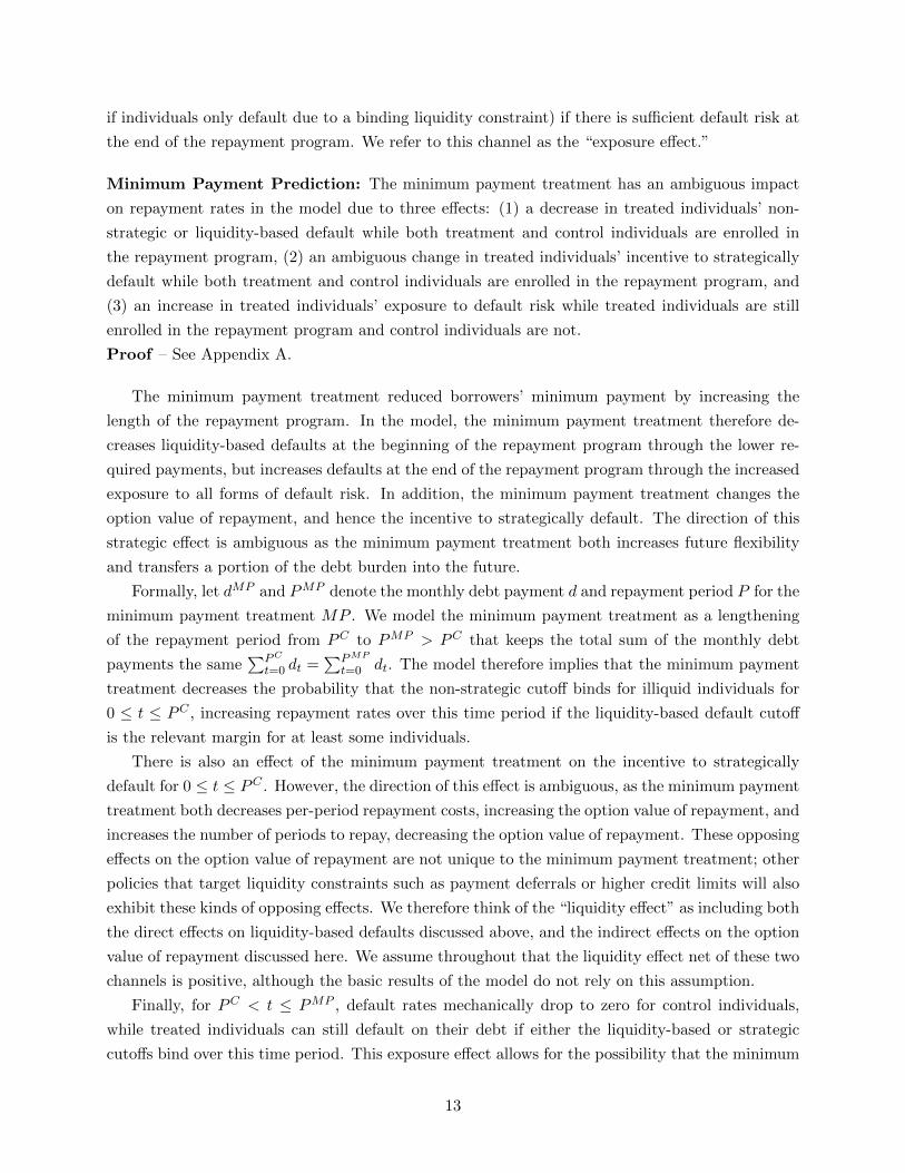
Minimum Payment Prediction: The minimum payment treatment has an ambiguous impact

on repayment rates in the model due to three effects: (1) a decrease in treated individuals’ non-

strategic or liquidity-based default while both treatment and control individuals are enrolled in

the repayment program, (2) an ambiguous change in treated individuals’ incentive to strategically

default while both treatment and control individuals are enrolled in the repayment program, and

(3) an increase in treated individuals’ exposure to default risk while treated individuals are still

enrolled in the repayment program and control individuals are not.

Proof – See Appendix A.

The minimum payment treatment reduced borrowers’ minimum payment by increasing the

length of the repayment program. In the model, the minimum payment treatment therefore de-

creases liquidity-based defaults at the beginning of the repayment program through the lower re-

quired payments, but increases defaults at the end of the repayment program through the increased

exposure to all forms of default risk. In addition, the minimum payment treatment changes the

option value of repayment, and hence the incentive to strategically default. The direction of this

strategic effect is ambiguous as the minimum payment treatment both increases future flexibility

and transfers a portion of the debt burden into the future.

Formally, let dMP and PMP denote the monthly debt payment d and repayment period P for the

minimum payment treatment MP . We model the minimum payment treatment as a lengthening

of the repayment period from PC to PMP > PC that keeps the total sum of the monthly debt

payments the same∑PC

t=0 dt =∑PMP

t=0 dt. The model therefore implies that the minimum payment

treatment decreases the probability that the non-strategic cutoff binds for illiquid individuals for

0 ≤ t ≤ PC , increasing repayment rates over this time period if the liquidity-based default cutoff

is the relevant margin for at least some individuals.

There is also an effect of the minimum payment treatment on the incentive to strategically

default for 0 ≤ t ≤ PC . However, the direction of this effect is ambiguous, as the minimum payment

treatment both decreases per-period repayment costs, increasing the option value of repayment, and

increases the number of periods to repay, decreasing the option value of repayment. These opposing

effects on the option value of repayment are not unique to the minimum payment treatment; other

policies that target liquidity constraints such as payment deferrals or higher credit limits will also

exhibit these kinds of opposing effects. We therefore think of the “liquidity effect” as including both

the direct effects on liquidity-based defaults discussed above, and the indirect effects on the option

value of repayment discussed here. We assume throughout that the liquidity effect net of these two

channels is positive, although the basic results of the model do not rely on this assumption.

Finally, for PC < t ≤ PMP , default rates mechanically drop to zero for control individuals,

while treated individuals can still default on their debt if either the liquidity-based or strategic

cutoffs bind over this time period. This exposure effect allows for the possibility that the minimum

13

payment treatment will have a negative effect on repayment rates.

III. Data and Empirical Design

A. Data Sources and Sample Construction

To estimate the impact of the randomized treatments, we match counseling data from MMI to

administrative tax and bankruptcy records. This section describes the construction and matching

of each dataset.

The counseling data provided by MMI include information on all prospective clients eligible

for the randomized trial. The data include detailed information on each individual’s unsecured

debts, assets, liabilities, monthly income, monthly expenses, homeownership status, number of

dependents, treatment status, enrollment in a repayment program, and completion of a repayment

program. The data also include information on the date of first contact, state of residence, who

referred the individual to MMI, the assigned counselor, and an internal risk score that captures the

probability of finishing a repayment program. We normalize the risk score to have a mean of zero

and standard deviation of one in the control group and top-code all other continuous variables at

the 99th percentile.

We use the data provided by MMI to calculate potential treatment intensity for each individual

in our sample. Recall that there is significant variation in potential debt write-down and minimum

payment treatments as a result of the participating issuers offering different concessions to treated

borrowers. To measure this variation in treatment intensity, we first calculate the write-downs and

minimum payments for all individuals as if they had been assigned to the control group and as

if they had been assigned to the treatment group. In this step, we use the exact calculation that

MMI uses, repeating this calculation under both the control and treatment scenarios. We then

calculate the difference between the control write-downs and the treatment write-downs (in terms

of the implied interest rate) for each individual, and the control minimum payment and treatment

minimum payment (in terms of percent of the original balance) for each individual. These write-

down and minimum payment differences are our individual-level measures of potential treatment

intensity. Importantly, we observe virtually all of the same information that MMI uses to calculate

the terms of the structured repayment program.9

Information on bankruptcy filings comes from individual-level PACER bankruptcy records. The

bankruptcy records are available from 2000 to 2011 for the 81 (out of 94) federal bankruptcy courts

that allow full electronic access to their dockets. These data represent approximately 87 percent of

all bankruptcy filings during our sample period.10 We match the credit counseling data to PACER

data using name and the last four digits of the social security number. We assume that unmatched

9Specifically, we have information on interest rates and minimum payments for the nineteen largest creditors inthe sample, including all eleven of the credit card issuers participating in the experiment. For the 16.7 percent of debtholdings held by smaller creditors not participating in the experiment, we assume an interest rate of 6.7 percent anda minimum payment of 2.25 percent. These assumptions follow MMI’s internal guidelines for calculating expectedDMP payments. Results are also robust to a wide range of alternative assumptions.

10See Gross, Notowidigdo, and Wang (2014) for additional details on the bankruptcy data used in our analysis.

14

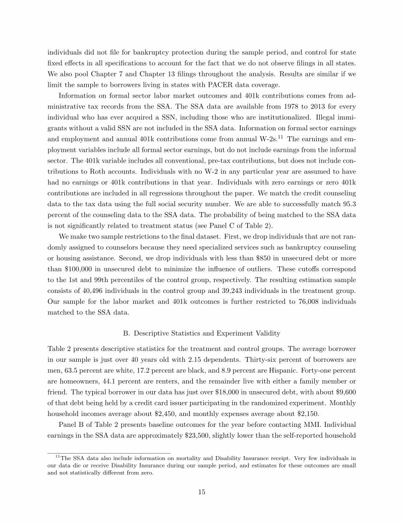
individuals did not file for bankruptcy protection during the sample period, and control for state

fixed effects in all specifications to account for the fact that we do not observe filings in all states.

We also pool Chapter 7 and Chapter 13 filings throughout the analysis. Results are similar if we

limit the sample to borrowers living in states with PACER data coverage.

Information on formal sector labor market outcomes and 401k contributions comes from ad-

ministrative tax records from the SSA. The SSA data are available from 1978 to 2013 for every

individual who has ever acquired a SSN, including those who are institutionalized. Illegal immi-

grants without a valid SSN are not included in the SSA data. Information on formal sector earnings

and employment and annual 401k contributions come from annual W-2s.11 The earnings and em-

ployment variables include all formal sector earnings, but do not include earnings from the informal

sector. The 401k variable includes all conventional, pre-tax contributions, but does not include con-

tributions to Roth accounts. Individuals with no W-2 in any particular year are assumed to have

had no earnings or 401k contributions in that year. Individuals with zero earnings or zero 401k

contributions are included in all regressions throughout the paper. We match the credit counseling

data to the tax data using the full social security number. We are able to successfully match 95.3

percent of the counseling data to the SSA data. The probability of being matched to the SSA data

is not significantly related to treatment status (see Panel C of Table 2).

We make two sample restrictions to the final dataset. First, we drop individuals that are not ran-

domly assigned to counselors because they need specialized services such as bankruptcy counseling

or housing assistance. Second, we drop individuals with less than $850 in unsecured debt or more

than $100,000 in unsecured debt to minimize the influence of outliers. These cutoffs correspond

to the 1st and 99th percentiles of the control group, respectively. The resulting estimation sample

consists of 40,496 individuals in the control group and 39,243 individuals in the treatment group.

Our sample for the labor market and 401k outcomes is further restricted to 76,008 individuals

matched to the SSA data.

B. Descriptive Statistics and Experiment Validity

Table 2 presents descriptive statistics for the treatment and control groups. The average borrower

in our sample is just over 40 years old with 2.15 dependents. Thirty-six percent of borrowers are

men, 63.5 percent are white, 17.2 percent are black, and 8.9 percent are Hispanic. Forty-one percent

are homeowners, 44.1 percent are renters, and the remainder live with either a family member or

friend. The typical borrower in our data has just over $18,000 in unsecured debt, with about $9,600

of that debt being held by a credit card issuer participating in the randomized experiment. Monthly

household incomes average about $2,450, and monthly expenses average about $2,150.

Panel B of Table 2 presents baseline outcomes for the year before contacting MMI. Individual

earnings in the SSA data are approximately $23,500, slightly lower than the self-reported household

11The SSA data also include information on mortality and Disability Insurance receipt. Very few individuals inour data die or receive Disability Insurance during our sample period, and estimates for these outcomes are smalland not statistically different from zero.

15

earnings reported in the MMI data. These results suggest that either some individuals in our sample

are not the sole earner in the household, that some individuals have earnings in the informal sector

not captured by the SSA data, or that there is upward bias in the self-reported earnings. Eighty-

five percent of borrowers in our sample are employed in the formal sector at baseline according to

the SSA data. Baseline bankruptcy rates are very low, 0.3 percent, likely because individuals are

unlikely to contact a credit counselor if they have already received bankruptcy protection. Finally,

baseline 401k contributions are $373 for borrowers in our sample.

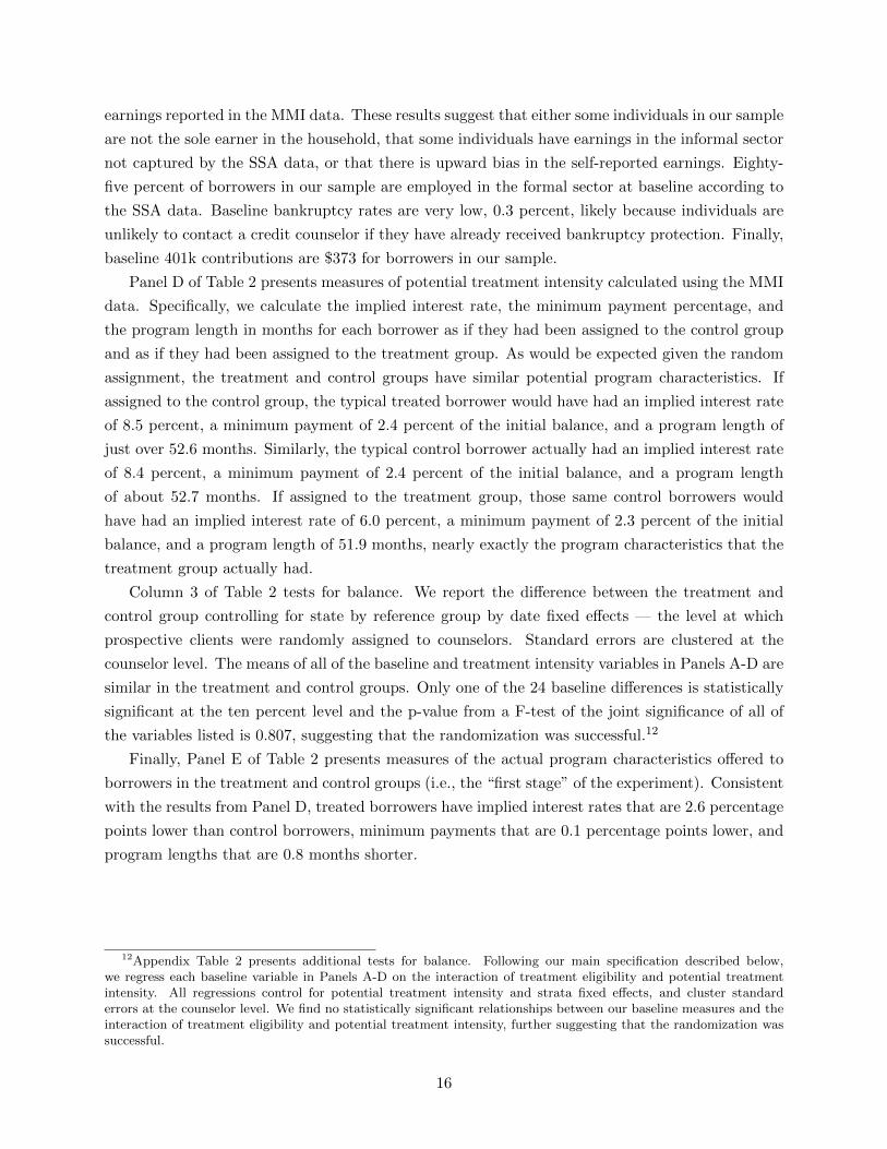
Panel D of Table 2 presents measures of potential treatment intensity calculated using the MMI

data. Specifically, we calculate the implied interest rate, the minimum payment percentage, and

the program length in months for each borrower as if they had been assigned to the control group

and as if they had been assigned to the treatment group. As would be expected given the random

assignment, the treatment and control groups have similar potential program characteristics. If

assigned to the control group, the typical treated borrower would have had an implied interest rate

of 8.5 percent, a minimum payment of 2.4 percent of the initial balance, and a program length of

just over 52.6 months. Similarly, the typical control borrower actually had an implied interest rate

of 8.4 percent, a minimum payment of 2.4 percent of the initial balance, and a program length

of about 52.7 months. If assigned to the treatment group, those same control borrowers would

have had an implied interest rate of 6.0 percent, a minimum payment of 2.3 percent of the initial

balance, and a program length of 51.9 months, nearly exactly the program characteristics that the

treatment group actually had.

Column 3 of Table 2 tests for balance. We report the difference between the treatment and

control group controlling for state by reference group by date fixed effects — the level at which

prospective clients were randomly assigned to counselors. Standard errors are clustered at the

counselor level. The means of all of the baseline and treatment intensity variables in Panels A-D are

similar in the treatment and control groups. Only one of the 24 baseline differences is statistically

significant at the ten percent level and the p-value from a F-test of the joint significance of all of

the variables listed is 0.807, suggesting that the randomization was successful.12

Finally, Panel E of Table 2 presents measures of the actual program characteristics offered to

borrowers in the treatment and control groups (i.e., the “first stage” of the experiment). Consistent

with the results from Panel D, treated borrowers have implied interest rates that are 2.6 percentage

points lower than control borrowers, minimum payments that are 0.1 percentage points lower, and

program lengths that are 0.8 months shorter.

12Appendix Table 2 presents additional tests for balance. Following our main specification described below,we regress each baseline variable in Panels A-D on the interaction of treatment eligibility and potential treatmentintensity. All regressions control for potential treatment intensity and strata fixed effects, and cluster standarderrors at the counselor level. We find no statistically significant relationships between our baseline measures and theinteraction of treatment eligibility and potential treatment intensity, further suggesting that the randomization wassuccessful.

16

C. Empirical Strategy

Intent-to-Treat Estimates: We begin our empirical analysis by estimating the impact of treatment

eligibility using the following reduced form specification:

yit = α0 + α1Treati + α2Xi + ηit (3)

where yit is the outcome of interest for individual i in year t, Treati is an indicator variable equal to

one if individual i was assigned to the treatment group, and Xi is a vector of state by reference group

by date fixed effects that account for the stratification used in the randomization of individuals to

counselors. We also include the individual controls listed in Table 2 and cluster the standard errors

at the counselor level in all specifications. Estimates without individual controls are available in

Appendix Table 3.

Estimates of α1 measure the impact of being offered a more generous repayment program.

However, two important issues complicate the interpretation of these intent-to-treat estimates.

First, treated borrowers were offered a repayment program that included a combination of both the

debt write-down and minimum payment treatments. Thus, the intent-to-treat estimates measure

the combined effect of both treatments, and do not allow us to separately identify the impact of

debt write-downs and lower minimum payments. As a result, it is difficult to extrapolate from the

intent-to-treat estimates to other policies that offer different combinations of debt relief and debt

restructuring.

The second issue is that the intent-to-treat estimates likely understate the true impact of the

debt modifications because of the substantial variation in treatment intensity in our sample. For

example, over 25 percent of borrowers in our sample had zero credit card debt with the eleven credit

card issuers participating in the experiment, and were therefore offered the status quo, or “control”

repayment program even when they were assigned to the treatment group. In total, nearly 90

percent of borrowers received some less intensive treatment than originally intended because they

had at least some credit card debt with a non-participating issuer.

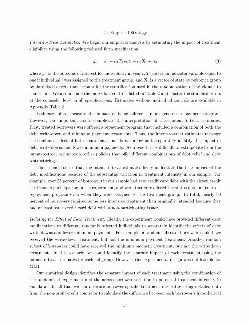
Isolating the Effect of Each Treatment: Ideally, the experiment would have provided different debt

modifications to different, randomly selected individuals to separately identify the effects of debt

write-downs and lower minimum payments. For example, a random subset of borrowers could have

received the write-down treatment, but not the minimum payment treatment. Another random

subset of borrowers could have received the minimum payment treatment, but not the write-down

treatment. In this scenario, we could identify the separate impact of each treatment using the

intent-to-treat estimates for each subgroup. However, this experimental design was not feasible for

MMI.

Our empirical design identifies the separate impact of each treatment using the combination of

the randomized experiment and the across-borrower variation in potential treatment intensity in

our data. Recall that we can measure borrower-specific treatment intensities using detailed data

from the non-profit credit counselor to calculate the difference between each borrower’s hypothetical

17

control and hypothetical treatment repayment program offers. We can then isolate the effects of

write-downs and lower minimum payments using the interaction of the randomized experiment and

these potential treatment intensities. In this specification, we interpret any differences in the effect

of treatment eligibility across borrowers as the independent, causal effect of debt write-downs and

lower minimum payments.

To fix ideas, consider a group of hypothetical borrowers who only borrow from one of two

possible credit card issuers: an issuer that offers treated borrowers only the write-down treatment,

and an issuer that offers treated borrowers both the write-down and minimum payment treatments.

In this simple example, we use the effect of the randomized treatment for borrowers at the first

issuer to identify the impact of the write-down treatment, and the difference between the effects

of the randomized treatment at the second and first issuers to identify the impact of the minimum

payment treatment.

Formally, we define the potential write-down and minimum payment treatment intensities as

the difference between hypothetical treatment and hypothetical control repayment program offers:

∆WriteDowni = WriteDownCi −WriteDownTi

∆Paymenti = PaymentCi − PaymentTi

where ∆WriteDowni is the percentage point difference between the control interest rateWriteDownCiand treatment interest rate WriteDownTi for borrower i, and ∆Paymenti is the percentage point

difference between the control minimum payment percentage PaymentCi and treatment minimum

payment percentage PaymentTi .

We then estimate the effects of the debt write-downs and lower minimum payments using the

following reduced form specification:

yit = β0 + β1Treati ·∆WriteDowni + β2Treati ·∆Paymenti+ β3∆WriteDowni + β4∆Paymenti + β5Xi + εit (4)

We control for any independent effects of ∆WriteDowni and ∆Paymenti because the variation in

these measures may reflect unobserved borrower characteristics that have an independent impact

on future outcomes yit. For example, it is possible that the decision to borrow from card issuers

with particularly high ∆WriteDowni or ∆Paymenti is correlated with risk aversion or financial

sophistication. As will be clear below, our approach does not assume that treatment intensi-

ties are randomly assigned. Rather, we assume that the interaction between treatment eligibility

and potential treatment intensity is conditionally random once we control for ∆WriteDowni and

∆Paymenti. Following the intent-to-treat results, we also include the individual controls listed in

18

Table 2 and cluster the standard errors at the counselor level.13,14

Estimates of β1 and β2 measure the effect of being offered each treatment by comparing the

impact of the randomized experiment across borrowers that differed in their potential treatment

intensities. Our interpretation of the estimates relies on two main assumptions. First, we assume

that treatment eligibility is, in fact, random. As with any non-experimental design, our estimates

will be biased if treatment eligibility is correlated with unobserved determinants of future outcomes

εit. However, this assumption is almost certainly satisfied in our setting, as treatment eligibility is

randomly assigned by the non-profit credit counselor. The balance tests from Table 2 and Appendix

Table 2 are also consistent with random assignment.

Our second identifying assumption is that the interaction of treatment eligibility and (measured)

treatment intensity only impacts borrower outcomes through an increase in (actual) treatment

intensity. Our identifying assumption would be violated if there is measurement error in our

potential treatment intensity variables ∆WriteDowni and ∆Paymenti, and that measurement

error is correlated with unobserved determinants of future outcomes εit. For example, our estimates

would be biased upwards if we systematically overestimate the potential treatment intensity of

borrowers who are most likely to repay their debts even in the absence of the treatment. Fortunately,

we use a nearly identical set of information as the non-profit organization to calculate potential

treatment intensity, making it unlikely that there is the kind of significant measurement error that

would bias our estimates.

Our identifying assumption would also be violated if there is substantial treatment effect het-

erogeneity across borrowers that is correlated with potential treatment intensity. For example,

our estimates would be biased upwards if individuals with a higher LATE from the randomized

treatments were more likely to borrow from the credit card issuers participating in the experiment.

This is because we would attribute the higher estimated effect solely to the higher treatment in-

tensity, not the combination of the higher treatment intensity and the higher LATE. Similarly, our

estimates would be biased downwards if individuals with a lower LATE were more likely to borrow

from the issuers participating in the experiment. These concerns are particularly salient given the

substantial across-borrower dispersion in credit card characteristics documented in prior work (e.g.

Stango and Zinman forthcoming).15

13Equation (4) implicitly assumes that there are no direct effects of treatment eligibility and that the effects of thetwo treatments are linear and additively separable. Consistent with the first assumption, our reduced form results areunchanged when we add an indicator for treatment eligibility. The coefficient on the indicator for treatment eligibilityis also small and not statistically different from zero. To partially test the assumption of linear and additively separabletreatment effects, Appendix Table 4 presents non-parametric estimates using bins of treatment intensity that do notrely on any functional form assumptions. The results are broadly consistent with linear and additively separabletreatment effects, although large standard errors makes a precise test of these assumptions impossible.

14We include all borrowers – including those with no debts with creditors participating in the experiment – whenestimating Equation (4) in order to identify the strata fixed effects. Results are similar if we restrict our sample toindividuals with at least one debt with a participating creditor.

15Appendix Table 5 describes the correlates of potential treatment intensities. Borrowers with larger potentialwrite-down changes are less likely to be black, more likely to be homeowners, and have higher baseline earnings.Borrowers with larger potential minimum payment changes are also less likely to be black, are at lower risk of defaultas measured by MMI’s standardized risk score, and have lower baseline earnings. Not surprisingly, borrowers withmore debt with participating issuers also have larger potential treatment intensities.

19

To partially test the validity of this identifying assumption, Appendix Table 6 examines whether

our potential treatment intensity variables capture all of the relevant variation in the issuer-specific

treatment effects. Our identifying assumption would be violated if there are any significant creditor-

specific treatment effects after we control for the direct effects of treatment intensity. To test this

assumption, we estimate Equation (4) with an additional set of controls for treatment eligibility

interacted with eleven creditor-specific indicator variables equal to one if a borrower has nonzero

debt with the issuer. Consistent with our identifying assumption, the coefficients on the interaction

variables are typically small and not statistically different from zero. In a series of F-tests of the

joint significance of the reported coefficients, the p-values range from 0.369 to 0.986. None of

the results suggest that our identifying assumption is invalid. We will also show below that our

estimates are remarkably similar across gender, race, and homeownership status, suggesting that

our LATEs are relatively similar across observably different borrowers.

Subgroup Analyses: We are also interested in how the effects of the experiment vary across borrower

characteristics such as gender, race, and homeownership. However, we are likely to find a number

of statistically significant estimates purely by chance when performing multiple hypothesis tests.

We were also unable to file a pre-analysis plan, as the experiment was implemented by MMI, and

not the research team. In our main analysis, we therefore restrict ourselves to the single subgroup

analysis suggested by the experimental design: high and low levels of financial distress just prior to

contacting MMI. In the original experimental design, the treatments were only going to be offered

to the most financially distressed borrowers. Following the experiment, many of the credit card

issuers also offered the more borrower-friendly terms only to the most distressed borrowers. To test

how the effects of the experiment differ across this dimension, we estimate effects separately for

borrowers with below and above median debt-to-income. Results are similar if we split borrowers

by debt amount or by the predicted probability of default.16

IV. Results

A. Debt Repayment

Table 3 presents estimates of the impact of being offered larger debt write-downs and lower min-

imum payments on starting and completing a structured repayment program. Panel A reports

intent-to-treat estimates of the impact of treatment eligibility. Panel B reports the coefficient on

treatment eligibility interacted with the potential percentage point change in the implied interest

rate, and treatment eligibility interacted with the potential percentage point change in the required

minimum payment (multiplied by 100). All specifications control for potential treatment intensity,

16Unfortunately we do not have information on the measure of financial distress used by credit card issuersfollowing the experiment. The median unsecured debt-to-annual income ratio in our sample is just over 0.5. AppendixFigure 2 plots repayment rates by debt-to-income ratio. Debt repayment is increasing in debt-to-income ratio untilapproximately 0.75, perhaps because relatively more indebted borrowers have more to gain from the repaymentprogram over this range. Debt repayment then decreases monotonically after a debt-to-income ratio of approximately0.75.

20

the baseline controls listed in Table 2, and strata fixed effects. Standard errors are clustered at the

counselor level throughout.

Intent-to-Treat Results: There is an economically and statistically significant effect of treatment

eligibility on debt repayment. Treatment eligibility increased the probability of starting a repayment

program by 1.86 percentage points, a 5.84 percent increase from the control mean of 31.85 percent.

The probability of finishing a repayment program also increased by 1.33 percentage points, a 9.74

percent increase from the control mean of 13.66 percent.

The effects of treatment eligibility are considerably larger for borrowers with above median

baseline debt-to-income, a proxy for financial distress. Treatment eligibility increased the proba-

bility of starting a repayment program by 1.67 percentage points more for borrowers with above

median debt-to-income compared to borrowers with below median debt-to-income. The probability

of finishing the repayment program also increased by 3.27 percentage points more for borrowers

with above median debt-to-income. These results suggest that, consistent with the priors of MMI

and the credit card issuers, the effects of the two treatments were substantially larger for financially

distressed borrowers.

Appendix Tables 7-9 present additional subsample results by gender, ethnicity, and homeowner-

ship. For each of these three subgroups, there are no clear theoretical predictions as to which group

will benefit most from the experiment. We also do not find any evidence that the intent-to-treat

estimates differ across these subgroups.

Debt Write-Down Results: Consistent with the intent-to-treat estimates discussed above, we find

that the write-down treatment had an economically large impact on repayment rates. The median

write-down treatment (i.e. a 3.69 percentage point implied interest rate reduction) increased the

probability of starting a structured repayment program by 1.85 percentage points, a 5.79 percent

increase from the control mean. The probability of finishing the program also increased by 1.62

percentage points, an 11.89 percent increase from the control mean. In Appendix Figure 3, we

show that the effect of the write-down treatment remains roughly constant throughout the repay-

ment program. Appendix Figure 3 also shows that both treatment and control borrowers exit the

repayment program at high rates, with only 13.66 percent of the control group completely repaying

their debts. In Section V, we will discuss what mechanisms are most consistent with these results.

As with the intent-to-treat estimates, the effects of the write-down treatment are driven by

borrowers with above median debt-to-income. For these high debt-to-income borrowers, the median

write-down treatment increased the probability of starting a repayment program by 2.80 percentage

points, an 8.76 percent change, and increased the probability of finishing a repayment program by

2.51 percentage points, a 16.91 percent change. In comparison, there are no statistically significant

effects of the write-down treatment on borrowers with below median debt-to-income.

To shed light on whether lenders benefit from offering the new debt write-downs, we conduct a

back-of-the-envelope calculation of the expected value of debt with and without the write-downs.

To simplify the calculation, we assume that the lender is risk neutral and does not discount future

21

payments. We also assume that borrowers repay ten percent of any outstanding debt that is not

repaid through the repayment program. Unfortunately, repayment rates outside of the repayment

program are not available in our data. Credit card issuers participating in the experiment suggested

that the average repayment rate for these types of borrowers ranged from 6.5 percent to 14.5 percent

during our sample period.17 Given the wide range of estimates, we also report expected value

calculations assuming repayment rates of zero and twenty percent to explore the robustness of our

results to this assumption.

The average borrower in the control group repays 19.97 percent of his or her debt through the

structured repayment program. Assuming a ten percent repayment rate on the 80.03 percent of debt

that is not repaid through the program, this implies that the average borrower in the control group

repays approximately $5,790 of his or her debt. The median write-down increases the amount repaid

by about 2.0 percent, implying that the average treated borrower repays approximately $5,813 of

his or her debt. Thus, lenders gain approximately $23 for each borrower offered the median write-

down. If the outside repayment rate is zero percent, lenders gain approximately $58 per borrower.

If the outside repayment rate is twenty percent, however, lenders lose approximately $14 for each

borrower offered the median write-down. These calculations suggest that there is likely a modest

ex-post benefit to creditors of offering the new debt write-downs, but that we cannot rule out small

ex-post losses for creditors participating in the experiment. The ex-post benefits to creditors are

also clearly larger if the write-downs were only given to more financially distressed borrowers.

Minimum Payment Results: In sharp contrast to the debt write-down results, we find no effect

of the minimum payment treatment on debt repayment. The point estimates for both starting

and completing a repayment program are small and not statistically different from zero, with the

95 percent confidence intervals ruling out treatment effects larger than 0.24 percentage points for

starting a repayment program and 0.15 percentage points for completing a repayment program.

Appendix Figure 3 shows that these results hold over every percentile of debt repayment. We

also find no effect of lower minimum payments for borrowers with either above or below median

debt-to-income, or among any of the subsample groups we consider in Appendix Tables 7-9.

The null effect of the minimum payment treatment is surprising given a large and influential

literature documenting liquidity constraints in a number of otherwise similar settings (e.g. Gross

and Souleles 2002, Johnson, Parker, and Souleles 2006, Agarwal et al. 2007, Parker et al. 2013).

Our reduced form results suggest that either liquidity constraints are not an important driver of

borrower behavior in our data, or that a lower minimum payment is an ineffective way to alleviate

these liquidity constraints. We return to this issue in Section V.

B. Bankruptcy

Table 4 presents results for bankruptcy filing in the first five years following the experiment, an

important outside option for borrowers in our sample. MMI discusses both the costs and benefits of

17Private communication with MMI and anonymous credit card issuers.

22

bankruptcy with prospective clients, and 10.36 percent of the control group files for bankruptcy in

the first five years following the experiment. Bankruptcy allows most borrowers to discharge their

unsecured debts in exchange for either their non-exempt assets or the partial repayment of debt.

Bankruptcy filings are reported on a borrower’s credit report for seven to ten years, potentially

decreasing access to new credit (Liberman forthcoming) and new employment opportunities (Bos,

Breza, and Liberman 2015). However, conditional on filing, there is evidence that bankruptcy

protection improves recipients’ labor market outcomes, health, and financial well-being (Dobbie and

Song 2015, Dobbie, Goldsmith-Pinkham, and Yang 2015). In our setting, we interpret bankruptcy

as a proxy for general financial distress and the non-repayment of debt.

Intent-to-Treat Results: In the pooled sample, treatment eligibility decreased the probability of

filing for bankruptcy protection by a statistically insignificant 0.31 percentage points over the

first five years following the experiment. Consistent with the repayment results, however, the

effects are larger and more statistically significant for borrowers with above median debt-to-income.

For these high debt-to-income borrowers, treatment eligibility reduced the probability of filing for

bankruptcy by 1.19 percentage points, an 8.40 percent decrease from the control mean. The

effects of treatment eligibility on bankruptcy are larger in the third year following the experiment

(see Appendix Table 10) and prior to the 2005 Bankruptcy Reform BAPCPA that increased the

financial and administrative costs of filing for bankruptcy protection (see Appendix Table 11),

although neither difference is statistically significant due to large standard errors.

Debt Write-Down Results: The effects of treatment eligibility on bankruptcy filing are again driven

by the write-down treatment. Over the first five years following the experiment, the median write-

down decreased the probability of filing for bankruptcy by 0.99 percentage points in the pooled

sample, a 9.61 percent decrease from the control mean of 10.36 percent. The decrease in bankruptcy

filing is again driven by changes in the second and third post-experiment years for the pooled sample,

and the point estimates are again larger prior to the 2005 Bankruptcy Reform. However, neither

difference is statistically significant due to large standard errors.

Consistent with the earlier results, we also find larger effects for borrowers with above median

debt-to-income levels. The median write-down decreased the probability of filing for bankruptcy

by 1.37 percentage points for these high debt-to-income borrowers, a 9.64 percent decrease from

the control mean. The effects for borrowers with below median debt-to-income are much smaller,

although relatively large standard errors means that the difference is not statistically significant

(p-value = 0.152). The bankruptcy effects are also somewhat larger for female and non-white

borrowers, though again neither difference is statistically significant (see Appendix Tables 7-9).

If debt write-downs only impact bankruptcy through increased debt repayment, we could use

treatment eligibility as an instrumental variable for repayment. The resulting two-stage least

squares estimates would measure the local average treatment effect of debt repayment for borrow-

ers induced to repay their debts because of the write-down treatment. These estimates would be

approximately equal to our reduced form bankruptcy estimates divided by the “first stage” repay-

23

ment results presented in Table 3, implying that debt repayment decreases the probability of filing

for bankruptcy by about 46.23 to 61.11 percentage points. Of course, it is likely that debt write-

downs also effect bankruptcy filing through other channels, and that these calculations overstate

the true effects of debt repayment on bankruptcy filing.

Minimum Payment Results: Over the first five years following the experiment, the median minimum

payment reduction increased the probability of filing for bankruptcy by a statistically insignificant

0.70 percentage points, with slightly larger point estimates for borrowers with above median debt-

to-income. In Appendix Table 10, we show that there are statistically significant increases in the

probability of filing in the fifth post-experiment year, suggesting that lower minimum payments

may exacerbate financial distress at the end of the repayment program, perhaps due to a longer

term length.

C. Labor Market Outcomes

Table 5 presents results for average employment and earnings over the first five years following the

experiment. The experiment could affect labor market outcomes through a number of different

channels. For example, debt repayment could increase labor supply by decreasing the frequency of

wage garnishment orders that occur when an employer is compelled by a court order to withhold

a portion of an employee’s earnings to repay delinquent debt. The experiment could also impact

labor market outcomes through its effects on credit scores (e.g. Herkenhoff 2013, Bos et al. 2015,

Herkenhoff and Phillips 2015, Dobbie et al. 2016) or productivity (e.g. Mullainathan and Shafir

2013).

Intent-to-Treat Results: There are no effects of treatment eligibility on employment or earnings for

either the pooled sample or the sample of borrowers with above median debt-to-income. We also

find similar (null) effects by gender, ethnicity, and homeownership.

Debt Write-Down Results: The estimated effect of the write-down treatment on employment and

earnings is also small and imprecisely estimated in the pooled sample. The 95 percent confidence

interval for the employment effect ranges from -0.41 to 1.89 percentage points, while the 95 percent

confidence interval for the earnings effect ranges from -$649 to $347. The effect of the write-down

treatment on employment is larger for borrowers with above median debt-to-income, although

the effect on earnings remains small and imprecisely estimated. For these high debt-to-income

borrowers, the median write-down increased average employment by 1.70 percentage points, a 2.17

percent increase from the control mean.

Consistent with our earlier results, we find similar labor market effects by gender, ethnicity, and

homeownership. However, Appendix Table 12 reveals contrasting labor market effects by baseline

employment status. The write-down treatment decreased annual earnings by $2,077 for borrowers

who were not employed in the year prior to the experiment, while having essentially no effect

on borrowers employed at baseline. The employment effects are also negative for nonemployed

24

borrowers, but the point estimate is not statistically significant. These subsample results suggest

that the kind of debt relief provided by the write-down treatment may decrease labor supply for

borrowers most on the margin of any work.

In contrast to the relatively modest labor market effects documented here, Dobbie and Song

(2015) find that Chapter 13 bankruptcy protection increases annual earnings by $5,562 and annual

employment by 6.8 percentage points. There are at least three potential explanations for these con-

trasting results. First, bankruptcy is a much more intensive treatment, with Chapter 13 discharging

approximately 80 to 85 percent of the typical filer’s unsecured debt (Dobbie, Goldsmith-Pinkham

and Yang 2015). In contrast, the median write-down in our experiment only discharges about 9.63

percent of the typical borrower’s unsecured debt. Second, Chapter 13 bankruptcy also protects

future wages from garnishment and allows filers to retain most assets, both of which may have in-

dependent effects on labor market outcomes. Finally, it is possible that bankruptcy protection has

a larger impact on labor market outcomes due to the different populations served by the non-profit

credit counselor and the consumer bankruptcy system.

Minimum Payment Results: The estimated effect of the minimum payment treatment on labor

market outcomes is small and relatively imprecisely estimated across all borrowers, including those

who were not employed at baseline. In the pooled sample, the 95 percent confidence interval for

the employment effect ranges from -1.38 to 0.26 percentage points, and from -$428 to $570 for the

earnings effect. None of the estimates suggest economically meaningful effects of a lower minimum

payment on labor market outcomes.

D. 401k Contributions

Table 6 presents results for average 401k contributions, a proxy for savings, over the first five years

following the experiment. In theory, the experiment could either crowd out savings by increasing

the returns of debt repayment, or increase savings by decreasing financial distress and increasing

employment and earnings.

Intent-to-Treat Results: There are no effects of treatment eligibility on 401k contributions in either

the pooled sample or the sample of borrowers with above median debt-to-income. We also find

similar (null) effects by gender, ethnicity, and homeownership.

Debt Write-Down Results: Consistent with the intent-to-treat estimates, the estimated effect of

the write-down treatment on 401k contributions is small and imprecisely estimated in the pooled

sample, with the 95 percent confidence interval ranging from -$49.20 to $10.09 for the median

write-down. We find similar (null) effects by baseline financial distress, gender, ethnicity, and

homeownership. Consistent with our labor market results, however, we find that the write-down

treatment decreased 401k contributions by $60.14 for nonemployed borrowers. We also find similar

results for borrowers with zero 401k contributions at baseline (see Appendix Table 13). These

25

results suggest that the debt relief provided by the new debt write-downs may decrease savings for

borrowers most on the margin of work, and hence most on the margin of contributing to a 401k.

Minimum Payment Results: The estimated effect of the minimum payment treatment on 401k

contributions is statistically zero in both the pooled and subsample results, with the 95 percent

confidence interval ranging from -$12.00 to $42.80 for the median minimum payment reduction in

the pooled sample.

E. Robustness Checks

We have run regressions with a number of outcomes and subsamples. The problem of multiplicity

can lead one to incorrectly reject some null hypothesis purely by chance. To test the robustness

of our results, we calculate an alternative set of p-values for our full sample results using a non-

parametric permutation test. Specifically, we create 1,000 “placebo” samples where we randomly

re-assign treatment status to individuals within the randomization strata. We then calculate the

fraction of treatment effects from these 1,000 placebo samples that are larger (in absolute value)

than the treatment effects from the true sample.

Appendix Table 14 presents p-values from this nonparametric permutation test. We find that

our main results are robust to this alternative method of calculating standard errors. If anything,

we obtain smaller p-values from the nonparametric permutation procedure than implied by con-

ventional standard errors. Results are similar for borrowers with above median debt-to-income, our

preferred subsample split.

V. An Empirical Test of the Potential Mechanisms

The preceding analysis has generated two new sets of facts on the effects of debt relief and debt

restructuring on repayment rates and related outcomes. First, debt write-downs increase debt

repayment and decrease bankruptcy filing, with some suggestive evidence of employment and sav-

ings effects for certain subsamples. Second, lower minimum payments have little impact on debt

repayment, bankruptcy, employment, or savings.

In this section, we consider the potential mechanisms that can explain these facts. Recall that,

in theory, the write-down treatment can increase repayment by (1) changing borrowers’ forward-

looking repayment decisions early in the repayment program due to the promise of future debt relief,

and (2) by changing borrowers’ mechanical exposure to default risk late in the repayment program.

Conversely, the minimum payment treatment can either increase or decrease repayment by (1)

changing liquidity early in the repayment program, and (2) by changing borrowers’ mechanical

exposure to default risk late in the repayment program. Below, we show that it is possible to test

the relative importance of these competing channels using estimates from different points during

the repayment program.

26

A. Overview

An important implication from the conceptual framework is that we can use treatment effects at

the beginning and end of the repayment program to test the relative importance of a subset of the

competing theoretical channels. First, consider the write-down treatment. The model implies that

we can test the relative importance of forward-looking behavior using treatment effects early in the

repayment program when both treated and control borrowers are still making payments. This is

because control borrowers and treatment borrowers have identical minimum payments early in the

repayment program. As a result, forward-looking behavior is the only explanation for any observed

differences between the two groups early in the program.

Formally, we test for forward-looking behavior using an estimate of repayment at PWD, or

the end of the repayment program for treated but not control individuals. Again, this is a valid

test of forward-looking behavior because treated and control individuals have identical minimum

payments for t ≤ PWD, and therefore have identical exposure to the non-strategic liquidity risk

over this time period. The estimate at PWD is therefore driven solely by forward-looking strategic

behavior. This repayment estimate at PWD is likely a lower bound of the forward-looking effect,

however, as control individuals can still make forward-looking default decisions for PWD < t ≤ PC .

To test the extent to which the write-down effect can be explained by the mechanical exposure

effect at the end of the repayment program, we can then take the difference between the reduced

form effect evaluated at PWD and the reduced form effect evaluated at PC , i.e. the debt completion

effect reported in our main results below. This is because the reduced form effect at PC is at the

end of the repayment program for both treated and control individuals, and therefore combines any

forward-looking effects and any mechanical exposure effects. If the repayment estimate at PWD is,

in fact, a lower bound, then the exposure effect that we calculate is an upper bound of the true

exposure effect.

Now consider the minimum payment treatment. The model implies that we can test for the

liquidity effect using an estimate of repayment at PC , or the end of the repayment program for

control but not treated individuals. For t ≤ PC , both control and treated individuals are enrolled in

the repayment program, but treated individuals have lower minimum payments and subsequently

increased liquidity on the margin. The estimate at PC is therefore driven solely by the direct and

indirect effects of increased liquidity. The reduced form estimate at PC likely measures an upper

bound of the liquidity effect because treatment individuals can still make forward-looking default

decisions in periods PC < t ≤ PMP . Following the logic from above, we can then calculate the

lower bound of the exposure effect for the minimum payment treatment by taking the difference

between the reduced form effect at PMP and the upper bound of the liquidity effect given by the

reduced form effect at PC . The appendix provides additional discussion of these results.

Our approach is similar to the one used by Schmieder, von Wachter, and Bender (2016) to

estimate the effect of nonemployment durations on wage offers, with one important exception.

Nonemployment durations must be estimated relative to some intermediate time period t > 0,

making it possible for differential selection into the sample to bias their estimates. In contrast,

27

we are primarily interested in the forward-looking and liquidity effects of the experiment, both of

which are measured relative to t = 0. Because we include all individuals, including both those that

never enroll in a repayment program and those who enroll but later drop out, our estimates of these

effects are contaminated by dynamic selection over time.

Dynamic selection can, however, bias our estimates of the exposure effect because we are com-

paring treatment effects at different points in time. For example, it is plausible that the write-down

or minimum payment treatments will induce relatively more distressed borrowers to repay their

debts, leading less distressed borrowers to drop out of the repayment program earlier on. This

type of selection might lead to a different composition of treated and control borrowers later in the

repayment program. In this scenario, our estimate of the exposure effect will be biased downwards.

To shed some light on this issue, Appendix Tables 15-16 compare the characteristics of control

and treatment borrowers completing the repayment program. Only one of the 24 baseline differ-

ences is statistically significant at the ten percent level and the p-value from a F-test of the joint

significance of all of the variables listed is 0.986, suggesting that the treatments did not signifi-

cantly alter the composition of borrowers completing the repayment program. Given these results,

it appears unlikely that our estimates of the exposure effect will be significantly biased by dynamic

selection. Nevertheless, our estimates should be interpreted with this caveat in mind.

B. Empirical Implementation

We implement these empirical tests using a five step process. First, we calculate how long the

repayment plan would have been had the individual been assigned to the treatment group and how

long the repayment plan would have been had the individual been assigned to the control group.

The treatment plans are shorter for individuals with relatively larger debt write-downs and longer

for individuals with relatively larger minimum payment reductions. For example, individuals with

the largest write-downs have treatment plans that are up to 20 percent shorter than their control

plans, while individuals with the smallest write-downs and largest minimum payment reductions

have treatment plans that are up to 100 percent longer than their control plans. Second, we create

an indicator for staying enrolled in the repayment program until the minimum of the treatment

plan length and the control plan length. This indicator variable measures payment at PWD for

individuals with the shorter treatment plans (i.e. relatively larger write-downs) and payment at PC

for individuals with the longer treatment plans (i.e. relatively larger minimum payment reductions).

Third, we estimate Equation (4) using this new indicator variable. These reduced form estimates

measure the effect of write-downs at PWD and the effect of lower minimum payments at PC . Fourth,

we take the difference between the reduced form treatment effects for full repayment estimated in

Table 3 and the new reduced form treatment effects estimated at the shorter of PWD and PC .

Finally, we calculate the standard error of the difference by bootstrapping the entire procedure

described above 500 times. We define the standard error of the treatment effect difference as the

standard deviation of the resulting distribution of estimated differences.

28

C. Estimates

Table 7 presents estimates of forward-looking, liquidity, and exposure effects for both treatments.

Column 1 replicates our estimates from column 4 of Table 3, showing the net effect of all channels

on completing repayment. Columns 2-3 report estimates for starting a repayment program at the

minimum of the treatment program length and control program length. Column 4 reports the

difference between column 1 and columns 2-3.

Debt Write-Down Results: We find that the positive reduced form effect of the debt write-down

treatment is likely due to forward-looking behavior at the beginning of the repayment program,

not decreased exposure to risk at the end of the repayment program. Specifically, the estimates

from Table 7 suggest that at least 85.1 percent of the write-down effect is due to the decrease

in forward-looking defaults. Note that these forward-looking defaults include strategic enrollment

decisions, strategic default decisions, and moral hazard in repayment effort, among other forward-

looking mechanisms. Decreased exposure to risk at the end of repayment can explain a maximum

of 14.9 percent of the write-down effect, with the 95 percent confidence interval including estimates

of up to 38.2 percent of the total reduced form effect.

Unfortunately we are unable to distinguish between the different types of forward-looking behav-

ior that could be driving these results. For example, we can not test whether the forward-looking

default decisions are due to strategic default or moral hazard in repayment effort. We also can

not test whether borrowers are making rational forward-looking decisions based on the increase in

future solvency, or non-rational decisions based on some aspect of the experimental design, such as

the framing of the write-down as a reduction in financing fees.

Minimum Payment Results: We find evidence consistent with both liquidity and exposure effects

being important drivers of the reduced form effect of the minimum payment treatment. Lower

minimum payments have a small positive effect of about 0.03 percentage points on debt repayment

through the liquidity channel, with the 95 percent confidence interval including estimates as large

as 0.16 percentage points. In all specifications, any positive effect from increased liquidity is nearly

exactly offset by the negative effect of increased exposure to default risk.

We view these results as suggesting that the null effect of the minimum payment treatment is

due to the unintended negative effect of exposing individuals to more default risk at the end of the

repayment program. This interpretation of the results is also consistent with the prior literature

suggesting that liquidity constraints are an important determinant of individual behavior. We also

emphasize that our modest point estimates for the liquidity effect may be due to the relatively

small payment reductions offered to treated individuals. It is possible that distressed borrowers

benefit disproportionately more from larger increases in liquidity, such as the mortgage rate resets

examined in the prior literature (e.g. Di Maggio et al. 2014, Keys et al. 2014, Fuster and Willen

2015).

29

VI. Conclusion

This paper uses a randomized experiment to estimate the ex-post impact of larger debt write-downs

and lower minimum payments for distressed credit card borrowers. We find that larger debt write-

downs increase debt repayment and decrease bankruptcy filing. There is also suggestive evidence

of positive labor market effects for the most heavily indebted borrowers, but negative labor market

effects for baseline nonemployed borrowers. In contrast, we find little impact of a lower minimum

payment on debt repayment, bankruptcy, or employment. We show that this null result is due

to the unintended negative effect of exposing borrowers to more default risk when the repayment

period is extended due to the lower minimum payments.

Our estimates suggest that there may be important ex-post benefits of debt relief for borrowers.

These results are of particular importance in light of the ongoing debate over the types of debt

modifications that credit card issuers can offer financially distressed borrowers. In the United

States, banking regulations prevent credit card issuers from simultaneously reducing the original

principal and lengthening the repayment period unless a debt is first classified as impaired. If the

original principal is reduced without the debt being classified as impaired, borrowers are required

to pay off the remaining debt in just a few months. During the financial crisis, a group of credit

card issuers proposed amending these regulations to allow them to conduct a pilot program that

would have forgiven up to 40 percent of a credit card borrower’s original principal, restructured

the remaining principal to be repaid over a number of years, and deferred any income taxes owed

on the forgiven principal. However, government regulators rejected the proposal due to concerns

about when delinquent debts would be recognized on the card issuers’ balance sheets. Our results

suggest that the benefits of accepting the proposal may have been substantial.

An important limitation of our analysis is that we are not able to estimate the impact of debt

relief and debt restructuring on ex-ante borrower behavior or ex-ante borrowing costs. There may

also be important ex-post impacts of debt modifications on outcomes such as post-repayment credit

availability that we are unable to measure with our data. Finally, we are unable to test whether the

forward-looking decisions documented in our analysis are due to rational or non-rational decision

making. These questions remain important areas for future research.

There are also two issues that may affect the applicability of our findings to other contexts.

First, the experiment occurred in the context of a structured repayment program offered by a large

non-profit. It is possible that the estimated effects would be different if the debt modifications had

been offered by a credit card issuer or a third-party debt collector. Second, it is possible that the

effects of the debt modifications may be different for secured debts such as auto or mortgage loans

where creditors have the outside option of seizing the collateral, or for student loan debt where

borrowers do not have the outside option of discharging the debt through the consumer bankruptcy

system. All of our results should be interpreted with these potential external validity issues in mind.

30

References

[1] Adams, William, Liran Einav, and Jonathan Levin. 2009. “Liquidity Constraints and Imperfect

Information in Subprime Lending.” American Economic Review, 99(1): 49-84.

[2] Adelino, Manuel, Antoinette Schoar, and Felipe Severino. 2013. “House Prices, Collateral and

Self-Employment.” NBER Working Paper No. 18868.

[3] Agarwal, Sumit, Gene Amromin, Itzhak Ben-David, Souphala Chomsisengphet, Tomasz Pisko-

rski, and Amit Seru. 2012. “Policy Intervention in Debt Renegotiation: Evidence from the

Home Affordable Modification Program.” NBER Working Paper No. 18311.

[4] Agarwal, Sumit, Nicholas Souleles, and Chunlin Liu. 2007. “The Reaction of Consumer Spend-

ing and Debt to Tax Rebates - Evidence from Consumer Credit Data.” Journal of Political

Economy 115(6): 986-1019.

[5] Agarwal, Sumit, Souphala Chomsisengphet, Neale Mahoney, and Johannes Stroebel. 2015.

“Regulating Consumer Financial Products: Evidence from Credit Cards.” Quarterly Journal

of Economics, 130(1): 111-164.

[6] Benjamin, David, and Xavier Mateos-Planas. 2014. “Formal versus Informal Default in Con-

sumer Credit.” Unpublished Working Paper.

[7] Bernstein, Asaf. 2016. “Household Debt Overhang and Labor Supply.” Unpublished Working

Paper.

[8] Bhutta, Neil, and Benjamin J. Keys. 2014. “Interest Rates and Equity Extraction during the

Housing Boom.” Unpublished Working Paper.

[9] Bos, Marieke, Emily Breza, and Andres Liberman. 2015. “The Labor Market Effects of Credit

Market Information.” Unpublished Working Paper.

[10] Bolton, Patrick, and Howard Rosenthal. 2002. “Political Intervention in Debt Contracts.”

Journal of Political Economy, 110(5): 1103-1134.

[11] Bolton, Patrick, and David Scharfstein. 1996. “Optimal Debt Structure and the Number of

Creditors.” Journal of Political Economy, 104(1): 1-25.

[12] Campbell, John Y., Stefano Giglio, and Parag Pathak. 2011. “Forced Sales and House Prices.”

American Economic Review, 101(5): 2108-2131.

[13] Card, David. 1992. “Using Regional Variation in Wages to Measure the Effects of the Federal

Minimum Wage.” Industrial and Labor Relations Review, 46(1): 22-37.

[14] Charles, Kerwin, and Erik Hurst. 2002. “The Transition to Home Ownership and the Black-

White Wealth Gap.” Review of Economics and Statistics, 84(2): 281-297.

31

[15] Charles, Kerwin, Erik Hurst, and Mel Stephens. 2008. “Rates for Vehicle Loans: Race and

Loan Source.” American Economic Review Papers and Proceedings, 98(2): 315-320.

[16] Chatterjee, Satyajit, Dean Corbae, Makoto Nakajima, and Jose-Vıctor Rıos-Rull. 2007. “A

Quantitative Theory of Unsecured Consumer Credit with Risk of Default.” Econometrica,

75(6): 1525-1589.

[17] Currie, Janet, and Jonathan Gruber. 1996. “Health Insurance Eligibility, Utilization of Medical

Care, and Child Health.” Quarterly Journal of Economics, 111(2): 431-466.

[18] DeFusco, Anthony, and Andrew Paciorek. 2014. “The Interest Rate Elasticity of Mortgage

Demand: Evidence From Bunching at the Conforming Loan Limit.” Federal Reserve Board

Working Paper 2014-11.

[19] Di Maggio, Marco, Amir Kermani, and Rodney Ramcharan. 2014. “Monetary Pass-Through:

Household Consumption and Voluntary Deleveraging.” Unpublished Working Paper.

[20] Dobbie, Will, and Paul Goldsmith-Pinkham. 2014. “Debt Protections and the Great Reces-

sion.” Unpublished Working Paper.

[21] Dobbie, Will, Paul Goldsmith-Pinkham, Neale Mahoney, and Jae Song. 2016. “Bad Credit,

No Problem? Credit and Labor Market Consequences of Bad Credit Reports.” Unpublished

Working Paper.

[22] Dobbie, Will, Paul Goldsmith-Pinkham, and Crystal Yang. 2015. “Consumer Bankruptcy and

Financial Health.” NBER Working Paper No. 21032.

[23] Dobbie, Will, and Paige Marta Skiba. 2013. “Information Asymmetries in Consumer Credit

Markets: Evidence from Payday Lending.” American Economic Journal: Applied Economics,

5(4): 256-282.

[24] Dobbie, Will, and Jae Song. 2015. “Debt Relief and Debtor Outcomes: Measuring the Effects

of Consumer Bankruptcy Protection.” American Economic Review, 105(3): 1272-1311.

[25] Eberly, Janice, and Arvind Krishnamurthy. 2014. “Efficient Credit Policies in a Housing Cri-

sis.” Brookings Papers on Economic Activity, 2(2014).

[26] Eggertsson, Gauti B., and Paul Krugman. 2012. “Debt, Deleveraging, and the Liquidity Trap:

A Fisher-Minsky-Koo Approach.” Quarterly Journal of Economics, 127(3): 1469-1513.

[27] Fay, Scott, Erik Hurst, and Michelle White. 2002. “The Consumer Bankruptcy Decision.”

American Economic Review, 92(3): 706-718.

[28] Fuster, Andreas, and Paul Willen. 2015. “Payment Size, Negative Equity, and Mortgage De-

fault.” FRB of New York Staff Report No. 582.

32

[29] Gross, David, and Nicholas Souleles. 2002. “Do Liquidity Constraints and Interest Rates Mat-

ter for Consumer Behavior? Evidence from Credit Card Data.” Quarterly Journal of Eco-

nomics, 117(1): 149-185.

[30] Gross, Tal and Matthew J. Notowidigdo. 2011. “Health Insurance and the Consumer

Bankruptcy Decision: Evidence from Expansions of Medicaid.” Journal of Public Economics,

95(7-8): 767-778.

[31] Gross, Tal, Matthew J. Notowidigdo, and Jialan Wang. 2014. “Liquidity Constraints and

Consumer Bankruptcy: Evidence from Tax Rebates.” Review of Economics and Statistics,

96(3): 431-443.

[32] Hall, Robert E. 2011. “The Long Slump.” American Economic Review, 101(2): 431-469.

[33] Haughwout, Andrew, Ebiere Okah, and Joseph Tracy. 2010. “Second Chances: Subprime

Mortgage Modification and Re-Default.” Federal Reserve Bank of New York Staff Reports No.

417.

[34] Herkenhoff, Kyle. 2013. “The Impact of Consumer Credit Access on Job Finding Rates.”

Unpublished Working Paper.

[35] Herkenhoff, Kyle, and Gordon Phillips. 2015. “How Credit Constraints Impact Job Finding

Rates, Sorting, and Aggregate Output.” Unpublished Working Paper.

[36] Hunt, Robert M. 2005. “Whither Consumer Credit Counseling?” Federal Reserve Bank of

Philadelphia Business Review, 4Q.

[37] Hurst, Erik and Paul Willen. 2007. “Social Security and Unsecured Debt.” Journal of Public

Economics, 91(7-8): 1273-1297.

[38] Hurst, Erik, and Jim Ziliak. 2006. “Do Welfare Asset Limits Affect Household Saving? Evi-

dence from Welfare Reform.” Journal of Human Resources, 41(1): 46-71.

[39] Karlan, Dean, and Jonathan Zinman. 2009. “Observing Unobservables: Identifying Informa-

tion Asymmetries with a Consumer Credit Field Experiment.” Econometrica, 77(6): 1993-

2008.

[40] Keys, Benjamin J., Tomasz Piskorski, Amit Seru, and Vincent Yao. 2014. “Mortgage Rates,

Household Balance Sheets, and the Real Economy.” Columbia Business School Research Paper

No. 14-53.

[41] Liberman, Andres. “The Value of a Good Credit Reputation: Evidence from Credit Card

Renegotiations.” Forthcoming in Journal of Financial Economics.

[42] Johnson, David, Jonathan Parker, and Nicholas Souleles. 2006. “Household Expenditure and

the Income Tax Rebates of 2001.” American Economic Review 96(5): 1589-1610.

33

[43] Mahoney, Neale. 2015. “Bankruptcy as Implicit Health Insurance.” American Economic Re-

view, 105(2): 710-764.

[44] Mayer, Christopher, Edward Morrison, Tomasz Piskorski, and Arpit Gupta. 2014. “Mortgage

Modification and Strategic Behavior: Evidence from a Legal Settlement with Countrywide.”

American Economic Review, 104(9): 2830-2857.

[45] Melzer, Brian. “Mortgage Debt Overhang: Reduced Investment by Homeowners with Negative

Equity.” Forthcoming in Journal of Finance.

[46] Mian, Atif, Amir Sufi, and Francesco Trebbi. 2015. “Foreclosures, House Prices, and the Real

Economy.” Journal of Finance, 70(6): 2587-2634.

[47] Mian, Atif, Kamalesh Rao, and Amir Sufi. 2013. “Household Balance Sheets, Consumption,

and the Economic Slump.” Quarterly Journal of Economics, 128(4): 1687-1726.

[48] Mian, Atif, and Amir Sufi. 2014. “What Explains the 2007-2009 Drop in Employment?” Econo-

metrica, 82(6): 2197-2223.

[49] Mullainathan, Senhil, and Eldar Shafir. 2013. Scarcity: Why Having Too Little Means So

Much. Macmillan.

[50] O’Neill, Barbara, Aimee D. Prawitz, Benoit Sorhaindo, Jinhee Kim, and E. Thomas Garman.

2006. “Changes in Health, Negative Financial Events, and Financial Distress/Financial Well-

Being for Debt Management Program Clients.” Financial Counseling and Planning, 17(2):

46-63.

[51] Parker, Jonathan, Nicholas Souleles, David Johnson, and Robert McClelland. 2013. “Consumer

Spending and the Economic Stimulus Payments of 2008.” American Economic Review, 103(6):

2530-2553.

[52] Schmieder, Johannes F., Till von Wacther, and Stefan Bender. 2016. “The Effect of Unem-

ployment Benefits and Nonemployment Durations on Wages.” American Economic Review,

106(3): 739-777.

[53] Stango, Victor, and Jonathan Zinman. “Borrowing High vs. Borrowing Higher: Price Dis-

persion and Shopping Behavior in the U.S. Credit Card Market.” Forthcoming in Review of

Financial Studies.

[54] Staten, Michael E., and John M. Barron. 2006.“Evaluating the Effectiveness of Credit Coun-

seling.” Unpublished Working Paper.

[55] Wilshusen, Stephanie. 2011. “Meeting the Demand for Debt Relief.” Federal Reserve Bank of

Philadelphia Payment Cards Center Discussion Paper, 11-04.

34

[56] Zinman, Jonathan. 2015. “Household Debt: Facts, Puzzles, Theories, and Policies.” Annual

Review of Economics, 7: 251-276.

35

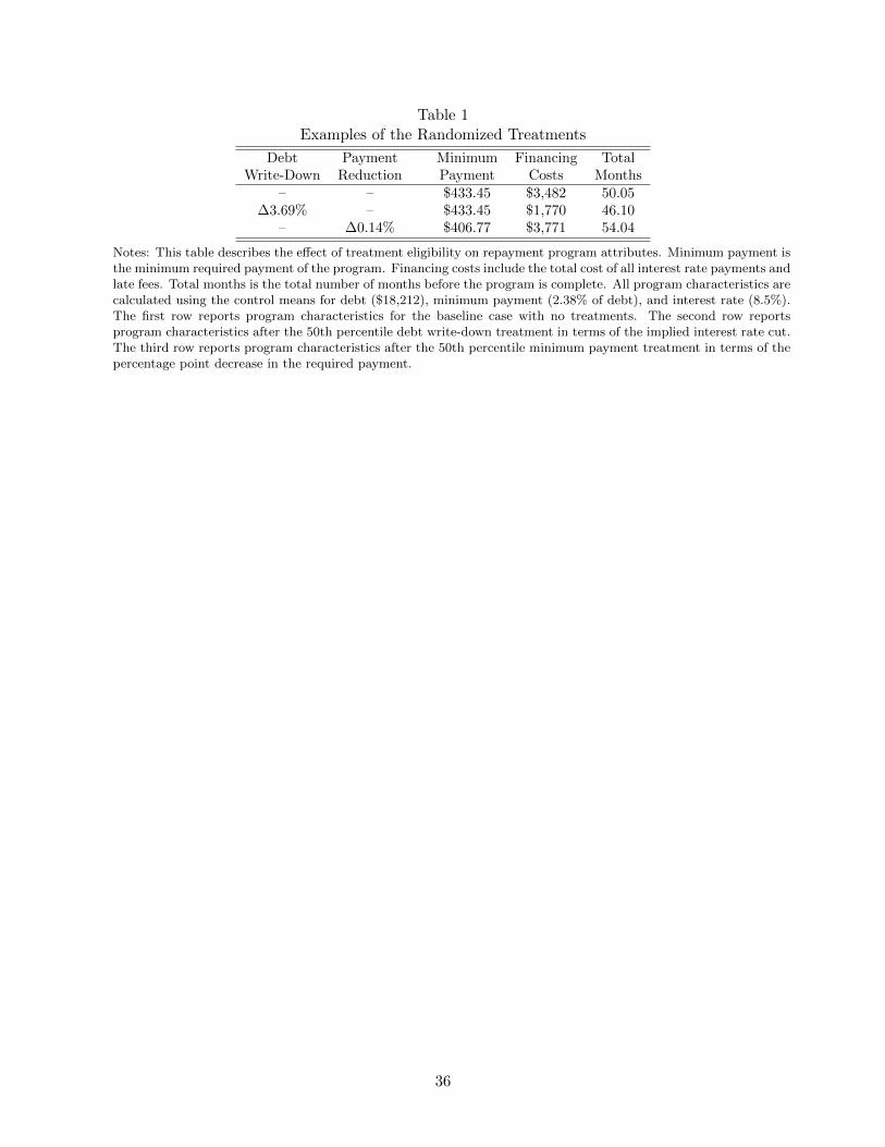
Table 1Examples of the Randomized Treatments

Debt Payment Minimum Financing TotalWrite-Down Reduction Payment Costs Months

– – $433.45 $3,482 50.05∆3.69% – $433.45 $1,770 46.10

– ∆0.14% $406.77 $3,771 54.04

Notes: This table describes the effect of treatment eligibility on repayment program attributes. Minimum payment isthe minimum required payment of the program. Financing costs include the total cost of all interest rate payments andlate fees. Total months is the total number of months before the program is complete. All program characteristics arecalculated using the control means for debt ($18,212), minimum payment (2.38% of debt), and interest rate (8.5%).The first row reports program characteristics for the baseline case with no treatments. The second row reportsprogram characteristics after the 50th percentile debt write-down treatment in terms of the implied interest rate cut.The third row reports program characteristics after the 50th percentile minimum payment treatment in terms of thepercentage point decrease in the required payment.

36

Table 2Descriptive Statistics and Balance Tests

Treatment Control DifferencePanel A: Characteristics (1) (2) (3)

Age 40.626 40.516 −0.271Male 0.363 0.361 0.008White 0.636 0.635 0.010Black 0.171 0.174 −0.008∗

Hispanic 0.090 0.088 −0.001Homeowner 0.412 0.410 −0.003Renter 0.440 0.442 0.003Dependents 2.159 2.156 −0.006Monthly Income 2.453 2.448 0.010Monthly Expenses 2.168 2.158 0.003Total Unsecured Debt 18.212 18.368 0.299Debt with Part. Creditors 9.568 9.615 0.163Internal Risk Score -0.000 -0.003 −0.003

Panel B: Baseline OutcomesBankruptcy 0.004 0.003 −0.001Employment 0.848 0.850 0.004Earnings 23.447 23.518 −0.108Nonzero 401k Cont. 0.227 0.224 −0.006401k Contributions 0.372 0.373 −0.008

Panel C: Data QualityMatched to SSA data 0.953 0.954 0.003

Panel D: Potential Treatment IntensityInterest Rate if Control 0.085 0.084 0.001Interest Rate if Treatment 0.059 0.060 −0.001Min. Payment Percent if Control 0.024 0.024 −0.001Min. Payment Percent if Treatment 0.023 0.023 −0.000Program Length in Months if Control 52.671 52.678 0.058Program Length in Months if Treatment 51.963 51.914 0.036

Panel E: Characteristics of Repayment ProgramInterest Rate 0.085 0.059 −0.026∗∗∗

Min. Payment Percent 0.024 0.023 −0.001∗∗∗

Program Length in Months 52.671 51.914 −0.806∗∗∗

p-value from joint F-test of Panels A-D – – 0.807p-value from joint F-test of Panel E – – 0.000Observations 40,496 39,243 79,739

Notes: This table reports descriptive statistics and balance tests for the estimation sample. Information on age,gender, race, earnings, employment, and 401k contributions is only available for individuals matched to the SSAdata. Risk score is standardized to have a mean of zero and standard deviation of one in the control group. Eachbaseline outcome is for the year before the experiment. Earnings, employment, and 401k contributions come from1978 - 2013 W-2s, where employment is an indicator for non-zero wage earnings. Potential minimum payment andinterest rates are calculated using the amount of debt held by each creditor and the rules listed in Appendix Table 1.All dollar amounts are divided by 1,000. Column 3 reports the difference between the treatment and control groups,controlling for strata fixed effects and clustering standard errors at the counselor level. *** = significant at 1 percentlevel, ** = significant at 5 percent level, * = significant at 10 percent level. The p-value is from an F-test of the jointsignificance of the variables listed.

37

Tab

le3

Deb

tM

od

ifica

tion

san

dR

epay

men

t

Sta

rtP

aym

ent

Com

ple

teP

aym

ent

Fu

llL

owH

igh

Fu

llL

owH

igh

Sam

ple

Deb

t/In

c.D

ebt/

Inc.

Sam

ple

Deb

t/In

c.D

ebt/

Inc.

Pan

elA

:IT

TE

stim

ate

s(1

)(2

)(3

)(4

)(5

)(6

)T

reat

men

tE

ligi

bil

ity

0.0186∗

∗∗0.

0103

0.0270∗

∗∗0.0

133∗

∗∗−

0.00

30

0.0297∗∗

∗

(0.0

057)

(0.0

074)

(0.0

074)

(0.0

044)

(0.0

058)

(0.0

056)

Pan

elB

:D

ebt

Wri

te-D

ow

nan

dM

inim

um

Paym

ent

Est

imate

sD

ebt

Wri

te-D

own

0.0050∗

∗0.

0021

0.0076∗

∗∗0.0

044∗

∗0.

0020

0.0068∗∗

∗

(0.0

023)

(0.0

030)

(0.0

028)

(0.0

017)

(0.0

023)

(0.0

023)

Min

.P

aym

ent

Red

uct

ion

0.0

005

0.0009

0.0001

0.0001

0.0007

−0.

0006

(0.0

006)

(0.0

007)

(0.0

007)

(0.0

005)

(0.0

006)

(0.0

006)

Ob

serv

atio

ns

79,7

39

39,8

69

39,8

70

79,7

39

39,8

69

39,8

70

Mea

nin

Con

trol

Gro

up

0.3

185

0.3

170

0.3

201

0.1

366

0.1

247

0.1

484

Note

s:T

his

table

rep

ort

sre

duce

dfo

rmes

tim

ate

sof

the

impact

of

deb

tm

odifi

cati

ons

on

repay

men

t.In

form

ati

on

on

repay

men

tco

mes

from

adm

inis

trati

ve

reco

rds

at

the

cred

itco

unse

ling

org

aniz

ati

on.

Colu

mns

1and

4re

port

resu

lts

for

the

full

sam

ple

of

borr

ower

s.C

olu

mns

2-3

and

5-6

rep

ort

resu

lts

for

borr

ower

sw

ith

ab

ove

and

bel

owm

edia

ndeb

t-to

-inco

me.

Panel

Are

port

sth

eco

effici

ent

on

trea

tmen

tel

igib

ilit

y.P

anel

Bre

port

sco

effici

ents

on

the

inte

ract

ion

of

trea

tmen

tel

igib

ilit

yand

pote

nti

al

deb

tw

rite

-dow

n(i

nte

rms

of

the

inte

rest

rate

inp

erce

nta

ge

poin

ts),

and

the

inte

ract

ion

of

trea

tmen

tel

igib

ilit

yand

pote

nti

al

min

imum

pay

men

tre

duct

ion

(in

per

centa

ge

poin

tsx

100).

All

spec

ifica

tions

contr

ol

for

pote

nti

al

deb

tw

rite

-dow

n,

pote

nti

al

min

imum

pay

men

tre

duct

ion,

the

base

line

contr

ols

inT

able

2,

and

stra

tafixed

effec

ts,

and

clust

erst

andard

erro

rsat

the

counse

lor

level

.***

=si

gnifi

cant

at

1p

erce

nt

level

,**

=si

gnifi

cant

at

5p

erce

nt

level

,*

=si

gnifi

cant

at

10

per

cent

level

.See

Table

2note

sfo

rdet

ails

on

the

base

line

contr

ols

and

sam

ple

.

38

Table 4Debt Modifications and Bankruptcy Filing

Bankruptcy in Years 1-5Full Low High

Sample Debt/Inc. Debt/Inc.Panel A: ITT Estimates (1) (2) (3)

Treatment Eligibility −0.0031 0.0058 −0.0119∗∗∗

(0.0035) (0.0051) (0.0040)

Panel B: Debt Write-Down and Minimum Payment EstimatesDebt Write-Down −0.0027∗∗ −0.0016 −0.0037∗∗

(0.0014) (0.0015) (0.0019)Min. Payment Reduction 0.0005 0.0002 0.0007

(0.0003) (0.0004) (0.0004)Observations 79,739 39,869 39,870Mean in Control Group 0.1036 0.0658 0.1416

Notes: This table reports reduced form estimates of the impact of debt modifications on bankruptcy. Information onbankruptcy comes from court records. Column 1 reports results for the full sample of borrowers. Columns 2-3 reportresults for borrowers with above and below median debt-to-income. Panel A reports the coefficient on treatmenteligibility. Panel B reports coefficients on the interaction of treatment eligibility and potential debt write-down (interms of the interest rate in percentage points), and the interaction of treatment eligibility and potential minimumpayment reduction (in percentage points x 100). All specifications control for potential debt write-down, potentialminimum payment reduction, the baseline controls in Table 2, and strata fixed effects, and cluster standard errorsat the counselor level. *** = significant at 1 percent level, ** = significant at 5 percent level, * = significant at 10percent level. See Table 2 notes for details on the baseline controls and sample.

39

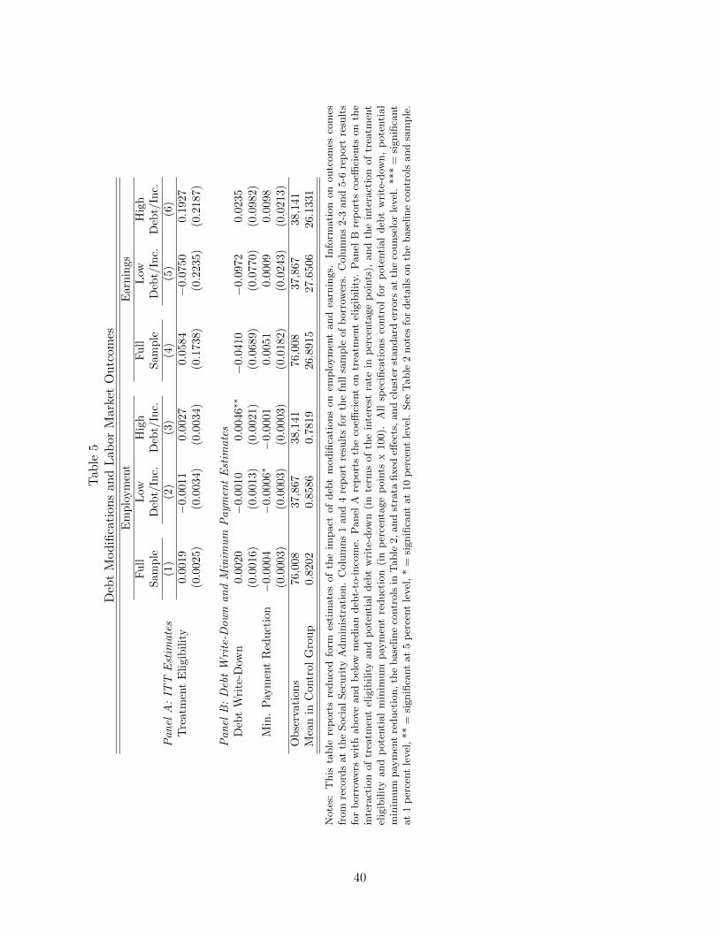
Tab

le5

Deb

tM

od

ifica

tion

san

dL

abor

Mar

ket

Ou

tcom

esE

mp

loym

ent

Earn

ings

Fu

llL

owH

igh

Fu

llL

owH

igh

Sam

ple

Deb

t/In

c.D

ebt/

Inc.

Sam

ple

Deb

t/In

c.D

ebt/

Inc.

Pan

elA

:IT

TE

stim

ate

s(1

)(2

)(3

)(4

)(5

)(6

)T

reat

men

tE

ligi

bil

ity

0.0019

−0.

0011

0.0027

0.0584

−0.

0750

0.1927

(0.0

025)

(0.0

034)

(0.0

034)

(0.1

738)

(0.2

235)

(0.2

187)

Pan

elB

:D

ebt

Wri

te-D

ow

nan

dM

inim

um

Paym

ent

Est

imate

sD

ebt

Wri

te-D

own

0.0020

−0.

0010

0.0046∗

∗−

0.0410

−0.

0972

0.0

235

(0.0

016)

(0.0

013)

(0.0

021)

(0.0

689)

(0.0

770)

(0.0

982)

Min

.P

aym

ent

Red

uct

ion−

0.0004

−0.

0006∗

−0.0

001

0.0051

0.00

09

0.0

098

(0.0

003)

(0.0

003)

(0.0

003)

(0.0

182)

(0.0

243)

(0.0

213)

Ob

serv

atio

ns

76,0

08

37,8

67

38,1

41

76,0

08

37,8

67

38,1

41

Mea

nin

Con

trol

Gro

up

0.8

202

0.8

586

0.7

819

26.8

915

27.6

506

26.1

331

Note

s:T

his

table

rep

ort

sre

duce

dfo

rmes

tim

ate

sof

the

impact

of

deb

tm

odifi

cati

ons

on

emplo

ym

ent

and

earn

ings.

Info

rmati

on

on

outc

om

esco

mes

from

reco

rds

at

the

Soci

al

Sec

uri

tyA

dm

inis

trati

on.

Colu

mns

1and

4re

port

resu

lts

for

the

full

sam

ple

of

borr

ower

s.C

olu

mns

2-3

and

5-6

rep

ort

resu

lts

for

borr

ower

sw

ith

ab

ove

and

bel

owm

edia

ndeb

t-to

-inco

me.

Panel

Are

port

sth

eco

effici

ent

on

trea

tmen

tel

igib

ilit

y.P

anel

Bre

port

sco

effici

ents

on

the

inte

ract

ion

of

trea

tmen

tel

igib

ilit

yand

pote

nti

al

deb

tw

rite

-dow

n(i

nte

rms

of

the

inte

rest

rate

inp

erce

nta

ge

poin

ts),

and

the

inte

ract

ion

of

trea

tmen

tel

igib

ilit

yand

pote

nti

al

min

imum

pay

men

tre

duct

ion

(in

per

centa

ge

poin

tsx

100).

All

spec

ifica

tions

contr

ol

for

pote

nti

al

deb

tw

rite

-dow

n,

pote

nti

al

min

imum

pay

men

tre

duct

ion,

the

base

line

contr

ols

inT

able

2,

and

stra

tafixed

effec

ts,

and

clust

erst

andard

erro

rsat

the

counse

lor

level

.***

=si

gnifi

cant

at

1p

erce

nt

level

,**

=si

gnifi

cant

at

5p

erce

nt

level

,*

=si

gnifi

cant

at

10

per

cent

level

.See

Table

2note

sfo

rdet

ails

on

the

base

line

contr

ols

and

sam

ple

.

40

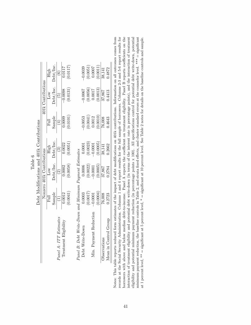
Tab

le6

Deb

tM

od

ifica

tion

san

d40

1kC

ontr

ibu

tion

sN

on

zero

401k

Contr

ibu

tion

s401k

Contr

ibu

tion

sF

ull

Low

Hig

hF

ull

Low

Hig

hS

am

ple

Deb

t/In

c.D

ebt/

Inc.

Sam

ple

Deb

t/In

c.D

ebt/

Inc.

Pan

elA

:IT

TE

stim

ate

s(1

)(2

)(3

)(4

)(5

)(6

)T

reat

men

tE

ligi

bil

ity

0.0012

0.0002

0.0022

0.0009

−0.0

098

0.0117

(0.0

041)

(0.0

058)

(0.0

051)

(0.0

101)

(0.0

131)

(0.0

117)

Pan

elB

:D

ebt

Wri

te-D

ow

nan

dM

inim

um

Paym

ent

Est

imate

sD

ebt

Wri

te-D

own

0.0003

0.0006

0.0001

−0.

0053

−0.

0067

−0.

0039

(0.0

017)

(0.0

022)

(0.0

023)

(0.0

041)

(0.0

056)

(0.0

051)

Min

.P

aym

ent

Red

uct

ion−

0.0001

−0.

0001

−0.0

001

0.0012

0.0017

0.0007

(0.0

004)

(0.0

005)

(0.0

005)

(0.0

010)

(0.0

013)

(0.0

011)

Ob

serv

atio

ns

76,0

08

37,8

67

38,1

41

76,0

08

37,8

67

38,1

41

Mea

nin

Con

trol

Gro

up

0.2

723

0.2

784

0.2

662

0.4

643

0.4

413

0.4

872

Note

s:T

his

table

rep

ort

sre

duce

dfo

rmes

tim

ate

sof

the

impact

of

deb

tm

odifi

cati

ons

on

401k

contr

ibuti

ons.

Info

rmati

on

on

all

outc

om

esco

mes

from

reco

rds

at

the

Soci

al

Sec

uri

tyA

dm

inis

trati

on.

Colu

mns

1and

4re

port

resu

lts

for

the

full

sam

ple

of

borr

ower

s.C

olu

mns

2-3

and

5-6

rep

ort

resu

lts

for

borr

ower

sw

ith

ab

ove

and

bel

owm

edia

ndeb

t-to

-inco

me.

Panel

Are

port

sth

eco

effici

ent

on

trea

tmen

tel

igib

ilit

y.P

anel

Bre

port

sco

effici

ents

on

the

inte

ract

ion

of

trea

tmen

tel

igib

ilit

yand

pote

nti

al

deb

tw

rite

-dow

n(i

nte

rms

of

the

inte

rest

rate

inp

erce

nta

ge

poin

ts),

and

the

inte

ract

ion

of

trea

tmen

tel

igib

ilit

yand

pote

nti

al

min

imum

pay

men

tre

duct

ion

(in

per

centa

ge

poin

tsx

100).

All

spec

ifica

tions

contr

ol

for

pote

nti

al

deb

tw

rite

-dow

n,

pote

nti

al

min

imum

pay

men

tre

duct

ion,

the

base

line

contr

ols

inT

able

2,

and

stra

tafixed

effec

ts,

and

clust

erst

andard

erro

rsat

the

counse

lor

level

.***

=si

gnifi

cant

at

1p

erce

nt

level

,**

=si

gnifi

cant

at

5p

erce

nt

level

,*

=si

gnifi

cant

at

10

per

cent

level

.See

Table

2note

sfo

rdet

ails

on

the

base

line

contr

ols

and

sam

ple

.

41

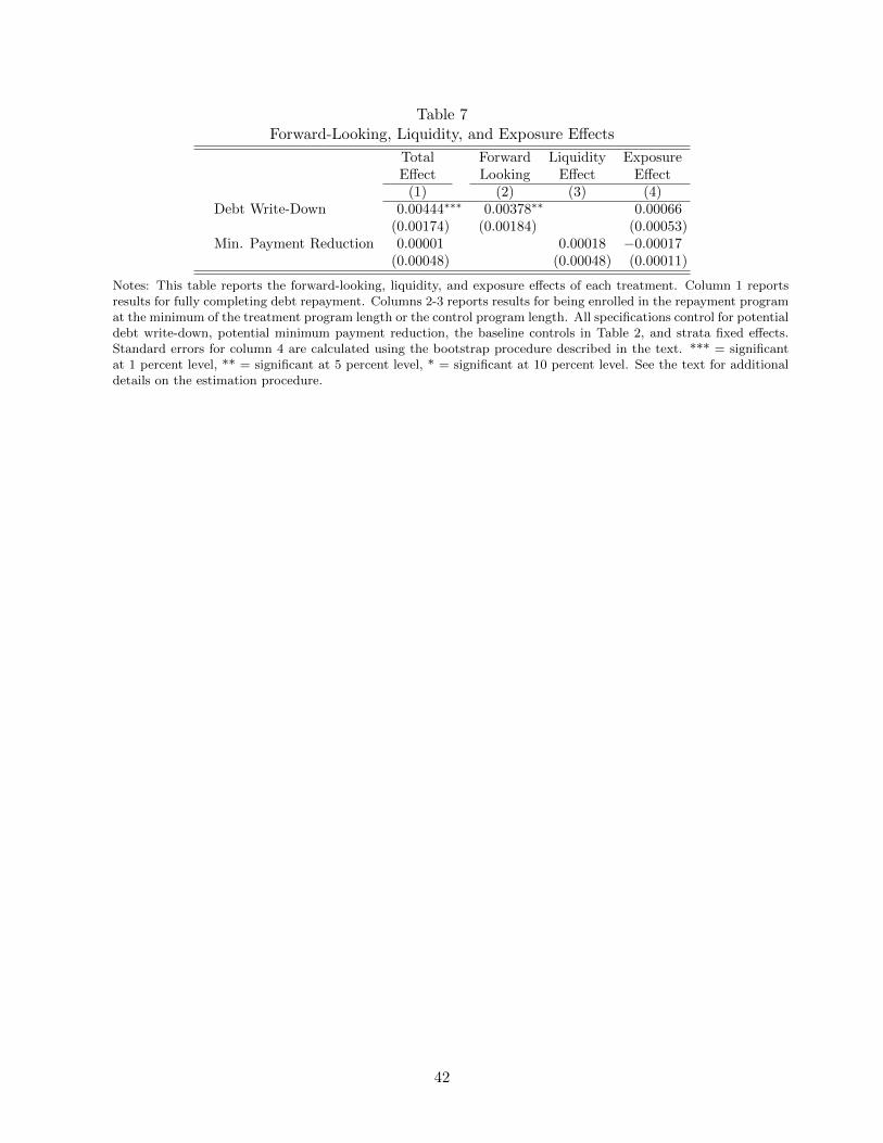
Table 7Forward-Looking, Liquidity, and Exposure Effects

Total Forward Liquidity ExposureEffect Looking Effect Effect

(1) (2) (3) (4)Debt Write-Down 0.00444∗∗∗ 0.00378∗∗ 0.00066

(0.00174) (0.00184) (0.00053)Min. Payment Reduction 0.00001 0.00018 −0.00017

(0.00048) (0.00048) (0.00011)

Notes: This table reports the forward-looking, liquidity, and exposure effects of each treatment. Column 1 reportsresults for fully completing debt repayment. Columns 2-3 reports results for being enrolled in the repayment programat the minimum of the treatment program length or the control program length. All specifications control for potentialdebt write-down, potential minimum payment reduction, the baseline controls in Table 2, and strata fixed effects.Standard errors for column 4 are calculated using the bootstrap procedure described in the text. *** = significantat 1 percent level, ** = significant at 5 percent level, * = significant at 10 percent level. See the text for additionaldetails on the estimation procedure.

42

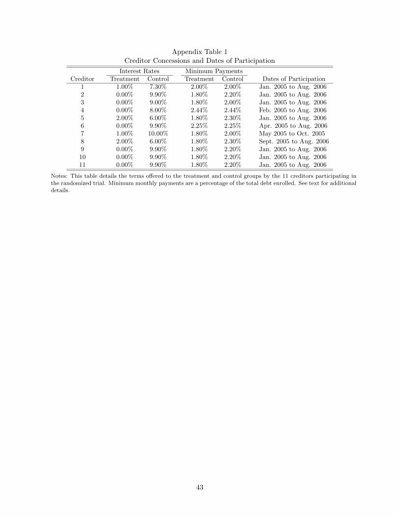
Appendix Table 1Creditor Concessions and Dates of Participation

Interest Rates Minimum PaymentsCreditor Treatment Control Treatment Control Dates of Participation

1 1.00% 7.30% 2.00% 2.00% Jan. 2005 to Aug. 20062 0.00% 9.90% 1.80% 2.20% Jan. 2005 to Aug. 20063 0.00% 9.00% 1.80% 2.00% Jan. 2005 to Aug. 20064 0.00% 8.00% 2.44% 2.44% Feb. 2005 to Aug. 20065 2.00% 6.00% 1.80% 2.30% Jan. 2005 to Aug. 20066 0.00% 9.90% 2.25% 2.25% Apr. 2005 to Aug. 20067 1.00% 10.00% 1.80% 2.00% May 2005 to Oct. 20058 2.00% 6.00% 1.80% 2.30% Sept. 2005 to Aug. 20069 0.00% 9.90% 1.80% 2.20% Jan. 2005 to Aug. 200610 0.00% 9.90% 1.80% 2.20% Jan. 2005 to Aug. 200611 0.00% 9.90% 1.80% 2.20% Jan. 2005 to Aug. 2006

Notes: This table details the terms offered to the treatment and control groups by the 11 creditors participating inthe randomized trial. Minimum monthly payments are a percentage of the total debt enrolled. See text for additionaldetails.

43

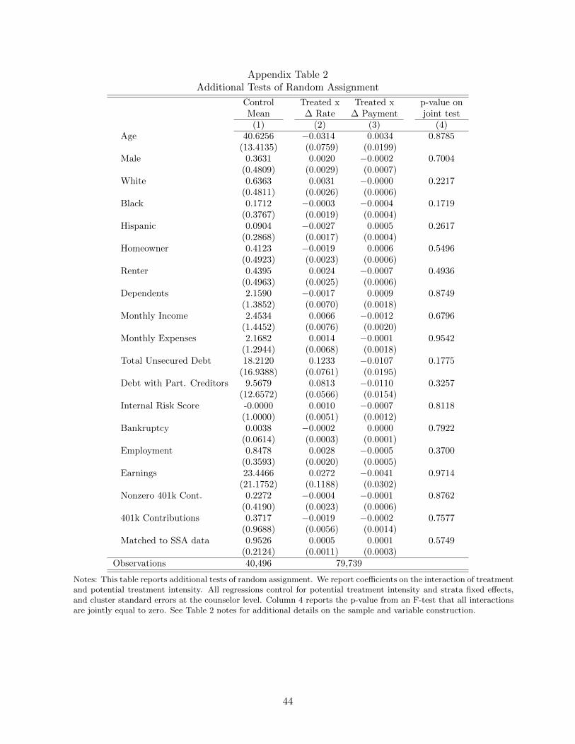
Appendix Table 2Additional Tests of Random Assignment

Control Treated x Treated x p-value onMean ∆ Rate ∆ Payment joint test

(1) (2) (3) (4)Age 40.6256 −0.0314 0.0034 0.8785

(13.4135) (0.0759) (0.0199)Male 0.3631 0.0020 −0.0002 0.7004

(0.4809) (0.0029) (0.0007)White 0.6363 0.0031 −0.0000 0.2217

(0.4811) (0.0026) (0.0006)Black 0.1712 −0.0003 −0.0004 0.1719

(0.3767) (0.0019) (0.0004)Hispanic 0.0904 −0.0027 0.0005 0.2617

(0.2868) (0.0017) (0.0004)Homeowner 0.4123 −0.0019 0.0006 0.5496

(0.4923) (0.0023) (0.0006)Renter 0.4395 0.0024 −0.0007 0.4936

(0.4963) (0.0025) (0.0006)Dependents 2.1590 −0.0017 0.0009 0.8749

(1.3852) (0.0070) (0.0018)Monthly Income 2.4534 0.0066 −0.0012 0.6796

(1.4452) (0.0076) (0.0020)Monthly Expenses 2.1682 0.0014 −0.0001 0.9542

(1.2944) (0.0068) (0.0018)Total Unsecured Debt 18.2120 0.1233 −0.0107 0.1775

(16.9388) (0.0761) (0.0195)Debt with Part. Creditors 9.5679 0.0813 −0.0110 0.3257

(12.6572) (0.0566) (0.0154)Internal Risk Score -0.0000 0.0010 −0.0007 0.8118

(1.0000) (0.0051) (0.0012)Bankruptcy 0.0038 −0.0002 0.0000 0.7922

(0.0614) (0.0003) (0.0001)Employment 0.8478 0.0028 −0.0005 0.3700

(0.3593) (0.0020) (0.0005)Earnings 23.4466 0.0272 −0.0041 0.9714

(21.1752) (0.1188) (0.0302)Nonzero 401k Cont. 0.2272 −0.0004 −0.0001 0.8762

(0.4190) (0.0023) (0.0006)401k Contributions 0.3717 −0.0019 −0.0002 0.7577

(0.9688) (0.0056) (0.0014)Matched to SSA data 0.9526 0.0005 0.0001 0.5749

(0.2124) (0.0011) (0.0003)Observations 40,496 79,739

Notes: This table reports additional tests of random assignment. We report coefficients on the interaction of treatmentand potential treatment intensity. All regressions control for potential treatment intensity and strata fixed effects,and cluster standard errors at the counselor level. Column 4 reports the p-value from an F-test that all interactionsare jointly equal to zero. See Table 2 notes for additional details on the sample and variable construction.

44

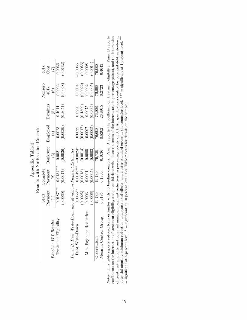
Ap

pen

dix

Tab

le3

Res

ult

sw

ith

No

Bas

elin

eC

ontr

ols

Sta

rtC

om

ple

teN

on

zero

401k

Pay

men

tP

aym

ent

Ban

kru

pt

Em

plo

yed

Earn

ings

401k

Cont.

Pan

elA

:IT

TR

esu

lts

(1)

(2)

(3)

(4)

(5)

(6)

(7)

Tre

atm

ent

Eli

gib

ilit

y0.0

187∗

∗∗0.0

134∗∗

∗−

0.0021

0.0023

0.1011

0.0002

−0.

0036

(0.0

060)

(0.0

047)

(0.0

036)

(0.0

039)

(0.3

057)

(0.0

048)

(0.0

132)

Pan

elB

:D

ebt

Wri

te-D

ow

nan

dM

inim

um

Paym

ent

Est

imate

sD

ebt

Wri

te-D

own

0.0

055∗

∗0.0

049∗∗

∗−

0.0024∗

0.0

022

0.0290

0.0004

−0.

0056

(0.0

025)

(0.0

018)

(0.0

014)

(0.0

017)

(0.1

309)

(0.0

022)

(0.0

056)

Min

.P

aym

ent

Red

uct

ion

0.0003

−0.

0001

0.0005

−0.0

007

−0.

0075

−0.

0002

0.0008

(0.0

006)

(0.0

005)

(0.0

003)

(0.0

005)

(0.0

334)

(0.0

005)

(0.0

014)

Ob

serv

atio

ns

79,7

39

79,7

39

79,7

39

76,0

08

76,0

08

76,0

08

76,0

08

Mea

nin

Con

trol

Gro

up

0.3

185

0.1

366

0.1

036

0.8

202

26.8

915

0.2723

0.4

643

Note

s:T

his

table

rep

ort

sre

duce

dfo

rmes

tim

ate

sw

ith

no

base

line

contr

ols

.P

anel

Are

port

sth

eco

effici

ent

on

trea

tmen

tel

igib

ilit

y.P

anel

Bre

port

sco

effici

ents

on

the

inte

ract

ion

of

trea

tmen

tel

igib

ilit

yand

pote

nti

aldeb

tw

rite

-dow

n(i

nte

rms

of

the

inte

rest

rate

inp

erce

nta

ge

poin

ts),

and

the

inte

ract

ion

of

trea

tmen

tel

igib

ilit

yand

pote

nti

al

min

imum

pay

men

tre

duct

ion

(in

per

centa

ge

poin

tsx

100).

All

spec

ifica

tions

contr

ol

for

pote

nti

al

deb

tw

rite

-dow

n,

pote

nti

al

month

lym

inim

um

reduct

ion,

and

stra

tafixed

effec

ts,

and

clust

erst

andard

erro

rsat

the

counse

lor

level

.***

=si

gnifi

cant

at

1p

erce

nt

level

,**

=si

gnifi

cant

at

5p

erce

nt

level

,*

=si

gnifi

cant

at

10

per

cent

level

.See

Table

2note

sfo

rdet

ails

on

the

sam

ple

.

45

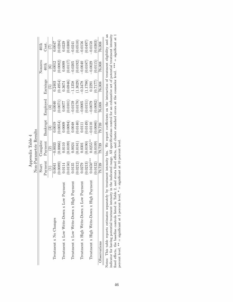
Ap

pen

dix

Tab

le4

Non

-Par

amet

ric

Res

ult

sS

tart

Com

ple

teN

on

zero

401k

Pay

men

tP

aym

ent

Ban

kru

pt

Em

plo

yed

Earn

ings

401k

Cont.

(1)

(2)

(3)

(4)

(5)

(6)

(7)

Tre

atm

ent

xN

oC

han

ges

0.0

041

−0.

0033

0.0019

0.0040

0.2403

0.0012

0.0047

(0.0

089)

(0.0

066)

(0.0

054)

(0.0

071)

(0.4

954)

(0.0

082)

(0.0

204)

Tre

atm

ent

xL

owW

rite

-Dow

nx

Low

Pay

men

t0.0

114

0.0110

0.0009

0.0077

0.3674

0.0099

0.0229

(0.0

150)

(0.0

109)

(0.0

094)

(0.0

101)

(0.6

946)

(0.0

117)

(0.0

300)

Tre

atm

ent

xL

owW

rite

-Dow

nx

Hig

hP

aym

ent

0.0

135

0.0024

0.0048

−0.0

159

−1.

1358

−0.

0205

−0.0

241

(0.0

212)

(0.0

181)

(0.0

140)

(0.0

178)

(1.3

029)

(0.0

192)

(0.0

510)

Tre

atm

ent

xH

igh

Wri

te-D

own

xL

owP

aym

ent

0.0

279

0.0301

0.0111

−0.0

005

−0.

3478

−0.

0040

−0.0

156

(0.0

213)

(0.0

190)

(0.0

149)

(0.0

151)

(1.1

798)

(0.0

187)

(0.0

497)

Tre

atm

ent

xH

igh

Wri

te-D

own

xH

igh

Pay

men

t0.

0450∗

∗∗0.

0255∗∗−

0.0110

−0.0

079

0.2291

−0.

0029

−0.0

158

(0.0

132)

(0.0

109)

(0.0

080)

(0.0

092)

(0.7

177)

(0.0

115)

(0.0

303)

Ob

serv

atio

ns

79,7

39

79,7

39

79,7

39

76,0

08

76,

008

76,0

08

76,0

08

Note

s:T

his

table

rep

ort

ses

tim

ate

sse

para

tely

by

trea

tmen

tin

tensi

tybin

.W

ere

port

coeffi

cien

tson

the

inte

ract

ion

of

trea

tmen

tel

igib

ilit

yand

an

indic

ato

rfo

rhav

ing

pote

nti

al

trea

tmen

tin

tensi

tyin

the

indic

ate

dra

nge.

All

spec

ifica

tions

contr

ol

for

an

exhaust

ive

set

of

pote

nti

al

trea

tmen

tin

tensi

tyfixed

effec

ts,

the

base

line

contr

ols

list

edin

Table

2,

and

stra

tafixed

effec

ts,

and

clust

erst

andard

erro

rsat

the

counse

lor

level

.***

=si

gnifi

cant

at

1p

erce

nt

level

,**

=si

gnifi

cant

at

5p

erce

nt

level

,*

=si

gnifi

cant

at

10

per

cent

level

.

46

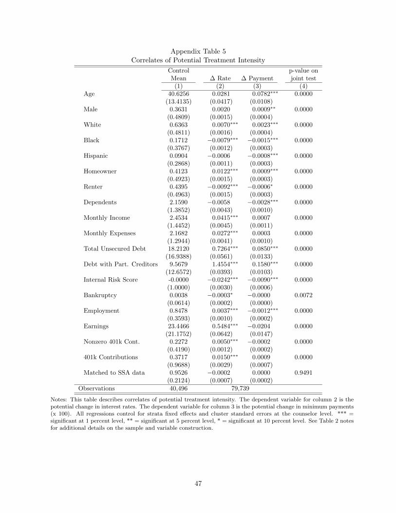
Appendix Table 5Correlates of Potential Treatment Intensity

Control p-value onMean ∆ Rate ∆ Payment joint test

(1) (2) (3) (4)Age 40.6256 0.0281 0.0782∗∗∗ 0.0000

(13.4135) (0.0417) (0.0108)Male 0.3631 0.0020 0.0009∗∗ 0.0000

(0.4809) (0.0015) (0.0004)White 0.6363 0.0070∗∗∗ 0.0023∗∗∗ 0.0000

(0.4811) (0.0016) (0.0004)Black 0.1712 −0.0079∗∗∗ −0.0015∗∗∗ 0.0000

(0.3767) (0.0012) (0.0003)Hispanic 0.0904 −0.0006 −0.0008∗∗∗ 0.0000

(0.2868) (0.0011) (0.0003)Homeowner 0.4123 0.0122∗∗∗ 0.0009∗∗∗ 0.0000

(0.4923) (0.0015) (0.0003)Renter 0.4395 −0.0092∗∗∗ −0.0006∗ 0.0000

(0.4963) (0.0015) (0.0003)Dependents 2.1590 −0.0058 −0.0028∗∗∗ 0.0000

(1.3852) (0.0043) (0.0010)Monthly Income 2.4534 0.0415∗∗∗ 0.0007 0.0000

(1.4452) (0.0045) (0.0011)Monthly Expenses 2.1682 0.0272∗∗∗ 0.0003 0.0000

(1.2944) (0.0041) (0.0010)Total Unsecured Debt 18.2120 0.7264∗∗∗ 0.0850∗∗∗ 0.0000

(16.9388) (0.0561) (0.0133)Debt with Part. Creditors 9.5679 1.4554∗∗∗ 0.1580∗∗∗ 0.0000

(12.6572) (0.0393) (0.0103)Internal Risk Score -0.0000 −0.0242∗∗∗ −0.0090∗∗∗ 0.0000

(1.0000) (0.0030) (0.0006)Bankruptcy 0.0038 −0.0003∗ −0.0000 0.0072

(0.0614) (0.0002) (0.0000)Employment 0.8478 0.0037∗∗∗ −0.0012∗∗∗ 0.0000

(0.3593) (0.0010) (0.0002)Earnings 23.4466 0.5484∗∗∗ −0.0204 0.0000

(21.1752) (0.0642) (0.0147)Nonzero 401k Cont. 0.2272 0.0050∗∗∗ −0.0002 0.0000

(0.4190) (0.0012) (0.0002)401k Contributions 0.3717 0.0150∗∗∗ 0.0009 0.0000

(0.9688) (0.0029) (0.0007)Matched to SSA data 0.9526 −0.0002 0.0000 0.9491

(0.2124) (0.0007) (0.0002)Observations 40,496 79,739

Notes: This table describes correlates of potential treatment intensity. The dependent variable for column 2 is thepotential change in interest rates. The dependent variable for column 3 is the potential change in minimum payments(x 100). All regressions control for strata fixed effects and cluster standard errors at the counselor level. *** =significant at 1 percent level, ** = significant at 5 percent level, * = significant at 10 percent level. See Table 2 notesfor additional details on the sample and variable construction.

47

Ap

pen

dix

Tab

le6

Ove

r-Id

enti

fica

tion

Tes

tsS

tart

Com

ple

teN

on

zero

401k

Pay

men

tP

aym

ent

Ban

kru

pt

Em

plo

yed

Earn

ings

401k

Cont.

(1)

(2)

(3)

(4)

(5)

(6)

(7)

Tre

atm

ent

xD

ebt

wit

hC

red

itor

1−

0.0

082

0.0128

0.0011

0.0040

0.0913

0.0155

0.0551

(0.0

220)

(0.0

184)

(0.0

149)

(0.0

112)

(0.6

054)

(0.0

163)

(0.0

413)

Tre

atm

ent

xD

ebt

wit

hC

red

itor

2−

0.0

011

−0.0

067

0.0040

0.0041

0.6825

0.0141

0.0364

(0.0

145)

(0.0

120)

(0.0

114)

(0.0

069)

(0.4

672)

(0.0

114)

(0.0

293)

Tre

atm

ent

xD

ebt

wit

hC

red

itor

30.0

009

0.0014

−0.

0069

0.0039

−0.

0077

0.0009

0.0257

(0.0

153)

(0.0

126)

(0.0

109)

(0.0

081)

(0.5

065)

(0.0

114)

(0.0

256)

Tre

atm

ent

xD

ebt

wit

hC

red

itor

4−

0.0

532

−0.

2493

0.0422

−0.0

856

−2.

0041

−0.

1251

0.0978

(0.2

299)

(0.2

190)

(0.1

059)

(0.1

483)

(9.5

178)

(0.1

771)

(0.3

886)

Tre

atm

ent

xD

ebt

wit

hC

red

itor

50.0

005

−0.

0062

0.0159

−0.0

059

−0.

9102

0.0223

0.0393

(0.0

238)

(0.0

173)

(0.0

163)

(0.0

142)

(0.9

091)

(0.0

188)

(0.0

486)

Tre

atm

ent

xD

ebt

wit

hC

red

itor

60.0

049

0.0074

−0.

0038

0.0059

0.1850

0.0028

0.0117

(0.0

142)

(0.0

113)

(0.0

093)

(0.0

067)

(0.3

983)

(0.0

099)

(0.0

242)

Tre

atm

ent

xD

ebt

wit

hC

red

itor

70.0

500∗

∗∗0.

0339∗∗

∗0.

0098

0.0063

0.9332

0.0083

0.0321

(0.0

162)

(0.0

125)

(0.0

123)

(0.0

100)

(0.6

737)

(0.0

145)

(0.0

366)

Tre

atm

ent

xD

ebt

wit

hC

red

itor

8−

0.0

086

−0.

0097

0.0030

−0.0

050

−0.

4827

−0.

0068

−0.0

244

(0.0

124)

(0.0

104)

(0.0

084)

(0.0

062)

(0.3

562)

(0.0

082)

(0.0

241)

Tre

atm

ent

xD

ebt

wit

hC

red

itor

9−

0.0

063

0.0014

0.0025

0.0047

0.2154

−0.

0044

0.0033

(0.0

114)

(0.0

095)

(0.0

083)

(0.0

061)

(0.3

667)

(0.0

090)

(0.0

196)

Tre

atm

ent

xD

ebt

wit

hC

red

itor

10−

0.0

036

0.0080

0.0055

0.0067

0.4029

0.0002

0.0022

(0.0

134)

(0.0

111)

(0.0

091)

(0.0

071)

(0.4

866)

(0.0

115)

(0.0

274)

Tre

atm

ent

xD

ebt

wit

hC

red

itor

11−

0.0

152

0.0055

0.0040

−0.0

018

−0.

0410

0.0037

0.0168

(0.0

258)

(0.0

238)

(0.0

165)

(0.0

123)

(0.9

303)

(0.0

213)

(0.0

561)

p-v

alu

efr

omjo

int

F-t

est

0.4

16

0.3

69

0.9

86

0.9

40

0.7

18

0.8

40

0.8

34

Ob

serv

atio

ns

79,7

39

79,7

39

79,7

39

76,0

08

76,0

08

76,0

08

76,0

08

Note

s:T

his

table

rep

ort

sov

er-i

den

tifica

tion

test

s.W

ere

port

the

coeffi

cien

ton

trea

tmen

tel

igib

ilit

yin

tera

cted

wit

han

indic

ato

rfo

rhav

ing

deb

tw

ith

each

cred

itca

rdbank.

We

als

ore

port

the

p-v

alu

efr

om

an

F-t

est

that

all

inte

ract

ions

ina

colu

mn

are

join

tly

equal

toze

ro.

All

spec

ifica

tions

contr

ol

for

trea

tmen

tel

igib

ilit

yin

tera

cted

wit

hth

ep

ote

nti

al

deb

tw

rite

-dow

n,

trea

tmen

tel

igib

ilit

yin

tera

cted

wit

hth

ep

ote

nti

al

min

imum

pay

men

tre

duct

ion,

pote

nti

al

deb

tw

rite

-dow

n,

pote

nti

al

min

imum

pay

men

tre

duct

ion,

the

base

line

contr

ols

list

edin

Table

2,

and

stra

tafixed

effec

ts.

Sta

ndard

erro

rsare

clust

ered

at

the

counse

lor

level

.***

=si

gnifi

cant

at

1p

erce

nt

level

,**

=si

gnifi

cant

at

5p

erce

nt

level

,*

=si

gnifi

cant

at

10

per

cent

level

.See

Table

2note

sfo

rdet

ails

on

the

base

line

contr

ols

and

sam

ple

.

48

Ap

pen

dix

Tab

le7

Res

ult

sby

Gen

der

Sta

rtC

om

ple

teN

on

zero

401k

Pay

men

tP

aym

ent

Ban

kru

pt

Em

plo

yed

Earn

ings

401k

Cont.

Pan

elA

:IT

TE

stim

ate

s(1

)(2

)(3

)(4

)(5

)(6

)(7

)(1

)T

reat

men

tx

Mal

e0.0

149

0.0095

−0.

0040

−0.

0033

0.1720

0.0002

0.0093

(0.0

101)

(0.0

077)

(0.0

069)

(0.0

062)

(0.5

275)

(0.0

085)

(0.0

233)

(2)

Tre

atm

ent

xF

emal

e0.

0226∗∗

∗0.

0165∗

∗∗−

0.0012

0.0054

−0.

0386

0.0001

−0.0

129

(0.0

075)

(0.0

060)

(0.0

049)

(0.0

051)

(0.3

358)

(0.0

060)

(0.0

156)

p-v

alu

efo

r(1

)-(2

)[0.5

219]

[0.4

660]

[0.7

484]

[0.2

887]

[0.7

272]

[0.9

906]

[0.4

287]

Pan

elB

:D

ebt

Wri

te-D

ow

nan

dM

inim

um

Paym

ent

(3)

Wri

te-D

own

xM

ale

0.0

016

0.0002

−0.

0013

0.0031

0.0660

0.0002

−0.0

072

(0.0

034)

(0.0

025)

(0.0

022)

(0.0

025)

(0.1

890)

(0.0

028)

(0.0

077)

(4)

Wri

te-D

own

xF

emal

e0.0

081∗

∗∗0.

0074∗∗

∗−

0.0033∗

∗0.0

017

−0.

0180

0.0006

−0.0

050

(0.0

030)

(0.0

024)

(0.0

017)

(0.0

020)

(0.1

305)

(0.0

026)

(0.0

066)

p-v

alu

efo

r(3

)-(4

)[0.0

935]

[0.0

271]

[0.3

981]

[0.6

105]

[0.6

510]

[0.9

073]

[0.8

068]

(5)

Pay

men

tx

Mal

e0.0

013

0.0004

0.0004

−0.0

006

−0.

0133

−0.

0006

0.0003

(0.0

009)

(0.0

006)

(0.0

005)

(0.0

007)

(0.0

456)

(0.0

007)

(0.0

020)

(6)

Pay

men

tx

Fem

ale

−0.0

002

−0.

0001

0.0005

−0.0

008

−0.

0014

−0.

0000

0.0012

(0.0

008)

(0.0

006)

(0.0

004)

(0.0

005)

(0.0

351)

(0.0

006)

(0.0

016)

p-v

alu

efo

r(5

)-(6

)[0.1

486]

[0.5

660]

[0.7

995]

[0.8

779]

[0.7

997]

[0.4

941]

[0.6

733]

Ob

serv

atio

ns

79,7

39

79,7

39

79,7

39

76,0

08

76,0

08

76,0

08

76,0

08

Mea

nif

Mal

e0.3

121

0.1

255

0.1

252

0.8

430

32.0

416

0.2

825

0.5

633

Mea

nif

Fem

ale

0.3

203

0.1

391

0.0

993

0.8

073

23.9

590

0.2

666

0.4

079

Note

s:T

his

table

rep

ort

sre

sult

sby

gen

der

.P

anel

Are

port

sco

effici

ents

on

the

inte

ract

ion

of

gen

der

xtr

eatm

ent

elig

ibilit

y.P

anel

Bre

port

sco

effici

ents

on

the

inte

ract

ion

of

gen

der

xtr

eatm

ent

elig

ibilit

yx

pote

nti

al

trea

tmen

tin

tensi

ty.

All

spec

ifica

tions

contr

ol

for

an

indic

ato

rfo

rp

ote

nti

al

trea

tmen

tin

tensi

ty,

the

base

line

vari

able

slist

edin

Table

2,

and

stra

tafixed

effec

ts.

Sta

ndard

erro

rsare

clust

ered

at

the

counse

lor

level

.***

=si

gnifi

cant

at

1p

erce

nt

level

,**

=si

gnifi

cant

at

5p

erce

nt

level

,*

=si

gnifi

cant

at

10

per

cent

level

.See

Table

2note

sfo

rdet

ails

on

the

base

line

contr

ols

and

sam

ple

.

49

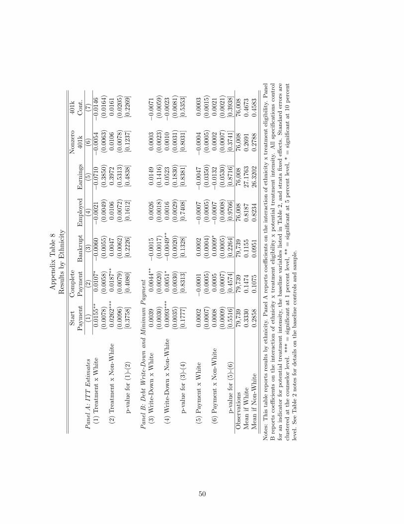
Ap

pen

dix

Tab

le8

Res

ult

sby

Eth

nic

ity

Sta

rtC

om

ple

teN

on

zero

401k

Pay

men

tP

aym

ent

Ban

kru

pt

Em

plo

yed

Earn

ings

401k

Cont.

Pan

elA

:IT

TE

stim

ate

s(1

)(2

)(3

)(4

)(5

)(6

)(7

)(1

)T

reat

men

tx

Wh

ite

0.0

155∗

∗0.

0107∗−

0.0060

−0.0

021

−0.

0710

−0.

0054

−0.0

146

(0.0

078)

(0.0

058)

(0.0

055)

(0.0

049)

(0.3

850)

(0.0

063)

(0.0

164)

(2)

Tre

atm

ent

xN

on-W

hit

e0.0

262∗

∗∗0.

0187∗∗

0.0047

0.0106

0.3972

0.0106

0.0161

(0.0

096)

(0.0

079)

(0.0

062)

(0.0

072)

(0.5

313)

(0.0

078)

(0.0

205)

p-v

alu

efo

r(1

)-(2

)[0.3

758]

[0.4

080]

[0.2

226]

[0.1

612]

[0.4

838]

[0.1

237]

[0.2

269]

Pan

elB

:D

ebt

Wri

te-D

ow

nan

dM

inim

um

Paym

ent

(3)

Wri

te-D

own

xW

hit

e0.0

039

0.0044∗∗−

0.0015

0.0026

0.0149

0.0003

−0.0

071

(0.0

030)

(0.0

020)

(0.0

017)

(0.0

018)

(0.1

416)

(0.0

023)

(0.0

059)

(4)

Wri

te-D

own

xN

on-W

hit

e0.0

093∗

∗∗0.

0051∗−

0.0049∗

∗0.0

016

0.0523

0.0010

−0.0

023

(0.0

035)

(0.0

030)

(0.0

020)

(0.0

029)

(0.1

830)

(0.0

031)

(0.0

081)

p-v

alu

efo

r(3

)-(4

)[0.1

777]

[0.8

313]

[0.1

328]

[0.7

408]

[0.8

381]

[0.8

031]

[0.5

353]

(5)

Pay

men

tx

Wh

ite

0.0

002

−0.

0001

0.0002

−0.0

007

−0.

0047

−0.

0004

0.0003

(0.0

007)

(0.0

005)

(0.0

004)

(0.0

005)

(0.0

350)

(0.0

005)

(0.0

015)

(6)

Pay

men

tx

Non

-Wh

ite

0.0

008

0.0005

0.0009∗

−0.0

007

−0.

0132

0.0002

0.0021

(0.0

009)

(0.0

007)

(0.0

005)

(0.0

008)

(0.0

530)

(0.0

007)

(0.0

021)

p-v

alu

efo

r(5

)-(6

)[0.5

516]

[0.4

574]

[0.2

264]

[0.9

766]

[0.8

716]

[0.3

741]

[0.3

938]

Ob

serv

atio

ns

79,7

39

79,7

39

79,7

39

76,0

08

76,0

08

76,0

08

76,0

08

Mea

nif

Wh

ite

0.3

330

0.1

474

0.1

155

0.8

187

27.1

763

0.2

691

0.4

673

Mea

nif

Non

-Wh

ite

0.2

858

0.1

075

0.0

951

0.8

234

26.3

202

0.2

788

0.4

583

Note

s:T

his

table

rep

ort

sre

sult

sby

ethnic

ity.

Panel

Are

port

sco

effici

ents

on

the

inte

ract

ion

of

ethnic

ity

xtr

eatm

ent

elig

ibilit

y.P

anel

Bre

port

sco

effici

ents

on

the

inte

ract

ion

of

ethnic

ity

xtr

eatm

ent

elig

ibilit

yx

pote

nti

al

trea

tmen

tin

tensi

ty.

All

spec

ifica

tions

contr

ol

for

an

indic

ato

rfo

rp

ote

nti

al

trea

tmen

tin

tensi

ty,

the

base

line

vari

able

slist

edin

Table

2,

and

stra

tafixed

effec

ts.

Sta

ndard

erro

rsare

clust

ered

at

the

counse

lor

level

.***

=si

gnifi

cant

at

1p

erce

nt

level

,**

=si

gnifi

cant

at

5p

erce

nt

level

,*

=si

gnifi

cant

at

10

per

cent

level

.See

Table

2note

sfo

rdet

ails

on

the

base

line

contr

ols

and

sam

ple

.

50

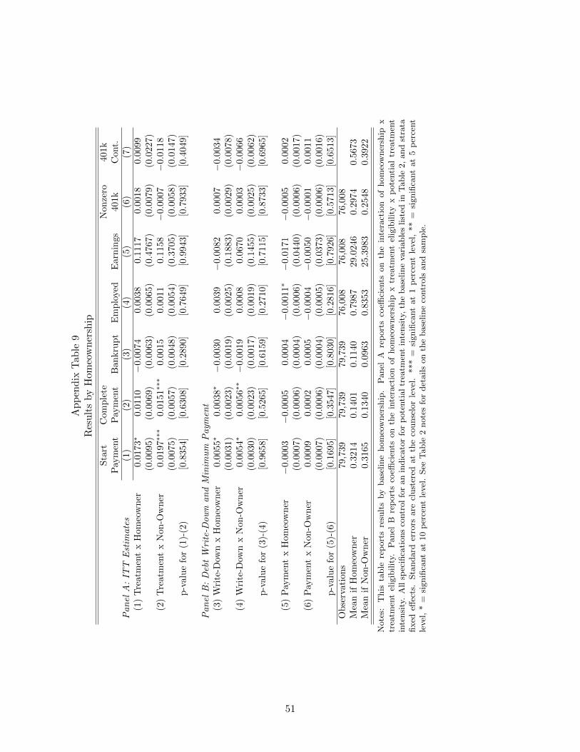
Ap

pen

dix

Tab

le9

Res

ult

sby

Hom

eow

ner

ship

Sta

rtC

om

ple

teN

on

zero

401k

Pay

men

tP

aym

ent

Ban

kru

pt

Em

plo

yed

Earn

ings

401k

Cont.

Pan

elA

:IT

TE

stim

ate

s(1

)(2

)(3

)(4

)(5

)(6

)(7

)(1

)T

reat

men

tx

Hom

eow

ner

0.0

173∗

0.0110

−0.0

074

0.0038

0.1117

0.0018

0.0099

(0.0

095)

(0.0

069)

(0.0

063)

(0.0

065)

(0.4

767)

(0.0

079)

(0.0

227)

(2)

Tre

atm

ent

xN

on-O

wn

er0.0

197∗∗

∗0.

0151∗

∗∗0.0

015

0.0011

0.1158

−0.0

007

−0.

0118

(0.0

075)

(0.0

057)

(0.0

048)

(0.0

054)

(0.3

705)

(0.0

058)

(0.0

147)

p-v

alu

efo

r(1

)-(2

)[0.8

354]

[0.6

308]

[0.2

890]

[0.7

649]

[0.9

943]

[0.7

933]

[0.4

049]

Pan

elB

:D

ebt

Wri

te-D

ow

nan

dM

inim

um

Paym

ent

(3)

Wri

te-D

own

xH

omeo

wn

er0.

0055∗

0.0038∗

−0.

0030

0.0039

−0.

0082

0.0007

−0.

0034

(0.0

031)

(0.0

023)

(0.0

019)

(0.0

025)

(0.1

883)

(0.0

029)

(0.0

078)

(4)

Wri

te-D

own

xN

on-O

wn

er0.

0054∗

0.0056∗

∗−

0.0019

0.0008

0.0670

0.0003

−0.0

066

(0.0

030)

(0.0

023)

(0.0

017)

(0.0

019)

(0.1

455)

(0.0

025)

(0.0

062)

p-v

alu

efo

r(3

)-(4

)[0.9

658]

[0.5

265]

[0.6

159]

[0.2

710]

[0.7

115]

[0.8

733]

[0.6

965]

(5)

Pay

men

tx

Hom

eow

ner

−0.0

003

−0.

0005

0.0004

−0.0

011∗

−0.

0171

−0.

0005

0.0002

(0.0

007)

(0.0

006)

(0.0

004)

(0.0

006)

(0.0

440)

(0.0

006)

(0.0

017)

(6)

Pay

men

tx

Non

-Ow

ner

0.0009

0.0002

0.0005

−0.0

004

−0.

0050

−0.

0001

0.0011

(0.0

007)

(0.0

006)

(0.0

004)

(0.0

005)

(0.0

373)

(0.0

006)

(0.0

016)

p-v

alu

efo

r(5

)-(6

)[0.1

695]

[0.3

547]

[0.8

030]

[0.2

816]

[0.7

926]

[0.5

713]

[0.6

513]

Ob

serv

atio

ns

79,7

39

79,7

39

79,7

39

76,0

08

76,0

08

76,0

08

Mea

nif

Hom

eow

ner

0.3

214

0.1

401

0.1

140

0.7

987

29.0

246

0.2

974

0.5

673

Mea

nif

Non

-Ow

ner

0.3

165

0.1

340

0.0

963

0.8

353

25.3

983

0.2

548

0.3

922

Note

s:T

his

table

rep

ort

sre

sult

sby

base

line

hom

eow

ner

ship

.P

anel

Are

port

sco

effici

ents

on

the

inte

ract

ion

of

hom

eow

ner

ship

xtr

eatm

ent

elig

ibilit

y.P

anel

Bre

port

sco

effici

ents

on

the

inte

ract

ion

of

hom

eow

ner

ship

xtr

eatm

ent

elig

ibilit

yx

pote

nti

al

trea

tmen

tin

tensi

ty.

All

spec

ifica

tions

contr

ol

for

an

indic

ato

rfo

rp

ote

nti

al

trea

tmen

tin

tensi

ty,

the

base

line

vari

able

slist

edin

Table

2,

and

stra

tafixed

effec

ts.

Sta

ndard

erro

rsare

clust

ered

at

the

counse

lor

level

.***

=si

gnifi

cant

at

1p

erce

nt

level

,**

=si

gnifi

cant

at

5p

erce

nt

level

,*

=si

gnifi

cant

at

10

per

cent

level

.See

Table

2note

sfo

rdet

ails

on

the

base

line

contr

ols

and

sam

ple

.

51

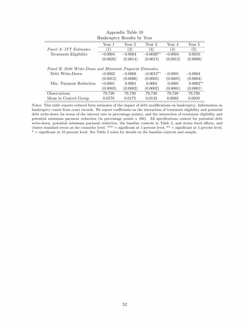
Appendix Table 10Bankruptcy Results by Year

Year 1 Year 2 Year 3 Year 4 Year 5Panel A: ITT Estimates (1) (2) (3) (4) (5)

Treatment Eligibility −0.0004 −0.0004 −0.0030∗∗ −0.0004 0.0010(0.0028) (0.0014) (0.0013) (0.0012) (0.0009)

Panel B: Debt Write-Down and Minimum Payment EstimatesDebt Write-Down −0.0002 −0.0008 −0.0012∗∗ −0.0001 −0.0004

(0.0012) (0.0006) (0.0005) (0.0005) (0.0004)Min. Payment Reduction −0.0001 0.0001 0.0001 0.0001 0.0002∗∗

(0.0003) (0.0002) (0.0002) (0.0001) (0.0001)Observations 79,739 79,739 79,739 79,739 79,739Mean in Control Group 0.0578 0.0173 0.0133 0.0093 0.0059

Notes: This table reports reduced form estimates of the impact of debt modifications on bankruptcy. Information onbankruptcy comes from court records. We report coefficients on the interaction of treatment eligibility and potentialdebt write-down (in terms of the interest rate in percentage points), and the interaction of treatment eligibility andpotential minimum payment reduction (in percentage points x 100). All specifications control for potential debtwrite-down, potential minimum payment reduction, the baseline controls in Table 2, and strata fixed effects, andcluster standard errors at the counselor level. *** = significant at 1 percent level, ** = significant at 5 percent level,* = significant at 10 percent level. See Table 2 notes for details on the baseline controls and sample.

52

Ap

pen

dix

Tab

le11

Pre

-BA

PC

PA

vs.

Pos

t-B

AP

CP

AS

tart

Com

ple

teN

on

zero

401k

Pay

men

tP

aym

ent

Ban

kru

pt

Em

plo

yed

Earn

ings

401k

Cont.

Pan

elA

:IT

TE

stim

ate

s(1

)(2

)(3

)(4

)(5

)(6

)(7

)(1

)T

reat

men

tx

Pre

-BA

PC

PA

0.0200∗∗

∗0.

0145∗

∗∗−

0.0

050

0.0065

0.1904

0.0001

−0.

0044

(0.0

073)

(0.0

056)

(0.0

046)

(0.0

046)

(0.3

491)

(0.0

056)

(0.0

154)

(2)

Tre

atm

ent

xP

ost-

BA

PC

PA

0.0151

0.0104

0.0066

−0.

0103

−0.

1750

0.0003

−0.

0013

(0.0

121)

(0.0

095)

(0.0

063)

(0.0

091)

(0.5

898)

(0.0

098)

(0.0

256)

p-v

alu

efo

r(1

)-(2

)[0.7

392]

[0.7

191]

[0.1

536]

[0.1

232]

[0.5

884]

[0.9

872]

[0.9

166]

Pan

elB

:D

ebt

Wri

te-D

ow

nan

dM

inim

um

Paym

ent

(3)

Wri

te-D

own

xP

re-B

AP

CP

A0.

0060∗∗

0.0059∗

∗∗−

0.0

031∗

0.0016

0.1094

0.0013

−0.

0029

(0.0

026)

(0.0

021)

(0.0

016)

(0.0

019)

(0.1

408)

(0.0

024)

(0.0

063)

(4)

Wri

te-D

own

xP

ost-

BA

PC

PA

0.0093∗∗

0.0060∗

−0.0

009

0.0031

−0.

1380

−0.0

014

−0.

0104

(0.0

039)

(0.0

031)

(0.0

018)

(0.0

026)

(0.1

913)

(0.0

033)

(0.0

082)

p-v

alu

efo

r(3

)-(4

)[0.3

738]

[0.9

686]

[0.3

253]

[0.5

805]

[0.1

929]

[0.4

357]

[0.3

908]

(5)

Pay

men

tx

Pre

-BA

PC

PA

−0.

0013∗−

0.0014∗

∗0.0

007

−0.

0004

−0.

0335

−0.0

005

−0.

0003

(0.0

007)

(0.0

005)

(0.0

004)

(0.0

005)

(0.0

379)

(0.0

006)

(0.0

016)

(6)

Pay

men

tx

Pos

t-B

AP

CP

A0.

0021∗∗

∗0.

0014∗

∗0.0

001

−0.

0012∗

0.0343

0.0002

0.0025

(0.0

008)

(0.0

007)

(0.0

004)

(0.0

006)

(0.0

433)

(0.0

007)

(0.0

017)

p-v

alu

efo

r(5

)-(6

)[0.0

001]

[0.0

003]

[0.2

369]

[0.2

702]

[0.1

336]

[0.3

114]

[0.1

554]

Ob

serv

atio

ns

79,7

39

79,7

39

79,7

39

76,0

08

76,0

08

76,0

08

76,0

08

Mea

nif

Pre

-BA

PC

PA

0.2

828

0.1

197

0.1

121

0.8

212

26.6

588

0.2

692

0.4

587

Mea

nif

Pos

t-B

AP

CP

A0.3

821

0.1

665

0.0

886

0.8

186

27.3

045

0.2

780

0.4

742

Note

s:T

his

table

rep

ort

sre

sult

sby

date

of

the

counse

ling

sess

ion.

Panel

Are

port

sco

effici

ents

on

the

inte

ract

ion

of

conta

ctin

gM

MI

bef

ore

or

aft

erth

eim

ple

men

tati

on

of

BA

PC

PA

(Oct

ob

er17,2005)

xtr

eatm

ent

elig

ibilit

y.P

anel

Bre

port

sco

effici

ents

on

the

inte

ract

ion

of

conta

ctin

gM

MI

bef

ore

or

aft

erth

eim

ple

men

tati

on

of

BA

PC

PA

(Oct

ob

er17,

2005)

xtr

eatm

ent

elig

ibilit

yx

pote

nti

al

trea

tmen

tin

tensi

ty.

All

spec

ifica

tions

contr

ol

for

an

indic

ato

rfo

rp

ote

nti

al

trea

tmen

tin

tensi

ty,

the

base

line

vari

able

slist

edin

Table

2,

and

stra

tafixed

effec

ts.

Sta

ndard

erro

rsare

clust

ered

at

the

counse

lor

level

.***

=si

gnifi

cant

at

1p

erce

nt

level

,**

=si

gnifi

cant

at

5p

erce

nt

level

,*

=si

gnifi

cant

at

10

per

cent

level

.See

Table

2note

sfo

rdet

ails

on

the

base

line

contr

ols

and

sam

ple

.

53

Ap

pen

dix

Tab

le12

Res

ult

sby

Bas

elin

eE

mp

loym

ent

Sta

rtC

om

ple

teN

on

zero

401k

Pay

men

tP

aym

ent

Ban

kru

pt

Em

plo

yed

Earn

ings

401k

Cont.

Pan

elA

:IT

TE

stim

ate

s(1

)(2

)(3

)(4

)(5

)(6

)(7

)(1

)T

reat

men

tx

Em

plo

yed

0.0215∗

∗∗0.0

156∗

∗∗−

0.0045

−0.

0021

−0.0

073

−0.

0027

−0.

0067

(0.0

067)

(0.0

051)

(0.0

039)

(0.0

028)

(0.3

195)

(0.0

052)

(0.0

148)

(2)

Tre

atm

ent

xN

onem

plo

yed

0.0

062

0.0041

0.0065

0.0099

0.0004

0.0090

0.0008

(0.0

138)

(0.0

096)

(0.0

077)

(0.0

113)

(0.4

800)

(0.0

076)

(0.0

192)

p-v

alu

efo

r(1

)-(2

)[0.3

195]

[0.2

708]

[0.1

823]

[0.3

158]

[0.9

892]

[0.2

079]

[0.7

599]

Pan

elB

:D

ebt

Wri

te-D

ow

nan

dM

inim

um

Paym

ent

(3)

Wri

te-D

own

xE

mp

loye

d0.0

053∗

∗0.0

055∗

∗∗−

0.0029∗∗

0.0005

0.0262

−0.

0001

−0.

0059

(0.0

026)

(0.0

018)

(0.0

015)

(0.0

012)

(0.1

240)

(0.0

023)

(0.0

060)

(4)

Wri

te-D

own

xN

onem

plo

yed

0.0055

0.0016

0.0003

−0.

0008

−0.5

631∗

∗∗−

0.0024

−0.

0163∗

∗

(0.0

044)

(0.0

035)

(0.0

024)

(0.0

037)

(0.1

663)

(0.0

030)

(0.0

080)

p-v

alu

efo

r(3

)-(4

)[0.9

629]

[0.2

644]

[0.1

897]

[0.7

511]

[0.0

006]

[0.4

254]

[0.2

245]

(5)

Pay

men

tx

Em

plo

yed

0.0

006

0.0000

0.0003

−0.

0003

0.0076

−0.

0001

0.0015

(0.0

006)

(0.0

005)

(0.0

004)

(0.0

003)

(0.0

322)

(0.0

005)

(0.0

014)

(6)

Pay

men

tx

Non

emp

loye

d−

0.0005

−0.0

004

0.0008

−0.

0006

0.0255

−0.

0001

0.0002

(0.0

009)

(0.0

008)

(0.0

005)

(0.0

008)

(0.0

359)

(0.0

006)

(0.0

016)

p-v

alu

efo

r(5

)-(6

)[0.2

280]

[0.6

026]

[0.4

255]

[0.7

524]

[0.6

385]

[0.9

683]

[0.4

287]

Ob

serv

atio

ns

79,7

39

79,7

39

79,7

39

76,0

08

76,0

08

76,0

08

Mea

nif

Em

plo

yed

0.3

223

0.1

373

0.1

121

0.9

244

31.0

802

0.3

170

0.5

412

Mea

nif

Non

emp

loye

d0.3

029

0.1

332

0.0

680

0.2

404

3.5

658

0.0

238

0.0

358

Note

s:T

his

table

rep

ort

sre

sult

sby

base

line

emplo

ym

ent.

Panel

Are

port

sco

effici

ents

on

the

inte

ract

ion

of

emplo

ym

ent

xtr

eatm

ent

elig

ibilit

y.P

anel

Bre

port

sco

effici

ents

on

the

inte

ract

ion

of

emplo

ym

ent

xtr

eatm

ent

elig

ibilit

yx

pote

nti

al

trea

tmen

tin

tensi

ty.

All

spec

ifica

tions

contr

ol

for

an

indic

ato

rfo

rp

ote

nti

al

trea

tmen

tin

tensi

ty,

the

base

line

vari

able

slist

edin

Table

2,

and

stra

tafixed

effec

ts.

Sta

ndard

erro

rsare

clust

ered

at

the

counse

lor

level

.***

=si

gnifi

cant

at

1p

erce

nt

level

,**

=si

gnifi

cant

at

5p

erce

nt

level

,*

=si

gnifi

cant

at

10

per

cent

level

.See

Table

2note

sfo

rdet

ails

on

the

base

line

contr

ols

and

sam

ple

.

54

Ap

pen

dix

Tab

le13

Res

ult

sby

Bas

elin

e40

1kC

ontr

ibu

tion

Sta

rtC

om

ple

teN

on

zero

401k

Pay

men

tP

aym

ent

Ban

kru

pt

Em

plo

yed

Earn

ings

401k

Cont.

Pan

elA

:IT

TE

stim

ate

s(1

)(2

)(3

)(4

)(5

)(6

)(7

)(1

)T

reat

men

tx

Non

-Zer

o40

1k0.

0217

0.0152

−0.0

081

0.0005

0.2213

−0.0

025

−0.

0096

(0.0

137)

(0.0

109)

(0.0

078)

(0.0

059)

(0.5

812)

(0.0

099)

(0.0

317)

(2)

Tre

atm

ent

xZ

ero

401k

0.0181∗∗

0.0132∗

∗−

0.0

002

0.0049

0.2858

0.0072∗

0.0116

(0.0

073)

(0.0

054)

(0.0

043)

(0.0

049)

(0.3

281)

(0.0

041)

(0.0

107)

p-v

alu

efo

r(1

)-(2

)[0.8

253]

[0.8

714]

[0.3

900]

[0.5

912]

[0.9

220]

[0.3

558]

[0.5

090]

Pan

elB

:D

ebt

Wri

te-D

ow

nan

dM

inim

um

Paym

ent

(3)

Wri

te-D

own

xN

on-Z

ero

401k

0.0021

0.0052∗−

0.0037

−0.0

007

0.0520

−0.

0009

−0.0

002

(0.0

039)

(0.0

029)

(0.0

026)

(0.0

019)

(0.1

747)

(0.0

030)

(0.0

106)

(4)

Wri

te-D

own

xZ

ero

401k

0.0067∗

∗0.

0048∗∗−

0.0019

0.0033∗

0.0224

0.0010

−0.0

075∗

(0.0

027)

(0.0

020)

(0.0

014)

(0.0

020)

(0.1

362)

(0.0

016)

(0.0

045)

p-v

alu

efo

r(3

)-(4

)[0.2

764]

[0.9

148]

[0.4

868]

[0.0

962]

[0.8

729]

[0.5

375]

[0.4

739]

(5)

Pay

men

tx

Non

-Zer

o40

1k0.

0014

0.0004

0.0002

0.0003

0.0537

0.0007

0.0051∗

∗

(0.0

009)

(0.0

007)

(0.0

006)

(0.0

005)

(0.0

488)

(0.0

007)

(0.0

026)

(6)

Pay

men

tx

Zer

o40

1k0.

0000

−0.

0003

0.0005

−0.0

010∗

−0.

0190

−0.

0003

0.0000

(0.0

006)

(0.0

005)

(0.0

004)

(0.0

005)

(0.0

336)

(0.0

004)

(0.0

010)

p-v

alu

efo

r(5

)-(6

)[0.1

513]

[0.3

512]

[0.5

580]

[0.0

540]

[0.1

533]

[0.1

350]

[0.0

412]

Ob

serv

atio

ns

79,7

39

79,7

39

79,7

39

76,0

08

76,0

08

76,0

08

76,0

08

Mea

nif

Non

-Zer

o40

1k0.3

492

0.1

609

0.1

209

0.9

610

42.0

110

0.6

818

1.3

318

Mea

nif

Zer

o40

1k0.3

096

0.1

294

0.0

985

0.7

762

22.1

573

0.1

441

0.1

927

Note

s:T

his

table

rep

ort

sre

sult

sby

base

line

401k

contr

ibuti

on

statu

s.P

anel

Are

port

sco

effici

ents

on

the

inte

ract

ion

of

401k

contr

i-buti

ons

xtr

eatm

ent

elig

ibilit

y.P

anel

Bre

port

sco

effici

ents

on

the

inte

ract

ion

of

401k

contr

ibuti

ons

xtr

eatm

ent

elig

ibilit

yx

pote

nti

al

trea

tmen

tin

tensi

ty.

All

spec

ifica

tions

contr

ol

for

an

indic

ato

rfo

rp

ote

nti

al

trea

tmen

tin

tensi

ty,

the

base

line

vari

able

slist

edin

Table

2,

and

stra

tafixed

effec

ts.

Sta

ndard

erro

rsare

clust

ered

at

the

counse

lor

level

.***

=si

gnifi

cant

at

1p

erce

nt

level

,**

=si

gnifi

cant

at

5p

erce

nt

level

,*

=si

gnifi

cant

at

10

per

cent

level

.See

Table

2note

sfo

rdet

ails

on

the

base

line

contr

ols

and

sam

ple

.

55

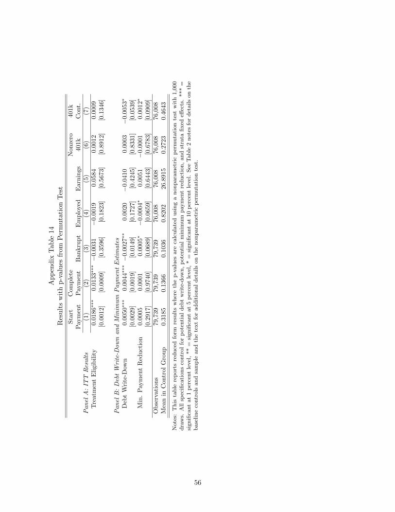
Ap

pen

dix

Tab

le14

Res

ult

sw

ith

p-v

alu

esfr

omP

erm

uta

tion

Tes

t

Sta

rtC

om

ple

teN

on

zero

401k

Pay

men

tP

aym

ent

Ban

kru

pt

Em

plo

yed

Earn

ings

401k

Cont.

Pan

elA

:IT

TR

esu

lts

(1)

(2)

(3)

(4)

(5)

(6)

(7)

Tre

atm

ent

Eli

gib

ilit

y0.0

186∗

∗∗0.0

133∗∗

∗−

0.0031

−0.

0019

0.0584

0.0012

0.0009

[0.0

012]

[0.0

009]

[0.3

596]

[0.1

823]

[0.5

673]

[0.8

912]

[0.1

346]

Pan

elB

:D

ebt

Wri

te-D

ow

nan

dM

inim

um

Paym

ent

Est

imate

sD

ebt

Wri

te-D

own

0.0

050∗

∗∗0.0

044∗∗

∗−

0.0027∗

∗0.0

020

−0.

0410

0.0003

−0.0

053∗

[0.0

029]

[0.0

019]

[0.0

149]

[0.1

727]

[0.4

245]

[0.8

331]

[0.0

539]

Min

.P

aym

ent

Red

uct

ion

0.0005

0.0001

0.0005∗

−0.0

004∗

0.0051

−0.

0001

0.0012∗

[0.2

917]

[0.9

740]

[0.0

689]

[0.0

659]

[0.6

443]

[0.6

783]

[0.0

909]

Ob

serv

atio

ns

79,7

39

79,7

39

79,7

39

76,0

08

76,0

08

76,0

08

76,0

08

Mea

nin

Con

trol

Gro

up

0.3

185

0.1

366

0.1

036

0.8

202

26.8

915

0.2723

0.4

643

Note

s:T

his

table

rep

ort

sre

duce

dfo

rmre

sult

sw

her

eth

ep-v

alu

esare

calc

ula

ted

usi

ng

anonpara

met

ric

per

muta

tion

test

wit

h1,0

00

dra

ws.

All

spec

ifica

tions

contr

ol

for

pote

nti

al

deb

tw

rite

-dow

n,

pote

nti

al

min

imum

pay

men

tre

duct

ion,

and

stra

tafixed

effec

ts.

***

=si

gnifi

cant

at

1p

erce

nt

level

,**

=si

gnifi

cant

at

5p

erce

nt

level

,*

=si

gnifi

cant

at

10

per

cent

level

.See

Table

2note

sfo

rdet

ails

on

the

base

line

contr

ols

and

sam

ple

and

the

text

for

addit

ional

det

ails

on

the

nonpara

met

ric

per

muta

tion

test

.

56

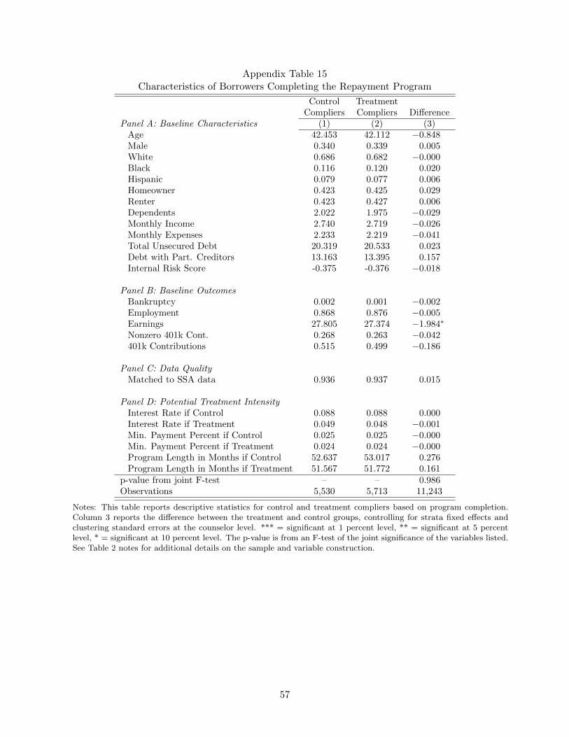
Appendix Table 15Characteristics of Borrowers Completing the Repayment Program

Control TreatmentCompliers Compliers Difference

Panel A: Baseline Characteristics (1) (2) (3)Age 42.453 42.112 −0.848Male 0.340 0.339 0.005White 0.686 0.682 −0.000Black 0.116 0.120 0.020Hispanic 0.079 0.077 0.006Homeowner 0.423 0.425 0.029Renter 0.423 0.427 0.006Dependents 2.022 1.975 −0.029Monthly Income 2.740 2.719 −0.026Monthly Expenses 2.233 2.219 −0.041Total Unsecured Debt 20.319 20.533 0.023Debt with Part. Creditors 13.163 13.395 0.157Internal Risk Score -0.375 -0.376 −0.018

Panel B: Baseline OutcomesBankruptcy 0.002 0.001 −0.002Employment 0.868 0.876 −0.005Earnings 27.805 27.374 −1.984∗

Nonzero 401k Cont. 0.268 0.263 −0.042401k Contributions 0.515 0.499 −0.186

Panel C: Data QualityMatched to SSA data 0.936 0.937 0.015

Panel D: Potential Treatment IntensityInterest Rate if Control 0.088 0.088 0.000Interest Rate if Treatment 0.049 0.048 −0.001Min. Payment Percent if Control 0.025 0.025 −0.000Min. Payment Percent if Treatment 0.024 0.024 −0.000Program Length in Months if Control 52.637 53.017 0.276Program Length in Months if Treatment 51.567 51.772 0.161

p-value from joint F-test – – 0.986Observations 5,530 5,713 11,243

Notes: This table reports descriptive statistics for control and treatment compliers based on program completion.Column 3 reports the difference between the treatment and control groups, controlling for strata fixed effects andclustering standard errors at the counselor level. *** = significant at 1 percent level, ** = significant at 5 percentlevel, * = significant at 10 percent level. The p-value is from an F-test of the joint significance of the variables listed.See Table 2 notes for additional details on the sample and variable construction.

57

Appendix Table 16Additional Characteristics of Borrowers Completing the Repayment Program

Control Treated x Treated x p-value onCompliers ∆ Rate ∆ Payment joint test

(1) (2) (3) (4)Age 42.4527 −0.4963 0.1077 0.5531

(13.7647) (0.4597) (0.1174)Male 0.3395 −0.0074 0.0022 0.8772

(0.4736) (0.0160) (0.0045)White 0.6864 −0.0025 −0.0008 0.8698

(0.4640) (0.0145) (0.0043)Black 0.1161 0.0062 0.0005 0.3784

(0.3204) (0.0111) (0.0030)Hispanic 0.0794 0.0034 −0.0001 0.9205

(0.2704) (0.0122) (0.0030)Homeowner 0.4231 −0.0069 0.0031 0.7479

(0.4941) (0.0141) (0.0041)Renter 0.4228 0.0083 −0.0028 0.7803

(0.4940) (0.0132) (0.0041)Dependents 2.0215 −0.0073 0.0025 0.9738

(1.2949) (0.0425) (0.0108)Monthly Income 2.7403 −0.0257 0.0068 0.8811

(1.5393) (0.0543) (0.0144)Monthly Expenses 2.2329 −0.0238 0.0052 0.8838

(1.3220) (0.0480) (0.0131)Total Unsecured Debt 20.3186 −0.3085 0.0555 0.8191

(16.6758) (0.4883) (0.1246)Debt with Part. Creditors 13.1625 −0.3097 0.0578 0.7011

(13.3711) (0.3676) (0.0966)Internal Risk Score -0.3754 0.0087 −0.0048 0.6907

(0.8569) (0.0299) (0.0071)Bankruptcy 0.0024 −0.0001 0.0000 0.9863

(0.0484) (0.0012) (0.0002)Employment 0.8680 0.0051 −0.0015 0.8880

(0.3385) (0.0109) (0.0033)Earnings 27.8054 −0.7406 0.0652 0.4203

(22.6910) (0.7042) (0.2127)Nonzero 401k Cont. 0.2676 −0.0062 −0.0006 0.6914

(0.4428) (0.0140) (0.0038)401k Contributions 0.5149 −0.0405 0.0019 0.4111

(1.1580) (0.0415) (0.0105)Matched to SSA data 0.9358 −0.0014 0.0005 0.9662

(0.2451) (0.0081) (0.0021)Observations 5,530 11,243

Notes: This table reports additional tests of the difference between control and treatment compliers based on programcompletion. We report coefficients on the interaction of treatment and potential treatment intensity. All regressionscontrol for potential treatment intensity and strata fixed effects, and cluster standard errors at the counselor level.Column 4 reports the p-value from an F-test that all interactions are jointly equal to zero. *** = significant at 1percent level, ** = significant at 5 percent level, * = significant at 10 percent level. See Table 2 notes for additionaldetails on the sample and variable construction.

58

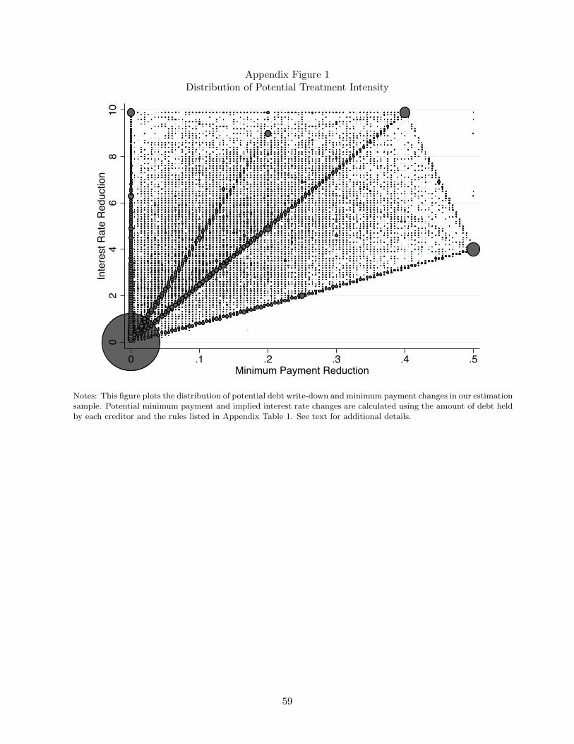
Appendix Figure 1Distribution of Potential Treatment Intensity

02

46

810

Inte

rest

Rat

e R

educ

tion

0 .1 .2 .3 .4 .5Minimum Payment Reduction

Notes: This figure plots the distribution of potential debt write-down and minimum payment changes in our estimationsample. Potential minimum payment and implied interest rate changes are calculated using the amount of debt heldby each creditor and the rules listed in Appendix Table 1. See text for additional details.

59

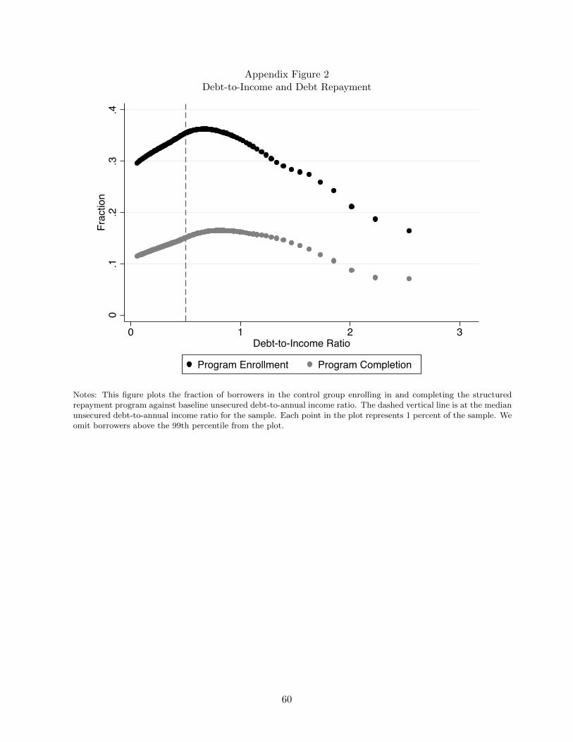
Appendix Figure 2Debt-to-Income and Debt Repayment

0.1

.2.3

.4Fr

actio

n

0 1 2 3Debt-to-Income Ratio

Program Enrollment Program Completion

Notes: This figure plots the fraction of borrowers in the control group enrolling in and completing the structuredrepayment program against baseline unsecured debt-to-annual income ratio. The dashed vertical line is at the medianunsecured debt-to-annual income ratio for the sample. Each point in the plot represents 1 percent of the sample. Weomit borrowers above the 99th percentile from the plot.

60

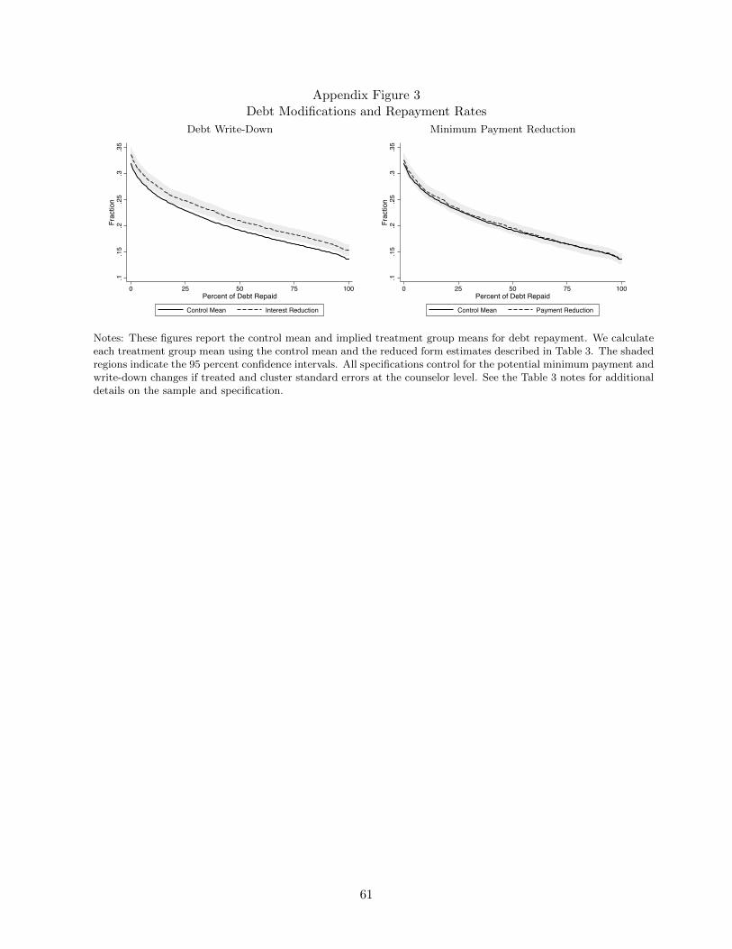
Appendix Figure 3Debt Modifications and Repayment Rates

Debt Write-Down Minimum Payment Reduction.1

.15

.2.2

5.3

.35

Frac

tion

0 25 50 75 100Percent of Debt Repaid

Control Mean Interest Reduction

.1.1

5.2

.25

.3.3

5Fr

actio

n

0 25 50 75 100Percent of Debt Repaid

Control Mean Payment Reduction

Notes: These figures report the control mean and implied treatment group means for debt repayment. We calculateeach treatment group mean using the control mean and the reduced form estimates described in Table 3. The shadedregions indicate the 95 percent confidence intervals. All specifications control for the potential minimum payment andwrite-down changes if treated and cluster standard errors at the counselor level. See the Table 3 notes for additionaldetails on the sample and specification.

61

Appendix A: Model Details

A. Additional Details from the Model Setup

Let qt ∈ {0, 1} be a binary variable where qt = 1 denotes default in period t, and qt = 0 repayment

in t. The net cash flow v (t, q) associated with the default decision q in period t is:

v (t, 1) = x

v (t, 0) = yt − dt

Then, the continuation value V (t, q) of making decision q subject to the liquidity constraint v for

any time period 0 ≤ t < P is given by the present discounted value of the contemporaneous period

cash flow of decision q and the future value of expected future cash flows associated with q:

V (t, q) ≡ v (t, q) + Et

[max{qk}

∞∑k=t+1

βk−tv (k, qk)

](5)

s.t.qt ∈ {qt−1, 1}qt = 1 if yt − dt > v ∀t ≤ P

Letting Γ (q, t) denote the set of values q′

which satisfy constraints for qt+1 given qt = q, we can

rewrite Equation (5) as:

V (t, q) ≡ v (t, q) + βE

[max

q′∈Γ(q,t)

{V(t+ 1, q

′)}]

(6)

where v (t, q) is the individual’s contemporaneous period cash flow in period t, and

βE[maxq′∈Γ(q,t)

{V(t+ 1, q

′)}]

is the individual’s future value of expected future cash flows as-

sociated with default decision q in t.

The above setup implies that the value of default V d ≡ V (t, 1) simplifies to the discounted

value of receiving x in both the current period and all future periods:

V d =x

1− β(7)

as individuals discount the future with a common (across-time) subjective discount rate β.

Conversely, the value of repayment V r (t, y) ≡ V (t, 0; y) for periods 0 ≤ t < P consists of the

contemporaneous value of repayment y − d and the option value of being able to either repay or

default in future periods β[∫∞

v+d max{V r(t+ 1, y

′), V d

}dF(y′)

+ F (v + d)V d]:

V r (t, y) = y − d+ β

[∫ ∞v+d

max{V r(t+ 1, y

′), V d

}dF(y′)

+ F (v + d)V d

](8)

Note that the contemporaneous value of repayment vr (y) ≡ y − d depends on both income y and

62

the constant debt payment d, while the option value of being able to either repay or default in

future periods β[∫∞

v+d max{V r(t+ 1, y

′), V d

}dF(y′)

+ F (v + d)V d]

depends on the expected

value of repayment relative to default value in period t+ 1. This expected value of repayment also

explicitly includes the expected possibility of involuntary default in future periods. We let this

future value, or “option value,” of repayment be denoted by Qr (t).

Now, note that in period t = P , repayment implies solvency in the next period, implying that

the option value of repayment Qr (P ) is:

Qr (P ) = βE

[ ∞∑k=P+1

yk

]

E [Qr (P )] =βµ

1− β

further implying that the repayment value in period t = P is:

V r (P, y) = y − d+Qr (P )

= y − d+ βµ

1− β(9)

The model is characterized by the value of repayment in period t = P given by Equation (9)

above, and the Bellman equation that gives the repayment continuation value V r (t, y) in periods

0 ≤ t < P . We form this Bellman equation by combining Equations (7) and (8):

V r (t, y) = y − d + β[∫

max{V r(t+ 1, y

′), x

1−β

}dF(y′)]

(10)

Equation (10) shows that while contemporaneous net income vr (y) = y − d is unaffected by t for

t < P , the option value of continuing repayment Qr (t) is weakly increasing in t for 0 ≤ t < P . This

is because the absence of payments or liquidity risk for solvent individuals in periods t > P means

the option value of repayment increases as individuals approach the end of the repayment period.

As a result, the total value of repayment V r (t, y) is also weakly increasing in t for 0 ≤ t < P .

B. Solving for Individuals’ Default Decision

The model implies that default decisions are driven by two separate forces: (1) involuntary default

that occurs among individuals who are liquidity constrained, and (2) the strategic response to low

income draws among individuals who are not liquidity constrained.

To see this, first recall that the liquidity constraint implies automatic default for individuals

with y ≤ v + d. Next, note that default occurs for individuals with y > v + d if and only if

V r (t, y) < V d, where the value of repayment V r (t, y) is strictly increasing in y. This implies that

optimal default behavior for a liquid individual can be characterized by a path of cutoff values φ∗t ,

defined by:

V r (t, φ∗t ) = V d

63

where a individual defaults if yt < φ∗t . Taken together, these two facts imply that general default

behavior can be characterized by φt:

q (t, y) =

1 if y ≤ φt0 if y > φt

(11)

φt = max (φ∗t , v + d) (12)

To solve for the path of φ∗ in periods 0 ≤ t ≤ P , we use the decision rule given by Equation

(11) to write the individuals’ Bellman equation (10) as:

V r (t, y) = y − d+ β

(∫ ∞φt+1

V r(t+ 1, y

′)dF(y′)

+ F (φt+1)V d

)(13)

Next, we use the fact that individuals are indifferent between repayment and default when the

income draw is equal to the cutoff (i.e., V r (t, φ∗t ) = V d) to show that:

V r (t, φ∗t ) =x

1− β(14)

and

vr (t, φ∗t ) +Qr (t) =x

1− βQr (t) =

x

1− β− φ∗t + d (15)

where Qr (t) again denotes the option value of expected future cash flows under repayment. We

can then substitute Equations (14) and (15) into the Bellman equation given by (13) to solve for

the path of default cutoffs φ∗t for liquid individuals in periods 0 ≤ t ≤ P :

V r (t, φ∗t ) = φ∗t − d+ β

[∫ ∞φt+1

V r(t+ 1, y

′)dF(y′)

+ F (φt+1)V d

]x

1− β= φ∗t − d+ β

[∫ ∞φt+1

[y′ − d+Qr (t+ 1)

]dF(y′)

+ F (φt+1)

(x

1− β

)]x

1− β= φ∗t − d+ β

[∫ ∞φt+1

[y′ − d+

(x

1− β− φ∗t+1 + d

)]dF(y′)

+ F (φt+1)

(x

1− β

)]

φ∗t =x

1− β+ d− β

[∫ ∞φt+1

(y′+

x

1− β− φ∗t+1

)dF(y′)

+ F (φt+1)

(x

1− β

)](16)

Following the discussion in the main text, Equation (16) implies that the optimal default cutoffs

φ∗t are strictly decreasing over time, reflecting the decreased incentive to default as individuals

remaining loan balances shrink.

Equation (16) and the fact that the liquidity constraint implies automatic default for individuals

64

with y ≤ v + d imply that the general decision rule φt that applies to both liquid and illiquid

individuals is:

φt = d+ max

{x

1− β− β

[∫ ∞φt+1

(y′+

x

1− β− φ∗t+1

)dF(y′)

+ F (φt+1)

(x

1− β

)], v

}(17)

Finally, we can fully characterize the path {φt} by using Equations (9) and (14) to find φP , the

cutoff in period t = P :

V r (P, φ∗P ) = V d

φ∗P − d+βµ

1− β=

x

1− β

φ∗P = d+x− βµ1− β

φP = d+ max

{x− βµ1− β

, v

}(18)

Default cutoffs φt for 0 ≤ t < P can be found via backward recursion using the difference equation

given by Equation (17) and the explicit solution for φP given by Equation (18).

C. Default Likelihood and Repayment

To examine the impact of the experiment on repayment rates through two different channels,

we must show how the default behavior described by Equation (17) affects the probability of

individuals’ remaining in repayment through period t. To do this, we first define an expression for

risk of default among repaying individuals at period t:

λ (t) ≡

F (φt) if t ≤ P

0 if t > P

where we note that the hazard rate λ (t) is weakly decreasing as individuals approach the end of

repayment. This result is due to the path of optimal default cutoffs φt strictly decreasing for all

0 ≤ t < P . Also note that the hazard rate λ (t) is strictly decreasing as individuals approach the

end of repayment if F (·) is assumed to increase strictly for all 0 ≤ t < P .

We then decompose the hazard rate λ (t) into strategic and non-strategic default risks:

λ (t) ≡ ρ (t) + γ (t) (19)

65

where

γ (t) ≡

F (v + d) if t ≤ P

0 if t > P(20)

ρ (t) ≡

∫ φtv+d dF (y) if t ≤ P

0 if t > P(21)

To map the hazard rates from each channel into the repayment rates observed in the experiment,

we first define the probability of remaining in repayment by period θ (t) as:

θ (t) ≡t∏

k=0

[1− λ (k)] (22)

using the fact that λ (t) is the conditional likelihood of exiting repayment at t. Letting the prob-

ability of avoiding default throughout the repayment period be Θ ≡ θP , we then have that the

probability of avoiding default through the entire repayment period Θ is:

Θ =

P∏t=0

[1− λ (t)] (23)

Using this framework, we can now investigate the implications of the experiment on the default

likelihood λ (t; ξ) as a function of the period t and repayment plan parameter ξ (e.g. repayment

period P , minimum payment d, etc.). To see this, note that Equation (19) implies:

λ (t; ξ) = ρ (t; ξ) + γ (t; ξ)

Strategic Risk Non-Strategic Risk

which gives us the model’s predicted repayment probability Θ:

Θ (ξ) =

t∏t=0

[1− λ (t; ξ)]

=

t∏t=0

[1− ρ (t; ξ)− γ (t; ξ)] (24)

where we have the familiar result that repayment rates are driven by two factors: (1) involuntary

default that occurs among individuals who are liquidity constrained, and (2) the strategic response

to low income draws among individuals who are not liquidity constrained.

66

D. Proofs of Model Predictions

D.1 Proof of Debt Write-Down Prediction

In this section, we expand on the discussion of the debt write-down effect from the main text before

providing a formal proof of the debt write-down prediction.

Preliminaries: The write-down treatment shortens the repayment period P to PWD < PC while

keeping the monthly payments d the same dWD = dC . Our model predicts that the write-down

treatment increases debt repayment through two complimentary effects: (1) a decrease in treated

individuals’ incentive to strategically default while both treatment and control individuals are

enrolled in the repayment program, and (2) a decrease in treated individuals’ exposure to default

risk while control individuals are still enrolled in the repayment program and treatment individuals

are not.

To formally establish these predictions, we first consider how the treatment reduces the “strate-

gic risk” of default in periods 0 ≤ t ≤ PWD:

∆ρ ≈ ∂ρ (t;P )

∂P∆P < 0 (25)

The direction of the strategic channel is weakly positive because a shorter repayment period in-

creases individuals’ strategic incentive to stay in repayment, thereby reducing strategic default

probability among treated individuals. This is because the lifetime of debt has been shortened

PC − PWD periods, leading treated individuals to place more value on repayment in each time

period t. Formally, it can be shown that:

∂φ∗ (t;P )

∂P=

∂E [V r (t, y)]

∂t∂ρ (t;P )

∂P= −∂ρ (t)

∂t

Implying that the shorter repayment period decreases optimal default cutoffs at exactly the rate

that expected continuation value increases over time. Intuitively, shortening repayment lengths

brings individuals closer to the point of solvency t = P , making it possible for these individuals

to accept lower net income in t in anticipation greater income in future time periods. As a result,

there is an increase in the mean continuation value E [V r (t, y)] for all 0 ≤ t < PWD, resulting in a

lower strategic cutoff φ∗t .

Note that effects through the strategic risk channel in periods 0 ≤ t ≤ PWD are tempered by the

presence of liquidity constraints, as changes in strategic default behavior are only realized for liquid

individuals (i.e. yt > v +d). In other words, the change in default cutoffs ∆φ (t) = φWD (t)−φC (t)

can only be so large in magnitude because φWD (t) and φC (t) are bounded below by v + d.

Next, we consider the non-strategic default likelihood in periods 0 ≤ t ≤ PWD:

∆γ ≈ ∂γ (t;P )

∂P∆P = 0 (26)

67

In contrast to this strategic effect in periods 0 ≤ t ≤ PWD, the non-strategic default likelihood in

periods 0 ≤ t ≤ PWD is exactly zero. This is because the liquidity constraint v + d is the same

for both the treatment and control groups in periods t ≤ PWD, meaning that treated individuals

are no more or less liquid. There is therefore zero effect through the non-strategic channel in these

time periods.

Finally, we consider both the strategic and non-strategic default probabilities in periods PWD <

t ≤ PC . By assumption, “repayment” in these periods is automatic for treated individuals that

have not defaulted by PWD. In contrast, control individuals are still exposed to both strategic and

non-strategic default risk. Differences in default rates are therefore given by:

∆λ (t) = 0− λC (t)

= −ρC (t)− γC (t)

where we have the result that default risk has decreased mechanically through both strategic and

non-strategic channels. Again, this is because control individuals still face the possibility of both

voluntary or involuntary default, while both forms of default risk have been eliminated for treated

individuals.

Proof of Debt Write-Down Prediction: Given the above insights concerning default likelihood

throughout the experiment, we can now predict the effect of lower debt write-downs on the change

in repayment rates ∆θ. First, consider θ(PWD

), the treatment effect at t = PWD, which is given

by:

∆θ(PWD

)≡ θWD

(PWD

)− θC

(PWD

)=

PWD∏t=0

[1− λWD (t)

]−PWD∏t=0

[1− λC (t)

]=

PWD∏t=0

[1− γ − ρWD (t)

]−PWD∏t=0

[1− γ − ρC (t)

]where γ = F (v + d) is non-strategic risk and ρWD (t), ρC (t) is period-t strategic default risk for

treatment and control. Importantly, since non-strategic risk γ is identical for both treatment and

control individuals, the treatment effect at ∆θ(PWD

)is driven entirely by differences in strategic

default behavior φ∗ (t).

68

That total treatment effect ∆Θ = ∆θ(PC)

is given by:

∆Θ = ΘWD −ΘC

=PC∏t=0

[1− λWD (t)

]−

PC∏t=0

[1− λC (t)

]=

PWD∏t=0

[1− λWD (t)

]−PWD∏t=0

[1− λC (t)

] PC∏t=PWD+1

[1− λC (t)

]

= θWD(PWD

)− θC

(PC) PC∏

t=PWD+1

[1− λWD (t)

]Since

∏PC

t=PWD+1

[1− λC (t)

]< 1, the total treatment effect is larger than the period PWD treat-

ment effect, i.e. ∆Θ ≥ ∆θ(PWD

).

D.2 Proof of Minimum Payment Prediction

Following the proof of the debt write-down prediction, we first expand on the discussion of the

minimum payment effect from the main text before providing a formal proof of the minimum

payment prediction.

Preliminaries: The minimum payment treatment reduces the required minimum payment by

lengthening the repayment period. In the context of our model, a lower minimum payment can

therefore be thought of as lengthening the repayment period P to PMP > PC while keeping the

total debt burden the same∑PC

t=0 dt =∑PMP

t=0 dt. Our model predicts an ambiguous impact of

the minimum payment treatment on repayment rates due to three opposing effects: (1) a decrease

in treated individuals’ non-strategic or liquidity-based default while both treatment and control

individuals are enrolled in the repayment program, (2) an ambiguous change in treated individu-

als’ incentive to strategically default while both treatment and control individuals are enrolled in

the repayment program, and (3) an increase in treated individuals’ exposure to default risk while

treated individuals are still enrolled in the repayment program and control individuals are not.

To formally establish these predictions, we first alter the model to make monthly payment d

endogenous. Specifically, we let D denote the individuals debt balance at t = 0 and treat repayment

amounts d as function of their total debt D and repayment period length P :

d = d (P,D) =D

P

Modifying Equation (10), we now have:

V r (t) = y − d (P,D) + βE[max

{V r(t+ 1, y

′), V d

(y′)}]

To consider the effects of an increase in P , we must investigate how strategic and non-strategic

69

risk respond to both a greater repayment length and lower minimum payments. We first restrict

our attention to periods in which neither group has reached solvency (0 ≤ t ≤ PC). Consider

treatment’s effect on strategic default risk ρ (t), holding liquidity constraints fixed. We have:

∆ρ ≈ ∂ρ(t;P,d)∂P ∆P + ∂ρ(t;P,d)

∂d∂d∂P ∆P

Solvency Effect (+) Payment Effect (-)R 0 (27)

The direction of the strategic channel is ambiguous because two opposing forces influence individ-

uals’ considerations of whether or not default is optimal. First, extending the number of periods in

which individuals make payments will, all else equal, increase strategic risk (∂ρ(P,d)∂P ∆P > 0). This

is the same as the effect from the debt write-down treatment (25), only in the opposite direction.

Thus, as the end of repayment P moves farther away, the option value of repayment is lower because

treated individuals anticipate a more difficult road to solvency. On the other hand, the decrease

in minimum payment size will decrease default risk (∂ρ(P,d)∂d

∂d∂P ∆P < 0), as lower payments mean

higher cash flows both presently and in expectation. The net direction of changes in strategic risk

depends on the relative magnitude of “solvency” and “payment” effects, which vary according to

the period. In t = 0, the payment effect must dominate and strategic concerns must have a net

negative effect on default likelihood. This is due to the fact that the minimum payment treatment

only lowers the minimum payments individuals have to pay, repayment under the terms of control

individuals (i.e. higher minimum payments and shorter repayment length) is still in each treated

individual’s choice set. Therefore, repayment in period t = 0 must be at least as attractive as

it would have been under control conditions. However, as each period passes, control individuals

have paid an increasingly larger portion of their debt burden D relative to treated individuals. As

t approaches the end of control repayment period PC , control individuals have already repaid all

but a small portion of their debt(DPC

), whereas treated individuals have a remaining loan balance

of ∆P ∗ DPMP , and thus have less incentive to avoid default.

Now consider treatment’s effect on non-strategic default risk γ (t) in periods 0 ≤ t ≤ PC . We

have:

∆γ ≈ ∂γ

∂d

∂d

∂P∆P < 0 (28)

In contrast to the strategic channel, the non-strategic channel has an unambiguously negative effect

on default risk. Liquidity constraints are less likely to bind under treatment (∂γ∂d∂d∂P ∆P < 0) because

payments are lower and net income is higher. So, holding her strategy fixed, a treated individual

is less likely to be forced into involuntary default in periods t ≤ PC because repayment has been

made less onerous in these periods. Note that this only affects total default probability λ (t) if some

“illiquid” control individuals would optimally repay (i.e. φ∗ (t) < v +dC and ρ (t) = 0). Otherwise,

differences in liquidity only occur among individuals who would default anyway.

Finally, we consider periods PC < t ≤ PMP . Just as it was for treated individuals under the

debt write-down treatment, under minimum payment treatment debt has been completely forgiven

70

for control individuals in these periods. Using Equation (24), we have:

∆λ (t) = λMP (t)− 0

= ρMP (t) + γMP (t)

The difference in default probability between treatment and control for any period PC < t ≤ PMP

is simply the sum of strategic and liquidity risk components contributing to default risk for treated

individuals who are still in repayment.

Proof of Minimum Payment Prediction: We can now use these insights to predict treatment effects

∆θ. First, consider θ(PC), the treatment effect at t = PC , given by:

∆θ(PC)≡ θMP

(PC)− θC

(PC)

=PC∏t=0

[1− γMP (t)− ρMP (t)

]−

PC∏t=0

[1− γC (t)− ρC (t)

]where γMP (t), γC (t) is non-strategic and ρMP (t), ρC (t) is strategic default risk in period t for

treatment and control groups. As we established above, lower payments implies lower non-strategic

risk for treated individuals (γMP (t) − γC (t) < 0), but the difference in strategic default risk

ρMP (t)−ρC (t) is ambiguous in both size and magnitude due to the countervailing forces associated

with making a lower payment for a longer time period. The lower minimum payment treatment

therefore has an ambiguous impact on repayment rates at PC .

The total treatment effect Θ = θ(PMP

)is given by:

∆Θ = ΘMP −ΘC

=PMP∏t=0

[1− λMP (t)

]−PMP∏t=0

[1− λC (t)

]=

PMP∏t=0

[1− λMP (t)

] PMP∏t=PC+1

[1− λMP (t)

]−

PC∏t=0

[1− λC (t)

]

= θMP(PWD

) PC∏t=PWD+1

[1− λMP (t)

]− θC (PC)

Since∏PMP

t=PC+1

[1− λMP (t)

]< 1, the total treatment effect is smaller than the period PC treat-

ment effect, i.e. ∆Θ ≤ ∆θ(PC).

71