dba 4: analyzing data - o'reilly mediaarchive.oreilly.com/oreillyschool/courses/dba4/dba...
TRANSCRIPT
DBA 4: Analyzing DataLesson 1: Int ro duct io n
Understanding the Learning Sandbox Environment
What is MDX?Your First MDX Query
Lesson 2: MDX Fro m t he Gro und UpThe Basics
What is a Cube?Basic MDX QueriesData Types
Lesson 3: T uples and Set sTuples and Sets
TuplesSets
Navigating the Cube
Lesson 4: Calculat ed MembersCalculated Members
Format Strings
Named Sets
Lesson 5: MDX Funct io ns, Part IUnion and Cross Jo in
Other Set Functions
Lesson 6 : MDX Funct io ns, Part IIFiltering Data
Functions for Hierarchies
Lesson 7: T raveling in T imeCommon Date Questions
Year to DateComparing Sales from Month to MonthPrior QuarterParallel Periods
Lesson 8 : T o p QueriesTop
Generate
Lesson 9 : Predict ing t he Fut ureHow to Predict the Future
Predicting the Future with MDX
Lesson 10: Mo ndrian SchemasWriting a Basic Schema
The Structure o f a SchemaXML Documents

Shared DimensionsCube
Lesson 11: Advanced SchemasCalculated Members
Virtual Cubes
Lesson 12: Final Pro jectYour Final Pro ject
SchemaQueries
Copyright © 1998-2014 O'Reilly Media, Inc.
This work is licensed under a Creative Commons Attribution-ShareAlike 3.0 Unported License.See http://creativecommons.org/licenses/by-sa/3.0/legalcode for more information.

Introduction
Welcome to DBA 4, the final course in the O'Reilly DBA Series!
Course ObjectivesWhen you complete this course, you will be able to :
demonstrate the basics o f MDX, the query language o f data warehouses.analyze and extrapo late business models through data modeling.write a schema for Mondrian - the XML document that bridges the relational and multidimensional worlds.
In this course you'll learn how to take your MySQL knowledge to the next level. You'll learn how to take their relational datawarehouse to the next level using Mondrian and JPivot, two too ls fo r Multidimensional data analysis. We'll assume you haveworked through the first three courses in the series, are familiar with MySQL, and understand data warehousing concepts. Feelfree to revisit the previous courses at any time to refresh your memory about any concepts we learned earlier.
You'll learn by do ing pro jects in your own Unix and MySQL environments, and then handing them in for instructor feedback.These pro jects, as well as the final pro ject, add to your portfo lio and will contribute to certificate completion. Besides a browserand internet connection, all so ftware is provided online by the O'Reilly School o f Technology.
Learning with O'Reilly School of Technology CoursesAs with every O'Reilly School o f Technology course, we'll take a user-active approach to learning. This means that you(the user) will be active! You'll learn by do ing, building live programs, testing them and experimenting with them—hands-on!
To learn a new skill o r techno logy, you have to experiment. The more you experiment, the more you learn. Our systemis designed to maximize experimentation and help you learn to learn a new skill.
We'll program as much as possible to be sure that the principles sink in and stay with you.
Each time we discuss a new concept, you'll put it into code and see what YOU can do with it. On occasion we'll evengive you code that doesn't work, so you can see common mistakes and how to recover from them. Making mistakesis actually another good way to learn.
Above all, we want to help you to learn to learn. We give you the too ls to take contro l o f your own learning experience.
When you complete an OST course, you know the subject matter, and you know how to expand your knowledge, soyou can handle changes like software and operating system updates.
Here are some tips for using O'Reilly School o f Technology courses effectively:
T ype t he co de. Resist the temptation to cut and paste the example code we give you. Typing the codeactually gives you a feel fo r the programming task. Then play around with the examples to find out what elseyou can make them do, and to check your understanding. It's highly unlikely you'll break anything byexperimentation. If you do break something, that's an indication to us that we need to improve our system!T ake yo ur t ime. Learning takes time. Rushing can have negative effects on your progress. Slow down andlet your brain absorb the new information thoroughly. Taking your time helps to maintain a relaxed, positiveapproach. It also gives you the chance to try new things and learn more than you o therwise would if youblew through all o f the coursework too quickly.Experiment . Wander from the path o ften and explore the possibilities. We can't anticipate all o f yourquestions and ideas, so it's up to you to experiment and create on your own. Your instructor will help if yougo completely o ff the rails.Accept guidance, but do n't depend o n it . Try to so lve problems on your own. Going frommisunderstanding to understanding is the best way to acquire a new skill. Part o f what you're learning isproblem so lving. Of course, you can always contact your instructor fo r hints when you need them.Use all available reso urces! In real- life problem-so lving, you aren't bound by false limitations; in OSTcourses, you are free to use any resources at your disposal to so lve problems you encounter: the Internet,reference books, and online help are all fair game.Have f un! Relax, keep practicing, and don't be afraid to make mistakes! Your instructor will keep you at ituntil you've mastered the skill. We want you to get that satisfied, "I'm so coo l! I did it!" feeling. And you'll havesome pro jects to show off when you're done.

Lesson FormatWe'll try out lo ts o f examples in each lesson. We'll have you write code, look at code, and edit existing code. The codewill be presented in boxes that will indicate what needs to be done to the code inside.
Whenever you see white boxes like the one below, you'll type the contents into the editor window to try the exampleyourself. The CODE TO TYPE bar on top o f the white box contains directions for you to fo llow:
CODE TO TYPE:
White boxes like this contain code for you to try out (type into a file to run).
If you have already written some of the code, new code for you to add looks like this. If we want you to remove existing code, the code to remove will look like this. We may also include instructive comments that you don't need to type.
We may run programs and do some other activities in a terminal session in the operating system or o ther command-line environment. These will be shown like this:
INTERACTIVE SESSION:
The plain black text that we present in these INTERACTIVE boxes is provided by the system (not for you to type). The commands we want you to type look like this.
Code and information presented in a gray OBSERVE box is fo r you to inspect and absorb. This information is o ftenco lor-coded, and fo llowed by text explaining the code in detail:
OBSERVE:
Gray "Observe" boxes like this contain information (usually code specifics) for you to observe.
The paragraph(s) that fo llow may provide addition details on inf o rmat io n that was highlighted in the Observe box.
We'll also set especially pertinent information apart in "Note" boxes:
Note Notes provide information that is useful, but not abso lutely necessary for performing the tasks at hand.
Tip Tips provide information that might help make the too ls easier fo r you to use, such as shortcut keys.
WARNING Warnings provide information that can help prevent program crashes and data loss.
Understanding the Learning Sandbox EnvironmentIn this course we'll be using the MDX, Unix, and XML modes in CodeRunner:
What is MDX?MDX is a query language originally developed by Microsoft fo r its Analysis Services component o f SQL Server.Analysis Services is Microsoft's OLAP (online analytical processing) server. Since its release in 1997, MDX has beenembraced by many o ther data warehouse vendors, including the open source OLAP server Mondrian. In this coursewe will use Mondrian, however the core concepts also apply to o ther OLAP servers such as Analysis Services.
At the end o f the DBA 3 course, we learned how to query the data warehouse using SQL. So why would we want tolearn a different way to query? Well, you may recall that there are several potential pitfalls we could encounter whenusing SQL. We discussed two o f them in DBA 3 -- Bad Jo ins and Inco rrect Filt ering. While no computer languagecan keep you from making any mistakes, MDX makes it much less likely that these problems will occur.
The syntax o f MDX makes answering common data warehouse questions such as, "In 2008, how did the east region'ssales compare to those of the west region?," less complicated. The same query would be lengthy and complex usingSQL.
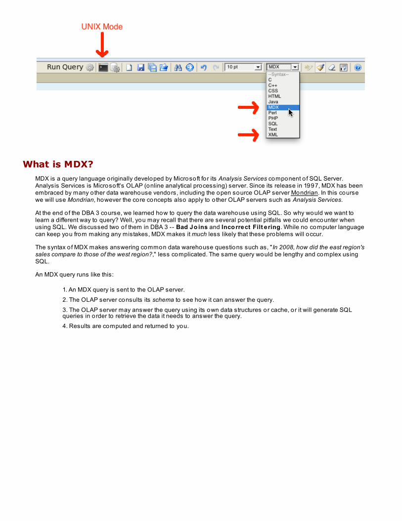
An MDX query runs like this:
1. An MDX query is sent to the OLAP server.2. The OLAP server consults its schema to see how it can answer the query.3. The OLAP server may answer the query using its own data structures or cache, or it will generate SQLqueries in order to retrieve the data it needs to answer the query.4. Results are computed and returned to you.
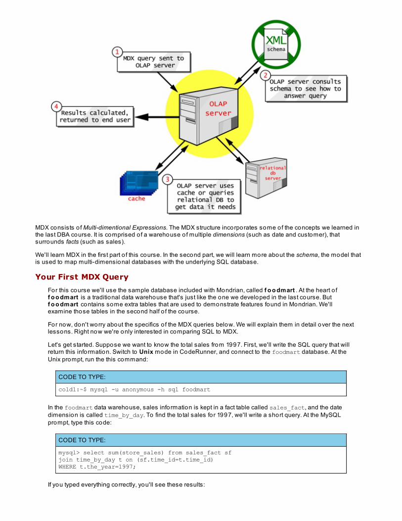
MDX consists o f Multi-dimentional Expressions. The MDX structure incorporates some of the concepts we learned inthe last DBA course. It is comprised o f a warehouse o f multiple dimensions (such as date and customer), thatsurrounds facts (such as sales).
We'll learn MDX in the first part o f this course. In the second part, we will learn more about the schema, the model thatis used to map multi-dimensional databases with the underlying SQL database.
Your First MDX Query
For this course we'll use the sample database included with Mondrian, called f o o dmart . At the heart o ff o o dmart is a traditional data warehouse that's just like the one we developed in the last course. Butf o o dmart contains some extra tables that are used to demonstrate features found in Mondrian. We'llexamine those tables in the second half o f the course.
For now, don't worry about the specifics o f the MDX queries below. We will explain them in detail over the nextlessons. Right now we're only interested in comparing SQL to MDX.
Let's get started. Suppose we want to know the to tal sales from 1997. First, we'll write the SQL query that willreturn this information. Switch to Unix mode in CodeRunner, and connect to the foodmart database. At theUnix prompt, run the this command:
CODE TO TYPE:
cold1:~$ mysql -u anonymous -h sql foodmart
In the foodmart data warehouse, sales information is kept in a fact table called sales_fact, and the datedimension is called time_by_day. To find the to tal sales for 1997, we'll write a short query. At the MySQLprompt, type this code:
CODE TO TYPE:
mysql> select sum(store_sales) from sales_fact sfjoin time_by_day t on (sf.time_id=t.time_id)WHERE t.the_year=1997;
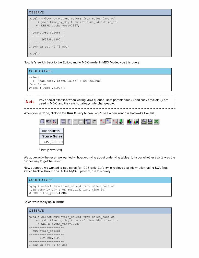
If you typed everything correctly, you'll see these results:
OBSERVE:
mysql> select sum(store_sales) from sales_fact sf -> join time_by_day t on (sf.time_id=t.time_id) -> WHERE t.the_year=1997;+------------------+| sum(store_sales) |+------------------+| 565238.1300 | +------------------+1 row in set (0.73 sec)
mysql>
Now let's switch back to the Editor, and to MDX mode. In MDX Mode, type this query:
CODE TO TYPE:
select { [Measures].[Store Sales] } ON COLUMNSfrom Saleswhere ([Time].[1997])
Note Pay special attention when writing MDX queries. Both parentheses () and curly brackets {} areused in MDX, and they are not always interchangeable.
When you're done, click on the Run Query button. You'll see a new window that looks like this:
We got exactly the result we wanted without worrying about underlying tables, jo ins, or whether SUM() was theproper way to get the result.
Now suppose we wanted to see sales for 1998 only. Let's try to retrieve that information using SQL first;switch back to Unix mode. At the MySQL prompt, run this query:
CODE TO TYPE:
mysql> select sum(store_sales) from sales_fact sfjoin time_by_day t on (sf.time_id=t.time_id)WHERE t.the_year=1998;
Sales were really up in 1998!
OBSERVE:
mysql> select sum(store_sales) from sales_fact sf -> join time_by_day t on (sf.time_id=t.time_id) -> WHERE t.the_year=1998;+------------------+| sum(store_sales) |+------------------+| 1199308.3100 | +------------------+1 row in set (1.54 sec)
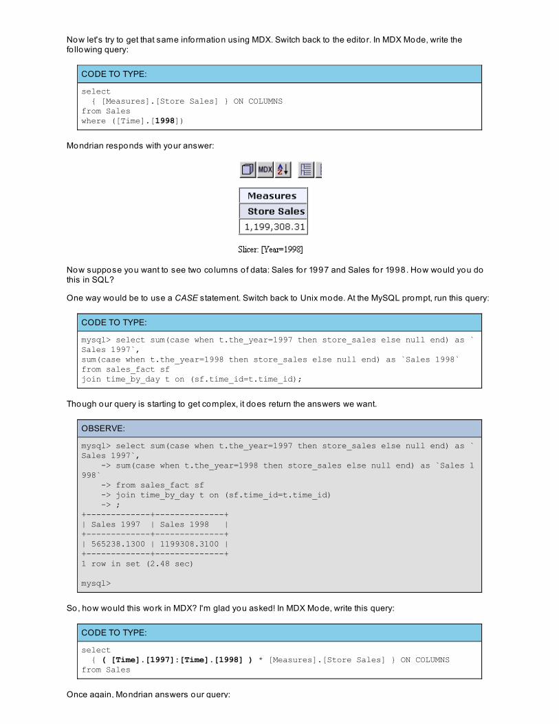
Now let's try to get that same information using MDX. Switch back to the editor. In MDX Mode, write thefo llowing query:
CODE TO TYPE:
select { [Measures].[Store Sales] } ON COLUMNSfrom Saleswhere ([Time].[1998])
Mondrian responds with your answer:
Now suppose you want to see two co lumns o f data: Sales for 1997 and Sales for 1998. How would you dothis in SQL?
One way would be to use a CASE statement. Switch back to Unix mode. At the MySQL prompt, run this query:
CODE TO TYPE:
mysql> select sum(case when t.the_year=1997 then store_sales else null end) as `Sales 1997`,sum(case when t.the_year=1998 then store_sales else null end) as `Sales 1998`from sales_fact sfjoin time_by_day t on (sf.time_id=t.time_id);
Though our query is starting to get complex, it does return the answers we want.
OBSERVE:
mysql> select sum(case when t.the_year=1997 then store_sales else null end) as `Sales 1997`, -> sum(case when t.the_year=1998 then store_sales else null end) as `Sales 1998` -> from sales_fact sf -> join time_by_day t on (sf.time_id=t.time_id) -> ;+-------------+--------------+| Sales 1997 | Sales 1998 |+-------------+--------------+| 565238.1300 | 1199308.3100 | +-------------+--------------+1 row in set (2.48 sec)
mysql>
So, how would this work in MDX? I'm glad you asked! In MDX Mode, write this query:
CODE TO TYPE:
select { ( [Time].[1997]:[Time].[1998] ) * [Measures].[Store Sales] } ON COLUMNSfrom Sales
Once again, Mondrian answers our query:
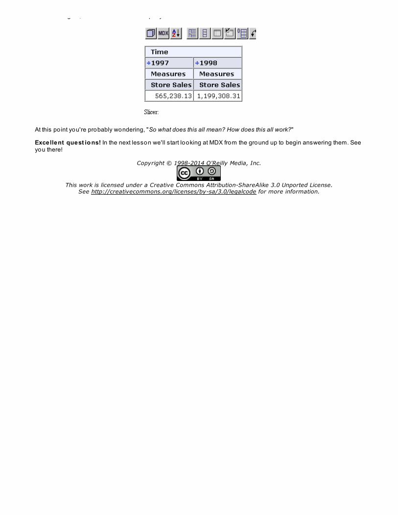
Once again, Mondrian answers our query:
At this po int you're probably wondering, "So what does this all mean? How does this all work?"
Excellent quest io ns! In the next lesson we'll start looking at MDX from the ground up to begin answering them. Seeyou there!
Copyright © 1998-2014 O'Reilly Media, Inc.
This work is licensed under a Creative Commons Attribution-ShareAlike 3.0 Unported License.See http://creativecommons.org/licenses/by-sa/3.0/legalcode for more information.
MDX From the Ground Up
The BasicsWelcome back!
In the last lesson we saw our first MDX queries. In this lesson, we'll discuss what makes MDX unique and compare itto SQL.
Note In MDX the term measure is commonly used instead o f the term fact. In this course we will use the termmeasure instead o f fact. For our purposes, these terms are synonymous with one another.
What is a Cube?
In the DBA 3 course, we learned how to organize our measures and dimensions to create a data warehouse,in order to answer questions like, "How much profit did we have on alcoholic beverages last month?" Werewrote that question in a slightly different fo rm to extract the f act s and dimensio ns: "How much profit didwe have by product and by month?"
Note In the last course we learned that data warehouses usually have a dat e dimension. Thewarehouse we are using in this course also has a dat e dimension, but it is called T ime .
We used a star schema to relate our measures and dimensions in our relational data warehouse. Thisstructure in the MDX world is known as a cube.
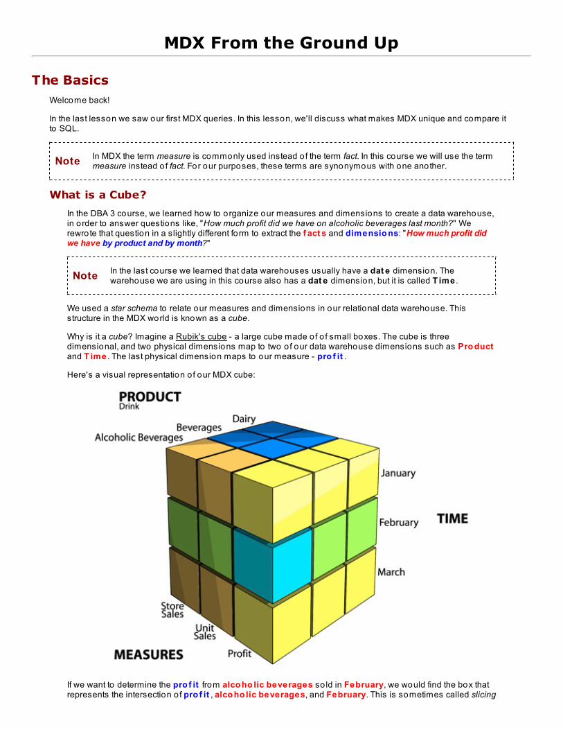
Why is it a cube? Imagine a Rubik's cube - a large cube made o f o f small boxes. The cube is threedimensional, and two physical dimensions map to two o f our data warehouse dimensions such as Pro ductand T ime . The last physical dimension maps to our measure - pro f it .
Here's a visual representation o f our MDX cube:
If we want to determine the pro f it from alco ho lic beverages so ld in February, we would find the box thatrepresents the intersection o f pro f it , alco ho lic beverages, and February. This is sometimes called slicing
or dicing the cube - imagine cutting open the Rubik's cube to retrieve the single box you are interested inexamining.
In the MDX world, dimensions and measures are not so different. In fact, the co llection o f measures comprisea special dimension that's called Measures.
Switch the editor to MDX mode and write this query:
CODE TO TYPE:
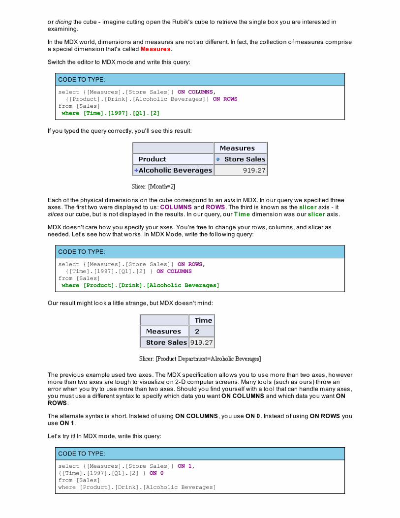
select {[Measures].[Store Sales]} ON COLUMNS, {[Product].[Drink].[Alcoholic Beverages]} ON ROWSfrom [Sales] where [Time].[1997].[Q1].[2]
If you typed the query correctly, you'll see this result:
Each o f the physical dimensions on the cube correspond to an axis in MDX. In our query we specified threeaxes. The first two were displayed to us: COLUMNS and ROWS . The third is known as the slicer axis - itslices our cube, but is not displayed in the results. In our query, our T ime dimension was our slicer axis.
MDX doesn't care how you specify your axes. You're free to change your rows, co lumns, and slicer asneeded. Let's see how that works. In MDX Mode, write the fo llowing query:
CODE TO TYPE:
select {[Measures].[Store Sales]} ON ROWS, {[Time].[1997].[Q1].[2] } ON COLUMNSfrom [Sales] where [Product].[Drink].[Alcoholic Beverages]
Our result might look a little strange, but MDX doesn't mind:
The previous example used two axes. The MDX specification allows you to use more than two axes, howevermore than two axes are tough to visualize on 2-D computer screens. Many too ls (such as ours) throw anerror when you try to use more than two axes. Should you find yourself with a too l that can handle many axes,you must use a different syntax to specify which data you want ON COLUMNS and which data you want ONROWS .
The alternate syntax is short. Instead o f using ON COLUMNS , you use ON 0 . Instead o f using ON ROWS youuse ON 1.
Let's try it! In MDX mode, write this query:
CODE TO TYPE:
select {[Measures].[Store Sales]} ON 1,{[Time].[1997].[Q1].[2] } ON 0from [Sales]where [Product].[Drink].[Alcoholic Beverages]
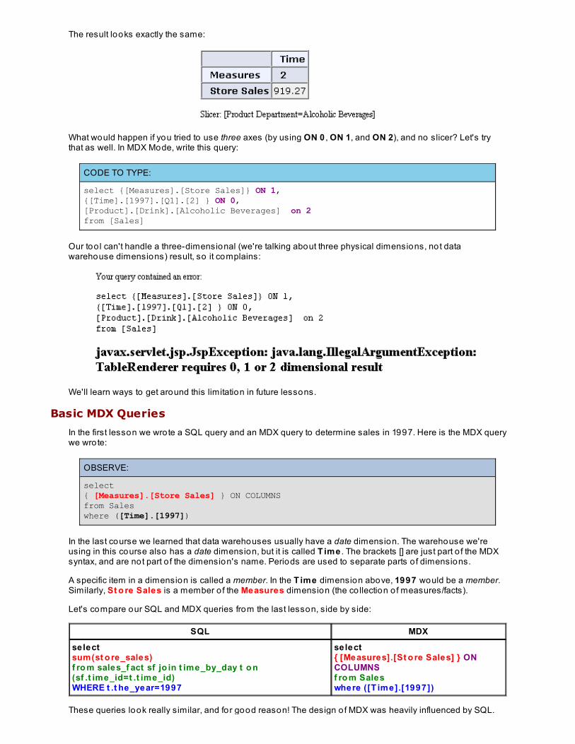
The result looks exactly the same:
What would happen if you tried to use three axes (by using ON 0 , ON 1, and ON 2), and no slicer? Let's trythat as well. In MDX Mode, write this query:
CODE TO TYPE:
select {[Measures].[Store Sales]} ON 1,{[Time].[1997].[Q1].[2] } ON 0,[Product].[Drink].[Alcoholic Beverages] on 2from [Sales]
Our too l can't handle a three-dimensional (we're talking about three physical dimensions, not datawarehouse dimensions) result, so it complains:
We'll learn ways to get around this limitation in future lessons.
Basic MDX Queries
In the first lesson we wrote a SQL query and an MDX query to determine sales in 1997. Here is the MDX querywe wrote:
OBSERVE:
select{ [Measures].[Store Sales] } ON COLUMNSfrom Saleswhere ([Time].[1997])
In the last course we learned that data warehouses usually have a date dimension. The warehouse we'reusing in this course also has a date dimension, but it is called T ime . The brackets [] are just part o f the MDXsyntax, and are not part o f the dimension's name. Periods are used to separate parts o f dimensions.
A specific item in a dimension is called a member. In the T ime dimension above, 1997 would be a member.Similarly, St o re Sales is a member o f the Measures dimension (the co llection o f measures/facts).
Let's compare our SQL and MDX queries from the last lesson, side by side:
SQL MDX
select sum(st o re_sales)f ro m sales_f act sf jo in t ime_by_day t o n(sf .t ime_id=t .t ime_id)WHERE t .t he_year=1997
select{ [Measures].[St o re Sales] } ONCOLUMNSf ro m Saleswhere ([T ime].[1997])
These queries look really similar, and for good reason! The design o f MDX was heavily influenced by SQL.
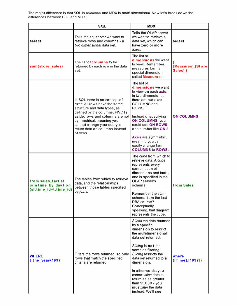
The major difference is that SQL is relational and MDX is multi-dimentional. Now let's break down thedifferences between SQL and MDX:
SQL MDX
selectTells the sql server we want toretrieve rows and co lumns - atwo dimensional data set.
Tells the OLAP serverwe want to retrieve adata set, which canhave zero or moreaxes.
select
sum(st o re_sales)The list o f co lumns to bereturned by each row in the dataset.
The list o fdimensio ns we wantto view. Remember,measures form aspecial dimensioncalled Measures.
{[Measures].[St o reSales] }
In SQL there is no concept o faxes. All rows have the samestructure and data types, asdefined by the co lumns. PIVOTsaside, rows and co lumns are notsymmetrical, meaning youcannot change your query toreturn data on co lumns insteadof rows.
The list o fdimensio ns we wantto view on each axis.In two dimensions,there are two axes:COLUMNS andROWS.
Instead o f specifyingON COLUMNS , youcould use ON ROWSor a number like ON 2.
Axes are symmetric,meaning you caneasily change fromCOLUMNS to ROWS .
ON COLUMNS
f ro m sales_f act sfjo in t ime_by_day t o n(sf .t ime_id=t .t ime_id)
The tables from which to retrievedata, and the relationshipsbetween those tables specifiedby joins.
The cube from which toretrieve data. A cuberepresents everycombination o fdimensions and facts,and is specified in theOLAP server'sschema.
Remember the starschema from the lastDBA course?Conceptuallyspeaking, that diagramrepresents the cube.
f ro m Sales
WHEREt .t he_year=1997
Filters the rows returned, so onlyrows that match the specifiedcriteria are returned.
Slices the data returnedby a specificdimension to restrictthe multidimensionaldata set returned.
Slicing is no t thesame as filtering.Slicing restricts thedata set returned to adimension.
In o ther words, youcannot slice data toreturn sales greaterthan $5,000 - youmust filter the datainstead. We'll see
where([T ime].[1997])
more on filtering later.
While MDX and SQL are similar in some respects, they are quite different in o thers.
Data Types
SQL databases have several different data types: integers, characters, decimals, and more. MDX has six datatypes:
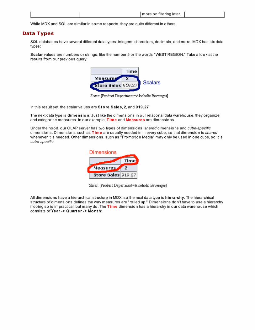
Scalar values are numbers or strings, like the number 5 or the words "WEST REGION." Take a look at theresults from our previous query:
In this result set, the scalar values are St o re Sales, 2, and 919.27
The next data type is dimensio n. Just like the dimensions in our relational data warehouse, they organizeand categorize measures. In our example, T ime and Measures are dimensions.
Under the hood, our OLAP server has two types o f dimensions: shared dimensions and cube-specificdimensions. Dimensions such as T ime are usually needed in in every cube, so that dimension is sharedwhenever it is needed. Other dimensions, such as "Promotion Media" may only be used in one cube, so it iscube-specific.
All dimensions have a hierarchical structure in MDX, so the next data type is hierarchy. The hierarchicalstructure o f dimensions defines the way measures are "ro lled up." Dimensions don't have to use a hierarchyif do ing so is impractical, but many do. The T ime dimension has a hierarchy in our data warehouse whichconsists o f Year -> Quart er -> Mo nt h:
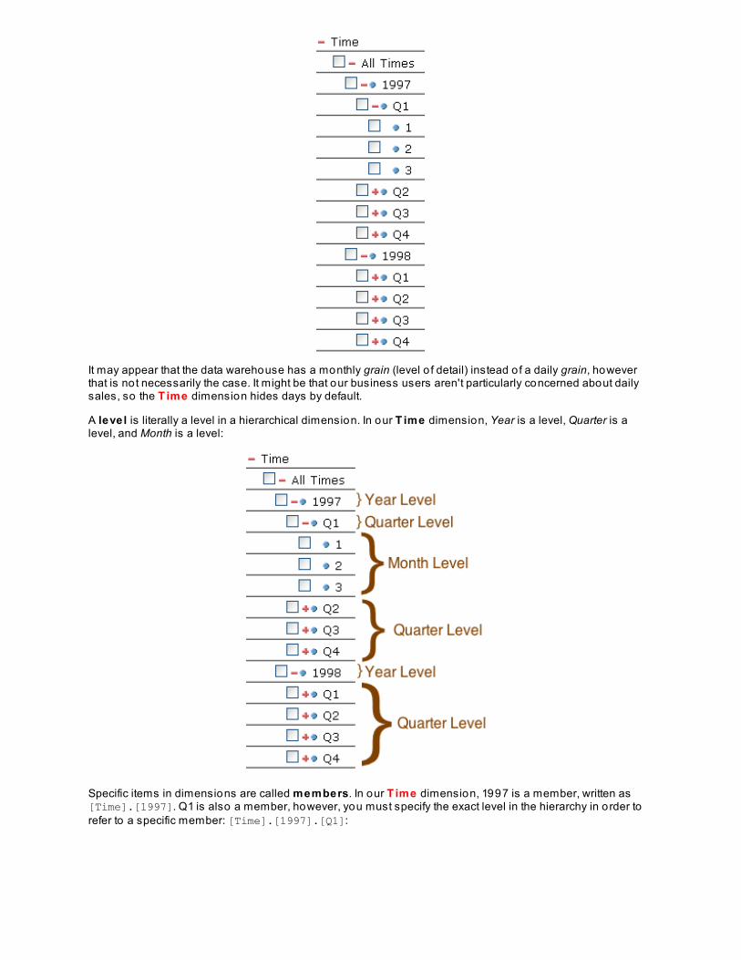
It may appear that the data warehouse has a monthly grain (level o f detail) instead o f a daily grain, howeverthat is not necessarily the case. It might be that our business users aren't particularly concerned about dailysales, so the T ime dimension hides days by default.
A level is literally a level in a hierarchical dimension. In our T ime dimension, Year is a level, Quarter is alevel, and Month is a level:
Specific items in dimensions are called members. In our T ime dimension, 1997 is a member, written as[Time].[1997]. Q1 is also a member, however, you must specify the exact level in the hierarchy in order torefer to a specific member: [Time].[1997].[Q1]:
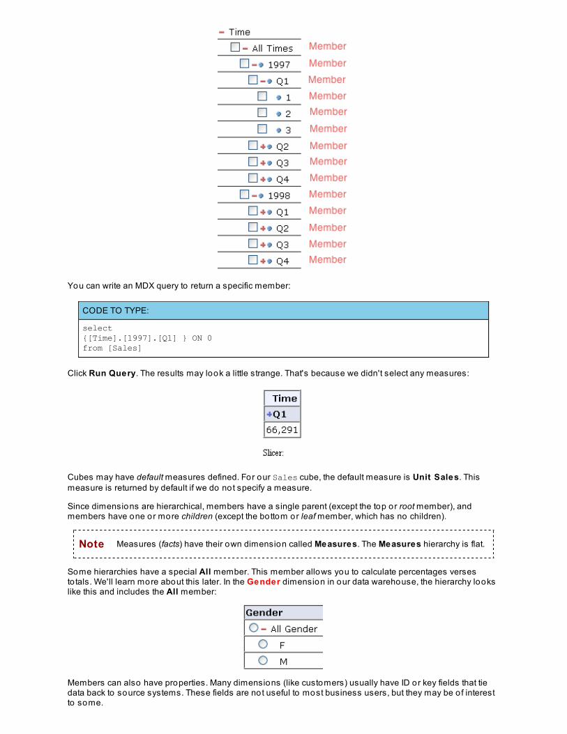
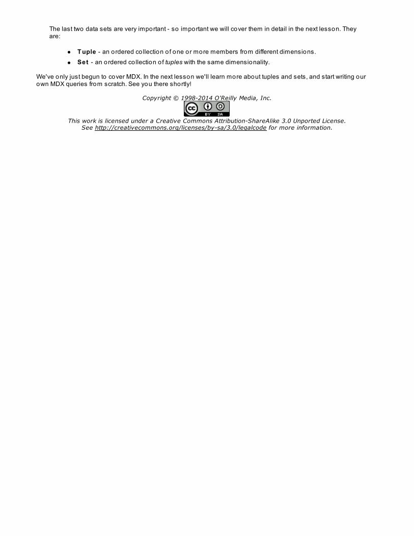
You can write an MDX query to return a specific member:
CODE TO TYPE:
select {[Time].[1997].[Q1] } ON 0from [Sales]
Click Run Query. The results may look a little strange. That's because we didn't select any measures:
Cubes may have default measures defined. For our Sales cube, the default measure is Unit Sales. Thismeasure is returned by default if we do not specify a measure.
Since dimensions are hierarchical, members have a single parent (except the top or root member), andmembers have one or more children (except the bottom or leaf member, which has no children).
Note Measures (facts) have their own dimension called Measures. The Measures hierarchy is flat.
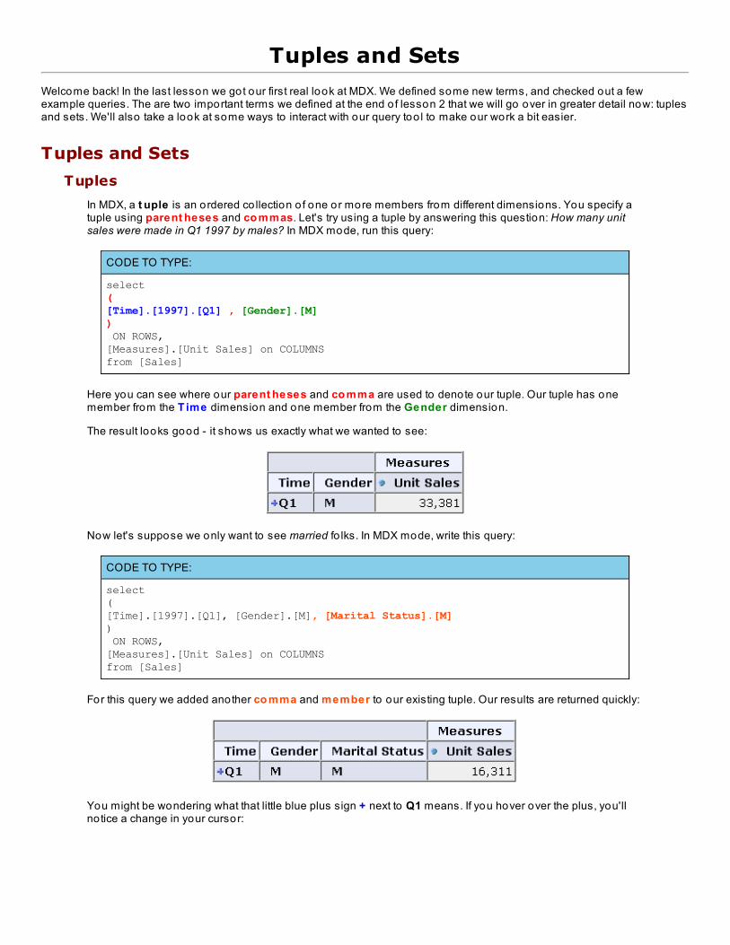
Some hierarchies have a special All member. This member allows you to calculate percentages versesto tals. We'll learn more about this later. In the Gender dimension in our data warehouse, the hierarchy lookslike this and includes the All member:
Members can also have properties. Many dimensions (like customers) usually have ID or key fields that tiedata back to source systems. These fields are not useful to most business users, but they may be o f interestto some.
The last two data sets are very important - so important we will cover them in detail in the next lesson. Theyare:
T uple - an ordered co llection o f one or more members from different dimensions.Set - an ordered co llection o f tuples with the same dimensionality.
We've only just begun to cover MDX. In the next lesson we'll learn more about tuples and sets, and start writing ourown MDX queries from scratch. See you there shortly!
Copyright © 1998-2014 O'Reilly Media, Inc.
This work is licensed under a Creative Commons Attribution-ShareAlike 3.0 Unported License.See http://creativecommons.org/licenses/by-sa/3.0/legalcode for more information.
Tuples and Sets
Welcome back! In the last lesson we got our first real look at MDX. We defined some new terms, and checked out a fewexample queries. The are two important terms we defined at the end o f lesson 2 that we will go over in greater detail now: tuplesand sets. We'll also take a look at some ways to interact with our query too l to make our work a bit easier.
Tuples and Sets
Tuples
In MDX, a t uple is an ordered co llection o f one or more members from different dimensions. You specify atuple using parent heses and co mmas. Let's try using a tuple by answering this question: How many unitsales were made in Q1 1997 by males? In MDX mode, run this query:
CODE TO TYPE:
select ([Time].[1997].[Q1] , [Gender].[M]) ON ROWS,[Measures].[Unit Sales] on COLUMNSfrom [Sales]
Here you can see where our parent heses and co mma are used to denote our tuple. Our tuple has onemember from the T ime dimension and one member from the Gender dimension.
The result looks good - it shows us exactly what we wanted to see:
Now let's suppose we only want to see married fo lks. In MDX mode, write this query:
CODE TO TYPE:
select ([Time].[1997].[Q1], [Gender].[M], [Marital Status].[M]) ON ROWS,[Measures].[Unit Sales] on COLUMNSfrom [Sales]
For this query we added another co mma and member to our existing tuple. Our results are returned quickly:
You might be wondering what that little blue plus sign + next to Q1 means. If you hover over the plus, you'llno tice a change in your cursor:
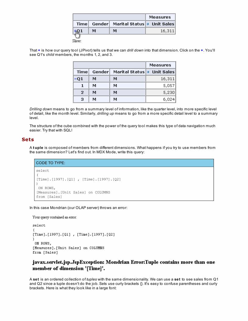
That + is how our query too l (JPivot) tells us that we can drill down into that dimension. Click on the + . You'llsee Q1's child members, the months 1, 2, and 3.
Drilling down means to go from a summary level o f information, like the quarter level, into more specific levelo f detail, like the month level. Similarly, drilling up means to go from a more specific detail level to a summarylevel.
The structure o f the cube combined with the power o f the query too l makes this type o f data navigation mucheasier. Try that with SQL!
Sets
A t uple is composed o f members from different dimensions. What happens if you try to use members fromthe same dimension? Let's find out. In MDX Mode, write this query:
CODE TO TYPE:
select ([Time].[1997].[Q1] , [Time].[1997].[Q2]) ON ROWS,[Measures].[Unit Sales] on COLUMNSfrom [Sales]
In this case Mondrian (our OLAP server) throws an error:
A set is an ordered co llection o f tuples with the same dimensionality. We can use a set to see sales from Q1and Q2 since a tuple doesn't do the job. Sets use curly brackets {}. It's easy to confuse parentheses and curlybrackets. Here is what they look like in a large font:
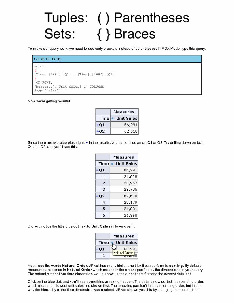
To make our query work, we need to use curly brackets instead o f parentheses. In MDX Mode, type this query:
CODE TO TYPE:
select {[Time].[1997].[Q1] , [Time].[1997].[Q2]} ON ROWS,[Measures].[Unit Sales] on COLUMNSfrom [Sales]
Now we're getting results!
Since there are two blue plus signs + in the results, you can drill down on Q1 or Q2. Try drilling down on bothQ1 and Q2, and you'll see this:
Did you notice the little blue dot next to Unit Sales? Hover over it:
You'll see the words Nat ural Order. JPivot has many tricks; one trick it can perform is so rt ing. By default,measures are sorted in Nat ural Order which means in the order specified by the dimensions in your query.The natural o rder o f our time dimension would show us the o ldest data first and the newest data last.
Click on the blue dot, and you'll see something amazing happen. The data is now sorted in ascending order,which means the lowest unit sales are shown first. The amazing part isn't in the ascending order, but in theway the hierarchy o f the time dimension was retained. JPivot shows you this by changing the blue dot to a
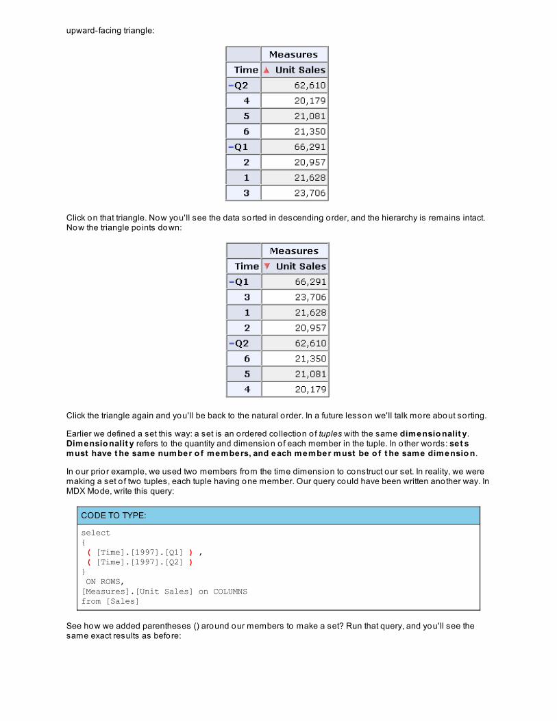
upward-facing triangle:
Click on that triangle. Now you'll see the data sorted in descending order, and the hierarchy is remains intact.Now the triangle po ints down:
Click the triangle again and you'll be back to the natural o rder. In a future lesson we'll talk more about sorting.
Earlier we defined a set this way: a set is an ordered co llection o f tuples with the same dimensio nalit y.Dimensio nalit y refers to the quantity and dimension o f each member in the tuple. In o ther words: set smust have t he same number o f members, and each member must be o f t he same dimensio n.
In our prio r example, we used two members from the time dimension to construct our set. In reality, we weremaking a set o f two tuples, each tuple having one member. Our query could have been written another way. InMDX Mode, write this query:
CODE TO TYPE:
select { ( [Time].[1997].[Q1] ) , ( [Time].[1997].[Q2] )} ON ROWS,[Measures].[Unit Sales] on COLUMNSfrom [Sales]
See how we added parentheses () around our members to make a set? Run that query, and you'll see thesame exact results as before:
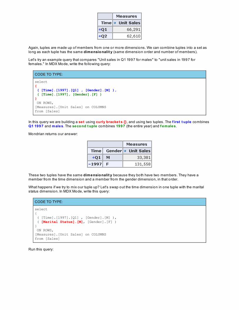
Again, tuples are made up o f members from one or more dimensions. We can combine tuples into a set aslong as each tuple has the same dimensio nalit y (same dimension order and number o f members).
Let's try an example query that compares "Unit sales in Q1 1997 for males" to "unit sales in 1997 forfemales." In MDX Mode, write the fo llowing query:
CODE TO TYPE:
select { ( [Time].[1997].[Q1] , [Gender].[M] ), ( [Time].[1997], [Gender].[F] )} ON ROWS,[Measures].[Unit Sales] on COLUMNSfrom [Sales]
In this query we are building a set using curly bracket s {} , and using two tuples. The f irst t uple combinesQ1 1997 and males. The seco nd t uple combines 1997 (the entire year) and f emales.
Mondrian returns our answer:
These two tuples have the same dimensio nalit y because they both have two members. They have amember from the time dimension and a member from the gender dimension, in that order.
What happens if we try to mix our tuple up? Let's swap out the time dimension in one tuple with the maritalstatus dimension. In MDX Mode, write this query:
CODE TO TYPE:
select { ( [Time].[1997].[Q1] , [Gender].[M] ), ( [Marital Status].[M], [Gender].[F] )} ON ROWS,[Measures].[Unit Sales] on COLUMNSfrom [Sales]
Run this query:
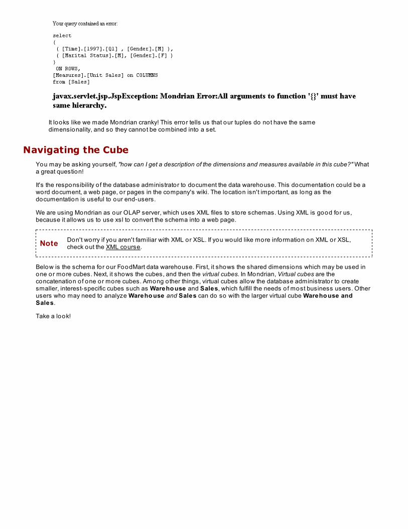
It looks like we made Mondrian cranky! This error tells us that our tuples do not have the samedimensionality, and so they cannot be combined into a set.
Navigating the CubeYou may be asking yourself, "how can I get a description of the dimensions and measures available in this cube?" Whata great question!
It's the responsibility o f the database administrator to document the data warehouse. This documentation could be aword document, a web page, or pages in the company's wiki. The location isn't important, as long as thedocumentation is useful to our end-users.
We are using Mondrian as our OLAP server, which uses XML files to store schemas. Using XML is good for us,because it allows us to use xsl to convert the schema into a web page.
Note Don't worry if you aren't familiar with XML or XSL. If you would like more information on XML or XSL,check out the XML course.
Below is the schema for our FoodMart data warehouse. First, it shows the shared dimensions which may be used inone or more cubes. Next, it shows the cubes, and then the virtual cubes. In Mondrian, Virtual cubes are theconcatenation o f one or more cubes. Among o ther things, virtual cubes allow the database administrator to createsmaller, interest-specific cubes such as Wareho use and Sales, which fulfill the needs o f most business users. Otherusers who may need to analyze Wareho use and Sales can do so with the larger virtual cube Wareho use andSales.
Take a look!
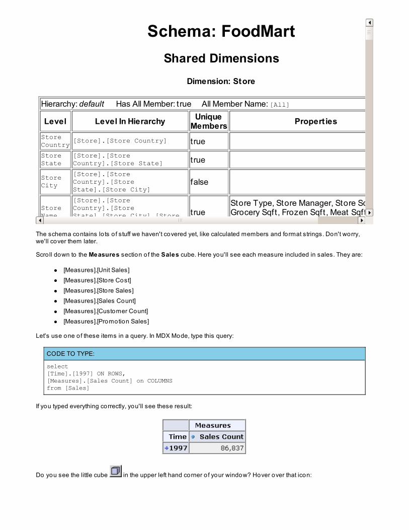
Schema: FoodMartShared Dimensions
Dimension: Store
Hierarchy: default Has All Member: t rue All Member Name: [All]
Level Level In Hierarchy UniqueMembers Propert ies
StoreCountry [Store].[Store Country] t rue StoreState
[Store].[StoreCountry].[Store State] t rue
StoreCity
[Store].[StoreCountry].[StoreState].[Store City]
false
StoreName
[Store].[StoreCountry].[StoreState].[Store City].[Store t rue
Store Type, Store Manager, Store Sqft ,Grocery Sqft , Frozen Sqft , Meat Sqft , Has
The schema contains lo ts o f stuff we haven't covered yet, like calculated members and format strings. Don't worry,we'll cover them later.
Scro ll down to the Measures section o f the Sales cube. Here you'll see each measure included in sales. They are:
[Measures].[Unit Sales][Measures].[Store Cost][Measures].[Store Sales][Measures].[Sales Count][Measures].[Customer Count][Measures].[Promotion Sales]
Let's use one o f these items in a query. In MDX Mode, type this query:
CODE TO TYPE:
select [Time].[1997] ON ROWS,[Measures].[Sales Count] on COLUMNSfrom [Sales]
If you typed everything correctly, you'll see these result:
Do you see the little cube in the upper left hand corner o f your window? Hover over that icon:
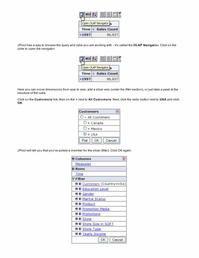
JPivot has a way to browse the query and cube you are working with - it's called the OLAP Navigat o r. Click on thecube to open the navigator:
Here you can move dimensions from axis to axis, add a slicer axis (under the filter section), o r just take a peek at thestructure o f the cube.
Click on the Cust o mers link, then on the next to All Cust o mers. Next, click the radio button next to USA and clickOK:
JPivot will tell you that you've picked a member for the slicer (filter). Click OK again:
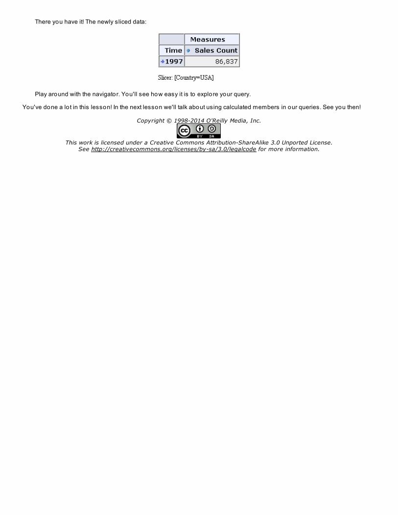
There you have it! The newly sliced data:
Play around with the navigator. You'll see how easy it is to explore your query.
You've done a lo t in this lesson! In the next lesson we'll talk about using calculated members in our queries. See you then!
Copyright © 1998-2014 O'Reilly Media, Inc.
This work is licensed under a Creative Commons Attribution-ShareAlike 3.0 Unported License.See http://creativecommons.org/licenses/by-sa/3.0/legalcode for more information.
Calculated Members
In the last lesson we took a look at the schema of our data warehouse, and we saw that the cube we've been working with hadseveral calculated members. In this lesson we're go ing to learn all about those calculated members.
Calculated MembersData warehouses usually contain a lo t o f information, but it is impossible to calculate and store every possibleassembly o f data. Sometimes data isn't stored anywhere - profit, fo r example, is usually calculated as costs subtractedfrom sales. Some users may only want to see pro fit fo r 1997, while o thers might want to see pro fit according to store.Enumerating, calculating, and storing all combinations o f dimensions, sales, and costs would take entirely too muchspace and effort.
Let's try to calculate pro fit (sales minus costs) in a query. It seems like we should be able to write a query using[Measures].[Store Sales] - [Measures].[Store Cost] in order to come up with pro fit. Let's try it. In MDXMode, write the fo llowing query:
CODE TO TYPE:
select [Time].[1997] ON ROWS,[Measures].[Store Sales] - [Measures].[Store Cost] on COLUMNSfrom [Sales]
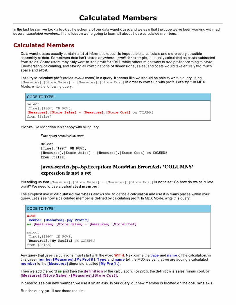
It looks like Mondrian isn't happy with our query:
It is telling us that [Measures].[Store Sales] - [Measures].[Store Cost] is not a set. So how do we calculatepro fit? We need to use a calculat ed member.
The simplest use o f calculat ed members allows you to define a calculation and use it in many places within yourquery. Let's see how a calculated member is defined by calculating pro fit. In MDX Mode, write this query:
CODE TO TYPE:
WITH member [Measures].[My Profit]as [Measures].[Store Sales] - [Measures].[Store Cost] select [Time].[1997] ON ROWS,[Measures].[My Profit] on COLUMNSfrom [Sales]
Any query that uses calculations must start with the word WIT H. Next come the t ype and name o f the calculation, inthis case member [Measures].[My Pro f it ] . T ype and name tell the MDX server that we are adding a calculatedmember to the [Measures] dimension, called [My Pro f it ] .
Then we add the word as and then the def init io n o f the calculation. For profit, the definition is sales minus cost, o r[Measures].[St o re Sales] - [Measures].[St o re Co st ] .
In order to see our new member, we use it on an axis. In our query, our new member is located on the co lumns axis.
Run the query, you'll see these results:
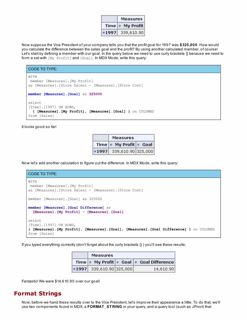
Now suppose the Vice President o f your company tells you that the pro fit goal fo r 1997 was $325,000 . How wouldyou calculate the difference between the sales goal and the pro fit? By using another calculated member, o f course!Let's start by defining a member with our goal. In the query below we need to use curly brackets {} because we need toform a set with [My Profit] and [Goal]. In MDX Mode, write this query:
CODE TO TYPE:
WITH member [Measures].[My Profit]as [Measures].[Store Sales] - [Measures].[Store Cost]
member [Measures].[Goal] as 325000 select [Time].[1997] ON ROWS, { [Measures].[My Profit], [Measures].[Goal] } on COLUMNSfrom [Sales]
It looks good so far!
Now let's add another calculation to figure out the difference. In MDX Mode, write this query:
CODE TO TYPE:
WITH member [Measures].[My Profit]as [Measures].[Store Sales] - [Measures].[Store Cost]
member [Measures].[Goal] as 325000
member [Measures].[Goal Difference] as [Measures].[My Profit] - [Measures].[Goal] select [Time].[1997] ON ROWS,{ [Measures].[My Profit], [Measures].[Goal], [Measures].[Goal Difference] } on COLUMNSfrom [Sales]
If you typed everything correctly (don't fo rget about the curly brackets {} ) you'll see these results:
Fantastic! We were $14,610.90 over our goal!
Format StringsNow, before we hand these results over to the Vice President, let's improve their appearance a little. To do that, we'lluse two components found in MDX: a FORMAT _ST RING in your query, and a query too l (such as JPivot) that
supports parsing and displaying format strings.
Format strings work on string, numeric, o r date values. Format strings allow you to convert string text to uppercase,lowercase, and even handle special cases such as NULLs or empty strings. Format strings allow you to formatnumbers any way you'd like, and handle positive, negative, zero , and empty values differently.
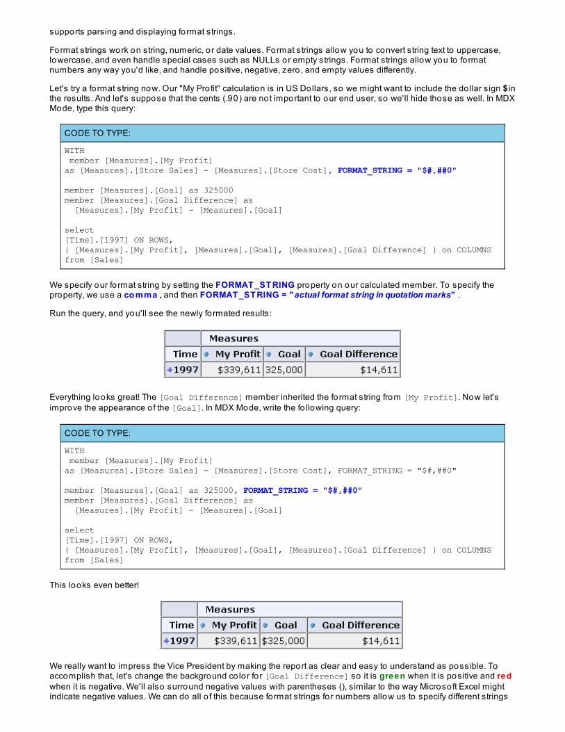
Let's try a format string now. Our "My Profit" calculation is in US Dollars, so we might want to include the do llar sign $ inthe results. And let's suppose that the cents (.90) are not important to our end user, so we'll hide those as well. In MDXMode, type this query:
CODE TO TYPE:
WITH member [Measures].[My Profit] as [Measures].[Store Sales] - [Measures].[Store Cost], FORMAT_STRING = "$#,##0"
member [Measures].[Goal] as 325000member [Measures].[Goal Difference] as [Measures].[My Profit] - [Measures].[Goal] select [Time].[1997] ON ROWS,{ [Measures].[My Profit], [Measures].[Goal], [Measures].[Goal Difference] } on COLUMNSfrom [Sales]
We specify our fo rmat string by setting the FORMAT _ST RING property on our calculated member. To specify theproperty, we use a co mma , and then FORMAT _ST RING = "actual format string in quotation marks" .
Run the query, and you'll see the newly formated results:
Everything looks great! The [Goal Difference] member inherited the format string from [My Profit]. Now let'simprove the appearance o f the [Goal]. In MDX Mode, write the fo llowing query:
CODE TO TYPE:
WITH member [Measures].[My Profit] as [Measures].[Store Sales] - [Measures].[Store Cost], FORMAT_STRING = "$#,##0"
member [Measures].[Goal] as 325000, FORMAT_STRING = "$#,##0"member [Measures].[Goal Difference] as [Measures].[My Profit] - [Measures].[Goal] select [Time].[1997] ON ROWS,{ [Measures].[My Profit], [Measures].[Goal], [Measures].[Goal Difference] } on COLUMNSfrom [Sales]
This looks even better!
We really want to impress the Vice President by making the report as clear and easy to understand as possible. Toaccomplish that, let's change the background co lor fo r [Goal Difference] so it is green when it is positive and redwhen it is negative. We'll also surround negative values with parentheses (), similar to the way Microsoft Excel mightindicate negative values. We can do all o f this because format strings for numbers allow us to specify different strings
fo r positive and negative values (as well as zero and empty values).
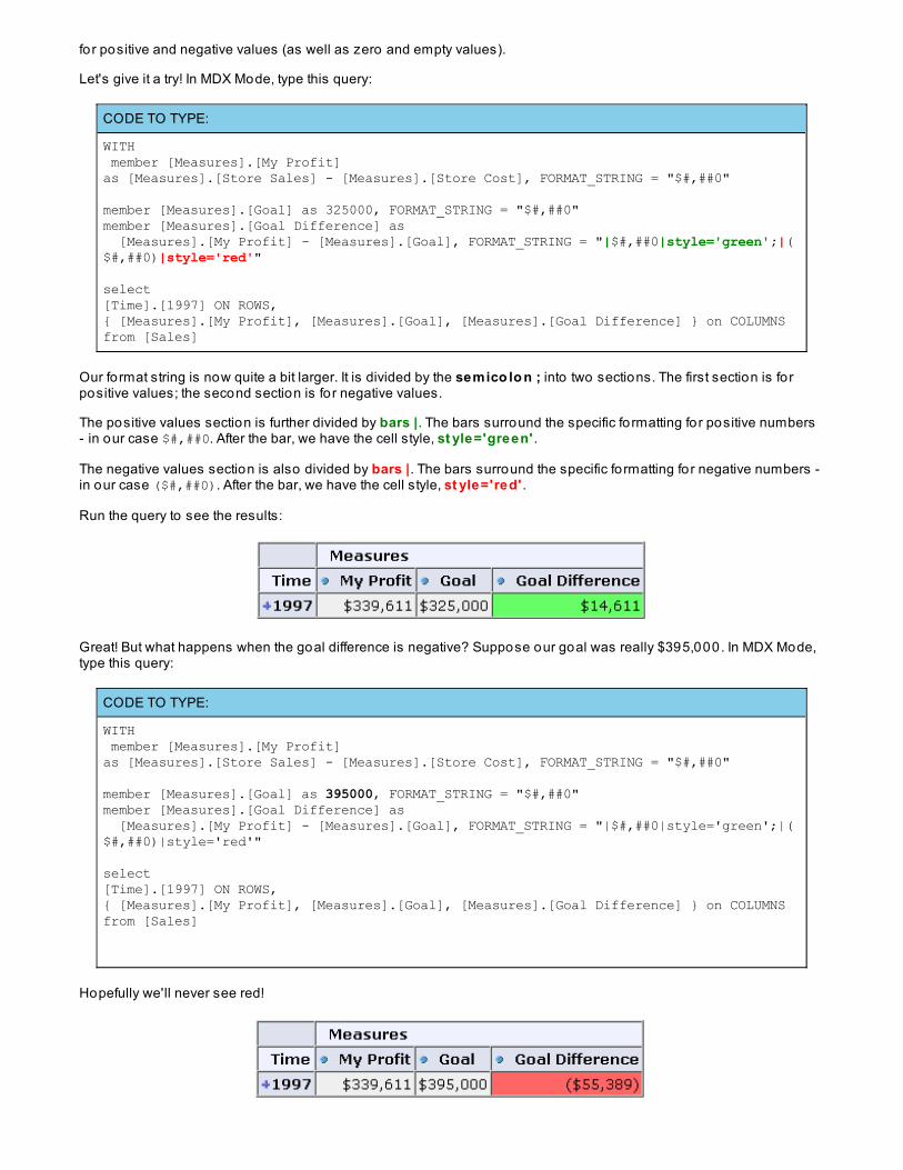
Let's give it a try! In MDX Mode, type this query:
CODE TO TYPE:
WITH member [Measures].[My Profit] as [Measures].[Store Sales] - [Measures].[Store Cost], FORMAT_STRING = "$#,##0"
member [Measures].[Goal] as 325000, FORMAT_STRING = "$#,##0"member [Measures].[Goal Difference] as [Measures].[My Profit] - [Measures].[Goal], FORMAT_STRING = "|$#,##0|style='green';|($#,##0)|style='red'" select [Time].[1997] ON ROWS,{ [Measures].[My Profit], [Measures].[Goal], [Measures].[Goal Difference] } on COLUMNSfrom [Sales]
Our format string is now quite a bit larger. It is divided by the semico lo n ; into two sections. The first section is fo rpositive values; the second section is fo r negative values.
The positive values section is further divided by bars |. The bars surround the specific fo rmatting for positive numbers- in our case $#,##0. After the bar, we have the cell style, st yle='green' .
The negative values section is also divided by bars |. The bars surround the specific fo rmatting for negative numbers -in our case ($#,##0). After the bar, we have the cell style, st yle='red' .
Run the query to see the results:
Great! But what happens when the goal difference is negative? Suppose our goal was really $395,000. In MDX Mode,type this query:
CODE TO TYPE:
WITH member [Measures].[My Profit] as [Measures].[Store Sales] - [Measures].[Store Cost], FORMAT_STRING = "$#,##0"
member [Measures].[Goal] as 395000, FORMAT_STRING = "$#,##0"member [Measures].[Goal Difference] as [Measures].[My Profit] - [Measures].[Goal], FORMAT_STRING = "|$#,##0|style='green';|($#,##0)|style='red'" select [Time].[1997] ON ROWS,{ [Measures].[My Profit], [Measures].[Goal], [Measures].[Goal Difference] } on COLUMNSfrom [Sales]
Hopefully we'll never see red!
For more information on format strings, check out Microsoft's SQL Server 2008 web site. Our OLAP server, Mondrian,doesn't support everything that SQL Server 2008 does, but most o f the information is relevant.
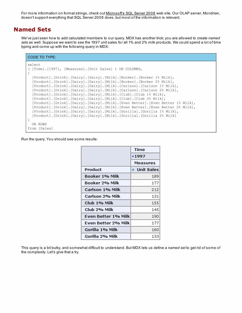
Named SetsWe've just seen how to add calculated members to our query. MDX has another trick; you are allowed to create namedsets as well. Suppose we want to see the 1997 unit sales for all 1% and 2% milk products. We could spend a lo t o f timetyping and come up with the fo llowing query in MDX:
CODE TO TYPE:
select( [Time].[1997], [Measures].[Unit Sales] ) ON COLUMNS,{ [Product].[Drink].[Dairy].[Dairy].[Milk].[Booker].[Booker 1% Milk], [Product].[Drink].[Dairy].[Dairy].[Milk].[Booker].[Booker 2% Milk], [Product].[Drink].[Dairy].[Dairy].[Milk].[Carlson].[Carlson 1% Milk], [Product].[Drink].[Dairy].[Dairy].[Milk].[Carlson].[Carlson 2% Milk], [Product].[Drink].[Dairy].[Dairy].[Milk].[Club].[Club 1% Milk], [Product].[Drink].[Dairy].[Dairy].[Milk].[Club].[Club 2% Milk], [Product].[Drink].[Dairy].[Dairy].[Milk].[Even Better].[Even Better 1% Milk], [Product].[Drink].[Dairy].[Dairy].[Milk].[Even Better].[Even Better 2% Milk], [Product].[Drink].[Dairy].[Dairy].[Milk].[Gorilla].[Gorilla 1% Milk], [Product].[Drink].[Dairy].[Dairy].[Milk].[Gorilla].[Gorilla 2% Milk]} ON ROWSfrom [Sales]
Run the query. You should see some results:
This query is a bit bulky, and somewhat difficult to understand. But MDX lets us define a named set to get rid o f some ofthe complexity. Let's give that a try.
CODE TO TYPE:
WITH set [1% and 2% Milk]as{ [Product].[Drink].[Dairy].[Dairy].[Milk].[Booker].[Booker 1% Milk], [Product].[Drink].[Dairy].[Dairy].[Milk].[Booker].[Booker 2% Milk], [Product].[Drink].[Dairy].[Dairy].[Milk].[Carlson].[Carlson 1% Milk], [Product].[Drink].[Dairy].[Dairy].[Milk].[Carlson].[Carlson 2% Milk], [Product].[Drink].[Dairy].[Dairy].[Milk].[Club].[Club 1% Milk], [Product].[Drink].[Dairy].[Dairy].[Milk].[Club].[Club 2% Milk], [Product].[Drink].[Dairy].[Dairy].[Milk].[Even Better].[Even Better 1% Milk], [Product].[Drink].[Dairy].[Dairy].[Milk].[Even Better].[Even Better 2% Milk], [Product].[Drink].[Dairy].[Dairy].[Milk].[Gorilla].[Gorilla 1% Milk], [Product].[Drink].[Dairy].[Dairy].[Milk].[Gorilla].[Gorilla 2% Milk]} select( [Time].[1997], [Measures].[Unit Sales] ) ON COLUMNS, [1% and 2% Milk] ON ROWSfrom [Sales]
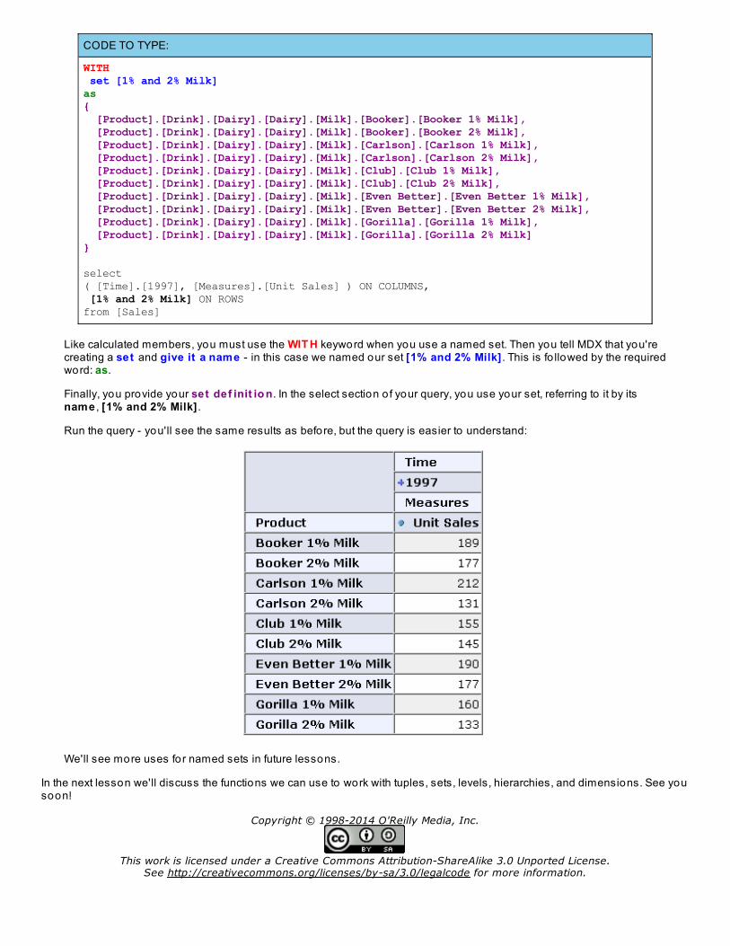
Like calculated members, you must use the WIT H keyword when you use a named set. Then you tell MDX that you'recreating a set and give it a name - in this case we named our set [1% and 2% Milk] . This is fo llowed by the requiredword: as.
Finally, you provide your set def init io n. In the select section o f your query, you use your set, referring to it by itsname , [1% and 2% Milk] .
Run the query - you'll see the same results as before, but the query is easier to understand:
We'll see more uses for named sets in future lessons.
In the next lesson we'll discuss the functions we can use to work with tuples, sets, levels, hierarchies, and dimensions. See yousoon!
Copyright © 1998-2014 O'Reilly Media, Inc.
This work is licensed under a Creative Commons Attribution-ShareAlike 3.0 Unported License.See http://creativecommons.org/licenses/by-sa/3.0/legalcode for more information.
MDX Functions, Part I
Welcome back! In the last lesson we took a look at tuples and sets. In this lesson we'll take a look at MDX functions we can useto make our queries easier.
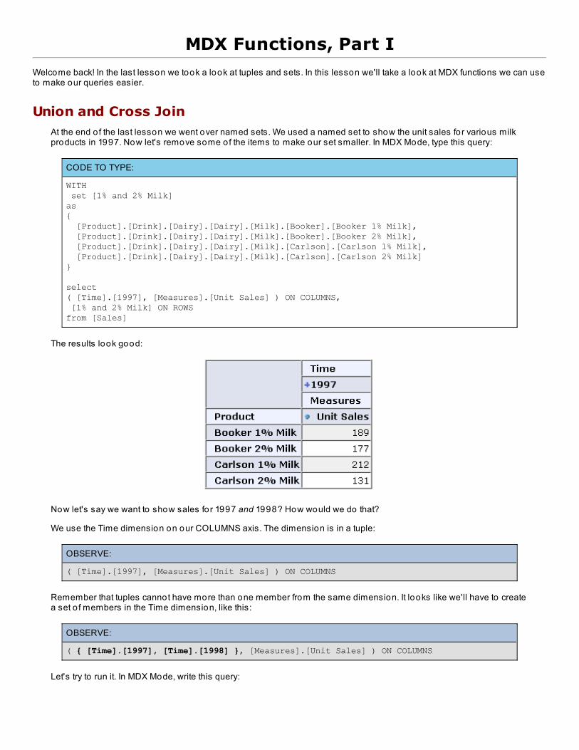
Union and Cross JoinAt the end o f the last lesson we went over named sets. We used a named set to show the unit sales for various milkproducts in 1997. Now let's remove some of the items to make our set smaller. In MDX Mode, type this query:
CODE TO TYPE:
WITH set [1% and 2% Milk]as{ [Product].[Drink].[Dairy].[Dairy].[Milk].[Booker].[Booker 1% Milk], [Product].[Drink].[Dairy].[Dairy].[Milk].[Booker].[Booker 2% Milk], [Product].[Drink].[Dairy].[Dairy].[Milk].[Carlson].[Carlson 1% Milk], [Product].[Drink].[Dairy].[Dairy].[Milk].[Carlson].[Carlson 2% Milk]} select( [Time].[1997], [Measures].[Unit Sales] ) ON COLUMNS, [1% and 2% Milk] ON ROWSfrom [Sales]
The results look good:
Now let's say we want to show sales for 1997 and 1998? How would we do that?
We use the Time dimension on our COLUMNS axis. The dimension is in a tuple:
OBSERVE:
( [Time].[1997], [Measures].[Unit Sales] ) ON COLUMNS
Remember that tuples cannot have more than one member from the same dimension. It looks like we'll have to createa set o f members in the Time dimension, like this:
OBSERVE:
( { [Time].[1997], [Time].[1998] }, [Measures].[Unit Sales] ) ON COLUMNS
Let's try to run it. In MDX Mode, write this query:
CODE TO TYPE:
WITH set [1% and 2% Milk]as{ [Product].[Drink].[Dairy].[Dairy].[Milk].[Booker].[Booker 1% Milk], [Product].[Drink].[Dairy].[Dairy].[Milk].[Booker].[Booker 2% Milk], [Product].[Drink].[Dairy].[Dairy].[Milk].[Carlson].[Carlson 1% Milk], [Product].[Drink].[Dairy].[Dairy].[Milk].[Carlson].[Carlson 2% Milk]} select( { [Time].[1997], [Time].[1998] }, [Measures].[Unit Sales] ) ON COLUMNS, [1% and 2% Milk] ON ROWSfrom [Sales]
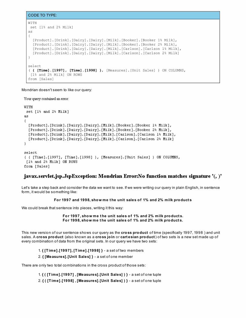
Mondrian doesn't seem to like our query:
Let's take a step back and consider the data we want to see. If we were writing our query in plain English, in sentenceform, it would be something like:
Fo r 1997 and 1998, sho w me t he unit sales o f 1% and 2% milk pro duct s
We could break that sentence into pieces, writing it this way:
Fo r 1997, sho w me t he unit sales o f 1% and 2% milk pro duct s.Fo r 1998, sho w me t he unit sales o f 1% and 2% milk pro duct s.
This new version o f our sentence shows our query as the cro ss pro duct o f time (specifically 1997, 1998 ) and unitsales. A cro ss pro duct (also known as a cro ss jo in o r cart esian pro duct ) o f two sets is a new set made up o fevery combination o f data from the original sets. In our query we have two sets:
1. { [T ime].[1997], [T ime].[1998] } - a set o f two members2. { [Measures].[Unit Sales] } - a set o f one member
There are only two to tal combinations in the cross product o f those sets:
1. { ( [T ime].[1997] , [Measures].[Unit Sales] ) } - a set o f one tuple2. { ( [T ime].[1998] , [Measures].[Unit Sales] ) } - a set o f one tuple
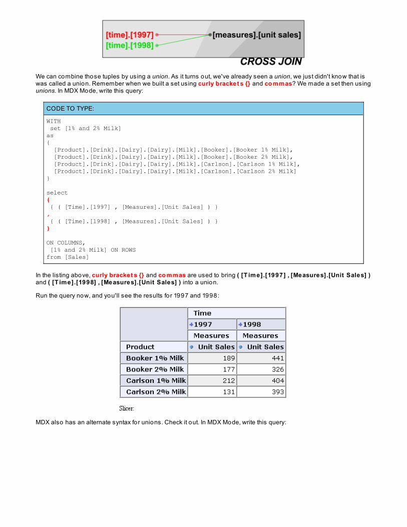
We can combine those tuples by using a union. As it turns out, we've already seen a union, we just didn't know that iswas called a union. Remember when we built a set using curly bracket s {} and co mmas? We made a set then usingunions. In MDX Mode, write this query:
CODE TO TYPE:
WITH set [1% and 2% Milk]as{ [Product].[Drink].[Dairy].[Dairy].[Milk].[Booker].[Booker 1% Milk], [Product].[Drink].[Dairy].[Dairy].[Milk].[Booker].[Booker 2% Milk], [Product].[Drink].[Dairy].[Dairy].[Milk].[Carlson].[Carlson 1% Milk], [Product].[Drink].[Dairy].[Dairy].[Milk].[Carlson].[Carlson 2% Milk]} select{ { ( [Time].[1997] , [Measures].[Unit Sales] ) }, { ( [Time].[1998] , [Measures].[Unit Sales] ) }}
ON COLUMNS, [1% and 2% Milk] ON ROWSfrom [Sales]
In the listing above, curly bracket s {} and co mmas are used to bring ( [T ime].[1997] , [Measures].[Unit Sales] )and ( [T ime].[1998] , [Measures].[Unit Sales] ) into a union.
Run the query now, and you'll see the results fo r 1997 and 1998:
MDX also has an alternate syntax for unions. Check it out. In MDX Mode, write this query:
CODE TO TYPE:
WITH set [1% and 2% Milk]as{ [Product].[Drink].[Dairy].[Dairy].[Milk].[Booker].[Booker 1% Milk], [Product].[Drink].[Dairy].[Dairy].[Milk].[Booker].[Booker 2% Milk], [Product].[Drink].[Dairy].[Dairy].[Milk].[Carlson].[Carlson 1% Milk], [Product].[Drink].[Dairy].[Dairy].[Milk].[Carlson].[Carlson 2% Milk]} selectUNION ( { ( [Time].[1997] , [Measures].[Unit Sales] ) }, { ( [Time].[1998] , [Measures].[Unit Sales] ) })
ON COLUMNS, [1% and 2% Milk] ON ROWSfrom [Sales]
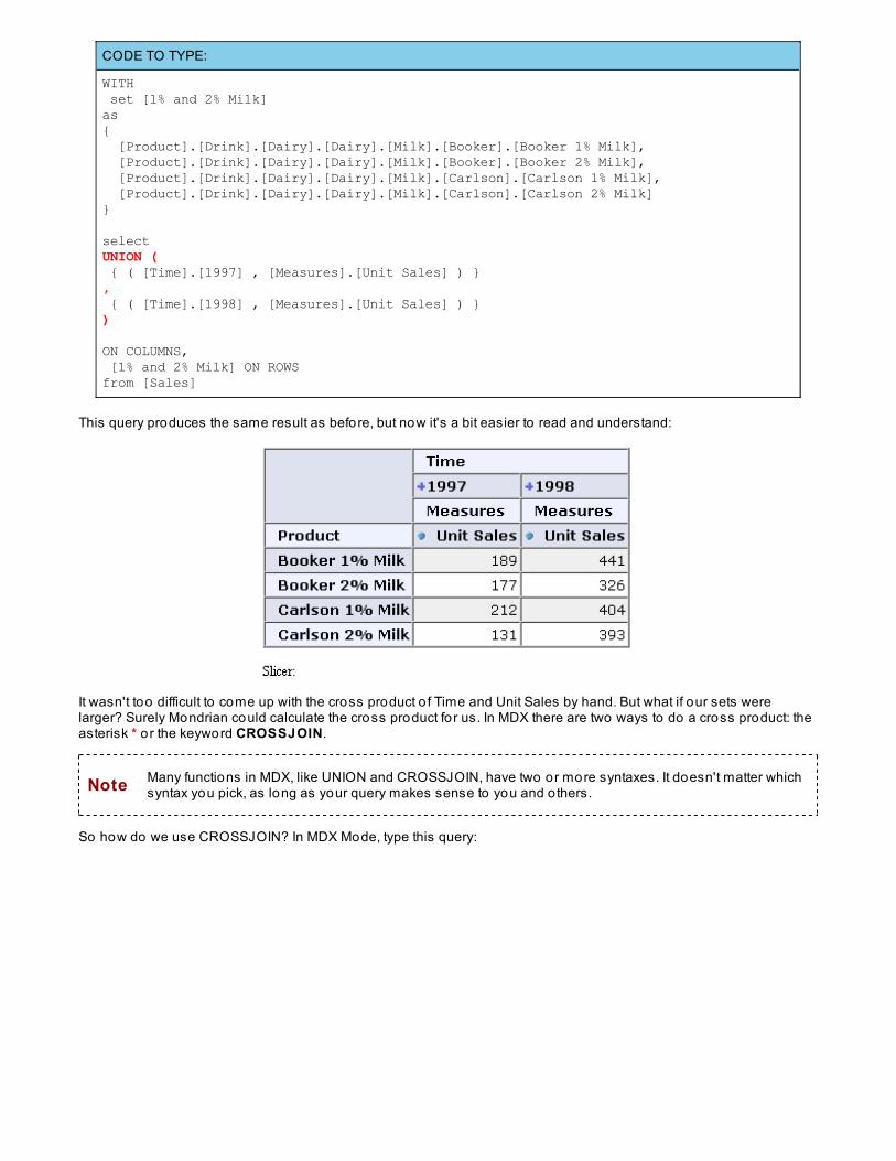
This query produces the same result as before, but now it's a bit easier to read and understand:
It wasn't too difficult to come up with the cross product o f Time and Unit Sales by hand. But what if our sets werelarger? Surely Mondrian could calculate the cross product fo r us. In MDX there are two ways to do a cross product: theasterisk * o r the keyword CROSSJOIN.
Note Many functions in MDX, like UNION and CROSSJOIN, have two or more syntaxes. It doesn't matter whichsyntax you pick, as long as your query makes sense to you and o thers.
So how do we use CROSSJOIN? In MDX Mode, type this query:

CODE TO TYPE:
WITH set [1% and 2% Milk]as{ [Product].[Drink].[Dairy].[Dairy].[Milk].[Booker].[Booker 1% Milk], [Product].[Drink].[Dairy].[Dairy].[Milk].[Booker].[Booker 2% Milk], [Product].[Drink].[Dairy].[Dairy].[Milk].[Carlson].[Carlson 1% Milk], [Product].[Drink].[Dairy].[Dairy].[Milk].[Carlson].[Carlson 2% Milk]} select
{ [Time].[1997], [Time].[1998] }* { [Measures].[Unit Sales] }
ON COLUMNS, [1% and 2% Milk] ON ROWSfrom [Sales]
In the code above, we use the asterisk * to calculate the cross jo in o f two sets: { [T ime].[1997], [T ime].[1998] } and{ [Measures].[Unit Sales] } .
Once again, our results look exactly the same, but this time our query is much shorter:
Other Set FunctionsNow suppose you wanted to break these sales down even further, according to gender. In previous lessons we usedthe [Gender] dimension in a query, and saw how its members were called [Gender].[M] and [Gender].[F]. Nowwe want a way to return the set o f all members from a specific level in a dimension. Fortunately, MDX has a specialfunction called Members that returns a set o f every member o f a dimension. Members can be used on a dimension,level, o r hierarchy. In MDX Mode, type this query:

CODE TO TYPE:
WITH set [1% and 2% Milk]as{ [Product].[Drink].[Dairy].[Dairy].[Milk].[Booker].[Booker 1% Milk], [Product].[Drink].[Dairy].[Dairy].[Milk].[Booker].[Booker 2% Milk], [Product].[Drink].[Dairy].[Dairy].[Milk].[Carlson].[Carlson 1% Milk], [Product].[Drink].[Dairy].[Dairy].[Milk].[Carlson].[Carlson 2% Milk]} select
{ [Time].[1997], [Time].[1998] }*[Gender].Members* { [Measures].[Unit Sales] }
ON COLUMNS, [1% and 2% Milk] ON ROWSfrom [Sales]
In this query we continue to use asterisks * to cross jo in our sets. And this time we've added a new set:[Gender].Members. This new set includes all members o f the [Gender] dimension.
Run the query and you'll see the newly augmented results:
We've seen the F and M members o f the gender dimension before, but where did the All Gender member comefrom? Mondrian allows schema authors to specify special All members for levels. This makes it possible to comparemembers against to tals fo r percentages.
So, what if we didn't want to see the All Member member? MDX has another function we can use, called Children.This function returns the set o f children o f a member. Let's try it! In MDX Mode, write the fo llowing query:
CODE TO TYPE:
WITH set [1% and 2% Milk]as{ [Product].[Drink].[Dairy].[Dairy].[Milk].[Booker].[Booker 1% Milk], [Product].[Drink].[Dairy].[Dairy].[Milk].[Booker].[Booker 2% Milk], [Product].[Drink].[Dairy].[Dairy].[Milk].[Carlson].[Carlson 1% Milk], [Product].[Drink].[Dairy].[Dairy].[Milk].[Carlson].[Carlson 2% Milk]} select
{ [Time].[1997], [Time].[1998] }*[Gender].Children* { [Measures].[Unit Sales] }
ON COLUMNS, [1% and 2% Milk] ON ROWSfrom [Sales]
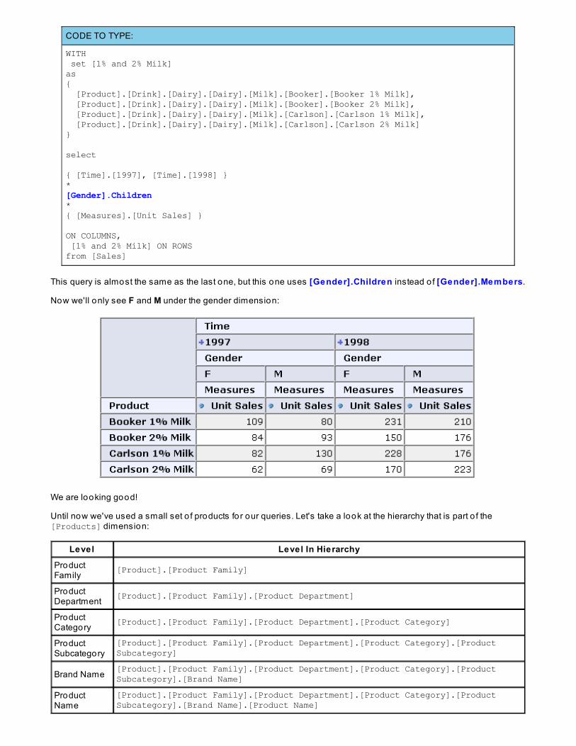
This query is almost the same as the last one, but this one uses [Gender].Children instead o f [Gender].Members.
Now we'll only see F and M under the gender dimension:
We are looking good!
Until now we've used a small set o f products for our queries. Let's take a look at the hierarchy that is part o f the[Products] dimension:
Level Level In Hierarchy
ProductFamily [Product].[Product Family]
ProductDepartment [Product].[Product Family].[Product Department]
ProductCategory [Product].[Product Family].[Product Department].[Product Category]
ProductSubcategory
[Product].[Product Family].[Product Department].[Product Category].[ProductSubcategory]
Brand Name [Product].[Product Family].[Product Department].[Product Category].[ProductSubcategory].[Brand Name]
ProductName
[Product].[Product Family].[Product Department].[Product Category].[ProductSubcategory].[Brand Name].[Product Name]
Here's the set we've used:
OBSERVE:
set [1% and 2% Milk]as{ [Product].[Drink].[Dairy].[Dairy].[Milk].[Booker].[Booker 1% Milk], [Product].[Drink].[Dairy].[Dairy].[Milk].[Booker].[Booker 2% Milk], [Product].[Drink].[Dairy].[Dairy].[Milk].[Carlson].[Carlson 1% Milk], [Product].[Drink].[Dairy].[Dairy].[Milk].[Carlson].[Carlson 2% Milk]}
All o f these members have the same [Product Subcategory] o f [Milk]. Each has a different [Brand Name] and[Product Name].
Suppose the Vice President wants to see 1997 and 1997 unit sales for all Milk products, according to gender. Howwould we answer that query? It would take a lo t o f time to look up each milk brand and product, and our named setwould become really large. Then to complicate matters further, each time our stores added a new milk brand, our querywould need to be updated. There has to be a better way!
We've already seen the Children function, so let's try to use it in our query. Type this in MDX Mode:
CODE TO TYPE:
WITH set [1% and 2% Milk]as[Product].[Drink].[Dairy].[Dairy].[Milk].Children select
{ [Time].[1997], [Time].[1998] }*[Gender].Children* { [Measures].[Unit Sales] }
ON COLUMNS, [1% and 2% Milk] ON ROWSfrom [Sales]
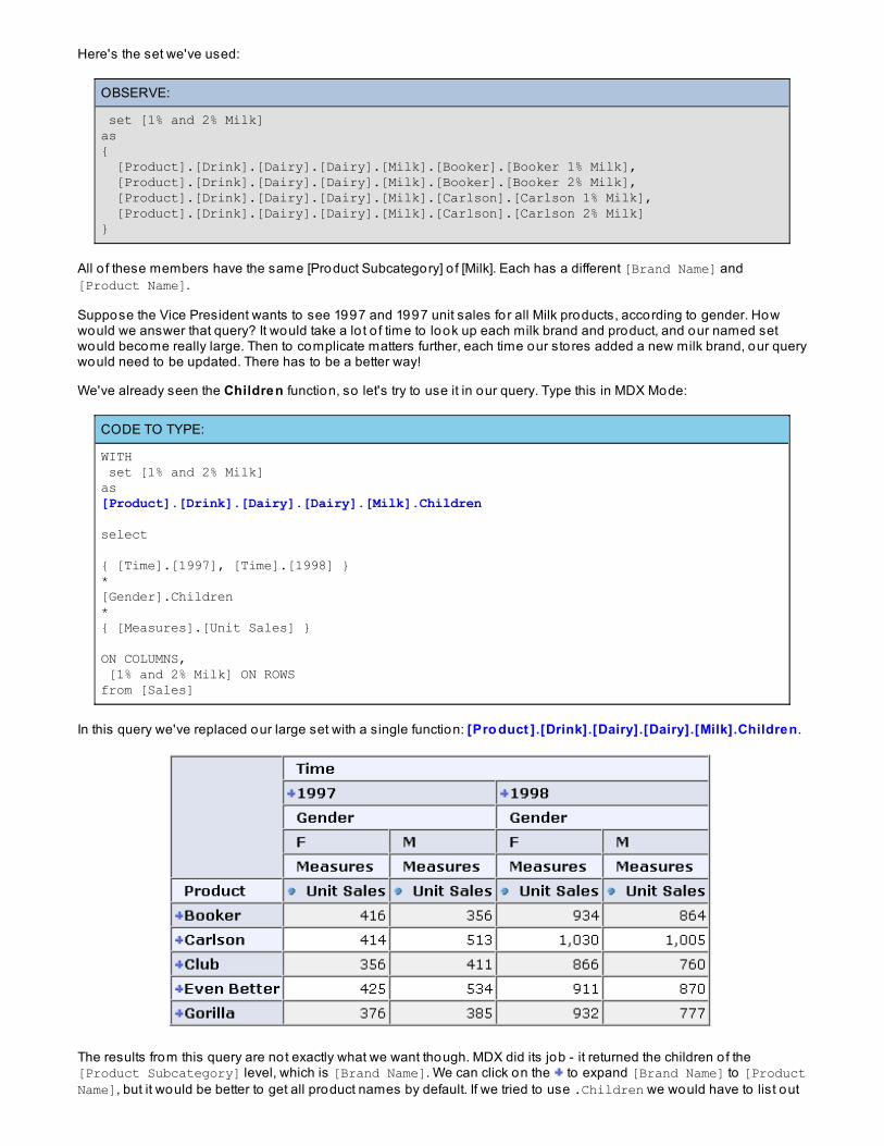
In this query we've replaced our large set with a single function: [Pro duct ].[Drink].[Dairy].[Dairy].[Milk].Children.
The results from this query are not exactly what we want though. MDX did its job - it returned the children o f the[Product Subcategory] level, which is [Brand Name]. We can click on the to expand [Brand Name] to [ProductName], but it would be better to get all product names by default. If we tried to use .Children we would have to list out

every [Brand Name] - something we are trying to avo id. There is a better way. MDX has a function calledDescendant s which can make short work o f this problem.
The Descendant s function returns a set o f all members at a given level. At first glance this seems exactly like theMembers o r Children function, but there is one major difference.
Children returns a set o f members below a specific member. In the last example it returned a set o f [Brand Name]sbelow the [Product Subcategory] level.
Descendant s returns a set o f members at a specific level, which are descendants (like children, grandchildren, greatgrandchildren, and so on) o f a specified level. Take a look. Type this query in MDX Mode:
CODE TO TYPE:
WITH set [1% and 2% Milk]as
Descendants( [Product].[Drink].[Dairy].[Dairy].[Milk],[Product].[Product Name]) select
{ [Time].[1997], [Time].[1998] }*[Gender].Children* { [Measures].[Unit Sales] }
ON COLUMNS, [1% and 2% Milk] ON ROWSfrom [Sales]
In this query we use the Descendant s function to get the descendants o f the member[Pro duct ].[Drink].[Dairy].[Dairy].[Milk] , at the [Pro duct ].[Pro duct Name] level.
When you run the query, you'll see the fo llowing results (actually you'll see more - this image only shows the first fewitems):
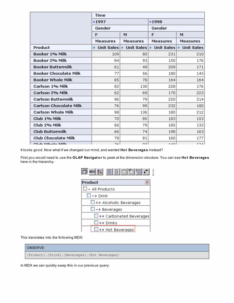
It looks good. Now what if we changed our mind, and wanted Ho t Beverages instead?
First you would need to use the OLAP Navigat o r to peek at the dimension structure. You can see Ho t Beverageshere in the hierarchy:
This translates into the fo llowing MDX:
OBSERVE:
[Product].[Drink].[Beverages].[Hot Beverages]
In MDX we can quickly swap this in our previous query:
CODE TO TYPE:
WITH set [Beverages]as
Descendants( [Product].[Drink].[Beverages].[Hot Beverages],[Product].[Product Name]) select
{ [Time].[1997], [Time].[1998] }*[Gender].Children* { [Measures].[Unit Sales] }
ON COLUMNS, [Beverages] ON ROWSfrom [Sales]
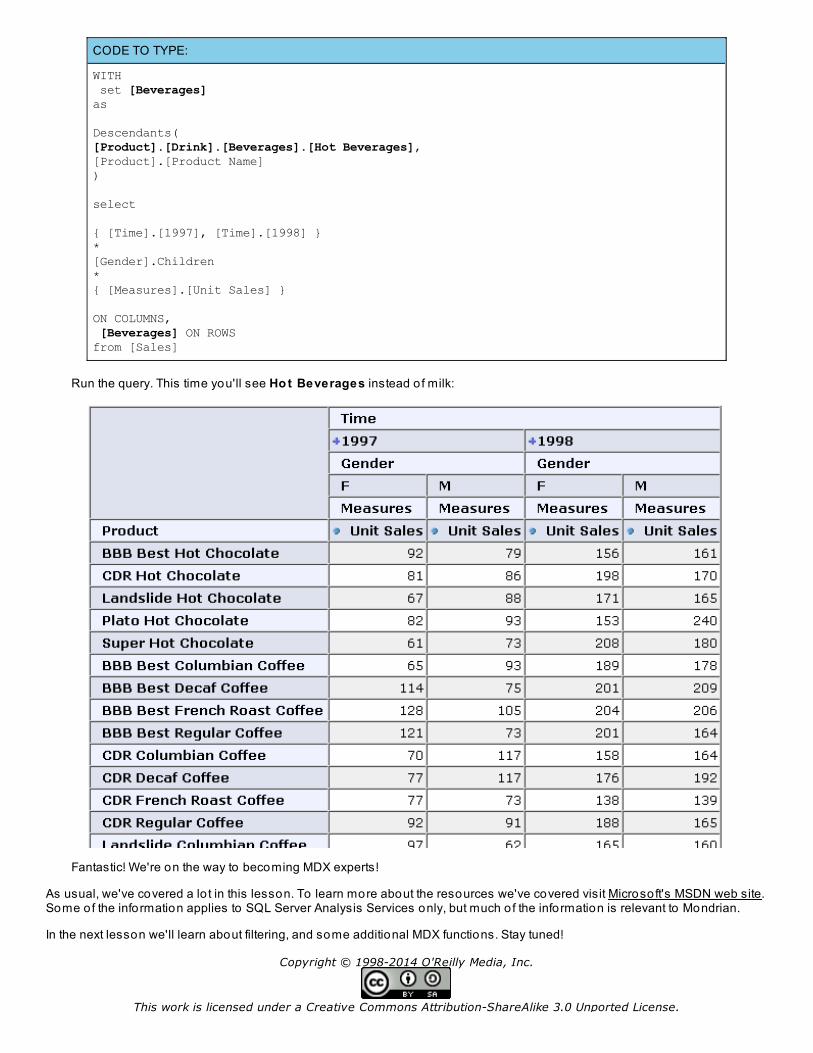
Run the query. This time you'll see Ho t Beverages instead o f milk:
Fantastic! We're on the way to becoming MDX experts!
As usual, we've covered a lo t in this lesson. To learn more about the resources we've covered visit Microsoft's MSDN web site.Some of the information applies to SQL Server Analysis Services only, but much o f the information is relevant to Mondrian.
In the next lesson we'll learn about filtering, and some additional MDX functions. Stay tuned!
Copyright © 1998-2014 O'Reilly Media, Inc.
This work is licensed under a Creative Commons Attribution-ShareAlike 3.0 Unported License.

This work is licensed under a Creative Commons Attribution-ShareAlike 3.0 Unported License.See http://creativecommons.org/licenses/by-sa/3.0/legalcode for more information.
MDX Functions, Part II
In the last lesson we learned how to use some powerful MDX functions. In this lesson we'll go over several more MDXfunctions, including the extremely powerful Filter function.
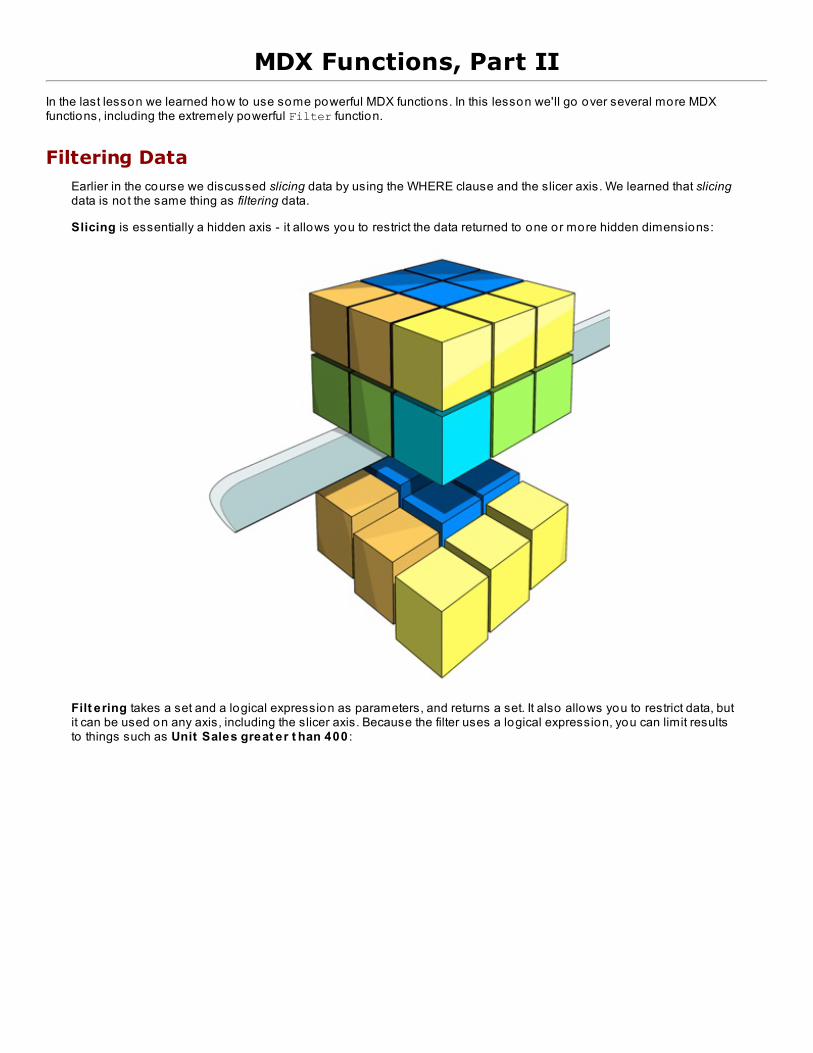
Filtering DataEarlier in the course we discussed slicing data by using the WHERE clause and the slicer axis. We learned that slicingdata is not the same thing as filtering data.
Slicing is essentially a hidden axis - it allows you to restrict the data returned to one or more hidden dimensions:
Filt ering takes a set and a logical expression as parameters, and returns a set. It also allows you to restrict data, butit can be used on any axis, including the slicer axis. Because the filter uses a logical expression, you can limit resultsto things such as Unit Sales great er t han 400 :
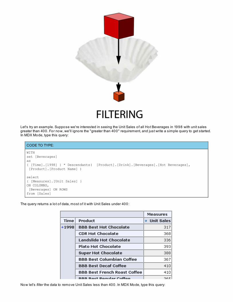
Let's try an example. Suppose we're interested in seeing the Unit Sales o f all Hot Beverages in 1998 with unit salesgreater than 400. For now, we'll ignore the "greater than 400" requirement, and just write a simple query to get started.In MDX Mode, type this query:
CODE TO TYPE:
WITHset [Beverages]as{ [Time].[1998] } * Descendants( [Product].[Drink].[Beverages].[Hot Beverages], [Product].[Product Name] )
select{ [Measures].[Unit Sales] }ON COLUMNS, [Beverages] ON ROWSfrom [Sales]
The query returns a lo t o f data, most o f it with Unit Sales under 400:
Now let's filter the data to remove Unit Sales less than 400. In MDX Mode, type this query:
CODE TO TYPE:
WITHset [Beverages]asFILTER({ [Time].[1998] } * Descendants( [Product].[Drink].[Beverages].[Hot Beverages], [Product].[Product Name] ),[Measures].[Unit Sales] > 400)select{ [Measures].[Unit Sales] }ON COLUMNS, [Beverages] ON ROWSfrom [Sales]
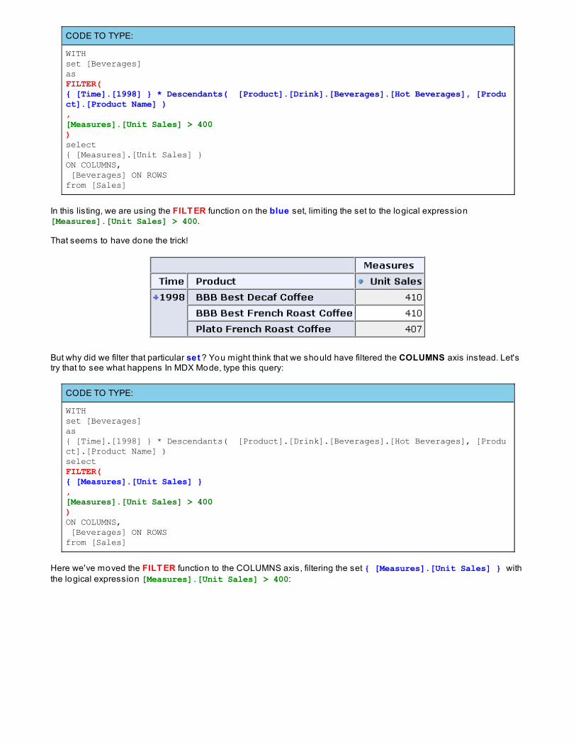
In this listing, we are using the FILT ER function on the blue set, limiting the set to the logical expression[Measures].[Unit Sales] > 400.
That seems to have done the trick!
But why did we filter that particular set ? You might think that we should have filtered the COLUMNS axis instead. Let'stry that to see what happens In MDX Mode, type this query:
CODE TO TYPE:
WITHset [Beverages]as{ [Time].[1998] } * Descendants( [Product].[Drink].[Beverages].[Hot Beverages], [Product].[Product Name] )selectFILTER({ [Measures].[Unit Sales] } ,[Measures].[Unit Sales] > 400)ON COLUMNS, [Beverages] ON ROWSfrom [Sales]
Here we've moved the FILT ER function to the COLUMNS axis, filtering the set { [Measures].[Unit Sales] } withthe logical expression [Measures].[Unit Sales] > 400:
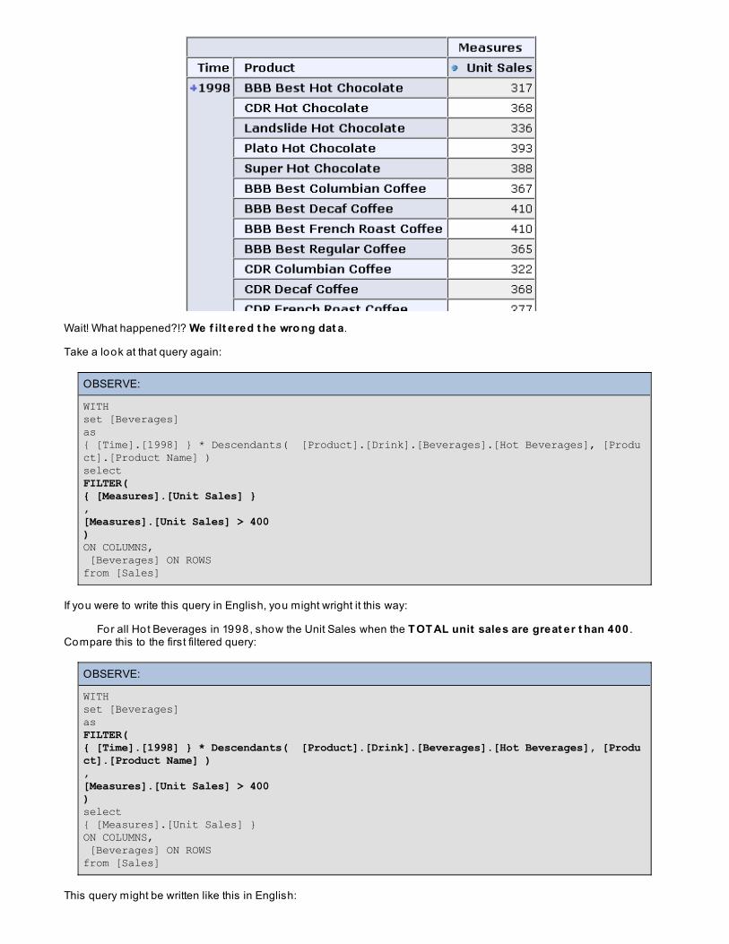
Wait! What happened?!? We f ilt ered t he wro ng dat a.
Take a look at that query again:
OBSERVE:
WITHset [Beverages]as{ [Time].[1998] } * Descendants( [Product].[Drink].[Beverages].[Hot Beverages], [Product].[Product Name] )selectFILTER({ [Measures].[Unit Sales] },[Measures].[Unit Sales] > 400)ON COLUMNS, [Beverages] ON ROWSfrom [Sales]
If you were to write this query in English, you might wright it this way:
For all Hot Beverages in 1998, show the Unit Sales when the T OT AL unit sales are great er t han 400 .Compare this to the first filtered query:
OBSERVE:
WITHset [Beverages]asFILTER({ [Time].[1998] } * Descendants( [Product].[Drink].[Beverages].[Hot Beverages], [Product].[Product Name] ),[Measures].[Unit Sales] > 400)select{ [Measures].[Unit Sales] }ON COLUMNS, [Beverages] ON ROWSfrom [Sales]
This query might be written like this in English:
For Ho t Beverages in 1998 wit h unit sales great er t han 400 , show the Unit Sales.
Notice the difference? The first query shows the Hot Beverages in 1998 where the t o t al sales fo r 1998 is greater than400, whereas the second query shows only Hot Beverages in 1998 that have sales greater than 400.
The difference is subtle, but important. When you filter data, you need to be careful and understand exactly what you areasking.
So, what else can we do with filtering?
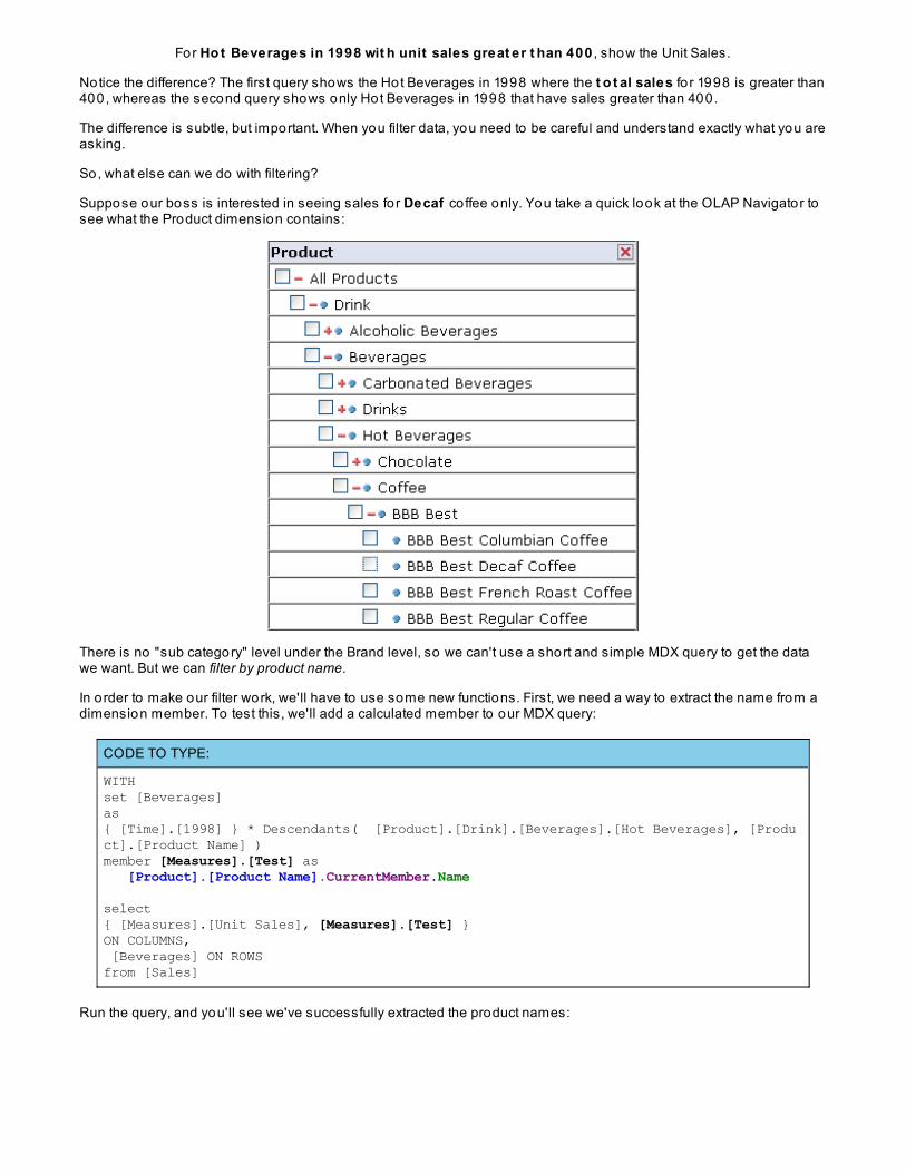
Suppose our boss is interested in seeing sales for Decaf co ffee only. You take a quick look at the OLAP Navigator tosee what the Product dimension contains:
There is no "sub category" level under the Brand level, so we can't use a short and simple MDX query to get the datawe want. But we can filter by product name.
In order to make our filter work, we'll have to use some new functions. First, we need a way to extract the name from adimension member. To test this, we'll add a calculated member to our MDX query:
CODE TO TYPE:
WITHset [Beverages]as{ [Time].[1998] } * Descendants( [Product].[Drink].[Beverages].[Hot Beverages], [Product].[Product Name] )member [Measures].[Test] as [Product].[Product Name].CurrentMember.Name
select{ [Measures].[Unit Sales], [Measures].[Test] }ON COLUMNS, [Beverages] ON ROWSfrom [Sales]
Run the query, and you'll see we've successfully extracted the product names:
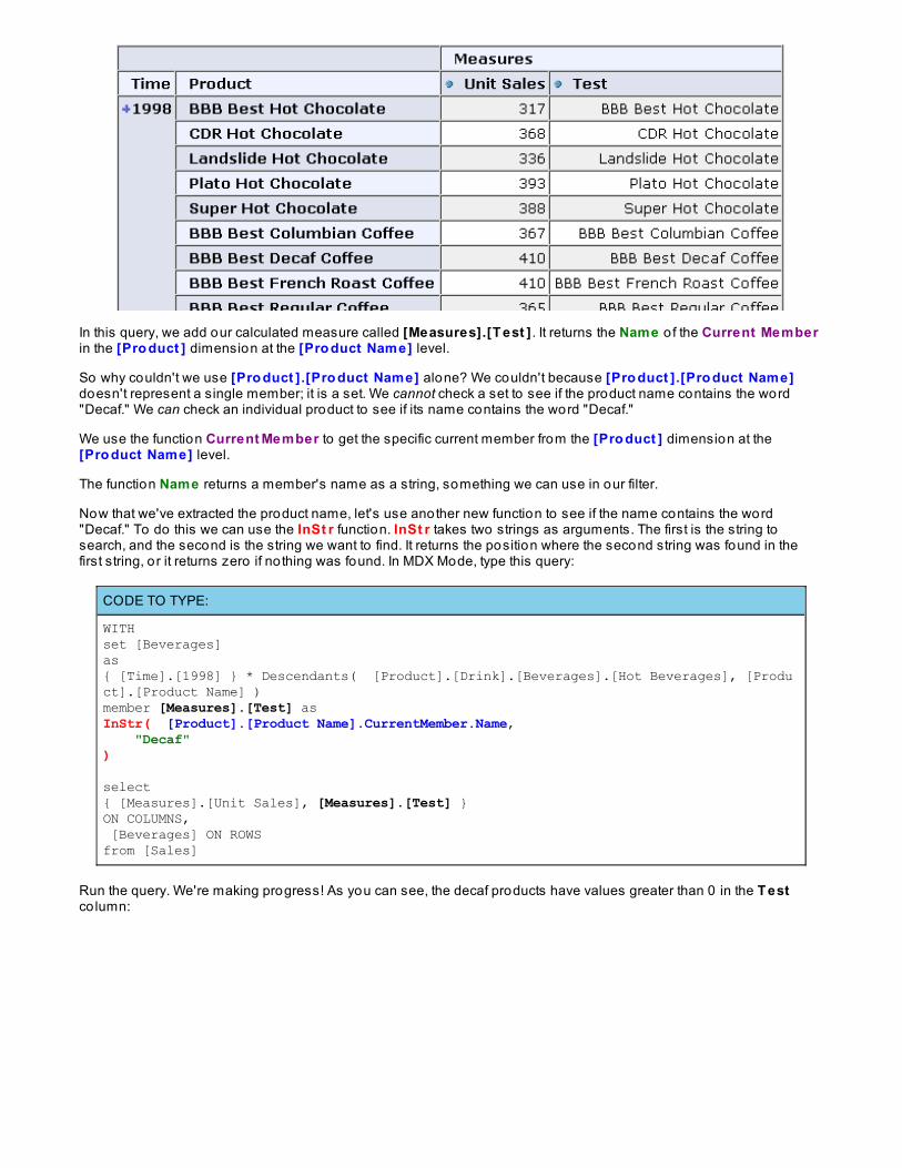
In this query, we add our calculated measure called [Measures].[T est ] . It returns the Name o f the Current Memberin the [Pro duct ] dimension at the [Pro duct Name] level.
So why couldn't we use [Pro duct ].[Pro duct Name] alone? We couldn't because [Pro duct ].[Pro duct Name]doesn't represent a single member; it is a set. We cannot check a set to see if the product name contains the word"Decaf." We can check an individual product to see if its name contains the word "Decaf."
We use the function Current Member to get the specific current member from the [Pro duct ] dimension at the[Pro duct Name] level.
The function Name returns a member's name as a string, something we can use in our filter.
Now that we've extracted the product name, let's use another new function to see if the name contains the word"Decaf." To do this we can use the InSt r function. InSt r takes two strings as arguments. The first is the string tosearch, and the second is the string we want to find. It returns the position where the second string was found in thefirst string, or it returns zero if no thing was found. In MDX Mode, type this query:
CODE TO TYPE:
WITHset [Beverages]as{ [Time].[1998] } * Descendants( [Product].[Drink].[Beverages].[Hot Beverages], [Product].[Product Name] )member [Measures].[Test] as InStr( [Product].[Product Name].CurrentMember.Name, "Decaf")
select{ [Measures].[Unit Sales], [Measures].[Test] }ON COLUMNS, [Beverages] ON ROWSfrom [Sales]
Run the query. We're making progress! As you can see, the decaf products have values greater than 0 in the T estco lumn:
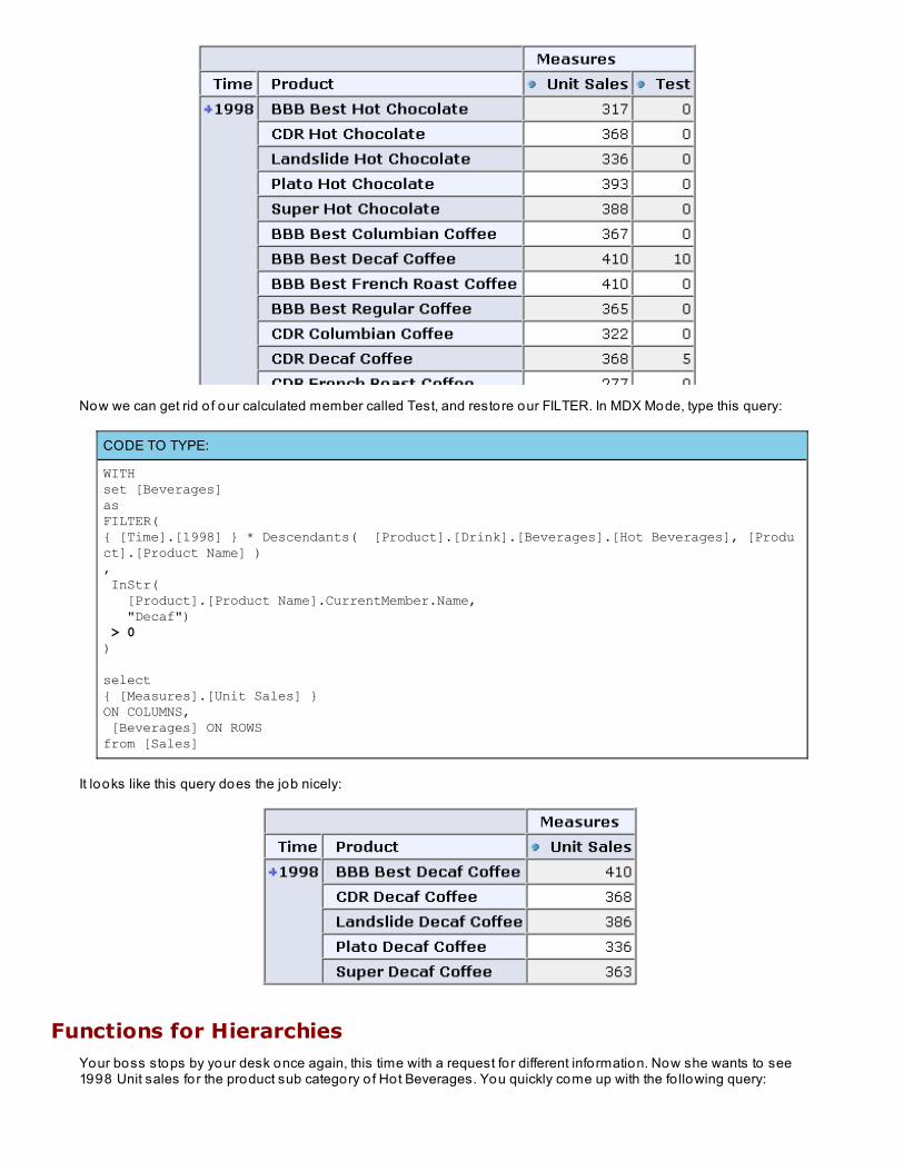
Now we can get rid o f our calculated member called Test, and restore our FILTER. In MDX Mode, type this query:
CODE TO TYPE:
WITHset [Beverages]asFILTER({ [Time].[1998] } * Descendants( [Product].[Drink].[Beverages].[Hot Beverages], [Product].[Product Name] ), InStr( [Product].[Product Name].CurrentMember.Name, "Decaf") > 0)
select{ [Measures].[Unit Sales] }ON COLUMNS, [Beverages] ON ROWSfrom [Sales]
It looks like this query does the job nicely:
Functions for HierarchiesYour boss stops by your desk once again, this time with a request fo r different information. Now she wants to see1998 Unit sales for the product sub category o f Hot Beverages. You quickly come up with the fo llowing query:
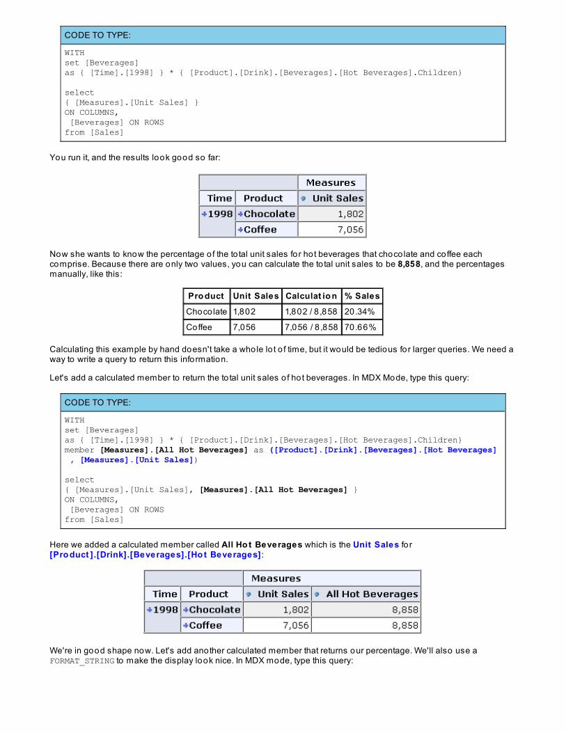
CODE TO TYPE:
WITHset [Beverages]as { [Time].[1998] } * { [Product].[Drink].[Beverages].[Hot Beverages].Children}
select{ [Measures].[Unit Sales] }ON COLUMNS, [Beverages] ON ROWSfrom [Sales]
You run it, and the results look good so far:
Now she wants to know the percentage o f the to tal unit sales for hot beverages that choco late and coffee eachcomprise. Because there are only two values, you can calculate the to tal unit sales to be 8,858, and the percentagesmanually, like this:
Pro duct Unit Sales Calculat io n % Sales
Chocolate 1,802 1,802 / 8 ,858 20.34%
Coffee 7,056 7,056 / 8 ,858 70.66%
Calculating this example by hand doesn't take a whole lo t o f time, but it would be tedious for larger queries. We need away to write a query to return this information.
Let's add a calculated member to return the to tal unit sales o f hot beverages. In MDX Mode, type this query:
CODE TO TYPE:
WITHset [Beverages]as { [Time].[1998] } * { [Product].[Drink].[Beverages].[Hot Beverages].Children}member [Measures].[All Hot Beverages] as ([Product].[Drink].[Beverages].[Hot Beverages] , [Measures].[Unit Sales])
select{ [Measures].[Unit Sales], [Measures].[All Hot Beverages] }ON COLUMNS, [Beverages] ON ROWSfrom [Sales]
Here we added a calculated member called All Ho t Beverages which is the Unit Sales fo r[Pro duct ].[Drink].[Beverages].[Ho t Beverages] :
We're in good shape now. Let's add another calculated member that returns our percentage. We'll also use aFORMAT_STRING to make the display look nice. In MDX mode, type this query:
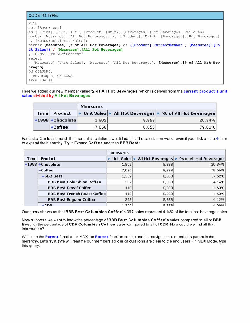
CODE TO TYPE:
WITHset [Beverages]as { [Time].[1998] } * { [Product].[Drink].[Beverages].[Hot Beverages].Children}member [Measures].[All Hot Beverages] as ([Product].[Drink].[Beverages].[Hot Beverages] , [Measures].[Unit Sales])member [Measures].[% of All Hot Beverages] as ([Product].CurrentMember , [Measures].[Unit Sales]) / [Measures].[All Hot Beverages], FORMAT_STRING="Percent"select{ [Measures].[Unit Sales], [Measures].[All Hot Beverages], [Measures].[% of All Hot Beverages] }ON COLUMNS, [Beverages] ON ROWSfrom [Sales]
Here we added our new member called % o f All Ho t Beverages, which is derived from the current pro duct 's unitsales divided by All Ho t Beverages:
Fantastic! Our to tals match the manual calculations we did earlier. The calculation works even if you click on the iconto expand the hierarchy. Try it. Expand Co f f ee and then BBB Best :
Our query shows us that BBB Best Co lumbian Co f f ee 's 367 sales represent 4.14% of the to tal hot beverage sales.
Now suppose we want to know the percentage o f BBB Best Co lumbian Co f f ee 's sales compared to all o f BBBBest , o r the percentage o f CDR Co lumbian Co f f ee sales compared to all o f CDR. How could we find all thatinformation?
We'll use the Parent function. In MDX the Parent function can be used to navigate to a member's parent in thehierarchy. Let's try it. (We will rename our members so our calculations are clear to the end users.) In MDX Mode, typethis query:
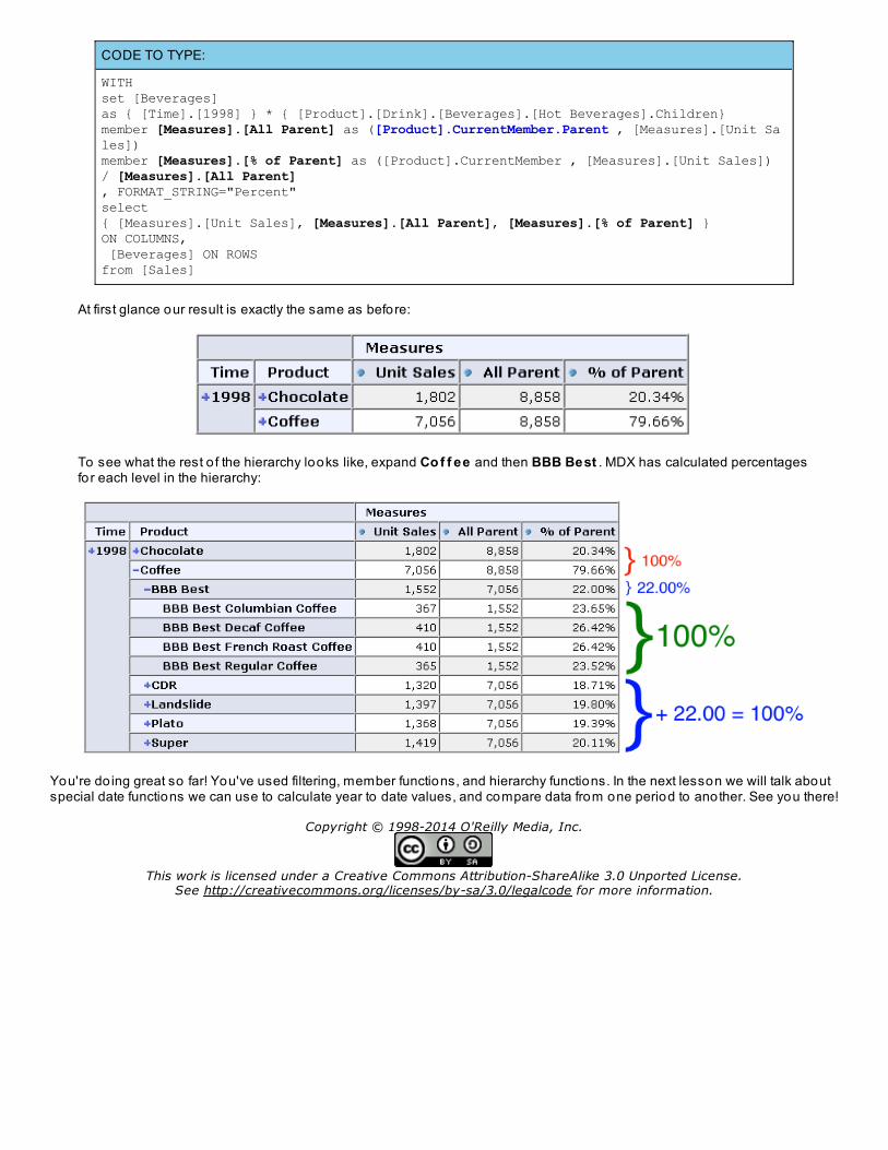
CODE TO TYPE:
WITHset [Beverages]as { [Time].[1998] } * { [Product].[Drink].[Beverages].[Hot Beverages].Children}member [Measures].[All Parent] as ([Product].CurrentMember.Parent , [Measures].[Unit Sales])member [Measures].[% of Parent] as ([Product].CurrentMember , [Measures].[Unit Sales]) / [Measures].[All Parent], FORMAT_STRING="Percent"select{ [Measures].[Unit Sales], [Measures].[All Parent], [Measures].[% of Parent] }ON COLUMNS, [Beverages] ON ROWSfrom [Sales]
At first glance our result is exactly the same as before:
To see what the rest o f the hierarchy looks like, expand Co f f ee and then BBB Best . MDX has calculated percentagesfor each level in the hierarchy:
You're do ing great so far! You've used filtering, member functions, and hierarchy functions. In the next lesson we will talk aboutspecial date functions we can use to calculate year to date values, and compare data from one period to another. See you there!
Copyright © 1998-2014 O'Reilly Media, Inc.
This work is licensed under a Creative Commons Attribution-ShareAlike 3.0 Unported License.See http://creativecommons.org/licenses/by-sa/3.0/legalcode for more information.
Traveling in Time
Welcome back! In the last lesson we learned to filter and to create percentages. In this lesson we'll look at functions that havebeen created to work with the date dimension.
Common Date Questions
Year to Date
A common question asked in the business world is "Ho w are we do ing so f ar?" There are several ways toanswer that question. You could calculate how many things you've so ld so far, o r compare this year's salesto last year's. Or maybe your company's status changes very quickly, so right now you are interested incomparing only this week's sales to last week's. However you approach the question, you'll need to use thedate dimension. Fortunately, MDX has an entire set o f functions specifically fo r the date dimension.
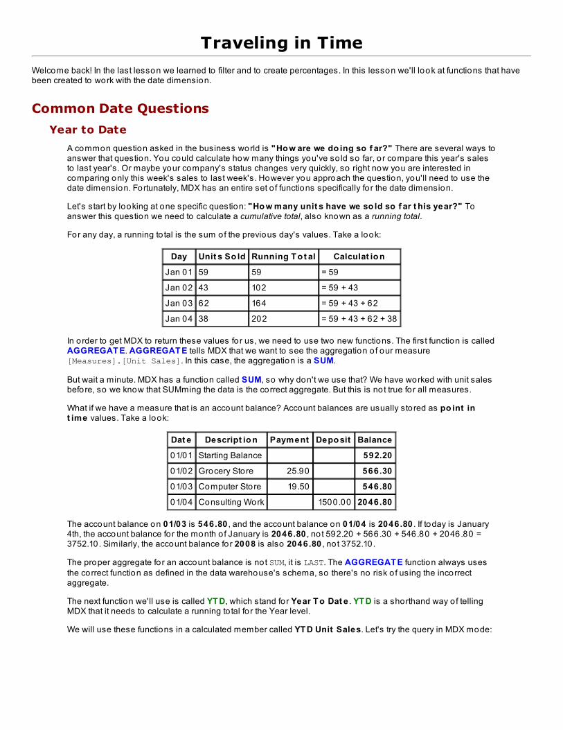
Let's start by looking at one specific question: "Ho w many unit s have we so ld so f ar t his year?" Toanswer this question we need to calculate a cumulative total, also known as a running total.
For any day, a running to tal is the sum of the previous day's values. Take a look:
Day Unit s So ld Running T o t al Calculat io n
Jan 01 59 59 = 59
Jan 02 43 102 = 59 + 43
Jan 03 62 164 = 59 + 43 + 62
Jan 04 38 202 = 59 + 43 + 62 + 38
In order to get MDX to return these values for us, we need to use two new functions. The first function is calledAGGREGAT E. AGGREGAT E tells MDX that we want to see the aggregation o f our measure[Measures].[Unit Sales]. In this case, the aggregation is a SUM.
But wait a minute. MDX has a function called SUM, so why don't we use that? We have worked with unit salesbefore, so we know that SUMming the data is the correct aggregate. But this is not true for all measures.
What if we have a measure that is an account balance? Account balances are usually stored as po int int ime values. Take a look:
Dat e Descript io n Payment Depo sit Balance
01/01 Starting Balance 592.20
01/02 Grocery Store 25.90 566.30
01/03 Computer Store 19.50 546.80
01/04 Consulting Work 1500.00 2046.80
The account balance on 01/03 is 546.80 , and the account balance on 01/04 is 2046.80 . If today is January4th, the account balance for the month o f January is 2046.80 , no t 592.20 + 566.30 + 546.80 + 2046.80 =3752.10. Similarly, the account balance for 2008 is also 2046.80 , no t 3752.10.
The proper aggregate for an account balance is not SUM, it is LAST. The AGGREGAT E function always usesthe correct function as defined in the data warehouse's schema, so there's no risk o f using the incorrectaggregate.
The next function we'll use is called YT D, which stand for Year T o Dat e . YT D is a shorthand way o f tellingMDX that it needs to calculate a running to tal fo r the Year level.
We will use these functions in a calculated member called YT D Unit Sales. Let's try the query in MDX mode:
CODE TO TYPE:
WITH member [Measures].[YTD Unit Sales] as AGGREGATE ( YTD(), [Measures].[Unit Sales] )select{ [Measures].[YTD Unit Sales] } ON COLUMNS,{ [Time].[1997] } on ROWS from [Sales]
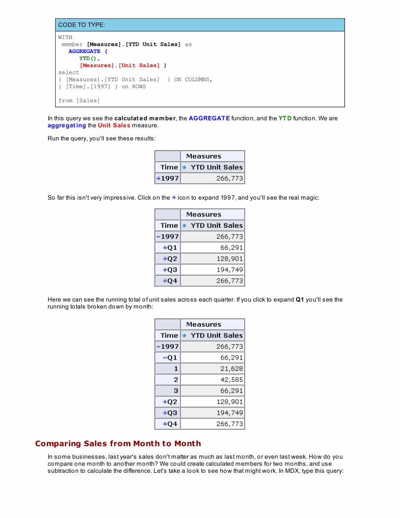
In this query we see the calculat ed member, the AGGREGAT E function, and the YT D function. We areaggregat ing the Unit Sales measure.
Run the query, you'll see these results:
So far this isn't very impressive. Click on the icon to expand 1997, and you'll see the real magic:
Here we can see the running to tal o f unit sales across each quarter. If you click to expand Q1 you'll see therunning to tals broken down by month:
Comparing Sales from Month to Month
In some businesses, last year's sales don't matter as much as last month, or even last week. How do youcompare one month to another month? We could create calculated members for two months, and usesubtraction to calculate the difference. Let's take a look to see how that might work. In MDX, type this query:

CODE TO TYPE:
WITH member [Measures].[Jan] as ( [Time].[1997].[Q1].[1], [Measures].[Unit Sales] ) member [Measures].[Feb] as ( [Time].[1997].[Q1].[2], [Measures].[Unit Sales] ) member [Measures].[Diff] as [Measures].[Feb] - [Measures].[Jan]select{ [Measures].[Jan], [Measures].[Feb], [Measures].[Diff] } ON COLUMNSfrom [Sales]
In this query we've created calculated members for January and February which are then used to calculatethe dif f erence in unit sales for those two months. Run the query, and you'll see the results:
everything looks good, but it would be great if we could just calculate the difference without having to specifyeach month. We can make short work o f this using a special MDX function called PrevMember.
The PrevMember function returns the previous member in a level. In o ther words, February's PrevMemberis January. Let's try it in our existing query to see how it works. In MDX, type this query:
CODE TO TYPE:
WITH member [Measures].[Jan] as ( [Time].[1997].[Q1].[2].PrevMember, [Measures].[Unit Sales] ) member [Measures].[Feb] as ( [Time].[1997].[Q1].[2], [Measures].[Unit Sales] ) member [Measures].[Diff] as [Measures].[Feb] - [Measures].[Jan]select{ [Measures].[Jan], [Measures].[Feb], [Measures].[Diff] } ON COLUMNSfrom [Sales]
Run the query and you'll see the same result as before:
PrevMember works with any dimension, not just date dimensions. Armed with this new function, let's rewriteour query so we can compare the current month to the prio r month. In MDX, type this query:
CODE TO TYPE:
WITH member [Measures].[Current Unit Sales] as ( [Time].CurrentMember, [Measures].[Unit Sales] ) member [Measures].[Prior Unit Sales] as ( [Time].CurrentMember.PrevMember, [Measures].[Unit Sales] ) member [Measures].[Diff] as [Measures].[Current Unit Sales] - [Measures].[Prior Unit Sales]select{ [Measures].[Current Unit Sales], [Measures].[Prior Unit Sales], [Measures].[Diff] } ON COLUMNS,{ [Time].[1997].[Q1].[1]:[Time].[1998].[Q4].[12] } on ROWSfrom [Sales]
In this query we've added a calculated member for the current mo nt h, and another calculated member forthe prio r mo nt h, using the PrevMember function. We calculate the dif f erence the same way as before.
Finally, we use the co lo n : to tell MDX that we want all months between January 1997 and December 1998
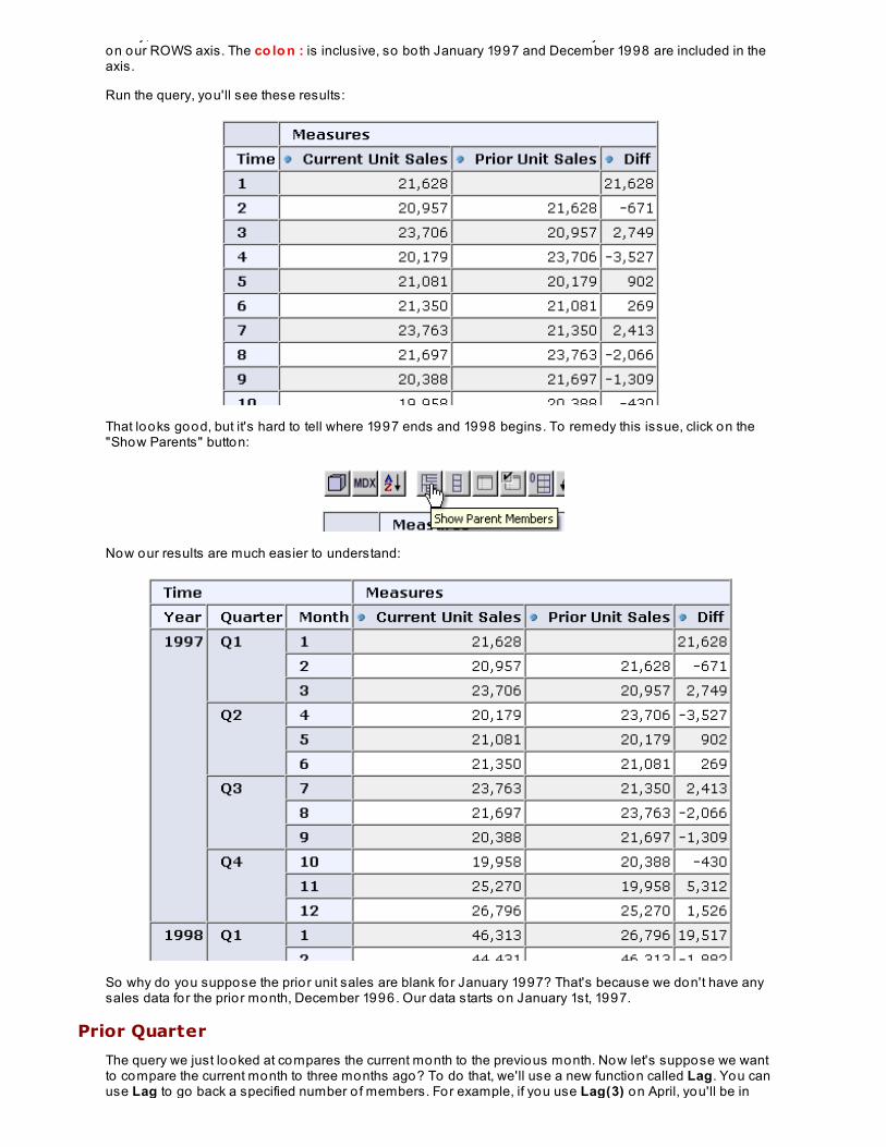
Finally, we use the co lo n : to tell MDX that we want all months between January 1997 and December 1998on our ROWS axis. The co lo n : is inclusive, so both January 1997 and December 1998 are included in theaxis.
Run the query, you'll see these results:
That looks good, but it's hard to tell where 1997 ends and 1998 begins. To remedy this issue, click on the"Show Parents" button:
Now our results are much easier to understand:
So why do you suppose the prio r unit sales are blank for January 1997? That's because we don't have anysales data for the prio r month, December 1996. Our data starts on January 1st, 1997.
Prior Quarter
The query we just looked at compares the current month to the previous month. Now let's suppose we wantto compare the current month to three months ago? To do that, we'll use a new function called Lag. You canuse Lag to go back a specified number o f members. For example, if you use Lag(3) on April, you'll be in

January. Lag(1) is exactly the same as PrevMember.
Let's try using Lag, replacing PrevMember with Lag(3) . In MDX, type this query:
CODE TO TYPE:
WITH member [Measures].[Current Unit Sales] as ( [Time].CurrentMember, [Measures].[Unit Sales] ) member [Measures].[Prior Unit Sales] as ( [Time].CurrentMember.Lag(3), [Measures].[Unit Sales] ) member [Measures].[Diff] as [Measures].[Current Unit Sales] - [Measures].[Prior Unit Sales]select{ [Measures].[Current Unit Sales], [Measures].[Prior Unit Sales], [Measures].[Diff] } ON COLUMNS,{ [Time].[1997].[Q1].[1]:[Time].[1998].[Q4].[12] } on ROWSfrom [Sales]
Run the query, and you'll see these results:
This looks great!
Parallel Periods
Suppose your manager wanted to compare 1998 sales to 1997 sales, but also wants the flexibility tocompare month to month, quarter to quarter, o r year to year. That seems like a tall o rder, doesn't it?
Lucky for you, MDX has a specific function to so lve this problem - Paralle lPerio d. If your current member isMarch 1998, Paralle lPerio d will take you back to March 1997. If your current member is Q2 1998,Paralle lPerio d will take you back to Q2 1997.
Let's try it! In MDX, type this query:
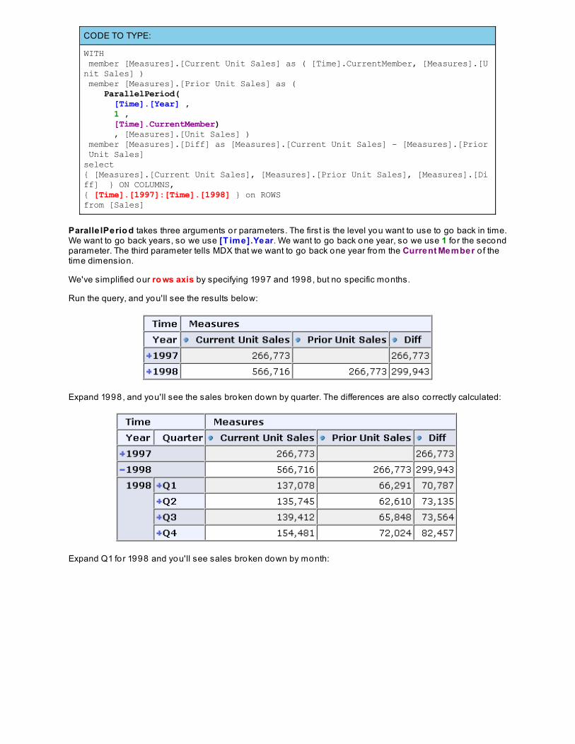
CODE TO TYPE:
WITH member [Measures].[Current Unit Sales] as ( [Time].CurrentMember, [Measures].[Unit Sales] ) member [Measures].[Prior Unit Sales] as ( ParallelPeriod( [Time].[Year] , 1 , [Time].CurrentMember) , [Measures].[Unit Sales] ) member [Measures].[Diff] as [Measures].[Current Unit Sales] - [Measures].[Prior Unit Sales]select{ [Measures].[Current Unit Sales], [Measures].[Prior Unit Sales], [Measures].[Diff] } ON COLUMNS,{ [Time].[1997]:[Time].[1998] } on ROWSfrom [Sales]
Paralle lPerio d takes three arguments or parameters. The first is the level you want to use to go back in time.We want to go back years, so we use [T ime].Year. We want to go back one year, so we use 1 fo r the secondparameter. The third parameter tells MDX that we want to go back one year from the Current Member o f thetime dimension.
We've simplified our ro ws axis by specifying 1997 and 1998, but no specific months.
Run the query, and you'll see the results below:
Expand 1998, and you'll see the sales broken down by quarter. The differences are also correctly calculated:
Expand Q1 for 1998 and you'll see sales broken down by month:
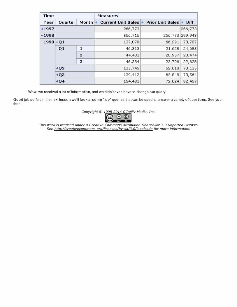
Wow, we received a lo t o f information, and we didn't even have to change our query!
Good job so far. In the next lesson we'll look at some "top" queries that can be used to answer a variety o f questions. See youthen!
Copyright © 1998-2014 O'Reilly Media, Inc.
This work is licensed under a Creative Commons Attribution-ShareAlike 3.0 Unported License.See http://creativecommons.org/licenses/by-sa/3.0/legalcode for more information.
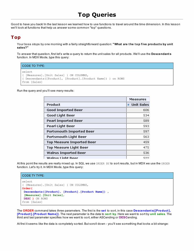
Top Queries
Good to have you back! In the last lesson we learned how to use functions to travel around the time dimension. In this lessonwe'll look at functions that help us answer some common "top" questions.
TopYour boss stops by one morning with a fairly straightforward question: "What are t he t o p f ive pro duct s by unitsales?"
To answer that question, first let's write a query to return the unit sales for all products. We'll use the Descendant sfunction. In MDX Mode, type this query:
CODE TO TYPE:
select{ [Measures].[Unit Sales] } ON COLUMNS,{ Descendants([Product], [Product].[Product Name]) } on ROWSfrom [Sales]
Run the query and you'll see many results:
At this po int the results are really mixed up. In SQL we use ORDER BY to sort results, but in MDX we use the ORDERfunction. Let's try it. In MDX Mode, type this query:
CODE TY TYPE:
select{ [Measures].[Unit Sales] } ON COLUMNS,Order( Descendants([Product], [Product].[Product Name]) , [Measures].[Unit Sales], DESC ) ON ROWSfrom [Sales]
The ORDER command takes three parameters. The first is the set to sort, in this case Descendant s([Pro duct ],[Pro duct ].[Pro duct Name]) . The next parameter is the data to so rt by. Here we want to sort by unit sales. Thethird and last parameter specifies how we want to sort, either ASCending or DESCending.
At first it seems like the data is completely sorted. But scro ll down - you'll see something that looks a bit strange:
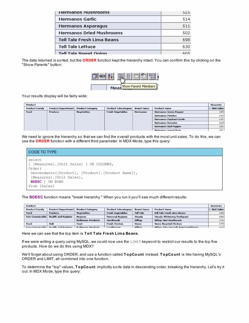
The data returned is sorted, but the ORDER function kept the hierarchy intact. You can confirm this by clicking on the"Show Parents" button:
Your results display will be fairly wide:
We need to ignore the hierarchy so that we can find the overall products with the most unit sales. To do this, we canuse the ORDER function with a different third parameter. In MDX Mode, type this query:
CODE TO TYPE:
select{ [Measures].[Unit Sales] } ON COLUMNS,Order( Descendants([Product], [Product].[Product Name]), [Measures].[Unit Sales], BDESC ) ON ROWSfrom [Sales]
The BDESC function means "break hierarchy." When you run it you'll see much different results:
Here we can see that the top item is T ell T ale Fresh Lima Beans.
If we were writing a query using MySQL, we could now use the LIMIT keyword to restrict our results to the top fiveproducts. How do we do this using MDX?
We'll fo rget about using ORDER, and use a function called T o pCo unt instead. T o pCo unt is like having MySQL'sORDER and LIMIT, all combined into one function.
To determine the "top" values, T o pCo unt implicitly sorts data in descending order, breaking the hierarchy. Let's try itout. In MDX Mode, type this query:

CODE TO TYPE:
select{ [Measures].[Unit Sales] } ON COLUMNS,TopCount( Descendants([Product], [Product].[Product Name]), 5, [Measures].[Unit Sales] ) ON ROWSfrom [Sales]
T o pCo unt takes three parameters. The first is the set to sort, in this case Descendant s([Pro duct ],[Pro duct ].[Pro duct Name]) . The second is the number o f items you want to return, 5 . The third parameter is thedata used to determine the t o p values; fo r us this is the unit sales. And here we have our top five values:
We are looking good.
Now suppose your boss stops by your desk again, this time with a slightly different question: "What pro duct srepresent t he t o p 1% o f o ur unit sales?"
In order to answer this question, we need to know the to tal unit sales for all products, then sort the products by unitsales. The subset o f products whose combined unit sales is at least 1% of the to tal is returned.
Fortunately, MDX has a built in function to handle this work for us called T o pPercent . Let's try it. In MDX Mode, typethis query:
CODE TO TYPE:
select{ [Measures].[Unit Sales] } ON COLUMNS,TopPercent( Descendants([Product], [Product].[Product Name]), 1, [Measures].[Unit Sales] ) ON ROWSfrom [Sales]
We are using the T o pPercent function on the same set -- Descendant s([Pro duct ], [Pro duct ].[Pro duct Name])-- but this time we want the top 1% o f [Measures].[Unit Sales] .
Run the query. You'll see the fo llowing results:
This is much easier than returning the same data with SQL!
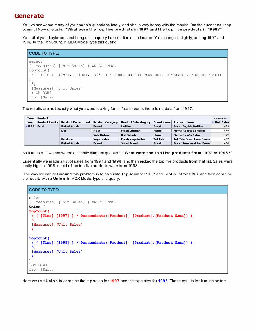
GenerateYou've answered many o f your boss's questions lately, and she is very happy with the results. But the questions keepcoming! Now she asks, "What were t he t o p f ive pro duct s in 1997 and t he t o p f ive pro duct s in 1998?"
You sit at your keyboard, and bring up the query from earlier in the lesson. You change it slightly, adding 1997 and1998 to the TopCount. In MDX Mode, type this query:
CODE TO TYPE:
select{ [Measures].[Unit Sales] } ON COLUMNS,TopCount( ( { [Time].[1997], [Time].[1998] } * Descendants([Product], [Product].[Product Name]) ), 5, [Measures].[Unit Sales] ) ON ROWSfrom [Sales]
The results are not exactly what you were looking for. In fact it seems there is no data from 1997:
As it turns out, we answered a slightly different question: "What were t he t o p f ive pro duct s f ro m 1997 or 1998?"
Essentially we made a list o f sales from 1997 and 1998, and then picked the top five products from that list. Sales werereally high in 1998, so all o f the top five products were from 1998.
One way we can get around this problem is to calculate TopCount fo r 1997 and TopCount fo r 1998, and then combinethe results with a Unio n. In MDX Mode, type this query:
CODE TO TYPE:
select{ [Measures].[Unit Sales] } ON COLUMNS,Union (TopCount( ( { [Time].[1997] } * Descendants([Product], [Product].[Product Name]) ), 5, [Measures].[Unit Sales] ), TopCount( ( { [Time].[1998] } * Descendants([Product], [Product].[Product Name]) ), 5, [Measures].[Unit Sales] )) ON ROWSfrom [Sales]
Here we use Unio n to combine the top sales for 1997 and the top sales for 1998. These results look much better:

The last MDX query certainly worked, but it required quite a bit o f repetitive typing. If our manager wanted us to return thetop 20 products for a period o f 5 years, we would have a lo t o f work to do. There must be a better way. Of course thereis. MDX has a function called Generat e that can make life much easier.
Generat e takes two sets as parameters. Tuples in the second set are applied to each tuple in the first set, and theresults are unioned and returned. In o ther words, Generat e does exactly what we just did, but without all that typing.
Let's take a look. In MDX Mode, type this query:
CODE TO TYPE:
select{ [Measures].[Unit Sales] } ON COLUMNS,Generate ({ [Time].[1997], [Time].[1998] } , TopCount( ( { [Time].CurrentMember } * Descendants([Product], [Product].[Product Name]) ), 5, [Measures].[Unit Sales] ) ) ON ROWSfrom [Sales]
The first parameter to Generat e is our set o f tuples from the t ime dimension. The second parameter is ourTopCount function - but this time we use T ime.Current Member instead o f actually specifying a member from thetime dimension.
When this MDX query runs, the TopCount fo r 1997 is calculated, then the TopCount fo r 1998 is calculated. The resultsare unioned and returned:
Generat e saved us a lo t o f work!
We learned a lo t in this lesson. In the next lesson we'll learn one last MDX function that will help us predict the future. Stay tuned!
Copyright © 1998-2014 O'Reilly Media, Inc.
This work is licensed under a Creative Commons Attribution-ShareAlike 3.0 Unported License.See http://creativecommons.org/licenses/by-sa/3.0/legalcode for more information.

Predicting the Future
How to Predict the FuturePeople have been trying to predict the future for a long time. We want to know what the weather will be like tomorrow, ifour stock will go up in value, or what our sales will be next month. When most people try to predict the future, they areusually refer to historical data as guide for future activity. So how does it work for us as database administrators?
Let's use an example. Suppose you set up a lemonade stand. You carefully record your sales during your first week:
Day Cups So ld
1 5
2 10
3 15
4 20
5 25
6 30
7 35
Your business is really growing! If this trend continues, you could probably expect to sell 40 cups o f lemonade onyour eighth day in business. You can make this prediction because on each day you so ld five more cups than the daybefore.
In the real world sales are rarely this nice and orderly. In fact, real world sales might look something like this:
Day Cups So ld
1 2
2 6
3 5
4 11
5 9
6 15
7 16
We can graph this data, and come up with this chart:
Using our ruler, we can attempt to draw a nice line through our graph to show how our sales are increasing:
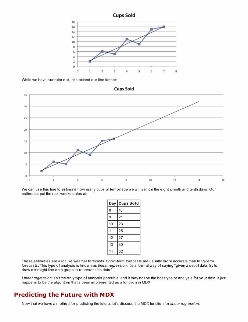
While we have our ruler out, let's extend our line farther:
We can use this line to estimate how many cups o f lemonade we will sell on the eighth, ninth and tenth days. Ourestimates put the next weeks sales at:
Day Cups So ld
8 18
9 21
10 23
11 25
12 27
13 30
14 32
These estimates are a lo t like weather fo recasts. Short-term forecasts are usually more accurate than long-termforecasts. This type o f analysis is known as linear regression. It's a fo rmal way o f saying "given a set o f data, try todraw a straight line on a graph to represent the data."
Linear regression isn't the only type o f analysis possible, and it may not be the best type o f analysis fo r your data. It justhappens to be the algorithm that's been implemented as a function in MDX.
Predicting the Future with MDXNow that we have a method for predicting the future, let's discuss the MDX function for linear regression.
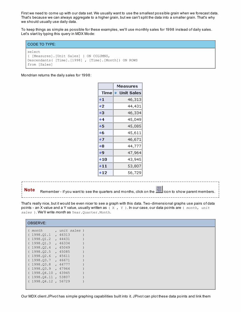
First we need to come up with our data set. We usually want to use the smallest possible grain when we forecast data.That's because we can always aggregate to a higher grain, but we can't split the data into a smaller grain. That's whywe should usually use daily data.
To keep things as simple as possible for these examples, we'll use monthly sales for 1998 instead o f daily sales.Let's start by typing this query in MDX Mode:
CODE TO TYPE:
select{ [Measures].[Unit Sales] } ON COLUMNS,Descendants( [Time].[1998] , [Time].[Month]) ON ROWSfrom [Sales]
Mondrian returns the daily sales for 1998:
Note Remember - if you want to see the quarters and months, click on the icon to show parent members.
That's really nice, but it would be even nicer to see a graph with this data. Two-dimensional graphs use pairs o f datapo ints - an X value and a Y value, usually written as ( X , Y ). In our case, our data po ints are ( month, unitsales ). We'll write month as Year.Quarter.Month.
OBSERVE:
( month , unit sales )( 1998.Q1.1 , 46313 )( 1998.Q1.2 , 44431 )( 1998.Q1.3 , 46334 )( 1998.Q2.4 , 45049 )( 1998.Q2.5 , 45085 )( 1998.Q2.6 , 45611 )( 1998.Q3.7 , 46671 )( 1998.Q3.8 , 44777 )( 1998.Q3.9 , 47964 )( 1998.Q4.10 , 43945 )( 1998.Q4.11 , 53807 )( 1998.Q4.12 , 56729 )
Our MDX client JPivot has simple graphing capabilities built into it. JPivot can plo t these data po ints and link them
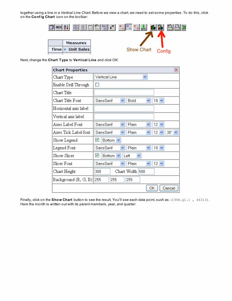
together using a line in a Vertical Line Chart. Before we view a chart, we need to set some properties. To do this, clickon the Co nf ig Chart icon on the too lbar:
Next, change the Chart T ype to Vert ical Line and click OK:
Finally, click on the Sho w Chart button to see the result. You'll see each data po int, such as (1998.Q1.1 , 46313).Here the month is written out with its parent members, year, and quarter:
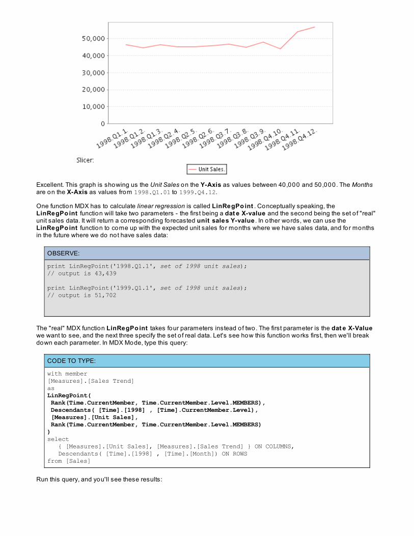
Excellent. This graph is showing us the Unit Sales on the Y-Axis as values between 40,000 and 50,000. The Monthsare on the X-Axis as values from 1998.Q1.01 to 1999.Q4.12.
One function MDX has to calculate linear regression is called LinRegPo int . Conceptually speaking, theLinRegPo int function will take two parameters - the first being a dat e X-value and the second being the set o f "real"unit sales data. It will return a corresponding forecasted unit sales Y-value . In o ther words, we can use theLinRegPo int function to come up with the expected unit sales for months where we have sales data, and for monthsin the future where we do not have sales data:
OBSERVE:
print LinRegPoint('1998.Q1.1', set of 1998 unit sales);// output is 43,439
print LinRegPoint('1999.Q1.1', set of 1998 unit sales);// output is 51,702
The "real" MDX function LinRegPo int takes four parameters instead o f two. The first parameter is the dat e X-Valuewe want to see, and the next three specify the set o f real data. Let's see how this function works first, then we'll breakdown each parameter. In MDX Mode, type this query:
CODE TO TYPE:
with member[Measures].[Sales Trend]asLinRegPoint( Rank(Time.CurrentMember, Time.CurrentMember.Level.MEMBERS), Descendants( [Time].[1998] , [Time].CurrentMember.Level), [Measures].[Unit Sales], Rank(Time.CurrentMember, Time.CurrentMember.Level.MEMBERS))select { [Measures].[Unit Sales], [Measures].[Sales Trend] } ON COLUMNS, Descendants( [Time].[1998] , [Time].[Month]) ON ROWSfrom [Sales]
Run this query, and you'll see these results:
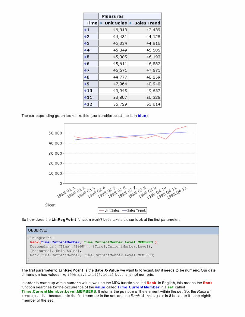
The corresponding graph looks like this (our trend/forecast line is in blue ):
So how does the LinRegPo int function work? Let's take a closer look at the first parameter:
OBSERVE:
LinRegPoint( Rank(Time.CurrentMember, Time.CurrentMember.Level.MEMBERS ), Descendants( [Time].[1998] , [Time].CurrentMember.Level), [Measures].[Unit Sales], Rank(Time.CurrentMember, Time.CurrentMember.Level.MEMBERS))
The first parameter to LinRegPo int is the dat e X-Value we want to fo recast, but it needs to be numeric. Our datedimension has values like 1998.Q1.1 to 1998.Q4.12, but this is not numeric.
In order to come up with a numeric value, we use the MDX function called Rank. In English, this means the Rankfunction searches for the occurrence o f the value called T ime.Current Member in a set calledT ime.Current Member.Level.MEMBERS . It returns the position o f the element within the set. So, the Rank o f1998.Q1.1 is 1 because it is the first member in the set, and the Rank o f 1998.Q3.8 is 8 because it is the eighthmember o f the set.
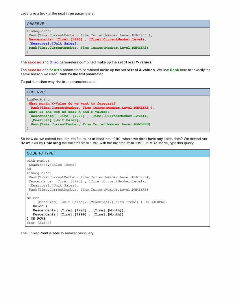
Let's take a look at the next three parameters:
OBSERVE:
LinRegPoint( Rank(Time.CurrentMember, Time.CurrentMember.Level.MEMBERS ), Descendants( [Time].[1998] , [Time].CurrentMember.Level), [Measures].[Unit Sales], Rank(Time.CurrentMember, Time.CurrentMember.Level.MEMBERS))
The seco nd and t hird parameters combined make up the set o f real Y-values.
The seco nd and f o urt h parameters combined make up the set o f real X-values. We use Rank here for exactly thesame reason we used Rank for the first parameter.
To put it another way, the four parameters are:
OBSERVE:
LinRegPoint( What month X-Value do we want to forecast? Rank(Time.CurrentMember, Time.CurrentMember.Level.MEMBERS ), What is the set of real X and Y Values? Descendants( [Time].[1998] , [Time].CurrentMember.Level), [Measures].[Unit Sales], Rank(Time.CurrentMember, Time.CurrentMember.Level.MEMBERS))
So how do we extend this into the future, or at least into 1999, where we don't have any sales data? We extend ourRo ws axis by Unio ning the months from 1998 with the months from 1999. In MDX Mode, type this query:
CODE TO TYPE:
with member[Measures].[Sales Trend]asLinRegPoint( Rank(Time.CurrentMember, Time.CurrentMember.Level.MEMBERS), Descendants( [Time].[1998] , [Time].CurrentMember.Level), [Measures].[Unit Sales], Rank(Time.CurrentMember, Time.CurrentMember.Level.MEMBERS))select { [Measures].[Unit Sales], [Measures].[Sales Trend] } ON COLUMNS, Union ( Descendants( [Time].[1998] , [Time].[Month]), Descendants( [Time].[1999] , [Time].[Month])) ON ROWSfrom [Sales]
The LinRegPoint is able to answer our query:
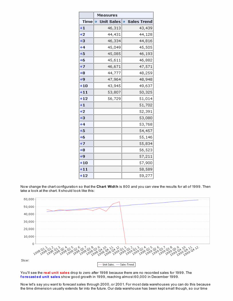
Now change the chart configuration so that the Chart Widt h is 800 and you can view the results fo r all o f 1999. Thentake a look at the chart. It should look like this:
You'll see the real unit sales drop to zero after 1998 because there are no recorded sales for 1999. Thef o recast ed unit sales show good growth in 1999, reaching almost 60,000 in December 1999.
Now let's say you want to fo recast sales through 2000, or 2001. For most data warehouses you can do this becausethe time dimension usually extends far into the future. Our data warehouse has been kept small though, so our time
dimension only has values from 1997 to 1999.
Linear regression is just one technique that we can use to forecast the future. Depending on your data, it may not be the mostaccurate method, but it can help you get close.
In the next lesson we'll switch gears and discuss the way Mondrian connects to the relational data warehouse through itsschema. Keep go ing, you're do ing great!
Copyright © 1998-2014 O'Reilly Media, Inc.
This work is licensed under a Creative Commons Attribution-ShareAlike 3.0 Unported License.See http://creativecommons.org/licenses/by-sa/3.0/legalcode for more information.
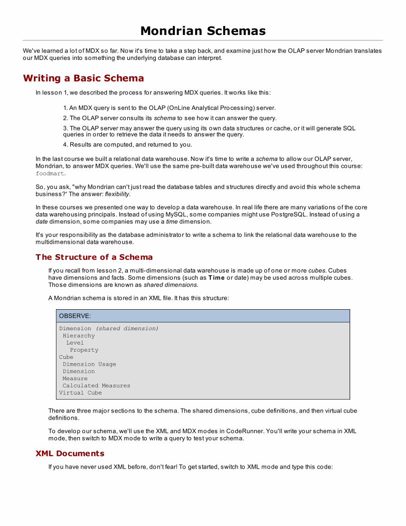
Mondrian Schemas
We've learned a lo t o f MDX so far. Now it's time to take a step back, and examine just how the OLAP server Mondrian translatesour MDX queries into something the underlying database can interpret.
Writing a Basic SchemaIn lesson 1, we described the process for answering MDX queries. It works like this:
1. An MDX query is sent to the OLAP (OnLine Analytical Processing) server.2. The OLAP server consults its schema to see how it can answer the query.3. The OLAP server may answer the query using its own data structures or cache, or it will generate SQLqueries in order to retrieve the data it needs to answer the query.4. Results are computed, and returned to you.
In the last course we built a relational data warehouse. Now it's time to write a schema to allow our OLAP server,Mondrian, to answer MDX queries. We'll use the same pre-built data warehouse we've used throughout this course:foodmart.
So, you ask, "why Mondrian can't just read the database tables and structures directly and avo id this whole schemabusiness?' The answer: flexibility.
In these courses we presented one way to develop a data warehouse. In real life there are many variations o f the coredata warehousing principals. Instead o f using MySQL, some companies might use PostgreSQL. Instead o f using adate dimension, some companies may use a time dimension.
It's your responsibility as the database administrator to write a schema to link the relational data warehouse to themultidimensional data warehouse.
The Structure of a Schema
If you recall from lesson 2, a multi-dimensional data warehouse is made up o f one or more cubes. Cubeshave dimensions and facts. Some dimensions (such as T ime o r date) may be used across multiple cubes.Those dimensions are known as shared dimensions.
A Mondrian schema is stored in an XML file. It has this structure:
OBSERVE:
Dimension (shared dimension) Hierarchy Level PropertyCube Dimension Usage Dimension Measure Calculated MeasuresVirtual Cube
There are three major sections to the schema. The shared dimensions, cube definitions, and then virtual cubedefinitions.
To develop our schema, we'll use the XML and MDX modes in CodeRunner. You'll write your schema in XMLmode, then switch to MDX mode to write a query to test your schema.
XML Documents
If you have never used XML before, don't fear! To get started, switch to XML mode and type this code:
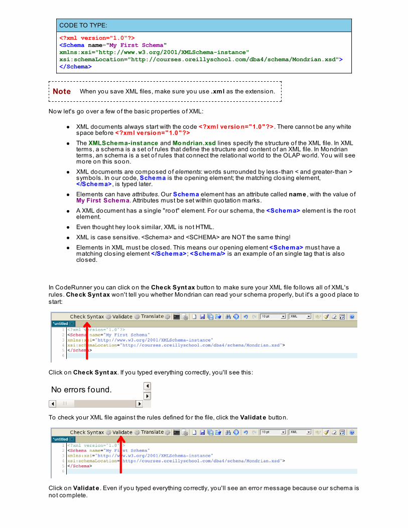
CODE TO TYPE:
<?xml version="1.0"?><Schema name="My First Schema"xmlns:xsi="http://www.w3.org/2001/XMLSchema-instance"xsi:schemaLocation="http://courses.oreillyschool.com/dba4/schema/Mondrian.xsd"></Schema>
Note When you save XML files, make sure you use .xml as the extension.
Now let's go over a few of the basic properties o f XML:
XML documents always start with the code <?xml versio n="1.0"?> . There cannot be any whitespace before <?xml versio n="1.0"?>The XMLSchema-inst ance and Mo ndrian.xsd lines specify the structure o f the XML file. In XMLterms, a schema is a set o f rules that define the structure and content o f an XML file. In Mondrianterms, an schema is a set o f rules that connect the relational world to the OLAP world. You will seemore on this soon.XML documents are composed o f elements: words surrounded by less-than < and greater-than >symbols. In our code, Schema is the opening element; the matching closing element,</Schema> , is typed later.Elements can have attributes. Our Schema element has an attribute called name , with the value o fMy First Schema. Attributes must be set within quotation marks.A XML document has a single "root" element. For our schema, the <Schema> element is the rootelement.Even thought hey look similar, XML is not HTML.XML is case sensitive. <Schema> and <SCHEMA> are NOT the same thing!Elements in XML must be closed. This means our opening element <Schema> must have amatching closing element </Schema> ; <Schema/> is an example o f an single tag that is alsoclosed.
In CodeRunner you can click on the Check Synt ax button to make sure your XML file fo llows all o f XML'srules. Check Synt ax won't tell you whether Mondrian can read your schema properly, but it's a good place tostart:
Click on Check Synt ax. If you typed everything correctly, you'll see this:
No errors found.
To check your XML file against the rules defined for the file, click the Validat e button.
Click on Validat e . Even if you typed everything correctly, you'll see an error message because our schema isnot complete.

Checking syntax and validating your document can help you track down problems with your schema, howeverit is still possible to have a syntactically correct and valid schema that gives an error when used withMondrian, as you will see.
Create a new document, set it to MDX mode and type this short query:
CODE TO TYPE:
select{ [Measures].[Unit Sales] } ON COLUMNSfrom [Sales]
When you're done, click on Run Query. Your XML Schema and your MDX query are sent to the Mondrianserver, which responds with this:
This error is the appropriate result, because we haven't defined any cubes in our schema. (We will shortly
though.) You can click on the button to see the documentation o f your schema. Since we don't haveanything defined right now, when we check our schema documentation, not much is returned:
There is another way we can preview our schema. Since the schema is an XML document, we can use XSL toconvert our XML document to an HTML document. Don't worry about the specifics o f this transformation.
Switch back to your XML file. Update it so it contains the fo llowing line:
CODE TO TYPE:
<?xml version="1.0"?><?xml-stylesheet href="http://courses.oreillyschool.com/dba4/schema/MetaData.xsl" type="text/xsl"?><Schema name="My First Schema"xmlns:xsi="http://www.w3.org/2001/XMLSchema-instance"xsi:schemaLocation="http://courses.oreillyschool.com/dba4/schema/Mondrian.xsd"></Schema>
Next, click the T ranslat e button:
Your schema is reformatted and displayed to you, just like before:
For more information on XML and XSL modes, check out the XML course.
Shared Dimensions
Our first task when authoring a schema is to define the shared dimensions. Let's get started!
The first shared dimension that we're go ing to create is the T ime dimension. The underlying table for T imeis called time_by_day. Back in lesson 2, we learned that all dimensions in MDX are hierarchical. Forexample, the time dimension has a hierarchy o f Year -> Quart er -> Mo nt h -> Day.
Let's log into the database to examine its structure.
NoteIn this course we will tell you which tables to use for facts and dimensions. If you were workingon your own data warehousing pro ject, you would consult the documentation for your datawarehouse.
Switch to Unix mode, then run this command to connect to the foodmart database:
CODE TO TYPE:
cold1:~$ mysql -h sql -u anonymous foodmart
You don't need to enter a password to connect to this database. If you typed everything correctly, you'll seethis:
OBSERVE:
cold1:~$ mysql -h sql -u anonymous foodmartReading table information for completion of table and column namesYou can turn off this feature to get a quicker startup with -A
Welcome to the MySQL monitor. Commands end with ; or \g.Your MySQL connection id is 442243Server version: 5.0.62-log Source distribution
Type 'help;' or '\h' for help. Type '\c' to clear the buffer.
mysql>
Now we can use the describe command to see what time_by_day looks like. At the MySQL prompt, type this:
CODE TO TYPE:
mysql> describe time_by_day;
This table isn't exceedingly large:
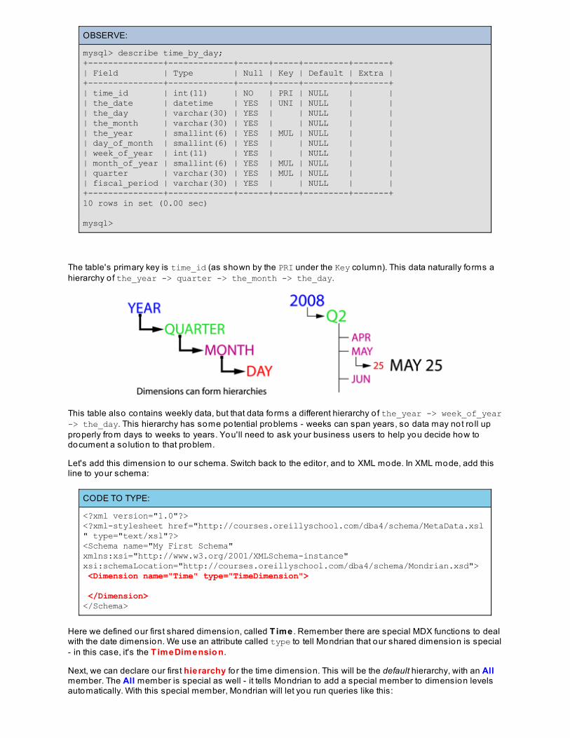
OBSERVE:
mysql> describe time_by_day;+---------------+-------------+------+-----+---------+-------+| Field | Type | Null | Key | Default | Extra |+---------------+-------------+------+-----+---------+-------+| time_id | int(11) | NO | PRI | NULL | | | the_date | datetime | YES | UNI | NULL | | | the_day | varchar(30) | YES | | NULL | | | the_month | varchar(30) | YES | | NULL | | | the_year | smallint(6) | YES | MUL | NULL | | | day_of_month | smallint(6) | YES | | NULL | | | week_of_year | int(11) | YES | | NULL | | | month_of_year | smallint(6) | YES | MUL | NULL | | | quarter | varchar(30) | YES | MUL | NULL | | | fiscal_period | varchar(30) | YES | | NULL | | +---------------+-------------+------+-----+---------+-------+10 rows in set (0.00 sec)
mysql>
The table's primary key is time_id (as shown by the PRI under the Key co lumn). This data naturally fo rms ahierarchy o f the_year -> quarter -> the_month -> the_day.
This table also contains weekly data, but that data forms a different hierarchy o f the_year -> week_of_year-> the_day. This hierarchy has some potential problems - weeks can span years, so data may not ro ll upproperly from days to weeks to years. You'll need to ask your business users to help you decide how todocument a so lution to that problem.
Let's add this dimension to our schema. Switch back to the editor, and to XML mode. In XML mode, add thisline to your schema:
CODE TO TYPE:
<?xml version="1.0"?> <?xml-stylesheet href="http://courses.oreillyschool.com/dba4/schema/MetaData.xsl" type="text/xsl"?><Schema name="My First Schema"xmlns:xsi="http://www.w3.org/2001/XMLSchema-instance"xsi:schemaLocation="http://courses.oreillyschool.com/dba4/schema/Mondrian.xsd"> <Dimension name="Time" type="TimeDimension"> </Dimension></Schema>
Here we defined our first shared dimension, called T ime . Remember there are special MDX functions to dealwith the date dimension. We use an attribute called type to tell Mondrian that our shared dimension is special- in this case, it's the T imeDimensio n.
Next, we can declare our first hierarchy fo r the time dimension. This will be the default hierarchy, with an Allmember. The All member is special as well - it tells Mondrian to add a special member to dimension levelsautomatically. With this special member, Mondrian will let you run queries like this:
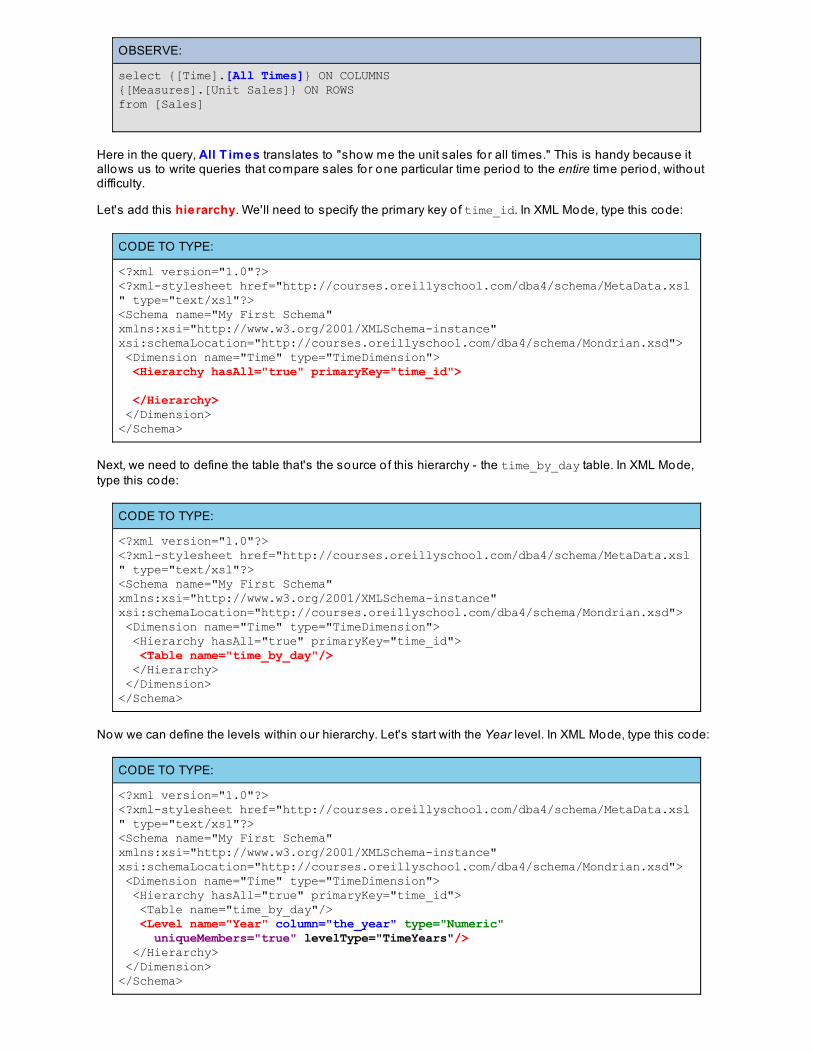
OBSERVE:
select {[Time].[All Times]} ON COLUMNS{[Measures].[Unit Sales]} ON ROWSfrom [Sales]
Here in the query, All T imes translates to "show me the unit sales for all times." This is handy because itallows us to write queries that compare sales for one particular time period to the entire time period, withoutdifficulty.
Let's add this hierarchy. We'll need to specify the primary key o f time_id. In XML Mode, type this code:
CODE TO TYPE:
<?xml version="1.0"?> <?xml-stylesheet href="http://courses.oreillyschool.com/dba4/schema/MetaData.xsl" type="text/xsl"?><Schema name="My First Schema"xmlns:xsi="http://www.w3.org/2001/XMLSchema-instance"xsi:schemaLocation="http://courses.oreillyschool.com/dba4/schema/Mondrian.xsd"> <Dimension name="Time" type="TimeDimension"> <Hierarchy hasAll="true" primaryKey="time_id"> </Hierarchy> </Dimension></Schema>
Next, we need to define the table that's the source o f this hierarchy - the time_by_day table. In XML Mode,type this code:
CODE TO TYPE:
<?xml version="1.0"?> <?xml-stylesheet href="http://courses.oreillyschool.com/dba4/schema/MetaData.xsl" type="text/xsl"?><Schema name="My First Schema"xmlns:xsi="http://www.w3.org/2001/XMLSchema-instance"xsi:schemaLocation="http://courses.oreillyschool.com/dba4/schema/Mondrian.xsd"> <Dimension name="Time" type="TimeDimension"> <Hierarchy hasAll="true" primaryKey="time_id"> <Table name="time_by_day"/> </Hierarchy> </Dimension></Schema>
Now we can define the levels within our hierarchy. Let's start with the Year level. In XML Mode, type this code:
CODE TO TYPE:
<?xml version="1.0"?><?xml-stylesheet href="http://courses.oreillyschool.com/dba4/schema/MetaData.xsl" type="text/xsl"?><Schema name="My First Schema"xmlns:xsi="http://www.w3.org/2001/XMLSchema-instance"xsi:schemaLocation="http://courses.oreillyschool.com/dba4/schema/Mondrian.xsd"> <Dimension name="Time" type="TimeDimension"> <Hierarchy hasAll="true" primaryKey="time_id"> <Table name="time_by_day"/> <Level name="Year" column="the_year" type="Numeric" uniqueMembers="true" levelType="TimeYears"/> </Hierarchy> </Dimension></Schema>
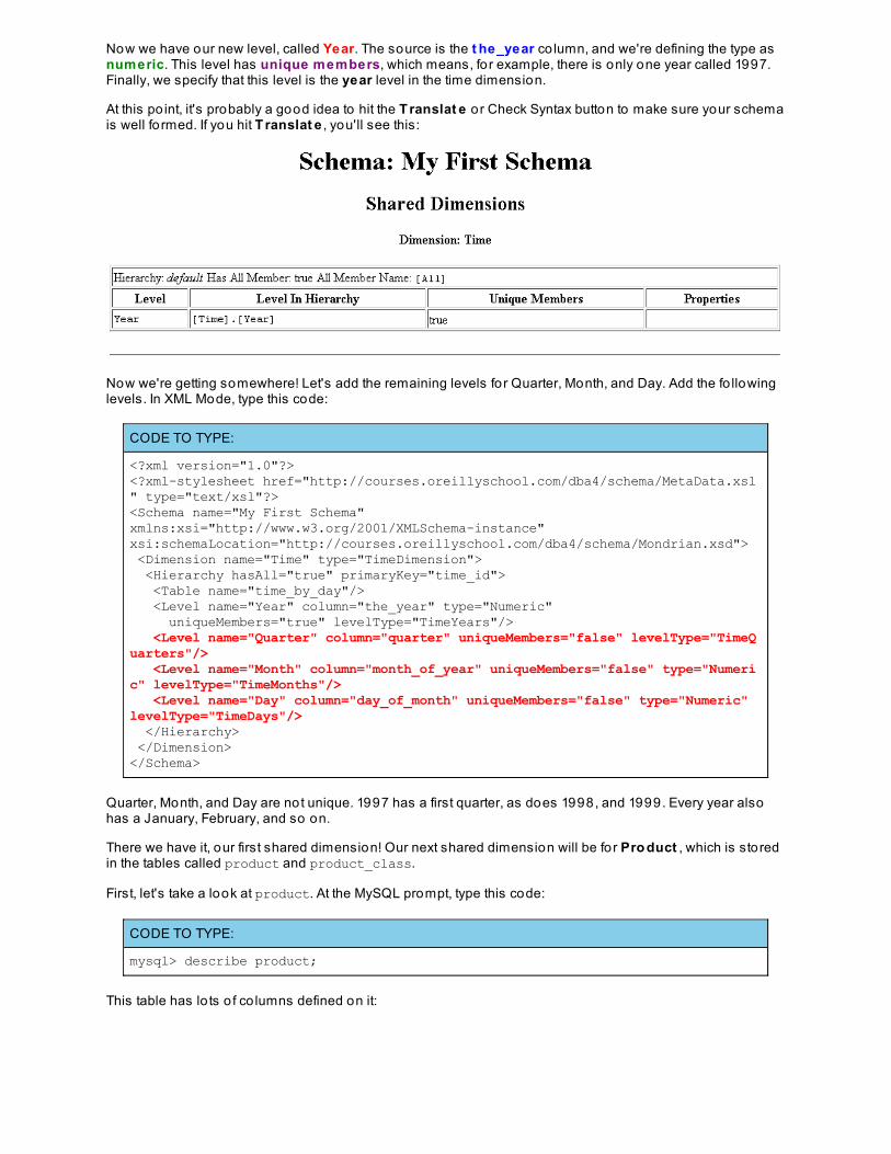
Now we have our new level, called Year. The source is the t he_year co lumn, and we're defining the type asnumeric. This level has unique members, which means, fo r example, there is only one year called 1997.Finally, we specify that this level is the year level in the time dimension.
At this po int, it's probably a good idea to hit the T ranslat e o r Check Syntax button to make sure your schemais well fo rmed. If you hit T ranslat e , you'll see this:
Now we're getting somewhere! Let's add the remaining levels fo r Quarter, Month, and Day. Add the fo llowinglevels. In XML Mode, type this code:
CODE TO TYPE:
<?xml version="1.0"?><?xml-stylesheet href="http://courses.oreillyschool.com/dba4/schema/MetaData.xsl" type="text/xsl"?><Schema name="My First Schema"xmlns:xsi="http://www.w3.org/2001/XMLSchema-instance"xsi:schemaLocation="http://courses.oreillyschool.com/dba4/schema/Mondrian.xsd"> <Dimension name="Time" type="TimeDimension"> <Hierarchy hasAll="true" primaryKey="time_id"> <Table name="time_by_day"/> <Level name="Year" column="the_year" type="Numeric" uniqueMembers="true" levelType="TimeYears"/> <Level name="Quarter" column="quarter" uniqueMembers="false" levelType="TimeQuarters"/> <Level name="Month" column="month_of_year" uniqueMembers="false" type="Numeric" levelType="TimeMonths"/> <Level name="Day" column="day_of_month" uniqueMembers="false" type="Numeric" levelType="TimeDays"/> </Hierarchy> </Dimension></Schema>
Quarter, Month, and Day are not unique. 1997 has a first quarter, as does 1998, and 1999. Every year alsohas a January, February, and so on.
There we have it, our first shared dimension! Our next shared dimension will be for Pro duct , which is storedin the tables called product and product_class.
First, let's take a look at product. At the MySQL prompt, type this code:
CODE TO TYPE:
mysql> describe product;
This table has lo ts o f co lumns defined on it:

OBSERVE:
mysql> describe product;+--------------------+---------------+------+-----+---------+-------+| Field | Type | Null | Key | Default | Extra |+--------------------+---------------+------+-----+---------+-------+| product_class_id | int(11) | NO | MUL | NULL | | | product_id | int(11) | NO | PRI | NULL | | | brand_name | varchar(60) | YES | MUL | NULL | | | product_name | varchar(60) | NO | MUL | NULL | | | SKU | bigint(20) | NO | MUL | NULL | | | SRP | decimal(10,4) | YES | | NULL | | | gross_weight | double | YES | | NULL | | | net_weight | double | YES | | NULL | | | recyclable_package | tinyint(1) | YES | | NULL | | | low_fat | tinyint(1) | YES | | NULL | | | units_per_case | smallint(6) | YES | | NULL | | | cases_per_pallet | smallint(6) | YES | | NULL | | | shelf_width | double | YES | | NULL | | | shelf_height | double | YES | | NULL | | | shelf_depth | double | YES | | NULL | | +--------------------+---------------+------+-----+---------+-------+15 rows in set (0.00 sec)
mysql>
Next, take a look at product_class. At the MySQL prompt, type this:
CODE TO TYPE:
mysql> describe product_class;
This is where the product categories and sub-categories are defined:
OBSERVE:
mysql> describe product_class;+---------------------+-------------+------+-----+---------+-------+| Field | Type | Null | Key | Default | Extra |+---------------------+-------------+------+-----+---------+-------+| product_class_id | int(11) | NO | | NULL | | | product_subcategory | varchar(30) | YES | | NULL | | | product_category | varchar(30) | YES | | NULL | | | product_department | varchar(30) | YES | | NULL | | | product_family | varchar(30) | YES | | NULL | | +---------------------+-------------+------+-----+---------+-------+5 rows in set (0.00 sec)
mysql>
These two tables are jo ined by the product_class_id co lumn. Fortunately, as we'll soon see, Mondrian'sschema allows us to specify how these tables are jo ined together.
To get started, let's add a new shared dimension to our existing schema. In XML Mode, type this code:
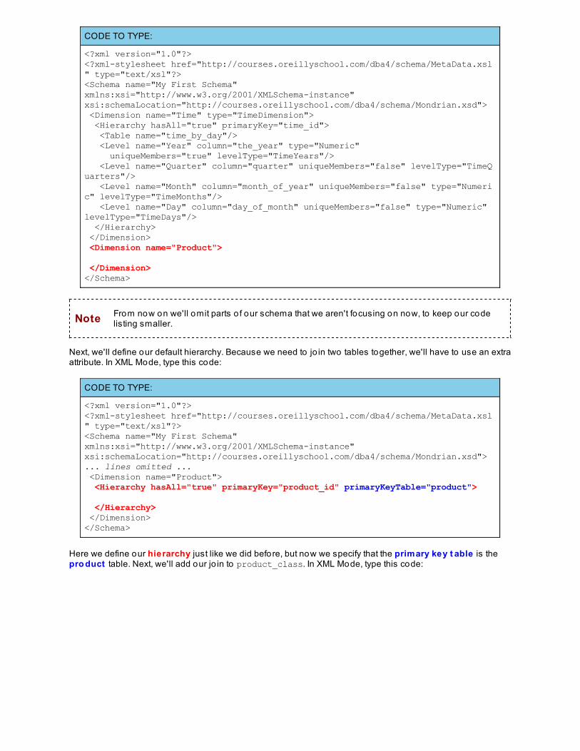
CODE TO TYPE:
<?xml version="1.0"?><?xml-stylesheet href="http://courses.oreillyschool.com/dba4/schema/MetaData.xsl" type="text/xsl"?><Schema name="My First Schema"xmlns:xsi="http://www.w3.org/2001/XMLSchema-instance"xsi:schemaLocation="http://courses.oreillyschool.com/dba4/schema/Mondrian.xsd"> <Dimension name="Time" type="TimeDimension"> <Hierarchy hasAll="true" primaryKey="time_id"> <Table name="time_by_day"/> <Level name="Year" column="the_year" type="Numeric" uniqueMembers="true" levelType="TimeYears"/> <Level name="Quarter" column="quarter" uniqueMembers="false" levelType="TimeQuarters"/> <Level name="Month" column="month_of_year" uniqueMembers="false" type="Numeric" levelType="TimeMonths"/> <Level name="Day" column="day_of_month" uniqueMembers="false" type="Numeric" levelType="TimeDays"/> </Hierarchy> </Dimension> <Dimension name="Product"> </Dimension></Schema>
Note From now on we'll omit parts o f our schema that we aren't focusing on now, to keep our codelisting smaller.
Next, we'll define our default hierarchy. Because we need to jo in two tables together, we'll have to use an extraattribute. In XML Mode, type this code:
CODE TO TYPE:
<?xml version="1.0"?><?xml-stylesheet href="http://courses.oreillyschool.com/dba4/schema/MetaData.xsl" type="text/xsl"?><Schema name="My First Schema"xmlns:xsi="http://www.w3.org/2001/XMLSchema-instance"xsi:schemaLocation="http://courses.oreillyschool.com/dba4/schema/Mondrian.xsd">... lines omitted ... <Dimension name="Product"> <Hierarchy hasAll="true" primaryKey="product_id" primaryKeyTable="product"> </Hierarchy> </Dimension></Schema>
Here we define our hierarchy just like we did before, but now we specify that the primary key t able is thepro duct table. Next, we'll add our jo in to product_class. In XML Mode, type this code:

CODE TO TYPE:
<?xml version="1.0"?><?xml-stylesheet href="http://courses.oreillyschool.com/dba4/schema/MetaData.xsl" type="text/xsl"?><Schema name="My First Schema"xmlns:xsi="http://www.w3.org/2001/XMLSchema-instance"xsi:schemaLocation="http://courses.oreillyschool.com/dba4/schema/Mondrian.xsd">... lines omitted ... <Dimension name="Product"> <Hierarchy hasAll="true" primaryKey="product_id" primaryKeyTable="product"> <Join leftKey="product_class_id" rightKey="product_class_id"> <Table name="product"/> <Table name="product_class"/> </Join> </Hierarchy> </Dimension></Schema>
The jo in code is a long-winded way o f specifying the SQL jo in between pro duct and pro duct _class, usingthe co lumn product_class_id from both tables.
Next, we define the levels fo r our hierarchy. The product dimension has the fo llowing hierarchy and levelsdefined:
OBSERVE:
Product Family Product Department Product Category Product Subcategory Brand Name Product Name
We can define the levels fo r this dimension just like we did for the last dimension. The only difference is thatwe need to add an attribute for t able . In XML Mode, type this code:
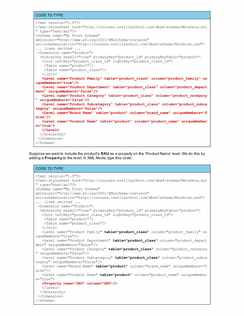
CODE TO TYPE:
<?xml version="1.0"?><?xml-stylesheet href="http://courses.oreillyschool.com/dba4/schema/MetaData.xsl" type="text/xsl"?><Schema name="My First Schema"xmlns:xsi="http://www.w3.org/2001/XMLSchema-instance"xsi:schemaLocation="http://courses.oreillyschool.com/dba4/schema/Mondrian.xsd">... lines omitted ... <Dimension name="Product"> <Hierarchy hasAll="true" primaryKey="product_id" primaryKeyTable="product"> <Join leftKey="product_class_id" rightKey="product_class_id"> <Table name="product"/> <Table name="product_class"/> </Join> <Level name="Product Family" table="product_class" column="product_family" uniqueMembers="true"/> <Level name="Product Department" table="product_class" column="product_department" uniqueMembers="false"/> <Level name="Product Category" table="product_class" column="product_category" uniqueMembers="false"/> <Level name="Product Subcategory" table="product_class" column="product_subcategory" uniqueMembers="false"/> <Level name="Brand Name" table="product" column="brand_name" uniqueMembers="false"/> <Level name="Product Name" table="product" column="product_name" uniqueMembers="true"> </Level> </Hierarchy> </Dimension></Schema>
Suppose we want to include the product's SKU as a property on the 'Product Name' level. We do this byadding a Pro pert y to the level. In XML Mode, type this code:
CODE TO TYPE:
<?xml version="1.0"?><?xml-stylesheet href="http://courses.oreillyschool.com/dba4/schema/MetaData.xsl" type="text/xsl"?><Schema name="My First Schema"xmlns:xsi="http://www.w3.org/2001/XMLSchema-instance"xsi:schemaLocation="http://courses.oreillyschool.com/dba4/schema/Mondrian.xsd">... lines omitted ... <Dimension name="Product"> <Hierarchy hasAll="true" primaryKey="product_id" primaryKeyTable="product"> <Join leftKey="product_class_id" rightKey="product_class_id"> <Table name="product"/> <Table name="product_class"/> </Join> <Level name="Product Family" table="product_class" column="product_family" uniqueMembers="true"/> <Level name="Product Department" table="product_class" column="product_department" uniqueMembers="false"/> <Level name="Product Category" table="product_class" column="product_category" uniqueMembers="false"/> <Level name="Product Subcategory" table="product_class" column="product_subcategory" uniqueMembers="false"/> <Level name="Brand Name" table="product" column="brand_name" uniqueMembers="false"/> <Level name="Product Name" table="product" column="product_name" uniqueMembers="true"> <Property name="SKU" column="SKU"/> </Level> </Hierarchy> </Dimension></Schema>
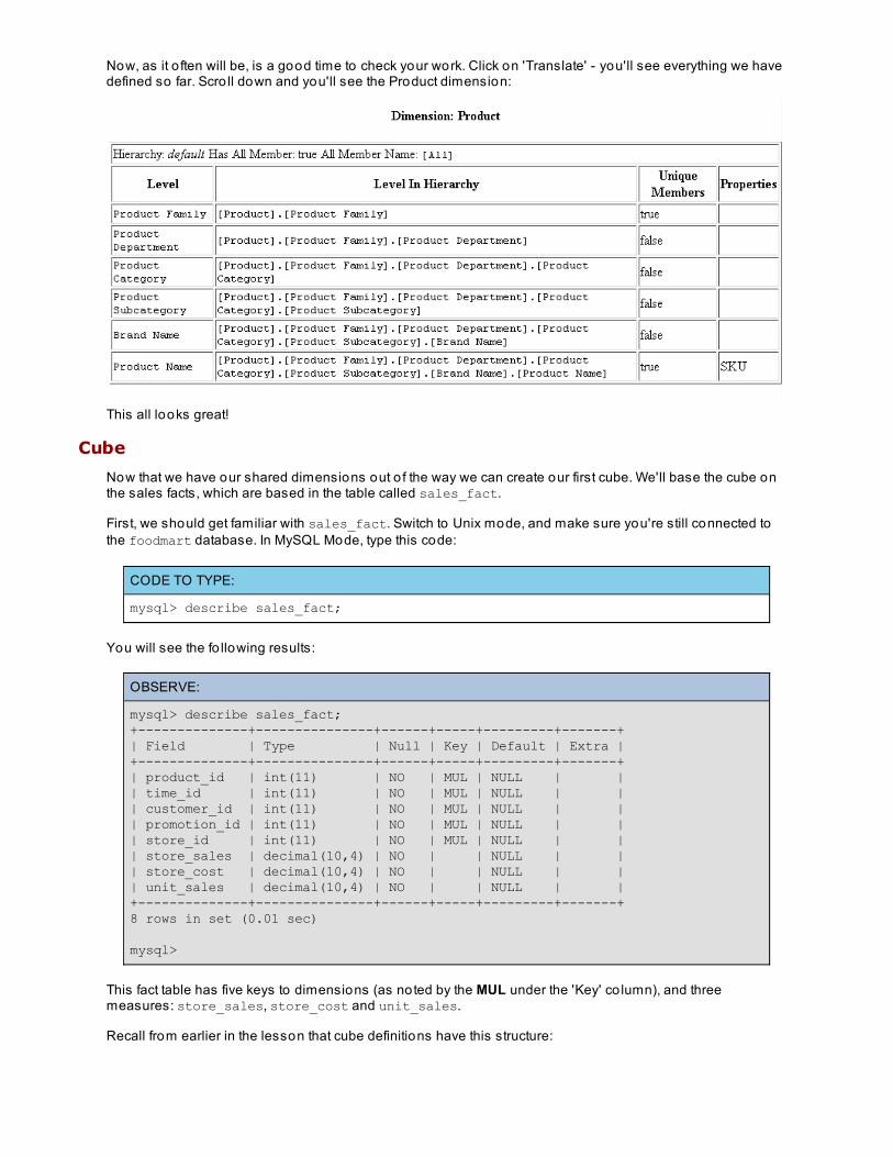
Now, as it o ften will be, is a good time to check your work. Click on 'Translate' - you'll see everything we havedefined so far. Scro ll down and you'll see the Product dimension:
This all looks great!
Cube
Now that we have our shared dimensions out o f the way we can create our first cube. We'll base the cube onthe sales facts, which are based in the table called sales_fact.
First, we should get familiar with sales_fact. Switch to Unix mode, and make sure you're still connected tothe foodmart database. In MySQL Mode, type this code:
CODE TO TYPE:
mysql> describe sales_fact;
You will see the fo llowing results:
OBSERVE:
mysql> describe sales_fact;+--------------+---------------+------+-----+---------+-------+| Field | Type | Null | Key | Default | Extra |+--------------+---------------+------+-----+---------+-------+| product_id | int(11) | NO | MUL | NULL | | | time_id | int(11) | NO | MUL | NULL | | | customer_id | int(11) | NO | MUL | NULL | | | promotion_id | int(11) | NO | MUL | NULL | | | store_id | int(11) | NO | MUL | NULL | | | store_sales | decimal(10,4) | NO | | NULL | | | store_cost | decimal(10,4) | NO | | NULL | | | unit_sales | decimal(10,4) | NO | | NULL | | +--------------+---------------+------+-----+---------+-------+8 rows in set (0.01 sec)
mysql>
This fact table has five keys to dimensions (as noted by the MUL under the 'Key' co lumn), and threemeasures: store_sales, store_cost and unit_sales.
Recall from earlier in the lesson that cube definitions have this structure:
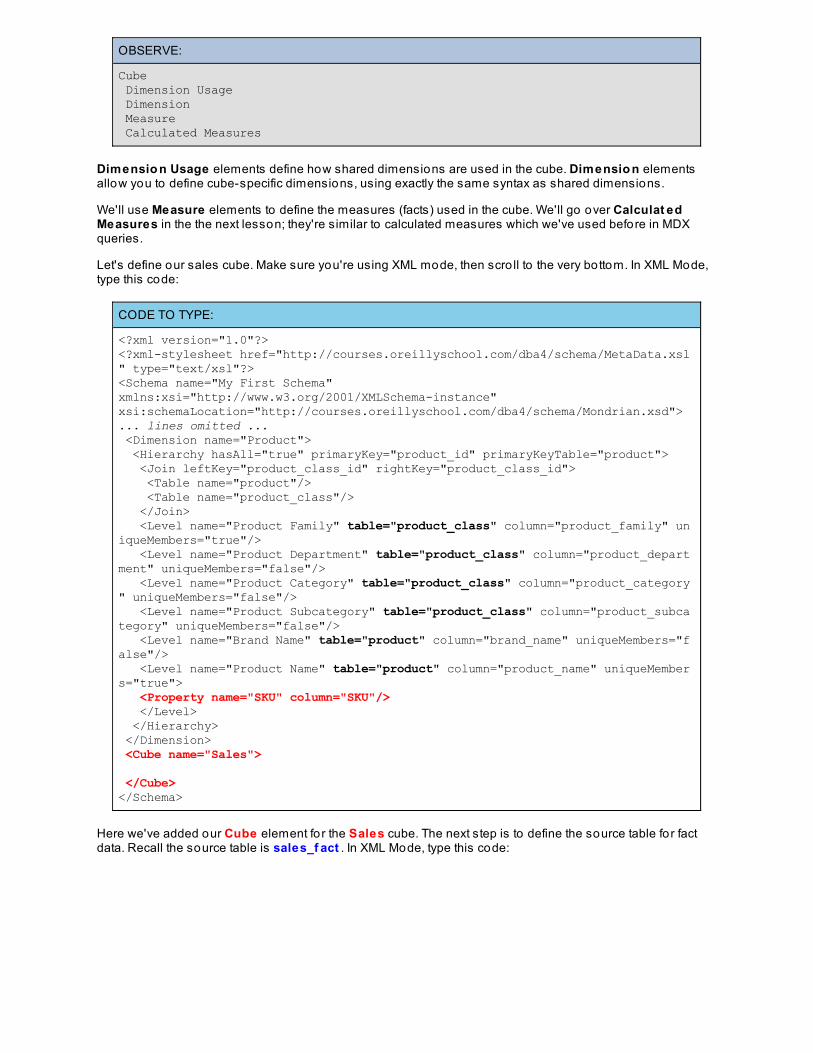
OBSERVE:
Cube Dimension Usage Dimension Measure Calculated Measures
Dimensio n Usage elements define how shared dimensions are used in the cube. Dimensio n elementsallow you to define cube-specific dimensions, using exactly the same syntax as shared dimensions.
We'll use Measure elements to define the measures (facts) used in the cube. We'll go over Calculat edMeasures in the the next lesson; they're similar to calculated measures which we've used before in MDXqueries.
Let's define our sales cube. Make sure you're using XML mode, then scro ll to the very bottom. In XML Mode,type this code:
CODE TO TYPE:
<?xml version="1.0"?><?xml-stylesheet href="http://courses.oreillyschool.com/dba4/schema/MetaData.xsl" type="text/xsl"?><Schema name="My First Schema"xmlns:xsi="http://www.w3.org/2001/XMLSchema-instance"xsi:schemaLocation="http://courses.oreillyschool.com/dba4/schema/Mondrian.xsd">... lines omitted ... <Dimension name="Product"> <Hierarchy hasAll="true" primaryKey="product_id" primaryKeyTable="product"> <Join leftKey="product_class_id" rightKey="product_class_id"> <Table name="product"/> <Table name="product_class"/> </Join> <Level name="Product Family" table="product_class" column="product_family" uniqueMembers="true"/> <Level name="Product Department" table="product_class" column="product_department" uniqueMembers="false"/> <Level name="Product Category" table="product_class" column="product_category" uniqueMembers="false"/> <Level name="Product Subcategory" table="product_class" column="product_subcategory" uniqueMembers="false"/> <Level name="Brand Name" table="product" column="brand_name" uniqueMembers="false"/> <Level name="Product Name" table="product" column="product_name" uniqueMembers="true"> <Property name="SKU" column="SKU"/> </Level> </Hierarchy> </Dimension> <Cube name="Sales"> </Cube></Schema>
Here we've added our Cube element fo r the Sales cube. The next step is to define the source table for factdata. Recall the source table is sales_f act . In XML Mode, type this code:
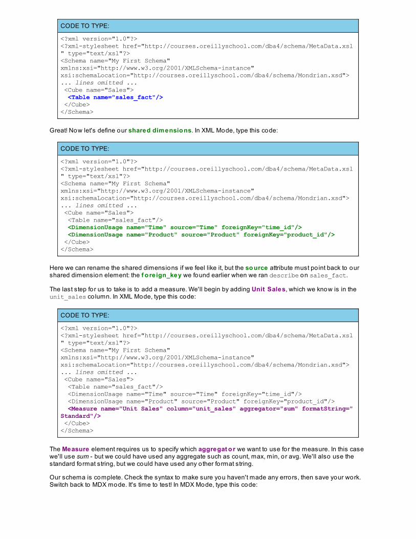
CODE TO TYPE:
<?xml version="1.0"?><?xml-stylesheet href="http://courses.oreillyschool.com/dba4/schema/MetaData.xsl" type="text/xsl"?><Schema name="My First Schema"xmlns:xsi="http://www.w3.org/2001/XMLSchema-instance"xsi:schemaLocation="http://courses.oreillyschool.com/dba4/schema/Mondrian.xsd">... lines omitted ... <Cube name="Sales"> <Table name="sales_fact"/> </Cube></Schema>
Great! Now let's define our shared dimensio ns. In XML Mode, type this code:
CODE TO TYPE:
<?xml version="1.0"?><?xml-stylesheet href="http://courses.oreillyschool.com/dba4/schema/MetaData.xsl" type="text/xsl"?><Schema name="My First Schema"xmlns:xsi="http://www.w3.org/2001/XMLSchema-instance"xsi:schemaLocation="http://courses.oreillyschool.com/dba4/schema/Mondrian.xsd">... lines omitted ... <Cube name="Sales"> <Table name="sales_fact"/> <DimensionUsage name="Time" source="Time" foreignKey="time_id"/> <DimensionUsage name="Product" source="Product" foreignKey="product_id"/> </Cube></Schema>
Here we can rename the shared dimensions if we feel like it, but the so urce attribute must po int back to ourshared dimension element: the f o reign_key we found earlier when we ran describe on sales_fact.
The last step for us to take is to add a measure. We'll begin by adding Unit Sales, which we know is in theunit_sales co lumn. In XML Mode, type this code:
CODE TO TYPE:
<?xml version="1.0"?><?xml-stylesheet href="http://courses.oreillyschool.com/dba4/schema/MetaData.xsl" type="text/xsl"?><Schema name="My First Schema"xmlns:xsi="http://www.w3.org/2001/XMLSchema-instance"xsi:schemaLocation="http://courses.oreillyschool.com/dba4/schema/Mondrian.xsd">... lines omitted ... <Cube name="Sales"> <Table name="sales_fact"/> <DimensionUsage name="Time" source="Time" foreignKey="time_id"/> <DimensionUsage name="Product" source="Product" foreignKey="product_id"/> <Measure name="Unit Sales" column="unit_sales" aggregator="sum" formatString="Standard"/> </Cube></Schema>
The Measure element requires us to specify which aggregat o r we want to use for the measure. In this casewe'll use sum - but we could have used any aggregate such as count, max, min, or avg. We'll also use thestandard format string, but we could have used any o ther fo rmat string.
Our schema is complete. Check the syntax to make sure you haven't made any errors, then save your work.Switch back to MDX mode. It's time to test! In MDX Mode, type this code:
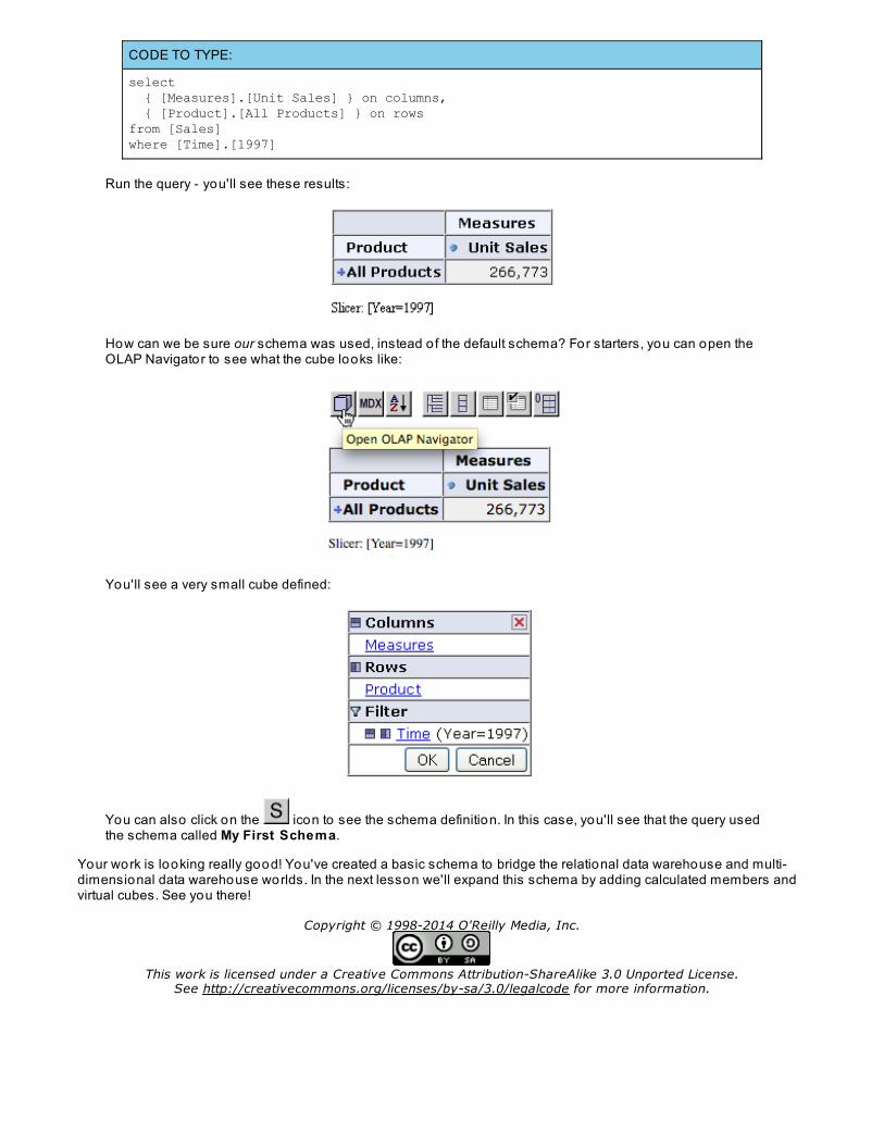
CODE TO TYPE:
select { [Measures].[Unit Sales] } on columns, { [Product].[All Products] } on rowsfrom [Sales]where [Time].[1997]
Run the query - you'll see these results:
How can we be sure our schema was used, instead o f the default schema? For starters, you can open theOLAP Navigator to see what the cube looks like:
You'll see a very small cube defined:
You can also click on the icon to see the schema definition. In this case, you'll see that the query usedthe schema called My First Schema.
Your work is looking really good! You've created a basic schema to bridge the relational data warehouse and multi-dimensional data warehouse worlds. In the next lesson we'll expand this schema by adding calculated members andvirtual cubes. See you there!
Copyright © 1998-2014 O'Reilly Media, Inc.
This work is licensed under a Creative Commons Attribution-ShareAlike 3.0 Unported License.See http://creativecommons.org/licenses/by-sa/3.0/legalcode for more information.
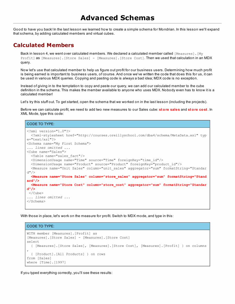
Advanced Schemas
Good to have you back! In the last lesson we learned how to create a simple schema for Mondrian. In this lesson we'll expandthat schema, by adding calculated members and virtual cubes.
Calculated MembersBack in lesson 4, we went over calculated members. We declared a calculated member called [Measures].[MyProfit] as [Measures].[Store Sales] - [Measures].[Store Cost]. Then we used that calculation in an MDXquery.
Now let's use that calculated member to help us figure out pro fit fo r our business users. Determining how much pro fitis being earned is important to business users, o f course. And once we've written the code that does this fo r us, it canbe used in various MDX queries. Copying and pasting code is always a bad idea; MDX code is no exception.
Instead o f giving in to the temptation to copy and paste our query, we can add our calculated member to the cubedefinition in the schema. This makes the member available to anyone who uses MDX. Nobody even has to know it is acalculated member!
Let's try this stuff out. To get started, open the schema that we worked on in the last lesson (including the pro jects).
Before we can calculate pro fit, we need to add two new measures to our Sales cube: st o re sales and st o re co st . InXML Mode, type this code:
CODE TO TYPE:
<?xml version="1.0"?> <?xml-stylesheet href="http://courses.oreillyschool.com/dba4/schema/MetaData.xsl" type="text/xsl"?><Schema name="My First Schema">... lines omitted ... <Cube name="Sales"> <Table name="sales_fact"/> <DimensionUsage name="Time" source="Time" foreignKey="time_id"/> <DimensionUsage name="Product" source="Product" foreignKey="product_id"/> <Measure name="Unit Sales" column="unit_sales" aggregator="sum" formatString="Standard"/> <Measure name="Store Sales" column="store_sales" aggregator="sum" formatString="Standard"/> <Measure name="Store Cost" column="store_cost" aggregator="sum" formatString="Standard"/> </Cube>... lines omitted ... </Schema>
With those in place, let's work on the measure for pro fit. Switch to MDX mode, and type in this:
CODE TO TYPE:
WITH member [Measures].[Profit] as [Measures].[Store Sales] - [Measures].[Store Cost]select { [Measures].[Store Sales], [Measures].[Store Cost], [Measures].[Profit] } on columns, { [Product].[All Products] } on rowsfrom [Sales]where [Time].[1997]
If you typed everything correctly, you'll see these results:
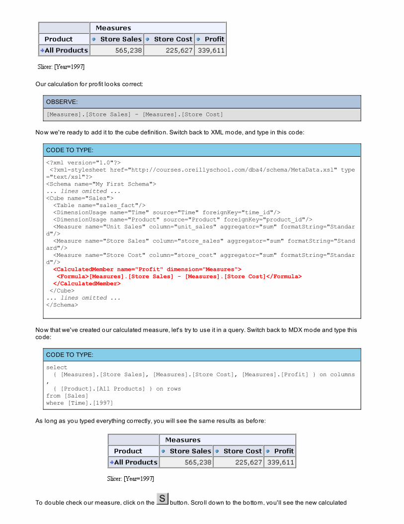
Our calculation for pro fit looks correct:
OBSERVE:
[Measures].[Store Sales] - [Measures].[Store Cost]
Now we're ready to add it to the cube definition. Switch back to XML mode, and type in this code:
CODE TO TYPE:
<?xml version="1.0"?> <?xml-stylesheet href="http://courses.oreillyschool.com/dba4/schema/MetaData.xsl" type="text/xsl"?><Schema name="My First Schema">... lines omitted ... <Cube name="Sales"> <Table name="sales_fact"/> <DimensionUsage name="Time" source="Time" foreignKey="time_id"/> <DimensionUsage name="Product" source="Product" foreignKey="product_id"/> <Measure name="Unit Sales" column="unit_sales" aggregator="sum" formatString="Standard"/> <Measure name="Store Sales" column="store_sales" aggregator="sum" formatString="Standard"/> <Measure name="Store Cost" column="store_cost" aggregator="sum" formatString="Standard"/> <CalculatedMember name="Profit" dimension="Measures"> <Formula>[Measures].[Store Sales] - [Measures].[Store Cost]</Formula> </CalculatedMember> </Cube>... lines omitted ... </Schema>
Now that we've created our calculated measure, let's try to use it in a query. Switch back to MDX mode and type thiscode:
CODE TO TYPE:
select { [Measures].[Store Sales], [Measures].[Store Cost], [Measures].[Profit] } on columns, { [Product].[All Products] } on rowsfrom [Sales]where [Time].[1997]
As long as you typed everything correctly, you will see the same results as before:
To double check our measure, click on the button. Scro ll down to the bottom, you'll see the new calculated
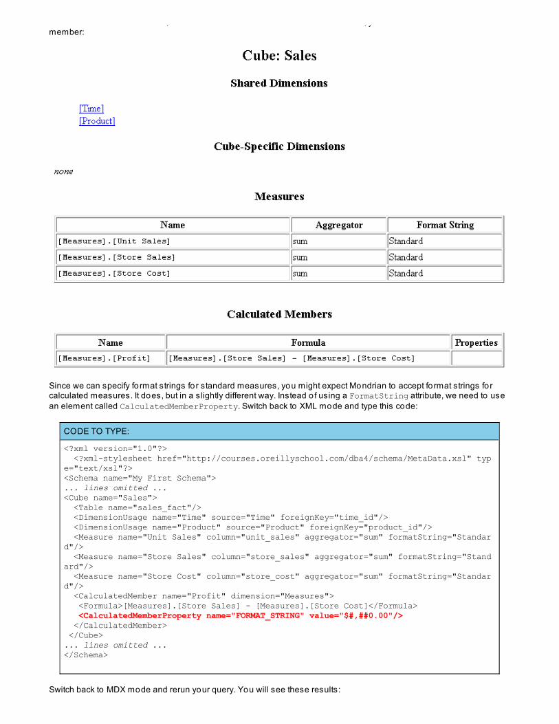
To double check our measure, click on the button. Scro ll down to the bottom, you'll see the new calculatedmember:
Since we can specify fo rmat strings for standard measures, you might expect Mondrian to accept fo rmat strings forcalculated measures. It does, but in a slightly different way. Instead o f using a FormatString attribute, we need to usean element called CalculatedMemberProperty. Switch back to XML mode and type this code:
CODE TO TYPE:
<?xml version="1.0"?> <?xml-stylesheet href="http://courses.oreillyschool.com/dba4/schema/MetaData.xsl" type="text/xsl"?> <Schema name="My First Schema">... lines omitted ... <Cube name="Sales"> <Table name="sales_fact"/> <DimensionUsage name="Time" source="Time" foreignKey="time_id"/> <DimensionUsage name="Product" source="Product" foreignKey="product_id"/> <Measure name="Unit Sales" column="unit_sales" aggregator="sum" formatString="Standard"/> <Measure name="Store Sales" column="store_sales" aggregator="sum" formatString="Standard"/> <Measure name="Store Cost" column="store_cost" aggregator="sum" formatString="Standard"/> <CalculatedMember name="Profit" dimension="Measures"> <Formula>[Measures].[Store Sales] - [Measures].[Store Cost]</Formula> <CalculatedMemberProperty name="FORMAT_STRING" value="$#,##0.00"/> </CalculatedMember> </Cube>... lines omitted ... </Schema>
Switch back to MDX mode and rerun your query. You will see these results:
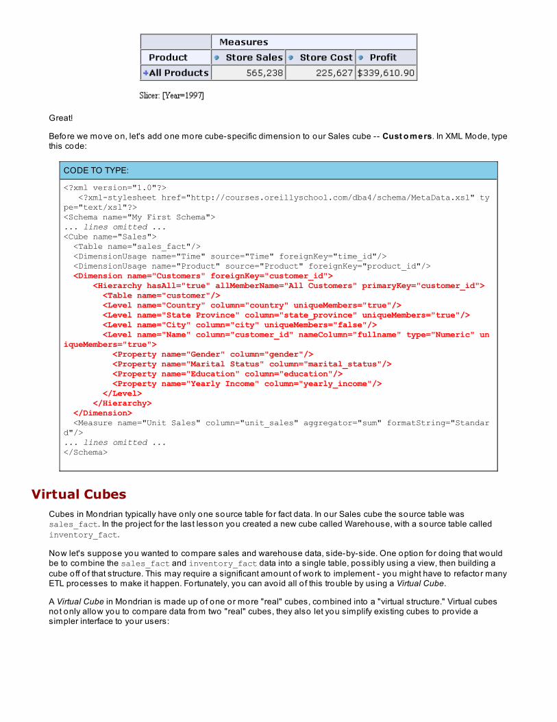
Great!
Before we move on, let's add one more cube-specific dimension to our Sales cube -- Cust o mers. In XML Mode, typethis code:
CODE TO TYPE:
<?xml version="1.0"?> <?xml-stylesheet href="http://courses.oreillyschool.com/dba4/schema/MetaData.xsl" type="text/xsl"?> <Schema name="My First Schema">... lines omitted ... <Cube name="Sales"> <Table name="sales_fact"/> <DimensionUsage name="Time" source="Time" foreignKey="time_id"/> <DimensionUsage name="Product" source="Product" foreignKey="product_id"/> <Dimension name="Customers" foreignKey="customer_id"> <Hierarchy hasAll="true" allMemberName="All Customers" primaryKey="customer_id"> <Table name="customer"/> <Level name="Country" column="country" uniqueMembers="true"/> <Level name="State Province" column="state_province" uniqueMembers="true"/> <Level name="City" column="city" uniqueMembers="false"/> <Level name="Name" column="customer_id" nameColumn="fullname" type="Numeric" uniqueMembers="true"> <Property name="Gender" column="gender"/> <Property name="Marital Status" column="marital_status"/> <Property name="Education" column="education"/> <Property name="Yearly Income" column="yearly_income"/> </Level> </Hierarchy> </Dimension> <Measure name="Unit Sales" column="unit_sales" aggregator="sum" formatString="Standard"/>... lines omitted ... </Schema>
Virtual CubesCubes in Mondrian typically have only one source table for fact data. In our Sales cube the source table wassales_fact. In the pro ject fo r the last lesson you created a new cube called Warehouse, with a source table calledinventory_fact.
Now let's suppose you wanted to compare sales and warehouse data, side-by-side. One option for do ing that wouldbe to combine the sales_fact and inventory_fact data into a single table, possibly using a view, then building acube o ff o f that structure. This may require a significant amount o f work to implement - you might have to refactor manyETL processes to make it happen. Fortunately, you can avo id all o f this trouble by using a Virtual Cube.
A Virtual Cube in Mondrian is made up o f one or more "real" cubes, combined into a "virtual structure." Virtual cubesnot only allow you to compare data from two "real" cubes, they also let you simplify existing cubes to provide asimpler interface to your users:
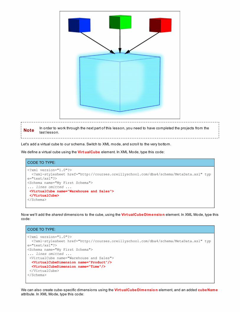
Note In order to work through the next part o f this lesson, you need to have completed the pro jects from thelast lesson.
Let's add a virtual cube to our schema. Switch to XML mode, and scro ll to the very bottom.
We define a virtual cube using the Virt ualCube element. In XML Mode, type this code:
CODE TO TYPE:
<?xml version="1.0"?> <?xml-stylesheet href="http://courses.oreillyschool.com/dba4/schema/MetaData.xsl" type="text/xsl"?> <Schema name="My First Schema">... lines omitted ... <VirtualCube name="Warehouse and Sales"> </VirtualCube></Schema>
Now we'll add the shared dimensions to the cube, using the Virt ualCubeDimensio n element. In XML Mode, type thiscode:
CODE TO TYPE:
<?xml version="1.0"?> <?xml-stylesheet href="http://courses.oreillyschool.com/dba4/schema/MetaData.xsl" type="text/xsl"?> <Schema name="My First Schema">... lines omitted ... <VirtualCube name="Warehouse and Sales"> <VirtualCubeDimension name="Product"/> <VirtualCubeDimension name="Time"/> </VirtualCube></Schema>
We can also create cube-specific dimensions using the Virt ualCubeDimensio n element, and an added cubeNameattribute. In XML Mode, type this code:
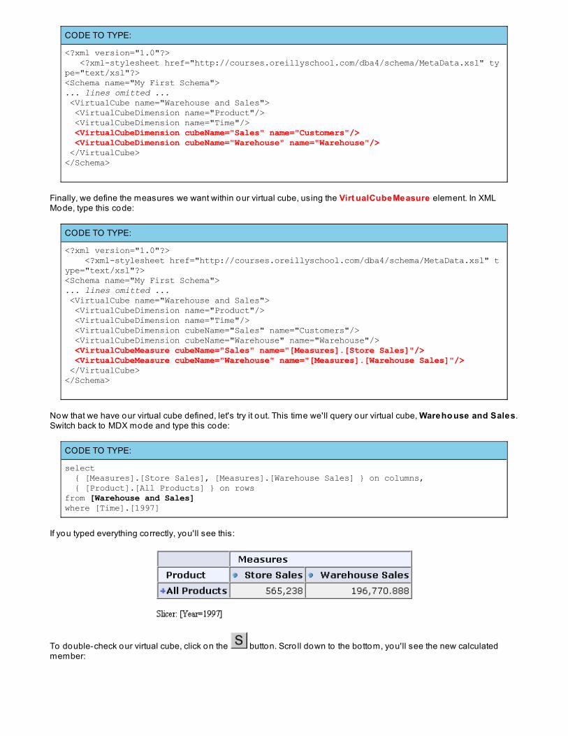
CODE TO TYPE:
<?xml version="1.0"?> <?xml-stylesheet href="http://courses.oreillyschool.com/dba4/schema/MetaData.xsl" type="text/xsl"?> <Schema name="My First Schema">... lines omitted ... <VirtualCube name="Warehouse and Sales"> <VirtualCubeDimension name="Product"/> <VirtualCubeDimension name="Time"/> <VirtualCubeDimension cubeName="Sales" name="Customers"/> <VirtualCubeDimension cubeName="Warehouse" name="Warehouse"/> </VirtualCube></Schema>
Finally, we define the measures we want within our virtual cube, using the Virt ualCubeMeasure element. In XMLMode, type this code:
CODE TO TYPE:
<?xml version="1.0"?> <?xml-stylesheet href="http://courses.oreillyschool.com/dba4/schema/MetaData.xsl" type="text/xsl"?> <Schema name="My First Schema">... lines omitted ... <VirtualCube name="Warehouse and Sales"> <VirtualCubeDimension name="Product"/> <VirtualCubeDimension name="Time"/> <VirtualCubeDimension cubeName="Sales" name="Customers"/> <VirtualCubeDimension cubeName="Warehouse" name="Warehouse"/> <VirtualCubeMeasure cubeName="Sales" name="[Measures].[Store Sales]"/> <VirtualCubeMeasure cubeName="Warehouse" name="[Measures].[Warehouse Sales]"/> </VirtualCube></Schema>
Now that we have our virtual cube defined, let's try it out. This time we'll query our virtual cube, Wareho use and Sales.Switch back to MDX mode and type this code:
CODE TO TYPE:
select { [Measures].[Store Sales], [Measures].[Warehouse Sales] } on columns, { [Product].[All Products] } on rowsfrom [Warehouse and Sales]where [Time].[1997]
If you typed everything correctly, you'll see this:
To double-check our virtual cube, click on the button. Scro ll down to the bottom, you'll see the new calculatedmember:
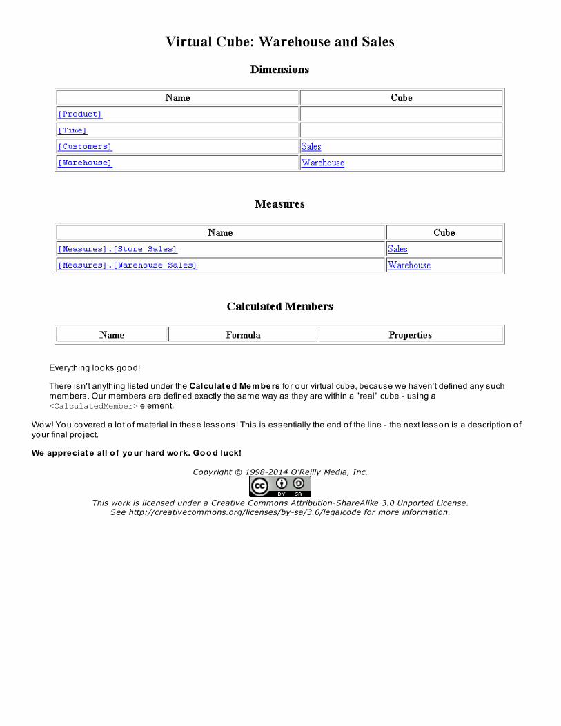
Everything looks good!
There isn't anything listed under the Calculat ed Members fo r our virtual cube, because we haven't defined any suchmembers. Our members are defined exactly the same way as they are within a "real" cube - using a<CalculatedMember> element.
Wow! You covered a lo t o f material in these lessons! This is essentially the end o f the line - the next lesson is a description o fyour final pro ject.
We appreciat e all o f yo ur hard wo rk. Go o d luck!
Copyright © 1998-2014 O'Reilly Media, Inc.
This work is licensed under a Creative Commons Attribution-ShareAlike 3.0 Unported License.See http://creativecommons.org/licenses/by-sa/3.0/legalcode for more information.
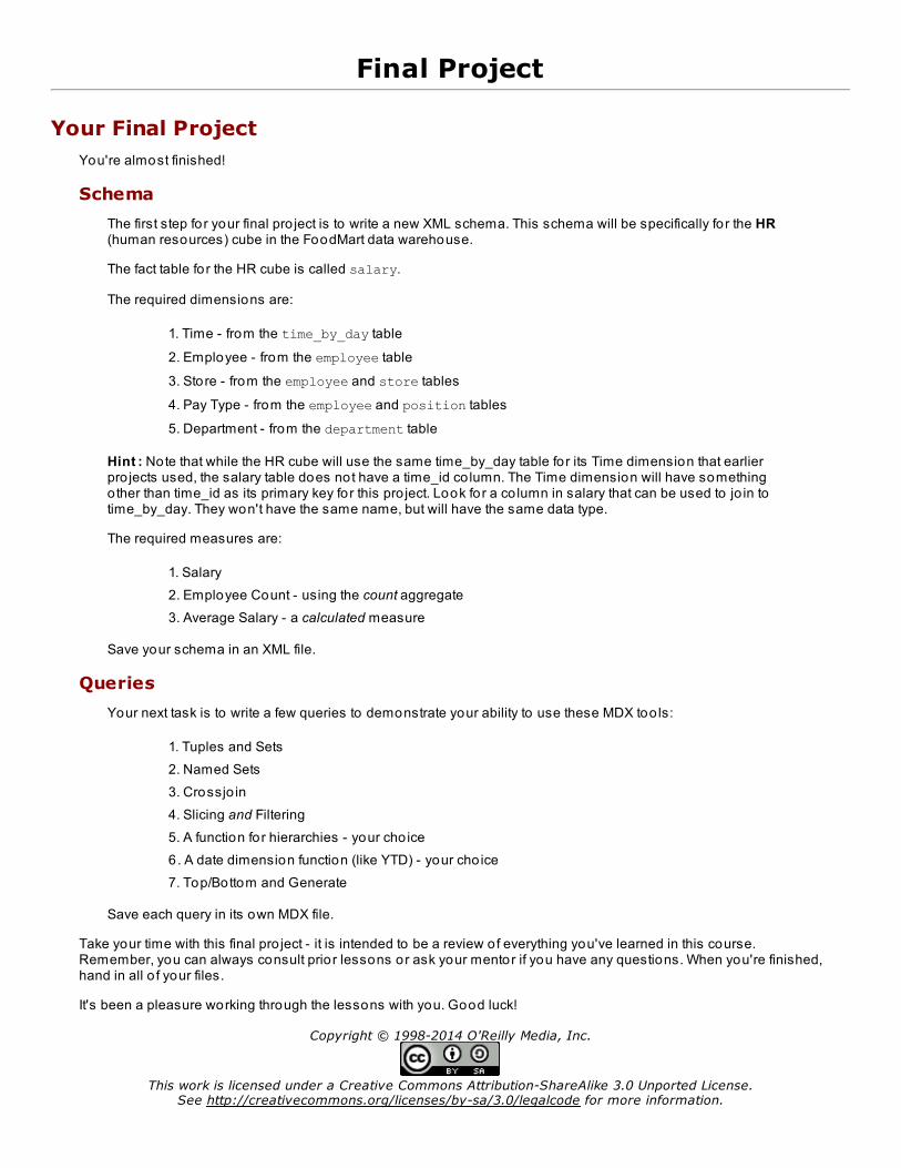
Final Project
Your Final ProjectYou're almost finished!
Schema
The first step for your final pro ject is to write a new XML schema. This schema will be specifically fo r the HR(human resources) cube in the FoodMart data warehouse.
The fact table for the HR cube is called salary.
The required dimensions are:
1. Time - from the time_by_day table
2. Employee - from the employee table
3. Store - from the employee and store tables
4. Pay Type - from the employee and position tables
5. Department - from the department table
Hint : Note that while the HR cube will use the same time_by_day table for its Time dimension that earlierpro jects used, the salary table does not have a time_id co lumn. The Time dimension will have somethingother than time_id as its primary key for this pro ject. Look for a co lumn in salary that can be used to jo in totime_by_day. They won't have the same name, but will have the same data type.
The required measures are:
1. Salary2. Employee Count - using the count aggregate3. Average Salary - a calculated measure
Save your schema in an XML file.
Queries
Your next task is to write a few queries to demonstrate your ability to use these MDX too ls:
1. Tuples and Sets2. Named Sets3. Crossjo in4. Slicing and Filtering5. A function for hierarchies - your cho ice6. A date dimension function (like YTD) - your cho ice7. Top/Bottom and Generate
Save each query in its own MDX file.
Take your time with this final pro ject - it is intended to be a review of everything you've learned in this course.Remember, you can always consult prio r lessons or ask your mentor if you have any questions. When you're finished,hand in all o f your files.
It's been a pleasure working through the lessons with you. Good luck!
Copyright © 1998-2014 O'Reilly Media, Inc.
This work is licensed under a Creative Commons Attribution-ShareAlike 3.0 Unported License.See http://creativecommons.org/licenses/by-sa/3.0/legalcode for more information.