database management systemsiare.ac.in/sites/default/files/ppt/iare_dbms_ppt_0.pdfdatabase management...
TRANSCRIPT

Database Management Systems

UNIT - I

CONCEPTUAL MODELING
Introduction to DBMS- Data, Information,
Database, DBMS

Data:
• Raw facts; building blocks of information
• Unprocessed information
Information:
– Data processed to reveal meaning

Database
Database—shared, integrated computer structure that stores:
– End user data (raw facts)
– Metadata (data about data)

Database management system
• DBMS (Database management system):
– Collection of programs that manages database structure and
controls access to data
– Possible to share data among multiple applications or users
– Makes data management more efficient and effective

Advantages of the DBMS
• End users have better access to more and better-managed data
– Promotes integrated view of organization’s operations
– Probability of data inconsistency is greatly reduced
– Possible to produce quick answers to ad hoc queries

DBMS contains information about a particular enterprise
1. Collection of interrelated data
2. Set of programs to access the data
3. An environment that is both convenient and efficient to use

CONCEPTUAL MODELING
DB Applications, various DBMS

Database Applications
• Database Applications:
– Banking: transactions
– Airlines: reservations, schedules
– Universities: registration, grades
– Sales: customers, products, purchases

Database Applications(contd.)
—Online retailers: order tracking, customized recommendations
—Manufacturing: production, inventory, orders, supply chain
—Human resources: employee records, salaries, tax deductions
• Databases can be very large.
• Databases touch all aspects of our lives

University Database Example
• Application program examples
– Add new students, instructors, and courses
– Register students for courses, and generate class rosters
– Assign grades to students, compute grade point averages (GPA)
and generate transcripts
• In the early days, database applications were built directly on top of
file systems

Various Databases
• Single-user:
– Supports only one user at a time
• Desktop:
– Single-user database running on a personal computer
• Multi-user:
– Supports multiple users at the same time

Various Databases(contd.)
• Workgroup:
– Multi-user database that supports a small group of users or a
single department
• Enterprise:
– Multi-user database that supports a large group of users or an
entire organization

Various Databases(contd.)
Can be classified by location:
• Centralized:
– Supports data located at a single site
• Distributed:
– Supports data distributed across several sites

CONCEPTUAL MODELING
DBMS Vs. File Management
System, Levels of Abstractions,
Data Independence

Drawbacks of file systems
• Data redundancy and inconsistency
– Multiple file formats, duplication of information in different files
• Difficulty in accessing data
– Need to write a new program to carry out each new task
• Data isolation
– Multiple files and formats

Drawbacks of file systems (contd.)
Integrity problems
Integrity constraints (e.g., account balance > 0) become “buried” in program code rather than being stated explicitly
Hard to add new constraints or change existing ones
Atomicity of updates
Failures may leave database in an inconsistent state with partial updates
carried out
Example: Transfer of funds from one account to another should either
complete or not happen at all

Drawbacks of file systems (contd.)
• Concurrent access by multiple users
– Concurrent access needed for performance
– Uncontrolled concurrent accesses can lead to inconsistencies
• Example: Two people reading a balance (say 100) and
updating it by withdrawing money (say 50 each) at the same
time
• Security problems
– Hard to provide user access to some, but not all, data

Levels of Abstraction
• Physical level: describes how a record (e.g., instructor) is stored.
• Logical level: describes data stored in database, and the
relationships among the data.
type instructor = record
ID : string;
name : string;
dept_name : string;
salary : integer;
end;
• View level: application programs hide details of data types. Views
can also hide information (such as an employee’s salary) for security purposes.

View of Data
An architecture for a database system

Instances and Schemas
• Similar to types and variables in programming languages
• Logical Schema – the overall logical structure of the database
• Example: The database consists of information about a set of
customers and accounts in a bank and the relationship between
them
• Analogous to type information of a variable in a program
• Physical schema– the overall physical structure of the database
• Instance – the actual content of the database at a particular point
in time
• Analogous to the value of a variable

Instances and Schemas(contd.)
• Physical Data Independence – the ability to modify the physical
schema without changing the logical schema
• Applications depend on the logical schema
• In general, the interfaces between the various levels and
components should be well defined so that changes in some parts
do not seriously influence others.

CONCEPTUAL MODELING
Various Data Models, Database
Languages

Data Models
• A collection of tools for describing
– Data
– Data relationships
– Data semantics
– Data constraints
• Relational model
• Entity-Relationship data model (mainly for database design)
• Object-based data models (Object-oriented and Object-relational)
• Semistructured data model (XML)
• Other older models: – Network model – Hierarchical model

Relational Model
All the data is stored in various tables.
Example of tabular data in the relational model
Columns
Rows

A Sample Relational Database

Hierarchical model
Hierarchical Database Model
Assumes data relationships are hierarchical
• One-to-Many (1:M) relationships
• Each parent can have many children
• Each child has only one parent
• Logically represented by an upside down tree

Network model
Network Database Model
Similar to Hierarchical Model
• Records linked by pointers
• Composed of sets
• Each set consists of owner (parent) and member (child)
• Many-to-Many (M:N) relationships representation
• Each owner can have multiple members (1:M)
• A member may have several owners

Entity Relationship Model • Entity Relationship (ER) Model
– Based on Entity, Attributes & Relationships
• Entity is a thing about which data are to be collected and stored
– e.g. EMPLOYEE
• Attributes are characteristics of the entity
– e.g. SSN, last name, first name
• Relationships describe an associations between entities
– i.e. 1:M, M:N, 1:1
– Represented in an Entity Relationship Diagram (ERD)
• Formalizes a way to describe relationships between groups of data

E-R Diagram:
• Entity – represented by a rectangle with its name
in capital letters.
• Relationships – represented by an active or passive verb
inside the diamond that connects the
related entities.
• Connectivities – i.e., types of relationship
– written next to each entity box.

Data Definition Language (DDL)
• Specification notation for defining the database schema
• Example: create table instructor ( ID char(5), name varchar(20), dept_name varchar(20), salary numeric(8,2))
• DDL compiler generates a set of table templates stored in a data dictionary
• Data dictionary contains metadata (i.e., data about data)
• Database schema
• Integrity constraints
• Primary key (ID uniquely identifies instructors)
• Authorization
• Who can access what

Data Manipulation Language (DML)
Language for accessing and manipulating the data organized by the
appropriate data model
DML also known as query language
Two classes of languages
Pure – used for proving properties about computational power and for
optimization
Relational Algebra - Tuple relational calculus & Domain relational
calculus
Commercial – used in commercial systems
SQL is the most widely used commercial language

CONCEPTUAL MODELING
Database users , DBA

Database Users and Administrators:
Database Users:
Users are differentiated by the way they expect to interact with the
system
• Application programmers – interact with system through DML calls
• Sophisticated users – Interact with the system without writing programs.
They form their requests in a
• database query language

Database Users(contd.)
• Specialized users – write specialized database applications that do
not fit into the traditional data processing
• framework
• Naïve users – invoke one of the permanent application programs
that have been written previously
• Examples, people accessing database over the web, bank tellers,
clerical staff

Database Administrator
Having central control over the system is called a ‘database administrator (DBA)’. The functions of DBA includes:
– Schema Definition: Creates the original database schema by executing a
set of DDL statements a good understanding of the enterprise’s information resources and needs.
– Storage structure and access method definition

Database Administrator(contd.)
―Schema and physical organization modification
―Granting users authority to access the database
―Backing up data
―Monitoring performance and responding to changes
―Database tuning.

Database Users and Administrators
Database

CONCEPTUAL MODELING
Transaction Manager, DBS
structure

Database Engine
• Storage manager
• Query processing
• Transaction manager

Storage Manager
• Storage manager is a program module that provides the interface
between the low-level data stored in the database and the
application programs and queries submitted to the system.
• The storage manager is responsible to the following tasks:
– Interaction with the OS file manager
– Efficient storing, retrieving and updating of data
• Issues:
– Storage access
– File organization
– Indexing and hashing

Query Processing
• Parsing and translation
• Optimization
• Evaluation

Query Processing (Cont.)
• Alternative ways of evaluating a given query
– Equivalent expressions
– Different algorithms for each operation
• Cost difference between a good and a bad way of evaluating a
query can be enormous
• Need to estimate the cost of operations
– Depends critically on statistical information about relations
which the database must maintain
– Need to estimate statistics for intermediate results to compute
cost of complex expressions

Transaction Manager
What if the system fails?
What if more than one user is concurrently updating the same data?
A transaction is a collection of operations that performs a single logical
function in a database application
Transaction-management component ensures that the database remains in
a consistent (correct) state despite system failures (e.g., power failures
and operating system crashes) and transaction failures.
Concurrency-control manager controls the interaction among the
concurrent transactions, to ensure the consistency of the database.

CONCEPTUAL MODELING
Database Architecture

Database Architecture
The architecture of a database systems is greatly influenced by
the underlying computer system on which the database is running:
• Centralized
• Client-server
• Parallel (multi-processor)
• Distributed

Database System Internals

Database Application Architectures:

Storage Management
• Storage manager is a program module that provides the interface
between the low-level data stored in the database and the
application programs and queries submitted to the system

Query Processing
Parsing and translation
Optimization
Evaluation

Transaction Management
Transaction-management component ensures that the database remains in
a consistent (correct) state despite system failures (e.g., power failures
and operating system crashes) and transaction failures.
Concurrency-control manager controls the interaction among the
concurrent transactions, to ensure the consistency of the database.

CONCEPTUAL MODELING
History of Database

History of Database Systems
• 1950s and early 1960s:
– Data processing using magnetic tapes for storage
• Tapes provided only sequential access
– Punched cards for input
History (contd.)
• Late 1960s and 1970s:
– Hard disks allowed direct access to data
– Network and hierarchical data models in widespread use
– Ted Codd defines the relational data model
• Would win the ACM Turing Award for this work
• IBM Research begins System R prototype
• UC Berkeley begins Ingres prototype
– High-performance (for the era) transaction processing

History (contd.)
1980s:
Research relational prototypes evolve into commercial systems
SQL becomes industrial standard
Parallel and distributed database systems
Object-oriented database systems
1990s:
Large decision support and data-mining applications
Large multi-terabyte data warehouses
Emergence of Web commerce

History (contd.)
Early 2000s:
XML and XQuery standards
Automated database administration
Later 2000s:
Giant data storage systems
Google BigTable, Yahoo PNuts, Amazon, ..

ER Model - Basics

Entity Sets
• A database can be modeled as:
– a collection of entities,
– relationship among entities.
• An entity is an object that exists and is distinguishable from
other objects.
– Example: specific person, company, event, plant
• Entities have attributes
– Example: people have names and addresses
• An entity set is a set of entities of the same type that share the
same properties.
– Example: set of all persons, companies, trees, holidays

Entity Sets customer and loan
customer-id customer- customer- customer- loan- amount
name street city number

Attributes
• An entity is represented by a set of attributes, that is descriptive properties possessed by all members of an entity set.
• Domain – the set of permitted values for each attribute
• Attribute types:
– Simple and composite attributes.
– Single-valued and multi-valued attributes
• E.g. multivalued attribute: phone-numbers
– Derived attributes
• Can be computed from other attributes
• E.g. age, given date of birth
Example:
customer = (customer-id, customer-name, customer-street,customer-city) loan = (loan-number, amount)

Composite Attributes

Relationship Sets
• A relationship is an association among several entities
Example:
Hayes depositor A-102
customer entity relationship set account entity
• A relationship set is a mathematical relation among n 2
entities, each taken from entity sets
{(e1, e2, … en) | e1 E1, e2 E2, …, en En}
where (e1, e2, …, en) is a relationship
Example:
(Hayes, A-102) depositor

Relationship Set borrower

Relationship Sets (Cont.) • An attribute can also be property of a
relationship set.
• For instance, the depositor relationship set between entity sets customer and account may have the attribute access-date

Degree of a Relationship Set
• Refers to number of entity sets that
participate in a relationship set.
• Relationship sets that involve two entity sets
are binary (or degree two). Generally, most
relationship sets in a database system are
binary.
• Relationship sets may involve more than two
entity sets.
•
E.g. Suppose employees of a bank may have jobs
(responsibilities) at multiple branches, with different jobs at
different branches. Then there is a ternary relationship set
between entity sets employee, job and branch

Mapping Cardinalities
• Express the number of entities to which another entity can
be associated via a relationship set.
• Most useful in describing binary relationship sets.
• For a binary relationship set the mapping cardinality must be
one of the following types:
– One to one
– One to many
– Many to one
– Many to many

Mapping Cardinalities
One to one One to many
Note: Some elements in A and B may not be mapped to any
elements in the other set

Mapping Cardinalities
Many to one Many to many
Note: Some elements in A and B may not be mapped to any
elements in the other set

Mapping Cardinalities affect ER Design
Can make access-date an attribute of account, instead of a relationship
attribute, if each account can have only one customer
I.e., the relationship from account to customer is many to one, or
equivalently, customer to account is one to many

E-R Diagrams
Rectangles represent entity sets.
Diamonds represent relationship sets.
Lines link attributes to entity sets and entity sets to relationship sets.
Ellipses represent attributes
Double ellipses represent multivalued attributes.
Dashed ellipses denote derived attributes.
Underline indicates primary key attributes (will study later)

Composite, Multivalued, Derived Attributes

Roles
• Entity sets of a relationship need not be
distinct • The labels “manager” and “worker” are called roles; they specify how
employee entities interact via the works-for relationship set.
• Roles are indicated in E-R diagrams by labeling the lines that connect
diamonds to rectangles.
• Role labels are optional, and are used to clarify semantics of the relationship

Participation of Entity Set in a Relationship Set
Total participation (indicated by double line): every entity in the entity set
participates in at least one relationship in the relationship set
E.g. participation of loan in borrower is total
every loan must have a customer associated to it via borrower
Partial participation: some entities may not participate in any relationship
in the relationship set
E.g. participation of customer in borrower is partial

Design Issues
• Use of entity sets vs. attributes Choice mainly depends on the structure of the enterprise being modeled, and on the semantics associated with the attribute in question.
• Use of entity sets vs. relationship sets Possible guideline is to designate a relationship set to describe an action that occurs between entities
• Binary versus n-ary relationship sets Although it is possible to replace any non binary (n-ary, for n > 2) relationship set by a number of distinct binary relationship sets, a n-ary relationship set shows more clearly that several entities participate in a single relationship.
• Placement of relationship attributes

E-R Diagram for a Banking Enterprise

Summary of Symbols Used in E-R Notation

Summary of Symbols (Cont.)

Advanced concepts of ER Model

Weak Entity Sets
• An entity set that does not have a primary key is referred to as a
weak entity set.
• The existence of a weak entity set depends on the existence of a
identifying entity set
– it must relate to the identifying entity set via a total, one-to-
many relationship set from the identifying to the weak entity
set
– Identifying relationship depicted using a double diamond
• The discriminator (or partial key) of a weak entity set is the set
of attributes that distinguishes among all the entities of a weak
entity set.
• The primary key of a weak entity set is formed by the primary
key of the strong entity set on which the weak entity set is
existence dependent, plus the weak entity set’s discriminator.

Weak Entity Sets (Cont.)
• We depict a weak entity set by double rectangles.
• We underline the discriminator of a weak entity set with a
dashed line.
• payment-number – discriminator of the payment entity set
• Primary key for payment – (loan-number, payment-number)

Weak Entity Sets (Cont.)
• Note: the primary key of the strong entity set is not explicitly
stored with the weak entity set, since it is implicit in the
identifying relationship.
• If loan-number were explicitly stored, payment could be made a
strong entity, but then the relationship between payment and
loan would be duplicated by an implicit relationship defined by
the attribute loan-number common to payment and loan

More Weak Entity Set Examples
• In a university, a course is a strong entity and a course-offering can
be modeled as a weak entity
• The discriminator of course-offering would be semester (including
year) and section-number (if there is more than one section)
• If we model course-offering as a strong entity we would model
course-number as an attribute.
Then the relationship with course would be implicit in the course-
number attribute

Specialization
• Top-down design process; we designate subgroupings within an
entity set that are distinctive from other entities in the set.
• These subgroupings become lower-level entity sets that have
attributes or participate in relationships that do not apply to the
higher-level entity set.
• Depicted by a triangle component labeled ISA (E.g. customer “is a” person).
• Attribute inheritance – a lower-level entity set inherits all the
attributes and relationship participation of the higher-level entity
set to which it is linked.

Specialization Example

Generalization
• A bottom-up design process – combine a number of entity sets
that share the same features into a higher-level entity set.
• Specialization and generalization are simple inversions of each
other; they are represented in an E-R diagram in the same way.
• The terms specialization and generalization are used
interchangeably.
Specialization and Generalization (Contd.)
• Can have multiple specializations of an entity set based on
different features.
• E.g. permanent-employee vs. temporary-employee, in addition to
officer vs. secretary vs. teller
• Each particular employee would be
– a member of one of permanent-employee or temporary-
employee,
– and also a member of one of officer, secretary, or teller
• The ISA relationship also referred to as superclass - subclass
relationship

Design Constraints on specialization/Generalization
• Constraint on which entities can be members of a given lower-level entity set.
– condition-defined
• E.g. all customers over 65 years are members of senior-citizen entity set; senior-citizen ISA person.
– user-defined
• Constraint on whether or not entities may belong to more than one lower-level entity set within a single generalization.
– Disjoint
• an entity can belong to only one lower-level entity set
• Noted in E-R diagram by writing disjoint next to the ISA triangle
– Overlapping
• an entity can belong to more than one lower-level entity set

Design Constraints on gecialization/Generalization
(Contd.)
• Completeness constraint -- specifies whether or not an entity in
the higher-level entity set must belong to at least one of the
lower-level entity sets within a generalization.
– total : an entity must belong to one of the lower-level entity
sets
– partial: an entity need not belong to one of the lower-level
entity sets

Aggregation
Consider the ternary relationship works-on, which we saw earlier
Suppose we want to record managers for tasks performed by an
employee at a branch

Aggregation (Cont.)
• Relationship sets works-on and manages represent overlapping
information
– Every manages relationship corresponds to a works-on relationship
– However, some works-on relationships may not correspond to any
manages relationships
• So we can’t discard the works-on relationship
• Eliminate this redundancy via aggregation
– Treat relationship as an abstract entity
– Allows relationships between relationships
– Abstraction of relationship into new entity
• Without introducing redundancy, the following diagram represents:
– An employee works on a particular job at a particular branch
– An employee, branch, job combination may have an associated
manager

E-R Diagram With Aggregation

E-R Design Decisions
• The use of an attribute or entity set to represent an object.
• Whether a real-world concept is best expressed by an entity set
or a relationship set.
• The use of a ternary relationship versus a pair of binary
relationships.
• The use of a strong or weak entity set.
• The use of specialization/generalization – contributes to
modularity in the design.
• The use of aggregation – can treat the aggregate entity set as a
single unit without concern for the details of its internal
structure.

E-R Diagram with a Ternary Relationship

Cardinality Constraints on Ternary Relationship
• We allow at most one arrow out of a ternary (or greater degree)
relationship to indicate a cardinality constraint
• E.g. an arrow from works-on to job indicates each employee works
on at most one job at any branch.
• If there is more than one arrow, there are two ways of defining the
meaning.
– E.g a ternary relationship R between A, B and C with arrows to B
and C could mean
– 1. each A entity is associated with a unique entity from B and C
or
– 2. each pair of entities from (A, B) is associated with a unique C
entity, and each pair (A, C) is associated with a unique B
– Each alternative has been used in different formalisms
– To avoid confusion we outlaw more than one arrow

Binary Vs. Non-Binary Relationships
• Some relationships that appear to be non-binary may be better
represented using binary relationships
– E.g. A ternary relationship parents, relating a child to his/her
father and mother, is best replaced by two binary relationships,
father and mother
• Using two binary relationships allows partial information
(e.g. only mother being know)
– But there are some relationships that are naturally non-binary
• E.g. works-on

Converting Non-Binary Relationships to Binary Form
• In general, any non-binary relationship can be represented using binary relationships by creating an artificial entity set.
– Replace R between entity sets A, B and C by an entity set E, and three relationship sets:
1. RA, relating E and A 2.RB, relating E and B
3. RC, relating E and C
– Create a special identifying attribute for E
– Add any attributes of R to E
– For each relationship (ai , bi , ci) in R, create
1. a new entity ei in the entity set E 2. add (ei , ai ) to RA
3. add (ei , bi ) to RB 4. add (ei , ci ) to RC

Converting Non-Binary Relationships (Cont.)
• Also need to translate constraints
– Translating all constraints may not be possible
– There may be instances in the translated schema that
cannot correspond to any instance of R
• Exercise: add constraints to the relationships RA, RB and RC
to ensure that a newly created entity corresponds to
exactly one entity in each of entity sets A, B and C
– We can avoid creating an identifying attribute by making E a
weak entity set (described shortly) identified by the three
relationship sets

UNIT - II
Relational Database
Approach

Example of a Relation

Basic Structure
• Formally, given sets D1, D2, …. Dn a relation r is a subset of
D1 x D2 x … x Dn
Thus a relation is a set of n-tuples (a1, a2, …, an) where
each ai Di
• Example: if
customer-name = {Jones, Smith, Curry, Lindsay}
customer-street = {Main, North, Park}
customer-city = {Harrison, Rye, Pittsfield}
Then r = { (Jones, Main, Harrison),
(Smith, North, Rye),
(Curry, North, Rye),
(Lindsay, Park, Pittsfield)}
is a relation over customer-name x customer-street x customer-city

Attribute Types
• Each attribute of a relation has a name
• The set of allowed values for each attribute is called the domain
of the attribute
• Attribute values are (normally) required to be atomic, that is,
indivisible
– E.g. multivalued attribute values are not atomic
– E.g. composite attribute values are not atomic
• The special value null is a member of every domain
• The null value causes complications in the definition of many
operations
– we shall ignore the effect of null values in our main
presentation and consider their effect later

Relation Schema
• A1, A2, …, An are attributes
• R = (A1, A2, …, An ) is a relation schema
E.g. Customer-schema =
(customer-name, customer-street, customer-city)
• r(R) is a relation on the relation schema R
E.g. customer (Customer-schema)

Relation Instance • The current values (relation instance) of a
relation are specified by a table
• An element t of r is a tuple, represented
by a row in a table
Jones
Smith
Curry
Lindsay
customer-name
Main
North
North
Park
customer-street
Harrison
Rye
Rye
Pittsfield
customer-city
customer
attributes
(or columns)
tuples
(or rows)

Relations are Unordered
Order of tuples is irrelevant (tuples may be stored in an arbitrary
order)
E.g. account relation with unordered tuples

Database • A database consists of multiple relations
• Information about an enterprise is broken up into parts, with each relation storing one part of the information E.g.: account : stores information about accounts depositor : stores information about which customer owns which account customer : stores information about customers
• Storing all information as a single relation such as bank(account-number, balance, customer-name, ..) results in
– repetition of information (e.g. two customers own an account)
– the need for null values (e.g. represent a customer without an account)
• Normalization theory deals with how to design relational schemas

The customer Relation

The depositor Relation

Mapping ER model to Relation
Schemas

Conceptual and Logical Design
Conceptual Model:
Relational Model:
PERSON BUYS PRODUCT
name
price name ssn
1

1
Mapping an E-R Diagram to
Relational Schema
We cannot store date in an ER schema
(there are no ER database management systems)
We have to translate our ER schema into a relational schema
What does “translation” mean?

Translation: Principles
• Maps
– ER schemas to relational schemas
– ER instances to relational instances
• Ideally, the mapping should
– be one-to-one in both directions
– not lose any information
• Difficulties:
– what to do with ER-instances that have identical
attribute values, but consist of different entities?
– in which way do we want to preserve information?

Mapping Entity Types to Relations
• For every entity type create a relation
• Every atomic attribute of the entity type becomes a relation attribute
• Composite attributes: include all the atomic attributes
• Derived attributes are not included
(but remember their derivation rules)
• Relation instances are subsets of the cross product
of the domains of the attributes
• Attributes of the entity key make up the primary key of the relation
name
given family
STUDENT
studno
no. of students equip
subject
courseno
COURSE

Mapping Entity Types to Relations (cntd.)
STUDENT (studno, givenname, familyname)
COURSE (courseno, subject, equip)
name
given family
STUDENT
studno
no. of students equip
subject
courseno
COURSE

Mapping Many:many Relationship Types to
Relations
Create a relation with the following set of attributes:
N (degree of relationship)
U {a1,…,aM} U primary_key(Ei)
i=1 primary keys of each
entity type participating
in the relationship
attributes of the
relationship type (if any)
exammark
labmark
ENROLLED
name
given family
STUDENT
studno
no. of students equip
subject
courseno
COURSE

Mapping Many:many Relationship Types to Relations cnt d.)
ENROL(studno, courseno, labmark, exammark)
Foreign Key ENROL(studno) references STUDENT(studno)
Foreign Key ENROL(courseno) references COURSE(courseno)
exammark
labmark
ENROLLED
name
given family
STUDENT
studno
no. of students equip
subject
courseno
COURSE

Mapping Many:one Relationship Types to Relations
Idea: “Post the primary key”
• Given E1 at the ‘many’ end of relationship and E2 at the ‘one’ end of the relationship, add information to the relation for E1
• The primary key of the entity at the ‘one’ end (the determined entity)
becomes a foreign key in the entity at the ‘many’ end (the determining
entity). Include any relationship attributes with the foreign key entity
E1 U primary_key(E2) U {a1,…,an}
relation for
entity E1 primary key for E2,
is now a foreign key to E2
Attributes on the
relationship type (if
any)
slot
TUTOR
given family
name
STUDENT
studno
STAFF
name
roomno
m 1

Mapping Many:one Relationship Types to Relations: Example
slot
TUTOR
name
given family
STUDENT
studno
STAFF
name
roomno
m 1
The relation
STUDENT(studno, givenname, familyname)
is extended to
STUDENT(studno, givenname, familyname, tutor, roomno, slot)
and the constraint
Foreign Key STUDENT(tutor,roomno) references STAFF(name,roomno)

Mapping Many:one Relationship Types to Relations (cntd.)
attributes on the
(if any)
Another Idea: If
• the relationship type is optional to both entity types, and
• an instance of the relationship is rare, and
• there are many attributes on the relationship then…
… create a new relation with the set of attributes:
primary_key(E1) U primary_key(E2) U {a1,…,am}
primary key for E2,
is now a foreign key
to E2
primary key for E1,
is now a foreign key to E1; also
the PK for this relation
slot
TUTOR
given family
name
STUDENT
studno
STAFF
name
roomno
m 1

Mapping Many:one Relationship Types to Relations (cntd.)
TUTOR(studno, staffname, rommno, slot)
and
Foreign key TUTOR(studno) references STUDENT(studno)
Foreign key TUTOR(staffname, roomno) references
STAFF(name, roomno)
Compare with the
mapping of many:many
relationship types!
slot
TUTOR
name
given family
STUDENT
studno
STAFF
name
roomno
m 1

Mapping One:one Relationship Types to Relations
year
1
YEAR
1
YEARTUTOR
STAFF
name
roomno
• Post the primary key
of one of the entity
types into the other
entity type as a
foreign key, including
any relationship
attributes with it
or
• Merge the entity
types together
Which constraint
holds in this case?
YEAR
year yeartutor
1 2 3
zobel bush capon
STAFF
name roomno year
kahn IT206 NULL
bush 2.26 2
goble 2.82 NULL
zobel 2.34 1
watson IT212 NULL
woods IT204 NULL
capon A14 3
lindsey 2.10 NULL barringer 2.125 NULL21

ER Model To Relational Model
A Case Study

Translation of the University Diagram
STUDENT
(studno, givenname,
familyname, hons,
tutor, tutorroom, slot, year)
ENROL(studno, courseno,
labmark,exammark)
COURSE(courseno, subject, equip)
STAFF(lecturer,roomno,
appraiser, approom)
TEACH(courseno, lecturer,lecroom )
YEAR(year, yeartutor, yeartutorroom)
SCHOOL(hons, faculty)
YEAR
12
REG
year
hons
SCHOOL
faculty
m
n
1
1 1
1
1
exammark
labmark
ENROL
subject
equip
courseno
COURSE
name
given family
STUDENT
studno
m
n
TEACH
slot
TUTOR
YEARREG
YEARTUTOR
STAFF
name
roomno
appraiser appraisee
1 m
APPRAISAL

Exercise: Supervision of PhD Students
• A database needs to be developed that keeps track of PhD students:
• For each student store the name and matriculation number. Matriculation numbers are unique.
• Each student has exactly one address. An address consists of street, town and post code, and is uniquely identified by this information.
• For each lecturer store the name, staff ID and office number. Staff ID's
are unique.
• Each student has exactly one supervisor. A staff member may
supervise a number of students.
• The date when supervision began also needs to be stored.

13
Exercise: Supervision of PhD Students
• For each research topic store the title and a short description. Titles are unique.
• Each student can be supervised in only one research topic, though
topics that are currently not assigned also need to be stored in the database.
Tasks:
a) Design an entity relationship diagram that covers the
requirements above. Do not forget to include cardinality and participation constraints.
b) Based on the ER-diagram from above, develop a relational database
schema. List tables with their attributes. Identify keys and foreign keys.

Basics of Relational databases

Relational Model
Relational model
First commercial implementations available in early 1980s
Has been implemented in a large number of commercial system
Hierarchical and network models
Preceded the relational model Represents data as a collection of relations
Table of values
Row
•Represents a collection of related data values
•Fact that typically corresponds to a real-world entity or relationship
•Tuple
Table name and column names • Interpret the meaning of the values in each row
• attribute


Domains, Attributes, Tuples, and Relations
Domain D
Set of atomic values
Atomic
Each value indivisible
Specifying a domain
Data type specified for each domain
Relation schema R
Denoted by R(A1, A2, ...,An)
Made up of a relation name R and a list of attributes, A1, A2, .., An
Attribute Ai
Name of a role played by some domain D in the relation schema R
Degree (or arity) of a relation
Number of attributes n of its relation schema

Domains, Attributes, Tuples, and Relations (cont’d.)
Relation (or relation state)
Set of n-tuples r = {t1, t2, ..., tm}
Each n-tuple t
•Ordered list of n values t =<v1, v2, ..., vn
•Each value vi, 1 ≤ i ≤ n, is an element of dom(Ai) or is a
special NULL value(cont’d.)
Relation (or relation state) r(R)
Mathematical relation of degree n on the domains
dom(A1), dom(A2), ..., dom(An)
Subset of the Cartesian product of the domains that define R:
•r(R) (dom(A1) × dom(A2) × ... × dom(An))

Characteristics of Relations
Cardinality Total number of values in domain Current relation state Relation state at a given time Reflects only the valid tuples that represent a particular state of the
real world Attribute names Indicate different roles, or interpretations, for the domain Ordering of tuples in a relation Relation defined as a set of tuples Elements have no order among them Ordering of values within a tuple and an alternative definition of a
relation Order of attributes and values is not that important As long as correspondence between attributes and values
maintained

Characteristics of Relation Contd.
Alternative definition of a relation
Tuple considered as a set of (<attribute>,<value>) pairs
Each pair gives the value of the mapping from an attribute Ai
to a value vi from dom(Ai)
Use the first definition of relation
Attributes and the values within tuples are ordered
Simpler notation

Characteristics of Relation Contd.
Values and NULLs in tuples
Each value in a tuple is atomic Flat relational model
• Composite and multivalued attributes not allowed
• First normal form assumption Multivalued attributes
• Must be represented by separate relations Composite attributes
• Represented only by simple component attributes in basic relational model
NULL values
Represent the values of attributes that may be unknown or may not apply to a tuple Meanings for NULL values
• Value unknown • Value exists but is not available • Attribute does not apply to this tuple (also known as value undefined)

Relational Model Notation
Interpretation (meaning) of a relation
Assertion
•Each tuple in the relation is a fact or a particular instance of the assertion
Predicate
•Values in each tuple interpreted as values that satisfy predicate Relation schema R of degree n
Denoted by R(A1, A2, ..., An)
Uppercase letters Q, R, S
Denote relation names
Lowercase letters q, r, s
Denote relation states
Letters t, u, v
Denote tuples

Relational Model Notation
Name of a relation schema: STUDENT Indicates the current set of tuples in that relation Notation: STUDENT(Name, Ssn, ...) Refers only to relation schema Attribute A can be qualified with the relation name R to which it
belongs Using the dot notation R.A n-tuple t in a relation r(R) Denoted by t = <v1, v2, ..., vn> vi is the value corresponding to attribute Ai
Component values of tuples: t[Ai] and t.Ai refer to the value vi in t for attribute
• Ai
t[Au, Aw, ..., Az] and t.(Au, Aw, ..., Az) refer to the subtuple of values <vu, vw, ..., vz> from t corresponding to the attributes specified in the list

Formal languages
Relational Algebra – Basic operations

Query languages
• Query Languages are categorized as
Pure Query languages and Commercial Query languages
• Languages which are defined theoretically and mathematically are
known as Pure query languages
Example: Relational Algebra
• Commercial Query languages are developed based on Pure query
languages for implementation purpose
Example : SQL

Query Languages
• Language in which user requests information from the database.
• Categories of languages
– procedural
– non-procedural
• “Pure” languages: – Relational Algebra
– Tuple Relational Calculus
– Domain Relational Calculus
• Pure languages form underlying basis of query languages that
people use.

Relational Algebra
• Procedural language
• Six basic operators
– select
– project
– union
– set difference
– Cartesian product
– rename
• The operators take one or more relations as inputs and give a
new relation as a result.

Select Operation – Example
• Relation r A B C D
1
5
12
23
7
7
3
10
• A=B ^ D > 5 (r) A B C D
1
23
7
10

Select Operation
• Notation: p(r)
• p is called the selection predicate
• Defined as:
p(r) = {t | t r and p(t)}
Where p is a formula in propositional calculus consisting of terms connected by : (and), (or), (not) Each term is one of:
<attribute> op <attribute> or <constant>
where op is one of: =, , >, . <.
• Example of selection: branch-name=“Perryridge”(account)

Project Operation – Example
• Relation r: A B C
10
20
30
40
1
1
1
2
A C
1
1
1
2
=
A C
1
1
2
A,C (r)

Project Operation
• Notation:
A1, A2, …, Ak (r)
where A1, A2 are attribute names and r is a relation name.
• The result is defined as the relation of k columns obtained by
erasing the columns that are not listed
• Duplicate rows removed from result, since relations are sets
• E.g. To eliminate the branch-name attribute of account
account-number, balance (account)
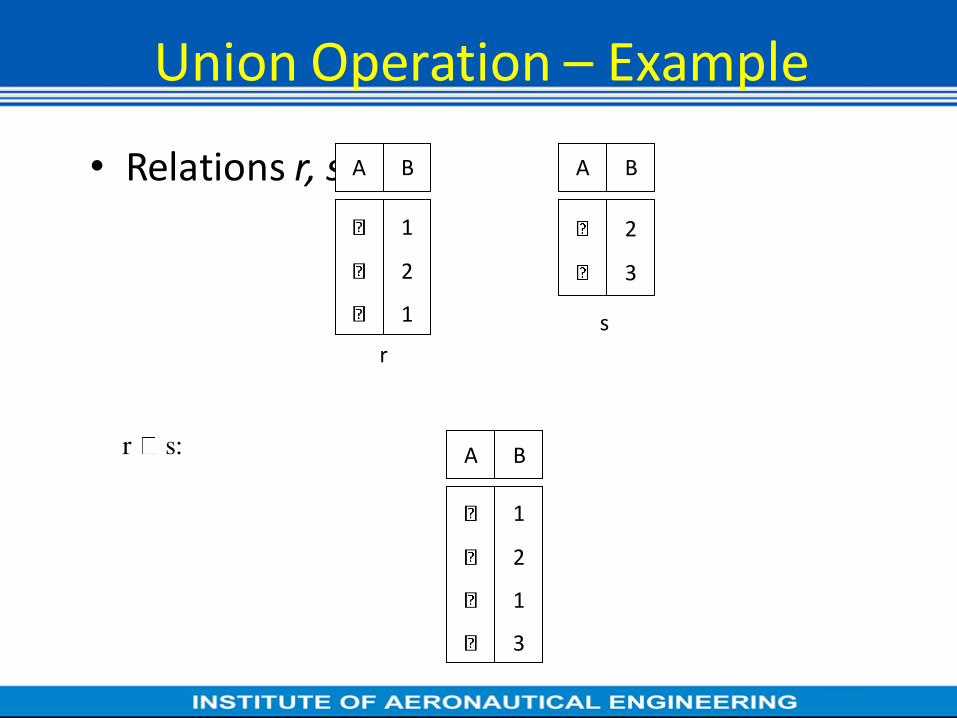
Union Operation – Example
• Relations r, s:
r s:
A B
1
2
1
A B
2
3
r
s
A B
1
2
1
3

Union Operation
• Notation: r s
• Defined as:
r s = {t | t r or t s}
• For r s to be valid.
1. r, s must have the same arity (same number of attributes)
2. The attribute domains must be compatible (e.g., 2nd column
of r deals with the same type of values as does the 2nd
column of s)
• E.g. to find all customers with either an account or a loan
customer-name (depositor) customer-name (borrower)

Set Difference Operation – Example
• Relations r, s:
r – s:
A B
1
2
1
A B
2
3
r
s
A B
1
1

Set Difference Operation
• Notation r – s
• Defined as:
r – s = {t | t r and t s}
• Set differences must be taken between compatible relations.
– r and s must have the same arity
– attribute domains of r and s must be compatible

Cartesian-Product Operation-Example
Relations r, s:
r x s:
A B
1
2
A B
1
1
1
1
2
2
2
2
C D
10
10
20
10
10
10
20
10
E
a
a
b
b
a
a
b
b
C D
10
10
20
10
E
a
a
b
b r
s

Cartesian-Product Operation
• Notation r x s
• Defined as:
r x s = {t q | t r and q s}
• Assume that attributes of r(R) and s(S) are disjoint. (That is,
R S = ).
• If attributes of r(R) and s(S) are not disjoint, then renaming must
be used.

Composition of Operations
• Expressions using multiple operations: Example: A=C(r x s)
• r x s
• A=C(r x s)
A B
1
1
1
1
2
2
2
2
C D
10
10
20
10
10
10
20
10
E
a
a
b
b
a
a
b
b
A B C D E
1
2
2
10
20
20
a
a
b

Rename Operation
• Allows us to name, and therefore to refer to, the results of
relational-algebra expressions.
• Allows us to refer to a relation by more than one name.
Example:
x (E)
returns the expression E under the name X
If a relational-algebra expression E has arity n, then
x (A1, A2, …, An) (E)
returns the result of expression E under the name X, and with
the
attributes renamed to A1, A2, …., An.

RA - Operations Examples
Banking : branch (branch_name, branch_city, assets)
customer (customer_name, customer_street,
customer_city) account (account_number, branch_name, balance) loan (loan_number, branch_name, amount) depositor (customer_name, account_number) borrower (customer_name, loan_number)

• Find all loans of over $1200
Find the loan number for each loan of an amount greater than $1200
amount > 1200 (loan)
loan_number (amount > 1200
(loan))
Find the names of all customers who have a loan, an account, or both, from the bank customer_name (borrower) customer_name (depositor)

Example Queries • Find the names of all customers who have a loan at the Perryridge branch.
Find the names of all customers who have a loan at the Perryridge branch but do
not have an account at any branch of the bank.
customer_name (branch_name =
“Perryridge”
(borrower.loan_number =
loan.loan_number(borrower x loan))) –
customer_name(depositor)
customer_name (branch_name=“Perryridge”
(borrower.loan_number =
loan.loan_number(borrower x loan)))

RA - Advanced Operations - Examples
Find the names of all customers who have a
loan at the Perryridge branch.
customer_name(loan.loan_number = borrower.loan_number ( (branch_name = “Perryridge” (loan)) x borrower))
customer_name (branch_name = “Perryridge” (
borrower.loan_number = loan.loan_number (borrower x loan)))

Outer Join – Example
• Relation loan
Relation borrower
customer_name loan_number
Jones
Smith
Hayes
L-170
L-230
L-155
3000
4000
1700
loan_number amount
L-170
L-230
L-260
branch_name
Downtown
Redwood
Perryridge

Outer Join – Example
• Join
loan borrower
loan_number amount
L-170
L-230
3000
4000
customer_name
Jones
Smith
branch_name
Downtown
Redwood
Jones
Smith
null
loan_number amount
L-170
L-230
L-260
3000
4000
1700
customer_name branch_name
Downtown
Redwood
Perryridge
Left Outer Join
loan borrower

Outer Join – Example
loan_number amount
L-170
L-230
L-155
3000
4000
null
customer_name
Jones
Smith
Hayes
branch_name
Downtown
Redwood
null
loan_number amount
L-170
L-230
L-260
L-155
3000
4000
1700
null
customer_name
Jones
Smith
null
Hayes
branch_name
Downtown
Redwood
Perryridge
null
Full Outer Join
loan borrower
Right Outer Join
loan borrower
Question: can outerjoins be expressed using basic
relational
algebra operations

Division Operation – Example
Relations r, s:
r s: A
B
1
2
A B
1
2
3
1
1
1
3
4
6
1
2
r
s

Another Division Example
A B
a
a
a
a
a
a
a
a
C D
a
a
b
a
b
a
b
b
E
1
1
1
1
3
1
1
1
Relations r, s:
r s:
D
a
b
E
1
1
A B
a
a
C
r
s

Division Operation (Cont.)
• Property
– Let q = r s
– Then q is the largest relation satisfying q x s r
• Definition in terms of the basic algebra operation
Let r(R) and s(S) be relations, and let S R
r s = R-S (r ) – R-S ( ( R-S (r ) x s ) – R-S,S(r ))
To see why
– R-S,S (r) simply reorders attributes of r
– R-S (R-S (r ) x s ) – R-S,S(r) ) gives those tuples t in
R-S (r ) such that for some tuple u s, tu r.

RA - Advanced Operations
• Advanced Operations
– Set intersection
– Natural join
– Aggregation
– Outer Join
– Division
• All above, other than aggregation, can be expressed using basic operations we have seen earlier

Set-Intersection Operation – Example
• Relation r, s:
• r s
A B
1
2
1
A B
2
3
r s
A B
2

Natural Join Operation – Example • Relations r, s:
A B
1
2
4
1
2
C D
a
a
b
a
b
B
1
3
1
2
3
D
a
a
a
b
b
E
r
A B
1
1
1
1
2
C D
a
a
a
a
b
E
s
r s

Notation: r s
Natural-Join Operation
• Let r and s be relations on schemas R and S respectively. Then, r s is a relation on schema R S obtained as follows: – Consider each pair of tuples tr from r and ts from s.
– If tr and ts have the same value on each of the attributes in R S, add a tuple t to the result, where
• t has the same value as tr on r
• t has the same value as ts on s
• Example: R = (A, B, C, D)
S = (E, B, D)
– Result schema = (A, B, C, D, E)
– r s is defined as: r.A, r.B, r.C, r.D, s.E (r.B = s.B r.D = s.D (r x s))

Bank Example Queries • Find the largest account balance
– Strategy:
• Find those balances that are not the largest
– Rename account relation as d so that we can compare
each account balance with all others
• Use set difference to find those account balances
that were not found in the earlier step.
– The query is:
balance(account) - account.balance
(account.balance < d.balance (account x d (account)))

Aggregate Functions and Operations
• Aggregation function takes a collection of values and returns a single value as a result.
avg: average value min: minimum value max: maximum value sum: sum of values count: number of values
• Aggregate operation in relational algebra
E is any relational-algebra expression
– G1, G2 …, Gn is a list of attributes on which to group (can be empty)
– Each Fi is an aggregate function
– Each Ai is an attribute name
)()(,,(),(,,, 221121
Ennn AFAFAFGGG

Aggregate Operation – Example
• Relation r:
A B
C
7
7
3
10
g sum(c) (r) sum(c )
27
Question: Which aggregate operations cannot be expressed using basic relational operations?

Aggregate Operation – Example
• Relation account grouped by branch-name:
branch_name g sum(balance) (account)
branch_name account_number balance
Perryridge
Perryridge
Brighton
Brighton
Redwood
A-102
A-201
A-217
A-215
A-222
400
900
750
750
700
branch_name sum(balance)
Perryridge
Brighton
Redwood
1300
1500
700

Aggregate Functions (Cont.)
• Result of aggregation does not have a name
– Can use rename operation to give it a name
– For convenience, we permit renaming as part of
aggregate operation
branch_name g sum(balance) as sum_balance
(account)

Outer Join
• An extension of the join operation that avoids loss of information.
• Computes the join and then adds tuples form one relation that does
not match tuples in the other relation to the result of the join.
• Uses null values:
– null signifies that the value is unknown or does not exist
– All comparisons involving null are (roughly speaking) false by
definition.
• We shall study precise meaning of comparisons with nulls
later

Outer Join – Example
• Relation loan
Relation borrower
customer_name loan_number
Jones
Smith
Hayes
L-170
L-230
L-155
3000
4000
1700
loan_number amount
L-170
L-230
L-260
branch_name
Downtown
Redwood
Perryridge

Outer Join – Example
• Join
loan borrower
loan_number amount
L-170
L-230
3000
4000
customer_name
Jones
Smith
branch_name
Downtown
Redwood
Jones
Smith
null
loan_number amount
L-170
L-230
L-260
3000
4000
1700
customer_name branch_name
Downtown
Redwood
Perryridge
Left Outer Join
loan borrower

Outer Join – Example
loan_number amount
L-170
L-230
L-155
3000
4000
null
customer_name
Jones
Smith
Hayes
branch_name
Downtown
Redwood
null
loan_number amount
L-170
L-230
L-260
L-155
3000
4000
1700
null
customer_name
Jones
Smith
null
Hayes
branch_name
Downtown
Redwood
Perryridge
null
Full Outer Join
loan borrower
Right Outer Join
loan borrower
Question: can outerjoins be expressed using basic
relational
algebra operations

Null Values
• It is possible for tuples to have a null value, denoted by null, for some
of their attributes
• null signifies an unknown value or that a value does not exist.
• The result of any arithmetic expression involving null is null.
• Aggregate functions simply ignore null values (as in SQL)
• For duplicate elimination and grouping, null is treated like any other
value, and two nulls are assumed to be the same (as in SQL)

Null Values
• Comparisons with null values return the special truth value:
unknown
– If false was used instead of unknown, then not (A < 5)
would not be equivalent to A >= 5
• Three-valued logic using the truth value unknown:
– OR: (unknown or true) = true,
(unknown or false) = unknown
(unknown or unknown) = unknown
– AND: (true and unknown) = unknown,
(false and unknown) = false,
(unknown and unknown) = unknown
– NOT: (not unknown) = unknown
– In SQL “P is unknown” evaluates to true if predicate P

Cont…
– evaluates to unknown
• Result of select predicate is treated as false if it evaluates to
unknown
– NOT: (not unknown) = unknown
– In SQL “P is unknown” evaluates to true if predicate P evaluates
to unknown
• Result of select predicate is treated as false if it evaluates to
unknown

Division Operation
• Notation:
• Suited to queries that include the phrase “for all”.
• Let r and s be relations on schemas R and S respectively where
– R = (A1, …, Am , B1, …, Bn )
– S = (B1, …, Bn)
The result of r s is a relation on schema
R – S = (A1, …, Am)
r s = { t | t R-S (r) u s ( tu r ) }
Where tu means the concatenation of tuples t and u to produce a
single tuple
r
s

Division Operation – Example
Relations r, s:
r s: A
B
1
2
A B
1
2
3
1
1
1
3
4
6
1
2
r
s

Another Division Example
A B
a
a
a
a
a
a
a
a
C D
a
a
b
a
b
a
b
b
E
1
1
1
1
3
1
1
1
Relations r, s:
r s:
D
a
b
E
1
1
A B
a
a
C
r
s

Division Operation (Cont.) • Property
– Let q = r s
– Then q is the largest relation satisfying q x s r
• Definition in terms of the basic algebra operation
Let r(R) and s(S) be relations, and let S R
r s = R-S (r ) – R-S ( ( R-S (r ) x s ) – R-S,S(r ))
To see why
– R-S,S (r) simply reorders attributes of r
– R-S (R-S (r ) x s ) – R-S,S(r) ) gives those tuples t in
R-S (r ) such that for some tuple u s, tu r.

RA - Advanced Operations - Examples
branch (branch_name, branch_city, assets)
customer (customer_name, customer_street, customer_city)
account (account_number, branch_name, balance)
loan (loan_number, branch_name, amount)
depositor (customer_name, account_number)
borrower (customer_name, loan_number)

Example Queries
• Find all loans of over $1200
Find the loan number for each loan of an amount greater than $1200
amount > 1200 (loan)
loan_number (amount > 1200
(loan))
Find the names of all customers who have a loan, an account, or both, from the bank
customer_name (borrower) customer_name (depositor)

Example Queries
• Find the names of all customers who have a loan at the Perryridge branch.
Find the names of all customers who have a loan at the Perryridge branch
but do not have an account at any branch of the bank.
customer_name (branch_name =
“Perryridge”
(borrower.loan_number =
loan.loan_number(borrower x loan))) –
customer_name(depositor)
customer_name (branch_name=“Perryridge”
(borrower.loan_number =
loan.loan_number(borrower x loan)))

Example Queries
• Find the names of all customers who have a loan at the Perryridge branch.
customer_name(loan.loan_number = borrower.loan_number ( (branch_name = “Perryridge” (loan)) x borrower))
customer_name (branch_name = “Perryridge” (
borrower.loan_number = loan.loan_number (borrower x loan)))

Examples of RA Queries
Examples of RA Queries
• person (driver-id, name, address) car (license, year, model)
• accident (report-number, location, date) owns (driver-id, license)
• participated (report-number driver-id, license, damage-amount) employee (person-name, street, city) works (person-name, company-name, salary)
• company (company-name, city) manages (person-name, manager-name) An expressions in the relational algebra:

Examples of RA Queries
a. Find the names of all employees who work for First Bank
Corporation.
• Π person-name (σ company-name = “First Bank Corporation” (works))
b. Find the names and cities of residence of all employees who work
for First Bank Corporation.
• Πperson-name, city (employee ⋈ (σ company-name = “First Bank Corporation” (works)))

c. Find the names, street address, and cities of residence of all employees
who work for First Bank Corporation and earn more than $10,000 per
annum.
• Π person-name, street, city (σ(company-name = “First Bank Corporation” ∧ salary > 10000) works ⋈ employee)
d. Find the names of all employees in this database who live in the same
city as the company for which they work.
• Π person-name (employee ⋈ works ⋈company)
Find the names of all employees who live in the same city and on
the same street as do their managers.
• Π person-name ((employee ⋈ manages) ⋈ (manager-name =
employee2.person-name ∧employee.street = employee2.street ∧employee.city = employee2.city)(ρemployee2 (employee)))

Cont…
e. Find the names of all employees in this database who do not work
for First Bank Corporation.
• Π person-name (σ company-name = “First Bank Corporation”(works)) If people may not work for any company:
Π person-name(employee) - Πperson-name (σ(company-name =
“First Bank Corporation”)(works))
f . Assume the companies may be located in several cities. Find all
companies located in every city in which Small Bank Corporation is
located.
• Π company-name (company ÷ (Πcity (σ company-name = “Small Bank Corporation” (company)))

Examples of RA Queries
• Find the accounts held by more than two customers in the following ways:
a. Using an aggregate function.
• t1 ← account-number 𝒢count customer-name(depositor)
• Π account-number (σ num-holders>2 (ρ account-holders(account-number, num-holders)(t1)))
b. Without using any aggregate functions
• t1 ← (ρd1(depositor) × ρd2 (depositor) × ρd3 (depositor)) • t2 ← σ(d1.account-number=d2.account-number=d3.account-
number)(t1)
Examples of RA Queries
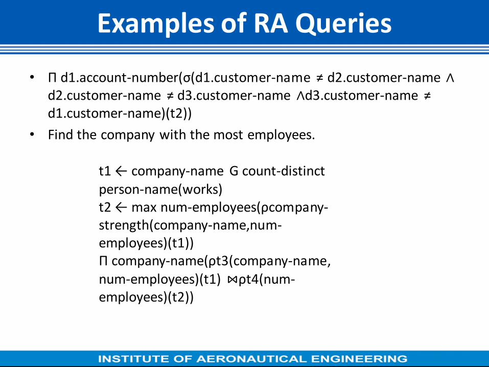
• Π d1.account-number(σ(d1.customer-name ≠ d2.customer-name ∧
d2.customer-name ≠ d3.customer-name ∧d3.customer-name ≠ d1.customer-name)(t2))
• Find the company with the most employees.
t1 ← company-name G count-distinct
person-name(works)
t2 ← max num-employees(ρcompany-
strength(company-name,num-
employees)(t1))
Π company-name(ρt3(company-name,
num-employees)(t1) ⋈ρt4(num-
employees)(t2))

Cont…
b. Find the company with the smallest payroll.
• t1 ← company-name G sum salary(works) t2 ← min payroll(ρcompany-payroll(company-name,payroll)(t1)) Π company-name(ρt3(company-name, payroll)(t1) ⋈ρt4(payroll)(t2))
c. Find those companies whose employees earn a higher salary, on average, than the average salary at First Bank Corporation.
• t1 ← company-nameGsum salary(works) t2 ← min payroll(ρcompany-payroll(company-name,payroll)(t1)) Πcompany-name(ρt3(company-name,payroll)(t1) ⋈ρt4(payroll)(t2))

Tuple Relational Calculus
• A nonprocedural query language, where each query is of the form
{t | P (t ) }
• It is the set of all tuples t such that predicate P is true for t
• t is a tuple variable, t [A ] denotes the value of tuple t on attribute A

Cont.
• t r denotes that tuple t is in relation r
• P is a formula similar to that of the predicate calculus

Predicate Calculus Formula
1. Set of attributes and constants
2. Set of comparison operators: (e.g., , , , , , )
3. Set of connectives: and (), or (v)‚ not ()
4. Implication (): x y, if x if true, then y is true
x y x v y

cont.
5. Set of quantifiers:
t r (Q (t )) ”there exists” a tuple in t in relation r
such that predicate Q (t ) is true
t r (Q (t )) Q is true “for all” tuples t in relation r

Examples of TRC Queries
• branch (branch_name, branch_city, assets )
• customer (customer_name, customer_street,
customer_city )
• account (account_number, branch_name, balance )
• loan (loan_number, branch_name, amount )
• depositor (customer_name, account_number )
• borrower (customer_name, loan_number )

Example Queries
• Find the loan_number, branch_name, and amount for
loans of over $1200
Find the loan number for each loan of an amount greater than
$1200
{t | s loan (t [loan_number ] = s [loan_number ]
s [amount ] 1200)}
Notice that a relation on schema [loan_number ] is implicitly
defined by
the query
{t | t loan t [amount ] 1200}

Example Queries
• Find the names of all customers having a loan, an account, or both
at the bank
{t | s borrower ( t [customer_name ] = s [customer_name ])
u depositor ( t [customer_name ] = u [customer_name ])
• Find the names of all customers who have a loan and an account
at the bank
{t | s borrower ( t [customer_name ] = s [customer_name ])
u depositor ( t [customer_name ] = u [customer_name] )

Example Queries
• Find the names of all customers having a loan at the Perryridge branch
{t | s borrower (t [customer_name ] = s [customer_name ]
u loan (u [branch_name ] = “Perryridge”
u [loan_number ] = s [loan_number ]))}
• Find the names of all customers who have a loan at the
Perryridge branch, but no account at any branch of the bank
{t | s borrower (t [customer_name ] = s [customer_name ]
u loan (u [branch_name ] = “Perryridge”
u [loan_number ] = s [loan_number ]))
not v depositor (v [customer_name ] =
t [customer_name ])}

Example Queries
• Find the names of all customers having a loan from the Perryridge
branch, and the cities in which they live
t | s loan (s [branch_name ] = “Perryridge”
u borrower (u [loan_number ] = s [loan_number ]
t [customer_name ] = u [customer_name ])
v customer (u [customer_name ] = v [customer_name
] t [customer_city ] = v [customer_city ])))}

Example Queries
• Find the names of all customers who have an account at all branches
located in Brooklyn:
t | r customer (t [customer_name ] = r [customer_name ])
( u branch (u [branch_city ] = “Brooklyn”
s depositor (t [customer_name ] = s [customer_name ]
w account ( w[account_number ] = s [account_number ]
( w [branch_name ] = u [branch_name ]))))}

Find the names of all employees who work for First Bank
Corporation:-
i. {t | ∃ s ∈ works (t[person-name] = s[person-name] ∧ s[company-
name] = “First Bank Corporation”)}
ii. { < p > | ∃ c, s (< p, c, s > ∈ works ∧ c = “First Bank Corporation”)}
Cont…

Find the names and cities of residence of all employees who work
for First Bank Corporation:-
i. {t | ∃ r ∈ employee ∃ s ∈ works ( t[person-name] = r[person-
name] ∧ t[city] = r[city] ∧ r[person-name] = s[person-name] ∧ s[company-name] = “First Bank Corporation”)} ii. {< p, c > | ∃ co, sa, st (< p, co, sa > ∈ works ∧ < p, st, c > ∈ employee ∧ co = “First Bank Corporation”)}
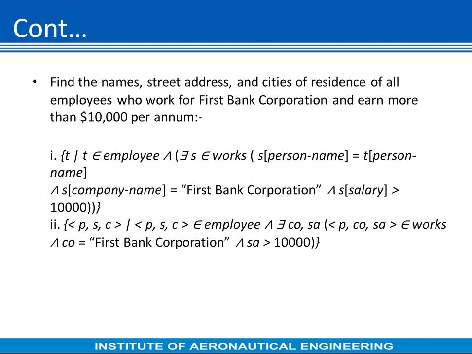
• Find the names, street address, and cities of residence of all
employees who work for First Bank Corporation and earn more
than $10,000 per annum:-
i. {t | t ∈ employee ∧ (∃ s ∈ works ( s[person-name] = t[person-
name] ∧ s[company-name] = “First Bank Corporation” ∧ s[salary] >
10000))}
ii. {< p, s, c > | < p, s, c > ∈ employee ∧ ∃ co, sa (< p, co, sa > ∈ works ∧ co = “First Bank Corporation” ∧ sa > 10000)}
Cont…

Find the names of all employees in this database who live in the same
city
as the company for which they work:-
i. {t | ∃ e ∈ employee ∃ w ∈ works ∃ c ∈ company
(t[person-name] = e[person-name] ∧ e[person-name] = w[person-name] ∧ w[company-name] = c[company-name] ∧ e[city] = c[city])}
Cont…

Domain Relational calculus- Queries
• A nonprocedural query language equivalent in power to the tuple
relational calculus
• Each query is an expression of the form:
{ x1, x2, …, xn | P (x1, x2, …, xn)}
– x1, x2, …, xn represent domain variables
– P represents a formula similar to that of the predicate calculus

Example Queries
• Find the loan_number, branch_name, and amount for loans of over
$1200
{ l, b, a | l, b, a loan a > 1200}
Find the names of all customers who have a loan of over $1200
{ c | l, b, a ( c, l borrower l, b, a loan a > 1200)}
Find the names of all customers who have a loan from the Perryridge
branch and the loan amount
{ c, a | l ( c, l borrower b ( l, b, a loan
b=“Perryridge”))}
{ c, a | l ( c, l borrower l, “ Perryridge”, a loan)}

Example Queries
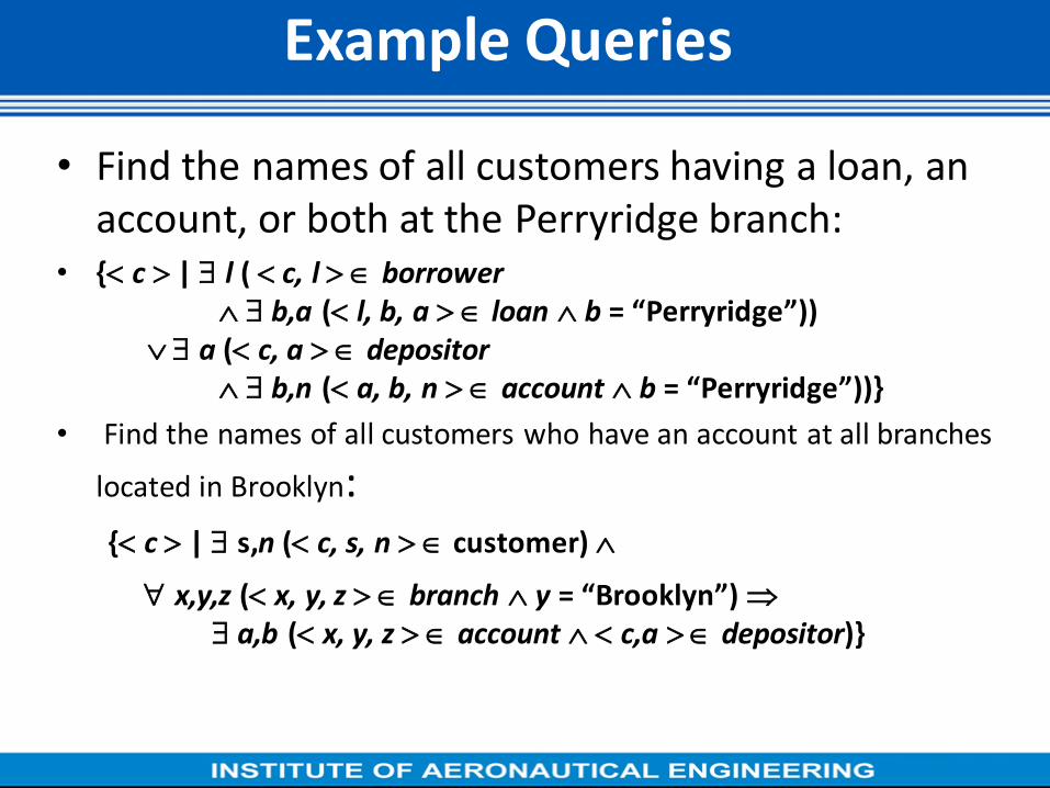
• Find the names of all customers having a loan, an account, or both at the Perryridge branch:
{ c | s,n ( c, s, n customer)
x,y,z ( x, y, z branch y = “Brooklyn”)
a,b ( x, y, z account c,a depositor)}
Find the names of all customers who have an account at all branches
located in Brooklyn:
{ c | l ( c, l borrower
b,a ( l, b, a loan b = “Perryridge”)) a ( c, a depositor
b,n ( a, b, n account b = “Perryridge”))}

Safety of Expressions
The expression:
{ x1, x2, …, xn | P (x1, x2, …, xn )}
is safe if all of the following hold:
1. All values that appear in tuples of the expression are values from
dom (P ) (that is, the values appear either in P or in a tuple of a
relation mentioned in P ).
2. For every “there exists” subformula of the form x (P1(x )), the
subformula is true if and only if there is a value of x in dom (P1)
such that P1(x ) is true.
3. For every “for all” subformula of the form x (P1 (x )), the subformula is
true if and only if P1(x ) is true for all values x from dom (P1).

Domain Relational calculus- Queries
• A nonprocedural query language equivalent in power to the tuple
relational calculus
• Each query is an expression of the form:
{ x1, x2, …, xn | P (x1, x2, …, xn)}
– x1, x2, …, xn represent domain variables
– P represents a formula similar to that of the predicate calculus

Example Queries
• Find the loan_number, branch_name, and amount for loans of over
$1200
Find the names of all customers who have a loan from the Perryridge branch and the loan amount:
{ c, a | l ( c, l borrower b ( l, b, a
loan b=“Perryridge”))}
{ c, a | l ( c, l borrower l, “ Perryridge”, a loan)}
{ c | l, b, a ( c, l borrower l, b, a loan a > 1200)}
Find the names of all customers who have a loan of over $1200
{ l, b, a | l, b, a loan a > 1200}
Example Queries
• Find the names of all customers having a loan, an
account, or both at the Perryridge branch: • { c | l ( c, l borrower
b,a ( l, b, a loan b = “Perryridge”)) a ( c, a depositor
b,n ( a, b, n account b = “Perryridge”))}
• Find the names of all customers who have an account at all branches
located in Brooklyn:
{ c | s,n ( c, s, n customer)
x,y,z ( x, y, z branch y = “Brooklyn”)
a,b ( x, y, z account c,a depositor)}

Safety of Expressions
The expression:
{ x1, x2, …, xn | P (x1, x2, …, xn )}
is safe if all of the following hold:
1. All values that appear in tuples of the expression are values from
dom (P ) (that is, the values appear either in P or in a tuple of a
relation mentioned in P ).
2. For every “there exists” subformula of the form x (P1(x )), the
subformula is true if and only if there is a value of x in dom (P1)
such that P1(x ) is true.
3. For every “for all” subformula of the form x (P1 (x )), the subformula is
true if and only if P1(x ) is true for all values x from dom (P1).

Expressive Power of Algebra and Calculus
Unsafe query: • z a syntactically correct calculus query that has an infinite
number of answers
• E.g., { S | ¬ ( S ∈ Sailors ) }
• Every query that can be expressed in relational algebra can be expressed as a safe query in DRC / TRC; the converse is also true
• Relational Completeness
• Query language (e.g., SQL) can express every query that is expressible in relational algebra
• In addition, commercial query languages can express some queries that cannot be expressed
• in relational algebra

UNIT - III
BASIC SQL QUERY

• SQL can execute queries against a database
• SQL can retrieve data from a database
• SQL can insert records in a database
• SQL can update records in a database
• SQL can delete records from a database
• SQL can create new databases
• SQL can create new tables in a database
• SQL can create stored procedures in a database
• SQL can create views in a database
• SQL can set permissions on tables, procedures, and views
• Although SQL is an ANSI (American National Standards Institute) standard,
there are different versions of the SQL language.
SQL

• Data definition statement are use to define the
database structure or table.
• Statement Description CREATE Create new
database/table.
• ALTER: Modifies the structure of database/table.
• DROP : Deletes a database/table.
• TRUNCATE: Remove all table records including
allocated table spaces.
• RENAME: Rename the database/table.
Data Definition Language (DDL)

Allows the specification of not only a set of relations but also
information about each relation, including:
• The schema for each relation.
• The domain of values associated with each attribute.
• Integrity constraints
• The set of indices to be maintained for each relations.
• Security and authorization information for each relation.
• The physical storage structure of each relation on disk.
Data Definition Language

Domain Types in SQL
• char(n):Fixed length character string, with user-specified length n.
• varchar(n): Variable length character strings, with user-specified maximum length n.
• Int: Integer (a finite subset of the integers that is machine- dependent).
• Smallint: Small integer (a machine-dependent subset of the integer domain type).
• numeric(p,d): Fixed point number, with user-specified precision of
• p digits, with n digits to the right of decimal point.
• real, double precision: Floating point and double-precision floating point numbers, with machine-dependent precision.
• float(n):Floating point number, with user-specified precision of at least n digits.

An SQL relation is defined using the create table command:
• create table r (A1 D1, A2 D2, ..., An Dn,
• (integrity-constraint1),
• ...,
• (integrity-constraintk))
• r is the name of the relation
• each Ai is an attribute name in the schema of relation r
• Di is the data type of values in the domain of attribute Ai
• Example:
• create table branch
• (branch_name char(15) not null,
• branch_city char(30),
• assets integer)
Create Table Construct
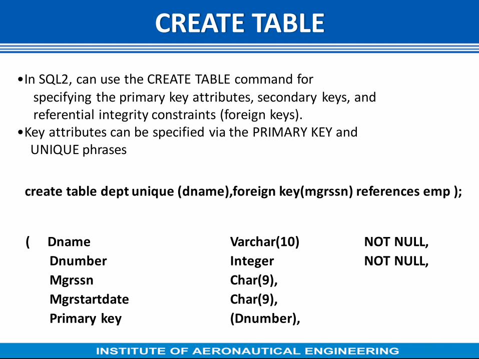
CREATE TABLE
•In SQL2, can use the CREATE TABLE command for
specifying the primary key attributes, secondary keys, and
referential integrity constraints (foreign keys).
•Key attributes can be specified via the PRIMARY KEY and
UNIQUE phrases
( Dname Varchar(10) NOT NULL,
Dnumber Integer NOT NULL,
Mgrssn Char(9),
Mgrstartdate Char(9),
Primary key (Dnumber),
create table dept unique (dname),foreign key(mgrssn) references emp );

– not null
– primary key (A1, ..., An )
• Example:Declare branch_name as the primary key for
branch and ensure that the values of assets are non-
negative.
• create table branch (branch_name char(15), branch_city
char(30), Assets integer, primary key(branch_name))
• primary key declaration on an attribute automatically
ensures not null in SQL- 92 onwards, needs to be
explicitly stated in SQL-89
Integrity Constraints in Create Table

DROP TABLE
– Used to remove a relation (base table) and its definition
– The relation can no longer be used in queries, updates, or any other commands since its description no longer exists
– Example:
• DROP TABLE DEPENDENT;
Drop and Alter Table Constructs:
• The drop table command deletes all information about the dropped relation from the database.
• The alter table command is used to add attributes to an existing relation: alter table r add A D
• where A is the name of the attribute to be added to relation r and D is the domain of A.
– All tuples in the relation are assigned null as the value for the new attribute.
• The alter table command can also be used to drop attributes of a relation: alter table r drop A
• where A is the name of an attribute of relation r
– Dropping of attributes not supported by many databases

ALTER TABLE • Used to add an attribute to one of the base relations
• The new attribute will have NULLs in all the tuples of the relation right after
the command is executed; hence, the NOT NULL constraint is not allowed
for such an attribute
Example:
• ALTER TABLE EMPLOYEE ADD JOB VARCHAR(12);
• The database users must still enter a value for the new attribute JOB for
each EMPLOYEE tuple. This can be done using the UPDATE command.
Integrity Constraints
– Integrity constraints guard against accidental damage to the database,
by ensuring that authorized changes to the database do not result in a
loss of data consistency.
• A checking account must have a balance greater than $10,000.00
• A salary of a bank employee must be at least $4.00 an hour
• A customer must have a (non-null) phone number

Constraints on a Single Relation
• not null
• primary key
• unique
• check (P ), where P is a predicate
Not Null Constraint:
• Declare branch_name for branch is not null
• branch_name char(15) not null
• Declare the domain Dollars to be not null
• create domain Dollars numeric(12,2) not null

The Unique Constraint
– unique ( A1, A2, …, Am)
• The unique specification states that the attributes
A1, A2, … Am Form a candidate key.
• Candidate keys are permitted to be null (in contrast to primary keys).
The check clause – check (P ), where P is a predicate
• Declare branch_name as the primary key for branch and ensure that the
values of assets are non-negative.
• create table branch (branch_name char(15), branch_city char(30),
Assets integer, primary key(branch_name), CHECK (assets >= 0))

• The check clause permits domains to be restricted:
• Use check clause to ensure that an hourly _ wage domain allows
only values greater than a specified value.
• create domain hourly_ wage numeric (5,2) constraint value _ test
check(value > = 4.00)
• The domain has a constraint that ensures that the hourly _ wage is
greater than 4.00
• The clause constraint value _ test is optional; useful to indicate
which constraint an update violated

Referential Integrity
■Ensures that a value that appears in one relation for a given set of
attributes also appears for a set of attributes in another relation.
Example:If “Perryridge” is a branch name appearing in one of the tuples in the account relation, then there exists a tuple in the
branch relation for branch “Perryridge”. ■Primary and candidate keys and foreign keys can be specified as part
of the SQL create table statement:
■The primary key clause lists primary key (PK) attributes.
■The unique key clause lists candidate key attributes
■The foreign key clause lists foreign key (FK) attributes and the
name of the relation referenced by the FK. By default, a FK
references PK attributes of the referenced table.

Referential Integrity in SQL – Example
• create table customer (customer_name char(20), customer_street
char(30), customer_city char(30), primary key (customer_name ));
• create table branch (branch_name char(15), branch_city char(30), assets
numeric(12,2), primary key(branch_name ));
• create table account (account_number char(10), branch_name char(15),
balance integer,primary key(account_number),foreign key(branch_name)
references branch );
• create table depositor (customer_name char(20), account_number
char(10),primary key (customer_name, account_number),foreign key
(account_number ) references account,foreign key (customer_name )
references customer );

TRUNCATE TABLE Statement
This SQL tutorial explains how to use the SQL TRUNCATE TABLE
statement with syntax and examples.
• Description:The SQL TRUNCATE TABLE statement is used to remove
all records from a table. It performs the same function as a DELETE
statement without a WHERE clause.
Syntax
The syntax for the TRUNCATE TABLE statement in SQL is:
TRUNCATE TABLE table_name;

The SQL DROP TABLE Statement
• The DROP TABLE statement is used to drop an existing table in a
database.
Syntax
DROP TABLE table_name;
• Be careful before dropping a table. Deleting a table will result in loss
of complete information stored in the table!

Assertions • An assertion is a predicate expressing a condition that we wish the
database always to satisfy.
An assertion in SQL takes the form
• create assertion <assertion-name> check <predicate>
When an assertion is made, the system tests it for validity, and tests
it again on every update that may violate the assertion
– This testing may introduce a significant amount of overhead;
hence assertions should be used with great care.
• Asserting for all X, P(X) is achieved in a round-about fashion using
not exists X such that not P(X)

Using General Assertions
• Specify a query that violates the condition; include inside a NOT EXISTS
clause
• Query result must be empty
– if the query result is not empty, the assertion has been violated
Assertion Example
– Every loan has at least one borrower who maintains an account with a
minimum balance or $1000.00
• create assertion balance_constraint check (not exists (select * from loan
where not exists (select * from borrower, depositor, account
whereloan.loan_number = borrower.loan_number and
borrower.customer_name = depositor.customer_name and
depositor.account_number = account.account_number and
account.balance >= 1000)));

Example-2 • The sum of all loan amounts for each branch must be less than the sum of all
account balances at the branch.
• create assertion sum_constraint check (not exists (select * from branch where (select sum(amount ) from loan where loan.branch_name = branch.branch_name )>= (select sum(amount )
from account where loan.branch_name = branch.branch_name )));
Assertions: Another Example
• “The salary of an employee must not be greater than the salary of the manager of the department that the employee works for’’
• Creat assertion salary_constraint check (not exists
(Select * from employee e, employee m, department d where e.Salary > m.Salary and e.Dno=d.Number and d.Mgrssn=m.Ssn));

SQL Triggers
– Objective: to monitor a database and take action when a condition occurs
– Triggers are expressed in a syntax similar to assertions and include the following:
• event (e.g., an update operation)
• condition
• action (to be taken when the condition is satisfied)
SQL Triggers: An Example
A trigger to compare an employee’s salary to his/her supervisor during insert or update operations:
Create Trigger Inform_supervisor Before Insert Or Update Of
Salary, Supervisor _ ssn On Employee For Each Row When (New.Salary >(Select Salary From Employee Where Ssn=new.Supervisor _ ssn)) Inform_supervisor (new.supervisor_ssn,new.ssn);

SELECT Statement
Syntax
SELECT column-names FROM table-name;
• The SELECT statement retrieves data from a database.
• The data is returned in a table-like structure called a result-set.
• SELECT is the most frequently used action on a database.
To select all columns use *
SELECT * FROM table-name;

WHERE Clause
• To limit the number of rows use the WHERE clause.
• The WHERE clause filters for rows that meet certain criteria.
• WHERE is followed by a condition that returns either true or false.
• WHERE is used with SELECT, UPDATE, and DELETE.
A WHERE clause with an UPDATE statement:
UPDATE table-name SET column-name = value WHERE condition
A WHERE clause with a DELETE statement: DELETE table-name
WHERE condition

INSERT Into With Select Example
The Bigfoot Brewery supplier is also a customer.
Add a customer record with values from the supplier table
• INSERT INTO Customer (FirstName, LastName, City, Country, Phone)
SELECT LEFT(ContactName, CHARINDEX(' ',ContactName) -1),
SUBSTRING(ContactName, CHARINDEX(' ',ContactName) + 1, 100),
City, Country, Phone FROM Supplier WHERE CompanyName = 'Bigfoot
Breweries‘;

UPDATE Statement
• The UPDATE statement updates data values in a database.
• UPDATE can update one or more records in a table.
• Use the WHERE clause to UPDATE only specific records.
• The general syntax is:
UPDATE table-name SET column-name = value, column-name = value, ...
• To limit the number of records to UPDATE append a WHERE clause:
UPDATE table-name SET column-name = value, column-name = value, ...
WHERE condition
• UPDATE Examples
Problem: discontinue all products in the database UPDATE Product SET Is
Discontinued = 1
• UPDATE Product SET IsDiscontinued = 1 WHERE UnitPrice > 50

DELETE Statement
• DELETE permanently removes records from a table.
• DELETE can delete one or more records in a table.
• Use the WHERE clause to DELETE only specific records.
• The general syntax is:
DELETE table-name ;
To delete specific records append a WHERE clause: DELETE table-
name WHERE condition;
SQL DELETE Examples
• Problem: Delete all products.
DELETE Product;
• Problem: Delete products over $50.
DELETE Product WHERE UnitPrice > 50;

Integrity and Security
• Domain Constraints
• Referential Integrity
• Assertions
• Triggers
• Security
• Authorization
• Authorization in SQL

Domain Constraints • Integrity constraints guard against accidental damage to the
database, by ensuring that authorized changes to the database do
not result in a loss of data consistency.
• Domain constraints are the most elementary form of integrity
constraint.
• They test values inserted in the database, and test queries to
ensure that the comparisons make sense.
• New domains can be created from existing data types
E.g. create domain Dollars numeric(12, 2)
create domain Pounds numeric(12,2)
• We cannot assign or compare a value of type Dollars to a value of
type Pounds.
However, we can convert type as below
(cast r.A as Pounds)
(Should also multiply by the dollar-to-pound conversion-rate)

Domain Constraints (Cont.)
• The check clause in SQL-92 permits domains to be restricted:
- Use check clause to ensure that an hourly-wage domain allows
only values greater than a specified value.
create domain hourly-wage numeric(5,2)
constraint value-test check(value > = 4.00)
- The domain has a constraint that ensures that the hourly-wage is
greater than 4.00
- The clause constraint value-test is optional; useful to indicate
which constraint an update violated.
• Can have complex conditions in domain check
- create domain AccountType char(10)
constraint account-type-test
check (value in (‘Checking’, ‘Saving’)) - - check (branch-name in (select branch-name from branch))

Referential Integrity
• Ensures that a value that appears in one relation for a given set of
attributes also appears for a certain set of attributes in another relation.
Example: If “Perryridge” is a branch name appearing in one of the tuples
in the account relation, then there exists a tuple in the branch relation for
branch “Perryridge”. • Formal Definition
Let r1(R1) and r2(R2) be relations with primary keys K1 and K2
respectively.
The subset α of R2 is a foreign key referencing K1 in relation r1,
if for every t2 in r2 there must be a tuple t1 in r1 such that
t1[K1] = t2[α]. Referential integrity constraint also called subset dependency since its can
be written as
Πα (r2) ⊆ ΠK1 (r1)

Referential Integrity in the E-R Model
• Consider relationship set R between entity sets E1 and E2. The
relational schema for R includes the primary keys K1 of E1 and K2 of
E2.
- Then K1 and K2 form foreign keys on the relational
schemas for E1 and E2 respectively.
• Weak entity sets are also a source of referential integrity constraints.
- For the relation schema for a weak entity set must include the
primary key attributes of the entity set on which it depends

Checking Referential Integrity on Database Modification
• The following tests must be made in order to preserve the
following referential integrity constraint:
Πα (r2) ⊆ ΠK (r1)
• Insert. If a tuple t2 is inserted into r2, the system must ensure
that there is a tuple t1 in r1 such that t1[K] = t2[α]. That is
t2 [α] ∈ ΠK (r1)
• Delete. If a tuple, t1 is deleted from r1, the system must
compute the set of tuples in r2 that reference t1:
σα = t1[K] (r2)
-If this set is not empty
- either the delete command is rejected as an error, or
- the tuples that reference t1 must themselves be deleted
(cascading deletions are possible).

Database Modification (Cont.)
• Update. There are two cases:
If a tuple t2 is updated in relation r2 and the update modifies values
for foreign key α, then a test similar to the insert case is made: Let t2’ denote the new value of tuple t2. The system must ensure
that t2’[α] ∈ ΠK(r1)
If a tuple t1 is updated in r1, and the update modifies values for the
primary key (K), then a test similar to the delete case is made:
1. The system must compute σα = t1[K] (r2)
using the old value of t1 (the value before the update is applied).
2. If this set is not empty
1. the update may be rejected as an error, or
2. the update may be cascaded to the tuples in the set, or
3. the tuples in the set may be deleted.

Referential Integrity in SQL
Primary and candidate keys and foreign keys can be specified as part of
the SQL create table statement:
The primary key clause lists attributes that comprise the primary key.
The unique key clause lists attributes that comprise a candidate key.
The foreign key clause lists the attributes that comprise the foreign key
and the name of the relation referenced by the foreign key.
By default, a foreign key references the primary key attributes of the
referenced table foreign key (account-number) references account
Short form for specifying a single column as foreign key
account-number char (10) references account
Reference columns in the referenced table can be explicitly specified
but must be declared as primary/candidate keys
foreign key (account-number) references account(account-number)

Referential Integrity in SQL – Example
create table customer
(customer-name char(20),
customer-street char(30),
customer-city char(30),
primary key (customer-name))
create table branch
(branch-name char(15),
branch-city char(30),
assets integer,
primary key (branch-name))

Referential Integrity in SQL- Example (Cont.)
create table account
(account-number char(10), branch-name char(15),
balance integer, primary key (account-number),
foreign key (branch-name) references branch)
create table depositor
(customer-name char(20), account-number char(10),
primary key (customer-name, account-number),
foreign key (account-number) references account,
foreign key (customer-name) references customer)

Cascading Actions in SQL
create table account
. . .
foreign key(branch-name) references branch
on delete cascade
on update cascade
. . . )
Due to the on delete cascade clauses, if a delete of a tuple in
branch results in referential-integrity constraint violation, the
delete “cascades” to the account relation, deleting the tuple that
refers to the branch that was deleted
Cascading updates are similar.

Cascading Actions in SQL (Cont.) • If there is a chain of foreign-key dependencies across multiple
relations, with on delete cascade specified for each dependency,
a deletion or update at one end of the chain can propagate across
the entire chain.
• If a cascading update to delete causes a constraint violation that
cannot be handled by a further cascading operation, the system
aborts the transaction.
- As a result, all the changes caused by the transaction and its
cascading actions are undone.

• Referential integrity is only checked at the end of a transaction
Intermediate steps are allowed to violate referential integrity
provided later steps remove the violation . Otherwise it would be
impossible to create some database states, e.g. insert two tuples
whose foreign keys point to each other
# E.g. spouse attribute of relation
marriedperson(name, address, spouse)
(Cont.)

Referential Integrity in SQL (Cont.)
• Alternative to cascading:
on delete set null
on delete set default
• Null values in foreign key attributes complicate SQL referential
integrity semantics, and are best prevented using not null
-if any attribute of a foreign key is null, the tuple is defined to satisfy
the foreign key constraint!

Assertions
• An assertion is a predicate expressing a condition that we wish
the database always to satisfy.
• An assertion in SQL takes the form
create assertion <assertion-name> check <predicate>
• When an assertion is made, the system tests it for validity, and
tests it again on every update that may violate the assertion
- This testing may introduce a significant amount of overhead;
hence assertions should be used with great care.
• Asserting
for all X, P(X)
is achieved in a round-about fashion using
not exists X such that not P(X)

Assertion Example
• The sum of all loan amounts for each branch must be less than
the sum of all account balances at the branch.
create assertion sum-constraint check
(not exists (select * from branch
where (select sum(amount) from loan
where loan.branch-name
branch.branch-name)>= (select sum(amount) from account where
loan.branch-name =
branch.branch-name)));

Assertion Example
• Every loan has at least one borrower who maintains an account with a
minimum balance or $1000.00
create assertion balance-constraint check
(not exists ( select * from loan where not exists
(select * from borrower, depositor, account
where loan.loan-number = borrower.loan-number
and borrower.customer-name =
depositor.customer- name and depositor.account-
number = account.account-number and
account.balance >= 1000)));

Triggers • A trigger is a statement that is executed automatically by the
system as a side effect of a modification to the database.
• To design a trigger mechanism, we must:
Specify the conditions under which the trigger is to be
executed.
Specify the actions to be taken when the trigger executes.
• Triggers introduced to SQL standard in SQL:1999, but supported even earlier
using non-standard syntax by most databases.

Trigger Example
• Suppose that instead of allowing negative account balances, the
bank deals with overdrafts by
setting the account balance to zero
creating a loan in the amount of the overdraft
giving this loan a loan number identical to the
account number of the overdrawn account
• The condition for executing the trigger is an update to the account
relation that results in a negative balance value.

Trigger Example in SQL:1999 create trigger overdraft-trigger after update on account
referencing new row as nrow
for each row
when nrow.balance < 0
begin atomic
insert into borrower
(select customer-name, account-number
from depositor
where nrow.account-number =depositor.account-number);
insert into loan values(n.row.account-number,
nrow.branch-name, – nrow.balance);
update account set balance = 0
where account.account-number = nrow.account-number
end

Triggering Events and Actions in SQL
• Triggering event can be insert, delete or update
• Triggers on update can be restricted to specific attributes
E.g. create trigger overdraft-trigger after update of balance on
account
• Values of attributes before and after an update can be referenced
referencing old row as : for deletes and updates
referencing new row as : for inserts and updates
• Triggers can be activated before an event, which can serve as extra
constraints. E.g. convert blanks to null.
create trigger setnull-trigger before update on r
referencing new row as nrow
for each row when nrow.phone-number = ‘ ‘ set nrow.phone-number = null

External World Actions • ! We sometimes require external world actions to be triggered on a
• database update
• " E.g. re-ordering an item whose quantity in a warehouse has become
• small, or turning on an alarm light,
• ! Triggers cannot be used to directly implement external-world
• actions, BUT
• " Triggers can be used to record actions-to-be-taken in a separate table
• " Have an external process that repeatedly scans the table, carries out
• external-world actions and deletes action from table
• ! E.g. Suppose a warehouse has the following tables
• " inventory(item, level): How much of each item is in the warehouse
• " minlevel(item, level) : What is the minimum desired level of each item
• " reorder(item, amount): What quantity should we re-order at a time
• " orders(item, amount) : Orders to be placed (read by external process)

Statement Level Triggers
• Instead of executing a separate action for each affected row, a
single action can be executed for all rows affected by a transaction
- Use for each statement instead of for each row
- Use referencing old table or referencing new table to refer to
temporary tables (called transition tables) containing the affected
rows
• Can be more efficient when dealing with SQL statements that
update a large number of rows

External World Actions
• We sometimes require external world actions to be triggered on a
database update
- E.g. re-ordering an item whose quantity in a warehouse has
become small, or turning on an alarm light,
• Triggers cannot be used to directly implement external-world
actions, BUT
- Triggers can be used to record actions-to-be-taken in a separate table
- Have an external process that repeatedly scans the table, carries out
external-world actions and deletes action from table
• E.g. Suppose a warehouse has the following tables
- inventory(item, level): How much of each item is in the warehouse
- minlevel(item, level) : What is the minimum desired level of each item
- reorder(item, amount): What quantity should we re-order at a time
- orders(item, amount) : Orders to be placed (read by external process)

External World Actions (Cont.) • create trigger reorder-trigger after update of amount on inventory
referencing old row as orow, new row as nrow
for each row
when nrow.level < = (select level
from minlevel
where minlevel.item = orow.item)
and orow.level > (select level from minlevel
where minlevel.item = orow.item)
begin
insert into orders
(select item, amount
from reorder
where reorder.item = orow.item)
end

Triggers in MS-SQLServer Syntax
• create trigger overdraft-trigger on account
for update as if inserted.balance < 0
begin
insert into borrower (select customer-name,account-number
from depositor, inserted
where inserted.account-number = depositor.account-number)
insert into loan values
(inserted.account-number, inserted.branch-name,
– inserted.balance)
update account set balance = 0
from account, inserted
where account.account-number = inserted.account-number
end

When Not To Use Triggers
• Triggers were used earlier for tasks such as
maintaining summary data (e.g. total salary of each department)
• Replicating databases by recording changes to special relations
(called change or delta relations) and having a separate process
that applies the changes over to a replica
• There are better ways of doing these now:
- Databases today provide built in materialized view facilities to
maintain summary data
- Databases provide built-in support for replication
• Encapsulation facilities can be used instead of triggers in many cases
- Define methods to update fields
- Carry out actions as part of the update methods instead of
through a trigger

Security
• Security - protection from malicious attempts to steal or modify data.
Database system level
- Authentication and authorization mechanisms to allow
specific users access only to required data
- We concentrate on authorization in the rest of this chapter
Operating system level
- Operating system super-users can do anything they want
to the database! Good operating system level security is
required.
Network level: must use encryption to prevent
- Eavesdropping (unauthorized reading of messages)
- Masquerading (pretending to be an authorized user or sending
messages supposedly from authorized users)

Security (Cont.)
Physical level
- Physical access to computers allows destruction of
data by intruders; traditional lock-and-key security
is needed
- Computers must also be protected from floods, fire,
etc.
Human level
- Users must be screened to ensure that an authorized
users do not give access to intruders
- Users should be trained on password selection and
secrecy

Authorization
• Forms of authorization on parts of the database:
Read authorization - allows reading, but not modification of data.
Insert authorization - allows insertion of new data, but not
modification of existing data.
Update authorization - allows modification, but not deletion of data.
Delete authorization - allows deletion of data
Forms of authorization to modify the database schema:
Index authorization - allows creation and deletion of indices.
Resources authorization - allows creation of new relations.
Alteration authorization - allows addition or deletion of attributes in a
relation.
Drop authorization - allows deletion of relations.

Authorization and Views
Users can be given authorization on views, without being given any
authorization on the relations used in the view definition
Ability of views to hide data serves both to simplify usage of the
system and to enhance security by allowing users access only to
data they need for their job
A combination or relational-level security and view-level security
can be used to limit a user’s access to precisely the data that user needs.

View Example
Suppose a bank clerk needs to know the names of the customers of
each branch, but is not authorized to see specific loan information.
- Approach: Deny direct access to the loan relation, but grant access
to the view cust-loan, which consists only of the names of
customers and the branches at which they have a loan.
- The cust-loan view is defined in SQL as follows:
create view cust-loan as
select branchname, customer-name
from borrower, loan
where borrower.loan-number = loan.loan-number

View Example (Cont.)
The clerk is authorized to see the result of the query:
select *from cust-loan
When the query processor translates the result into a query on the
actual relations in the database, we obtain a query on borrower
and loan.
Authorization must be checked on the clerk’s query before query processing replaces a view by the definition of the view.
Authorization on Views
Creation of view does not require resources authorization since
no real relation is being created
The creator of a view gets only those privileges that provide no
additional authorization beyond that he already had.
E.g. if creator of view cust-loan had only read authorization on
borrower and loan, he gets only read authorization on cust-loan

Granting of Privileges The passage of authorization from one user to another may be
represented by an authorization graph.
The nodes of this graph are the users.
The root of the graph is the database administrator.
Consider graph for update authorization on loan.
An edge Ui →Uj indicates that user Ui has granted update
authorization on loan to Uj.

Authorization Grant Graph
Requirement: All edges in an authorization graph must be part of
some path originating with the database administrator
If DBA revokes grant from U1:
- Grant must be revoked from U4 since U1 no longer has authorization
- Grant must not be revoked from U5 since U5 has another
authorization path from DBA through U2
Must prevent cycles of grants with no path from the root:
- DBA grants authorization to U7
- U7 grants authorization to U8
- U8 grants authorization to U7
- DBA revokes authorization from U7
Must revoke grant U7 to U8 and from U8 to U7 since there is no
path from DBA to U7 or to U8 anymore.

Security Specification in SQL
The grant statement is used to confer authorization
grant <privilege list>
on <relation name or view name> to <user list>
<user list> is:
- a user-id
- public, which allows all valid users the privilege granted
- A role (more on this later)
Granting a privilege on a view does not imply granting any
privileges on the underlying relations.
The grantor of the privilege must already hold the privilege on the
specified item (or be the database administrator).

Privileges in SQL
select: allows read access to relation,or the ability to query using
the view
- Example: grant users U1, U2, and U3 select authorization on the
branch relation:
grant select on branch to U1, U2, U3
insert: the ability to insert tuples
update: the ability to update using the SQL update statement
delete: the ability to delete tuples.
references: ability to declare foreign keys when creating relations.
usage: In SQL-92; authorizes a user to use a specified domain
all privileges: used as a short form for all the allowable privileges

Privilege To Grant Privileges
with grant option: allows a user who is granted a privilege to
pass the privilege on to other users.
- Example:
grant select on branch to U1 with grant option
gives U1 the select privileges on branch and allows U1 to grant this
privilege to others

Roles Roles permit common privileges for a class of users can be
specified just once by creating a corresponding “role”
Privileges can be granted to or revoked from roles, just like user
Roles can be assigned to users, and even to other roles
SQL:1999 supports roles
create role teller
create role manager
grant select on branch to teller
grant update (balance) on account to teller
grant all privileges on account to manager
grant teller to manager
grant teller to alice, bob
grant manager to avi

Revoking Authorization in SQL
The revoke statement is used to revoke authorization.
revoke<privilege list>
on <relation name or view name> from <user list>
[restrict|cascade]
Example:
revoke select on branch from U1, U2, U3 cascade
Revocation of a privilege from a user may cause other users also to
lose that privilege; referred to as cascading of the revoke.
We can prevent cascading by specifying restrict:
revoke select on branch from U1, U2, U3 restrict
With restrict, the revoke command fails if cascading revokesare
required.

Revoking Authorization in SQL (Cont.)
<privilege-list> may be all to revoke all privileges the revokee may
hold.
If <revokee-list> includes public all users lose the privilege except
those granted it explicitly.
If the same privilege was granted twice to the same user by different
grantees, the user may retain the privilege after the revocation.
All privileges that depend on the privilege being revoked are also
revoked.

Limitations of SQL Authorization SQL does not support authorization at a tuple level
- E.g. we cannot restrict students to see only (the tuples storing)
their own grades
With the growth in Web access to databases, database accesses
come primarily from application servers.
- End users don't have database user ids, they are all mapped
to the same database user id
All end-users of an application (such as a web application) may be
mapped to a single database user

The task of authorization in above cases falls on the application
program, with no support from SQL
- Benefit: fine grained authorizations, such as to individual tuples, can
be implemented by the application.
- Drawback: Authorization must be done in application code, and may
be dispersed all over an application
Checking for absence of authorization loopholes becomes very difficult
since it requires reading large amounts of application code

Joins and Views

Joined Relations
• Join operations take two relations and return as a result another relation.
• These additional operations are typically used as subquery expressions in the from clause
• Join condition – defines which tuples in the two relations match, and what attributes are present in the result of the join.
• Join type – defines how tuples in each relation that do not match any tuple in the other relation (based on the join condition) are treated.
Join Types
inner join
left outer join
right outer join
full outer join
Join Conditions
natural
on <predicate> using (A1, A2, ..., An)

Join - Examples
• Relation loan
customer-name loan-number
Jones
Smith
Hayes
L-170
L-230
L-155
amount
3000
4000
1700
branch-name
Downtown
Redwood
Perryridge
loan-number
L-170
L-230
L-260
Relation borrower
Note: borrower information missing for L-260 and loan information missing for L-155
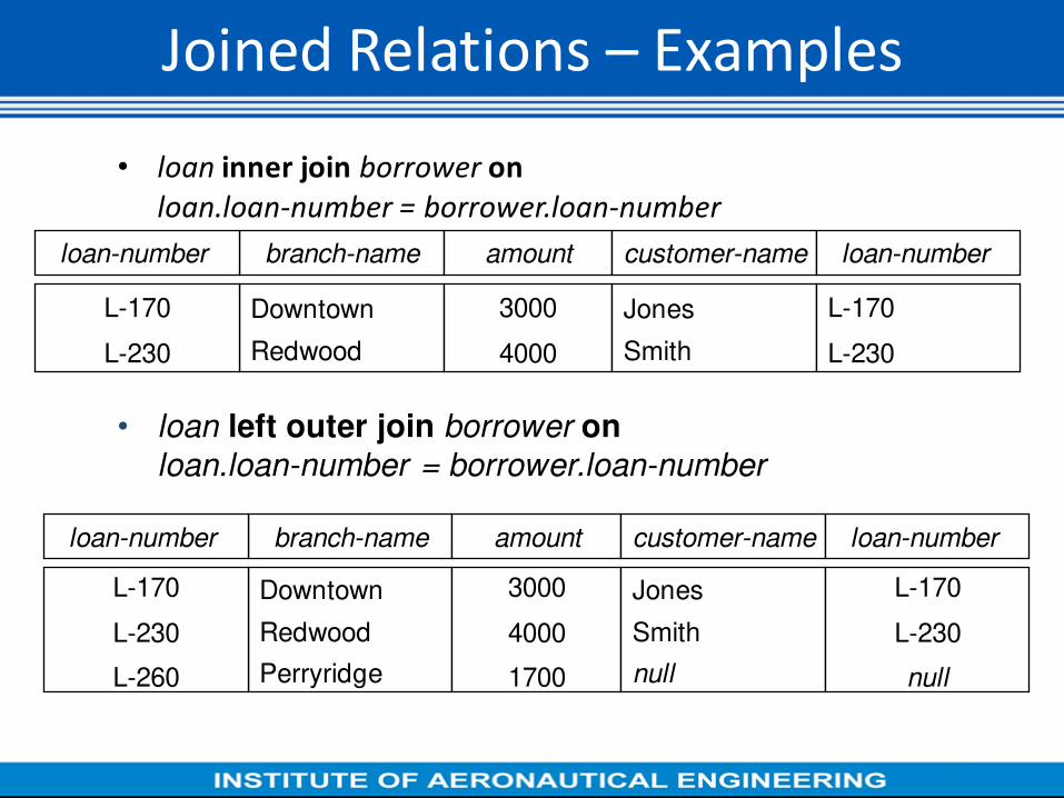
Joined Relations – Examples
• loan inner join borrower on
loan.loan-number = borrower.loan-number
• loan left outer join borrower on
loan.loan-number = borrower.loan-number
branch-name amount
Downtown
Redwood
3000
4000
customer-name loan-number
Jones
Smith
L-170
L-230
loan-number
L-170
L-230
branch-name amount
Downtown
Redwood
Perryridge
3000
4000
1700
customer-name loan-number
Jones
Smith
null
L-170
L-230
null
loan-number
L-170
L-230
L-260

branch-name amount
Downtown
Redwood
3000
4000
customer-name
Jones
Smith
loan-number
L-170
L-230
branch-name amount
Downtown
Redwood
null
3000
4000
null
customer-name
Jones
Smith
Hayes
loan-number
L-170
L-230
L-155
loan natural inner join borrower
loan natural right outer join borrower
Joined Relations – Examples

Joined Relations – Examples
loan full outer join borrower using (loan-number)
branch-name amount
Downtown
Redwood
Perryridge
null
3000
4000
1700
null
customer-name
Jones
Smith
null
Hayes
loan-number
L-170
L-230
L-260
L-155
Find all customers who have either an account or a loan (but not both) at the bank.
select customer-name
from (depositor natural full outer join borrower) where account-number is null or loan-number is null

Views
• Provide a mechanism to hide certain data from the view of certain
users. To create a view we use the command:
• create view v as <query expression>
where:
<query expression> is any legal expression
The view name is represented by v

Update of a View
• Create a view of all loan data in loan relation, hiding the amount
attribute
create view branch-loan as
select branch-name, loan-number from loan
• Add a new tuple to branch-loan
insert into branch-loan
values (‘Perryridge’, ‘L-307’) This insertion must be represented by the insertion of the tuple
(‘L-307’, ‘Perryridge’, null)
into the loan relation
• Updates on more complex views are difficult or impossible to
translate, and hence are disallowed.
• Most SQL implementations allow updates only on simple views
(without aggregates) defined on a single relation

Integrity Constraints - Relational
Database

Integrity Constraints
• Integrity constraints guard against accidental damage to the
database, by ensuring that authorized changes to the
database do not result in a loss of data consistency.
• Various Integrity Constraints In RDB :
– Domain Integrity Constraints
– Referential Integrity Constraints
– Assertions
– Triggers
– Functional Dependencies

Domain Constraints
• Integrity constraints guard against accidental damage to the
database, by ensuring that authorized changes to the database do
not result in a loss of data consistency.
• Domain constraints are the most elementary form of integrity
constraint.
• They test values inserted in the database, and test queries to
ensure that the comparisons make sense.
• New domains can be created from existing data types
– E.g. create domain Dollars numeric(12, 2)
create domain Pounds numeric(12,2)
• We cannot assign or compare a value of type Dollars to a value of
type Pounds.
– However, we can convert type as below
(cast r.A as Pounds)
(Should also multiply by the dollar-to-pound conversion-rate

Referential Integrity • Ensures that a value that appears in one relation for a given set of
attributes also appears for a certain set of attributes in another relation.
– Example: If “Perryridge” is a branch name appearing in one of the tuples in the account relation, then there exists a tuple in the branch relation for branch “Perryridge”.
• Formal Definition
– Let r1(R1) and r2(R2) be relations with primary keys K1 and K2 respectively.
– The subset of R2 is a foreign key referencing K1 in relation r1, if for every t2 in r2 there must be a tuple t1 in r1 such that t1[K1] = t2[].
– Referential integrity constraint also called subset dependency since its can be written as (r2) K1 (r1)

Assertions
• An assertion is a predicate expressing a condition that we wish the
database always to satisfy.
• An assertion in SQL takes the form
create assertion <assertion-name> check <predicate>
• When an assertion is made, the system tests it for validity, and tests
it again on every update that may violate the assertion
– This testing may introduce a significant amount of overhead;
hence assertions should be used with great care.
• Asserting
for all X, P(X)
is achieved in a round-about fashion using
not exists X such that not P(X)

Assertion Example
The sum of all loan amounts for each branch must be less than the
sum of all account balances at the branch.
create assertion sum-constraint check
(not exists (select * from branch
where (select sum(amount) from loan
where loan.branch-name =
branch.branch-name)
>= (select sum(amount) from account
where loan.branch-name =
branch.branch-name)))

Triggers
• A trigger is a statement that is executed automatically by the
system as a side effect of a modification to the database.
• To design a trigger mechanism, we must:
– Specify the conditions under which the trigger is to be executed.
– Specify the actions to be taken when the trigger executes.
• Triggers introduced to SQL standard in SQL:1999, but supported
even earlier using non-standard syntax by most databases.

Trigger Example
• Suppose that instead of allowing negative account balances, the
bank deals with overdrafts by
– setting the account balance to zero
– creating a loan in the amount of the overdraft
– giving this loan a loan number identical to the account number
of the overdrawn account
• The condition for executing the trigger is an update to the account
relation that results in a negative balance value.

Functional Dependencies
Constraints on the set of legal relations.
Require that the value for a certain set of attributes determines
uniquely the value for another set of attributes.
A functional dependency is a generalization of the notion of a
key.

Functional Dependencies (Contd.)
• Let R be a relation schema
R and R
• The functional dependency
holds on R if and only if for any legal relations r(R), whenever any two
tuples t1 and t2 of r agree on the attributes , they also agree on the
attributes . That is,
t1[] = t2 [] t1[ ] = t2 [ ]
• Example: Consider r(A,B) with the following instance of r.
1 4
1 5
3 7
• On this instance, A B does NOT hold, but B A does hold.

Functional Dependencies (Cont.)
• K is a superkey for relation schema R if and only if K R
• K is a candidate key for R if and only if
K R, and
for no K, R
• Functional dependencies allow us to express constraints that cannot be expressed using superkeys.
Consider the schema:
Loan-info-schema = (customer-name, loan-number, branch-name, amount)
We expect this set of functional dependencies to hold:
• loan-number amount
• loan-number branch-name
but would not expect the following to hold:
loan-number customer-name

Pitfalls & Design of Relational
Database

Introduction to schema refinement
• Problems caused by redundancy
Redundant storage
Update Anomalies
Insert Anomalies
Delete Anomalies
Example:
Project ( Project-id, Name, Status, Budget, Dept-Id, Dept-name,
Location)
• How To address Above Problems?
• NULL values can not address completelt

Pitfalls in Relational Database Design
• Relational database design requires that we find a “good” collection of relation schemas. A bad design may lead to
Repetition of Information.
Inability to represent certain information.
• Design Goals:
Avoid redundant data
Ensure that relationships among attributes are represented
Facilitate the checking of updates for violation of database
integrity constraints.

Example Consider the relation schema: Lending-schema = (branch-name,
branch-city, assets , customer-name)
• Redundancy:
Data for branch-name, branch-city, assets are repeated for each loan that a
branch makes
Wastes space
Complicates updating, introducing possibility of inconsistency of assets value
• Null values
Cannot store information about a branch if no loans exist
Can use null values, but they are difficult to handle.

Design Guidelines - RDB
• What is relational database design?
– The grouping of attributes to form "good" relation schemas
• Two levels of relation schemas
– The logical "user view" level
– The storage "base relation" level
• Design is concerned mainly with base relations
• What are the criteria for "good" base relations?

Semantics of the Attributes
• GUIDELINE 1: Informally, each tuple in a relation should represent
one entity or relationship instance. (Applies to individual relations
and their attributes).
– Attributes of different entities (EMPLOYEEs, DEPARTMENTs,
PROJECTs) should not be mixed in the same relation
– Only foreign keys should be used to refer to other entities
– Entity and relationship attributes should be kept apart as much
as possible.
• Bottom Line: Design a schema that can be explained easily relation
by relation. The semantics of attributes should be easy to interpret.

Redundancy - Update Anomalies
• Information is stored redundantly
– Wastes storage
– Causes problems with update anomalies
• Insertion anomalies
• Deletion anomalies
• Modification anomalies

UPDATE ANOMALY- EXAMPLE
• Consider the relation:
– EMP_PROJ(Emp#, Proj#, Ename, Pname, No_hours)
• Update Anomaly:
– Changing the name of project number P1 from “Billing” to “Customer-Accounting” may cause this update to be made for all 100 employees working on project P1.

INSERT ANOMALY - EXAMPLE
• Consider the relation:
– EMP_PROJ(Emp#, Proj#, Ename, Pname, No_hours)
• Insert Anomaly:
– Cannot insert a project unless an employee is assigned to it.
• Conversely
– Cannot insert an employee unless an he/she is assigned to a
project.

DELETE ANOMALY- EXAMPLE
• Consider the relation:
– EMP_PROJ(Emp#, Proj#, Ename, Pname, No_hours)
• Delete Anomaly:
– When a project is deleted, it will result in deleting all the
employees who work on that project.
– Alternately, if an employee is the sole employee on a project,
deleting that employee would result in deleting the
corresponding project.

Redundancy - Update Anomalies
• GUIDELINE 2:
– Design a schema that does not suffer from the insertion,
deletion and update anomalies.
– If there are any anomalies present, then note them so that
applications can be made to take them into account.

Null Values in Tuples
• GUIDELINE 3:
– Relations should be designed such that their tuples will have as
few NULL values as possible
– Attributes that are NULL frequently could be placed in separate
relations (with the primary key)
• Reasons for nulls:
– Attribute not applicable or invalid
– Attribute value unknown (may exist)
– Value known to exist, but unavailable

Spurious Tuples – avoid at any cost
• Bad designs for a relational database may result in erroneous results for certain JOIN operations
• The "lossless join" property is used to guarantee meaningful results for join operations
• GUIDELINE 4: – The relations should be designed to satisfy the lossless join
condition.
– No spurious tuples should be generated by doing a natural-join of any relations.

Spurious Tuples
• There are two important properties of decompositions:
a) Non-additive or losslessness of the corresponding join
b) Preservation of the functional dependencies.
• Note that:
– Property (a) is extremely important and cannot be sacrificed.
– Property (b) is less stringent and may be sacrificed. (See
Chapter 15).

Overall Database Design Process
• We have assumed schema R is given
R could have been generated when converting E-R diagram to a set of tables.
R could have been a single relation containing all attributes that are of interest (called universal relation).
Normalization breaks R into smaller relations.
R could have been the result of some ad hoc design of relations, which we then test/convert to normal form.

Functional Dependencies -
Reasoning

Functional Dependencies
– Constraints on the set of legal relations.
– Require that the value for a certain set of attributes determines
uniquely the value for another set of attributes.
– A functional dependency is a generalization of the notion of a
key.

Functional Dependencies (Contd.) • Let R be a relation schema
R and R
• The functional dependency
holds on R if and only if for any legal relations r(R), whenever any two
tuples t1 and t2 of r agree on the attributes , they also agree on the
attributes . That is,
t1[] = t2 [] t1[ ] = t2 [ ]
• Example: Consider r(A,B) with the following instance of r.
1 4
1 5
3 7
• On this instance, A B does NOT hold, but B A does hold.

Functional Dependencies (Cont.)
• K is a superkey for relation schema R if and only if K R
• K is a candidate key for R if and only if
K R, and
for no K, R
• Functional dependencies allow us to express constraints that cannot be expressed using superkeys.
Consider the schema:
Loan-info-schema = (customer-name, loan-number, branch-name, amount)
We expect this set of functional dependencies to hold:
• loan-number amount
• loan-number branch-name
but would not expect the following to hold:
loan-number customer-name

Use of Functional Dependencies
• We use functional dependencies to:
test relations to see if they are legal under a given set of functional dependencies
• If a relation r is legal under a set F of functional dependencies, we say that r satisfies F.
specify constraints on the set of legal relations
• We say that F holds on R if all legal relations on R satisfy the set of functional dependencies F.
• Note: A specific instance of a relation schema may satisfy a functional dependency even if the functional dependency does not hold on all legal instances.
For example, a specific instance of Loan-schema may, by chance, satisfy
loan-number customer-name.

Closure of a Set of Functional Dependencies
• Given a set F set of functional dependencies, there are certain
other functional dependencies that are logically implied by F.
E.g. If A B and B C, then we can infer that A C
• The set of all functional dependencies logically implied by F is the
closure of F.
• We denote the closure of F by F+.
• We can find all of F+ by applying Armstrong’s Axioms:
if , then
if , then
if , and , then
• These rules are
(reflexivity)
(augmentation)
(transitivity)
sound (generate only functional dependencies that actually hold) and
complete (generate all functional dependencies that hold).

Example R = (A, B, C, G, H, I)
F = {
A B
A C
CG H
CG I
B H }
some members of F+
A H
by transitivity from A B and B H
AG I
by augmenting A C with G, to get AG CG
and then transitivity with CG I
CG HI
from CG H and CG I : “union rule” can be inferred from
– definition of functional dependencies, or
– Augmentation of CG I to infer CG CGI, augmentation of
CG H to infer CGI HI, and then transitivity

Decomposition – Desirable
Properties

Decomposition - Problems
• To Avoid Redundancy the given relations must be Decomposed into
Sub Relations.
• Problems related to Decomposition
Lossy /Superfluous information
Dependency Preservation
Solution: Lossless Join Decomposition

Decomposition
• Decompose the relation schema Lending-schema into:
Branch-schema = (branch-name, branch-city , assets)
Loan-info-schema = (customer-name, loan-number, branch-name,
amount)
• All attributes of an original schema (R) must appear in the
decomposition (R1, R2):
R = R1 R2
• Lossless-join decomposition.
For all possible relations r on schema R
r = R1 (r) R2 (r)

Example of Non Lossless-Join Decomposition
• Decomposition of R = (A, B) R1 = (A) R2 = (B)
A B
1
2
1
A
B
1
2
A(r) B(r)
r
A (r) B (r) A B
1
2
1
2

Dependency Preservation
• After Decomposing Relation into Sub relations each FD that hold on
original relation must hold on any of sub relation

Testing for Dependency Preservation
• To check if a dependency is preserved in a decomposition of
R into R1, R2, …, Rn we apply the following simplified test (with
attribute closure done w.r.t. F)
result = while (changes to result) do
for each Ri in the decomposition
t = (result Ri)+ Ri
result = result t
If result contains all attributes in , then the functional
dependency is preserved.
• We apply the test on all dependencies in F to check if a
decomposition is dependency preserving
• This procedure takes polynomial time, instead of the exponential
time required to compute F+ and (F1 F2 … Fn)+

Goals of Normalization
Decide whether a particular relation R is in “good” form.
In the case that a relation R is not in “good” form, decompose it
into a set of relations {R1, R2, ..., Rn} such that
• each relation is in good form
• the decomposition is a lossless-join decomposition
Our theory is based on:
• functional dependencies
• multivalued dependencies

Normalization Using Functional Dependencies
• When we decompose a relation schema R with a set of functional
dependencies F into R1, R2,.., Rn we want
Lossless-join decomposition: Otherwise decomposition would result in information loss.
No redundancy: The relations Ri preferably should be in either Boyce- Codd Normal Form or Third Normal Form.
Dependency preservation: Let Fi be the set of dependencies F+ that include only attributes in Ri.
Preferably the decomposition should be dependency preserving,
that is (F1 F2 … Fn)
+ = F+
Otherwise, checking updates for violation of functional dependencies
may require computing joins, which is expensive.

Example
• R = (A, B, C)
F = {A B, B C)
Can be decomposed in two different ways
• R1 = (A, B), R2 = (B, C)
Lossless-join decomposition:
R1 R2 = {B} and B BC
Dependency preserving
• R1 = (A, B), R2 = (A, C)
Lossless-join decomposition:
R1 R2 = {A} and A AB
Not dependency preserving
(cannot check B C without computing R1 R2)

Testing for Dependency Preservation
• To check if a dependency is preserved in a decomposition of
R into R1, R2, …, Rn we apply the following simplified test (with
attribute closure done w.r.t. F)
result = while (changes to result) do
for each Ri in the decomposition
t = (result Ri)+ Ri
result = result t
If result contains all attributes in , then the functional
dependency is preserved.
• We apply the test on all dependencies in F to check if a
decomposition is dependency preserving
• This procedure takes polynomial time, instead of the exponential
time required to compute F+ and (F1 F2 … Fn)+

Normalization of Relations
• Normalization: – The process of decomposing unsatisfactory "bad" relations by
breaking up their attributes into smaller relations
• Normal form: – Condition using keys and FDs of a relation to certify whether a
relation schema is in a particular normal form

Normalization of Relations (2)
• 2NF, 3NF, BCNF – based on keys and FDs of a relation schema
• 4NF
– based on keys, multi-valued dependencies : MVDs;
• 5NF
– based on keys, join dependencies : JDs
• Additional properties may be needed to ensure a good relational
design (lossless join, dependency preservation; see Chapter 15)

Practical Use of Normal Forms
• Normalization is carried out in practice so that the resulting designs are of high quality and meet the desirable properties
• The practical utility of these normal forms becomes questionable when the constraints on which they are based are hard to understand or to detect
• The database designers need not normalize to the highest possible normal form
– (usually up to 3NF and BCNF. 4NF rarely used in practice.)
• Denormalization:
– The process of storing the join of higher normal form relations
as a base relation—which is in a lower normal form

Keys and Attributes
• A superkey of a relation schema R = {A1, A2, ...., An} is a set of
attributes S subset-of R with the property that no two tuples t1 and
t2 in any legal relation state r of R will have t1[S] = t2[S]
• A key K is a superkey with the additional property that
removal of any attribute from K will cause K not to be a superkey
any more.

Keys and Attributes
• If a relation schema has more than one key, each is called a
candidate key.
– One of the candidate keys is arbitrarily designated to be the
primary key, and the others are called secondary keys.
• A Prime attribute must be a member of some candidate key
• A Nonprime attribute is not a prime attribute—that is, it is not
a member of any candidate key.

First Normal Form
• Disallows – composite attributes
– multivalued attributes
– nested relations; attributes whose values for an individual tuple
are non-atomic
• Considered to be part of the definition of a relation
• Most RDBMSs allow only those relations to be defined that are in
First Normal Form

Normalization into 1NF

Second Normal Form (1)
• Uses the concepts of FDs, primary key
• Definitions
– Prime attribute: An attribute that is member of the primary key K
– Full functional dependency: a FD Y -> Z where removal of
any attribute from Y means the FD does not hold any more
• Examples:
– {SSN, PNUMBER} -> HOURS is a full FD since neither SSN -> HOURS nor PNUMBER -> HOURS hold
– {SSN, PNUMBER} -> ENAME is not a full FD (it is called a partial dependency ) since SSN -> ENAME also holds

Second Normal Form (2)
• A relation schema R is in second normal form (2NF) if every non-
prime attribute A in R is fully functionally dependent on the primary
key
• R can be decomposed into 2NF relations via the process of 2NF
normalization or “second normalization”

Normalizing into 2NF and 3NF

Third Normal Form & BCNF

Third Normal Form (1)
• Definition:
– Transitive functional dependency: a FD X -> Z that can be derived from two FDs X -> Y and Y -> Z
• Examples:
– SSN -> DMGRSSN is a transitive FD • Since SSN -> DNUMBER and DNUMBER -> DMGRSSN hold
– SSN -> ENAME is non-transitive
• Since there is no set of attributes X where SSN -> X and X -> ENAME

Third Normal Form (2)
• A relation schema R is in third normal form (3NF) if it is in 2NF and no non-prime attribute A in R is transitively dependent on the primary key
• R can be decomposed into 3NF relations via the process of 3NF normalization
• NOTE: – In X -> Y and Y -> Z, with X as the primary key, we consider this a
problem only if Y is not a candidate key.
– When Y is a candidate key, there is no problem with the transitive dependency .
– E.g., Consider EMP (SSN, Emp#, Salary ).
• Here, SSN -> Emp# -> Salary and Emp# is a candidate key

Normal Forms Defined Informally
• 1st normal form
– All attributes depend on the key
• 2nd normal form
– All attributes depend on the whole key
• 3rd normal form
– All attributes depend on nothing but the key

General Definition of 2NF
• A relation schema R is in second normal form (2NF) if every non-
prime attribute A in R is fully functionally dependent on every key
of R
• FD
County_name → Tax_rate violates 2NF.
So second normalization converts LOTS into
LOTS1 (Property_id#, County_name, Lot#, Area, Price)
LOTS2 ( County_name, Tax_rate)

Third Normal Form
• DEFINITION of 3NF: A relation schema R is in third normal form (3NF) if every non-
prime attribute in R meets both of these conditions:
– It is fully functionally dependent on every key of R
– It is non-transitively dependent on every key of R
Note that stated this way, a relation in 3NF also meets the
requirements for 2NF.

BCNF (Boyce-Codd Normal Form)
• A relation schema R is in Boyce-Codd Normal Form (BCNF) if
whenever an FD X → A holds in R, then X is a superkey of R
• Each normal form is strictly stronger than the previous one
– Every 2NF relation is in 1NF
– Every 3NF relation is in 2NF
– Every BCNF relation is in 3NF
• There exist relations that are in 3NF but not in BCNF
• Hence BCNF is considered a stronger form of 3NF
• The goal is to have each relation in BCNF (or 3NF)

BCNF - Example

BCNF by Decomposition (1)
• Two FDs exist in the relation TEACH:
– fd1: { student, course} -> instructor
– fd2: instructor -> course
• {student, course} is a candidate key for this relation and that the dependencies shown follow the pattern in Figure 14.13 (b).
– So this relation is in 3NF but not in BCNF
• A relation NOT in BCNF should be decomposed so as to meet this property, while possibly forgoing the preservation of all functional dependencies in the decomposed relations.

BCNF by Decomposition (2)
• Three possible decompositions for relation TEACH – D1: {student, instructor} and {student, course} – D2: {course, instructor } and {course, student} – D3: {instructor, course } and {instructor, student}
• All three decompositions will lose fd1. – We have to settle for sacrificing the functional dependency
preservation. But we cannot sacrifice the non-additivity property after decomposition.
• Out of the above three, only the 3rd decomposition will not generate spurious tuples after join.(and hence has the non-additivity property).
• A test to determine whether a binary decomposition
(decomposition into two relations) is non-additive (lossless) is discussed under Property NJB on the next slide. We then show how the third decomposition above meets the property.

MULTIVALUED DEPENDENCIES
JOIN DEPENDENCIES
4NF & 5NF

Multivalued Dependencies
There are database schemas in BCNF that do not seem to be
sufficiently normalized
Consider a database
• classes(course, teacher, book)
• such that (c,t,b) classes means that t is qualified to teach c,
• and b is a required textbook for c
The database is supposed to list for each course the set of teachers
any one of which can be the course’s instructor, and the set of
books, all of which are required for the course (no matter who
teaches it).

Multivalued Dependencies (Contd.)
There are no non-trivial functional dependencies and
therefore the relation is in BCNF
Insertion anomalies – i.e., if Sara is a new teacher that can teach
classes Insertion anomalies – i.e., if Sara is a new teacher that can teach
the following two tuples need to be inserted
(Physics101, Sara, Mechanics)
(database, Sara, Optics)

Multivalued Dependencies (MVDs)
Let R be a relation schema and let R and R.
The multivalued dependency
holds on R if in any legal relation r(R), for all pairs for tuples t1
and t2 in r such that t1[] = t2 [], there exist tuples t3 and t4 in r
such that:
t1[] = t2 [] = t3 [] t4 []
t3[] = t1 []
t3[R– ] = t2[R – ]
t4 [] = t2[]
t4[R– ] = t1[R– ]

EXAMPLE
Let R be a relation schema with a set of attributes that are
partitioned into 3 nonempty subsets.
• Y, Z, W
We say that Y Z (Y multidetermines Z)
• if and only if for all possible relations r(R)
• < y1, z1, w1 > r and < y2, z2, w2 > r
• then
• < y1, z1, w2 > r and < y2, z2, w1 > r
Note that since the behavior of Z and W are identical it follows that Y Z if Y W

EXAMPLE Contd.
In our example:
• course teacher
• course book
The above formal definition is supposed to formalize the notion that given a particular value of Y (course) it has associated with it a set of values of Z (teacher) and a set of values of W (book), and these two sets are in some sense independent of each other.
Note:
• If Y Z then Y Z
• Indeed we have (in above notation) Z1 = Z2
The claim follows.

Use of Multivalued Dependencies
We use multivalued dependencies in two ways:
1. To test relations to determine whether they are legal under a
given set of functional and multivalued dependencies
2. To specify constraints on the set of legal relations. We shall thus
concern ourselves only with relations that satisfy a given set of
functional and multivalued dependencies.
If a relation r fails to satisfy a given multivalued dependency, we
can construct a relations r that does satisfy the
multivalued dependency by adding tuples to r

Theory of MVDs From the definition of multivalued dependency, we can derive
the following rule:
• If , then
• That is, every functional dependency is also a
multivalued dependency
The closure D+ of D is the set of all functional and
multivalued dependencies logically implied by D.
• We can compute D+ from D, using the formal definitions of functional dependencies and multivalued dependencies.
• We can manage with such reasoning for very simple multivalued dependencies, which seem to be most common in practice
• For complex dependencies, it is better to reason about
sets of dependencies using a system of inference rules .

Fourth Normal Form
A relation schema R is in 4NF with respect to a set D of
functional and multivalued dependencies if for all multivalued
dependencies in D+ of the form , where R and
R, at least one of the following hold:
• is trivial (i.e., or = R)
• is a superkey for schema R
If a relation is in 4NF it is in BCNF

Join Dependencies and 5NF
Definition:
• A join dependency (JD), denoted by JD(R1, R2, ..., Rn), specified on
relation schema R, specifies a constraint on the states r of R.
– The constraint states that every legal state r of R should have
a non-additive join decomposition into R1, R2, ..., Rn; that is,
for every such r we have
– * (R1(r), R2(r), ..., Rn(r)) = r
Note: an MVD is a special case of a JD where n = 2.
• A join dependency JD(R1, R2, ..., Rn), specified on relation schema
R, is a trivial JD if one of the relation schemas Ri in JD(R1, R2, ...,
Rn) is equal to R.

Join Dependencies & 5NF Contd..
Definition:
• A relation schema R is in fifth normal form (5NF) (or
Project-Join Normal Form (PJNF)) with respect to a set F of
functional, multivalued, and join dependencies if,
– for every nontrivial join dependency JD(R1, R2, ..., Rn) in
F+ (that is, implied by F),
• every Ri is a superkey of R.
• Discovering join dependencies in practical databases with
hundreds of relations is next to impossible. Therefore, 5NF
is rarely used in practice.

ER Model and Normalization
&
Universal Relation Approach

Overall Database Design Process
We have assumed schema R is given
• R could have been generated when converting E-R diagram to a set of tables.
• R could have been a single relation containing all attributes
that are of interest (called universal relation).
• Normalization breaks R into smaller relations.
• R could have been the result of some ad hoc design of relations, which we then test/convert to normal form.

ER Model and Normalization
Dangling tuples – Tuples that “disappear” in
computing a join.
• Let r1 (R1), r2 (R2), …., rn (Rn) be a set of relations
• A tuple r of the relation ri is a dangling tuple if r is not in the
relation join of all sub relations r1,r2,…rn
• The relation r1 r2…. Is a universal relation that involves all
the attributes in the “universe” defined by R1 R2 … Rn
• If dangling tuples are allowed in the database, instead of
decomposing a universal relation, we may prefer to
synthesize a collection of normal form schemas from a given
set of attributes.

Universal Relation Approach
Dangling tuples may occur in practical database applications.
They represent incomplete information
E.g. may want to break up information about loans into:
• (branch-name, loan-umber)
(loan-number, amount)
• (loan-number, customer-name)
Universal relation would require null values, and have dangling
tuples

Universal Relation Approach Contd. A particular decomposition defines a restricted
form of incomplete information that is acceptable in our database.
• Above decomposition requires at least one of customer-name, branch-name or amount in order to enter a loan number without using null values
• Rules out storing of customer-name, amount without an appropriate loan-number (since it is a key, it can't be null either!)
Universal relation requires unique attribute names unique role assumption
• e.g. customer-name, branch-name
Reuse of attribute names is natural in SQL since relation names can be prefixed to disambiguate names

UNIT - IV
Transaction - Concept, properties
and state

Transaction: A transaction is a unit of program execution that accesses and possibly
updates various data items.
• E.g., transaction to transfer $50 from account A to account B:
1. read(A)
2. A := A – 50
3. write(A)
4. read(B)
5. B := B + 50
6. write(B)

Two main issues to deal with:
– Failures of various kinds, such as hardware failures and system
crashes
– Concurrent execution of multiple transactions

Required Properties of a Transaction
• Consider a transaction to transfer $50 from account A to
account B:
1. read(A)
2. A := A – 50
3. write(A)
4. read(B)
5. B := B + 50
6. write(B)

Atomicity requirement – If the transaction fails after step 3 and before step 6, money will
be “lost” leading to an inconsistent database state
• Failure could be due to software or hardware
– The system should ensure that updates of a partially executed transaction are not reflected in the database
Durability requirement :
once the user has been notified that the transaction has completed
(i.e., the transfer of the $50 has taken place), the updates to the database by the transaction must persist even if there are software or hardware failures.

Consistency requirement: In above example:
– The sum of A and B is unchanged by the execution of the transaction
• In general, consistency requirements include
• Explicitly specified integrity constraints such as primary keys and foreign keys
• Implicit integrity constraints
– e.g., sum of balances of all accounts, minus sum of loan amounts must equal value of cash-in-hand
• A transaction, when starting to execute, must see a consistent database.
• During transaction execution the database may be temporarily inconsistent.
• When the transaction completes successfully the database must be consistent

Isolation requirement :
If between steps 3 and 6 (of the fund transfer transaction) , another transaction T2 is allowed to access the partially updated database, it will see an inconsistent database (the sum A + B will be less than it should be).
T1 T2
1. read(A)
2. A := A – 50
3. write(A) read(A), read(B), print(A+B)
4. read(B)
5. B := B + 50
6. write(B
• Isolation can be ensured trivially by running transactions serially
– That is, one after the other.

ACID Properties
A transaction is a unit of program execution that accesses and
possibly updates various data items. To preserve the integrity of
data the database system must ensure:
• Atomicity. Either all operations of the transaction are properly
reflected in the database or none are.
• Consistency. Execution of a transaction in isolation preserves the
consistency of the database.

ACID Properties(cont.)
• Isolation. Although multiple transactions may execute
concurrently, each transaction must be unaware of other
concurrently executing transactions. Intermediate transaction
results must be hidden from other concurrently executed
transactions.
– That is, for every pair of transactions Ti and Tj, it appears to Ti
that either Tj, finished execution before Ti started, or Tj started
execution after Ti finished.
• Durability. After a transaction completes successfully, the changes
it has made to the database persist, even if there are system
failures.

Transaction State
• Active – the initial state; the transaction stays in this state while it is
executing
• Partially committed – after the final statement has been executed.
• Failed -- after the discovery that normal execution can no longer
proceed.

Transaction State(cont.)
• Aborted – after the transaction has been rolled back and the
database restored to its state prior to the start of the transaction.
Two options after it has been aborted:
– Restart the transaction
• can be done only if no internal logical error
– Kill the transaction
• Committed – after successful completion.

Transaction State (Cont.)

Transaction Management
Implementation of atomicity,
consistency, isolation and
durability

Implementation of Atomicity an Durability
• Atomicity
– Transactions are atomic – they don’t have parts (conceptually) – can’t be executed partially; it should not be detectable that they
interleave with another transaction
• Durability – Once a transaction has completed, its changes are made
permanent
– Even if the system crashes, the effects of a transaction must remain in place

Atomicity an Durability(cont.)
• To implement the Atomicity an Durability we use a technique called
shadow copy scheme.
• It uses a database pointer to refer the copy of file in the database.

Implementation of Isolation
• Isolation
– The effects of a transaction are not visible to other transactions until it has completed
– From outside the transaction has either happened or not
• There are various concurrency control schemes that ensures that a
transaction has to acquire locks
• Concurrency control scheme provides few locking protocols to
ensure the concurrent execution.

Consistency
Consistency
Transactions take the database from one consistent state
into another
In the middle of a transaction the database might not be
consistent.

Example of transaction
• Transfer £50 from account A to account B
Read(A)
A = A - 50
Write(A)
Read(B)
B = B+50
Write(B)
Atomicity - shouldn’t take money from A without giving it to B
Consistency - money isn’t lost or gained
Isolation - other queries shouldn’t see A or B change until completion
Durability - the money does not go back to A

• The transaction manager enforces the ACID properties
– It schedules the operations of transactions
– COMMIT and ROLLBACK are used to ensure atomicity

Transaction Management
Concurrent execution and
Recoverability of Transactions

Concurrent Executions
• Multiple transactions are allowed to run concurrently in the system.
Advantages are:
– Increased processor and disk utilization, leading to
better transaction throughput
• E.g. one transaction can be using the CPU while another is
reading from or writing to the disk
– Reduced average response time for transactions: short
transactions need not wait behind long ones.

Concurrent Executions(cont.)
• Concurrency control schemes – mechanisms to achieve
isolation
– That is, to control the interaction among the concurrent
transactions in order to prevent them from destroying the
consistency of the database

Example : let T1 & T2 are two transactions that transfers funds from one account to another.
Step-1:- Transaction T1 transfers 500 from account A to account B is defined as
T1: Read(A)
A:=A-500;
Write(A);
Read(B);
B:=B+500;
Write(B);
T2 : Read(A)
temp:=A*0.1;
A:=A-temp;
Write(A);
Read(B);
B:=B+temp;
Write(B);

A serial schedule in which T1 is followed by T2
T1
Read(A);
A:=A-500;
Write(A);
Read(B);
B:=B+500;
Write(B);
T2
Read(A);
temp:=A*0.1;
A:=A-temp;
Write(A);
Read(B);
B:=B+temp;
Write(B);
* Vice versa for T2 is followed by T1

Concurrent schedule:
T1
Read(A);
A:=A-500;
Write(A);
Read(B);
B:=B+500;
Write(B);
T2
Read(A);
temp:=A*0.1; A:=A-temp; Write(A);
Read(B); B:=B+temp;
Write(B);
Concurrent execution is carried out by concurrency-control component
of the database.

Recoverability
• A schedule is said to be recoverable if a failed transaction is
undone.
If a transaction Ti fails we need to undo the effect of this transaction
to ensure the atomicity property.
In a concurrent execution it is necessary to ensure that transaction
Ti that is dependent on Ti is also aborted.

Recoverable Schedules
• Recoverable schedule — if a transaction Tj reads a data item previously written by a transaction Ti , then the commit operation of Ti must appear before the commit operation of Tj.
• The following schedule is not recoverable if T9 commits immediately after the read(A) operation.
If T8 should abort, T9 would have read (and possibly shown to the
user) an inconsistent database state. Hence, database must ensure
that schedules are recoverable.

Cascading Rollbacks
• Cascading rollback – a single transaction failure leads to a series
of transaction rollbacks. Consider the following schedule where
none of the transactions has yet committed (so the schedule is
recoverable)
If T10 fails, T11 and T12 must also be rolled back.
Can lead to the undoing of a significant amount of work

Cascadeless Schedules
• Cascadeless schedules — for each pair of transactions Ti and Tj
such that Tj reads a data item previously written by Ti, the commit
operation of Ti appears before the read operation of Tj.
• Every cascadeless schedule is also recoverable
• It is desirable to restrict the schedules to those that are cascadeless
• Example of a schedule that is NOT cascadeless

Concurrency Control
• A database must provide a mechanism that will ensure that all possible schedules are both:
– Conflict serializable.
– Recoverable and preferably cascadeless
• Concurrency-control schemes tradeoff between the amount of concurrency they allow and the amount of overhead that they incur
• Testing a schedule for serializability after it has executed is a little too late!
– Tests for serializability help us understand why a concurrency control protocol is correct
• Goal – to develop concurrency control protocols that will assure serializability.

Transaction Management
Serializability - View and Conflict

Serializability
• Basic Assumption – Each transaction preserves database
consistency.
• Thus, serial execution of a set of transactions preserves database
consistency.
• A (possibly concurrent) schedule is serializable if it is equivalent to a
serial schedule. Different forms of schedule equivalence give rise to
the notions of:
1. conflict serializability
2. view serializability

Simplified view of transactions
• We ignore operations other than read and write instructions
• We assume that transactions may perform arbitrary
computations on data in local buffers in between reads and
writes.
• Our simplified schedules consist of only read and write
instructions.

Conflicting Instructions
Let li and lj be two Instructions of transactions Ti and Tj
respectively. Instructions li and lj conflict if and only if there exists
some item Q accessed by both li and lj, and at least one of these
instructions wrote Q.
1. li = read(Q), lj = read(Q). li and lj don’t conflict. 2. li = read(Q), lj = write(Q). They conflict.
3. li = write(Q), lj = read(Q). They conflict
4. li = write(Q), lj = write(Q). They conflict

Conflicting Instructions(cont.)
Intuitively, a conflict between li and lj forces a (logical) temporal order
between them.
If li and lj are consecutive in a schedule and they do not conflict,
their results would remain the same even if they had been
interchanged in the schedule.

Conflict Serializability
If a schedule S can be transformed into a schedule S´ by a series
of swaps of non-conflicting instructions, we say that S and S´ are
conflict equivalent.
We say that a schedule S is conflict serializable if it is conflict
equivalent to a serial schedule

Conflict Serializability (Cont.)
Schedule 3 can be transformed into Schedule 6 -- a serial schedule
where T2 follows T1, by a series of swaps of non-conflicting
instructions. Therefore, Schedule 3 is conflict serializable.
Schedule 3 Schedule 6

Conflict Serializability (Cont.)
• Example of a schedule that is not conflict serializable:
We are unable to swap instructions in the above schedule to
obtain either the serial schedule < T3, T4 >, or the serial schedule
< T4, T3 >.

View Serializability
• Let S and S’ be two schedules with the same set of transactions . And S’ are View equivalent if the following three conditions are met:
1. Initial Read
2. Write-read
3. Final write
• View equivalence is purely based on reads and writes alone.

View Serializability(cont.)
• A schedule S is view serializable it is equivalent to a serial schedule.
• Every conflict serializable schedule is also a view serializable .
• Every view serializable schedule is not conflict serializable has
blind writes.
Above example is a view serializable but not conflict serializable.

Transaction Management
Testing Serializability,
Concurrency Control vs.
Serializability Tests

Testing for Conflict Serializability
• In order to determine a conflict serializable we need to
construct a directed graph called precedence graph .
• It is represented as G=(V,E)
• V-consists of transactions
• E-consists of set of edges Ti->Tj for which one of the three
conditions.
1. Ti executes Write(Q) before Tj executes Read(Q).
2. Ti executes Read(Q) before Tj executes Write(Q)
3. Ti executes Write(Q) before Tj executes Write(Q)

Testing for Conflict Serializability(cont.)
• A schedule is conflict serializable if and only if its precedence
graph is acyclic.
• Cycle-detection algorithms exist which take order n2 time,
where n is the number of vertices in the graph.
– (Better algorithms take order n + e where e is the number
of edges.)
• If precedence graph is acyclic, the serializability order can be
obtained by a topological sorting of the graph.
– That is, a linear order consistent with the partial order of
the graph.

Precedence Graph
Consider some schedule of a set of transactions T1, T2, ..., Tn
Precedence graph — a direct graph where the vertices are the
transactions (names).
We draw an arc from Ti to Tj if the two transaction conflict, and Ti
accessed the data item on which the conflict arose earlier.
We may label the arc by the item that was accessed.
Example

Conflict Serializability
For example, a serializability order for
the schedule (a) would be one of
either (b) or (c)

Concurrency Control vs. Serializability Tests
• Concurrency-control protocols allow concurrent schedules, but
ensure that the schedules are conflict/view serializable, and are
recoverable and cascadeless .
• Different concurrency control protocols provide different
tradeoffs between the amount of concurrency they allow and
the amount of overhead that they incur.
• Tests for serializability help us understand why a concurrency
control protocol is correct.

Concurrency Control
• A database must provide a mechanism that will ensure that all possible
schedules are both:
– Conflict serializable.
– Recoverable and preferably cascadeless
• A policy in which only one transaction can execute at a time generates serial
schedules, but provides a poor degree of concurrency
• Concurrency-control schemes tradeoff between the amount of concurrency
they allow and the amount of overhead that they incur.
• Testing a schedule for serializability after it has executed is a little too late!
– Tests for serializability help us understand why a concurrency control
protocol is correct
• Goal – to develop concurrency control protocols that will assure
serializability.

Weak Levels of Consistency
• Some applications are willing to live with weak levels of consistency,
allowing schedules that are not serializable
– E.g., a read-only transaction that wants to get an approximate
total balance of all accounts
– E.g., database statistics computed for query optimization can be
approximate (why?)
– Such transactions need not be serializable with respect to other
transactions
• Tradeoff accuracy for performance

Levels of Consistency in SQL-92
• Serializable — default
• Repeatable read — only committed records to be read,
repeated reads of same record must return same value. However, a
transaction may not be serializable – it may find some records
inserted by a transaction but not find others.
• Read committed — only committed records can be read, but
successive reads of record may return different (but committed)
values.
• Read uncommitted — even uncommitted records may be read.

Levels of Consistency in SQL-92(cont.)
Lower degrees of consistency useful for gathering approximate
information about the database
Warning: some database systems do not ensure serializable
schedules by default
E.g., Oracle and PostgreSQL by default support a level of
consistency called snapshot isolation (not part of the SQL
standard)

Transaction Definition in SQL
• Data manipulation language must include a construct for specifying
the set of actions that comprise a transaction.
• In SQL, a transaction begins implicitly.
• A transaction in SQL ends by:
– Commit work commits current transaction and begins a new
one.
– Rollback work causes current transaction to abort.
• In almost all database systems, by default, every SQL statement also
commits implicitly if it executes successfully
– Implicit commit can be turned off by a database directive
• E.g. in JDBC, connection.setAutoCommit(false);

Transaction Management
Introduction to Locks - types,
granting lock

Introduction:
Locking is necessary in a concurrent environment to assure that
one process should not retrieve or update a record which another
process is updating. Failure to this would result in inconsistent and
corrupted data.

There are various modes to lock data items. They are:
• Shared(S): If a transaction Ti has shared mode lock on data item Q
then Ti can read but not write Q. lock-S(Q) instruction is used in
shared mode.
• Exclusive(X): If a transaction has obtained an exclusive mode lock
on data item Q, then Ti can perform both read and write. lock-X(Q)
instruction is used to lock in exclusive mode.
Types of Locks
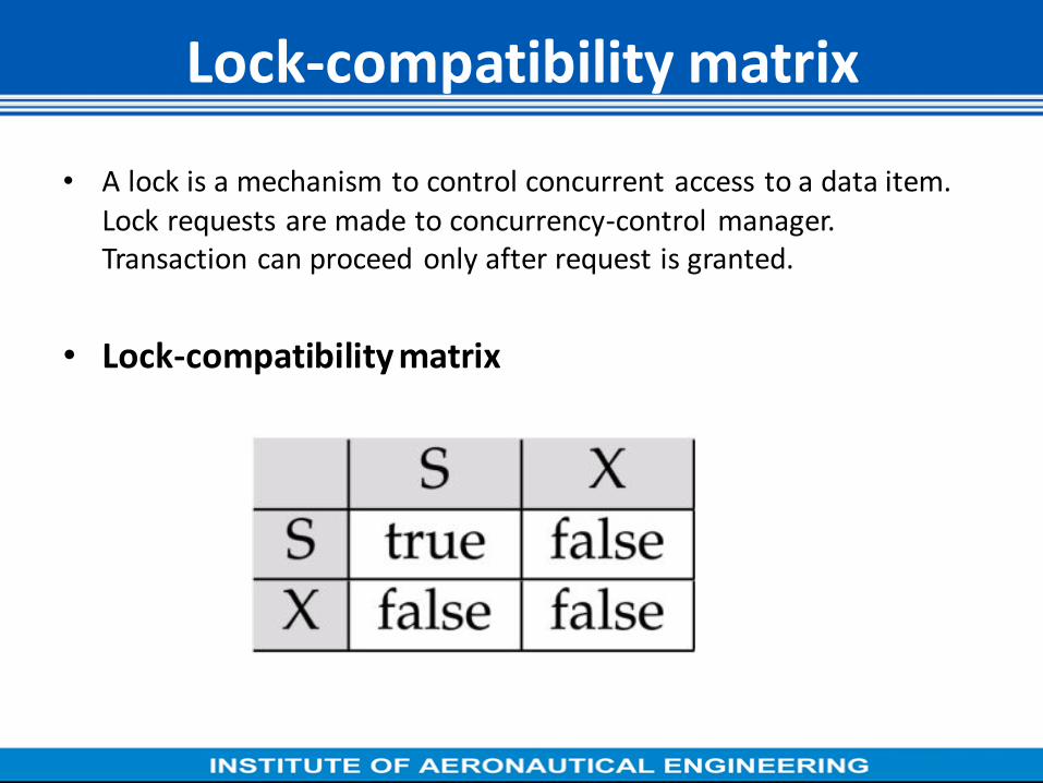
• A lock is a mechanism to control concurrent access to a data item.
Lock requests are made to concurrency-control manager.
Transaction can proceed only after request is granted.
• Lock-compatibility matrix
Lock-compatibility matrix

Example of a transaction performing locking:
Locking as above is not sufficient to guarantee serializability — if A and
B get updated in-between the read of A and B, the displayed sum would
be wrong.

Granting of Locks
Concurrency control manager will grants the lock requests to the
transactions.
•First it checks for no access on that particular data item it allocates
lock on that data item.
•Else it keeps the requesting transaction in waiting state.

Transaction Management
Lock based protocols

Lock-based Protocols
Lock-based Protocols:
lock-based protocols use a mechanism by which any transaction
cannot read or write data until it acquires an appropriate lock on it.

Problems with Locking
• Transaction schedule may not be serializable
₋ Can be solved with Two-Phase Locking
• May cause deadlocks
₋ A deadlock is caused when two transactions wait for each
other to unlock data.

Two-Phase Locking (2PL)
Two-Phase Locking (2PL): A protocol that guarantees serializability but does not prevent
deadlocks.
• A transaction obeying the two-phase locking protocol (2PL)
if
– before operating on any object, the transaction first
acquires a lock on that object
(Growing Phase/locking phase)
– after releasing a lock, the transaction never acquires any
more locks (Shrinking Phase/unlocking phase ).
2PL can be shown to be conflict serializable in the order
of ‘lock point’

Lock Point
• Lock Point: The point in the schedule where the transaction has
obtained its final lock is called the lock point of the transaction.
• 2PL gives the problem of deadlock and also suffers from cascading
rollback.
• Cascading rollbacks can be avoided by a modification of two-phase
locking called strict two phase locking protocol.
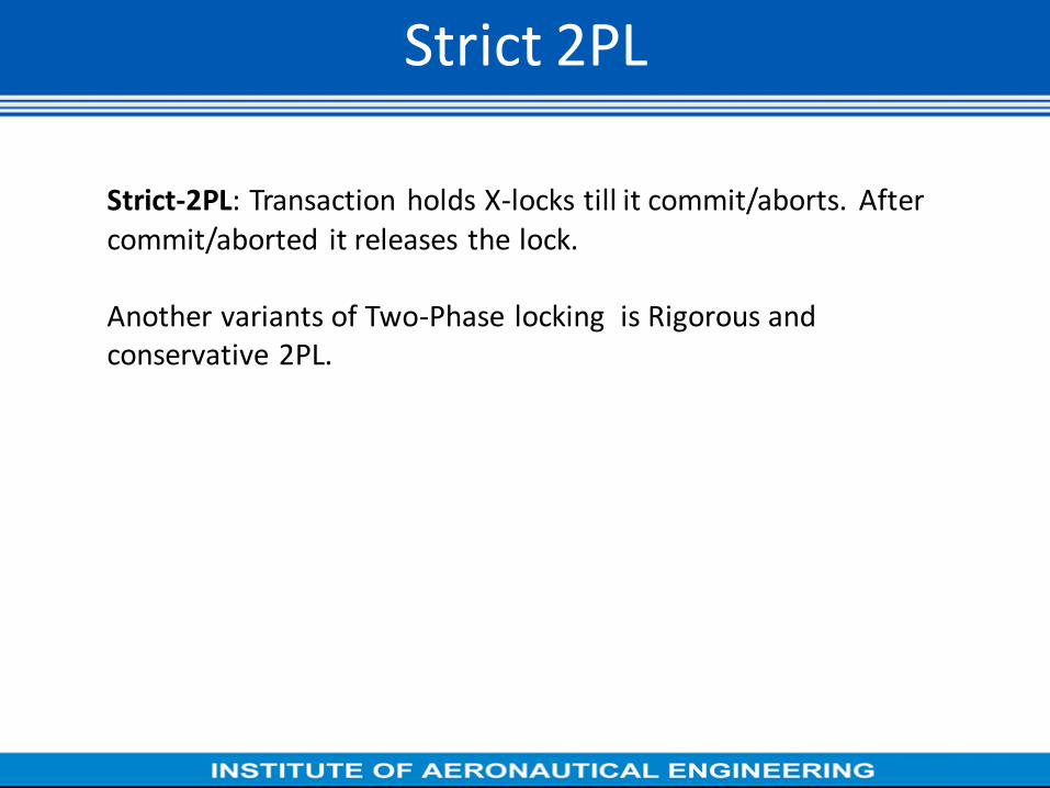
Strict 2PL
Strict-2PL: Transaction holds X-locks till it commit/aborts. After
commit/aborted it releases the lock.
Another variants of Two-Phase locking is Rigorous and
conservative 2PL.

variants of Two-Phase locking
Rigorous 2PL: T holds S|X locks till it commit |Aborts transactions can
be serialized in the order in which they commit.
Conservative 2PL:Transaction gets all locks in an atomic manner i.e. no
deadlocks.

Transaction Management
Time stamp based protocols

Timestamp Ordering
Timestamp:
– a number of generate by system.
– ticks of the computer's internal clock.
– no two transactions can have the same timestamp.

How timestamps are used ?
− A transaction Ti has time-stamp TS(Ti),
− A new transaction Tj is assigned time-stamp TS(Tj) such that
TS(Ti) <TS(Tj).

The protocol maintains for each data Q two timestamp values:
• W-timestamp(Q) is the largest time-stamp of any transaction that
executed write(Q) successfully.
• R-timestamp(Q) is the largest time-stamp of any transaction that
executed read(Q) successfully.

Timestamp-ordering Protocol
Case 1: Suppose that transaction Ti issues read(Q).
• If TS(Ti) ≤ W-timestamp(Q), then Ti needs to read a value of Q that
was already overwritten. Hence, Ti should read value before W-
timestamp. Therefore read operation is rejected, and Ti is rolled
back.
• If TS(Ti) W-timestamp(Q), then the read operation is executed,
and R-timestamp(Q) is set to max(R-timestamp(Q), TS(Ti)).Suppose
that transaction Ti issues write(Q).

Timestamp-ordering Protocol(contd.)
Case: 2 Suppose Ti issues write(Q).
• If TS(Ti) < R-timestamp(Q), since it has read-write conflict the write operation is rejected, and Ti is rolled back.
• If TS(Ti) < W-timestamp(Q), since it has write-write conflict the write operation is rejected, and Ti is rolled back. Otherwise, the write operation is executed, and W-timestamp(Q) is set to TS(Ti).
• If TS(Ti) > R-timestamp(Q) and TS(Ti) > W-timestamp(Q), since all read and write operations done before timestamp write operation is granted. Therefore w-timestamp need tobe updated with max of w-TS & TS(Ti).

Thomas’s write rule: • This rule states that if TS(Ti) < W-timestamp(Q) then the operation
is rejected & Ti is rolled back. Timestamp ordering rules can be
modified to make the schedule view serializable. Instead of making
Ti rolled back, the write operation itself is ignored.
Thomas’s write rule

Thomas’s write rule(contd.) Consider the given transactions
For the condition TS(Ti) < W-timestamp(Q) write of T2 is having largest
W-timestamp.
In case of T1 and T2 write operation is updated by W-timestamp(Q) to
TS(T1).
Under the thomas’s write rule, write(Q) on T1 would be ignored.

Transaction Management
Validation Based Protocol

Validation based protocol
Validation based protocol:
No checking is done while the transaction is executing.
Each transaction executes in three phases in its lifetime.
• Read phase: During this phase, the system executes transaction Ti It
reads the values of various data items and writes on temporary
local variables without updating the actual database.

Validation phases
• Validation phase: Transaction Ti performs a validation test to
determine the operation of read phase without violating the
serializability.
• Write phase: If Transaction Ti succeeds in validation then actual
updates are applied to the database otherwise the system rolls
back Ti.

Validation based protocol(contd.)
To perform the validation test, we need to know when the various phases of transaction Ti took place. Therefore associate three different timestamps with transaction Ti . The validation scheme is called as optimistic concurrency-control.
Three timestamps of validation are:
• Start (T): start of execution (Ti)
• Validation (T): Ti finished its read phase & started it validation phase.
• Finish (T): Time when Ti finished its write phase.
Serializability order by the timestamp-ordering technique is determined by using the value TS (Ti) = validation (Ti).

Validation Test
Validation Test:
For transaction TS(Ti) < TS(Ti), one of the following condition must hold
• Finish (Ti) < Start(Tj) : Since Ti completes its execution before Tj
started the serializability order is maintained.
• Start(Ti)< Finish (Ti) <Validation(Tj) :The validation phase of Tj
should occur after T i finishes.
• It ensures that writes of Ti & Tj do not overlap. Write (Ti) do not
effect read(Tj) hence serializability order is maintained.

Example for validating the transaction in a schedule

Transaction Management
Deadlock Handling

Deadlock Handling
• Consider the following two transactions:
T1: write (X) T2: write(Y)
write(Y) write(X)
• Schedule with deadlock

Deadlock Handling(contd.)
• System is deadlocked if there is a set of transactions such that
every transaction in the set is waiting for another transaction
in the set.
• Deadlock prevention protocols ensure that the system will
never enter into a deadlock state. Some prevention strategies
– Require that each transaction locks all its data items before
it begins execution (predeclaration).
– Impose partial ordering of all data items and require that a
transaction can lock data items only in the order specified
by the partial order (graph-based protocol).

Deadlock Prevention Strategies
• Following schemes use transaction timestamps for the sake of
deadlock prevention alone.
• wait-die scheme — non-preemptive
– older transaction may wait for younger one to release data
item. Younger transactions never wait for older ones; they are
rolled back instead.
– a transaction may die several times before acquiring needed
data item

Deadlock Prevention Strategies(contd.)
• wound-wait scheme — preemptive
– older transaction wounds (forces rollback) of younger
transaction instead of waiting for it. Younger transactions may
wait for older ones.
– may be fewer rollbacks than wait-die scheme.

Deadlock prevention (Cont.)
• Both in wait-die and in wound-wait schemes, a rolled back
transactions is restarted with its original timestamp. Older
transactions thus have precedence over newer ones, and starvation
is hence avoided.
• Timeout-Based Schemes :
– a transaction waits for a lock only for a specified amount of
time. After that, the wait times out and the transaction is rolled
back.
– thus deadlocks are not possible
– simple to implement; but starvation is possible. Also difficult to
determine good value of the timeout interval.

Deadlock Detection
• Deadlocks can be described as a wait-for graph, which consists of a
pair G = (V,E),
– V is a set of vertices (all the transactions in the system)
– E is a set of edges; each element is an ordered pair Ti Tj.
• If Ti Tj is in E, then there is a directed edge from Ti to Tj, implying
that Ti is waiting for Tj to release a data item.

Deadlock Detection( contd.)
• When Ti requests a data item currently being held by Tj, then the
edge Ti Tj is inserted in the wait-for graph. This edge is removed
only when Tj is no longer holding a data item needed by Ti.
• The system is in a deadlock state if and only if the wait-for graph
has a cycle. Must invoke a deadlock-detection algorithm
periodically to look for cycles.
Wait-for graph without a cycle Wait-for graph with a cycle

Deadlock Recovery
• When deadlock is detected :
– Some transaction will have to rolled back (made a victim) to
break deadlock. Select that transaction as victim that will incur
minimum cost.
– Rollback -- determine how far to roll back transaction
• Total rollback: Abort the transaction and then restart it.
• More effective to roll back transaction only as far as
necessary to break deadlock.
– Starvation happens if same transaction is always chosen as
victim. Include the number of rollbacks in the cost factor to
avoid starvation

Recovery System,
Recovery and Atomicity

Recovery System
Recovery system is an integral part of database management system
that can restore the database to the consistent state before failure.
The failures are categorized as failure that does not result in loss of
information and effects with loss of information.

Failures Failures are classified as:
1. Transaction failure The transaction may fail due to two errors. They are:
Logical error: The transaction further cannot continue with normal execution because of internal conditions as data not found, invalid input data, overflow or exceeded resource limits.
System error: The transaction further cannot continue with undesirable state like deadlock conditions.
2. System crash: System crash causes loss of the content of volatile storage. The reasons for this are: hardware problem; bug in the software or database software.
3. Disk failure: Disk crash leads to loss of information, which is due to failure due to data transfer or head crash. To recover from this failure backup on other disks, tapes.

Recovery from failure
The steps to determine how to recover from failures are:
• Identify the failure modes of storage devices.
• Consider how these failure modes effect the content of the
database
• Propose recovery algorithms to ensure DB properties such as
consistency, atomicity and durability. These algorithms has two
parts: To ensure recovery from failures; Action taken after a failure
to ensure DB properties.

Storage Structure
The storage types are defines by their relative speed, capacity and
resistance to failure. Broadly classified as volatile, nonvolatile and
stable storage.
• Volatile storage: The data in these storage cannot survive from
system crashes. Example as main and cache memory. Access to data
in volatile memory is fast and directly can access.
• Nonvolatile storage: It survives from system crashes. Example as
disk and magnetic tapes. The data in this leads to failure due to disk
crash, it leads to loss of data.
• Stable storage: Stable storage is impossible theoretically.

Stable storage implementation
• The implementation of stable storage requires:
• The replicate of data in several nonvolatile storage (disk) with
independent failure modes. Which is possible with RAID systems.
• Update the data in a controlled manner to ensure failure during
data transfer does not damage the required data. Block transfer
from storage to memory can be result any of these cases:
• Successful completion: Transfer of data without loss.
• Partial failure: A transfer at mid of transaction, it leads to incorrect
information at destination.
• Total failure: The failure occurred at early stage of transfer. Hence
no loss of data at destination block.

Recovery Process- Data transfer
To restore the data block to a consistent state during failure at data transfer requires:
• The storage system with two physical blocks for each logical database block. This can be done in two ways:
– Mirrored disks, if both are at the same location;
– Remote backup, if one is at local and other is at a remote site.
• The output operation is executed as: – Write the data onto the first physical block
– When first write completes successfully, write the same on the second disk.
– The output is completed only after the second write completes successfully.
– During Recovery the systems need to examine each pair of physical blocks and perform the require actions to ensure a successful write operation on stable storage or no change.

Actions required at different failures
Failure cases Actions required
Both blocks have same content
and no errors
No further actions required
Error in one block It replaces with content of other
block
Both blocks has no error, but the
content is different
The value of second block replace
with first block

Recovery procedure
Example: Let consider,
• Initially A and B have ₹1000 and ₹2000. The transaction Ti that transfers ₹50 from account A to account B;
• Goal is either to perform all database modifications made by Ti or none at all. Several output operations may be required for Ti (to output A and B).
• A failure may occur after one of these modifications have been made but before all of them are made.
The two possible recovery procedures are:
• Reexecute Ti : The system will enter into inconsistent state. It results the A with ₹900 instead of ₹950.
• Do not reexecute Ti : The system will enter into inconsistent state. The current system state has A with ₹900 and B with ₹2000.

Atomocity
• Modifying the database without ensuring that the transaction will
commit may leave the database in an inconsistent state.
• To ensure atomicity despite failures, we first output information
describing the modifications to stable storage without modifying
the database itself.

Recovery from failure
Two approaches for recovery:
• Log-based recovery
• Shadow-paging
Assume (initially) that transactions run serially, that is,
one after the other.

Recovery Algorithms
• Recovery algorithms are techniques to ensure database consistency
and transaction atomicity and durability even with failures.
Recovery algorithms have two parts:
• Actions taken during normal transaction processing to ensure
enough information exists to recover from failures
• Actions taken after a failure to recover the database contents to a
state that ensures atomicity, consistency and durability.
Two approaches using logs
• Deferred database modification
• Immediate database modification

Log-Based Recovery A log is kept on stable storage.
The log is a sequence of log records, and maintains a record of update
activities on the database.
Log record has 3 fields:
Transaction Identifier: Unique identifier of the transaction that
performed write operation.
Data item identifier: Unique identification of the data item written
Old value: Value of the item prior to the write
New value: Value of the item after write transaction

Cont..
Various log records are:
<Ti start> log record Before Ti executes write(X),
<Ti, X, V1, V2> is written, where V1 is the value of X before the write,
and V2 is the value to be written to X. Log record notes that Ti has
performed a write on data item Xj Xj had value V1 before the write,
and will have value V2 after the write.
<Ti commit> Transaction Ti has committed
<Ti abort> Transaction Ti has aborted

Deferred Database Modification The deferred database modification scheme records all modifications to the log, but
defers all the writes to after partial commit.
Assume that transactions execute serially.
<Ti start>transaction Ti started.
write(X) operation results in a log record :
<Ti, X, V> where V is the new value for X
Note: old value is not needed for this scheme
The write is not performed on X at this time, but is deferred.
When Ti partially commits,
<Ti commit> is written to the log
Finally, the log records are read and used to actually execute the previously deferred
writes. During recovery after a crash, a transaction needs to be redo if and only if both
<Ti start> and<Ti commit> are there in the log.
Redoing a transaction Ti
< redoTi> sets the value of all data items updated by the transaction to the new values.

Example
• Crashes can occur while the transaction is
executing the original updates, or while
recovery action is being taken example
transactions T0 and T1 (T0 executes before
T1):
• Let T0 be a transaction that transfers ₹50 from Account A to B. T1 be a transaction
that withdraws ₹100 from Account C. Initially A, B and C have ₹1000, ₹2000 and ₹700 respectively.
T0:
read (A)
A: - A - 50
Write(A)
read (B)
B:- B + 50
write (B)
T1 :
read (C)
C:-C- 100
write (C)

Log Record entries
Portion of database
log for T0 and T1
Log database
<T0 start>
<T0, A, 950>
<T0, B, 2050>
<T0, commit>
<T1 start>
<T1, C, 600>
<T1, commit>
< T0 start>
< T0, A, 950>
< T0, B, 2050>
< T0, commit>
<T1, start>
< T1, C, 600>
< T1,commit>
A=950
B=2050
C=600

Log updates at three instances of time
(a) (b) ( c)
<T0 start>
<T0, A, 950>
<T0, B, 2050>
< T0 start>
< T0, A, 950>
< T0, B, 2050>
< T0, commit>
<T1, start>
< T1, C, 600>
< T0 start>
< T0, A, 950>
< T0, B, 2050>
< T0, commit>
<T1, start>
< T1, C, 600>
< T1,commit>

Recovery actions
Case 1:
Shown in (a)
Crash occurs just after log
record for Write(B) of
transaction T0.
No redo action required due to no commit
in log.
The accounts A and B remains with initial
values.
Incomplete transaction T0 can be deleted
from the log
Case 2:
Shown in (b)
Crash occurs just after log
record for Write(C) of
transaction T1.
Redo(T0) is performed due to commit
record (<T0, commit>) in log.
The accounts A and B has with ₹950 and ₹2050 respectively.
Incomplete transaction T1 can be deleted
from the log
Case 3:
Shown in (c)
Crash occurs just after log
record (<T1, commit>) is
written in stable storage.
The accounts A, B and C has with ₹950, ₹2050 and ₹600 respectively.

Immediate Database Modification
• The immediate database modification scheme allows database
updates of an uncommitted transaction to be made as the writes are
issued since undoing may be needed, update logs must have both old
value and new value. Update log record must be written before
database item is written. Assume that the log record is output directly
to stable storage can be extended to postpone log record output, so
long as prior to execution of an output(B) operation for a data block
B, all log records corresponding to items B must be flushed to stable
storage.
• Output of updated blocks can take place at any time before or after
transaction commit
• Order in which blocks are output can be different from the order in
which they are written.

Recovery procedure operations
Recovery procedure has two operations instead of one:
• undo(Ti) restores the value of all data items updated by Ti to their
old values, going backwards from the last log record for Ti
• redo(Ti) sets the value of all data items updated by Ti to the new
values, going forward from the first log record for Ti
• Transaction Ti needs to be undone if the log contains the record
• <Ti start>, but does not contain the record <Ti commit>.
• Transaction Ti needs to be redone if the log contains both the
record <Ti start> and the record <Ti commit>.
Undo operations are performed first, then redo operations.

Example
• Let accounts A, B and C initially has ₹1000, ₹2000 and ₹700 respectively. The log entry of both the transactions are:
Log Database
<T0 start>
<T0, A, 1000, 950>
<To, B, 2000, 2050>
A = 950
B = 2050
<T0 commit>
<T1 start>
<T1, C, 700, 600>
C = 600
<T1 commit>

Cont..
• Using the log, the system can handle any failure that result in the loss of information in nonvolatile storage. Generally the recovery scheme uses any of two procedures:
• Undo (Ti) restores to old values.
• Redo (Ti) sets the updated values by transaction Ti to the new values.
• The set of data items updated by transaction Ti and respective new and old values are found in log. After failure occurs the recovery team consults the log to perform redo and undo operations on respective transactions.
• Undo (Ti) is performed, if the log contains <Ti start> but not contain <Ti commit>.
• Redo (Ti) is performed, if the log contains <Ti start> and <Ti commit>.

Failure
time slots
(a) (b) ( c)
Log <T0 start>
<T0, A, 1000, 950>
<To, B, 2000, 2050>
<T0 start>
<T0, A, 1000, 950>
<To, B, 2000, 2050>
<T0 commit>
<T1 start>
<T1, C, 700, 600>
<T0 start>
<T0, A, 1000, 950>
<To, B, 2000, 2050>
<T0 commit>
<T1 start>
<T1, C, 700, 600>
<T1 commit>
Recovery
Scheme
Undo(T0) Redo(T0)
Undo(T0)
Redo(T0)
Redo(T1)
Recovery
Action
Account A and B with
₹1000 and ₹2000
Account A, B and C
with ₹950, ₹2050 and
₹700.
Account A, B and C with
₹950, ₹2050 and₹ 600.
Recovery Actions

Example
• Crashes can occur while the transaction is
executing the original updates, or while
recovery action is being taken example
transactions T0 and T1 (T0 executes before
T1):
• Let T0 be a transaction that transfers ₹50 from Account A to B. T1 be a transaction
that withdraws ₹100 from Account C. Initially A, B and C have ₹1000, ₹2000 and ₹700 respectively.
T0:
read (A)
A: - A - 50
Write(A)
read (B)
B:- B + 50
write (B)
T1 :
read (C)
C:-C- 100
write (C)

Log Record entries
Portion of database
log for T0 and T1
Log database
<T0 start>
<T0, A, 950>
<T0, B, 2050>
<T0, commit>
<T1 start>
<T1, C, 600>
<T1, commit>
< T0 start>
< T0, A, 950>
< T0, B, 2050>
< T0, commit>
<T1, start>
< T1, C, 600>
< T1,commit>
A=950
B=2050
C=600
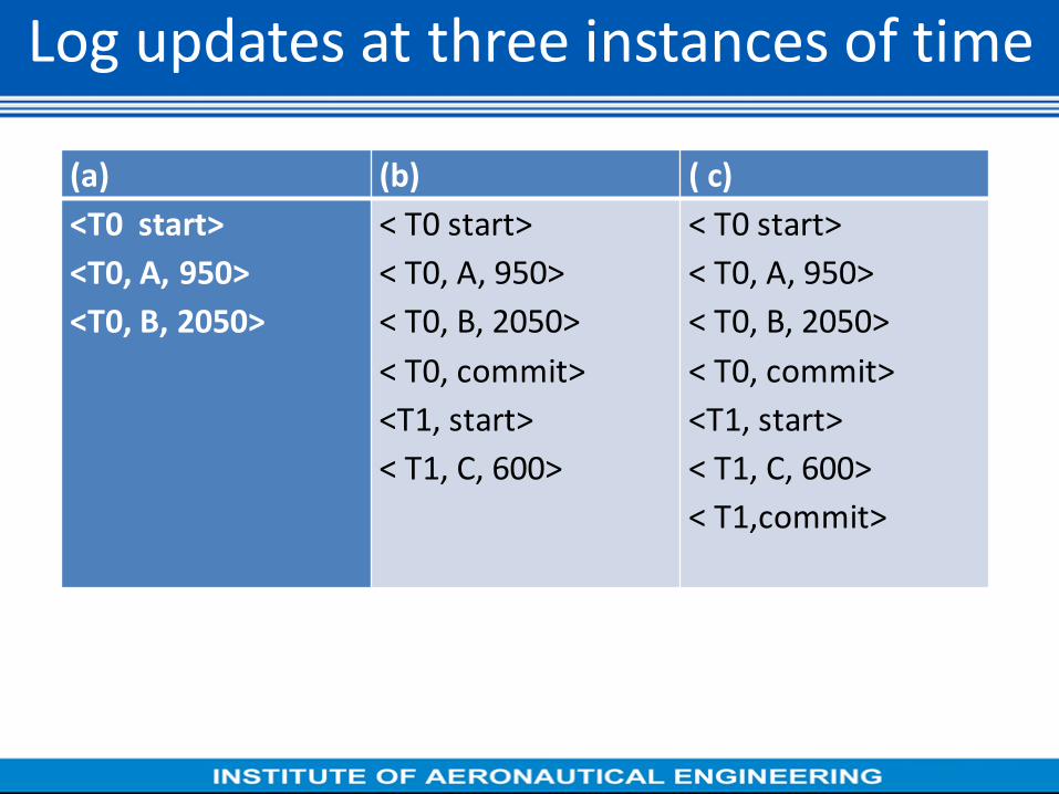
Log updates at three instances of time
(a) (b) ( c)
<T0 start>
<T0, A, 950>
<T0, B, 2050>
< T0 start>
< T0, A, 950>
< T0, B, 2050>
< T0, commit>
<T1, start>
< T1, C, 600>
< T0 start>
< T0, A, 950>
< T0, B, 2050>
< T0, commit>
<T1, start>
< T1, C, 600>
< T1,commit>
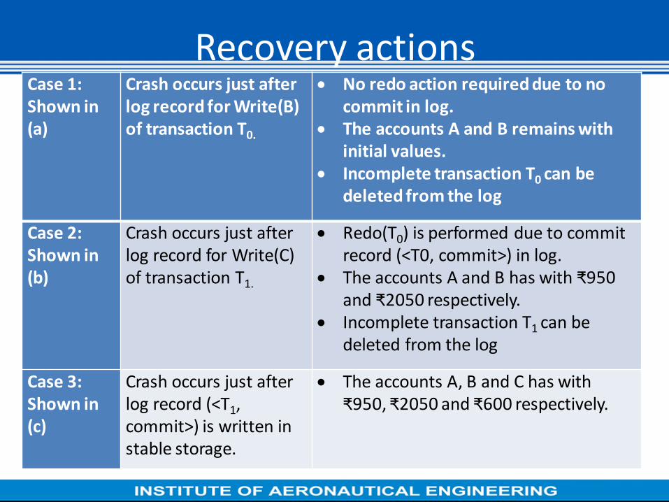
Recovery actions Case 1:
Shown in
(a)
Crash occurs just after
log record for Write(B)
of transaction T0.
No redo action required due to no
commit in log.
The accounts A and B remains with
initial values.
Incomplete transaction T0 can be
deleted from the log
Case 2:
Shown in
(b)
Crash occurs just after
log record for Write(C)
of transaction T1.
Redo(T0) is performed due to commit
record (<T0, commit>) in log.
The accounts A and B has with ₹950 and ₹2050 respectively.
Incomplete transaction T1 can be
deleted from the log
Case 3:
Shown in
(c)
Crash occurs just after
log record (<T1,
commit>) is written in
stable storage.
The accounts A, B and C has with
₹950, ₹2050 and ₹600 respectively.

Why check points required?
• Difficulties with Deferred and immediate database updates are
• The search process in time consuming
• Most of times the redo() need to be performed on already updated
data. With redo no harm, but it will cause recovery to take longer.
• To reduce the above said overheads, checkpoints are introduced.

Check points
Along with the system maintained log files using any of the two
techniques(deferred and Immediate), periodically performs the
checkpoints. Which requires the following sequence of actions:
• Output all log records from main memory to stable storage.
• Output to the disk all modified buffer blocks
• Output onto stable storage a log record <checkpoint>

Example
• Example: Let T1, T2, T3, and T4 are transaction recorded in log. Tc is
checkpoint and Tt is the failure occurred.

Steps to perform checkpoints
During recovery we need to consider only the most recent transaction Ti that started before the checkpoint, and transactions that started after Ti.
1. Scan backwards from end of log to find the most recent <checkpoint> record
2. Continue scanning backwards till a record <Ti start> is found.
3. Need only consider the part of log following above start record. Earlier part of log can be ignored during recovery, and can be erased whenever desired.
4. For all transactions (starting from Ti or later) with no <T i commit>, execute undo(Ti). (Done only in case of immediate modification.)
5. Scanning forward in the log, for all transactions starting from Ti or later with a <Ti commit>, execute redo(Ti).

Shadow paging
Shadow paging is an alternative to log-based recovery; this scheme is useful if transactions execute serially
• Maintain two page tables during the lifetime of a transaction –the current page table, and the shadow page table.
• Store the shadow page table in nonvolatile storage, such that state of the database prior to transaction execution may be recovered. Shadow page table is never modified during execution.
• To start with, both the page tables are identical. Only current page table is used for data item accesses during execution of the transaction.
• Whenever any page is about to be written for the first time:
• Copy of this page is made onto an unused page.
• Current page table is then made to point to the copy.
• Update is performed on the copy

Example of Shadow paging

Steps to commit a transaction
To commit a transaction : 1. Flush all modified pages in main memory to disk
2. Output current page table to disk
3. Make the current page table the new shadow page table, as follows:
• keep a pointer to the shadow page table at a fixed (known) location on disk.
• to make the current page table the new shadow page table, simply update the pointer to point to current page table on disk
• Once pointer to shadow page table has been written, transaction is committed.
• No recovery is needed after a crash — new transactions can start right away, using the shadow page table.
• Pages not pointed to from current/shadow page table should be freed (garbage collected).

Advantages
• Advantages of shadow-paging over log-based schemes
– no overhead of writing log records
– recovery is trivial
• Disadvantages
• Copying the entire page table is very expensive
• Need to flush every updated page, and page table
• Need to flush every updated page, and page table

Disadvantages
– Copying the entire page table is very expensive
– Can be reduced by using a page table structured like a B+-tree
– No need to copy entire tree, only need to copy paths in the tree that lead to updated leaf nodes
– Commit overhead is high even with above extension
– Need to flush every updated page, and page table
– Data gets fragmented (related pages get separated on disk)
– After every transaction completion, the database pages containing old versions of modified data need to be garbage collected
– Hard to extend algorithm to allow transactions to run concurrently
• Easier to extend log based schemes

Recovery actions Case 1:
Shown in
(a)
Crash occurs just after
log record for Write(B)
of transaction T0.
No redo action required due to no
commit in log.
The accounts A and B remains with
initial values.
Incomplete transaction T0 can be
deleted from the log
Case 2:
Shown in
(b)
Crash occurs just after
log record for Write(C)
of transaction T1.
Redo(T0) is performed due to commit
record (<T0, commit>) in log.
The accounts A and B has with ₹950 and ₹2050 respectively.
Incomplete transaction T1 can be
deleted from the log
Case 3:
Shown in
(c)
Crash occurs just after
log record (<T1,
commit>) is written in
stable storage.
The accounts A, B and C has with
₹950, ₹2050 and ₹600 respectively.

UNIT - V
DATA STORAGE AND QUERY PROCESSING

Physical Storage Media, Magnetic disks
Physical Storage Media Cache – fastest and most costly form of storage; volatile; managed by
the computer system hardware.
Main memory --fast access (10s to 100s of nanoseconds; 1 nanosecond
= 10–9 seconds)
generally too small (or too expensive) to store the entire database
Capacities of up to a few Gigabytes widely used currently
Capacities have gone up and per-byte costs have decreased steadily and
rapidly (roughly factor of 2 every 2 to 3 years)
Volatile: contents of main memory are usually lost if a power failure or
system crash occurs.
Flash memory :Data survives power failure

Classification of Physical Storage Media
•Speed with which data can be accessed
•Cost per unit of data
•Reliability
data loss on power failure or system crash
physical failure of the storage device
•Can differentiate storage into:
volatile storage: loses contents when power is switched off
non-volatile storage:
l Contents persist even when power is switched off.
lI Includes secondary and tertiary storage, as well as batter-
backed up main-memory.

Magnetic-disk
• Data is stored on spinning disk, and read/written magnetically
• Primary medium for the long-term storage of data; typically
stores entire database.
• Data must be moved from disk to main memory for access, and
written back for storage
• Much slower access than main memory (more on this later)
• direct-access – possible to read data on disk in any order,
unlike magnetic tape
• Capacities range up to roughly 1.5 TB as of 2009
• Much larger capacity and cost/byte than main memory/flash
memory
• Growing constantly and rapidly with technology improvements
(factor of 2 to 3 every 2 years)
• Survives power failures and system crashes

Optical storage
• Non-volatile, data is read optically from a spinning disk using a laser
• CD-ROM (640 MB) and DVD (4.7 to 17 GB) most popular forms
• Blu-ray disks: 27 GB to 54 GB
• Write-one, read-many (WORM) optical disks used for archival storage
(CD-R, DVD-R, DVD+R)
• Multiple write versions also available
(CD-RW, DVD-RW, DVD+RW, and DVD-RAM)
• Reads and writes are slower than with magnetic disk
• Juke-box systems, with large numbers of removable disks, a few drives, and a mechanism for automatic loading/unloading of disks available for storing large volumes of data

Tape storage
• Non-volatile, used primarily for backup (to recover from disk failure),
and for archival data
• sequential-access – much slower than disk
• very high capacity (40 to 300 GB tapes available)
• tape can be removed from drive storage costs much cheaper than
disk, but drives are expensive

Storage Hierarchy
Primary storage: Fastest media but
volatile (cache, main memory).
Secondary storage: next level in
hierarchy, non-volatile, moderately
fast access time also called on-line
storage
E.g. flash memory, magnetic disks
Tertiary storage: lowest level in
hierarchy, non-volatile, slow access
time also called off-line storage
E.g. magnetic tape, optical storage

RAID
RAID: Redundant Arrays of Independent Disks • RAID id a disk organization techniques that manage a large numbers
of disks, providing a view of a single disk of
• high capacity and high speed by using multiple disks in parallel,
• high reliability by storing data redundantly, so that data can be
recovered even if a disk fails

RAID Levels
• RAID Level 0: Block striping; non-redundant.
– Used in high-performance applications where data loss is not critical.
• RAID Level 2: Memory-Style Error-Correcting-Codes (ECC) with bit striping.
• RAID Level 3: Bit-Interleaved Parity
• RAID Level 4: Block-Interleaved Parity;
uses block-level striping, and keeps a parity block on a separate disk for corresponding blocks from N other disks.
• RAID Level 5: Block-Interleaved Distributed Parity;
partitions data and parity among all N + 1 disks, rather than storing data in N disks and parity in 1 disk.

RAID Levels

Factors in choosing RAID level
• Monetary cost
• Performance: Number of I/O operations per second, and bandwidth
during normal operation
• Performance during failure
• Performance during rebuild of failed disk
• Including time taken to rebuild failed disk

File organization Techniques
•The database is stored as a collection of files.
•Each file is a sequence of records.
• A record is a sequence of fields.
•Fixed Length Record
•Variable Length Record
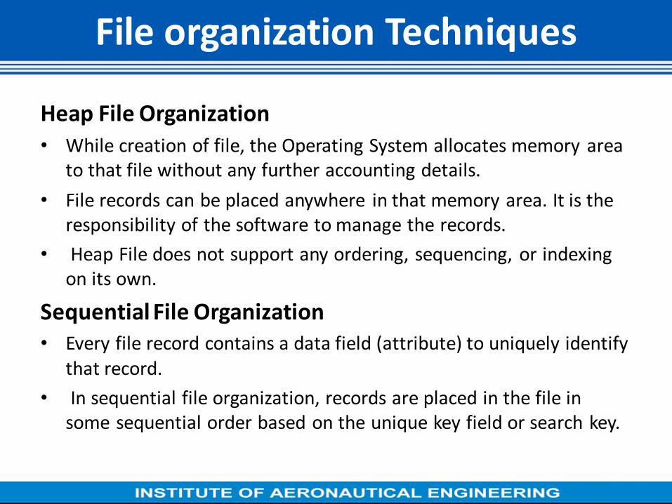
File organization Techniques
Heap File Organization
• While creation of file, the Operating System allocates memory area
to that file without any further accounting details.
• File records can be placed anywhere in that memory area. It is the
responsibility of the software to manage the records.
• Heap File does not support any ordering, sequencing, or indexing
on its own.
Sequential File Organization
• Every file record contains a data field (attribute) to uniquely identify
that record.
• In sequential file organization, records are placed in the file in
some sequential order based on the unique key field or search key.

File organization Techniques
Hash File Organization
• Uses Hash function computation on some fields of the records.
• The output of the hash function determines the location of disk
block where the records are to be placed.
Clustered File Organization
• Not considered good for large databases
• Related records from one or more relations are kept in the same
disk block, i.e. the ordering of records is not based on primary key
or search key.

Sequential File Organization
•Suitable for applications that require
sequential processing of the entire file
•The records in the file are ordered by
a search-key.
Insertion –locate the position where
the record is to be inserted
• if there is free space insert there
• if no free space, insert the record
in an overflow block
•In either case, pointer chain must
be updated
•Need to reorganize the file from
time to time to restore sequential
order

Multitable Clustering File Organization
• Store several relations in one file using a multitable clustering file
organization
department
instructor
Multitable clustering of department and instructor

Record organization Techniques
Fixed-Length Records
Store record i starting from byte n (i – 1), where n is the size of each
record.
Record access is simple but records may cross blocks
Modification: do not allow records to cross block boundaries
Deletion of record i: alternatives:
move records i + 1, . . ., n to i, . . . , n – 1 move record n to ido not
move records, but link all free records on a free list

Deleting record 3 and compacting

Free Lists
• Store the address of the first deleted record in the file header.
• Use this first record to store the address of the second deleted record, and so on
• Can think of these stored addresses as pointers since they “point” to the location of a record.
• More space efficient representation: reuse space for normal attributes of free records to store pointers. (No pointers stored in in-use records.)

Variable-Length Records
• Variable-length records arise in database systems in several ways:
• Storage of multiple record types in a file.
• Record types that allow variable lengths for one or more fields such
as strings (varchar)
• Record types that allow repeating fields (used in some older data
models).
• Attributes are stored in order
• Variable length attributes represented by fixed size (offset, length),
with actual data stored after all fixed length attributes
• Null values represented by null-value bitmap

Basic Concepts :Indexing
Structures for Files - Different
types of Indices

Ordered Indices
In an ordered index, index entries are stored sorted on the search key
value. E.g., author catalog in library.
Primary index: in a sequentially ordered file, the index whose search key
specifies the sequential order of the file,Also called clustering index
The search key of a primary index is usually but not necessarily the primary
key.
Secondary index: an index whose search key specifies an order different from
the sequential order of the file. Alsocalled non-clustering index.
Index-sequential file: ordered sequential file with a primary index.

Dense Index Files
• Dense index — Index record appears for every search-key value
in the file.
• E.g. index on ID attribute of instructor relation

Basic Concepts
• Indexing mechanisms used to speed up access to desired data.
– E.g., author catalog in library
• Search Key - attribute to set of attributes used to look up records in a
file.
• An index file consists of records (called index entries) of the form
• Index files are typically much smaller than the original file
• Two basic kinds of indices:
– Ordered indices: search keys are stored in sorted order
– Hash indices: search keys are distributed uniformly across “buckets” using a “hash function”.

Index Evaluation Metrics
• Access types supported efficiently. E.g.,
– records with a specified value in the attribute
– or records with an attribute value falling in a specified range of
values.
• Access time
• Insertion time
• Deletion time
• Space overhead

Ordered Indices
• In an ordered index, index entries are stored sorted on the search key
value. E.g., author catalog in library.
• Primary index: in a sequentially ordered file, the index whose search key
specifies the sequential order of the file.
– Also called clustering index
– The search key of a primary index is usually but not necessarily the
primary key.
• Secondary index: an index whose search key specifies an order different
from the sequential order of the file. Also called
non-clustering index.
• Index-sequential file: ordered sequential file with a primary index.

Dense Index Files
• Dense index — Index record appears for every search-key value in the
file.
• E.g. index on ID attribute of instructor relation

Dense Index Files (Cont.)
• Dense index on dept_name, with instructor file sorted on dept_name

Sparse Index Files
• Sparse Index: contains index records for only some search-key values.
– Applicable when records are sequentially ordered on search-key
• To locate a record with search-key value K we:
– Find index record with largest search-key value < K
– Search file sequentially starting at the record to which the index
record points

Sparse Index Files (Cont.)
• Compared to dense indices:
– Less space and less maintenance overhead for insertions and
deletions.
– Generally slower than dense index for locating records.
• Good tradeoff: sparse index with an index entry for every block
in file, corresponding to least search-key value in the block.

Secondary Indices Example
Secondary index on salary field of instructor
• Index record points to a bucket that contains pointers to all the actual
records with that particular search-key value.
• Secondary indices have to be dense

Primary and Secondary Indices
• Indices offer substantial benefits when searching for records.
• BUT: Updating indices imposes overhead on database modification --
when a file is modified, every index on the file must be updated,
• Sequential scan using primary index is efficient, but a sequential scan
using a secondary index is expensive
– Each record access may fetch a new block from disk
– Block fetch requires about 5 to 10 milliseconds, versus about 100
nanoseconds for memory access

Multilevel Index
• If primary index does not fit in memory, access becomes expensive.
• Solution: treat primary index kept on disk as a sequential file and
construct a sparse index on it.
– outer index – a sparse index of primary index
– inner index – the primary index file
• If even outer index is too large to fit in main memory, yet another level
of index can be created, and so on.
• Indices at all levels must be updated on insertion or deletion from the
file.

Multilevel Index (Cont.)

Index Update: Deletion
If deleted record was the only record in the file with its particular
search-key value, the search-key is deleted from the index also.
• Single-level index entry deletion:
– Dense indices – deletion of search-key is similar to file record
deletion.
– Sparse indices –
• if an entry for the search key exists in the index, it is deleted by
replacing the entry in the index with the next search-key value
in the file (in search-key order).
• If the next search-key value already has an index entry, the entry
is deleted instead of being replaced.

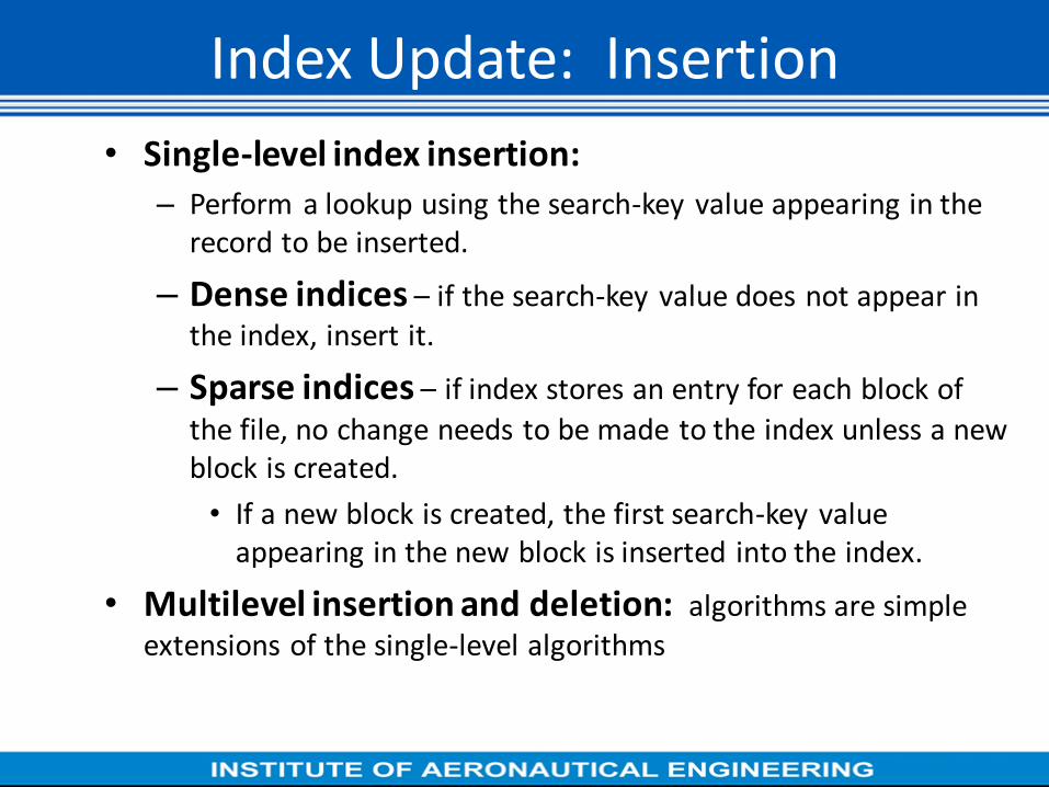
Index Update: Insertion
• Single-level index insertion:
– Perform a lookup using the search-key value appearing in the
record to be inserted.
– Dense indices – if the search-key value does not appear in
the index, insert it.
– Sparse indices – if index stores an entry for each block of
the file, no change needs to be made to the index unless a new
block is created.
• If a new block is created, the first search-key value
appearing in the new block is inserted into the index.
• Multilevel insertion and deletion: algorithms are simple
extensions of the single-level algorithms

Secondary Indices
• Frequently, one wants to find all the records whose
values in a certain field (which is not the search-key of the
primary index) satisfy some condition.
– Example 1: In the instructor relation stored sequentially
by ID, we may want to find all instructors in a particular
department
– Example 2: as above, but where we want to find all
instructors with a specified salary or with salary in a
specified range of values
• We can have a secondary index with an index record for each
search-key value

Other Features
• Covering indices
– Add extra attributes to index so (some) queries can avoid
fetching the actual records
• Particularly useful for secondary indices
– Why?
– Can store extra attributes only at leaf

B-TREES INDEXED FILE

B-tree
• Index structures for large datasets cannot be stored in main
memory
• Storing it on disk requires different approach to efficiency
• Assuming that a disk spins at 3600 RPM, one revolution occurs in
1/60 of a second, or 16.7ms
• Crudely speaking, one disk access takes about the same time as
200,000 instructions

Motivation (cont.)
• Assume that we use an AVL tree to store about 20 million records
• We end up with a very deep binary tree with lots of different disk
accesses; log2 20,000,000 is about 24, so this takes about 0.2 seconds
• We know we can’t improve on the log n lower bound on search for a
binary tree
• But, the solution is to use more branches and thus reduce the height
of the tree!
– As branching increases, depth decreases
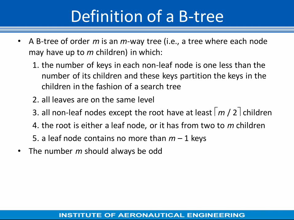
Definition of a B-tree
• A B-tree of order m is an m-way tree (i.e., a tree where each node
may have up to m children) in which:
1. the number of keys in each non-leaf node is one less than the
number of its children and these keys partition the keys in the
children in the fashion of a search tree
2. all leaves are on the same level
3. all non-leaf nodes except the root have at least m / 2 children
4. the root is either a leaf node, or it has from two to m children
5. a leaf node contains no more than m – 1 keys
• The number m should always be odd

An example B-Tree
51 62 42
6 12
26
55
60
70
64
90
45
1 2 4 7 8 13 15 18 25
27
29
46
48
53
A B-tree of order 5
containing 26 items
Note that all the leaves are at the same level

Constructing a B-tree
• Suppose we start with an empty B-tree and keys arrive in the following order:1 12 8 2 25 5 14 28 17 7 52 16 48 68 3 26 29 53 55 45
• We want to construct a B-tree of order 5
• The first four items go into the root:
• To put the fifth item in the root would violate condition 5
• Therefore, when 25 arrives, pick the middle key to make a new root

Constructing a B-tree (contd.)
1 2
8
12 25
6, 14, 28 get added to the leaf nodes:
1 2
8
12 14 6 25 28

Constructing a B-tree (contd.)
• Adding 17 to the right leaf node would over-fill it, so we take the
middle key, promote it (to the root) and split the leaf
12 14 25 28 1 2 6
8 17
12 14 25 28 1 2 6
7, 52, 16, 48 get added to the leaf nodes
8 17
12 14 25 28 1 2 6 16 48 52 7

Constructing a B-tree (contd.)
• Adding 68 causes us to split the right most leaf, promoting 48
to the root, and adding 3 causes us to split the left most leaf,
promoting 3 to the root; 26, 29, 53, 55 then go into the leaves
3 8 17 48
52 53 55 68 25 26 28 29 1 2 6 7 12 14 16
Adding 45 causes a split of 25 26 28 29
and promoting 28 to the root then causes the root to split

• The maximum number of items in a B-tree of order m and height h: Root m – 1
level 1 m(m – 1)
level 2 m2(m – 1)
. . .
level h mh(m – 1)
• So, the total number of items is
(1 + m + m2 + m3 + … + mh)(m – 1) =
[(mh+1 – 1)/ (m – 1)] (m – 1) = mh+1 – 1
• When m = 5 and h = 2 this gives 53 – 1 = 124
Analysis of B-Trees

Reasons for using B-Trees
• When searching tables held on disc, the cost of each disc transfer is high but doesn't depend much on the amount of data transferred, especially if consecutive items are transferred – If we use a B-tree of order 101, say, we can transfer each node
in one disc read operation
– A B-tree of order 101 and height 3 can hold 1014 – 1 items (approximately 100 million) and any item can be accessed with 3 disc reads (assuming we hold the root in memory)
• If we take m = 3, we get a 2-3 tree, in which non-leaf nodes have two or three children (i.e., one or two keys) – B-Trees are always balanced (since the leaves are all at the same
level), so 2-3 trees make a good type of balanced tree

Comparing Trees
• Binary trees – Can become unbalanced and lose their good time complexity
(big O)
– AVL trees are strict binary trees that overcome the balance problem
– Heaps remain balanced but only prioritise (not order) the keys
• Multi-way trees – B-Trees can be m-way, they can have any (odd) number of
children
– One B-Tree, the 2-3 (or 3-way) B-Tree, approximates a permanently balanced binary tree, exchanging the AVL tree’s balancing operations for insertion and (more complex) deletion operations

B+-Tree Index Files
B+-tree indices are an alternative to indexed-sequential files.
• Disadvantage of indexed-sequential files
– performance degrades as file grows, since many overflow blocks get created.
– Periodic reorganization of entire file is required.
• Advantage of B+-tree index files:
– automatically reorganizes itself with small, local, changes, in the face of insertions and deletions.
– Reorganization of entire file is not required to maintain performance.
• (Minor) disadvantage of B+-trees:
– extra insertion and deletion overhead, space overhead.
• Advantages of B+-trees outweigh disadvantages
– B+-trees are used extensively
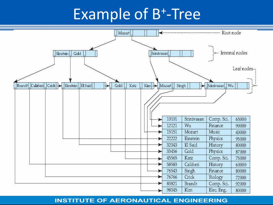
Example of B+-Tree

B+-Tree Index Files (Cont.)
:A B+-tree is a rooted tree satisfying the following properties
• All paths from root to leaf are of the same length
• Each node that is not a root or a leaf has between n/2 and n
children.
• A leaf node has between (n–1)/2 and n–1 values
• Special cases:
– If the root is not a leaf, it has at least 2 children.
– If the root is a leaf (that is, there are no other nodes in the
tree), it can have between 0 and (n–1) values.

B+-Tree Node Structure
• Typical node
– Ki are the search-key values
– Pi are pointers to children (for non-leaf nodes) or pointers to
records or buckets of records (for leaf nodes).
• The search-keys in a node are ordered
K1 < K2 < K3 < . . . < Kn–1
(Initially assume no duplicate keys, address duplicates later)

Leaf Nodes in B+-Trees
• For i = 1, 2, . . ., n–1, pointer Pi points to a file record with search-key
value Ki,
• If Li, Lj are leaf nodes and i < j, Li’s search-key values are less than or equal
to Lj’s search-key values
• Pn points to next leaf node in search-key order

Non-Leaf Nodes in B+-Trees
• Non leaf nodes form a multi-level sparse index on the leaf nodes.
For a non-leaf node with m pointers:
– All the search-keys in the subtree to which P1 points are less
than K1
– For 2 i n – 1, all the search-keys in the subtree to which Pi
points have values greater than or equal to Ki–1 and less than Ki
– All the search-keys in the subtree to which Pn points have values
greater than or equal to Kn–1

Example of B+-tree
B+-tree for instructor file (n = 6)
• Leaf nodes must have between 3 and 5 values ((n–1)/2 and n –1, with n = 6).
• Non-leaf nodes other than root must have between 3 and 6 children ((n/2 and n with n =6).
• Root must have at least 2 children.

Observations about B+-trees
• Since the inter-node connections are done by pointers, “logically” close blocks need not be “physically” close.
• The non-leaf levels of the B+-tree form a hierarchy of sparse indices.
• The B+-tree contains a relatively small number of levels
• Level below root has at least 2* n/2 values
• Next level has at least 2* n/2 * n/2 values
• .. etc.
– If there are K search-key values in the file, the tree height is no
more than logn/2(K) – thus searches can be conducted efficiently.
• Insertions and deletions to the main file can be handled efficiently,
as the index can be restructured in logarithmic time (as we shall
see).

Queries on B+-Trees
• Find record with search-key value V.
1. C=root
2. While C is not a leaf node {
1. Let i be least value s.t. V Ki.
2. If no such exists, set C = last non-null pointer in C
3. Else { if (V= Ki ) Set C = Pi +1 else set C = Pi}
}
3. Let i be least value s.t. Ki = V
4. If there is such a value i, follow pointer Pi to the desired record.
5. Else no record with search-key value k exists.

Queries on B+-Trees (Cont.) • If there are K search-key values in the file, the height of the tree is no
more than logn/2(K). • A node is generally the same size as a disk block, typically 4 kilobytes
– and n is typically around 100 (40 bytes per index entry).
• With 1 million search key values and n = 100
– at most log50(1,000,000) = 4 nodes are accessed in a lookup.
• Contrast this with a balanced binary tree with 1 million search key values
— around 20 nodes are accessed in a lookup
– above difference is significant since every node access may need a disk
I/O, costing around 20 milliseconds

B-Tree Index Files (Cont.)
• Advantages of B-Tree indices:
– May use less tree nodes than a corresponding B+-Tree.
– Sometimes possible to find search-key value before reaching leaf
node.
• Disadvantages of B-Tree indices:
– Only small fraction of all search-key values are found early
– Non-leaf nodes are larger, so fan-out is reduced. Thus, B-Trees
typically have greater depth than corresponding B+-Tree
– Insertion and deletion more complicated than in B+-Trees
– Implementation is harder than B+-Trees.
• Typically, advantages of B-Trees do not out weigh disadvantages.

Static Hashing Static Hashing
• A bucket is a unit of storage containing one or more records (a bucket
is typically a disk block).
• In a hash file organization we obtain the bucket of a record directly
from its search-key value using a hash function.
• Hash function h is a function from the set of all search-key values K to
the set of all bucket addresses B.
• Hash function is used to locate records for access, insertion as well as
deletion.
• Records with different search-key values may be mapped to the same
bucket; thus entire bucket has to be searched sequentially to locate a
record.

Example of Hash File Organization
Hash file organization of instructor file, using dept_name as key (See
figure in next slide.)
characters modulo 10
E.g. h(Music) = There are 10 buckets,
The binary representation of the ith character is assumed to be
the integer i.
The hash function returns the sum of the binary representations
of the 1 h(History) = 2
h(Physics) = 3 h(Elec. Eng.) = 3

Example of Hash File Organization
Hash file organization of instructor file, using dept_name as key
(see previous slide for details).

Hash Functions
• Worst hash function maps all search-key values to the same bucket; this
makes access time proportional to the number of search-key values in the
file.
• An ideal hash function is uniform, i.e., each bucket is assigned the same
number of search-key values from the set of all possible values.
• Ideal hash function is random, so each bucket will have the same number of
records assigned to it irrespective of the actual distribution of search-key
values in the file.
• Typical hash functions perform computation on the internal binary
representation of the search-key.
• For example, for a string search-key, the binary representations of all the
characters in the string could be added and the sum modulo the number of
buckets could be returned.

Handling of Bucket Overflows (Cont.)
• Overflow chaining – the overflow buckets of a given bucket are
chained together in a linked list.
• Above scheme is called closed hashing.
– An alternative, called open hashing, which does not use
overflow buckets, is not suitable for database applications.

Hash Indices
• Hashing can be used not only for file organization, but also for
index-structure creation.
• A hash index organizes the search keys, with their associated record
pointers, into a hash file structure.
• Strictly speaking, hash indices are always secondary indices
– if the file itself is organized using hashing, a separate primary
hash index on it using the same search-key is unnecessary.
– However, we use the term hash index to refer to both secondary
index structures and hash organized files.

Example of Hash Index

Deficiencies of Static Hashing
• In static hashing, function h maps search-key values to a fixed set of
B of bucket addresses. Databases grow or shrink with time.
– If initial number of buckets is too small, and file grows,
performance will degrade due to too much overflows.
– If space is allocated for anticipated growth, a significant amount
of space will be wasted initially (and buckets will be under full).
– If database shrinks, again space will be wasted.
• One solution: periodic re-organization of the file with a new hash
function
– Expensive, disrupts normal operations
• Better solution: allow the number of buckets to be modified
dynamically.

Dynamic Hashing
• Good for database that grows and shrinks in size
• Allows the hash function to be modified dynamically
• Extendable hashing – one form of dynamic hashing
– Hash function generates values over a large range — typically b-bit integers, with b = 32.
– At any time use only a prefix of the hash function to index into a table of bucket addresses.
– Let the length of the prefix be i bits, 0 i 32.
• Bucket address table size = 2i. Initially i = 0
• Value of i grows and shrinks as the size of the database grows and shrinks.
– Multiple entries in the bucket address table may point to a bucket (why?)
– Thus, actual number of buckets is < 2i
• The number of buckets also changes dynamically due to coalescing and splitting of buckets.

General Extendable Hash Structure
In this structure, i2 = i3 = i, whereas i1 = i – 1 (see
next slide for details)
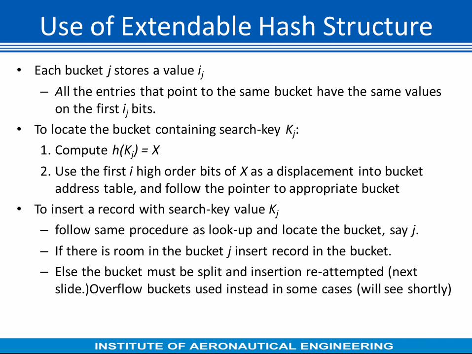
Use of Extendable Hash Structure
• Each bucket j stores a value ij
– All the entries that point to the same bucket have the same values
on the first ij bits.
• To locate the bucket containing search-key Kj:
1. Compute h(Kj) = X
2. Use the first i high order bits of X as a displacement into bucket
address table, and follow the pointer to appropriate bucket
• To insert a record with search-key value Kj
– follow same procedure as look-up and locate the bucket, say j.
– If there is room in the bucket j insert record in the bucket.
– Else the bucket must be split and insertion re-attempted (next
slide.)Overflow buckets used instead in some cases (will see shortly)

Insertion in Extendable Hash Structure(Cont)
To split a bucket j when inserting record with search-key
value Kj:
• If i > ij (more than one pointer to bucket j) – allocate a new bucket z, and set ij = iz = (ij + 1) – Update the second half of the bucket address table entries
originally pointing to j, to point to z
– remove each record in bucket j and reinsert (in j or z) – recompute new bucket for Kj and insert record in the bucket
(further splitting is required if the bucket is still full) • If i = ij (only one pointer to bucket j)
– If i reaches some limit b, or too many splits have happened in this insertion, create an overflow bucket
– Else • increment i and double the size of the bucket address table. • replace each entry in the table by two entries that point to
the same bucket. • recompute new bucket address table entry for Kj
Now i > ij so use the first case above.

Deletion in Extendable Hash Structure
• To delete a key value,
– locate it in its bucket and remove it.
– The bucket itself can be removed if it becomes empty (with
appropriate updates to the bucket address table).
– Coalescing of buckets can be done (can coalesce only with a
“buddy” bucket having same value of ij and same ij –1 prefix, if it
is present)
– Decreasing bucket address table size is also possible
• Note: decreasing bucket address table size is an expensive
operation and should be done only if number of buckets
becomes much smaller than the size of the table

Use of Extendable Hash Structure:
Example

Extendable Hashing vs. Other Schemes
• Benefits of extendable hashing: – Hash performance does not degrade with growth of file
– Minimal space overhead
• Disadvantages of extendable hashing
– Extra level of indirection to find desired record
– Bucket address table may itself become very big (larger than memory)Cannot allocate very large contiguous areas on disk either
– Solution: B+-tree structure to locate desired record in bucket address table Changing size of bucket address table is an expensive operation
• Linear hashing is an alternative mechanism
– Allows incremental growth of its directory (equivalent to bucket address table)At the cost of more bucket overflows

Comparison of Ordered Indexing
and Hashing • Cost of periodic re-organization
• Relative frequency of insertions and deletions
• Is it desirable to optimize average access time at the expense of
worst-case access time?
• Expected type of queries:
– Hashing is generally better at retrieving records having a
specified value of the key.
– If range queries are common, ordered indices are to be
preferred
• In practice:
– PostgreSQL supports hash indices, but discourages use due to
poor performance
– Oracle supports static hash organization, but not hash indices -
SQLServer supports only B+-trees

Dynamic Hashing
As the database grows over time, we have three options:
• - Choose hash function based on current file size. Get
• performance degradation as file grows.
• - Choose hash function based on anticipated file size.
• Space is wasted initially.
• -Periodically re-organize hash structure as file grows.
• Requires selecting new hash function, recomposing all
• addresses and generating new bucket assignments.
• Costly, and shuts down database.

• Some hashing techniques allow the hash function to be modified
dynamically to accommodate the growth or shrinking of the
database. These are called dynamic hash functions.Extendable
hashing is one form of dynamic hashing.
• Extendable hashing splits and coalesces buckets as database size
changes.
• This imposes some performance overhead, but space efficiency is
maintained.
• As reorganization is on one bucket at a time, overhead is acceptably
low.

General extendable hash structure.

• We choose a hash function that is uniform and random that generates values over a relatively large range.
• Range is b-bit binary integers (typically b=32).
• is over 4 billion, so we don't generate that many buckets!
• Instead we create buckets on demand, and do not use all b bits of the hash initially.
• At any point we use i bits where .
• The i bits are used as an offset into a table of bucket addresses.
• Value of i grows and shrinks with the database.
• Figure shows an extendable hash structure.
• Note that the i appearing over the bucket address table tells how many bits are required to determine the correct bucket.
• It may be the case that several entries point to the same bucket.
• All such entries will have a common hash prefix, but the length of this prefix may be less than i.
• So we give each bucket an integer giving the length of the common hash prefix.
• This is shown in Figure in the before slide as .
• Number of bucket entries pointing to bucket j is then .

Basic Steps in Query Processing
1. Parsing and translation
2. Optimization
3. Evaluation
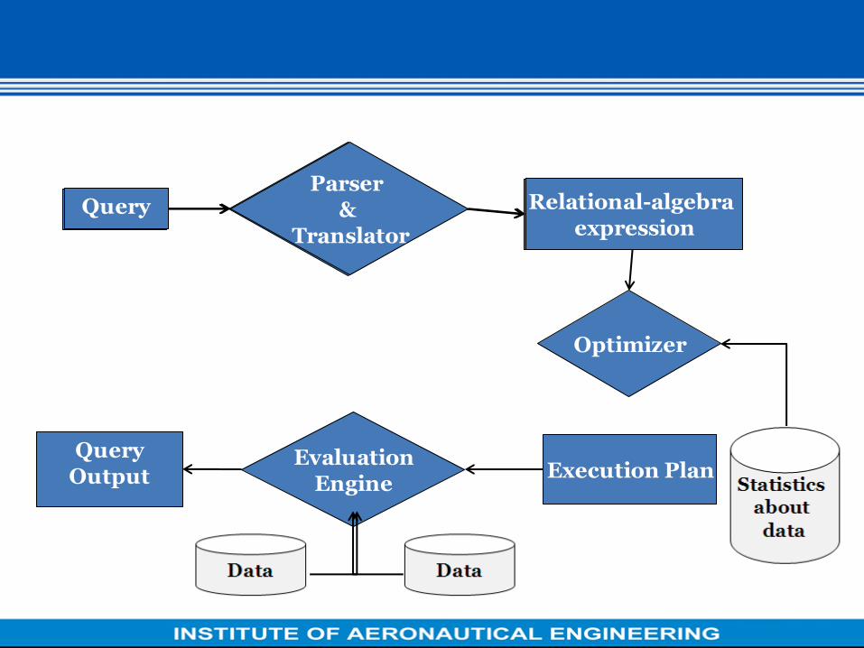
Query
Parser &
Translator
Relational-algebra expression
Optimizer
Execution Plan Evaluation
Engine
Query Output
Query Parser
& Translator
Relational-algebra expression

Basic Steps in Query Processing
• Parsing and translation
– translate the query into its internal form. This is then translated
into relational algebra.
– Parser checks syntax, verifies relations
• Evaluation
– The query-execution engine takes a query-evaluation plan,
executes that plan, and returns the answers to the query.

Basic Steps in Query Processing: Optimization
• A relational algebra expression may have many equivalent
expressions
– E.g., salary75000(salary(instructor)) is equivalent to
salary(salary75000(instructor))
• Each relational algebra operation can be evaluated using one of
several different algorithms
– Correspondingly, a relational-algebra expression can be evaluated in
many ways.
• Annotated expression specifying detailed evaluation strategy is
called an evaluation-plan.
– E.g., can use an index on salary to find instructors with salary < 75000,
– or can perform complete relation scan and discard instructors with
salary 75000

Basic Steps: Optimization (Cont.)
• Query Optimization: Amongst all equivalent evaluation plans choose the one
with lowest cost.
– Cost is estimated using statistical information from the
database catalog
• e.g. number of tuples in each relation, size of tuples, etc.