data mining/machine learning large data sets · data mining/machine learning i large data sets i...
TRANSCRIPT

Data mining/machine learningI large data sets
I high dimensional spacesI potentially little information on structureI computationally intensiveI plots are essential, but complicatedI emphasis on means and variances
STA 302 or 442 (Applied Statistics)
I small data setsI low dimensionI lots of information on the structureI plots are useful, and easy to useI emphasis on likelihood and inference using probability
distributions
: , 1

Data mining/machine learningI large data setsI high dimensional spaces
I potentially little information on structureI computationally intensiveI plots are essential, but complicatedI emphasis on means and variances
STA 302 or 442 (Applied Statistics)
I small data setsI low dimensionI lots of information on the structureI plots are useful, and easy to useI emphasis on likelihood and inference using probability
distributions
: , 2

Data mining/machine learningI large data setsI high dimensional spacesI potentially little information on structure
I computationally intensiveI plots are essential, but complicatedI emphasis on means and variances
STA 302 or 442 (Applied Statistics)
I small data setsI low dimensionI lots of information on the structureI plots are useful, and easy to useI emphasis on likelihood and inference using probability
distributions
: , 3

Data mining/machine learningI large data setsI high dimensional spacesI potentially little information on structureI computationally intensive
I plots are essential, but complicatedI emphasis on means and variances
STA 302 or 442 (Applied Statistics)
I small data setsI low dimensionI lots of information on the structureI plots are useful, and easy to useI emphasis on likelihood and inference using probability
distributions
: , 4

Data mining/machine learningI large data setsI high dimensional spacesI potentially little information on structureI computationally intensiveI plots are essential, but complicated
I emphasis on means and variances
STA 302 or 442 (Applied Statistics)
I small data setsI low dimensionI lots of information on the structureI plots are useful, and easy to useI emphasis on likelihood and inference using probability
distributions
: , 5

Data mining/machine learningI large data setsI high dimensional spacesI potentially little information on structureI computationally intensiveI plots are essential, but complicatedI emphasis on means and variances
STA 302 or 442 (Applied Statistics)
I small data setsI low dimensionI lots of information on the structureI plots are useful, and easy to useI emphasis on likelihood and inference using probability
distributions
: , 6

Data mining/machine learningI large data setsI high dimensional spacesI potentially little information on structureI computationally intensiveI plots are essential, but complicatedI emphasis on means and variances
STA 302 or 442 (Applied Statistics)I small data sets
I low dimensionI lots of information on the structureI plots are useful, and easy to useI emphasis on likelihood and inference using probability
distributions
: , 7

Data mining/machine learningI large data setsI high dimensional spacesI potentially little information on structureI computationally intensiveI plots are essential, but complicatedI emphasis on means and variances
STA 302 or 442 (Applied Statistics)I small data setsI low dimension
I lots of information on the structureI plots are useful, and easy to useI emphasis on likelihood and inference using probability
distributions
: , 8

Data mining/machine learningI large data setsI high dimensional spacesI potentially little information on structureI computationally intensiveI plots are essential, but complicatedI emphasis on means and variances
STA 302 or 442 (Applied Statistics)I small data setsI low dimensionI lots of information on the structure
I plots are useful, and easy to useI emphasis on likelihood and inference using probability
distributions
: , 9

Data mining/machine learningI large data setsI high dimensional spacesI potentially little information on structureI computationally intensiveI plots are essential, but complicatedI emphasis on means and variances
STA 302 or 442 (Applied Statistics)I small data setsI low dimensionI lots of information on the structureI plots are useful, and easy to use
I emphasis on likelihood and inference using probabilitydistributions
: , 10

Data mining/machine learningI large data setsI high dimensional spacesI potentially little information on structureI computationally intensiveI plots are essential, but complicatedI emphasis on means and variances
STA 302 or 442 (Applied Statistics)I small data setsI low dimensionI lots of information on the structureI plots are useful, and easy to useI emphasis on likelihood and inference using probability
distributions
: , 11

Examples (Read Chapter 1, 2.1–2.3)
I email spam 4601 messages, frequencies of 57 commonlyoccurring words
I prostrate cancer 97 patients, 9 covariatesI DNA microarray data 64 samples, 6830 genesI wine data 178 wines, 3 cultivars, 13 covariates
Next week : 3.1-3.3 or 4(3.2.0 should be familiar)
: , 12

Examples (Read Chapter 1, 2.1–2.3)
I email spam 4601 messages, frequencies of 57 commonlyoccurring words
I prostrate cancer 97 patients, 9 covariates
I DNA microarray data 64 samples, 6830 genesI wine data 178 wines, 3 cultivars, 13 covariates
Next week : 3.1-3.3 or 4(3.2.0 should be familiar)
: , 13

Examples (Read Chapter 1, 2.1–2.3)
I email spam 4601 messages, frequencies of 57 commonlyoccurring words
I prostrate cancer 97 patients, 9 covariatesI DNA microarray data 64 samples, 6830 genes
I wine data 178 wines, 3 cultivars, 13 covariates
Next week : 3.1-3.3 or 4(3.2.0 should be familiar)
: , 14

Examples (Read Chapter 1, 2.1–2.3)
I email spam 4601 messages, frequencies of 57 commonlyoccurring words
I prostrate cancer 97 patients, 9 covariatesI DNA microarray data 64 samples, 6830 genesI wine data 178 wines, 3 cultivars, 13 covariates
Next week : 3.1-3.3 or 4(3.2.0 should be familiar)
: , 15

Elements of Statistical Learning c©Hastie, Tibshirani & Friedman 2001 Chapter 1
lpsa
-1 1 3
oooooo ooo ooo ooooo oo o o oo oo ooo o ooo ooo ooo ooo oo ooo oo ooo oo o ooooooo o oooo ooo o ooo o ooooooo oooo ooo oo ooo
ooo o
o oo ooooooooooo oo ooo ooooooo oooo o oooo ooo ooo ooooo oooo ooo oo oo o oo ooo ooooooooo oo oo ooooo o oooooo oo ooo
oooo40 60 80
o o oooo ooo oooo oo o ooo oooo o oooooooo oo oo oo oo o ooo oo ooo oooo oo ooo oo oo oooo o oooo ooo oo o ooooo ooo oooo ooo oo o oo
oooooo o oooo ooooo ooo oo oo o ooo ooo ooooo ooo oooo oo oo ooo oo oooo oo oo o ooo oo o o oo oo oo oo o oooo ooo o oo ooo oo oooo oo
0.0 0.4 0.8
oooooooooooooooooooooooooooooooooooooo oooooooo ooooooooooooooo oo ooooooo oo oooooo oooo ooo oo oooo oo
oooo
oooooooooooo oo oo o oooo oo ooo oo o ooooo oo oo oooo o ooo ooo ooo o ooo ooooo oo oo o ooo o oo o o o ooo ooo oo oo oo o oooo o ooo o
6.0 7.5 9.0
oo oooooooooo oooo ooooo oo ooo ooooooooo o oooo ooo ooo oooo oo oooooo ooo o ooo oooo oooo oooooooooo oooo oooo oo
oooo
01
23
45
oo oooooooooo oooo ooooo oo ooo oo oooooooooo oo oooo oo oooo oo oooooo o oo o ooo o oooo ooo oo ooo ooo oo oo oo o o oo o ooo oo
-10
12
34
oooo
o
o
oo
ooo
o
oooo
o
o
oooo
o
o
oooo
o
o
oo
o
oo
ooo
o
oooo
oooo
ooooo
o
oo
oooooo
ooooooo
o
ooooo
oo
oooo
oooo
o
o
oo
o
o
ooo
oooo
lcavol
o oo
o
o
o
oo
ooo
o
oo oo
o
o
oo
oo
o
o
oo
oo
o
o
o o
o
oo
ooo
o
oooo
oooo
ooo o
o
o
oo
ooo oo
o
oo
ooooo
o
oo
o oo
oo
oooo
oo oo
o
o
oo
o
o
oooo
ooo
o oo
o
o
o
oo
ooo
o
o oo o
o
o
oo
oo
o
o
oo
oo
o
o
oo
o
o o
o oo
o
o oo
o
o ooo
oo
ooo
o
oo
ooo o
oo
oo
ooo
o o
o
oo
ooo
oo
oooo
oo oo
o
o
oo
o
o
oo o
oo o
o
oooo
o
o
o o
ooo
o
oooo
o
o
oo
oo
o
o
oo
oo
o
o
oo
o
oo
ooo
o
ooo
o
o ooo
oo
ooo
o
oo
ooooo
o
oo
ooo
o o
o
oo
ooo
o o
oooo
ooo o
o
o
oo
o
o
ooo
oo o
o
oooo
o
o
oo
ooo
o
oooo
o
o
oooo
o
o
oooo
o
o
oo
o
oo
ooo
o
oooo
oooo
ooooo
o
oo
oooooo
oo
ooooo
o
oo
o oo
oo
oo oo
oo oo
o
o
o o
o
o
ooooooo
oooo
o
o
oo
ooo
o
oo oo
o
o
ooo
o
o
o
oo
oo
o
o
oo
o
o o
o oo
o
ooo
o
oooo
oo
ooo
o
oo
o ooooo
oo
ooo
oo
o
oo
o oo
o o
oo oo
ooo o
o
o
o o
o
o
oo o
ooo
o
ooo
o
o
o
oo
ooo
o
oooo
o
o
ooo
o
o
o
oo
oo
o
o
oo
o
oo
o oo
o
o oo
o
oooo
ooo oo
o
oo
ooo o
oo
oo
ooooo
o
oooo
o
oo
oooo
ooo o
o
o
o o
o
o
ooooooo
ooo
o
o
o
oo
ooo
o
oooo
o
o
ooo
o
o
o
oo
oo
o
o
oo
o
oo
ooo
o
o oo
o
o ooo
ooo oo
o
oo
ooo o
oo
oo
ooo
oo
o
oo
ooo
o o
oo oo
ooo o
o
o
o o
o
o
oo o
oo o
o
oooooooooo
ooooooooooooooooooooo
o
ooo
oo
o
o
ooooooooooooooooo
o
oooo
ooooooooo
oooooo
oooooooooooo
o
oooooo
oo
oo
oo oo ooo o
oooo
oo
o oo
oo oo ooo
ooo o
o
o
ooo
oo
o
o
oooo ooo
oooo
o oo
oo
o
o
oo
oo
o oooo oo
oo
ooo
ooo
oooo
ooooo oo
o
o
oo
oo ooo o lweight
oo
oooo ooo o
ooo o
oo
ooo
oooo o o
ooooo
o
o
oo o
oo
o
o
o oooo
oooo
o ooo
oo
oo
o
oo
oo
o oooo o ooo
o oo
ooo
o ooo
oo
ooo ooo
o
oo
o ooo
oo
oooooo o oooo ooooo
ooo
oo oo o o
oo o
ooo
o
ooo
oo
o
o
ooo oo
oooo
o oo o
oo
oo
o
oo
oo
oooo o o o
oo
o oo
oo
o
oooo
oo
o o oo oo
o
oo
oooo
oo
ooooooooooooooooooooooooooooooo
o
ooo
oo
o
o
ooooooo
oooooooooo
o
oooo
oooooo
ooo
oooooo
oooo
oo
ooo ooo
o
oo
oooooo
oooooooooooo
ooo
oo o
ooo oo ooo
ooo o
o
o
oo o
oo
o
o
ooo o o
oooo
o ooo
oo
oo
o
oooo
oooo o oo
oo
ooo
oo
o
oooo
oo
o oo ooo
o
ooo o o
oo o
oo
oooooooooo
ooo
ooo
ooo oo ooo
oooo
o
o
ooo
oo
o
o
o ooo ooo
oooo
oooooo
o
ooo
o
o ooo ooo
oo
ooo
ooo
ooooooo ooooo
o
oo
oooooo
34
56
oo
oooooooooo
ooo
ooo
ooo oo ooo
oooo
o
o
ooo
oo
o
o
o oooo
oooo
oooo
oo
oo
o
oo
oo
o ooo o oo
oo
ooo
oo
o
oooo
oo
o oo ooo
o
oo
o ooo
oo
4050
6070
80
o
o
o
oo
o
oo
o
ooooo
o
ooo
o
o
ooooooooooooo
o
oo
o
oo
oo
ooooo
o
o
o
ooooo
oo
oo
o
o
o
o
oooooooo
o
o
o
o
oooo
ooo
o
o
oooooo
o
ooo
oo
oo
o
o
o
oo
o
oo
o
ooo oo
o
oo
o
o
o
o ooo
o ooo o oooo
o
o o
o
oo
oo
oo o
oo
o
o
o
oooo
o
oo
oo
o
o
o
o
ooooooo o
o
o
o
o
ooo
o
ooo
o
o
oo
oo
o o
o
ooo
oo
o o
o
o
o
oo
o
oo
o
ooooo
o
ooo
o
o
oooooo oooo o o
o
o
o o
o
oo
oo
ooo
oo
o
o
o
o oooo
oo
o o
o
o
o
o
oooooooo
o
o
o
o
oooo
ooo
o
o
oo
oo
o o
o
ooo
oo
oo
ageo
o
o
oo
o
oo
o
oo ooo
o
oo
o
o
o
o ooo
ooo ooo ooo
o
o o
o
oo
oo
oooo
o
o
o
o
oooo
o
oo
o o
o
o
o
o
ooo o
ooo o
o
o
o
o
o ooo
oo o
o
o
oo
oo
oo
o
oo
o
oo
oo
o
o
o
oo
o
oo
o
ooooo
o
ooo
o
o
ooooooooooooo
o
oo
o
oo
oo
ooooo
o
o
o
ooooo
oo
oo
o
o
o
o
oooo
oooo
o
o
o
o
oooo
ooo
o
o
oo
oo
oo
o
ooo
oo
oo
o
o
o
oo
o
oo
o
ooo oo
o
oo
o
o
o
o ooo
oo oo o oooo
o
oo
o
oo
oo
oo oo
o
o
o
o
ooo o
o
oo
oo
o
o
o
o
ooo o
ooo o
o
o
o
o
o oo
o
ooo
o
o
oo
oo
o o
o
oo
o
oo
o o
o
o
o
oo
o
oo
o
ooo oo
o
oo
o
o
o
o ooo
oo ooooooo
o
o o
o
oo
oo
oo o
oo
o
o
o
o oo o
o
oo
oo
o
o
o
o
ooo oooo o
o
o
o
o
oooo
ooo
o
o
ooo
ooo
o
ooo
oo
oo
o
o
o
oo
o
oo
o
ooo oo
o
oo
o
o
o
o ooo
oo oo ooooo
o
oo
o
oo
oo
ooo
oo
o
o
o
o oo o
o
oo
oo
o
o
o
o
ooo o
oooo
o
o
o
o
o oo
o
ooo
o
o
oo
oo
o o
o
oo
o
oo
oo
oooooo
o
o
ooo
o
oooo
o
oo
o
o
o
o
o
o
o
o
o
o
o
ooo
oo
o
o
o
oo
oo
o
o
o
o
oo
o
o
o
ooo
o
o
o
o
o
o
oo
o
o
o
ooo
o
o
o
o
o
o
o
o
oo
oo
oo
o
oo
o
o
oo
o
o
o
ooo
o
o
oooo oo
o
o
o oo
o
oooo
o
oo
o
o
o
o
o
o
o
o
o
o
o
ooo
oo
o
o
o
oo
o o
o
o
o
o
oo
o
o
o
oo o
o
o
o
o
o
o
oo
o
o
o
ooo
o
o
o
o
o
o
o
o
oo
oo
o o
o
oo
o
o
o o
o
o
o
o oo
o
o
o oo ooo
o
o
ooo
o
oo oo
o
oo
o
o
o
o
o
o
o
o
o
o
o
o oo
oo
o
o
o
oo
o o
o
o
o
o
oo
o
o
o
oo o
o
o
o
o
o
o
oo
o
o
o
ooo
o
o
o
o
o
o
o
o
oo
oo
o o
o
oo
o
o
o o
o
o
o
ooo
o
o
o o oooo
o
o
o oo
o
o oo o
o
oo
o
o
o
o
o
o
o
o
o
o
o
ooo
o o
o
o
o
oo
o o
o
o
o
o
oo
o
o
o
oo o
o
o
o
o
o
o
oo
o
o
o
oo
o
o
o
o
o
o
o
o
o
o o
oo
oo
o
oo
o
o
oo
o
o
o
oo o
o
o lbph
oooooo
o
o
ooo
o
oooo
o
oo
o
o
o
o
o
o
o
o
o
o
o
ooo
oo
o
o
o
oo
oo
o
o
o
o
oo
o
o
o
ooo
o
o
o
o
o
o
oo
o
o
o
ooo
o
o
o
o
o
o
o
o
oo
oo
oo
o
oo
o
o
oo
o
o
o
ooo
o
o
oooooo
o
o
ooo
o
oo oo
o
oo
o
o
o
o
o
o
o
o
o
o
o
ooo
o o
o
o
o
oo
oo
o
o
o
o
oo
o
o
o
oo o
o
o
o
o
o
o
oo
o
o
o
oo
o
o
o
o
o
o
o
o
o
oo
oo
o o
o
oo
o
o
o o
o
o
o
o oo
o
o
oo oooo
o
o
ooo
o
oooo
o
oo
o
o
o
o
o
o
o
o
o
o
o
ooo
oo
o
o
o
oo
oo
o
o
o
o
oo
o
o
o
ooo
o
o
o
o
o
o
oo
o
o
o
ooo
o
o
o
o
o
o
o
o
oo
oo
oo
o
oo
o
o
oo
o
o
o
ooo
o
o
-10
12
oo oooo
o
o
ooo
o
oooo
o
oo
o
o
o
o
o
o
o
o
o
o
o
ooo
oo
o
o
o
oo
oo
o
o
o
o
oo
o
o
o
ooo
o
o
o
o
o
o
oo
o
o
o
oo
o
o
o
o
o
o
o
o
o
oo
oo
o o
o
oo
o
o
o o
o
o
o
ooo
o
o
0.0
0.4
0.8
oooooooooooooooooooooooooooooooooooooo
o
ooooooo
o
oooooooooooooo
o
o
o
oooooo
o
o
oooo
oo
o
ooo
o
oo
o
o
ooo
o
oooooo
oooo oo ooo ooo ooooo oo o o oo oo ooo o ooo ooo ooo
o
oo oo ooo
o
o ooo oo o ooooooo
o
o
o
oo ooo o
o
o
o o oo
oo
o
oo o
o
oo
o
o
o oo
o
oo ooo o
o oo ooooooooooo oo ooo ooooooo oooo o oooo ooo
o
oo ooooo
o
ooo ooo oo oo o oo o
o
o
o
oooooo
o
o
oo oo
oo
o
oo o
o
oo
o
o
o oo
o
oooooo
o o oooo ooo oooo oo o ooo oooo o oooooooo oo oo oo
o
o o ooo oo
o
oo oooo oo ooo oo o
o
o
o
oo o ooo
o
o
oo oo
o o
o
ooo
o
oo
o
o
oo o
o
o oo o oo
oooooo o oooo ooooo ooo oo oo o ooo ooo ooooo ooo
o
ooo oo oo
o
oo oo oooo oo oo o o
o
o
o
o o o oo o
o
o
o oo o
oo
o
o oo
o
o o
o
o
oo o
o
oooo oo
svi
oooooooooooo oo oo o oooo oo ooo oo o ooooo oo oo
o
ooo o ooo
o
oo ooo o ooo ooooo
o
o
o
o o ooo o
o
o
o o o o
oo
o
oo o
o
oo
o
o
o oo
o
o o ooo o
oo oooooooooo oooo ooooo oo ooo ooooooooo o oo
o
o ooo ooo
o
ooo oo oooooo ooo
o
o
o
o oooo o
o
o
o ooo
oo
o
ooo
o
oo
o
o
ooo
o
oooooo
oo oooooooooo oooo ooooo oo ooo oo oooooooooo
o
o oooo oo
o
ooo oo oooooo o oo
o
o
o
o o oooo
o
o
o oo o
oo
o
oo o
o
oo
o
o
o o o
o
o ooo oo
oooooooooooooo
o
oo
o
ooo
o
o
o
oooo
o
o
oooooo
o
o
o
o
oo
o
o
o
o
o
o
oooo
o
o
oo
o
oooo
ooo
o
o
o
o
oo
o
o
o
ooo
o
o
o
oo
o
o
o
o
o
o
o
o
o
oo
ooo
o
o
oooo oo ooo ooooo
o
oo
o
o o o
o
o
o
o oo
o
o
o
oo ooo
o
o
o
o
o
o o
o
o
o
o
o
o
ooo o
o
o
oo
o
oooo
o oo
o
o
o
o
oo
o
o
o
ooo
o
o
o
oo
o
o
o
o
o
o
o
o
o
oo
ooo
o
o
o oo ooooooooooo
o
oo
o
o oo
o
o
o
oooo
o
o
oooo
oo
o
o
o
o
o o
o
o
o
o
o
o
oo
oo
o
o
o o
o
o oo o
ooo
o
o
o
o
oo
o
o
o
oo
o
o
o
o
oo
o
o
o
o
o
o
o
o
o
oo
ooo
o
o
o o oooo ooo oooo
o
o
oo
o
o oo
o
o
o
oooo
o
o
oo oo
oo
o
o
o
o
o o
o
o
o
o
o
o
oo
oo
o
o
o o
o
o oo o
o oo
o
o
o
o
oo
o
o
o
ooo
o
o
o
oo
o
o
o
o
o
o
o
o
o
oo
oo o
o
o
oooooo o oooo ooo
o
oo
o
o oo
o
o
o
ooo
o
o
o
oooo
oo
o
o
o
o
oo
o
o
o
o
o
o
oo
o o
o
o
o o
o
oo o o
ooo
o
o
o
o
oo
o
o
o
oo
o
o
o
o
o o
o
o
o
o
o
o
o
o
o
o o
ooo
o
o
oooooooooooooo
o
oo
o
ooo
o
o
o
oooo
o
o
oooooo
o
o
o
o
oo
o
o
o
o
o
o
oooo
o
o
oo
o
oooo
ooo
o
o
o
o
oo
o
o
o
ooo
o
o
o
oo
o
o
o
o
o
o
o
o
o
o o
ooo
o
o
lcp
oo oooooooooooo
o
oo
o
ooo
o
o
o
oooo
o
o
ooooo
o
o
o
o
o
oo
o
o
o
o
o
o
oo
oo
o
o
oo
o
o ooo
o oo
o
o
o
o
oo
o
o
o
ooo
o
o
o
oo
o
o
o
o
o
o
o
o
o
o o
ooo
o
o
-10
12
3
oo ooooooooooo
o
o
oo
o
ooo
o
o
o
ooo
o
o
o
oooooo
o
o
o
o
oo
o
o
o
o
o
o
oo
oo
o
o
oo
o
o o oo
o oo
o
o
o
o
oo
o
o
o
oo
o
o
o
o
oo
o
o
o
o
o
o
o
o
o
o o
ooo
o
o
6.0
7.0
8.0
9.0
oo
o
ooooooooo
ooo
o
o
oooo
o
o
o
oo
ooo
oooooo
o
o
ooo
o
o
o
ooo
o
o
oo
o
o
ooooo
o
oo
o
o
o
o
o
ooo
o
oooo
o
ooooooooo
o
oo
o
ooo
o
oooooo
oo
o
o oo ooo ooo
ooo
o
o
oo o o
o
o
o
o o
oo o
ooo ooo
o
o
o oo
o
o
o
ooo
o
o
oo
o
o
o o ooo
o
oo
o
o
o
o
o
o oo
o
o ooo
o
ooooooo oo
o
o o
o
o oo
o
oo ooo o
o o
o
ooooooooo
oo o
o
o
oo oo
o
o
o
oo
ooo
o o oooo
o
o
o oo
o
o
o
ooo
o
o
oo
o
o
o oo oo
o
oo
o
o
o
o
o
ooo
o
ooo o
o
oo ooooo o o
o
oo
o
o oo
o
oooooo
o o
o
ooo ooo ooo
o oo
o
o
oo oo
o
o
o
oo
ooo
ooo oo o
o
o
o oo
o
o
o
o oo
o
o
o o
o
o
o oo oo
o
oo
o
o
o
o
o
o o o
o
oo oo
o
oo o ooooo o
o
o o
o
oo o
o
o oo o oo
oo
o
ooo o oooo o
ooo
o
o
oo oo
o
o
o
oo
o oo
o ooooo
o
o
o oo
o
o
o
o oo
o
o
o o
o
o
ooo oo
o
o o
o
o
o
o
o
o o o
o
oo oo
o
o o oooo ooo
o
oo
o
oo o
o
oooo oo
oo
o
ooooooooo
ooo
o
o
oooo
o
o
o
oo
ooo
oooooo
o
o
o oo
o
o
o
ooo
o
o
oo
o
o
ooooo
o
oo
o
o
o
o
o
ooo
o
o oo o
o
oooo oooo o
o
o o
o
ooo
o
oooooo
oo
o
ooooooooo
oo o
o
o
oooo
o
o
o
oo
oo o
ooooo o
o
o
o oo
o
o
o
ooo
o
o
o o
o
o
o ooo o
o
oo
o
o
o
o
o
o oo
o
o oo o
o
o ooo ooo oo
o
o o
o
o oo
o
o o ooo ogleason
oo
o
ooooooooo
ooo
o
o
oooo
o
o
o
oo
oo o
oooooo
o
o
o oo
o
o
o
o oo
o
o
oo
o
o
ooooo
o
o o
o
o
o
o
o
o oo
o
o ooo
o
o ooo ooo oo
o
o o
o
o o o
o
o ooo oo
0 2 4oooooooooooo
o
ooo
o
oooooo
o
oo
o
o
o
oooooooooo
o
o
ooooo
o
o
oo
o
o
o
o
oooooo
o
o
o
o
oo
o
ooo
o
oo
o
o
oo
o
oooo
o
o
o
o
o
o
oo
oo
oo
o
o
oooo
o oo ooo ooo
o
ooo
o
oo o oo
o
o
o o
o
o
o
ooo ooo ooo
o
o
o
oo o
oo
o
o
oo
o
o
o
o
oo
ooo
o
o
o
o
o
oo
o
oo o
o
oo
o
o
oo
o
oo
oo
o
o
o
o
o
o
oo
oo
oo
o
o
o
3 4 5 6o oo
ooooooooo
o
o oo
o
oo oooo
o
oo
o
o
o
o o oooo ooo
o
o
o
ooo
oo
o
o
oo
o
o
o
o
oo
o oo
o
o
o
o
o
oo
o
ooo
o
o o
o
o
oo
o
oo
oo
o
o
o
o
o
o
oo
oo
oo
o
o
oo o
oooo ooo ooo
o
oo o
o
oo oooo
o
oo
o
o
o
ooo oo oooo
o
o
o
ooo
oo
o
o
o o
o
o
o
o
oo
ooo
o
o
o
o
o
oo
o
ooo
o
oo
o
o
oo
o
ooo
o
o
o
o
o
o
o
oo
oo
oo
o
o
o
-1 0 1 2oooooo o oooo o
o
ooo
o
oo ooo
o
o
oo
o
o
o
o ooooo ooo
o
o
o
ooooo
o
o
o o
o
o
o
o
oo
o oo
o
o
o
o
o
oo
o
oo o
o
oo
o
o
oo
o
oo
oo
o
o
o
o
o
o
oo
oo
oo
o
o
ooooooooooooo
o
ooo
o
oooooo
o
oo
o
o
o
ooooooooo
o
o
o
ooooo
o
o
oo
o
o
o
o
oooooo
o
o
o
o
oo
o
ooo
o
o o
o
o
oo
o
oooo
o
o
o
o
o
o
oo
oo
oo
o
o
o
-1 1 2 3oooooooooooo
o
o oo
o
ooooo
o
o
oo
o
o
o
ooooo ooooo
o
o
oo ooo
o
o
o o
o
o
o
o
oo
oooo
o
o
o
o
oo
o
oo o
o
o o
o
o
oo
o
ooo
o
o
o
o
o
o
o
oo
oo
oo
o
o
ooo
oooooooooo
o
ooo
o
ooooo
o
o
oo
o
o
o
oooooo ooo
o
o
o
oo o
oo
o
o
oo
o
o
o
o
oooooo
o
o
o
o
oo
o
oo o
o
oo
o
o
oo
o
oooo
o
o
o
o
o
o
oo
oo
oo
o
o
o
0 40 80
020
6010
0
pgg45
Figure 1.1: Scatterplot matrix of the prostate cancer
data. The first row shows the response against each of
the predictors in turn. Two of the predictors, svi and
gleason, are categorical.
: , 16

Some of the wine data:1,14.23,1.71,2.43,15.6,127,2.8,3.06,.28,2.29,5.64,1.04,3.92,10651,13.2,1.78,2.14,11.2,100,2.65,2.76,.26,1.28,4.38,1.05,3.4,10501,13.16,2.36,2.67,18.6,101,2.8,3.24,.3,2.81,5.68,1.03,3.17,11851,14.37,1.95,2.5,16.8,113,3.85,3.49,.24,2.18,7.8,.86,3.45,14801,13.24,2.59,2.87,21,118,2.8,2.69,.39,1.82,4.32,1.04,2.93,7351,14.2,1.76,2.45,15.2,112,3.27,3.39,.34,1.97,6.75,1.05,2.85,14501,14.39,1.87,2.45,14.6,96,2.5,2.52,.3,1.98,5.25,1.02,3.58,12901,14.06,2.15,2.61,17.6,121,2.6,2.51,.31,1.25,5.05,1.06,3.58,12951,14.83,1.64,2.17,14,97,2.8,2.98,.29,1.98,5.2,1.08,2.85,10451,13.86,1.35,2.27,16,98,2.98,3.15,.22,1.85,7.22,1.01,3.55,10451,14.1,2.16,2.3,18,105,2.95,3.32,.22,2.38,5.75,1.25,3.17,15101,14.12,1.48,2.32,16.8,95,2.2,2.43,.26,1.57,5,1.17,2.82,12801,13.75,1.73,2.41,16,89,2.6,2.76,.29,1.81,5.6,1.15,2.9,13201,14.75,1.73,2.39,11.4,91,3.1,3.69,.43,2.81,5.4,1.25,2.73,11501,14.38,1.87,2.38,12,102,3.3,3.64,.29,2.96,7.5,1.2,3,15471,13.63,1.81,2.7,17.2,112,2.85,2.91,.3,1.46,7.3,1.28,2.88,13101,14.3,1.92,2.72,20,120,2.8,3.14,.33,1.97,6.2,1.07,2.65,12801,13.83,1.57,2.62,20,115,2.95,3.4,.4,1.72,6.6,1.13,2.57,11301,14.19,1.59,2.48,16.5,108,3.3,3.93,.32,1.86,8.7,1.23,2.82,16801,13.64,3.1,2.56,15.2,116,2.7,3.03,.17,1.66,5.1,.96,3.36,8451,14.06,1.63,2.28,16,126,3,3.17,.24,2.1,5.65,1.09,3.71,7801,12.93,3.8,2.65,18.6,102,2.41,2.41,.25,1.98,4.5,1.03,3.52,7701,13.71,1.86,2.36,16.6,101,2.61,2.88,.27,1.69,3.8,1.11,4,10351,12.85,1.6,2.52,17.8,95,2.48,2.37,.26,1.46,3.93,1.09,3.63,10151,13.5,1.81,2.61,20,96,2.53,2.61,.28,1.66,3.52,1.12,3.82,845
1,13.05,2.05,3.22,25,124,2.63,2.68,.47,1.92,3.58,1.13,3.2,830
: , 17

1 5 10 30 1.0 0.2 2 12 1.5
1114
14
ash
1.53.0
1025
80160
1.03.5
14
0.2
0.53.5
28
hue
0.61.6
1.54.0
11 1.5 80 1 5 0.5 0.6 400
400
: , 18

alcohol
1 2 3 4 5 6 10 15 20 25 30
1112
1314
12
34
56
malic acid
ash
1.52.0
2.53.0
11 12 13 14
1015
2025
30
1.5 2.5
alcalinity of ash
: , 19

Some basic definitionsinput X (features), output Y (response)
data (xi , yi), i = 1, . . . Nuse data to assign a rule (function) taking X → Ygoal is to predict a new value of Y , given X : Y (X )
regression if Y is continuousclassification if Y is discrete
: , 20

Some basic definitionsinput X (features), output Y (response)data (xi , yi), i = 1, . . . N
use data to assign a rule (function) taking X → Ygoal is to predict a new value of Y , given X : Y (X )
regression if Y is continuousclassification if Y is discrete
: , 21

Some basic definitionsinput X (features), output Y (response)data (xi , yi), i = 1, . . . Nuse data to assign a rule (function) taking X → Y
goal is to predict a new value of Y , given X : Y (X )
regression if Y is continuousclassification if Y is discrete
: , 22

Some basic definitionsinput X (features), output Y (response)data (xi , yi), i = 1, . . . Nuse data to assign a rule (function) taking X → Ygoal is to predict a new value of Y , given X : Y (X )
regression if Y is continuousclassification if Y is discrete
: , 23

Some basic definitionsinput X (features), output Y (response)data (xi , yi), i = 1, . . . Nuse data to assign a rule (function) taking X → Ygoal is to predict a new value of Y , given X : Y (X )
regression if Y is continuousclassification if Y is discrete
: , 24

How to know if the rule works?compare yi to yi on data training error
compare Y to Y on new data test error
In ordinary linear regression, the least squares estimatesminimize
Σ(yi − β0 − β1xi)2
and the minimized value is the sum of the squared residuals
Σ(yi − yi)2 = Σ(yi − β0 − β1xi)
2
: , 25

How to know if the rule works?compare yi to yi on data training errorcompare Y to Y on new data test error
In ordinary linear regression, the least squares estimatesminimize
Σ(yi − β0 − β1xi)2
and the minimized value is the sum of the squared residuals
Σ(yi − yi)2 = Σ(yi − β0 − β1xi)
2
: , 26

How to know if the rule works?compare yi to yi on data training errorcompare Y to Y on new data test error
In ordinary linear regression, the least squares estimatesminimize
Σ(yi − β0 − β1xi)2
and the minimized value is the sum of the squared residuals
Σ(yi − yi)2 = Σ(yi − β0 − β1xi)
2
: , 27

A complex regression model: NMMAPS (NationalMorbidity, Mortality and Air Pollution Study)
I 90 largest cities in US by population (US Census)
I daily mortality counts from NCHS (National Center forHealth Statistics) 1987–1994
I hourly temperature and dewpoint data from NationalClimatic data Center
I data on pollutants PM10, O3, CO, SO2, NO2 from EPAI output: Yt mortality rate on day tI inputs: Xt pollution on day t − 1, plus various confounders:
age and size of population, weather, day of the week, timeI a model was fit for each city, and aggregated over citiesI Conclusion 0.41% increase in mortality for a 10 µg
increase in PM10
: , 28

A complex regression model: NMMAPS (NationalMorbidity, Mortality and Air Pollution Study)
I 90 largest cities in US by population (US Census)I daily mortality counts from NCHS (National Center for
Health Statistics) 1987–1994
I hourly temperature and dewpoint data from NationalClimatic data Center
I data on pollutants PM10, O3, CO, SO2, NO2 from EPAI output: Yt mortality rate on day tI inputs: Xt pollution on day t − 1, plus various confounders:
age and size of population, weather, day of the week, timeI a model was fit for each city, and aggregated over citiesI Conclusion 0.41% increase in mortality for a 10 µg
increase in PM10
: , 29

A complex regression model: NMMAPS (NationalMorbidity, Mortality and Air Pollution Study)
I 90 largest cities in US by population (US Census)I daily mortality counts from NCHS (National Center for
Health Statistics) 1987–1994I hourly temperature and dewpoint data from National
Climatic data Center
I data on pollutants PM10, O3, CO, SO2, NO2 from EPAI output: Yt mortality rate on day tI inputs: Xt pollution on day t − 1, plus various confounders:
age and size of population, weather, day of the week, timeI a model was fit for each city, and aggregated over citiesI Conclusion 0.41% increase in mortality for a 10 µg
increase in PM10
: , 30

A complex regression model: NMMAPS (NationalMorbidity, Mortality and Air Pollution Study)
I 90 largest cities in US by population (US Census)I daily mortality counts from NCHS (National Center for
Health Statistics) 1987–1994I hourly temperature and dewpoint data from National
Climatic data CenterI data on pollutants PM10, O3, CO, SO2, NO2 from EPA
I output: Yt mortality rate on day tI inputs: Xt pollution on day t − 1, plus various confounders:
age and size of population, weather, day of the week, timeI a model was fit for each city, and aggregated over citiesI Conclusion 0.41% increase in mortality for a 10 µg
increase in PM10
: , 31

A complex regression model: NMMAPS (NationalMorbidity, Mortality and Air Pollution Study)
I 90 largest cities in US by population (US Census)I daily mortality counts from NCHS (National Center for
Health Statistics) 1987–1994I hourly temperature and dewpoint data from National
Climatic data CenterI data on pollutants PM10, O3, CO, SO2, NO2 from EPAI output: Yt mortality rate on day t
I inputs: Xt pollution on day t − 1, plus various confounders:age and size of population, weather, day of the week, time
I a model was fit for each city, and aggregated over citiesI Conclusion 0.41% increase in mortality for a 10 µg
increase in PM10
: , 32

A complex regression model: NMMAPS (NationalMorbidity, Mortality and Air Pollution Study)
I 90 largest cities in US by population (US Census)I daily mortality counts from NCHS (National Center for
Health Statistics) 1987–1994I hourly temperature and dewpoint data from National
Climatic data CenterI data on pollutants PM10, O3, CO, SO2, NO2 from EPAI output: Yt mortality rate on day tI inputs: Xt pollution on day t − 1, plus various confounders:
age and size of population, weather, day of the week, time
I a model was fit for each city, and aggregated over citiesI Conclusion 0.41% increase in mortality for a 10 µg
increase in PM10
: , 33

A complex regression model: NMMAPS (NationalMorbidity, Mortality and Air Pollution Study)
I 90 largest cities in US by population (US Census)I daily mortality counts from NCHS (National Center for
Health Statistics) 1987–1994I hourly temperature and dewpoint data from National
Climatic data CenterI data on pollutants PM10, O3, CO, SO2, NO2 from EPAI output: Yt mortality rate on day tI inputs: Xt pollution on day t − 1, plus various confounders:
age and size of population, weather, day of the week, timeI a model was fit for each city, and aggregated over cities
I Conclusion 0.41% increase in mortality for a 10 µgincrease in PM10
: , 34

A complex regression model: NMMAPS (NationalMorbidity, Mortality and Air Pollution Study)
I 90 largest cities in US by population (US Census)I daily mortality counts from NCHS (National Center for
Health Statistics) 1987–1994I hourly temperature and dewpoint data from National
Climatic data CenterI data on pollutants PM10, O3, CO, SO2, NO2 from EPAI output: Yt mortality rate on day tI inputs: Xt pollution on day t − 1, plus various confounders:
age and size of population, weather, day of the week, timeI a model was fit for each city, and aggregated over citiesI Conclusion 0.41% increase in mortality for a 10 µg
increase in PM10
: , 35

: , 36

: , 37

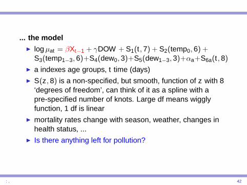
... the modelI log µat = βXt−1 + γDOW + S1(t , 7) + S2(temp0, 6) +
S3(temp1−3, 6)+S4(dew0, 3)+S5(dew1−3, 3)+αa+S6a(t , 8)
I a indexes age groups, t time (days)I S(z, 8) is a non-specified, but smooth, function of z with 8
‘degrees of freedom’, can think of it as a spline with apre-specified number of knots. Large df means wigglyfunction, 1 df is linear
I mortality rates change with season, weather, changes inhealth status, ...
I Is there anything left for pollution?
: , 38

... the modelI log µat = βXt−1 + γDOW + S1(t , 7) + S2(temp0, 6) +
S3(temp1−3, 6)+S4(dew0, 3)+S5(dew1−3, 3)+αa+S6a(t , 8)
I a indexes age groups, t time (days)
I S(z, 8) is a non-specified, but smooth, function of z with 8‘degrees of freedom’, can think of it as a spline with apre-specified number of knots. Large df means wigglyfunction, 1 df is linear
I mortality rates change with season, weather, changes inhealth status, ...
I Is there anything left for pollution?
: , 39

... the modelI log µat = βXt−1 + γDOW + S1(t , 7) + S2(temp0, 6) +
S3(temp1−3, 6)+S4(dew0, 3)+S5(dew1−3, 3)+αa+S6a(t , 8)
I a indexes age groups, t time (days)I S(z, 8) is a non-specified, but smooth, function of z with 8
‘degrees of freedom’, can think of it as a spline with apre-specified number of knots. Large df means wigglyfunction, 1 df is linear
I mortality rates change with season, weather, changes inhealth status, ...
I Is there anything left for pollution?
: , 40

... the modelI log µat = βXt−1 + γDOW + S1(t , 7) + S2(temp0, 6) +
S3(temp1−3, 6)+S4(dew0, 3)+S5(dew1−3, 3)+αa+S6a(t , 8)
I a indexes age groups, t time (days)I S(z, 8) is a non-specified, but smooth, function of z with 8
‘degrees of freedom’, can think of it as a spline with apre-specified number of knots. Large df means wigglyfunction, 1 df is linear
I mortality rates change with season, weather, changes inhealth status, ...
I Is there anything left for pollution?
: , 41
... the modelI log µat = βXt−1 + γDOW + S1(t , 7) + S2(temp0, 6) +
S3(temp1−3, 6)+S4(dew0, 3)+S5(dew1−3, 3)+αa+S6a(t , 8)
I a indexes age groups, t time (days)I S(z, 8) is a non-specified, but smooth, function of z with 8
‘degrees of freedom’, can think of it as a spline with apre-specified number of knots. Large df means wigglyfunction, 1 df is linear
I mortality rates change with season, weather, changes inhealth status, ...
I Is there anything left for pollution?
: , 42

I “the new analysis is highly likely to delay the final review ofnew regulations on small-particle pollution”
I “industry officials said the new findings called into questionthe validity of some research underlying the new federalstandards”
I “ ‘It certainly brings into question the precision of the data’,said Dr. Jane Q. Koenig”
I “The health risk posed by particulates is a source of fierceenvironmental controversy in the United States”
I “Opponents of tighter rules are likely to seize on therevisions as evidence that the research linking soot in theair to harmful effects on health is not to be trusted”
I “A default setting that produced erroneous results wentunchecked for years, despite significant statisticalexpertise in all the groups”
: , 43

I “the new analysis is highly likely to delay the final review ofnew regulations on small-particle pollution”
I “industry officials said the new findings called into questionthe validity of some research underlying the new federalstandards”
I “ ‘It certainly brings into question the precision of the data’,said Dr. Jane Q. Koenig”
I “The health risk posed by particulates is a source of fierceenvironmental controversy in the United States”
I “Opponents of tighter rules are likely to seize on therevisions as evidence that the research linking soot in theair to harmful effects on health is not to be trusted”
I “A default setting that produced erroneous results wentunchecked for years, despite significant statisticalexpertise in all the groups”
: , 44

I “the new analysis is highly likely to delay the final review ofnew regulations on small-particle pollution”
I “industry officials said the new findings called into questionthe validity of some research underlying the new federalstandards”
I “ ‘It certainly brings into question the precision of the data’,said Dr. Jane Q. Koenig”
I “The health risk posed by particulates is a source of fierceenvironmental controversy in the United States”
I “Opponents of tighter rules are likely to seize on therevisions as evidence that the research linking soot in theair to harmful effects on health is not to be trusted”
I “A default setting that produced erroneous results wentunchecked for years, despite significant statisticalexpertise in all the groups”
: , 45

I “the new analysis is highly likely to delay the final review ofnew regulations on small-particle pollution”
I “industry officials said the new findings called into questionthe validity of some research underlying the new federalstandards”
I “ ‘It certainly brings into question the precision of the data’,said Dr. Jane Q. Koenig”
I “The health risk posed by particulates is a source of fierceenvironmental controversy in the United States”
I “Opponents of tighter rules are likely to seize on therevisions as evidence that the research linking soot in theair to harmful effects on health is not to be trusted”
I “A default setting that produced erroneous results wentunchecked for years, despite significant statisticalexpertise in all the groups”
: , 46

I “the new analysis is highly likely to delay the final review ofnew regulations on small-particle pollution”
I “industry officials said the new findings called into questionthe validity of some research underlying the new federalstandards”
I “ ‘It certainly brings into question the precision of the data’,said Dr. Jane Q. Koenig”
I “The health risk posed by particulates is a source of fierceenvironmental controversy in the United States”
I “Opponents of tighter rules are likely to seize on therevisions as evidence that the research linking soot in theair to harmful effects on health is not to be trusted”
I “A default setting that produced erroneous results wentunchecked for years, despite significant statisticalexpertise in all the groups”
: , 47

I “the new analysis is highly likely to delay the final review ofnew regulations on small-particle pollution”
I “industry officials said the new findings called into questionthe validity of some research underlying the new federalstandards”
I “ ‘It certainly brings into question the precision of the data’,said Dr. Jane Q. Koenig”
I “The health risk posed by particulates is a source of fierceenvironmental controversy in the United States”
I “Opponents of tighter rules are likely to seize on therevisions as evidence that the research linking soot in theair to harmful effects on health is not to be trusted”
I “A default setting that produced erroneous results wentunchecked for years, despite significant statisticalexpertise in all the groups”
: , 48

I “The findings do not challenge what is now a wellestablished link between air pollution and premature death”
I “The work has been published for several years in a varietyof the leading journals like the New England Journal ofMedicine and the American Journal of Epidemiology”
I “The project, the National Morbidity, Mortality and AirPollution Study, was given extra weight by policy makersbecause of the reputation of the Health Effects Instituteand the Johns Hopkins group”
I Not as well known that the effect was first discoveredat Health Canada, by Tim Ramsay and Rick Burnett
I their work also drew attention to the incorrect calculation ofstandard errors in the gamsoftware
I Original estimate 0.41% increase in mortality rateassociated with increase of 10µg/m3 increase in PM10.
I Revised estimate 0.22%.I these are small effects; approximately 12 additional deaths
per year in Montreal, perhaps 15 in Toronto
: , 49

I “The findings do not challenge what is now a wellestablished link between air pollution and premature death”
I “The work has been published for several years in a varietyof the leading journals like the New England Journal ofMedicine and the American Journal of Epidemiology”
I “The project, the National Morbidity, Mortality and AirPollution Study, was given extra weight by policy makersbecause of the reputation of the Health Effects Instituteand the Johns Hopkins group”
I Not as well known that the effect was first discoveredat Health Canada, by Tim Ramsay and Rick Burnett
I their work also drew attention to the incorrect calculation ofstandard errors in the gamsoftware
I Original estimate 0.41% increase in mortality rateassociated with increase of 10µg/m3 increase in PM10.
I Revised estimate 0.22%.I these are small effects; approximately 12 additional deaths
per year in Montreal, perhaps 15 in Toronto
: , 50

I “The findings do not challenge what is now a wellestablished link between air pollution and premature death”
I “The work has been published for several years in a varietyof the leading journals like the New England Journal ofMedicine and the American Journal of Epidemiology”
I “The project, the National Morbidity, Mortality and AirPollution Study, was given extra weight by policy makersbecause of the reputation of the Health Effects Instituteand the Johns Hopkins group”
I Not as well known that the effect was first discoveredat Health Canada, by Tim Ramsay and Rick Burnett
I their work also drew attention to the incorrect calculation ofstandard errors in the gamsoftware
I Original estimate 0.41% increase in mortality rateassociated with increase of 10µg/m3 increase in PM10.
I Revised estimate 0.22%.I these are small effects; approximately 12 additional deaths
per year in Montreal, perhaps 15 in Toronto
: , 51

I “The findings do not challenge what is now a wellestablished link between air pollution and premature death”
I “The work has been published for several years in a varietyof the leading journals like the New England Journal ofMedicine and the American Journal of Epidemiology”
I “The project, the National Morbidity, Mortality and AirPollution Study, was given extra weight by policy makersbecause of the reputation of the Health Effects Instituteand the Johns Hopkins group”
I Not as well known that the effect was first discoveredat Health Canada, by Tim Ramsay and Rick Burnett
I their work also drew attention to the incorrect calculation ofstandard errors in the gamsoftware
I Original estimate 0.41% increase in mortality rateassociated with increase of 10µg/m3 increase in PM10.
I Revised estimate 0.22%.I these are small effects; approximately 12 additional deaths
per year in Montreal, perhaps 15 in Toronto
: , 52

I “The findings do not challenge what is now a wellestablished link between air pollution and premature death”
I “The work has been published for several years in a varietyof the leading journals like the New England Journal ofMedicine and the American Journal of Epidemiology”
I “The project, the National Morbidity, Mortality and AirPollution Study, was given extra weight by policy makersbecause of the reputation of the Health Effects Instituteand the Johns Hopkins group”
I Not as well known that the effect was first discoveredat Health Canada, by Tim Ramsay and Rick Burnett
I their work also drew attention to the incorrect calculation ofstandard errors in the gamsoftware
I Original estimate 0.41% increase in mortality rateassociated with increase of 10µg/m3 increase in PM10.
I Revised estimate 0.22%.I these are small effects; approximately 12 additional deaths
per year in Montreal, perhaps 15 in Toronto
: , 53

I “The findings do not challenge what is now a wellestablished link between air pollution and premature death”
I “The work has been published for several years in a varietyof the leading journals like the New England Journal ofMedicine and the American Journal of Epidemiology”
I “The project, the National Morbidity, Mortality and AirPollution Study, was given extra weight by policy makersbecause of the reputation of the Health Effects Instituteand the Johns Hopkins group”
I Not as well known that the effect was first discoveredat Health Canada, by Tim Ramsay and Rick Burnett
I their work also drew attention to the incorrect calculation ofstandard errors in the gamsoftware
I Original estimate 0.41% increase in mortality rateassociated with increase of 10µg/m3 increase in PM10.
I Revised estimate 0.22%.I these are small effects; approximately 12 additional deaths
per year in Montreal, perhaps 15 in Toronto
: , 54

I “The findings do not challenge what is now a wellestablished link between air pollution and premature death”
I “The work has been published for several years in a varietyof the leading journals like the New England Journal ofMedicine and the American Journal of Epidemiology”
I “The project, the National Morbidity, Mortality and AirPollution Study, was given extra weight by policy makersbecause of the reputation of the Health Effects Instituteand the Johns Hopkins group”
I Not as well known that the effect was first discoveredat Health Canada, by Tim Ramsay and Rick Burnett
I their work also drew attention to the incorrect calculation ofstandard errors in the gamsoftware
I Original estimate 0.41% increase in mortality rateassociated with increase of 10µg/m3 increase in PM10.
I Revised estimate 0.22%.
I these are small effects; approximately 12 additional deathsper year in Montreal, perhaps 15 in Toronto
: , 55

I “The findings do not challenge what is now a wellestablished link between air pollution and premature death”
I “The work has been published for several years in a varietyof the leading journals like the New England Journal ofMedicine and the American Journal of Epidemiology”
I “The project, the National Morbidity, Mortality and AirPollution Study, was given extra weight by policy makersbecause of the reputation of the Health Effects Instituteand the Johns Hopkins group”
I Not as well known that the effect was first discoveredat Health Canada, by Tim Ramsay and Rick Burnett
I their work also drew attention to the incorrect calculation ofstandard errors in the gamsoftware
I Original estimate 0.41% increase in mortality rateassociated with increase of 10µg/m3 increase in PM10.
I Revised estimate 0.22%.I these are small effects; approximately 12 additional deaths
per year in Montreal, perhaps 15 in Toronto: , 56