data mining lecture 8 clustering validation minimum description length information theory...
TRANSCRIPT
DATA MININGLECTURE 8Clustering Validation
Minimum Description Length
Information Theory
Co-Clustering
CLUSTERING VALIDITY

Cluster Validity • How do we evaluate the “goodness” of the resulting
clusters?
• But “clustering lies in the eye of the beholder”!
• Then why do we want to evaluate them?• To avoid finding patterns in noise• To compare clustering algorithms• To compare two clusterings• To compare two clusters

Clusters found in Random Data
0 0.2 0.4 0.6 0.8 10
0.1
0.2
0.3
0.4
0.5
0.6
0.7
0.8
0.9
1
x
y
Random Points
0 0.2 0.4 0.6 0.8 10
0.1
0.2
0.3
0.4
0.5
0.6
0.7
0.8
0.9
1
x
y
K-means
0 0.2 0.4 0.6 0.8 10
0.1
0.2
0.3
0.4
0.5
0.6
0.7
0.8
0.9
1
x
y
DBSCAN
0 0.2 0.4 0.6 0.8 10
0.1
0.2
0.3
0.4
0.5
0.6
0.7
0.8
0.9
1
x
yComplete Link

1. Determining the clustering tendency of a set of data, i.e., distinguishing whether non-random structure actually exists in the data.
2. Comparing the results of a cluster analysis to externally known results, e.g., to externally given class labels.
3. Evaluating how well the results of a cluster analysis fit the data without reference to external information.
- Use only the data
4. Comparing the results of two different sets of cluster analyses to determine which is better.
5. Determining the ‘correct’ number of clusters.
For 2, 3, and 4, we can further distinguish whether we want to evaluate the entire clustering or just individual clusters.
Different Aspects of Cluster Validation
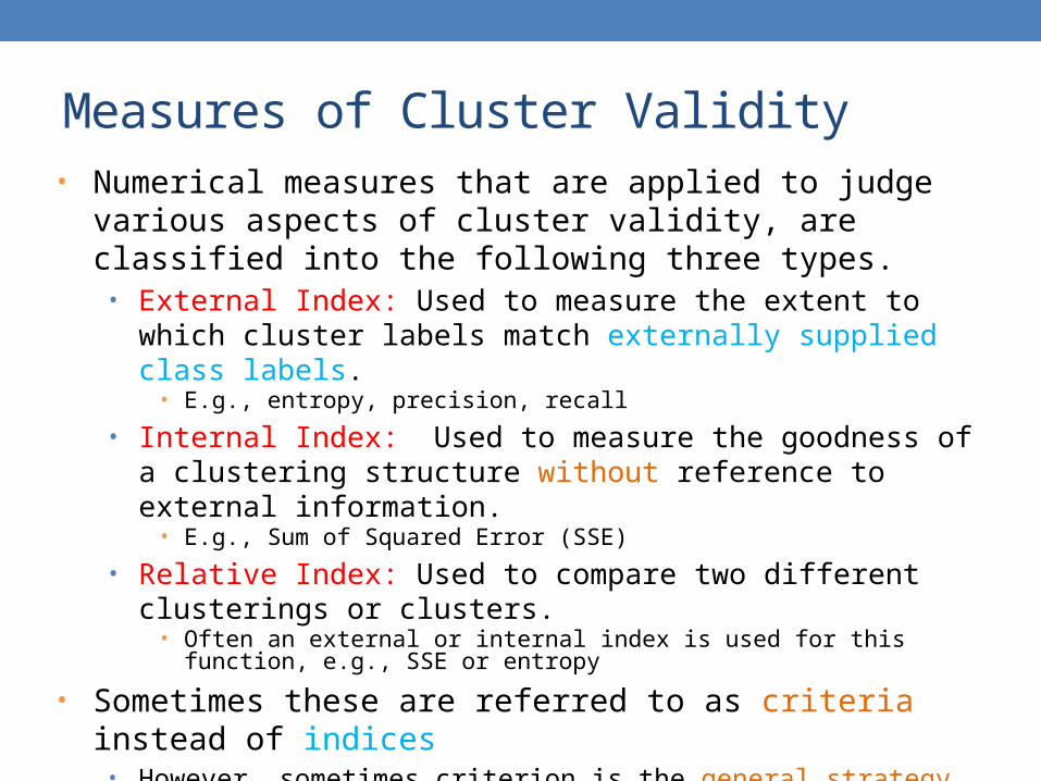
• Numerical measures that are applied to judge various aspects of cluster validity, are classified into the following three types.• External Index: Used to measure the extent to which cluster labels
match externally supplied class labels.• E.g., entropy, precision, recall
• Internal Index: Used to measure the goodness of a clustering structure without reference to external information.
• E.g., Sum of Squared Error (SSE)
• Relative Index: Used to compare two different clusterings or clusters.
• Often an external or internal index is used for this function, e.g., SSE or entropy
• Sometimes these are referred to as criteria instead of indices• However, sometimes criterion is the general strategy and index is the
numerical measure that implements the criterion.
Measures of Cluster Validity
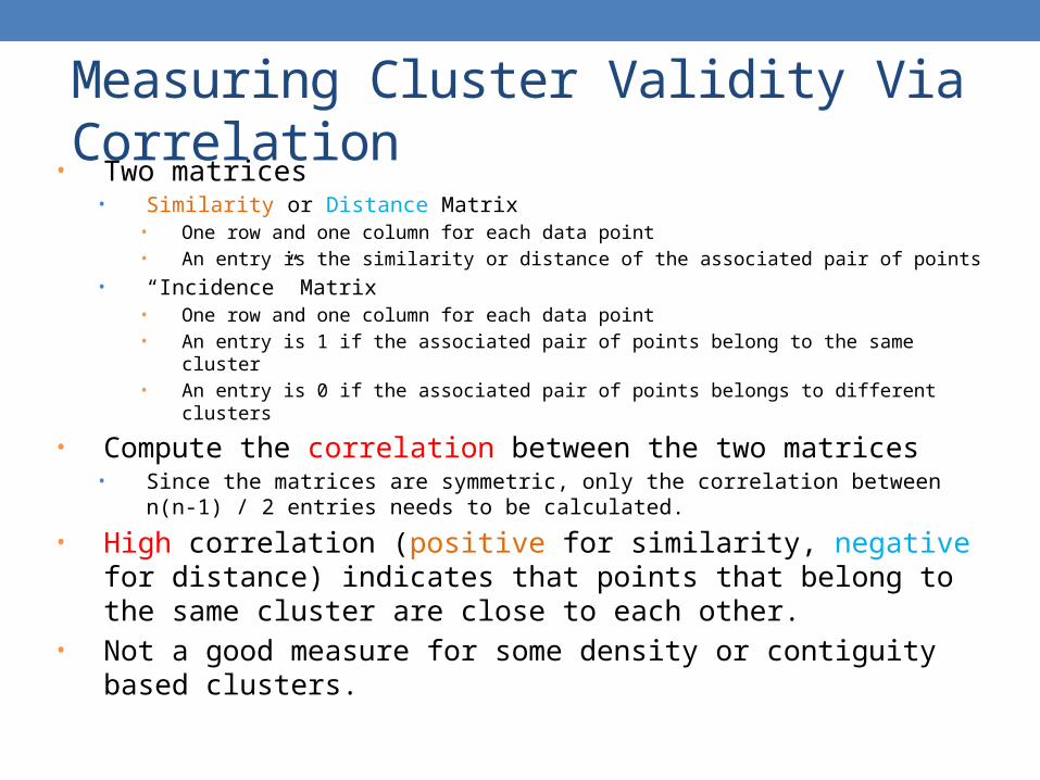
• Two matrices • Similarity or Distance Matrix
• One row and one column for each data point• An entry is the similarity or distance of the associated pair of points
• “Incidence” Matrix• One row and one column for each data point• An entry is 1 if the associated pair of points belong to the same cluster• An entry is 0 if the associated pair of points belongs to different clusters
• Compute the correlation between the two matrices• Since the matrices are symmetric, only the correlation between
n(n-1) / 2 entries needs to be calculated.
• High correlation (positive for similarity, negative for distance) indicates that points that belong to the same cluster are close to each other.
• Not a good measure for some density or contiguity based clusters.
Measuring Cluster Validity Via Correlation

Measuring Cluster Validity Via Correlation
• Correlation of incidence and proximity matrices for the K-means clusterings of the following two data sets.
0 0.2 0.4 0.6 0.8 10
0.1
0.2
0.3
0.4
0.5
0.6
0.7
0.8
0.9
1
x
y
0 0.2 0.4 0.6 0.8 10
0.1
0.2
0.3
0.4
0.5
0.6
0.7
0.8
0.9
1
x
y
Corr = -0.9235 Corr = -0.5810
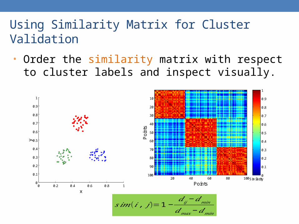
• Order the similarity matrix with respect to cluster labels and inspect visually.
Using Similarity Matrix for Cluster Validation
0 0.2 0.4 0.6 0.8 10
0.1
0.2
0.3
0.4
0.5
0.6
0.7
0.8
0.9
1
x
y
Points
Po
ints
20 40 60 80 100
10
20
30
40
50
60
70
80
90
100Similarity
0
0.1
0.2
0.3
0.4
0.5
0.6
0.7
0.8
0.9
1
𝑠𝑖𝑚(𝑖 , 𝑗)=1−𝑑𝑖𝑗 −𝑑𝑚𝑖𝑛
𝑑𝑚𝑎𝑥 −𝑑𝑚𝑖𝑛
Using Similarity Matrix for Cluster Validation
• Clusters in random data are not so crisp
Points
Po
ints
20 40 60 80 100
10
20
30
40
50
60
70
80
90
100Similarity
0
0.1
0.2
0.3
0.4
0.5
0.6
0.7
0.8
0.9
1
DBSCAN
0 0.2 0.4 0.6 0.8 10
0.1
0.2
0.3
0.4
0.5
0.6
0.7
0.8
0.9
1
xy
Points
Po
ints
20 40 60 80 100
10
20
30
40
50
60
70
80
90
100Similarity
0
0.1
0.2
0.3
0.4
0.5
0.6
0.7
0.8
0.9
1
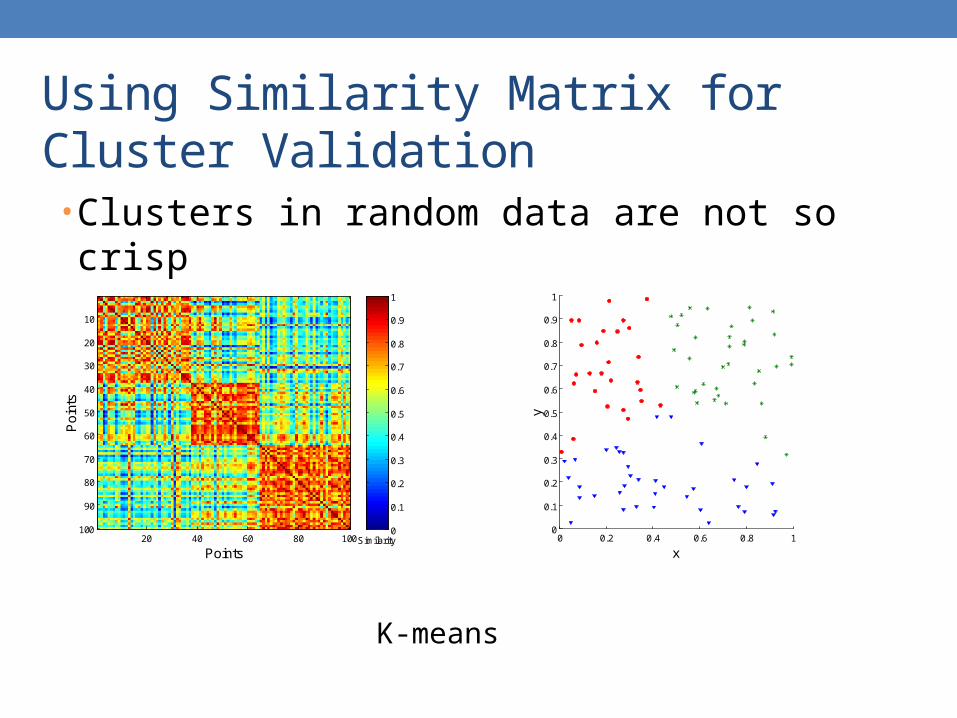
Using Similarity Matrix for Cluster Validation
• Clusters in random data are not so crisp
K-means
0 0.2 0.4 0.6 0.8 10
0.1
0.2
0.3
0.4
0.5
0.6
0.7
0.8
0.9
1
xy
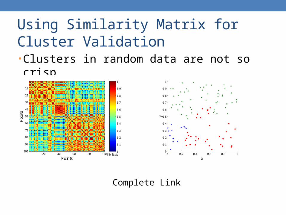
Using Similarity Matrix for Cluster Validation• Clusters in random data are not so crisp
0 0.2 0.4 0.6 0.8 10
0.1
0.2
0.3
0.4
0.5
0.6
0.7
0.8
0.9
1
xy
Points
Po
ints
20 40 60 80 100
10
20
30
40
50
60
70
80
90
100Similarity
0
0.1
0.2
0.3
0.4
0.5
0.6
0.7
0.8
0.9
1
Complete Link
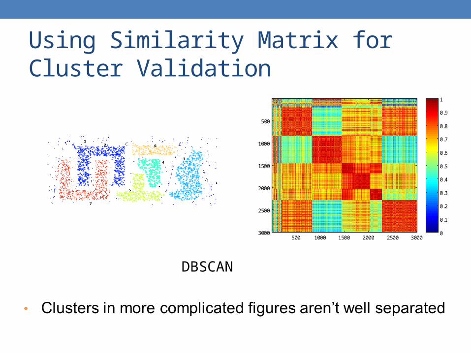
Using Similarity Matrix for Cluster Validation
1 2
3
5
6
4
7
DBSCAN
0
0.1
0.2
0.3
0.4
0.5
0.6
0.7
0.8
0.9
1
500 1000 1500 2000 2500 3000
500
1000
1500
2000
2500
3000
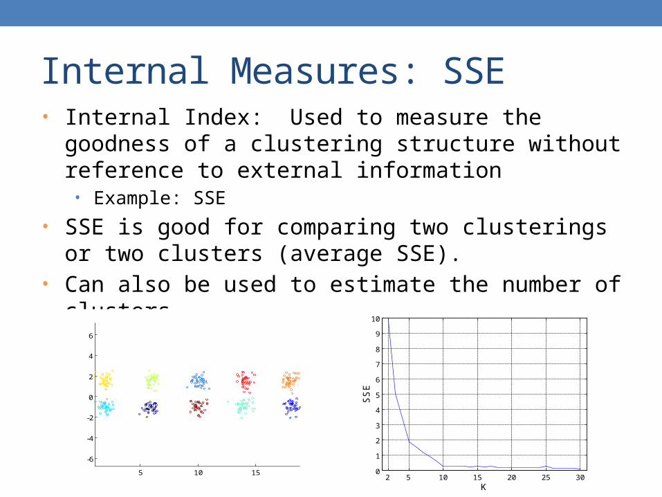
• Internal Index: Used to measure the goodness of a clustering structure without reference to external information• Example: SSE
• SSE is good for comparing two clusterings or two clusters (average SSE).
• Can also be used to estimate the number of clusters
Internal Measures: SSE
2 5 10 15 20 25 300
1
2
3
4
5
6
7
8
9
10
K
SS
E
5 10 15
-6
-4
-2
0
2
4
6

Estimating the “right” number of clusters
• Typical approach: find a “knee” in an internal measure curve.
• Question: why not the k that minimizes the SSE?• Forward reference: minimize a measure, but with a “simple” clustering
• Desirable property: the clustering algorithm does not require the number of clusters to be specified (e.g., DBSCAN)
2 5 10 15 20 25 300
1
2
3
4
5
6
7
8
9
10
K
SS
E
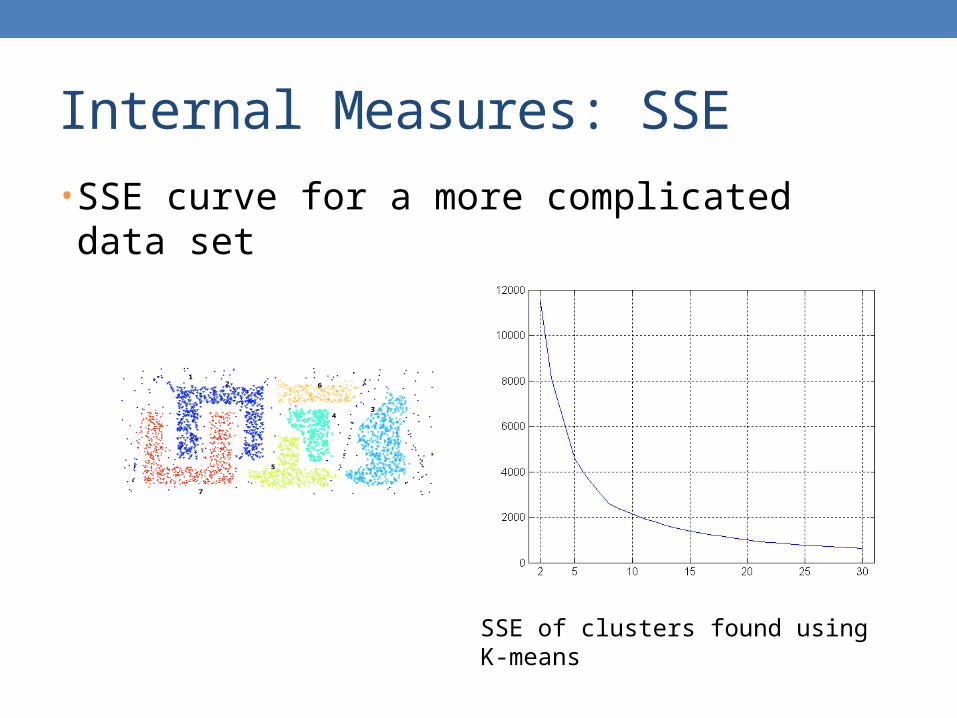
Internal Measures: SSE
• SSE curve for a more complicated data set
1 2
3
5
6
4
7
SSE of clusters found using K-means
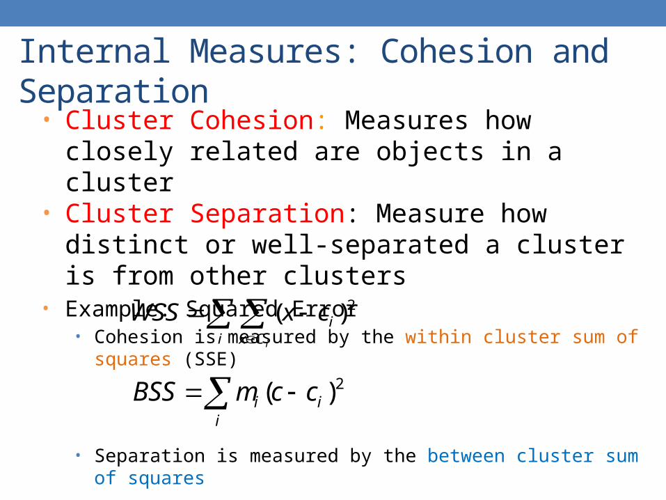
• Cluster Cohesion: Measures how closely related are objects in a cluster
• Cluster Separation: Measure how distinct or well-separated a cluster is from other clusters
• Example: Squared Error• Cohesion is measured by the within cluster sum of squares (SSE)
• Separation is measured by the between cluster sum of squares
• Where mi is the size of cluster i
Internal Measures: Cohesion and Separation
i Cx
i
i
cxWSS 2)(
i
ii ccmBSS 2)(
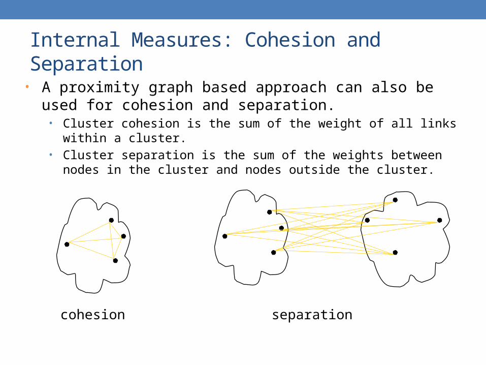
• A proximity graph based approach can also be used for cohesion and separation.
• Cluster cohesion is the sum of the weight of all links within a cluster.• Cluster separation is the sum of the weights between nodes in the cluster
and nodes outside the cluster.
Internal Measures: Cohesion and Separation
cohesion separation
Internal measures – caveats
• Internal measures have the problem that the clustering algorithm did not set out to optimize this measure, so it is will not necessarily do well with respect to the measure.
• An internal measure can also be used as an objective function for clustering
• Need a framework to interpret any measure. • For example, if our measure of evaluation has the value, 10, is that
good, fair, or poor?
• Statistics provide a framework for cluster validity• The more “non-random” a clustering result is, the more likely it
represents valid structure in the data• Can compare the values of an index that result from random data or
clusterings to those of a clustering result.• If the value of the index is unlikely, then the cluster results are valid
• For comparing the results of two different sets of cluster analyses, a framework is less necessary.
• However, there is the question of whether the difference between two index values is significant
Framework for Cluster Validity

• Example• Compare SSE of 0.005 against three clusters in random data• Histogram of SSE for three clusters in 500 random data sets of
100 random points distributed in the range 0.2 – 0.8 for x and y• Value 0.005 is very unlikely
Statistical Framework for SSE
0.016 0.018 0.02 0.022 0.024 0.026 0.028 0.03 0.032 0.0340
5
10
15
20
25
30
35
40
45
50
SSE
Co
unt
0 0.2 0.4 0.6 0.8 10
0.1
0.2
0.3
0.4
0.5
0.6
0.7
0.8
0.9
1
x
y
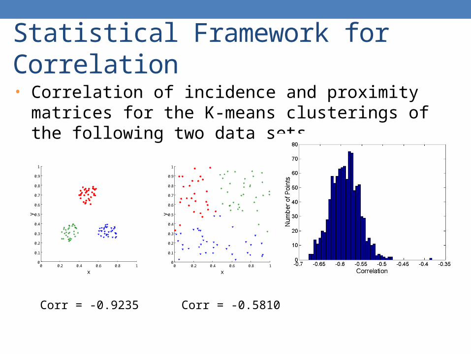
• Correlation of incidence and proximity matrices for the K-means clusterings of the following two data sets.
Statistical Framework for Correlation
0 0.2 0.4 0.6 0.8 10
0.1
0.2
0.3
0.4
0.5
0.6
0.7
0.8
0.9
1
x
y
0 0.2 0.4 0.6 0.8 10
0.1
0.2
0.3
0.4
0.5
0.6
0.7
0.8
0.9
1
x
y
Corr = -0.9235 Corr = -0.5810
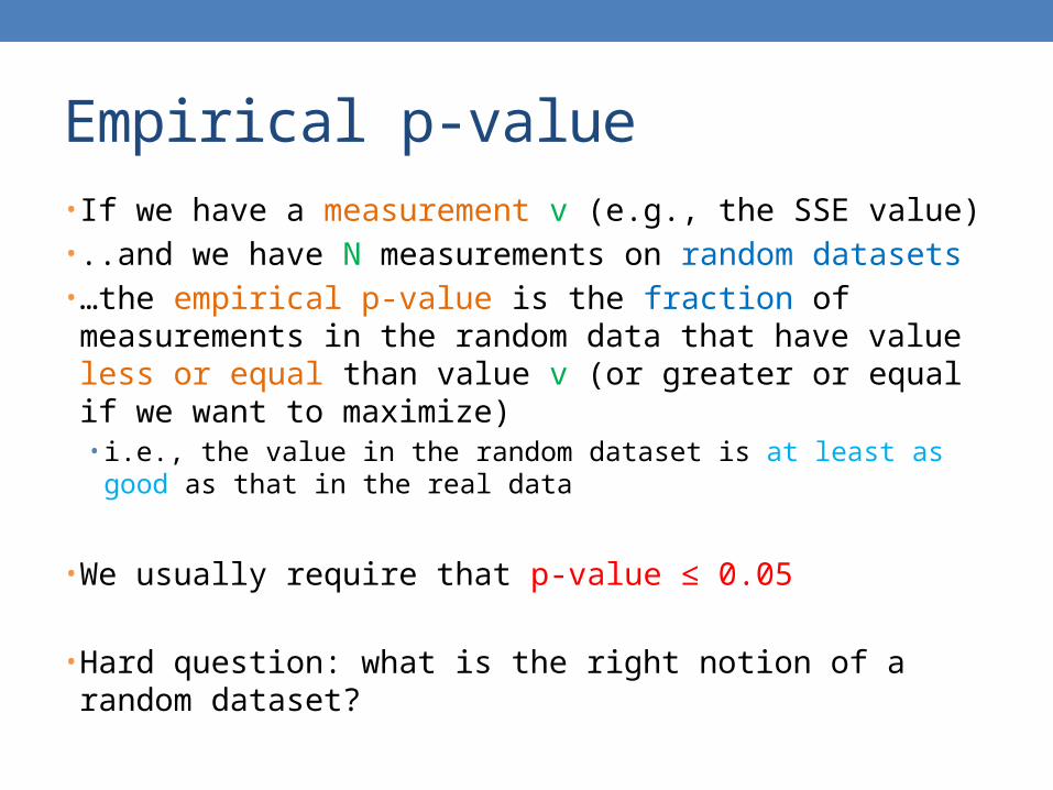
Empirical p-value• If we have a measurement v (e.g., the SSE value)• ..and we have N measurements on random datasets• …the empirical p-value is the fraction of measurements
in the random data that have value less or equal than value v (or greater or equal if we want to maximize) • i.e., the value in the random dataset is at least as good as that
in the real data
• We usually require that p-value ≤ 0.05
• Hard question: what is the right notion of a random dataset?
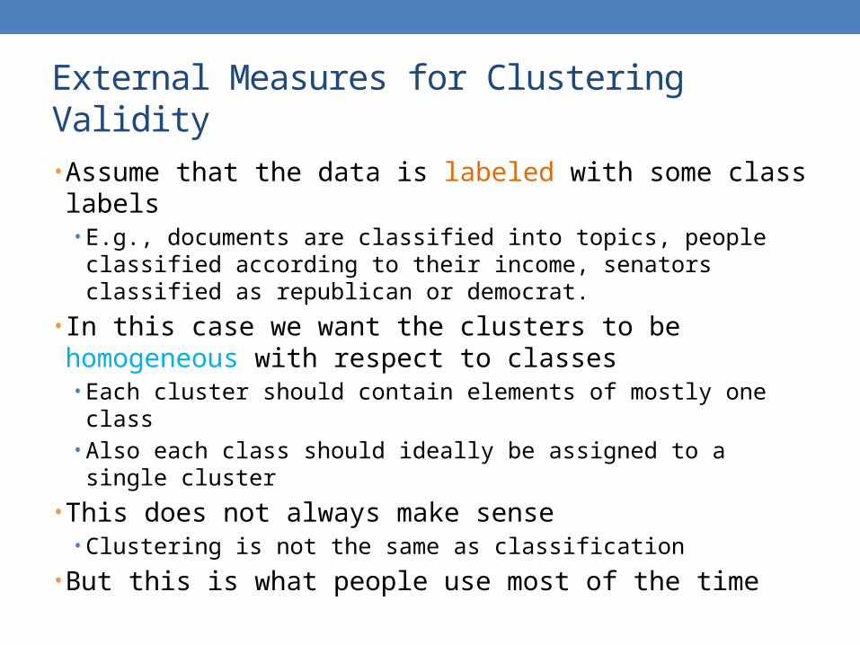
External Measures for Clustering Validity
• Assume that the data is labeled with some class labels• E.g., documents are classified into topics, people classified
according to their income, senators classified as republican or democrat.
• In this case we want the clusters to be homogeneous with respect to classes• Each cluster should contain elements of mostly one class• Also each class should ideally be assigned to a single cluster
• This does not always make sense• Clustering is not the same as classification
• But this is what people use most of the time

Measures• = number of points• = points in cluster i• = points in class j• = points in cluster i coming from
class j• = prob of element from class j in
cluster i• Entropy:
• Of a cluster i: • Highest when uniform, zero when single
class
• Of a clustering:
• Purity:• Of a cluster i: • Of a clustering:
Class 1 Class 2 Class 3
Cluster 1
Cluster 2
Cluster 3
Measures
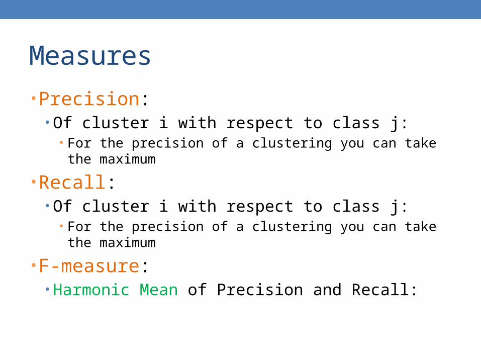
• Precision:• Of cluster i with respect to class j:
• For the precision of a clustering you can take the maximum
• Recall:• Of cluster i with respect to class j:
• For the precision of a clustering you can take the maximum
• F-measure:• Harmonic Mean of Precision and Recall:
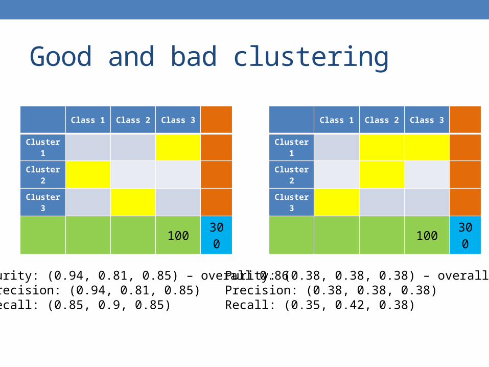
Good and bad clustering
Class 1 Class 2 Class 3
Cluster 1
Cluster 2
Cluster 3
100 300
Class 1 Class 2 Class 3
Cluster 1
Cluster 2
Cluster 3
100 300
Purity: (0.94, 0.81, 0.85) – overall 0.86Precision: (0.94, 0.81, 0.85)Recall: (0.85, 0.9, 0.85)
Purity: (0.38, 0.38, 0.38) – overall 0.38Precision: (0.38, 0.38, 0.38) Recall: (0.35, 0.42, 0.38)
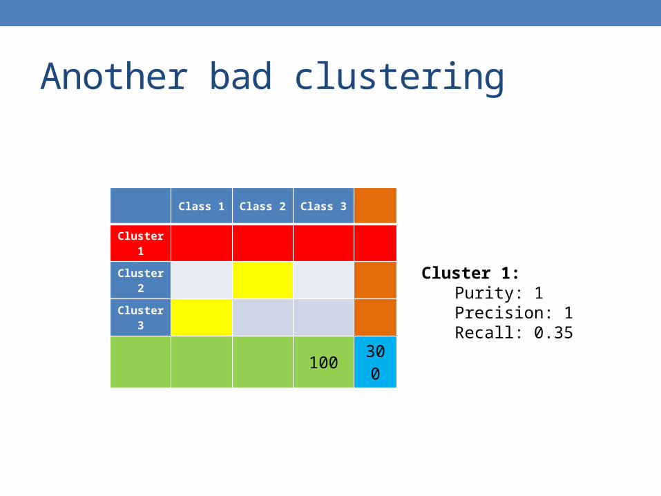
Another bad clustering
Class 1 Class 2 Class 3
Cluster 1
Cluster 2
Cluster 3
100 300
Cluster 1: Purity: 1Precision: 1Recall: 0.35
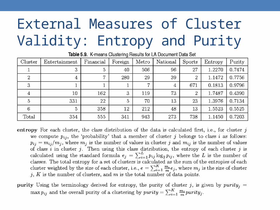
External Measures of Cluster Validity: Entropy and Purity
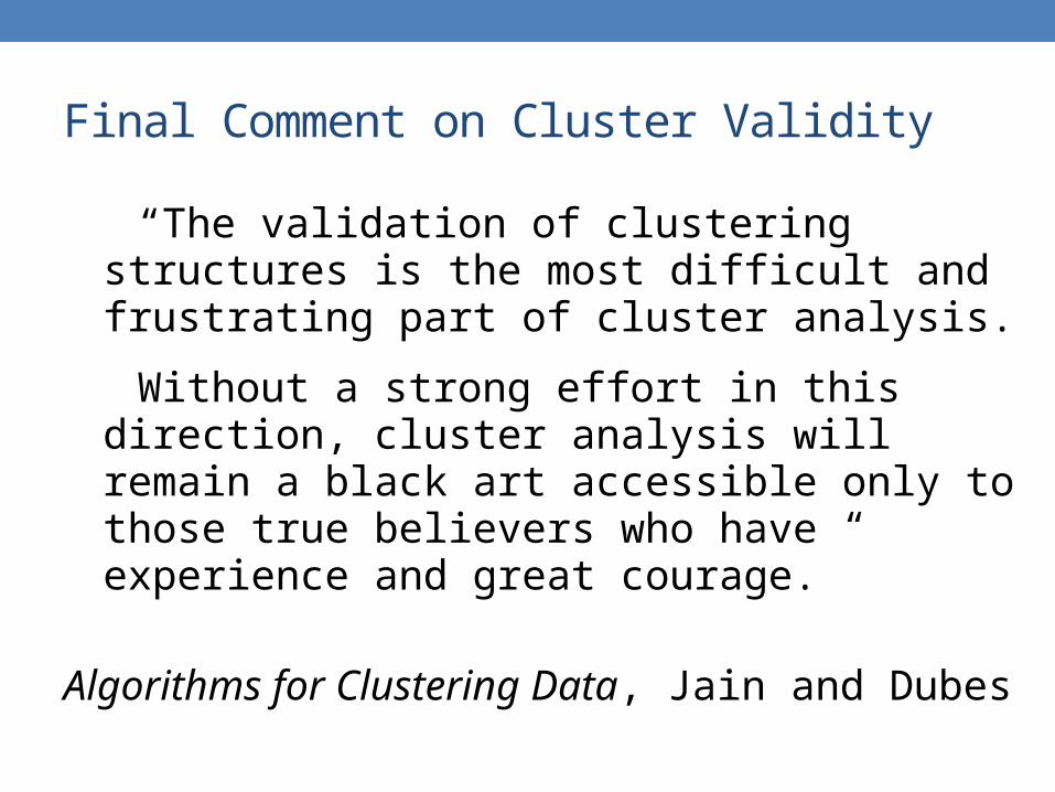
“The validation of clustering structures is the most difficult and frustrating part of cluster analysis.
Without a strong effort in this direction, cluster analysis will remain a black art accessible only to those true believers who have experience and great courage.”
Algorithms for Clustering Data, Jain and Dubes
Final Comment on Cluster Validity

MINIMUM DESCRIPTION LENGTH
Occam’s razor
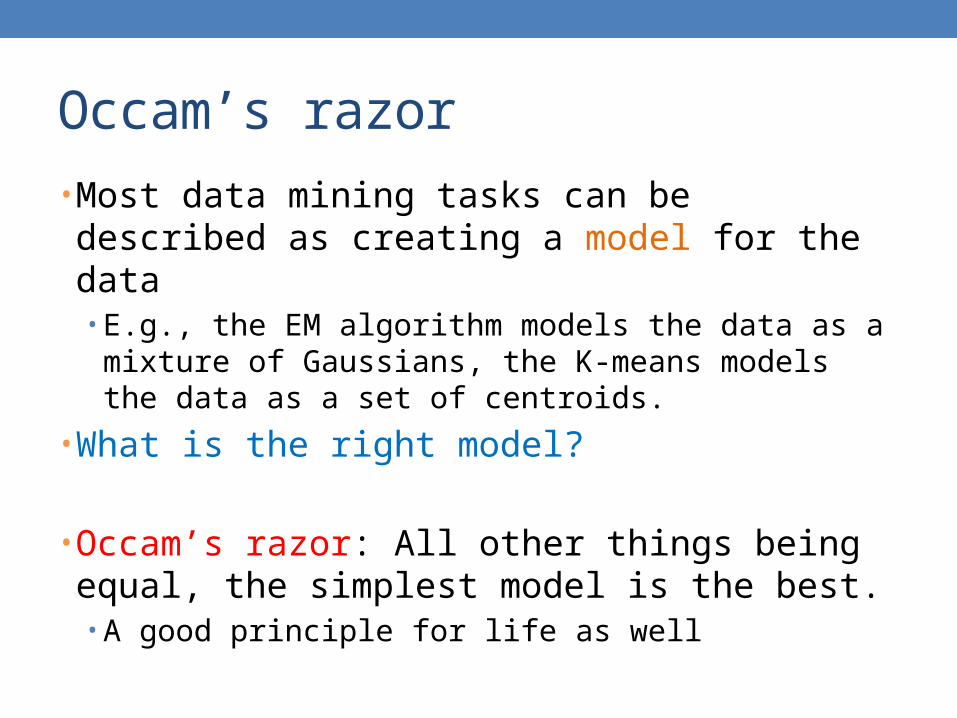
• Most data mining tasks can be described as creating a model for the data• E.g., the EM algorithm models the data as a mixture of
Gaussians, the K-means models the data as a set of centroids.
• What is the right model?
• Occam’s razor: All other things being equal, the simplest model is the best.• A good principle for life as well
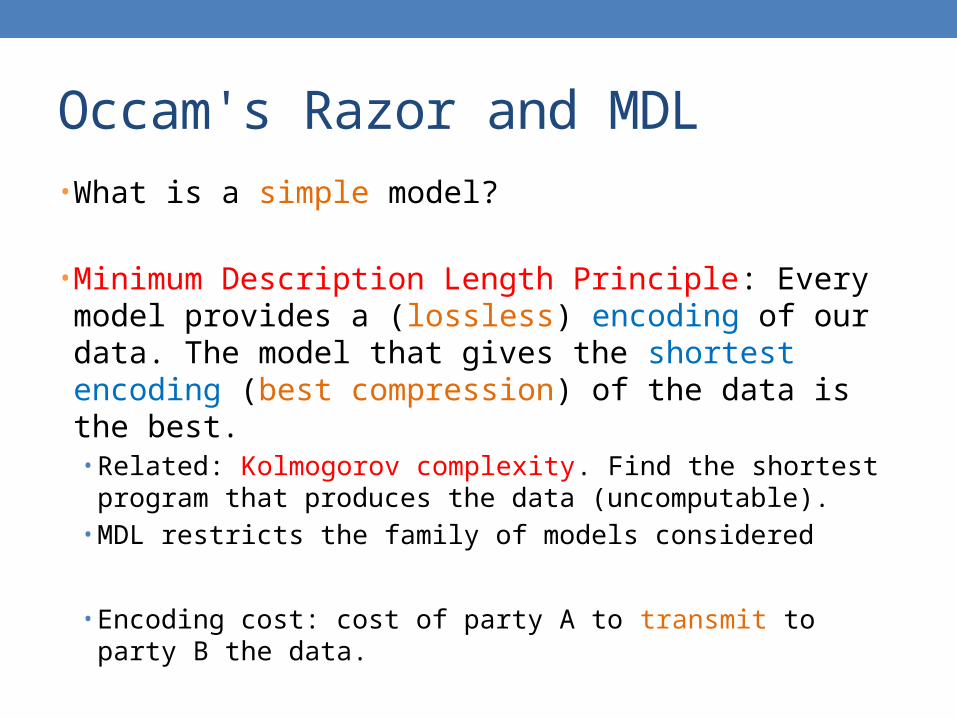
Occam's Razor and MDL
• What is a simple model?
• Minimum Description Length Principle: Every model provides a (lossless) encoding of our data. The model that gives the shortest encoding (best compression) of the data is the best.• Related: Kolmogorov complexity. Find the shortest
program that produces the data (uncomputable). • MDL restricts the family of models considered
• Encoding cost: cost of party A to transmit to party B the data.
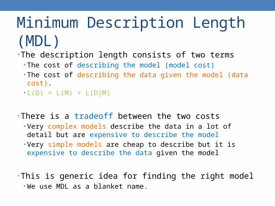
Minimum Description Length (MDL)• The description length consists of two terms
• The cost of describing the model (model cost)• The cost of describing the data given the model (data cost).• L(D) = L(M) + L(D|M)
• There is a tradeoff between the two costs• Very complex models describe the data in a lot of detail but are
expensive to describe the model• Very simple models are cheap to describe but it is expensive to
describe the data given the model
• This is generic idea for finding the right model• We use MDL as a blanket name.
35
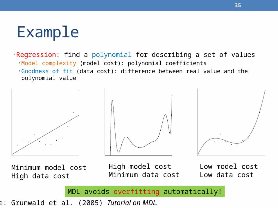
Example• Regression: find a polynomial for describing a set of values
• Model complexity (model cost): polynomial coefficients• Goodness of fit (data cost): difference between real value and the polynomial
value
Source: Grunwald et al. (2005) Tutorial on MDL.
Minimum model costHigh data cost
High model costMinimum data cost
Low model costLow data cost
MDL avoids overfitting automatically!

Example • Suppose you want to describe a set of integer numbers
• Cost of describing a single number is proportional to the value of the number x (e.g., logx).
• How can we get an efficient description?
• Cluster integers into two clusters and describe the cluster by the centroid and the points by their distance from the centroid• Model cost: cost of the centroids• Data cost: cost of cluster membership and distance from centroid
• What are the two extreme cases?
MDL and Data Mining
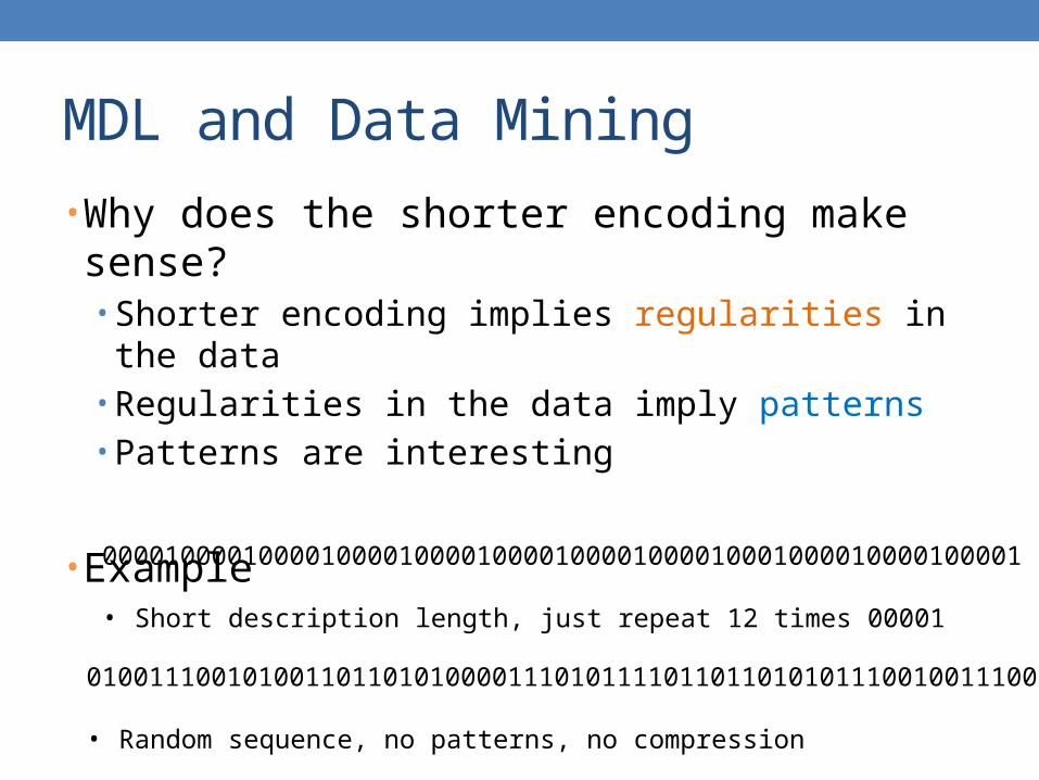
• Why does the shorter encoding make sense?• Shorter encoding implies regularities in the data• Regularities in the data imply patterns• Patterns are interesting
• Example
00001000010000100001000010000100001000010001000010000100001
• Short description length, just repeat 12 times 00001
0100111001010011011010100001110101111011011010101110010011100
• Random sequence, no patterns, no compression

Is everything about compression?• Jürgen Schmidhuber:
A theory about creativity, art and fun• Interesting Art corresponds to a novel pattern that we cannot
compress well, yet it is not too random so we can learn it• Good Humor corresponds to an input that does not
compress well because it is out of place and surprising• Scientific discovery corresponds to a significant
compression event• E.g., a law that can explain all falling apples.
• Fun lecture:• Compression Progress: The Algorithmic Principle Behind Cu
riosity and Creativity

Issues with MDL
• What is the right model family?• This determines the kind of solutions that we can have
• E.g., polynomials • Clusterings
• What is the encoding cost?• Determines the function that we optimize• Information theory

INFORMATION THEORYA short introduction

Encoding
• Consider the following sequence
AAABBBAAACCCABACAABBAACCABAC
• Suppose you wanted to encode it in binary form, how would you do it?
A 0B 10C 11
A is 50% of the sequenceWe should give it a shorter representation
50% A 25% B 25% C
This is actually provably the best encoding!

Encoding• Prefix Codes: no codeword is a prefix of another
• Codes and Distributions: There is one to one mapping between codes and distributions• If P is a distribution over a set of elements (e.g., {A,B,C}) then
there exists a (prefix) code C where • For every (prefix) code C of elements {A,B,C}, we can define a
distribution
• The code defined has the smallest average codelength!
A 0B 10C 11
Uniquely directly decodable
For every code we can find a prefix code of equal length
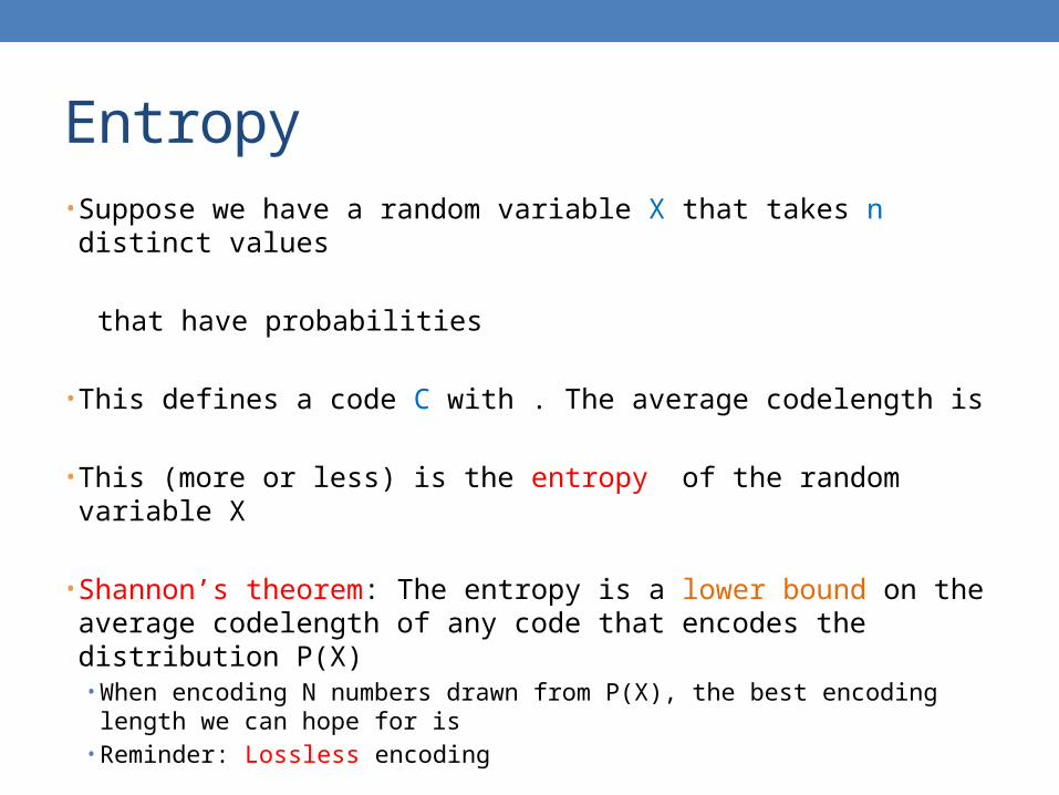
Entropy• Suppose we have a random variable X that takes n distinct values
that have probabilities
• This defines a code C with . The average codelength is
• This (more or less) is the entropy of the random variable X
• Shannon’s theorem: The entropy is a lower bound on the average codelength of any code that encodes the distribution P(X)• When encoding N numbers drawn from P(X), the best encoding length we
can hope for is • Reminder: Lossless encoding
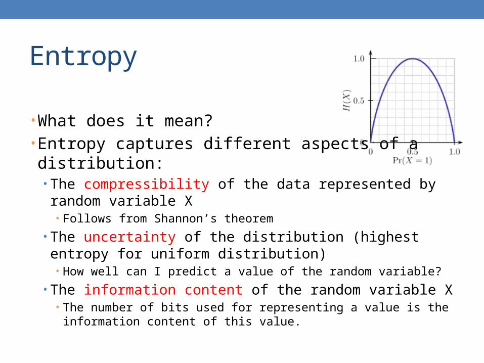
Entropy
• What does it mean?• Entropy captures different aspects of a distribution:
• The compressibility of the data represented by random variable X• Follows from Shannon’s theorem
• The uncertainty of the distribution (highest entropy for uniform distribution)• How well can I predict a value of the random variable?
• The information content of the random variable X• The number of bits used for representing a value is the
information content of this value.

Claude Shannon
Father of Information Theory
Envisioned the idea of communication of information with 0/1 bits
Introduced the word “bit”
The word entropy was suggested by Von Neumann• Similarity to physics, but also • “nobody really knows what entropy really is, so in any
conversation you will have an advantage”

Some information theoretic measures
• Conditional entropy H(Y|X): the uncertainty for Y given that we know X
• Mutual Information I(X,Y): The reduction in the uncertainty for Y (or X) given that we know X (or Y)
Some information theoretic measures
• Cross Entropy: The cost of encoding distribution P, using the code of distribution Q
• KL Divergence KL(P||Q): The increase in encoding cost for distribution P when using the code of distribution Q
• Not symmetric• Problematic if Q not defined for all x of P.
Some information theoretic measures
• Jensen-Shannon Divergence JS(P,Q): distance between two distributions P and Q• Deals with the shortcomings of KL-divergence
• If M = ½ (P+Q) is the mean distribution
• Jensen-Shannon is a metric
USING MDL FOR CO-CLUSTERING(CROSS-ASSOCIATIONS)
Thanks to Spiros Papadimitriou.
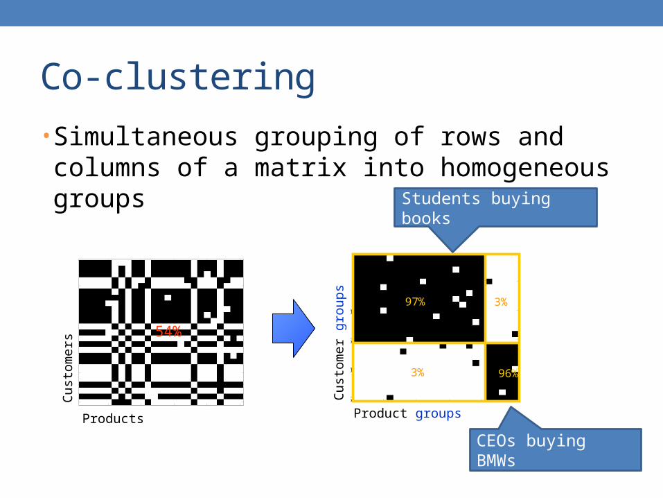
Co-clustering
• Simultaneous grouping of rows and columns of a matrix into homogeneous groups
5 10 15 20 25
5
10
15
20
25
97%
96%
3%
3%
Product groups
Cus
tom
er g
rou
ps
5 10 15 20 25
5
10
15
20
25
Products
54%
Cus
tom
ers
Students buying books
CEOs buying BMWs

Co-clustering
• Step 1: How to define a “good” partitioning?
Intuition and formalization
• Step 2: How to find it?
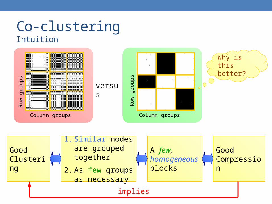
Co-clusteringIntuition
versus
Column groups Column groups
Row
gro
ups
Row
gro
ups
Good Clustering
1. Similar nodes are grouped together
2. As few groups as necessary
A few, homogeneous blocks
Good Compression
Why is this better?
implies
log*k + log*ℓ log nimj
i,j nimj H(pi,j)
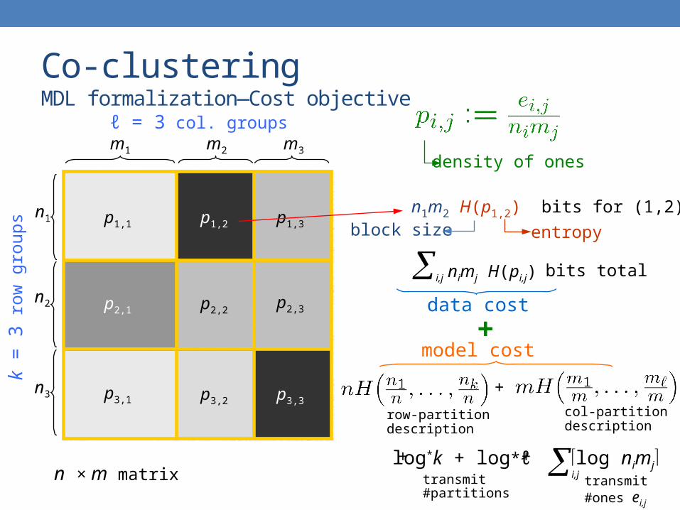
Co-clusteringMDL formalization—Cost objective
n1
n2
n3
m1 m2 m3
p1,1 p1,2 p1,3
p2,1 p2,2 p2,3
p3,3p3,2p3,1
n × m matrix
k =
3 r
ow g
roup
s
ℓ = 3 col. groups
density of ones
n1m2 H(p1,2) bits for (1,2)
data cost
bits total
row-partitiondescription
col-partitiondescription
i,jtransmit#ones ei,j
+
+
model cost+
block size entropy
+transmit#partitions
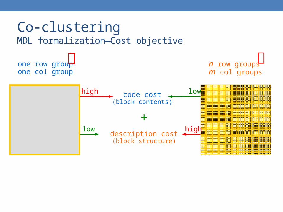
Co-clusteringMDL formalization—Cost objective
code cost(block contents)
description cost(block structure)
+
one row groupone col group
n row groupsm col groups
low
high low
high
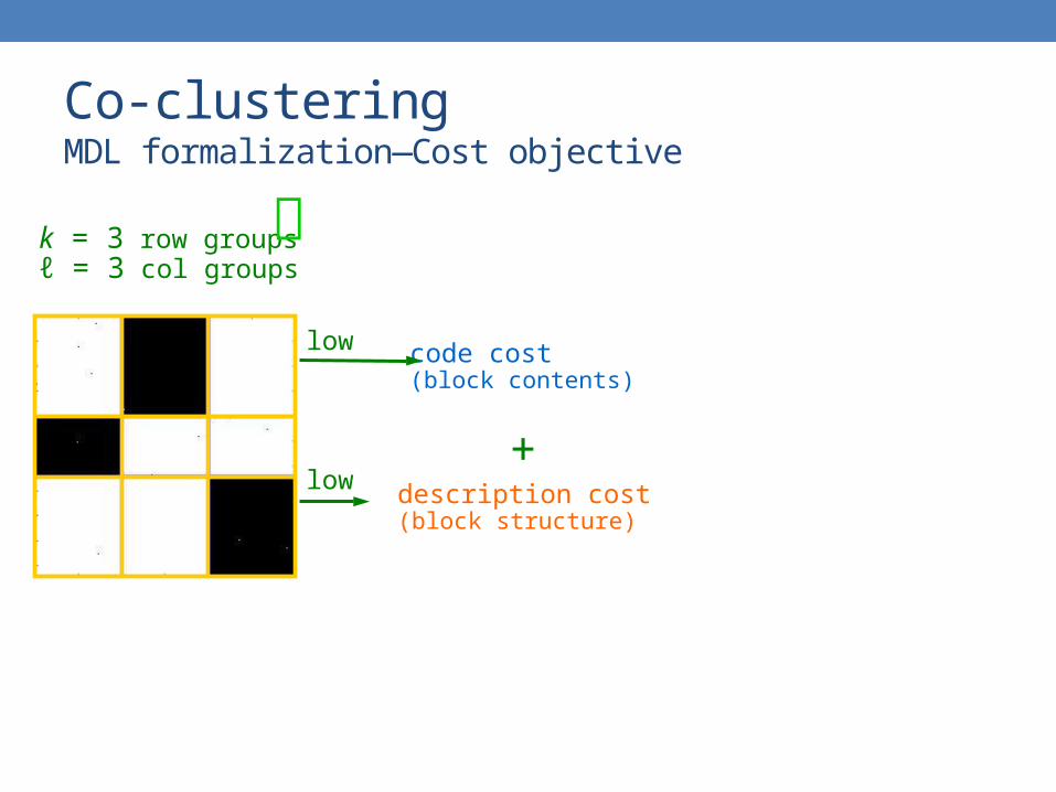
Co-clusteringMDL formalization—Cost objective
code cost(block contents)
description cost(block structure)
+
k = 3 row groupsℓ = 3 col groups
low
low

Co-clusteringMDL formalization—Cost objective
k
ℓ
tota
l bit
cost
Cost vs. number of groups
one row
groupone
col group
n row
groupsm
col g
roupsk =
3 row
groupsℓ =
3 co
l groups
Co-clustering
• Step 1: How to define a “good” partitioning?
Intuition and formalization
• Step 2: How to find it?
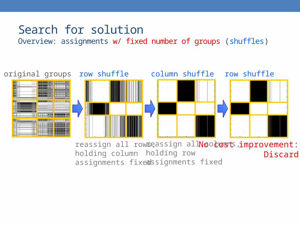
Search for solutionOverview: assignments w/ fixed number of groups (shuffles)
row shuffle column shuffle row shuffleoriginal groups
No cost improvement:Discard
reassign all rows,holding columnassignments fixed
reassign all columns,holding rowassignments fixed
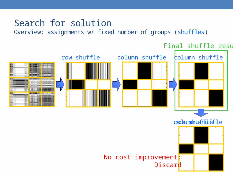
Search for solutionOverview: assignments w/ fixed number of groups (shuffles)
row shuffle column shuffle column shuffle
row shufflecolumn shuffle
No cost improvement:Discard
Final shuffle result

Search for solutionShuffles• Let
denote row and col. partitions at the I-th iteration• Fix I and for every row x:
• Splice into ℓ parts, one for each column group• Let j, for j = 1,…,ℓ, be the number of ones in each part• Assign row x to the row group i¤ I+1(x) such that, for all i
= 1,…,k,
p1,1 p1,2 p1,3
p2,1 p2,2 p2,3
p3,3p3,2p3,1
Similarity (“KL-divergences”)of row fragmentsto blocks of a row group
Assign to second row-group
k = 5, ℓ = 5
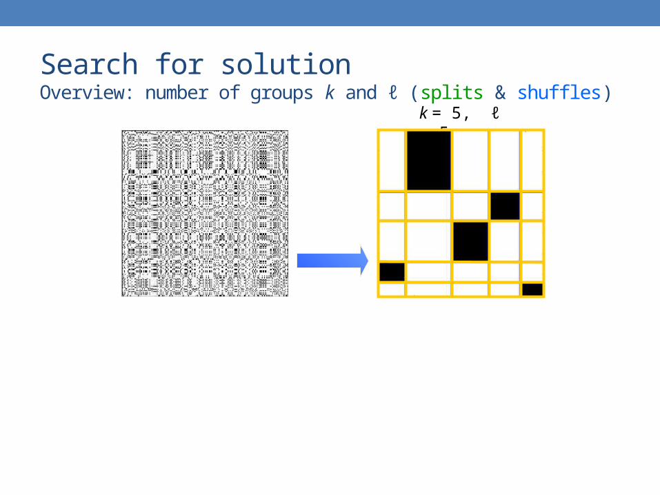
Search for solutionOverview: number of groups k and ℓ (splits & shuffles)

col. splitshuffle
Search for solutionOverview: number of groups k and ℓ (splits & shuffles)
k=1, ℓ=2 k=2, ℓ=2 k=2, ℓ=3 k=3, ℓ=3 k=3, ℓ=4 k=4, ℓ=4 k=4, ℓ=5
k = 1, ℓ = 1
row splitshuffle
Split:Increase k or ℓ
Shuffle:Rearrange rows or cols
col. splitshuffle
row splitshuffle
col. splitshuffle
row splitshuffle
col. splitshuffle
k = 5, ℓ = 5
row splitshuffle
k = 5, ℓ = 6
col. splitshuffle
No cost improvement:Discard
row split
k = 6, ℓ = 5

Search for solutionOverview: number of groups k and ℓ (splits & shuffles)
k=1, ℓ=2 k=2, ℓ=2 k=2, ℓ=3 k=3, ℓ=3 k=3, ℓ=4 k=4, ℓ=4 k=4, ℓ=5
k = 1, ℓ = 1
Split:Increase k or ℓ
Shuffle:Rearrange rows or cols
k = 5, ℓ = 5
k = 5, ℓ = 5
Final result
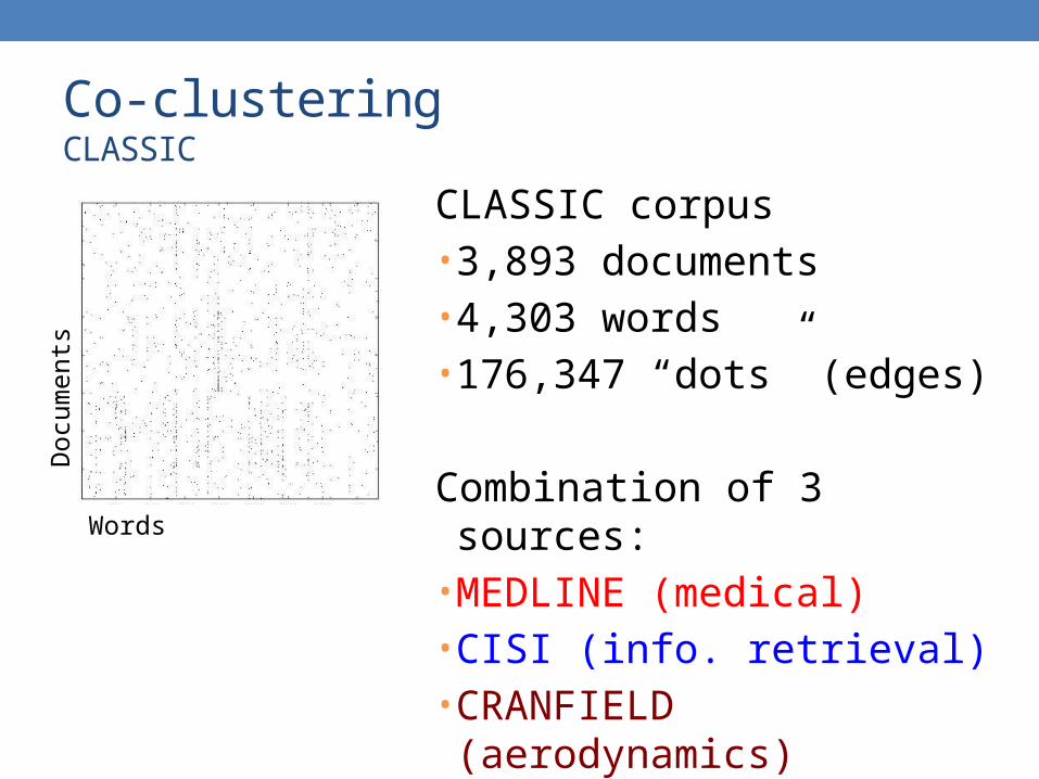
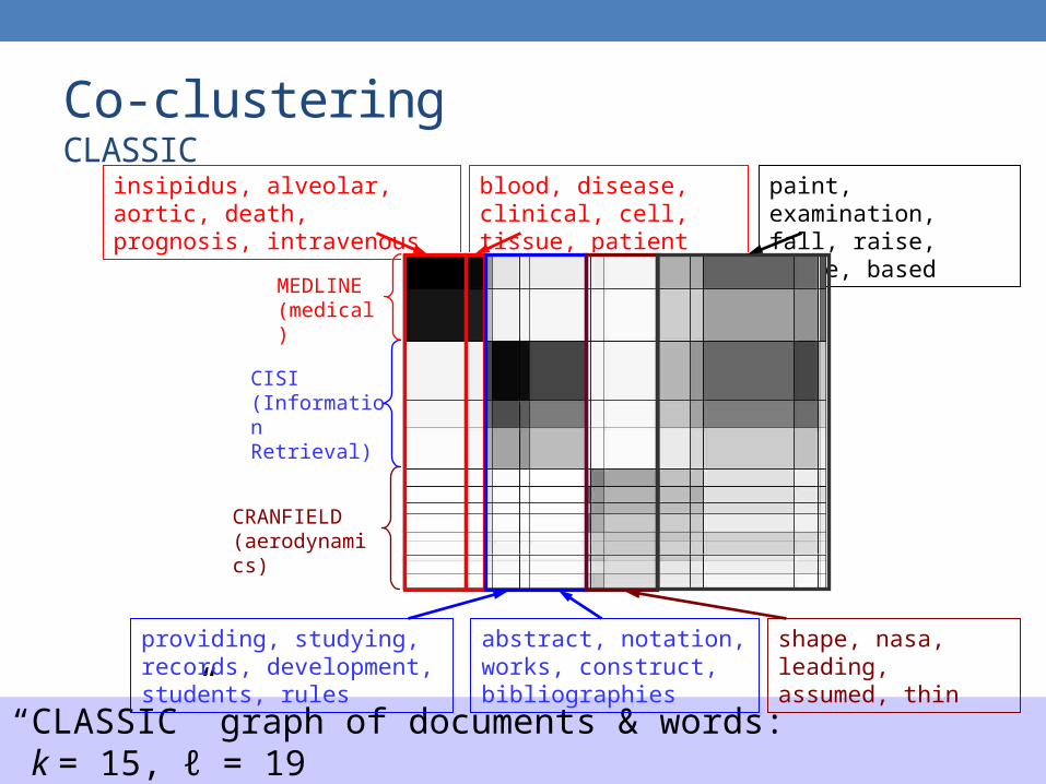
Co-clusteringCLASSIC
CLASSIC corpus• 3,893 documents• 4,303 words• 176,347 “dots” (edges)
Combination of 3 sources:• MEDLINE (medical)• CISI (info. retrieval)• CRANFIELD (aerodynamics)
Doc
umen
ts
Words
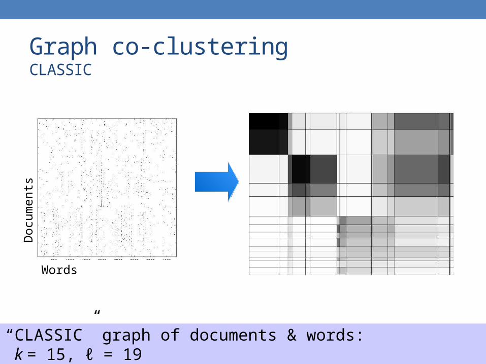
Graph co-clusteringCLASSIC
Doc
umen
ts
Words
“CLASSIC” graph of documents & words: k = 15, ℓ = 19
Co-clusteringCLASSIC
MEDLINE(medical)
insipidus, alveolar, aortic, death, prognosis, intravenous
blood, disease, clinical, cell, tissue, patient
“CLASSIC” graph of documents & words: k = 15, ℓ = 19
CISI(Information Retrieval)
providing, studying, records, development, students, rules
abstract, notation, works, construct, bibliographies
shape, nasa, leading, assumed, thin
paint, examination, fall, raise, leave, based
CRANFIELD (aerodynamics)
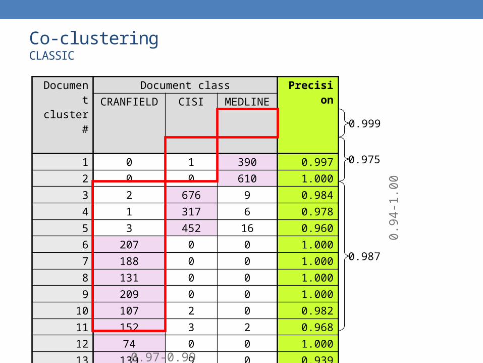
Co-clusteringCLASSIC
Document cluster #
Document class Precision
CRANFIELD CISI MEDLINE
1 0 1 390 0.9972 0 0 610 1.0003 2 676 9 0.9844 1 317 6 0.9785 3 452 16 0.9606 207 0 0 1.0007 188 0 0 1.0008 131 0 0 1.0009 209 0 0 1.000
10 107 2 0 0.98211 152 3 2 0.96812 74 0 0 1.00013 139 9 0 0.93914 163 0 0 1.00015 24 0 0 1.000
Recall 0.996 0.990 0.968
0.94
-1.0
0
0.97-0.99
0.999
0.975
0.987