Data cleaning & Exploratory data analysis

Seungho Ryu, MD, PhDKanguk Samsung Hospital,Sungkyunkwan University

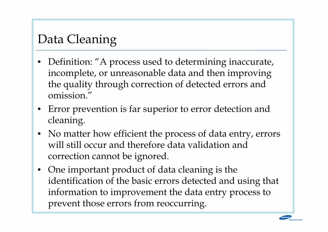
Data Cleaning

• Definition: “A process used to determining inaccurate, incomplete, or unreasonable data and then improving the quality through correction of detected errors and omission.”

• Error prevention is far superior to error detection and cleaning.

• No matter how efficient the process of data entry, errors will still occur and therefore data validation and correction cannot be ignored.

• One important product of data cleaning is the identification of the basic errors detected and using that information to improvement the data entry process to prevent those errors from reoccurring.

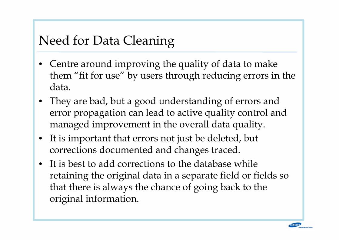
Need for Data Cleaning

• Centre around improving the quality of data to make them “fit for use” by users through reducing errors in the data.

• They are bad, but a good understanding of errors and error propagation can lead to active quality control and managed improvement in the overall data quality.

• It is important that errors not just be deleted, but corrections documented and changes traced.

• It is best to add corrections to the database while retaining the original data in a separate field or fields so that there is always the chance of going back to the original information.

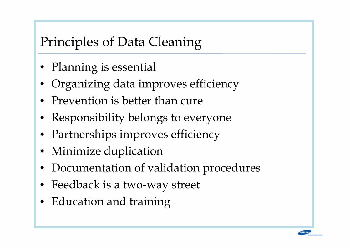
Principles of Data Cleaning

• Planning is essential• Organizing data improves efficiency• Prevention is better than cure• Responsibility belongs to everyone• Partnerships improves efficiency• Minimize duplication• Documentation of validation procedures• Feedback is a two-way street• Education and training

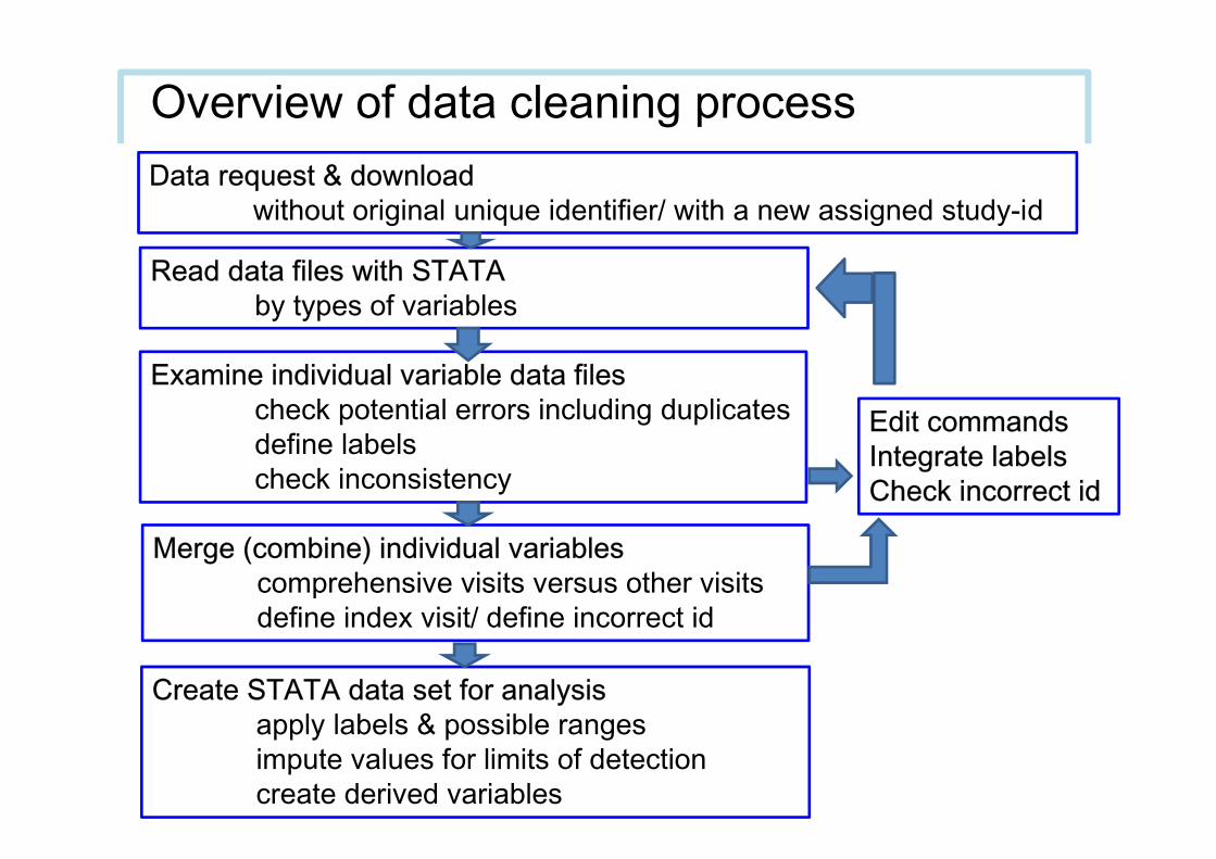
Overview of data cleaning processData request & download

without original unique identifier/ with a new assigned study-id

Read data files with STATAby types of variables

Examine individual variable data files check potential errors including duplicatesdefine labelscheck inconsistency

Merge (combine) individual variablescomprehensive visits versus other visitsdefine index visit/ define incorrect id

Create STATA data set for analysisapply labels & possible rangesimpute values for limits of detectioncreate derived variables

Edit commandsIntegrate labelsCheck incorrect id

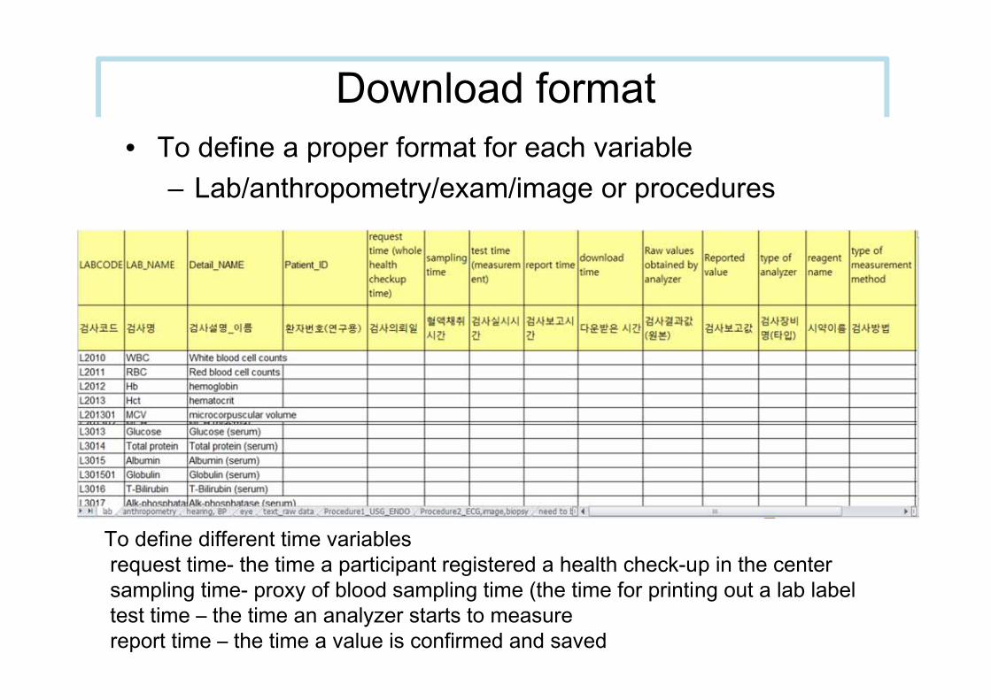
Download format• To define a proper format for each variable

– Lab/anthropometry/exam/image or procedures

To define different time variables request time- the time a participant registered a health check-up in the centersampling time- proxy of blood sampling time (the time for printing out a lab labeltest time – the time an analyzer starts to measurereport time – the time a value is confirmed and saved

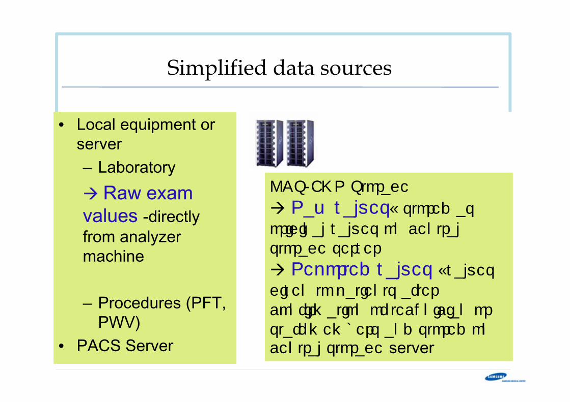
Simplified data sources

OCS/EMR Storage

Raw values– stored as original values on central storage server

Reported values –values given to patients after confirmation of technician or staff members and stored on central storage server

• Local equipment or server– Laboratory

Raw exam values -directly from analyzer machine

– Procedures (PFT, PWV)

• PACS Server

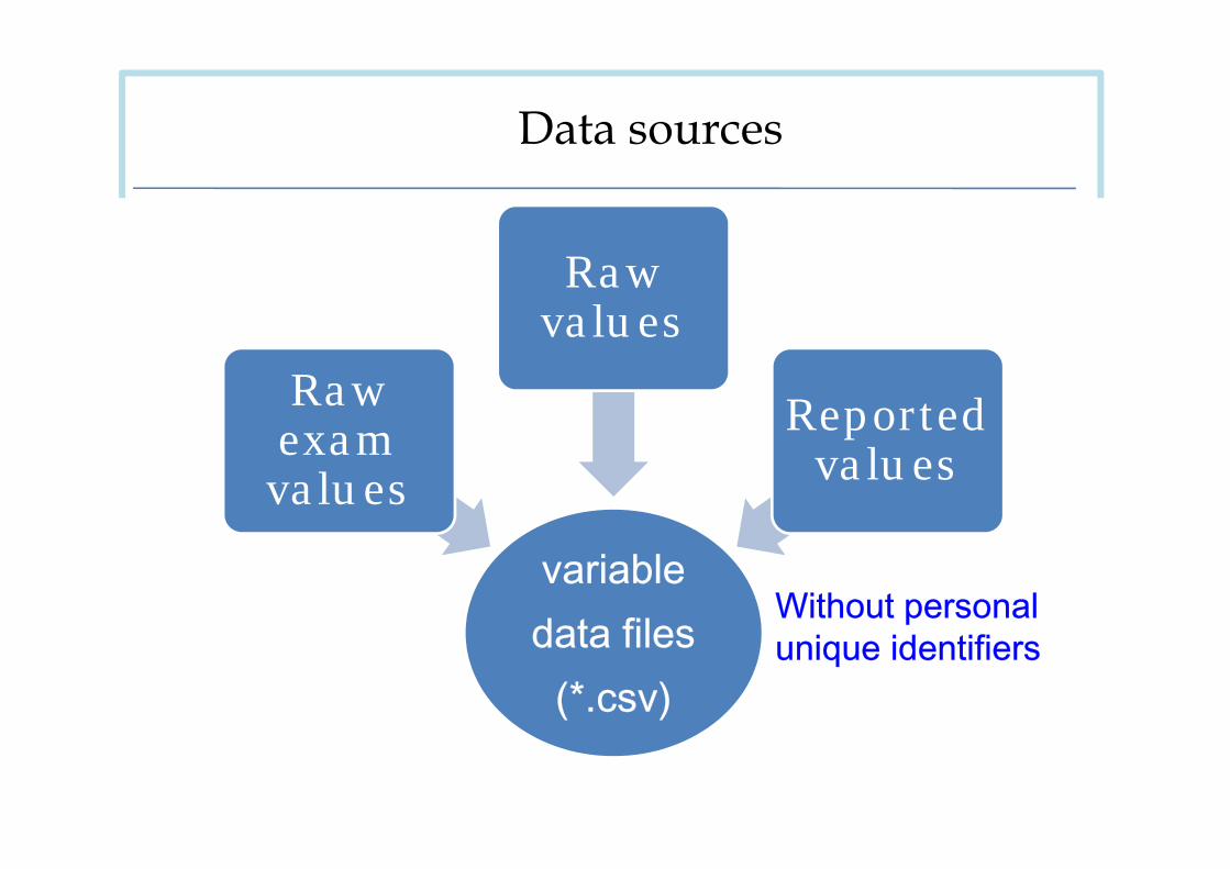
Data sources

variable data files

(*.csv)

Raw exam values

Raw values

Reported values

Without personal unique identifiers

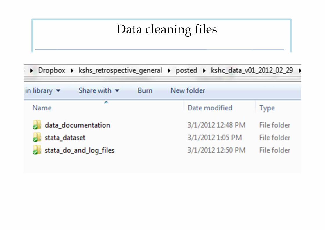
Data cleaning files

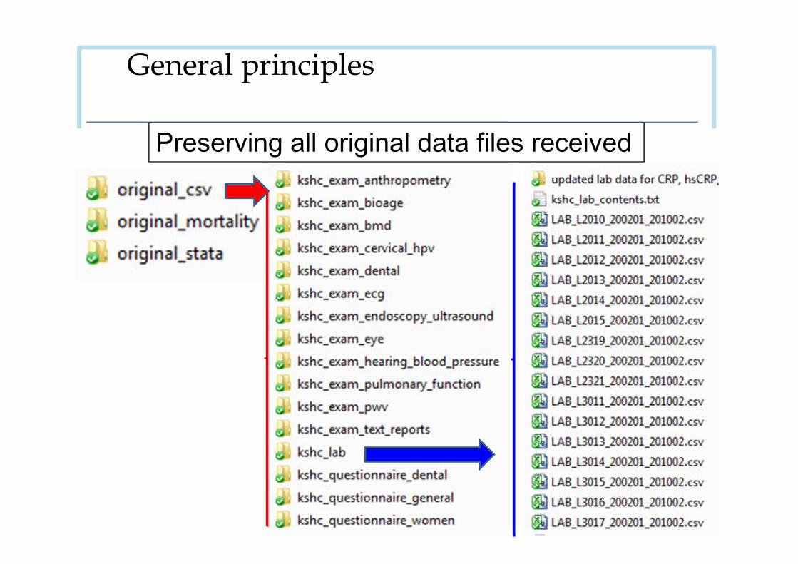
General principles

Preserving all original data files received

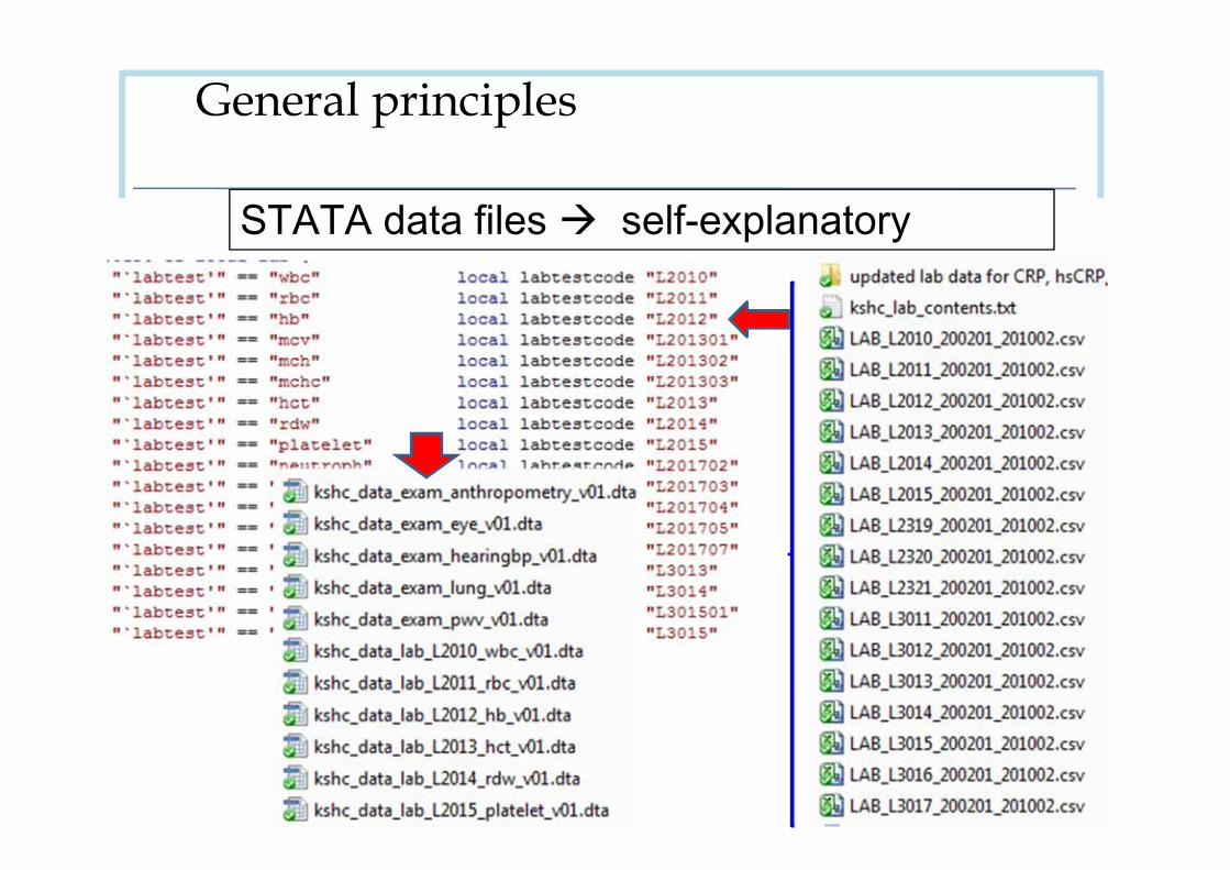
General principles

STATA data files self-explanatory

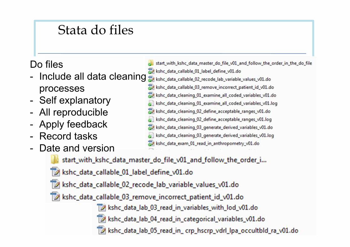
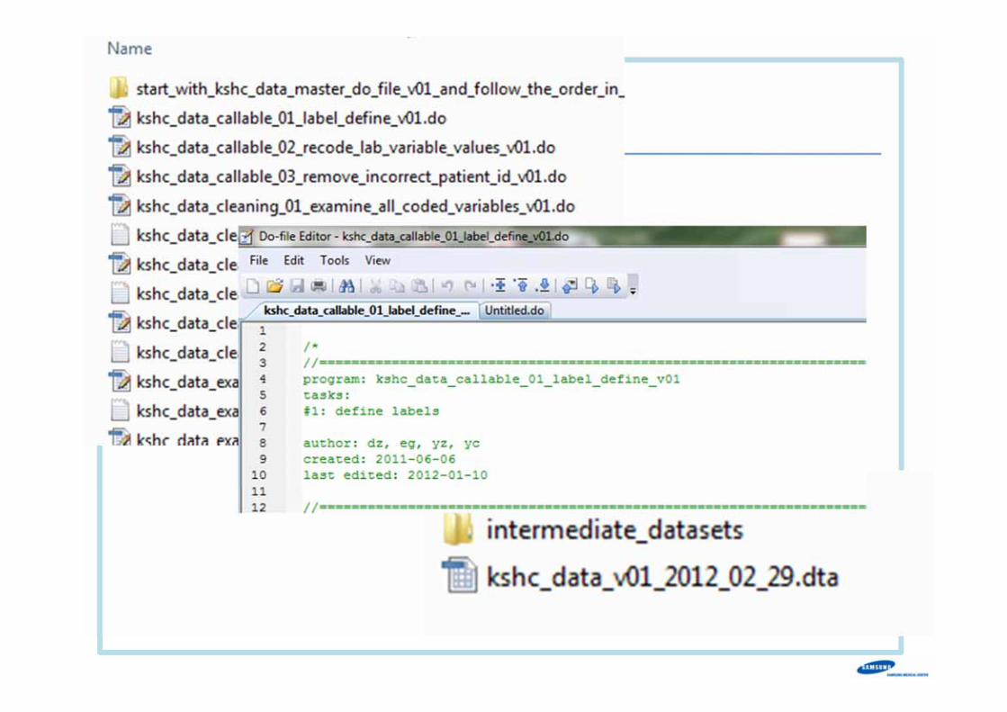
Stata do files

Do files- Include all data cleaning

processes- Self explanatory- All reproducible - Apply feedback- Record tasks- Date and version

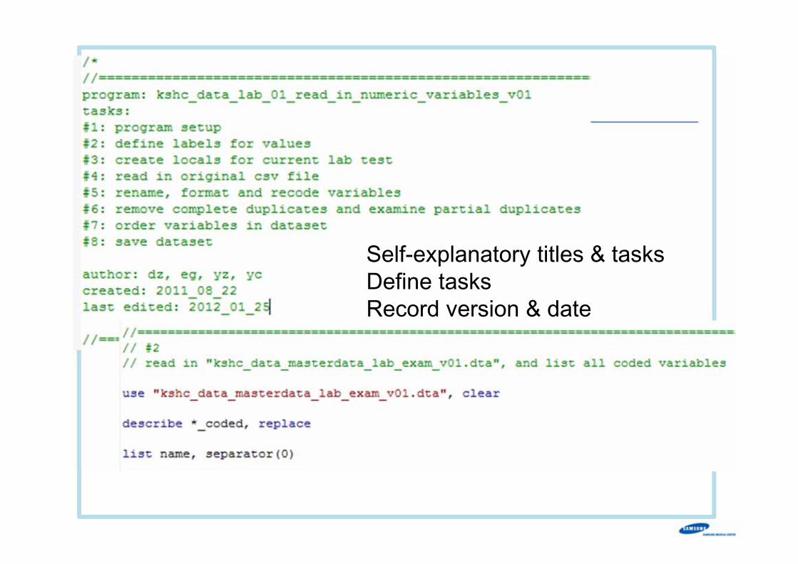
Self-explanatory titles & tasksDefine tasksRecord version & date

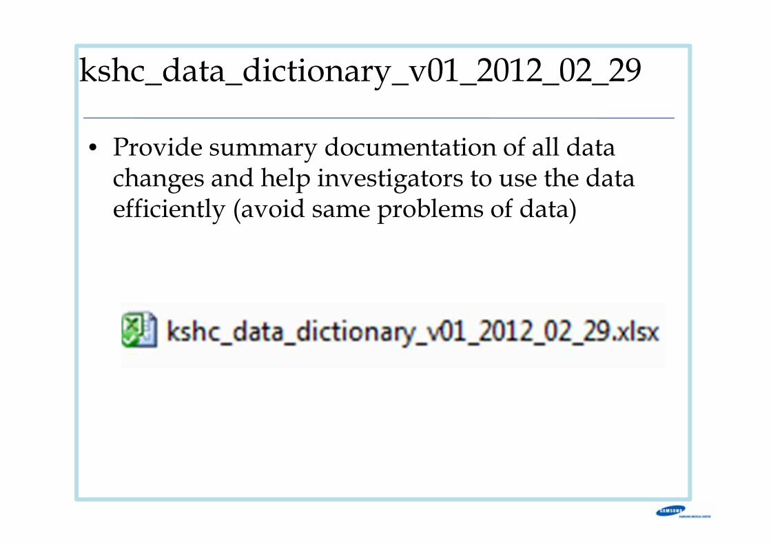
kshc_data_dictionary_v01_2012_02_29

• Provide summary documentation of all data changes and help investigators to use the data efficiently (avoid same problems of data)

Checking data quality & correction

• Checking erroneous values• Range and consistency checks• Developing boundaries for out-of range values –

required a collaborative effort between data cleaning team and clinicians

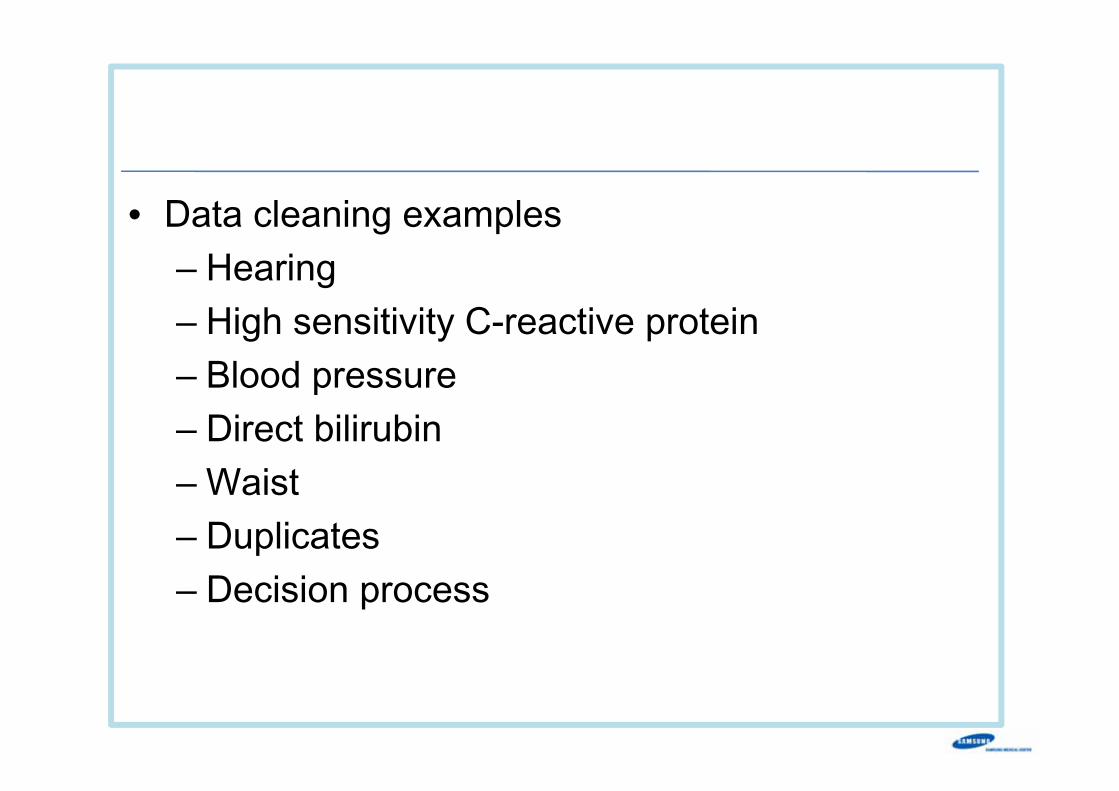
• Data cleaning examples– Hearing – High sensitivity C-reactive protein– Blood pressure– Direct bilirubin– Waist– Duplicates – Decision process

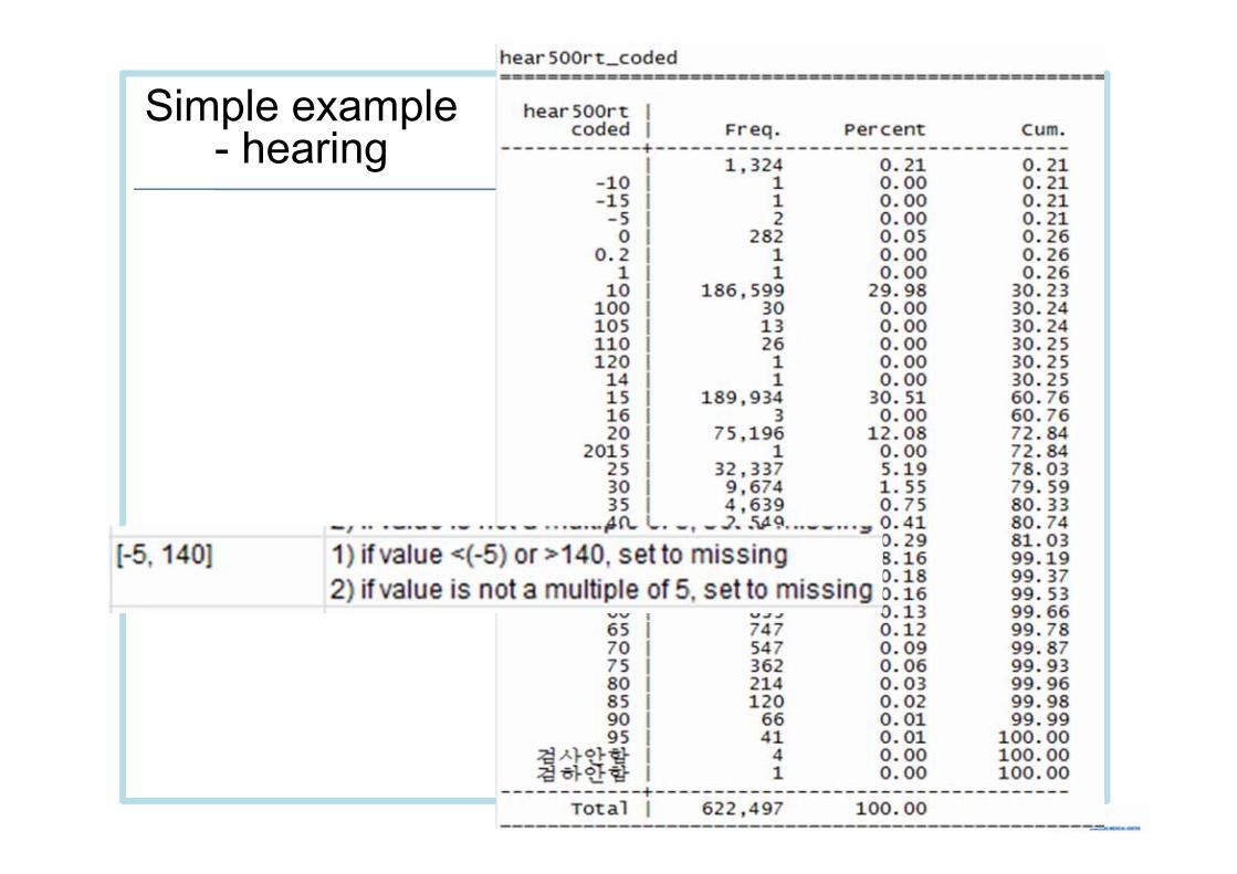
Simple example - hearing

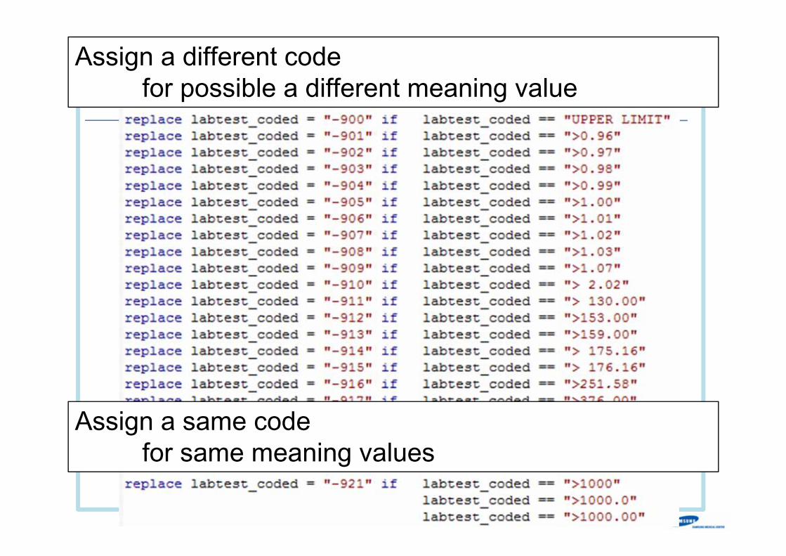
Assign a different code for possible a different meaning value

Assign a same code for same meaning values

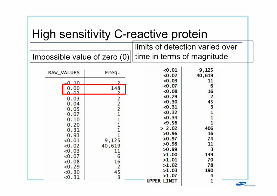
High sensitivity C-reactive protein limits of detection varied over time in terms of magnitudeImpossible value of zero (0)

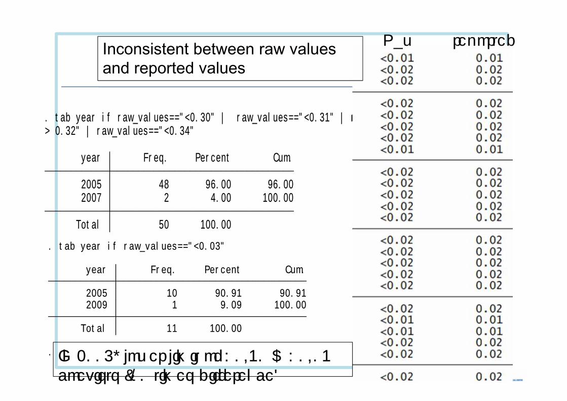
Total 50 100.00 2007 2 4.00 100.00 2005 48 96.00 96.00 year Freq. Percent Cum.

> 0.32" | raw_values=="<0.34". tab year if raw_values=="<0.30" | raw_values=="<0.31" | raw_values=="<

.

Total 11 100.00 2009 1 9.09 100.00 2005 10 90.91 90.91 year Freq. Percent Cum.

. tab year if raw_values=="<0.03"

Inconsistent between raw values and reported values

In 2005, lower limit of <0.30 & <0.03 coexists (10 times difference)

Raw reported

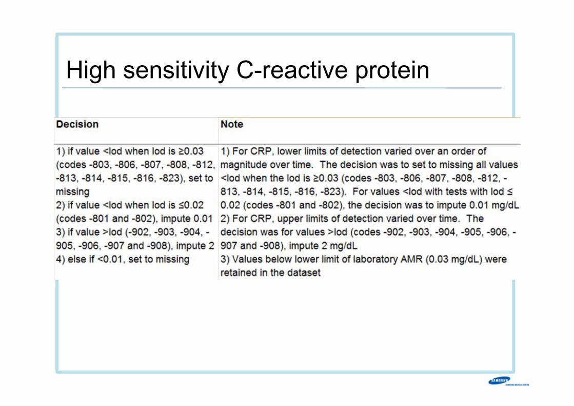
High sensitivity C-reactive protein

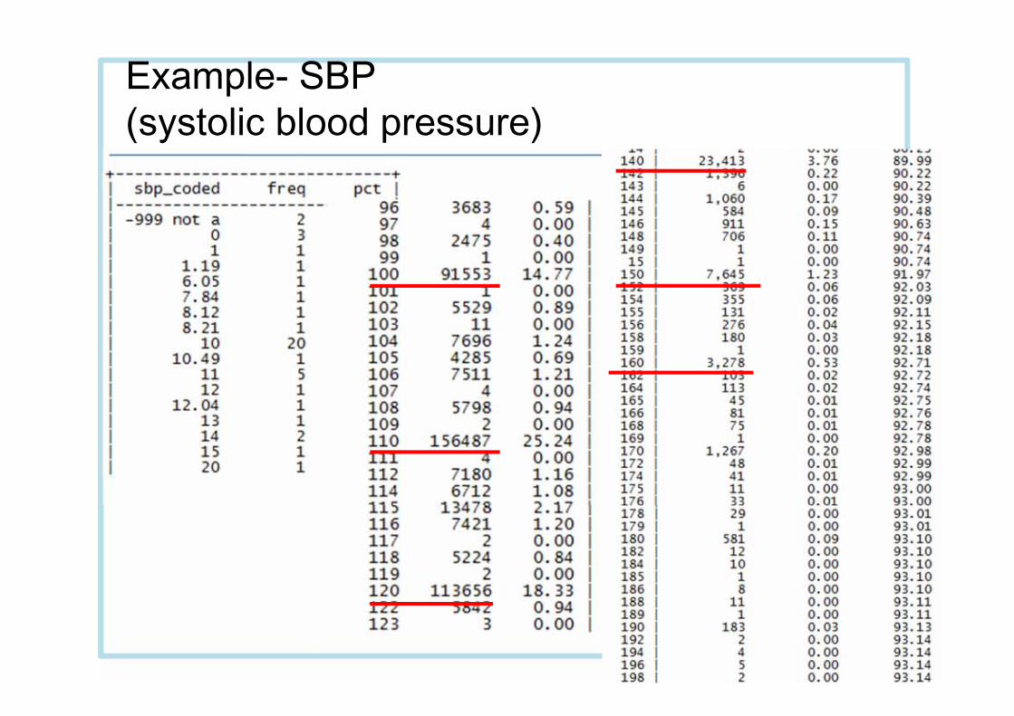
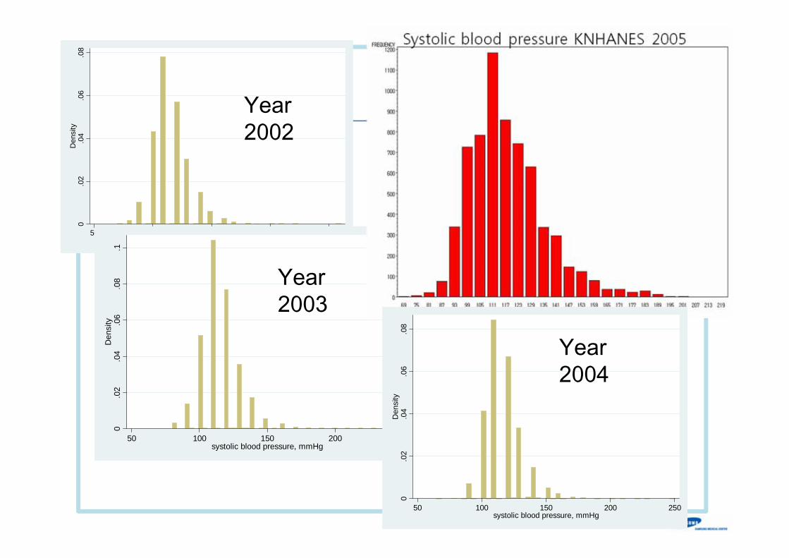
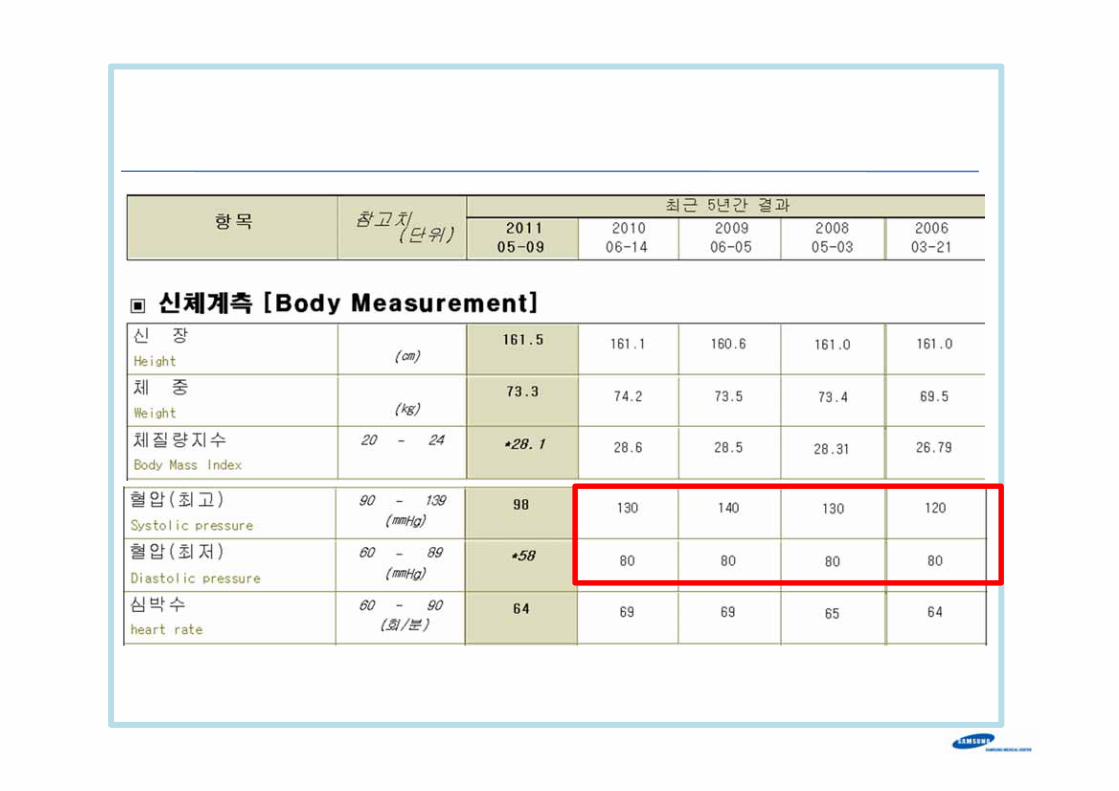
Example- SBP (systolic blood pressure)

0.0

2.0

4.0

6.0

8D

ensi

ty

50 100 150 200 250systolic blood pressure, mmHg

0.0

2.0

4.0

6.0

8.1

Den

sity

50 100 150 200 250systolic blood pressure, mmHg

Year 2002

Year 2003

0.0

2.0

4.0

6.0

8D

ensi

ty

50 100 150 200 250systolic blood pressure, mmHg

Year 2004

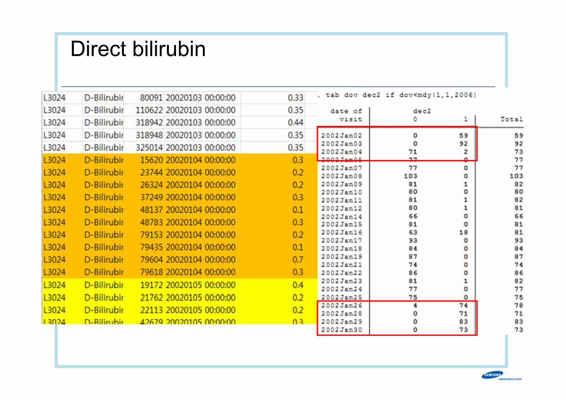
Direct bilirubin

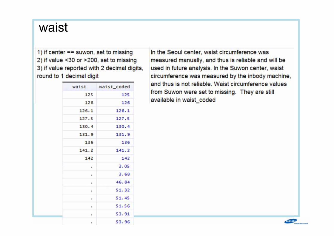
waist

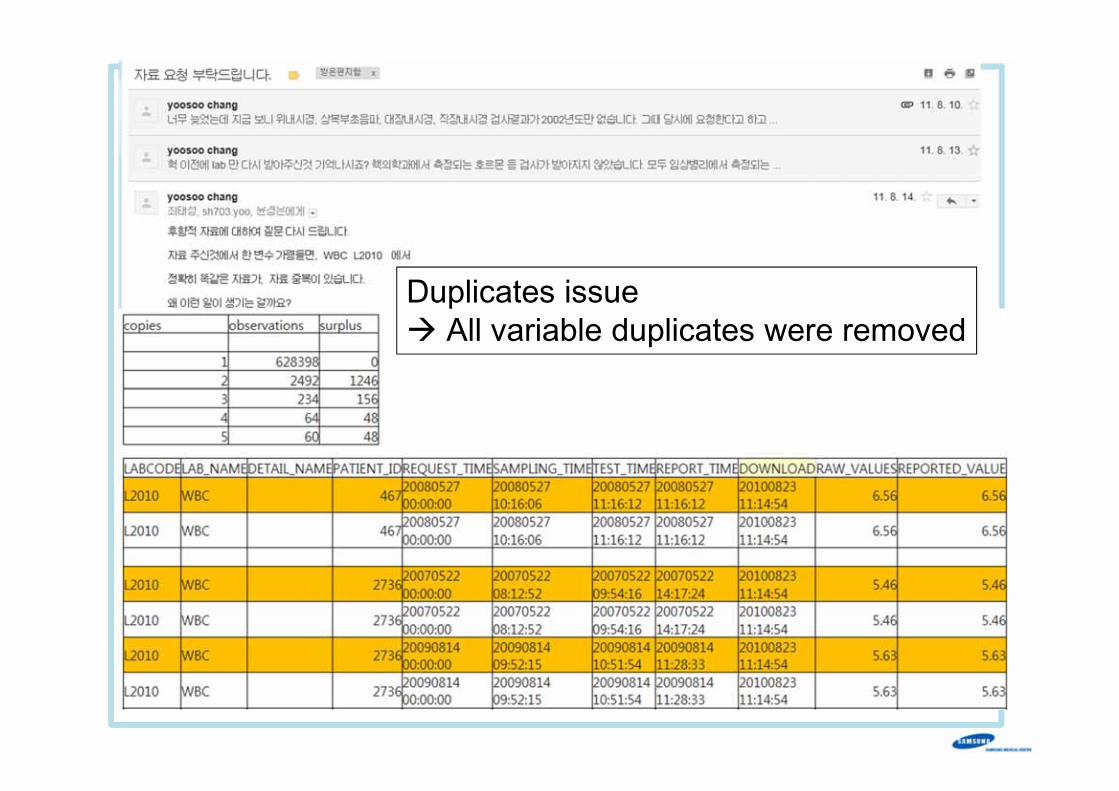
Duplicates issueAll variable duplicates were removed

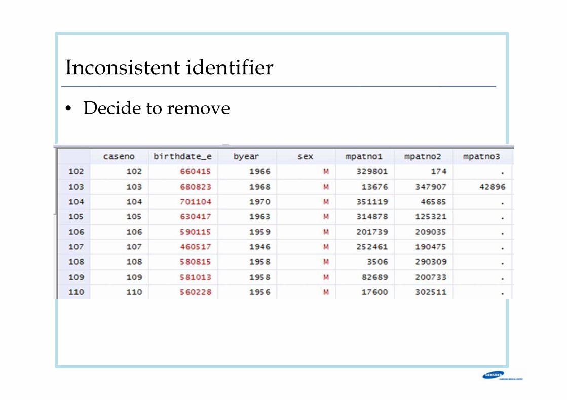
Inconsistent identifier

• Decide to remove

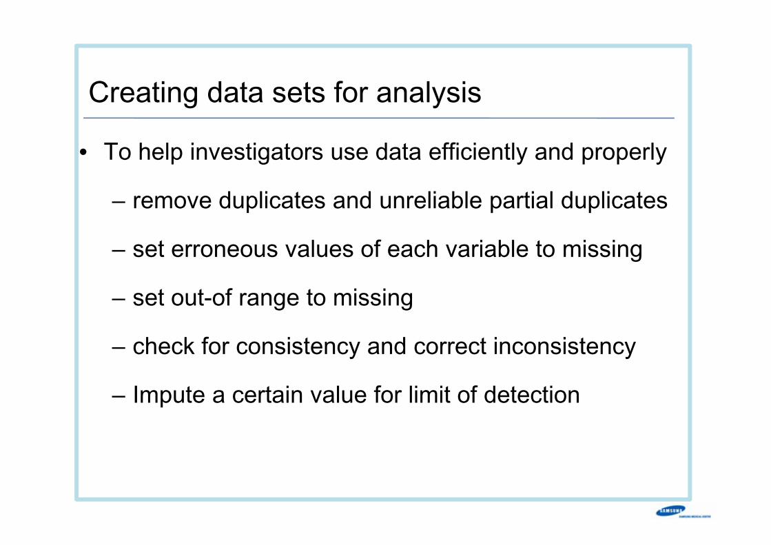
Creating data sets for analysis

• To help investigators use data efficiently and properly

– remove duplicates and unreliable partial duplicates

– set erroneous values of each variable to missing

– set out-of range to missing

– check for consistency and correct inconsistency

– Impute a certain value for limit of detection

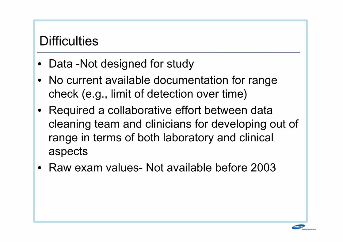
Difficulties• Data -Not designed for study• No current available documentation for range

check (e.g., limit of detection over time)• Required a collaborative effort between data

cleaning team and clinicians for developing out of range in terms of both laboratory and clinical aspects

• Raw exam values- Not available before 2003

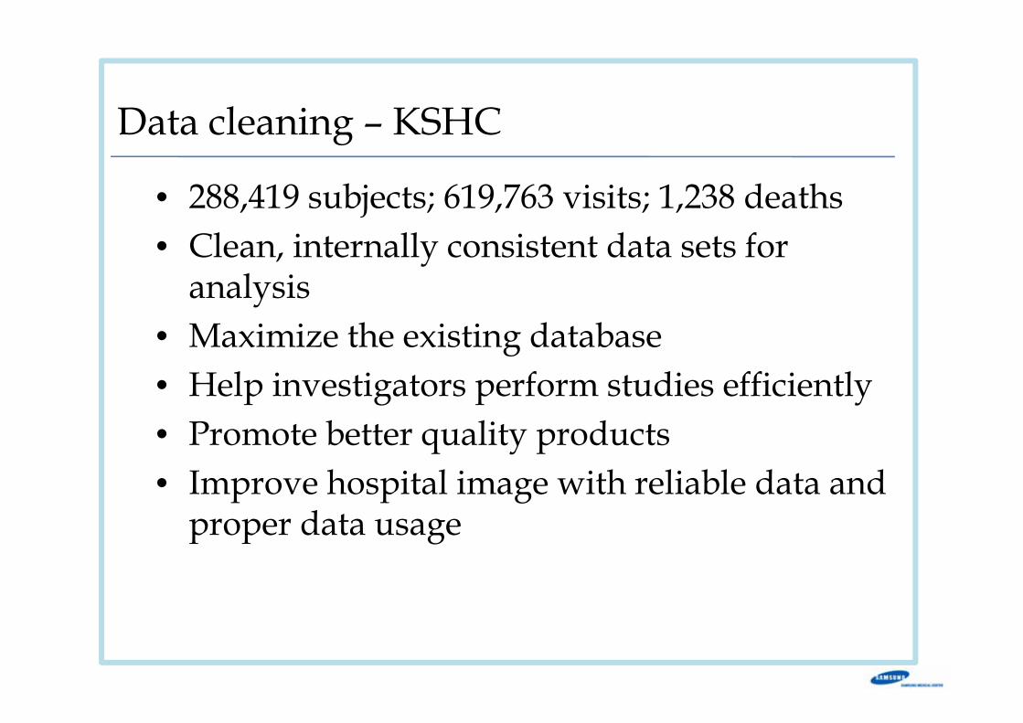
Data cleaning – KSHC

• 288,419 subjects; 619,763 visits; 1,238 deaths • Clean, internally consistent data sets for

analysis• Maximize the existing database• Help investigators perform studies efficiently• Promote better quality products• Improve hospital image with reliable data and

proper data usage

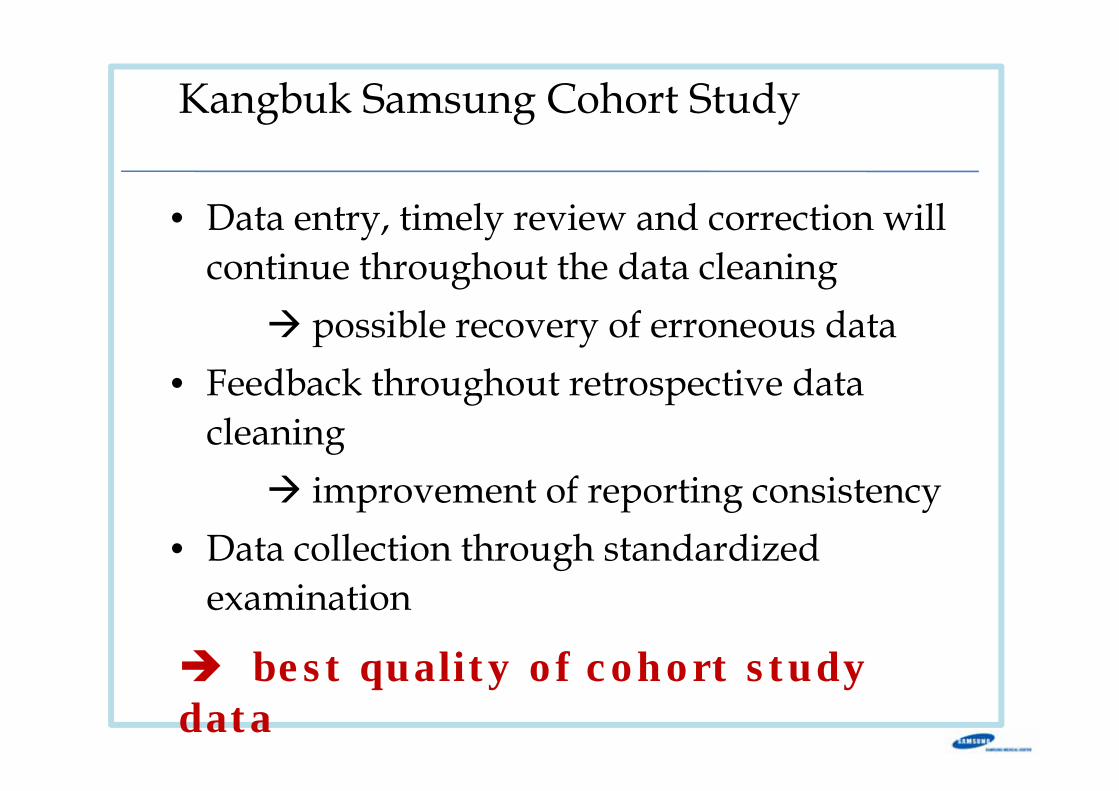
Kangbuk Samsung Cohort Study

• Data entry, timely review and correction will continue throughout the data cleaning

possible recovery of erroneous data• Feedback throughout retrospective data

cleaningimprovement of reporting consistency

• Data collection through standardized examination

best quality of cohort study data

Exploratory Data Analysis

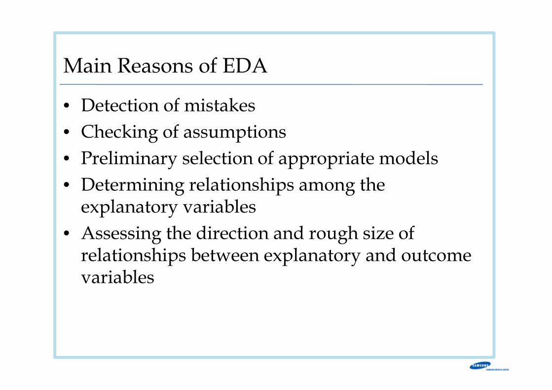
Main Reasons of EDA

• Detection of mistakes• Checking of assumptions• Preliminary selection of appropriate models• Determining relationships among the

explanatory variables• Assessing the direction and rough size of

relationships between explanatory and outcome variables

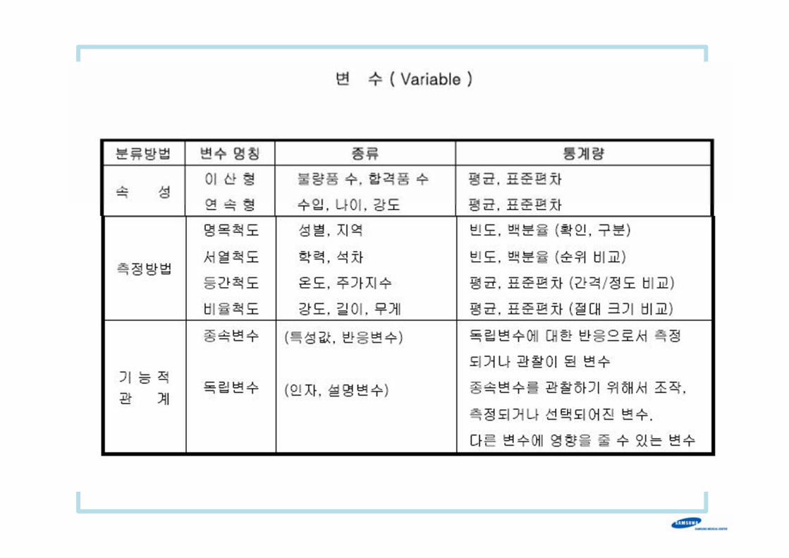
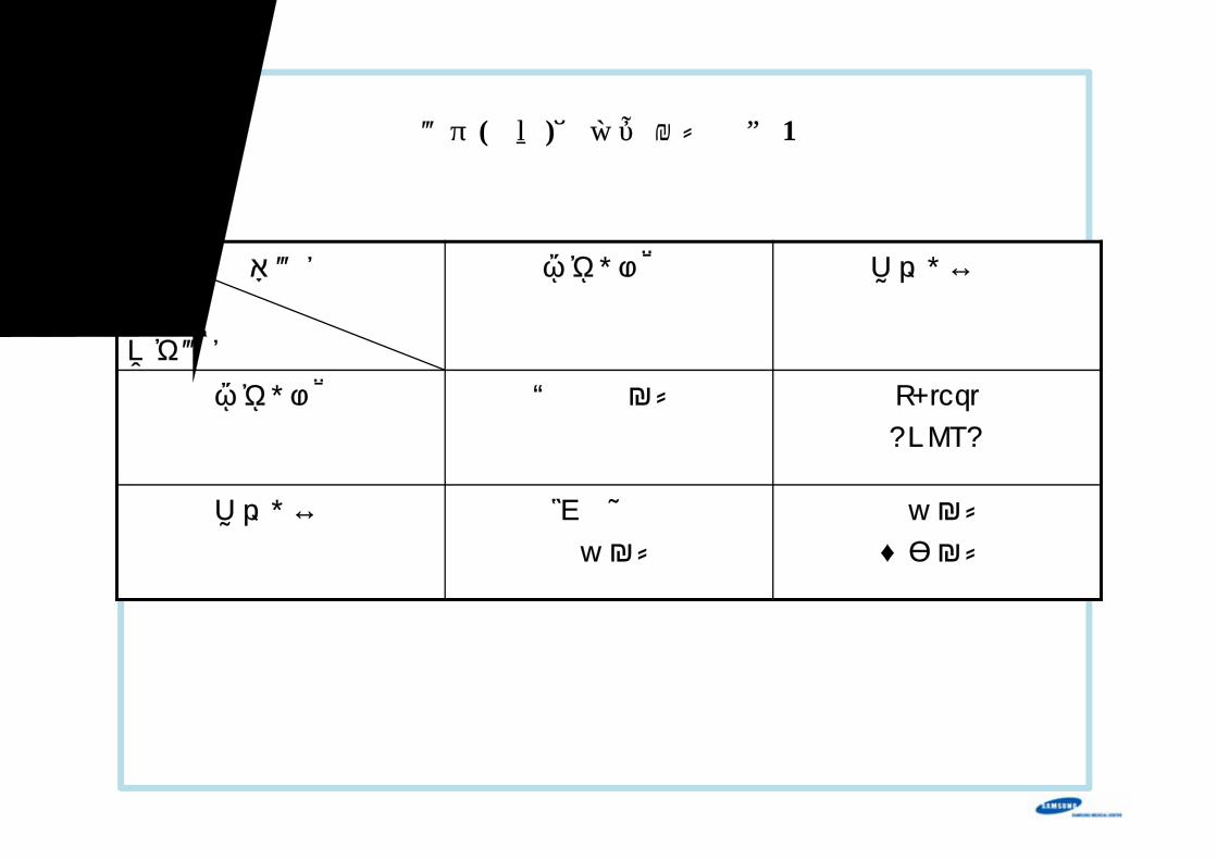
변수(척도)에따른분석방법 1

종속변수

독립변수

명목, 서열 등간, 비율

명목, 서열 범주형 분석 T-test

ANOVA

등간, 비율 로지스틱

회귀분석

회귀분석

상관분석

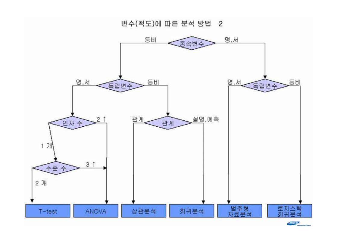
통계분석

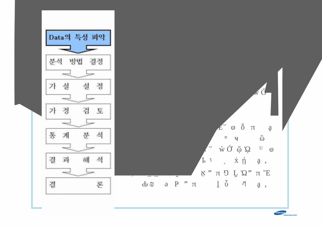
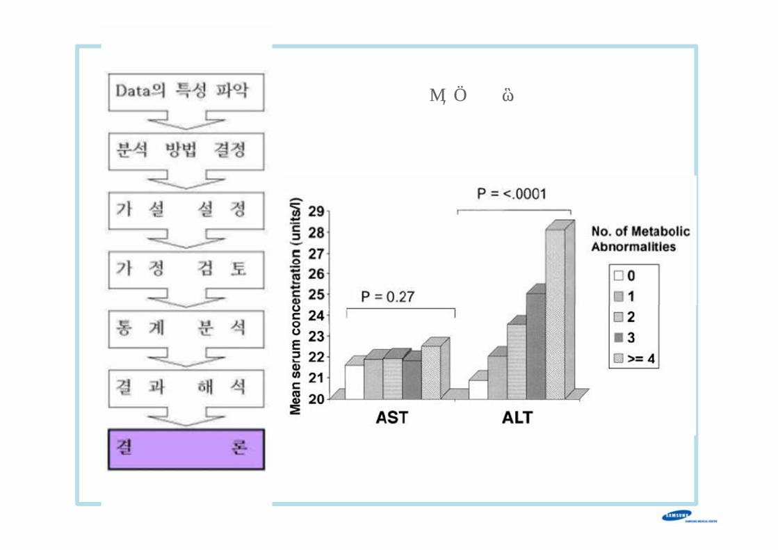
• 분석절차• Data의특성파악• 분석방법• 가설설정• 가정검토• 분석• 결과정리및해석

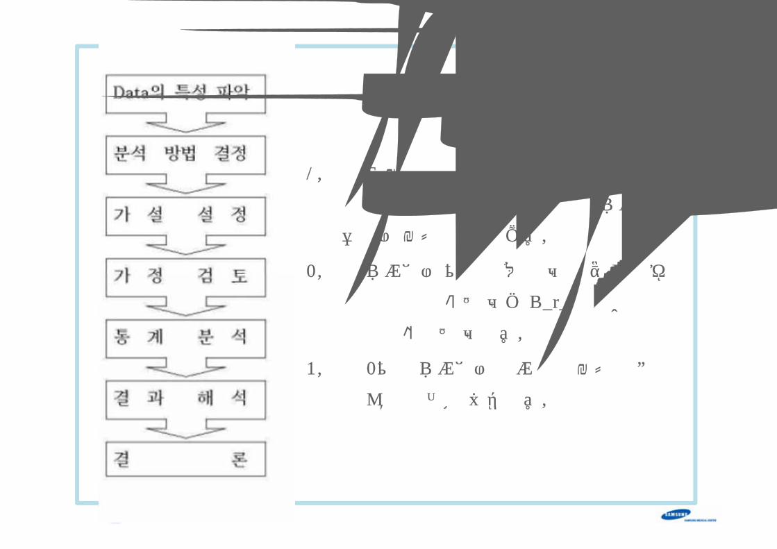
통 계 분 석 절 차

1. 통계 분석 절차는 연구 선정 및 연구 목

적을 명확히 결정한 후 다음의 7단계를

거쳐서 분석을 하게 된다.

2. 이 단계에서 가정 중요한 것은 연구의 목

적을 정확히 아는 것과 Data의 특성을 정

확히 파악하는 것이다.

3. 이 2가지 단계에서 통계적인 분석 방법

이 결정이 나기 때문이다.

Data의 특성 파악 1

1. 통계 분석 방법은 연구를 선정하고, Data

를 수집하는 단계에서 이미 결정이 난다.

앞서 본 내용대로 Data의 특성에 따라 분

석할 수 있는 통계적 기법은 거의 정해져

있기 때문이다.

2. 그러므로 Data 수집단계에서 될 수 있다

면 변수를 등비로 수집하는 것이 유리하

다. 등비척도는 경우에 따라 명목이나 서

열 척도로 변환이 가능하기 때문이다.

3. Data의 특성은 종속변수와 독립변수로

구분하고 각 변수의 척도를 파악한다.

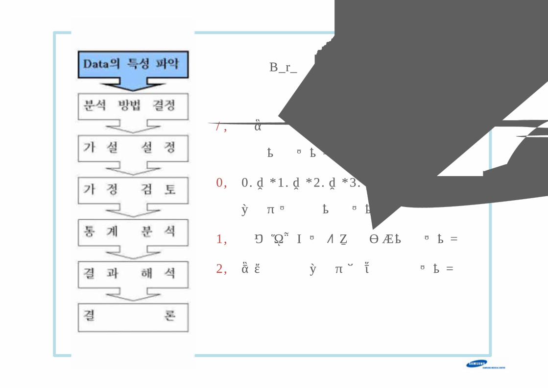
Data의 특성 파악 예제

1. 흡연 유무에 따라 체질량지수 (BMI)는

차이가 있는가?

2. 20대, 30대, 40대, 50대의 연령에 체질

량지수는 차이가 있는가?

3. 키와 몸무게는 어떠한 관계가 있는가?

4. 연령이 체질량지수에 영향을 주는가?

Data의 특성 파악 예제

1. T-test: 두 group 간 평균 비교

2. ANOVA: 두 group 이상 평균 비교

3. 상관분석: 두 변수 사이의 관계

4. 회귀분석: 독립변수에 따라 종속변수의

변화를 설명 예측

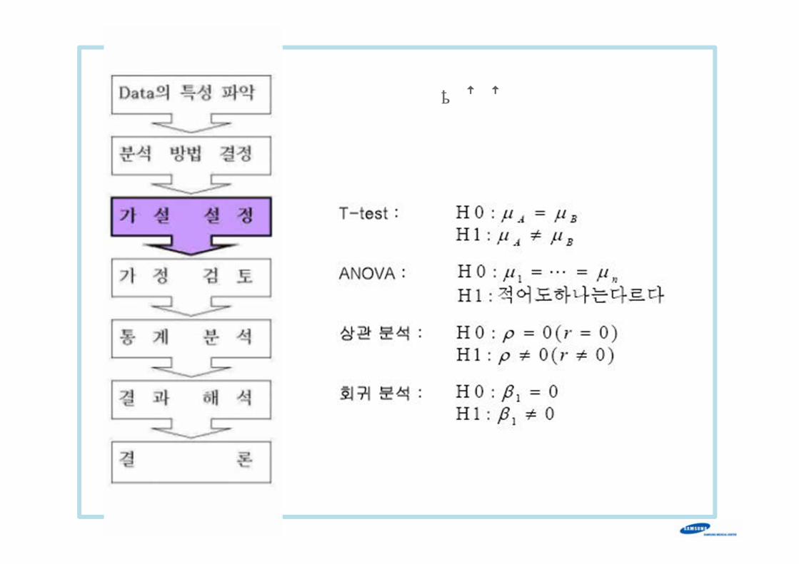
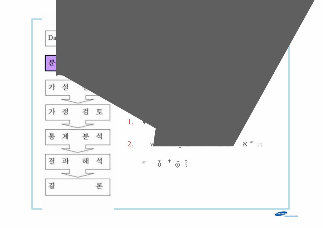
가 설 설 정

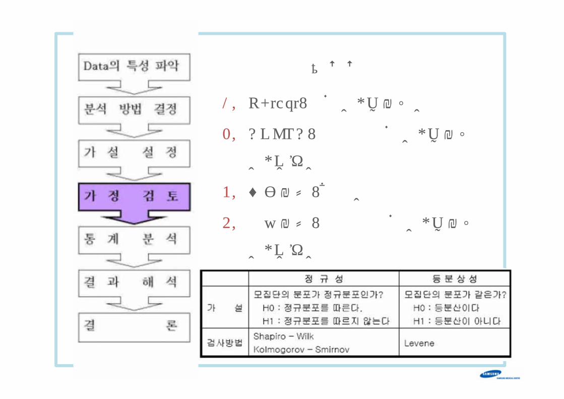
가 설 설 정

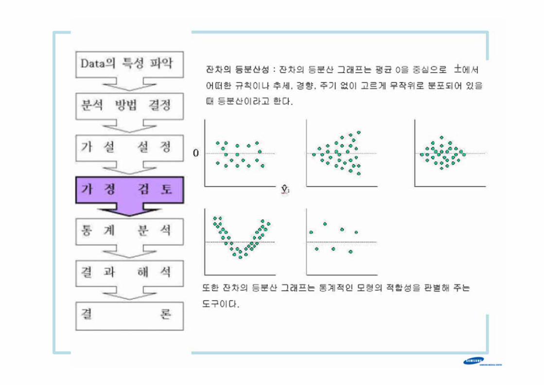
1. T-test: 정규성, 등분산성

2. ANOVA: 잔차의 정규성, 등분산

성, 독립성

3. 상관분석: 선형성

4. 회귀분석: 잔차의 정규성, 등분산

성, 독립성

통 계 분 석

1. 앞의 단계들에서 결정된 최종적인 분석

방법을 STATA에서 통계적인 분석을 실

시한다.

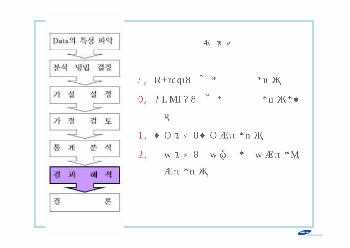
통 계 분 석

1. T-test: 평균, 표준편차, p 값

2. ANOVA: 평균, 표준편차, p 값, 사

후검정

3. 상관분석: 상관계수, p 값

4. 회귀분석: 회귀모형, 회귀계수, 결

정계수, p 값

결 과 정 리

Univariate Analysis

Measures of central location

MeanMedianGeometric mean

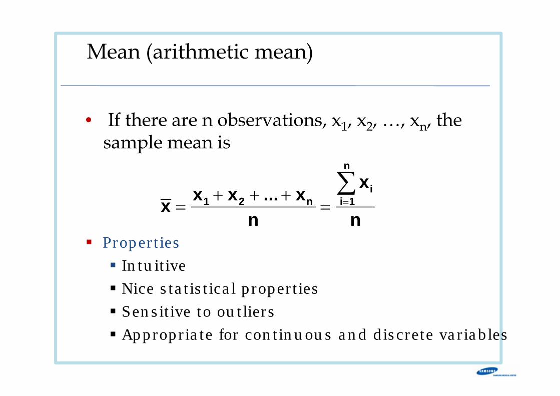
Mean (arithmetic mean)

• If there are n observations, x1, x2, …, xn, the sample mean is

n

x

nx...xxx

n

1ii

n21∑==

+++=

PropertiesIntuitiveNice statistical propertiesSensitive to outliersAppropriate for continuous and discrete variables

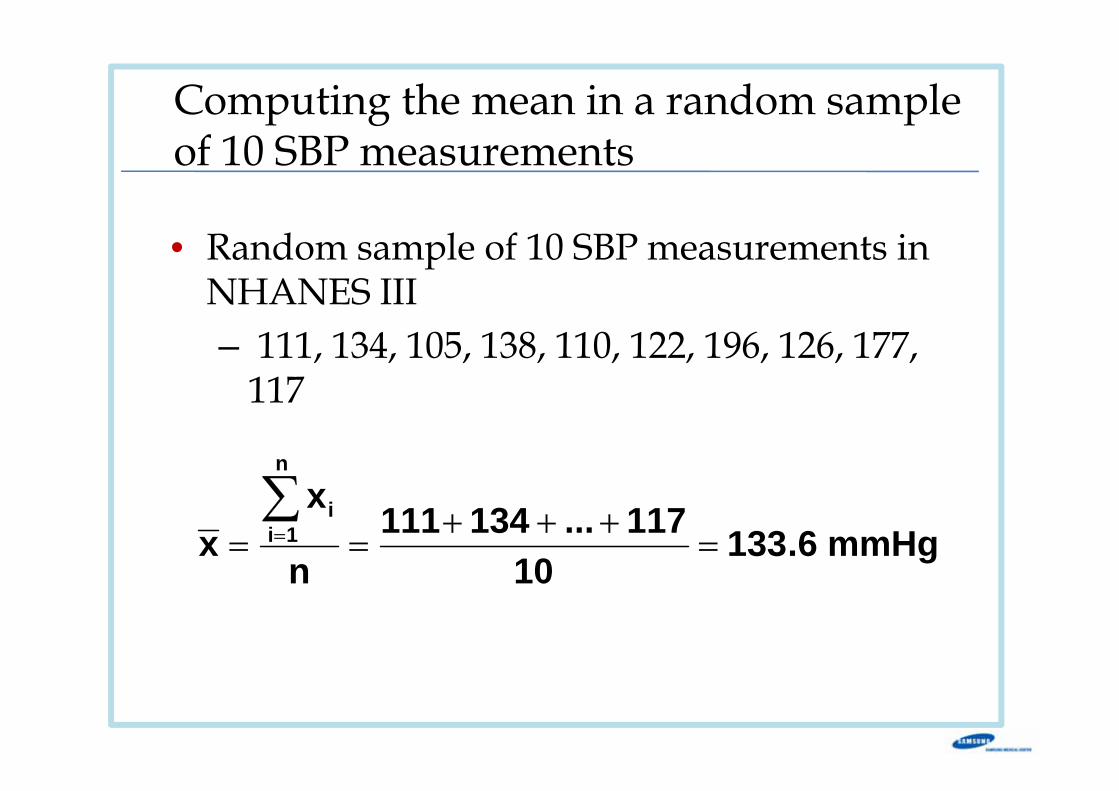
Computing the mean in a random sample of 10 SBP measurements

• Random sample of 10 SBP measurements in NHANES III– 111, 134, 105, 138, 110, 122, 196, 126, 177,

117

mmHg6.13310

117...134111n

xx

n

1ii

=+++

==∑=

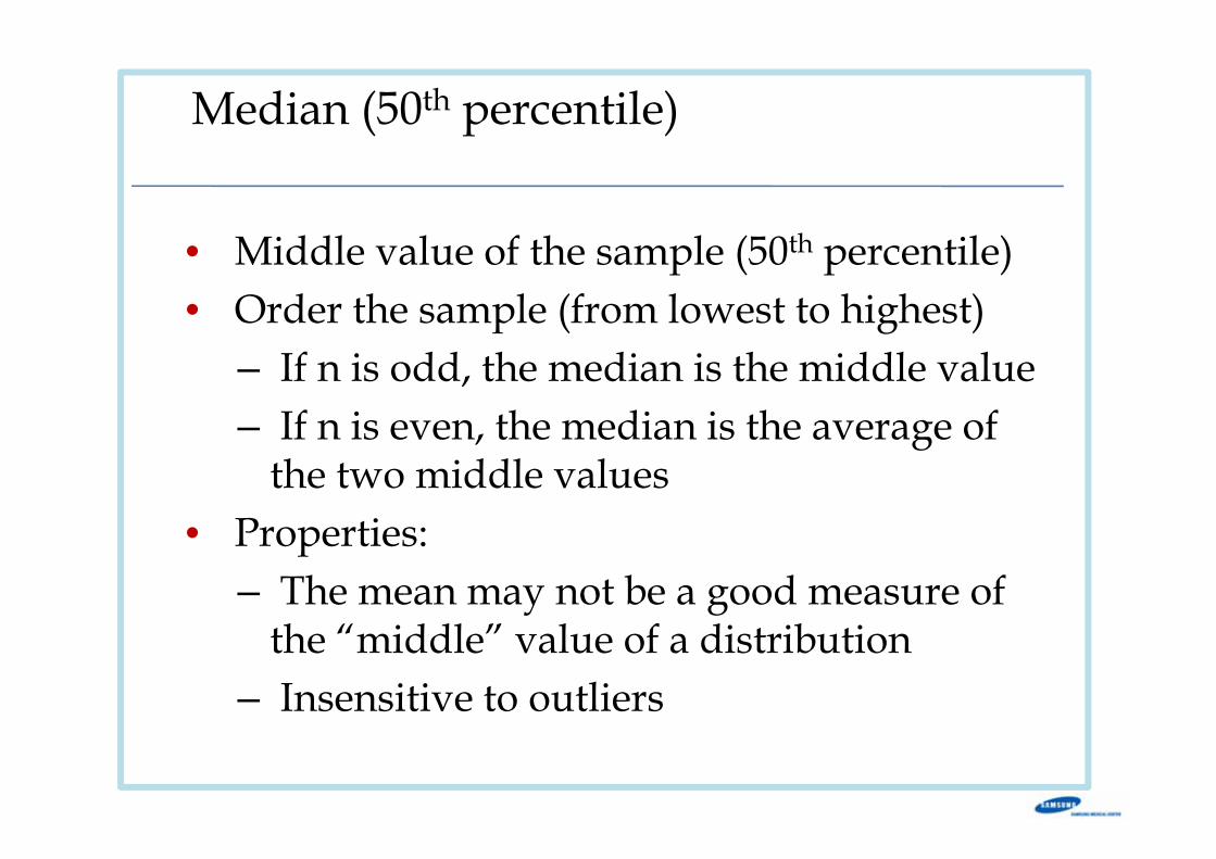
Median (50th percentile)

• Middle value of the sample (50th percentile)• Order the sample (from lowest to highest)

– If n is odd, the median is the middle value– If n is even, the median is the average of

the two middle values• Properties:

– The mean may not be a good measure of the “middle” value of a distribution

– Insensitive to outliers

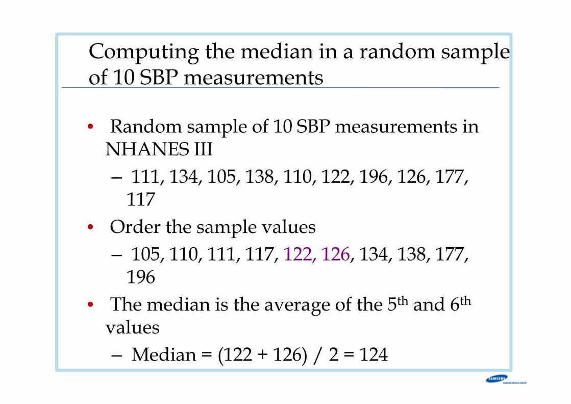
Computing the median in a random sample of 10 SBP measurements

• Random sample of 10 SBP measurements in NHANES III– 111, 134, 105, 138, 110, 122, 196, 126, 177,

117• Order the sample values

– 105, 110, 111, 117, 122, 126, 134, 138, 177, 196

• The median is the average of the 5th and 6th

values– Median = (122 + 126) / 2 = 124

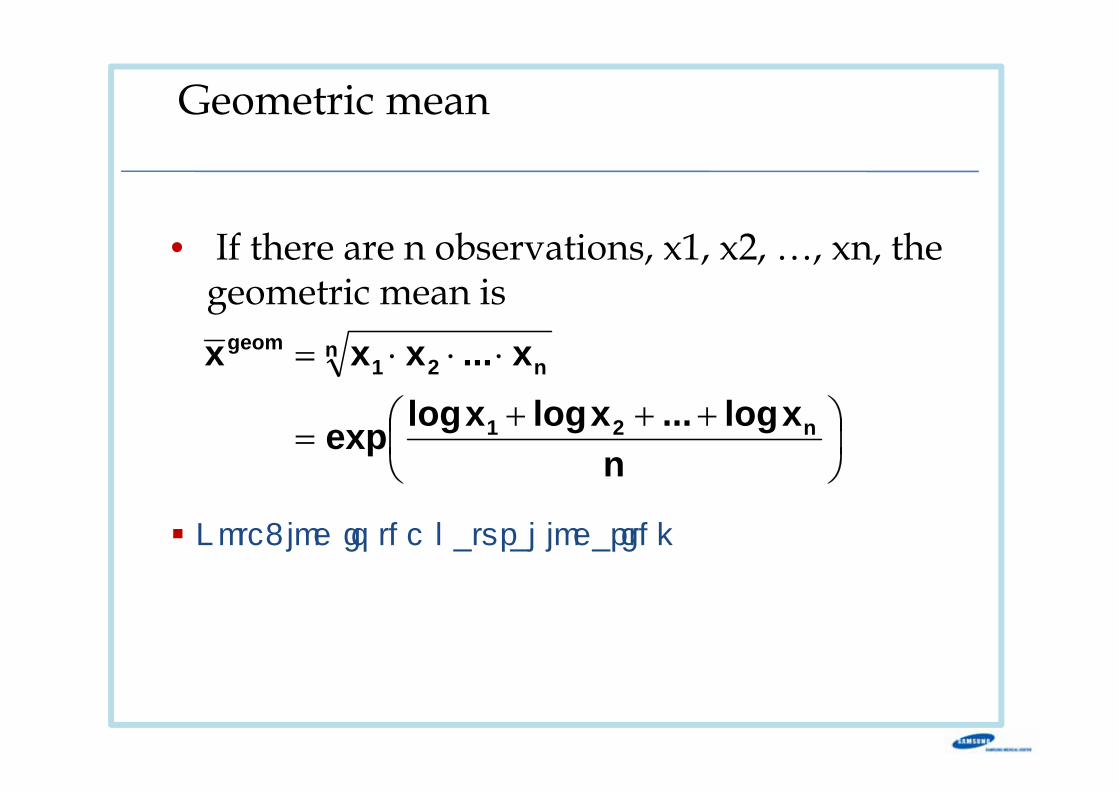
Geometric mean

• If there are n observations, x1, x2, …, xn, the geometric mean is

⎟⎠⎞

⎜⎝⎛ +++

=

⋅⋅⋅=

nxlog...xlogxlogexp

x...xxx

n21

nn21

geom

Note: log is the natural logarithm

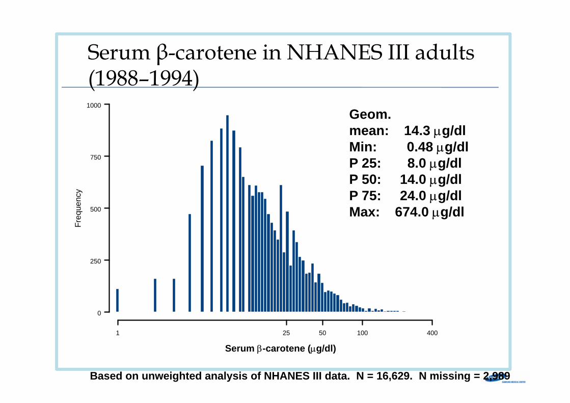
Freq

uenc

y

1 25 50 100 400

0

250

500

750

1000

Serum β-carotene in NHANES III adults (1988–1994)

Geom. mean: 14.3 µg/dlMin: 0.48 µg/dlP 25: 8.0 µg/dlP 50: 14.0 µg/dlP 75: 24.0 µg/dlMax: 674.0 µg/dl

Based on unweighted analysis of NHANES III data. N = 16,629. N missing = 2,989

Serum β-carotene (µg/dl)

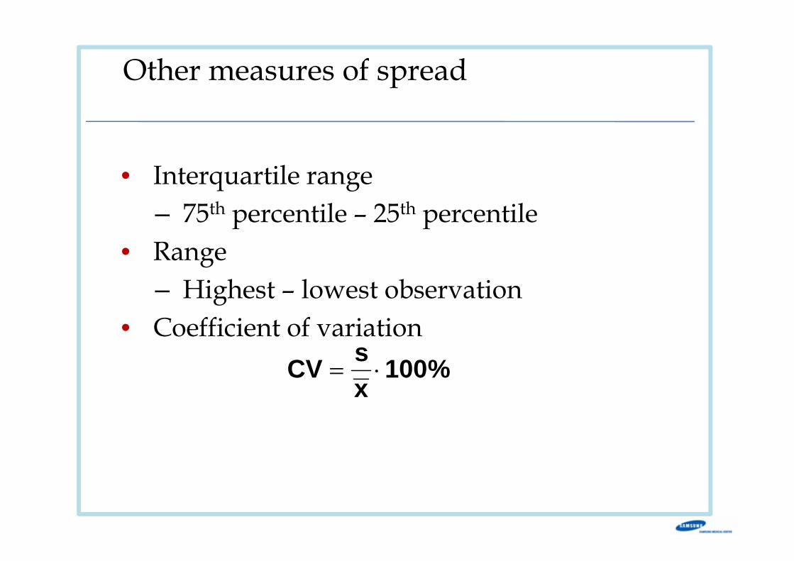
Measures of spread

Standard deviationInterquartile rangeRangeCoefficient of variation

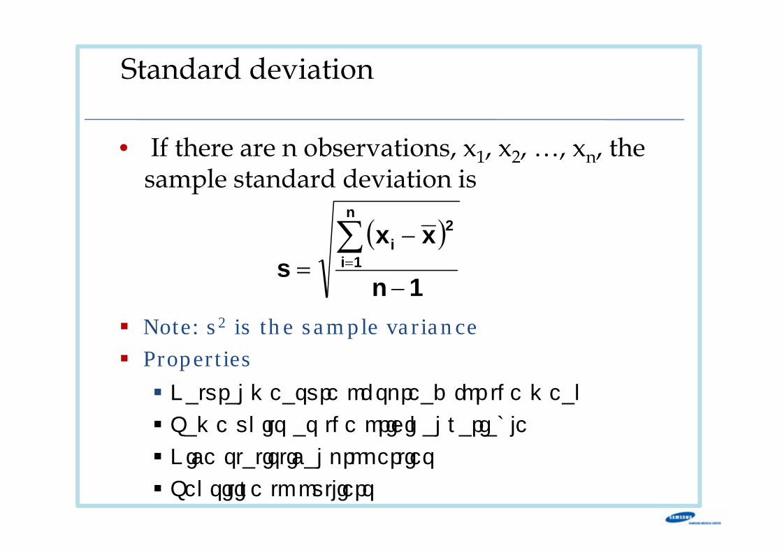
Standard deviation

• If there are n observations, x1, x2, …, xn, the sample standard deviation is

( )

1n

xxs

n

1i

2i

−

−=∑=

Note: s2 is the sample variancePropertiesNatural measure of spread for the mean

Same units as the original variable

Nice statistical properties

Sensitive to outliers

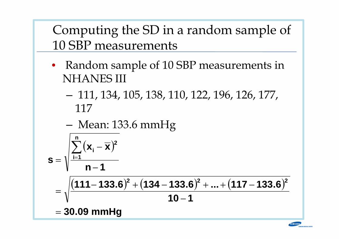
Computing the SD in a random sample of 10 SBP measurements• Random sample of 10 SBP measurements in

NHANES III– 111, 134, 105, 138, 110, 122, 196, 126, 177,

117– Mean: 133.6 mmHg

( )

( ) ( ) ( )

mmHg09.30110

6.133117...6.1331346.133111

1n

xxs

222

n

1i

2i

=−

−++−+−=

−

−=∑=

Other measures of spread

• Interquartile range– 75th percentile – 25th percentile

• Range– Highest – lowest observation

• Coefficient of variation%100

xsCV ⋅=

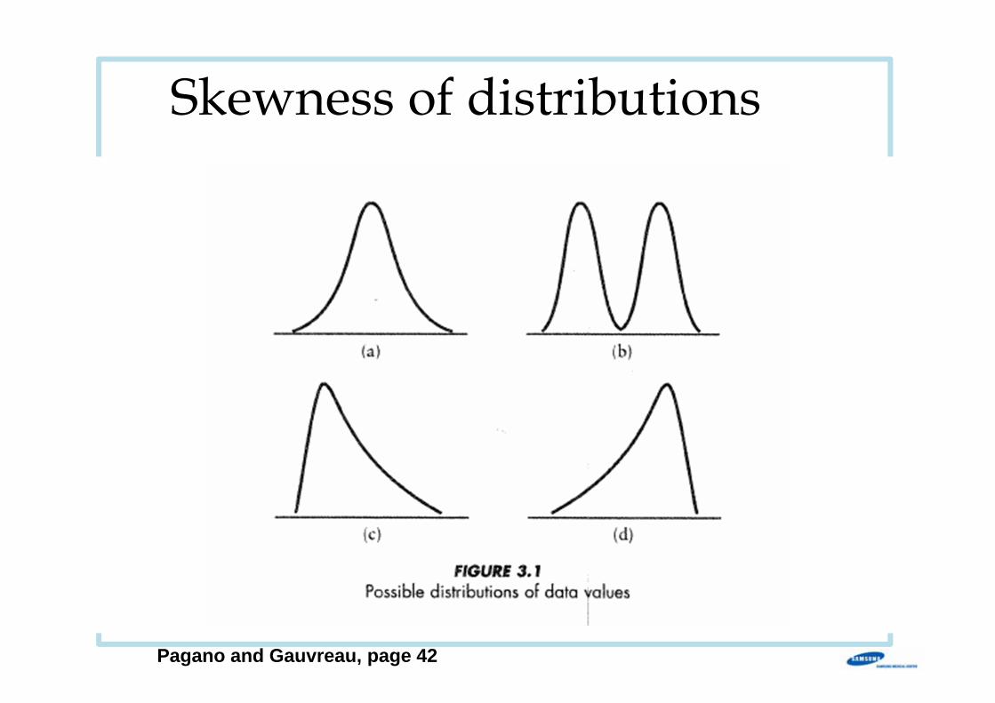
Skewness of distributions

Pagano and Gauvreau, page 42

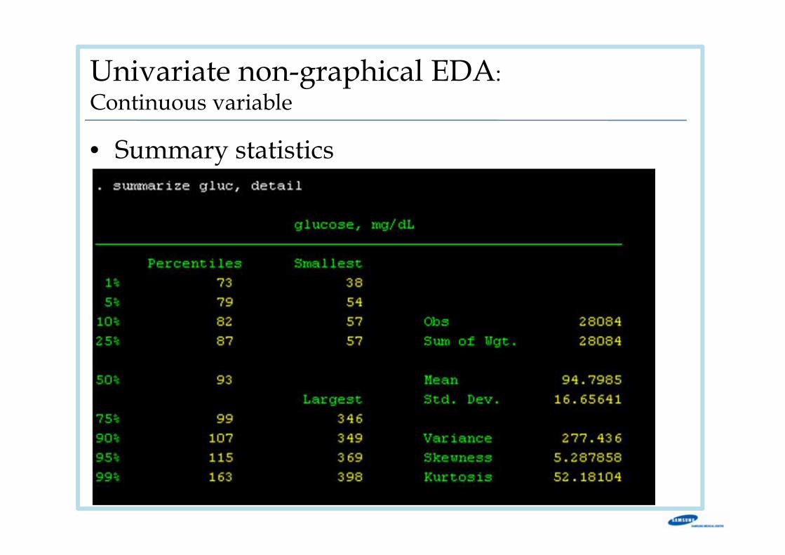
Univariate non-graphical EDA: Continuous variable

• Summary statistics

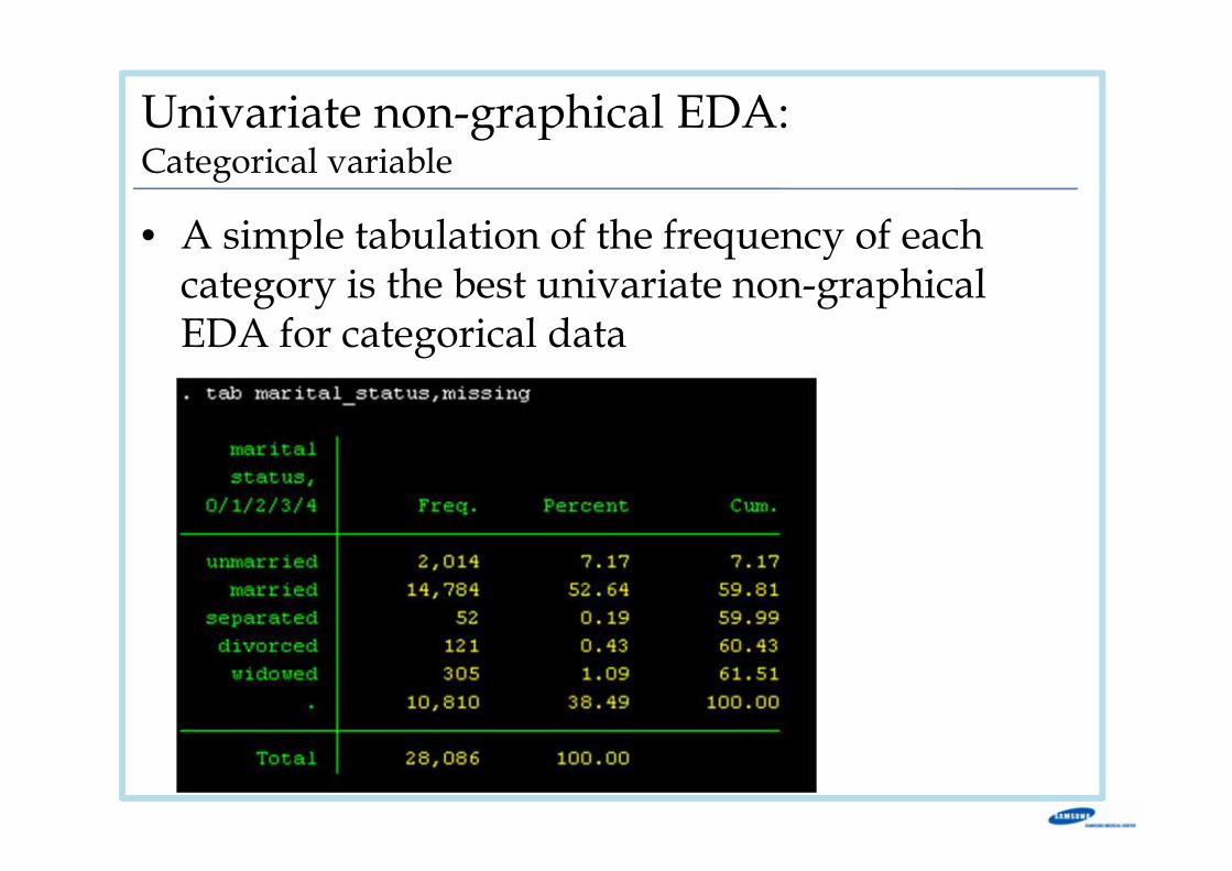
Univariate non-graphical EDA: Categorical variable

• A simple tabulation of the frequency of each category is the best univariate non-graphical EDA for categorical data

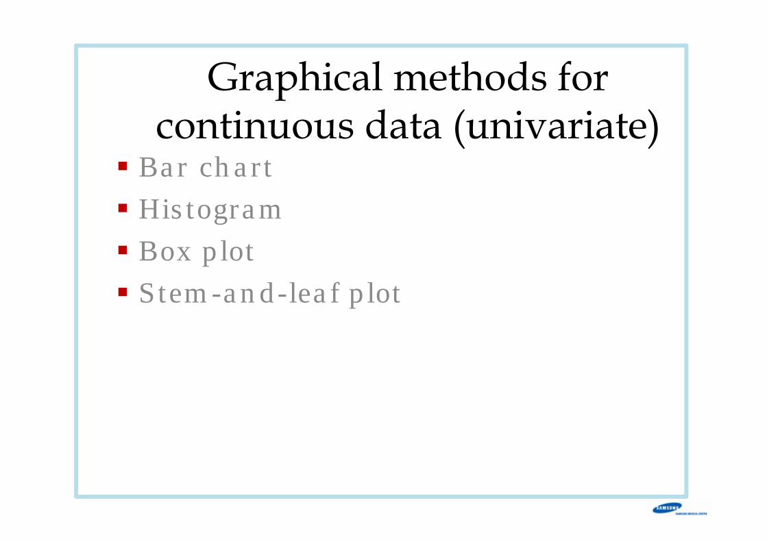
Graphical methods for continuous data (univariate)

Bar chartHistogramBox plotStem-and-leaf plot

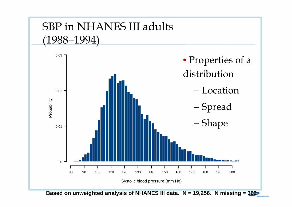
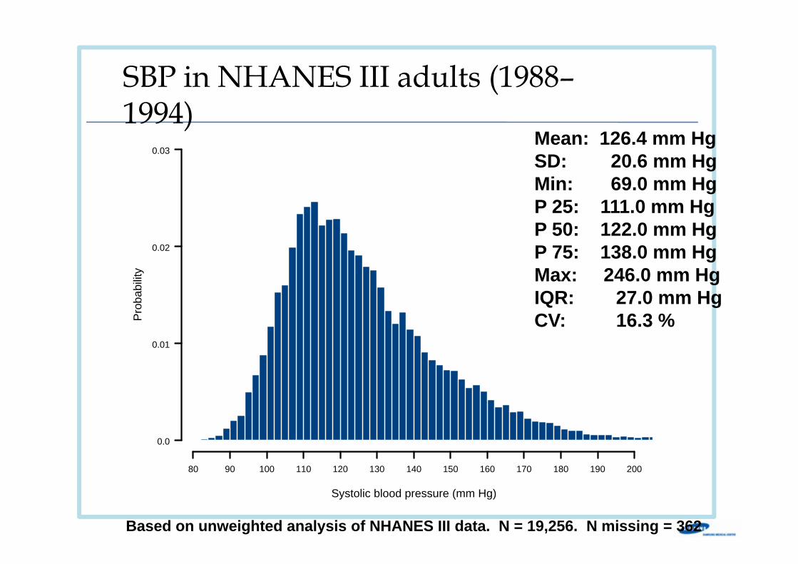
Systolic blood pressure (mm Hg)

Pro

babi

lity

80 90 100 110 120 130 140 150 160 170 180 190 200

0.0

0.01

0.02

0.03

SBP in NHANES III adults (1988–1994)

Based on unweighted analysis of NHANES III data. N = 19,256. N missing = 362

• Properties of a distribution

– Location– Spread– Shape

Systolic blood pressure (mm Hg)

Pro

babi

lity

80 90 100 110 120 130 140 150 160 170 180 190 200

0.0

0.01

0.02

0.03

SBP in NHANES III adults (1988–1994)

Mean: 126.4 mm HgSD: 20.6 mm HgMin: 69.0 mm HgP 25: 111.0 mm HgP 50: 122.0 mm HgP 75: 138.0 mm HgMax: 246.0 mm HgIQR: 27.0 mm HgCV: 16.3 %

Based on unweighted analysis of NHANES III data. N = 19,256. N missing = 362

Histogram

• The key with a histogram is to use a sufficient number of intervals to define the shape of the distribution clearly and not lose much information.

• A rough rule of thumb is to choose the number of bins to be about 1+3.3log10(n) where no is the sample size.

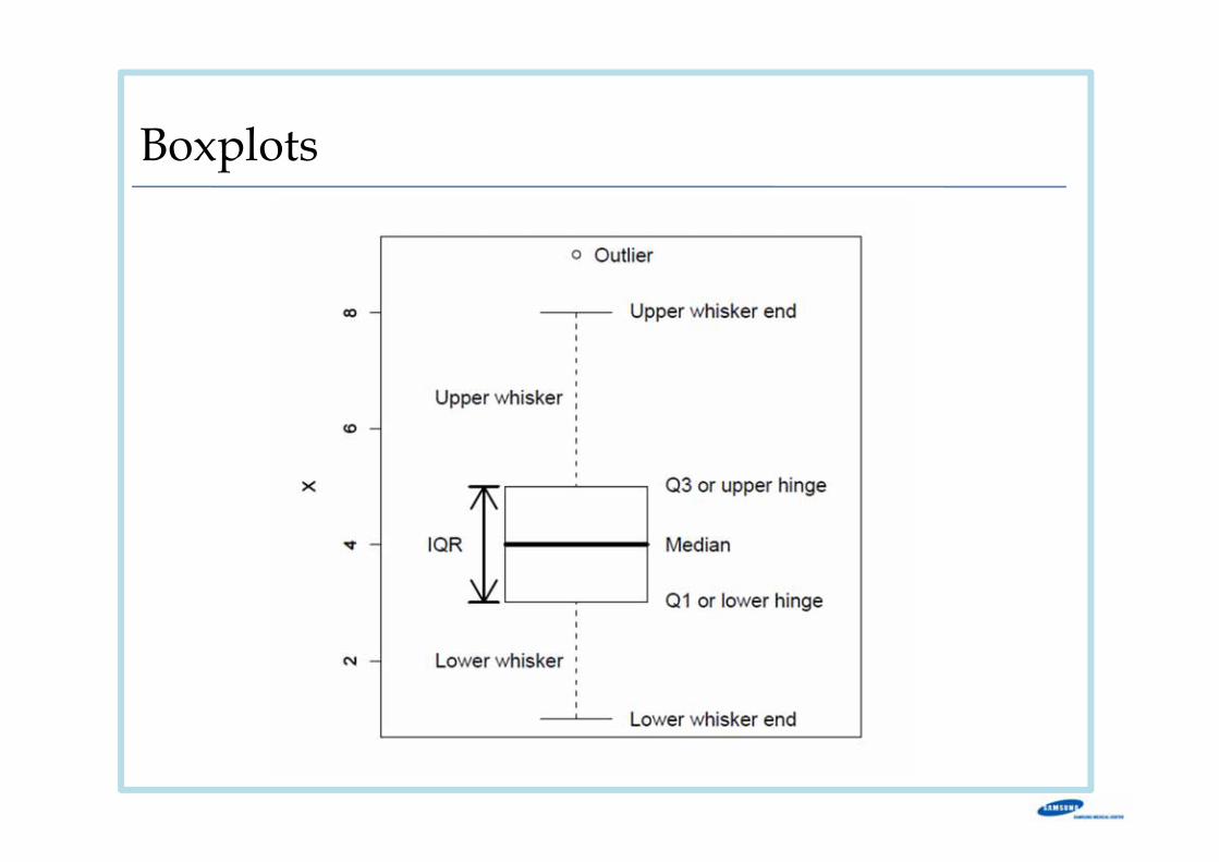
Boxplots

Boxplot

• Location, as measured by the median• Spead, as measured by the height of the box (this

is called the interquartile range for IQR)• Range of the observations• Presence of outliers• Some information about shape

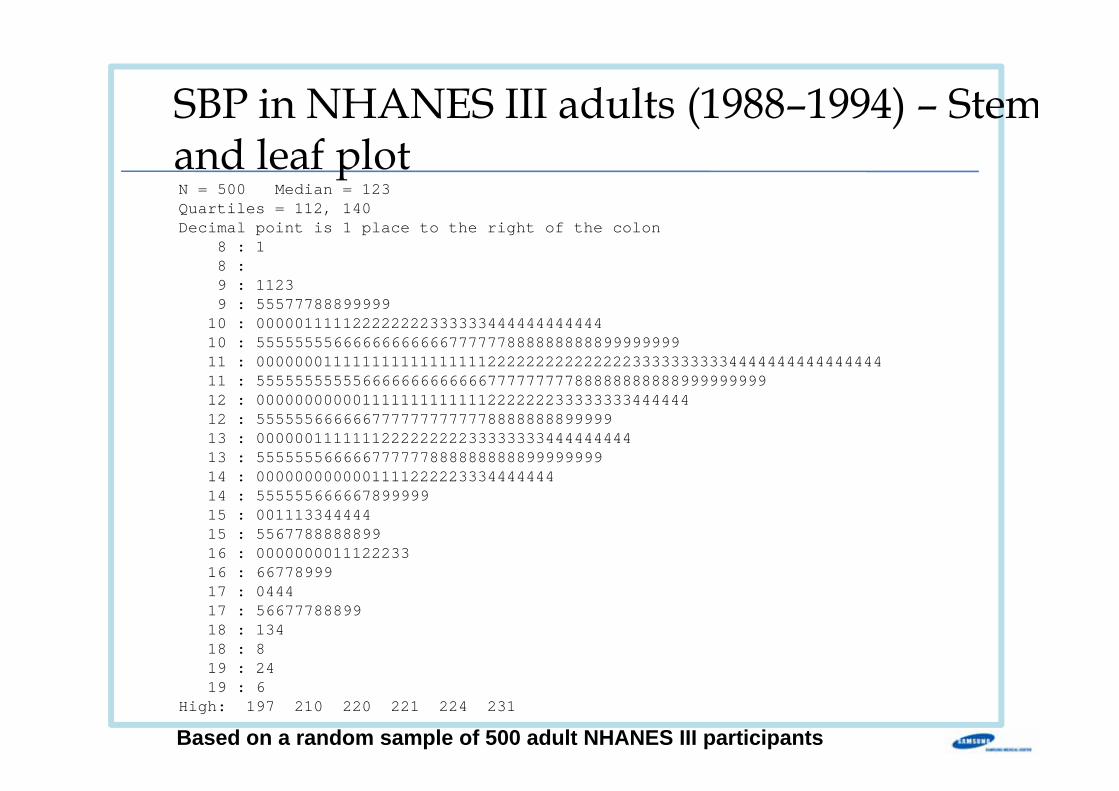
SBP in NHANES III adults (1988–1994) – Stemand leaf plot

Based on a random sample of 500 adult NHANES III participants

N = 500 Median = 123Quartiles = 112, 140Decimal point is 1 place to the right of the colon

8 : 18 :9 : 11239 : 55577788899999

10 : 00000111112222222233333344444444444410 : 5555555566666666666677777788888888889999999911 : 0000000111111111111111112222222222222223333333333444444444444444411 : 5555555555566666666666667777777778888888888899999999912 : 00000000000111111111111122222223333333344444412 : 555555666666777777777777888888889999913 : 00000011111112222222223333333344444444413 : 55555556666677777788888888889999999914 : 000000000000111122222333444444414 : 55555566666789999915 : 00111334444415 : 556778888889916 : 000000001112223316 : 6677899917 : 044417 : 5667778889918 : 13418 : 819 : 2419 : 6

High: 197 210 220 221 224 231

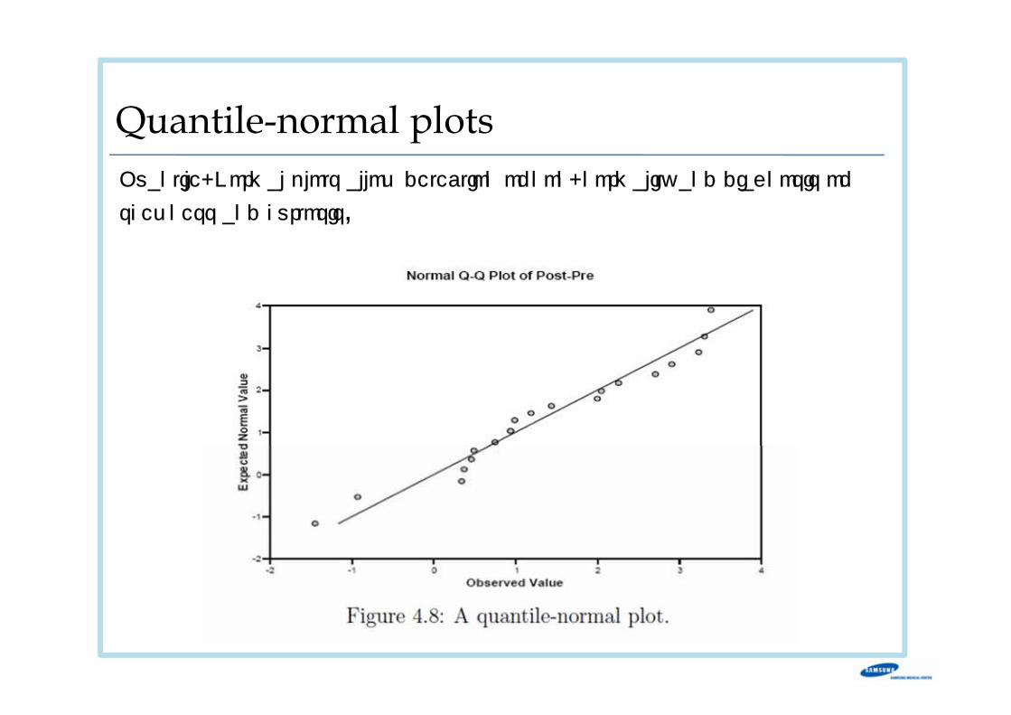
Quantile-normal plotsQuantile-Normal plots allow detection of non-normality and diagnosis of

skewness and kurtosis.

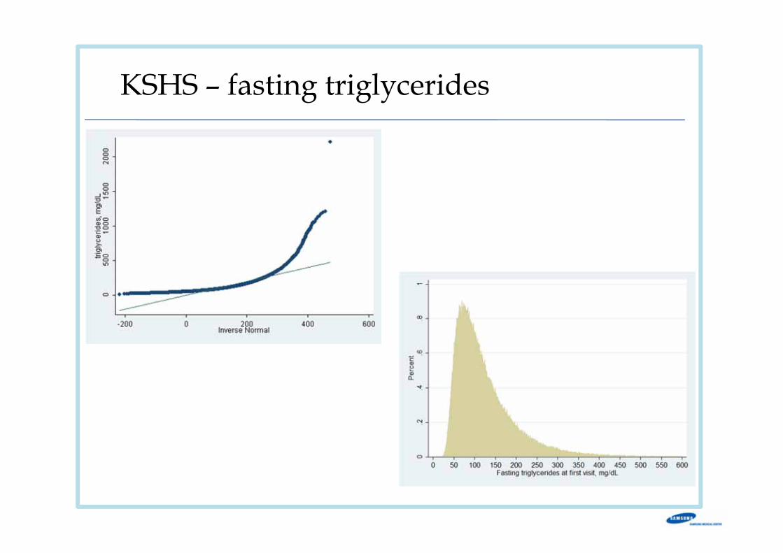
KSHS – fasting triglycerides

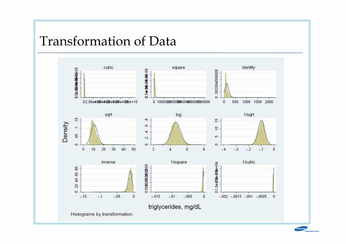
Transformation of Data

bivariate Analysis

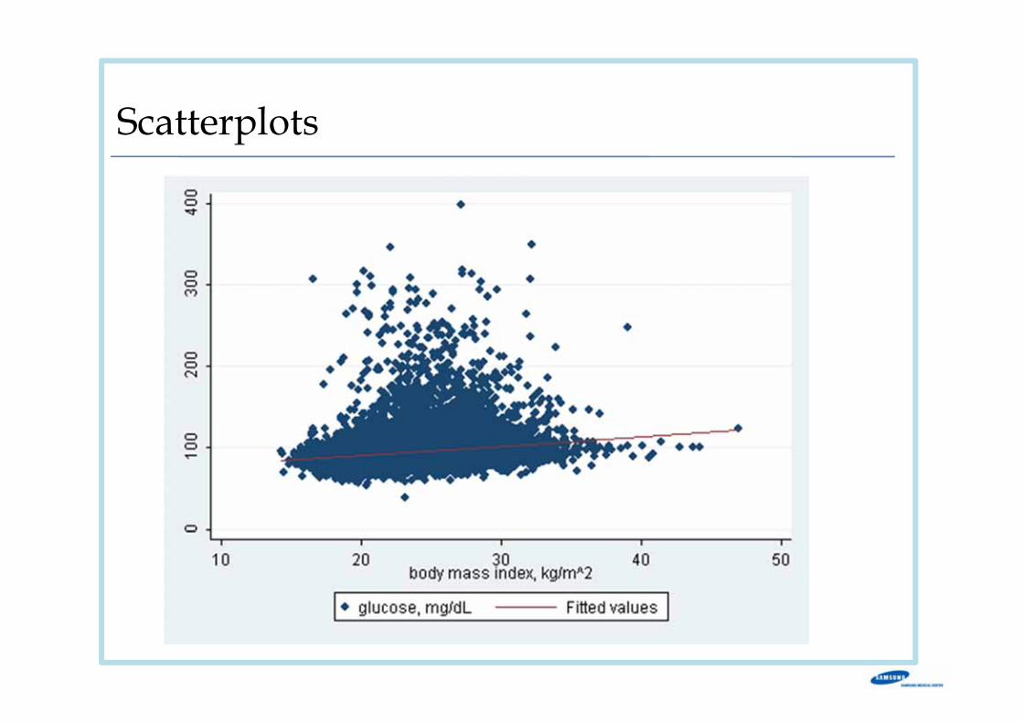
Scatterplots

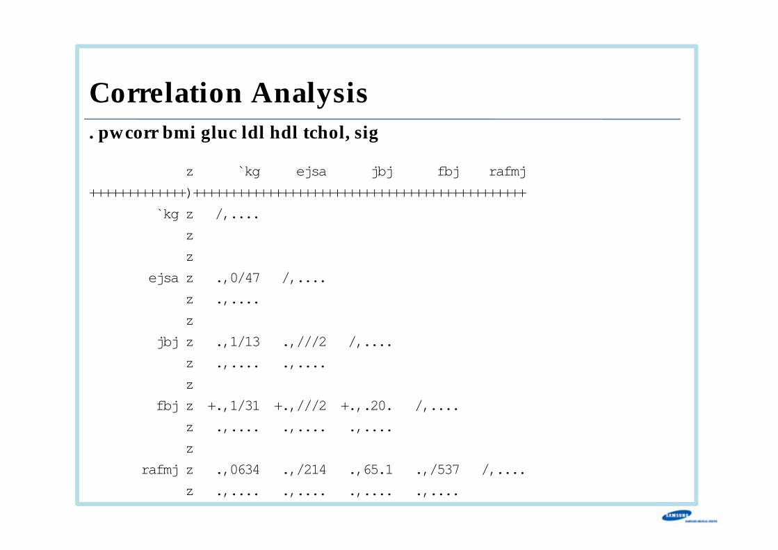
Correlation Analysis. pwcorr bmi gluc ldl hdl tchol, sig

| bmi gluc ldl hdl tchol

-------------+---------------------------------------------

bmi | 1.0000

|

|

gluc | 0.2169 1.0000

| 0.0000

|

ldl | 0.3135 0.1114 1.0000

| 0.0000 0.0000

|

hdl | -0.3153 -0.1114 -0.0420 1.0000

| 0.0000 0.0000 0.0000

|

tchol | 0.2856 0.1436 0.8703 0.1759 1.0000

| 0.0000 0.0000 0.0000 0.0000

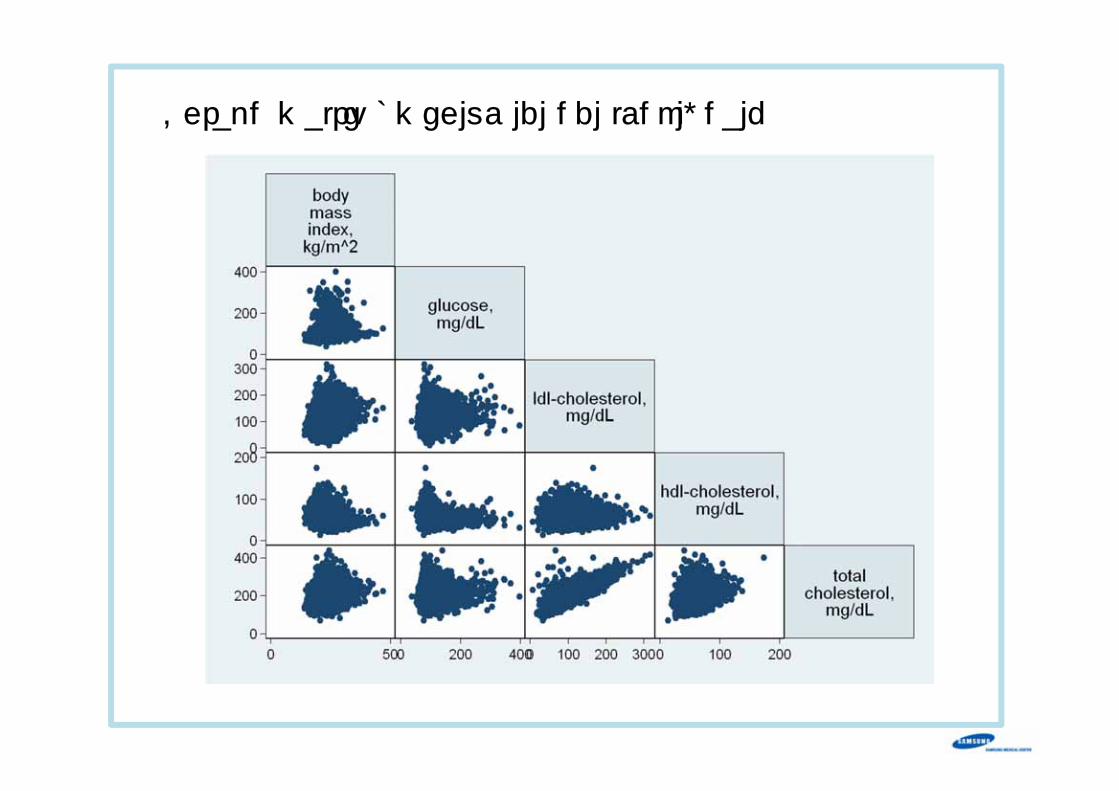
. graph matrix bmi gluc ldl hdl tchol, half

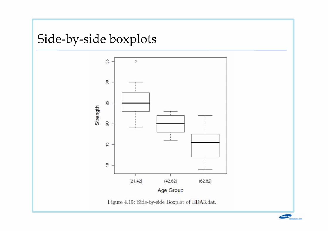
Side-by-side boxplots

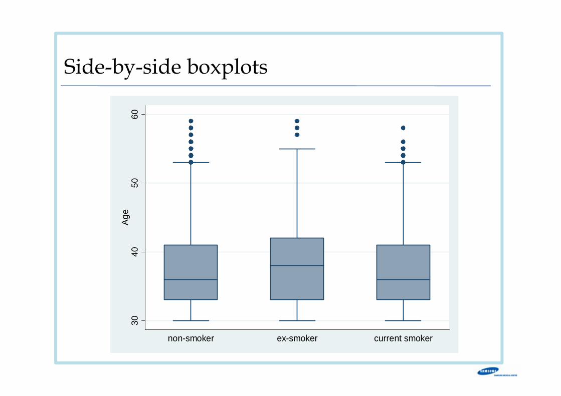
Side-by-side boxplots

3040

5060

Age

non-smoker ex-smoker current smoker

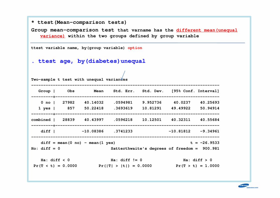
* ttest(Mean-comparison tests)Group mean-comparison test that varname has the different mean(unequal

variance) within the two groups defined by group variable

ttest variable name, by(group variable) option

. ttest age, by(diabetes)unequal

Two-sample t test with unequal variances------------------------------------------------------------------------------

Group | Obs Mean Std. Err. Std. Dev. [95% Conf. Interval]---------+--------------------------------------------------------------------

0 no | 27982 40.14032 .0594981 9.952736 40.0237 40.256931 yes | 857 50.22418 .3693619 10.81291 49.49922 50.94914

---------+--------------------------------------------------------------------combined | 28839 40.43997 .0596218 10.12501 40.32311 40.55684---------+--------------------------------------------------------------------

diff | -10.08386 .3741233 -10.81812 -9.34961------------------------------------------------------------------------------

diff = mean(0 no) - mean(1 yes) t = -26.9533Ho: diff = 0 Satterthwaite's degrees of freedom = 900.981

Ha: diff < 0 Ha: diff != 0 Ha: diff > 0Pr(T < t) = 0.0000 Pr(|T| > |t|) = 0.0000 Pr(T > t) = 1.0000

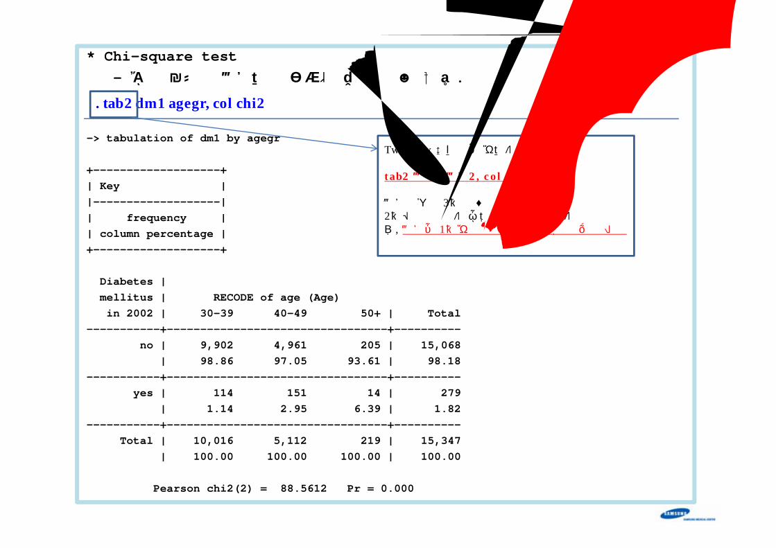
* Chi-square test– 먼저 분석할 변수들의 관계에 대하여 살펴본다.

. tab2 dm1 agegr, col chi2

-> tabulation of dm1 by agegr

+-------------------+| Key ||-------------------|| frequency || column percentage |+-------------------+

Diabetes |mellitus | RECODE of age (Age)in 2002 | 30-39 40-49 50+ | Total

-----------+---------------------------------+----------no | 9,902 4,961 205 | 15,068

| 98.86 97.05 93.61 | 98.18 -----------+---------------------------------+----------

yes | 114 151 14 | 279 | 1.14 2.95 6.39 | 1.82

-----------+---------------------------------+----------Total | 10,016 5,112 219 | 15,347

| 100.00 100.00 100.00 | 100.00

Pearson chi2(2) = 88.5612 Pr = 0.000

Two-way 빈도표를 만들어 주는 명령어 임

tab2 변수1 변수2, col chi2

변수이름이 3개 이상일 경우에는2개씩 짝을 지어 모든 빈도표를 만들어 줌단, 변수를 1개만 지정할 경우에는 실행되지 않음

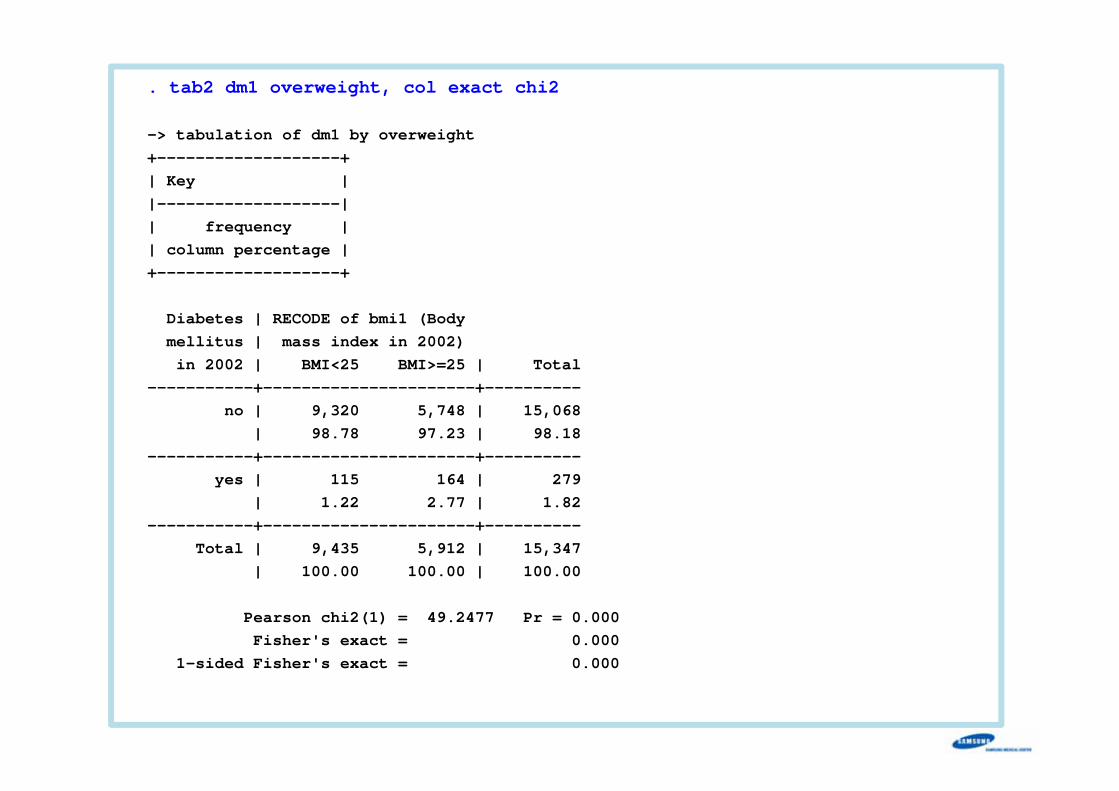
. tab2 dm1 overweight, col exact chi2

-> tabulation of dm1 by overweight +-------------------+| Key ||-------------------|| frequency || column percentage |+-------------------+

Diabetes | RECODE of bmi1 (Bodymellitus | mass index in 2002)in 2002 | BMI<25 BMI>=25 | Total

-----------+----------------------+----------no | 9,320 5,748 | 15,068

| 98.78 97.23 | 98.18 -----------+----------------------+----------

yes | 115 164 | 279 | 1.22 2.77 | 1.82

-----------+----------------------+----------Total | 9,435 5,912 | 15,347

| 100.00 100.00 | 100.00

Pearson chi2(1) = 49.2477 Pr = 0.000Fisher's exact = 0.000

1-sided Fisher's exact = 0.000

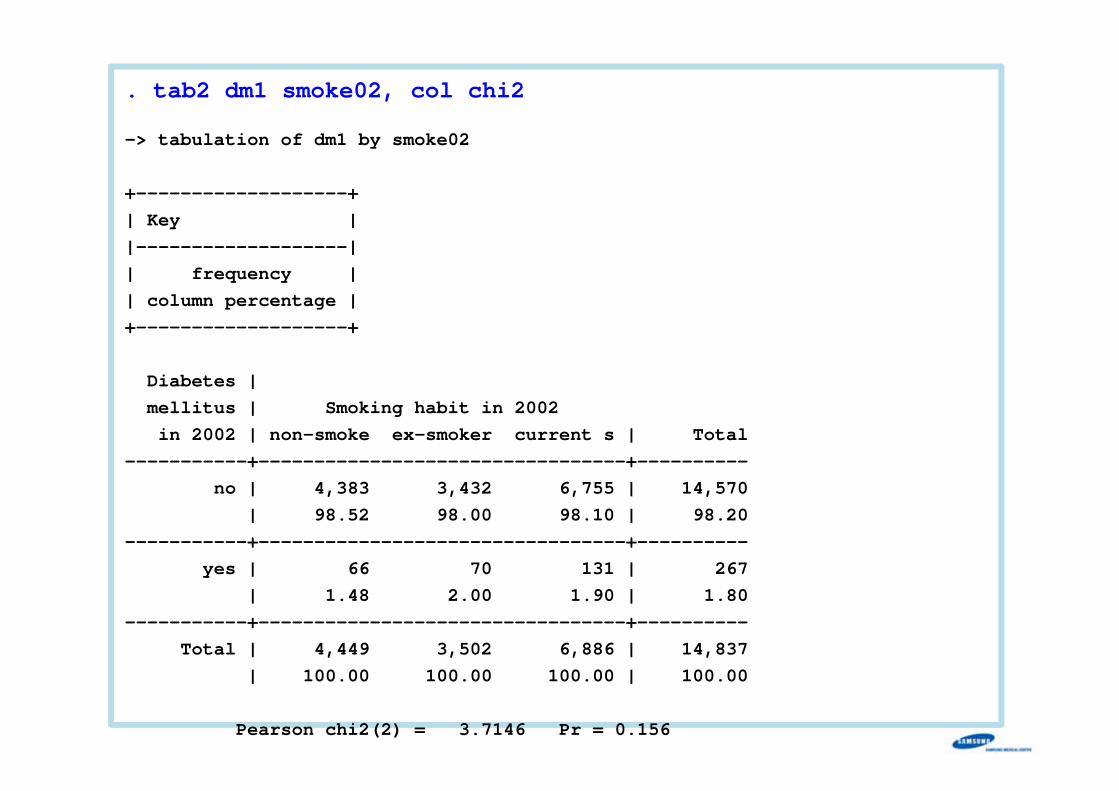
. tab2 dm1 smoke02, col chi2

-> tabulation of dm1 by smoke02

+-------------------+| Key ||-------------------|| frequency || column percentage |+-------------------+

Diabetes |mellitus | Smoking habit in 2002in 2002 | non-smoke ex-smoker current s | Total

-----------+---------------------------------+----------no | 4,383 3,432 6,755 | 14,570

| 98.52 98.00 98.10 | 98.20 -----------+---------------------------------+----------

yes | 66 70 131 | 267 | 1.48 2.00 1.90 | 1.80

-----------+---------------------------------+----------Total | 4,449 3,502 6,886 | 14,837

| 100.00 100.00 100.00 | 100.00

Pearson chi2(2) = 3.7146 Pr = 0.156