d3.2 prototype development of a fully integrated data ...d3... · d3.2 prototype development of a...
TRANSCRIPT

1
D3.2 Prototype development of a fully integrated data-driven simulator
DATA science for SIMulating the era of electric vehicles
www.datasim-fp7.eu
Project details
Project reference: 270833 Status: Execution Programme acronym: FP7-ICT (FET Open) Subprogramme area: ICT-2009.8.0 Future and Emerging Technologies Contract type: Collaborative project (generic)
Consortium details
Coordinator: 1. (UHasselt) Universiteit Hasselt
Partners: 2. (CNR) Consiglio Nazionale delle Ricerche 3. (BME) Budapesti Muszaki es Gazdasagtudomanyi Egyetem 4. (Fraunhofer) Fraunhofer-Gesellschaft zur Foerdering der Angewandten Forschung E.V 5. (UPM) Universidad Politecnica de Madrid 6. (VITO) Vlaamse Instelling voor Technologisch Onderzoek N.V. 7. (IIT) Technion – Israel Institute of Technology 8. (UPRC) University of Piraeus Research Center 9. (HU) University of Haifa
Contact details
Prof. dr. Davy Janssens Universiteit Hasselt– Transportation Research Institute (IMOB)
Function in DATA SIM: Person in charge of scientific and technical/technological aspects Address: Wetenschapspark 5 bus 6 | 3590 Diepenbeek | Belgium Tel.: +32 (0)11 26 91 28 Fax: +32 (0)11 26 91 99 E-mail: [email protected] URL: www.imob.uhasselt.be
Deliverable details
Work Package WP3 Deliverable: D3.2 Prototype development of a fully integrated data-driven simulator Dissemination level: PU Nature: R Contractual Date of Delivery: 31.08.2014 Actual Date of Delivery: 31.08.2014 Total number of pages: 40 (incl. 1 title page) Authors: Luk Knapen, Davy Janssens, Ansar Yasar
Abstract This document presents the work pursued in the third year of the project by the participants of WP3. The document presents the scientific results that constitute fundaments for the development of the new simulator.

Contents
1 General Information 31.1 Management Summary . . . . . . . . . . . . . . . . . . . . . . . . . . . . . . . . . . . . . . 31.2 List of DATASIM WP3 Related Publications for Year 3 . . . . . . . . . . . . . . . . . . . 4
2 Research Results 52.1 The Use of Big Data to feed Activity-Based Models . . . . . . . . . . . . . . . . . . . . . 5
2.1.1 iMOVE Diaries and GPS Traces . . . . . . . . . . . . . . . . . . . . . . . . . . . . 52.1.1.1 The iMOVE Data Analysis in the DATASIM Project . . . . . . . . . . . 52.1.1.2 Work Process Details and Results . . . . . . . . . . . . . . . . . . . . . . 62.1.1.3 Conclusion . . . . . . . . . . . . . . . . . . . . . . . . . . . . . . . . . . . 10
2.1.2 Route Decomposition : Route Selection Behavior from Big Data . . . . . . . . . . 112.1.3 Radiation Model in FEATHERS . . . . . . . . . . . . . . . . . . . . . . . . . . . . 18
2.1.3.1 Radiation model . . . . . . . . . . . . . . . . . . . . . . . . . . . . . . . . 182.1.3.2 Location choice in FEATHERS . . . . . . . . . . . . . . . . . . . . . . . . 182.1.3.3 Models comparison for work location choice . . . . . . . . . . . . . . . . . 192.1.3.4 Replacement of the FEATHERS location choice model by radiation models 20
2.1.4 Doubly Constrained Location Choice Models . . . . . . . . . . . . . . . . . . . . . 202.1.4.1 Data used . . . . . . . . . . . . . . . . . . . . . . . . . . . . . . . . . . . . 202.1.4.2 Software: Principle of Operation . . . . . . . . . . . . . . . . . . . . . . . 212.1.4.3 Gravity Model . . . . . . . . . . . . . . . . . . . . . . . . . . . . . . . . . 222.1.4.4 Radiation Model . . . . . . . . . . . . . . . . . . . . . . . . . . . . . . . . 222.1.4.5 Results . . . . . . . . . . . . . . . . . . . . . . . . . . . . . . . . . . . . . 232.1.4.6 Discussion - Conclusion . . . . . . . . . . . . . . . . . . . . . . . . . . . . 28
2.1.5 Estimating the deterrence function for singly constraint gravity models . . . . . . 292.1.5.1 Concept - Aim . . . . . . . . . . . . . . . . . . . . . . . . . . . . . . . . . 292.1.5.2 Method . . . . . . . . . . . . . . . . . . . . . . . . . . . . . . . . . . . . . 29
2.2 Prediction of Travel Time from Big Data . . . . . . . . . . . . . . . . . . . . . . . . . . . 302.3 Schedule Adaptation . . . . . . . . . . . . . . . . . . . . . . . . . . . . . . . . . . . . . . . 31
2.3.1 WIDRS: Within-Day Rescheduling . . . . . . . . . . . . . . . . . . . . . . . . . . . 312.3.2 EVC-WIDRS: Rescheduling in order to optimize EV charging cost . . . . . . . . . 322.3.3 Cooperation in Activity-based Models . . . . . . . . . . . . . . . . . . . . . . . . . 33
2.3.3.1 The need to model cooperation between entities . . . . . . . . . . . . . . 332.3.3.2 Agent based model for carpooling . . . . . . . . . . . . . . . . . . . . . . 34
1

List of Figures
2.1 Diary alignment GUI command panel. . . . . . . . . . . . . . . . . . . . . . . . . . . . . . 72.2 Diary alignment tool display showing two cases before alignment. . . . . . . . . . . . . . . 82.3 Diary alignment tool display showing two cases after alignment. . . . . . . . . . . . . . . . 92.4 Histogram for activity start time due to diary alignment to GPS recording . . . . . . . . . 102.5 Activity Duration - Corrected vs. Original . . . . . . . . . . . . . . . . . . . . . . . . . . . 112.6 Part of a larger route showing a large number of splitVertexSets. . . . . . . . . . . . . . . 132.7 Detail view of Figure 2.6 showing splitVertexSets in and near the city center. . . . . . . . 142.8 Route showing splitVertexSets that correspond to traffic lights. . . . . . . . . . . . . . . . 142.9 Detail of Figure 2.8 (rightmost part of the route). . . . . . . . . . . . . . . . . . . . . . . . 152.10 Frequency distributions for the number of basicComponents per trip. . . . . . . . . . . . . 162.11 Scatter plot: given and predicted flow values (gravitation law). . . . . . . . . . . . . . . . 232.12 Scatter plot: given and predicted flow values (radiation law). . . . . . . . . . . . . . . . . 242.13 Probability density for predicted commuting distance (gravitation law). . . . . . . . . . . 242.14 Probability density for predicted commuting distance (radiation law). . . . . . . . . . . . 252.15 cosα as a function of rejection probability. . . . . . . . . . . . . . . . . . . . . . . . . . . . 272.16 Scatter plot: given and predicted flow values (FEATHERS). . . . . . . . . . . . . . . . . . 272.17 Probability density for predicted commuting distance (FEATHERS). . . . . . . . . . . . . 282.18 Evolution of number of individuals involved in carpooling. . . . . . . . . . . . . . . . . . . 352.19 Evolution of number of cars involved in carpooling. . . . . . . . . . . . . . . . . . . . . . . 36
2

Chapter 1
General Information
1.1 Management Summary
This document constitutes DATASIM deliverable D.3.2 that has been defined in [Jan11] page 30/75 asBehaviorally- sensitive simulator design ready for the calculation of Mobility-EV scenarios.
In the context of WP3, a simulator is an activity-based model for a specific area. Travel demand isconsidered to be caused by the need to perform activities of several kinds at suitable times and locations.Activity-based schedulers generate a daily activity plan for every member of a synthetic population. Thetravel demand is derived from those schedule and hence directly depend on the decisions taken by theindividuals. WP3 focuses on the data required to feed the simulator and on the behavioral models forschedule adaptation and coordination between individuals.
This deliverable reports on work that integrates with WP2 (information extraction from big data tofeed travel demand predictor tools) and feeds with realistic data both the scalability research performedin WP5 and the EV related electric power demand research in WP6.
The deliverable describes several simulator components that allow to estimate the effects of EVintroduction both on the traveler behavior and on the electric power grid. The work was performedalong the following research directions :
• Efforts to use big data to feed (data hungry) activity-based models: this part describes(1) a method to quantify the errors that occur when collecting diaries (2) a technique to expanda small survey using a large set of car traces (3) three efforts to integrate laws detected from bigdata in activity-based simulation
• Prediction of travel times between regions from big data: while planning their agendafor the next day, people make use of expected travel times. Synthetic individuals in a simulatorhave a similar need and extract the information from transportation network data. Currently,travel times on a road network are calculated using functions that relate the traffic intensity on aroad segment to the time required to travel that road segment; the functions depend on the roadcategory. This research result allows to feed modeling techniques with area specific travel timesbetween zone instead of relying on generic parameters for road categories. The results of big dataanalysis allow for better travel duration estimates at specific stages of the schedule generation.
• Schedule adaptation: when people decide to cooperate or need to adapt to technical constraints,they need to adapt their daily activity plans. Coordination and adaptation are investigated in thecontext of carpooling and electric vehicle use. Schedule adaptation research on one hand focuseson individual behavior and on the other hand on the overall effects and their feedback. Specifically,the feedback induced by time dependent electric energy tariffs due to power peak shaving effortsin smart grids, have been investigated.
• Cooperating individuals: during schedule execution, coordination between people and/or withservice providers in the environment might be required. The planned behavior specified by thegenerated individual schedules, is used to estimate the characteristics of the network of candidatesto carpool for daily commuting. The generated data served to feed the scalability research. Pre-
3

dicted schedules were used to set up an agent-based model to evaluate the effects at the level ofthe society of the behavior shown while negotiating to carpool.
• FEATHERS schedule generator sensitivity analysis: continuation of the model adaptationto operate on finer grained traffic analysis zoning.
Source code (OSGi bundles) will be made available as open source software. This includes the codefor schedule (daily planning) adaptation and code to determine the optimal electric energy charging,
1.2 List of DATASIM WP3 Related Publications for Year 3
Published
[KYC+13] Exploiting Graph-theoretic Tools for Matching in Carpooling Applications[KUB+13] Within Day Rescheduling Microsimulation combined with Macrosimulated Traffic[KKY+13] Estimating Scalability Issues while Finding an Optimal Assignment for Carpooling[KBAHK+14] Scalability issues in optimal assignment for carpooling[BKJ+14] Geographical Extension of the Activity-based Modeling Framework FEATHERS[KBJW14a] Canonic Route Splitting
Internal Reports
[KG13] Design Note : Agent-based Carpooling Model. Specification note for the carpoolingagent-based model development.
[Kna13] Data used to feed schedule generators (data4simulation). Initial design for a methodto combine information rich survey data with large sets of car traces.
[KU13] Notes on EV-Charging and ReScheduling Simulation. Discussion note used to planmodel design.
[KYCB14] Agent-based modeling for carpooling. Chapter in book written as a DATASIM dis-semination effort.
[KKBJ14] Notes on the use of radiation laws in simulation. Technical proposal to includesaturation effect in the radiation law (serves as a basis for IMOB/BME researchcooperation).
[Sim14] A non-parametric method to estimate weights and deterrence function in singlyconstrained gravity models. Technical proposal to develop a doubly constrainedgravitation law for use in activity based models (serves as a basis for BME/IMOBresearch cooperation).
Submitted
[RKD+15] Diary Survey Quality Assessment Using GPS Traces[HVK+15] Choosing an electric vehicle as a travel mode: Travel Diary Case Study in a Belgian
Living Lab context[UKY+14] A framework for electric vehicle charging strategy optimization tested for travel
demand generated by an activity-based model[HKB+15] An Agent-based Negotiation Model for Carpooling: A Case Study for Flanders
(Belgium)
Papers in preparation
[KBAHS+14] Determining Structural Route Components from GPS Traces[UKB+14] Effect of electrical vehicles charging cost optimization over charging cost and travel
timings[KBJW14b] Map matching GPS traces by sub-network selection (being prepared, provisional
title)
4

Chapter 2
Research Results
2.1 The Use of Big Data to feed Activity-Based Models
In order to find out how automatically recorded and big data can be used in activity-based modeling oftraffic demand, two research projects have been executed. The problem of consistency between surveyedand automatically collected data, has been investigated using data collected in the iMOVE project(http://www.livinglab-ev.be/content/imove-platform The iMOVE project ran simultaneously with theDATASIM project and IMOB was not a consortium member. However, we were allowed to organizea data collection campaign among iMOVE test users. Since there are only very few opportunities tocollect behavioral data from EV drivers, we decided align DATASIM work with the iMOVE project.Hence we invested in software to collect data from EV drivers in order to feed DATASIM research.
In a second research effort, we investigated whether the location choice component in activity-basedmodels can be replaced by the radiation law that predicts home-work travel flows based on populationdensities. This law was verified using big data.
2.1.1 iMOVE Diaries and GPS Traces
Following description was taken from the iMOVE website.
• The consortium of 17 Flemish companies and research institutions, coordinated by Umicore, strivesthrough iMOVE for a breakthrough of electric vehicles and sustainable mobility. In this pilot project,a large group of employees and private persons will use 175 electric cars and 300 charging points,spread all over Flanders, every day during a period of 3 years. The research focus is on 3 themesplaying a crucial part: renewable energy, new battery and car technology and mobility conduct.
• The test group consists both of private persons and employees of companies that will use the carsas company, professional or carpool cars. This very diverse user group, spread all over Flanders,will enable us to make an assessment of various (family) profiles, their purchasing behavior andthe driving behavior in different weather and road conditions.
The use of electric vehicles as a transport mode is a new phenomenon. The overall impact of the use ofelectric vehicles on the travel behavior of individuals is focused in the DATASIM project. The purposeof our research was to find out whether or not people adapt their travel behavior when they switch froman internal combustion engine car to an electric car. Behavior change can be expected due to the limitedvehicle range, the long charging duration and the lack of sufficient charging points. Thereto, a surveyamong the test users was organized and GPS traces were collected. Both the survey and the GPS tracecollection were executed by a smartphone kept by the user.
2.1.1.1 The iMOVE Data Analysis in the DATASIM Project
Surveying diaries to collect evidence about travel behavior is known to be susceptible to erroneousreporting. Many respondents do not exactly remember details about executed trips and activities. Thisproblem has been reported frequently but is was not studied in a quantitative way.
5

This section describes a diary collection project aimed at tracking travel behavior in the iMOVEelectric vehicle pilot project. The participants were provided with an electric vehicle. Each participantwas asked to collect her/his diary using a smartphone application known as SPARROW. The respondentsfilled in the details of their activities and trips in the application (including type of activity performed,transport mode used and start/end times of activities and trips). A diary consists of a sequence ofactivities and trips; multiple activities can be conducted at a given location (without intermediate trip)and multiple trips can be chained (without intermediate activity). The users were also asked to keepthe smartphone with them in order to collect the GPS traces corresponding to the reported diaries.
An interactive software tool was developed to check and align where necessary the reported activityand trip timing with the GPS recordings. This required because most people report activity timingusing a quarter-of-an-hour resolution which is insufficiently fine grained to observe behavior change (itthat would occur). The difference between each original diary and the corresponding corrected version,has been quantified. The number of modifications as well as the distribution of their magnitudes havebeen analyzed. Time needed for correction has been recorded. Those results can serve to plan futuredata collection efforts and lead to specific recommendations to avoid errors and data cleaning time.
Participants of course still had their own car available and could select a car for each tour theytraveled. The analysis of the data in order to detect a relationship between the activity type at thetarget location of a trip and the choice for the EV is described in [HVK+15].
2.1.1.2 Work Process Details and Results
1. The SPARROW tool described in ([KJY13]) was used. This tool notifies users when erroneousdata are entered but does not force the user to correct any error immediately. This option wasdeliberately chosen at design time because it was thought to result in an ergonomic tool which wasexpected to motivate users to use the tool. Participants cannot be forced to enter at all and hencecompleteness and consistency of collected data cannot be expected. Users need to be convinced tosupply correct data, technical measures by themselves cannot solve the problem.
SPARROW allows to enter planned activities (in the future) and not only history data (pastactivities) and also allows every possible edition of any data entered before.
The SPARROW tools registers for each interactive data entry the time of the operation and assignsa unique identifier to each activity/trip. As a result, it is possible to known the time difference thestart of an activity/trip and the moment at which it was reported. This is an interesting featureto feed the analysis of the data quality.
2. An interactive tool to align diaries with GPS recordings was developed as a Qgis
(http://www.qgis.org/en/site/ plugin. The tools is described in [KJY13] and in [RKD+15]. Theinteractive user sees the trace panel (window) displaying the recorded GPS points as well as arepresentation of the original and the adjusted diary : see Figure 2.1. The software allows to showthe trace on a map or satellite image for easy identification of locations. This facility was turnedof in the figures in order to enhance the visibility of the GPS point colors. Figure 2.2 shows twocases ’a’ and ’b’ before any alignment was carried out. The upper part is the trace panel, the lowerpart shows the diary alignment panel (the two time lines). The GPS points have the same color asthe time block they belong to. Home activity time blocks are green, trip (travel) blocks are pink.Note that case ’b’ shows a cluster of points at a given location, some of which are colored pink.This is due to mis-reporting of trip start time (or equivalently of activity end time). Figure 2.3shows the same cases after alignment. Note the GPS point colors and the differences between thecorresponding time lines. The consistency of the travel diaries was checked with the help of GPStraces after the end of data collection period. The errors in the data were removed with the helpof schedule alignment software (a Qgis (Quantum GIS) plugin).
3. Diaries were selected using specific quality criteria. This was done because it turned out that therecorded data were of low quality. This is explained by the combination of following facts
• the behavior change research question was not the main subject of this project
6

Figure 2.1: Command panel to interactively align a diary with the corresponding GPS recording. Bothversions of the diary are shown on a time line. Activities and trips are shown by colored blocks. Colorsare used to distinguish types activity between for activity time blocks and between modes for trip timeblocks. The blocks on the lower time line can be adjusted by the interactive user. This panel is showtogether with the trace panel.
• the participating users were not sufficiently notified and motivated in advance about the diarycollection
Many people did not correct the errors in the data although the SPARROW software clearlyindicates error detection, specifies what is wrong and asks for correction. People recorded theirdata for several weeks (between 3 and 6). Quality criteria were applied to complete datasets: i.e.we did not extract sub-periods for which the data fulfill the criteria. A diary was selected if andonly id
(a) there was a minimum number of activities reported (at least one for each day)
(b) the maximum total amount of non annotated time periods was sufficiently small
(c) all data weer entered at most 24[h] in advance and at most 48[h] after the start of the activityor trip
(d) the diary does not contain stacks of more than two activities reported to take place simulta-neously (some people reported up to 6 simultaneous activities, probably because they enteredwrong hours or dates)
(e) people had to record data for several weeks and got tired to do so
The set of diaries that met the quality requirements was extremely small. 117 people participatedin the project 83 from which participated in the batches (pilot project phases) in which the finalversion of the SPARROW software was used. From those 83 people, 33 met the quality criteria.
4. Two people cleaned the diaries that met the quality requirements by means of the diary alignmenttool described before. This took 2[h] and 22[min] per diary which is economically infeasible to beperformed on a large scale.
5. Original and aligned (corrected) diaries were kept in XML files. Properly formatting XML and theunique identification of activities and trips made it possible to generate a list of modifications(diff file) that specifies how to generate the cleaned version from the original one. The diff filesspecify additions, deletions, and modifications for start-time, end-time and type for the activities aswell as start-time, end-time and transportation mode for the trips. The set of applied corrections(modifications, additions, deletions) was linked to some basic socio-demographic variables (gender,age-class, profession and diploma). Descriptive statistics (histograms, scatter plots) have beenreported and discussed in [RKD+15]. The main results are summarized as follows:
(a) Number of modifications, additions and deletions per person per day
We first looked at the number of corrections per type (modification, addition, deletion) ac-cording to gender, age-class, profession, diploma and batch. There were between three andfour corrections per person per day, almost one addition per person per day and between two
7

Case ’a’.
Case ’b’.
Figure 2.2: Displays showing the GPS trace panel and the diaries panel for two cases ’a’ and ’b’ beforeany alignment was performed. The colored blocks in both time lines are identical. Note the color of theGPS points.
8

Case ’a’.
Case ’b’.
c
Figure 2.3: Display for Corrected diaries ’a’ and ’b’
9

Figure 2.4: Histogram for difference in activity start time induced by diary alignment with the GPSrecordings (range cut off at 120[min])
and three deletions per person per day. There were slightly less corrections for men (3.4)than for women (4.3), the same number of additions (0.8 and 0.7 respectively) and roughlythe same number of deletions (2.1 and 2.5 respectively). Figure 2.4 shows the histogram fordifference in activity start time induced by diary alignment with the GPS recordings. Therange was cut off to the interval [-120,120] minutes. By doing so we dropped 1.08% of theobservations on the lower side and 0.14% of the observations on the higher side.
(b) Distributions of the differences in start-time, end-time end duration
A very useful plot is the one for the corrected duration versus the original duration (Figure2.5).
There is a clear concentration of points on the line y = x, meaning no change in duration,but there seems to be a kind of parallel line above this line. Further investigation of theseobservations learned that they mainly came from persons who claimed to have made tripsbut the GPS didn’t show any trips and they seemed to have stayed at home all day. In thesecases the home activities were prolonged, which explains the parallel line (shifted over about700[min]) in the graph in Figure 2.5.
The graph was refined by using different colors for gender, age-class, profession, diploma,batch and activity-type. None of these revealed a clear trend, except that by activity-type,which confirmed that the large changes in duration showing the parallel line were mainly forhome activities.
2.1.1.3 Conclusion
With the help of this analysis, various problems in the active data collection techniques could be high-lighted. Conclusions are: if survey data are required, a prompted recall technique is to be used. A proto-type for an Android app has been developed and briefly described in [RKD+15]. It logs GPS recordingsand sends GPS traces to a back-end server where STOP detection is performed. The detected stops aresent back to the smartphone were they are shown on a map to be annotated interactively by the user(in chronological order).
10

Figure 2.5: Activity Duration - Corrected vs. Original
2.1.2 Route Decomposition : Route Selection Behavior from Big Data
The first step in traffic demand modeling is calculating the expected traffic flows between locations.Activity-based schedule generation is one of the techniques to achieve this. The second step is todetermine which route people will use when private vehicles are used. Detailed route information isrequired to analyze the suitability of planned locations for infrastructure that generates large amountsof traffic (shopping centers, office buildings, hospitals, production facilities, university campuses etc).
A large body of research has been devoted to the route choice problem. Several discrete choicetheory based methods have been proposed. Problems faced include: the large choice set and the mutualdependency of alternatives. Most studies focus on aggregate route characteristics like the total traveltime or distance.
In this research we focus on the structure of the selected route. We formulate an hypothesis aboutthe structural aspects of routes used by individuals and plan to investigate the hypothesis using bigdata. If the hypothesis turns out to hold, it can be used to to construct much smaller route choice sets.Generalized constant (hence time independent) non-negative link traversal cost is used. Either time todrive or distance or monetary cost can be used. The basic hypothesis HYP-LOW-NR-MINCOST-COMP is that for utilitarian trips, people use a small number of concatenated least cost paths. Detailsare explained in the following items.
1. The hypothesis is relevant in the context of the route choice process. After travel demand hasbeen predicted by activity-based models, a set of trips for which start time, origin and destinationlocations and mode (car, bus, train, walk, bike, . . . ) is known. This set is used as input for thetraffic assignment (network loading) procedure to calculate the actual use of each network link asa function of time. Network loading requires the determination of route for each trip. Therefor aroute choice model is required. The number of possible routes between given origin and destinationnodes in a network, can be very large even if the cost for the actual route shall not exceed the leastcost with a pre-specified factor (called detour factor below). Furthermore, multinomial logit modelscannot simply be applied because alternative routes are not independent. Several models have beenproposed, some of them are based on constrained route choice sets. The method investigated inthis research aims to support automatic creation of route choice sets.
2. This topic serves 2 purposes and hence is also mentioned in WP4.
11

(a) Integration of big data in the simulator : route choice models : generate routes with (1)enough split points (2) plausible detour multiplier
(b) Validation of routes generated by traffic assignment software
3. Several sets of GPS recordings have been processed using following multi-step procedure:
(a) trip detection, STOP detection: splitting a sequence of GPS points into subsequences eachof which corresponds to a trip. This is typically done by finding sequences of recordings forwhich all coordinates identify points in an area of restricted size during a period of minimumduration.
(b) map matching: to transform the sequence of GPS recordings into a sequence of network links(edge) visited. This phase only retains simple paths (not every walk) because utilitarian tripsserving a single purpose are assumed to visit each node at most once (because of rationalutility maximization).
(c) route splitting: a path in a graph can be split into basic components where a basic componentis either a least cost path or a single edge that does not constitute a least cost path betweenits vertices. Such path splits in general are not unique. In [KBJW14a] and [KBAHS+14] analgorithm has been presented that delivers that calculates two specific path decompositions(having the minimal number of basic components) and delivers sets of split vertices that canbe used to construct other decompositions of minimal size by taking one split vertex fromeach set.
4. Split vertices (or their incident network links) are assumed to have a special meaning to thetraveler because those vertices are connected by least cost paths and thus the split vertices in aroute essentially define the detour. As a consequence, route splitting allows for
(a) detection of short duration activities (like bring/get (pick/drop)) that can be undetected bythe STOP detection phase because of the particular spatial and temporal thresholds used
(b) detection of locations in the network that attract flows by deviating effective routes from theleast cost routes (traffic lights, bridges, . . . )
5. Following software tools have been used:
(a) Fraunhofer software that splits trajectories into trips and then matches the trips to the Navteqmap. During this process, spatial gaps in trips are bridged by the shortest path when the gapcorresponds to a time period not larger than a threshold ∆. Different experiments used ∆values 1.0, 2.5 and 5.0[min] respectively. This software has been applied to both the Flemishand Italian data sets.
(b) IMOB wrote two separate tools for trip detection and map matching. Trip detection is basedon evaluation speed and acceleration; GPS sequences for which the recording device wasturned on/off while moving are discarded. Specifically for this project, a map matcher forhigh density GPS recordings was written. A recording is qualified as high density if andonly if the recording frequency is sufficiently high so that at most N links on a path can goundetected. For this project N = 1 was used so that missing mode than one road networklink is flagged as an error. This tool is described in [KBJW14b].
(c) IMOB wrote the route decomposition software that finds the minimal number of componentsin each route (path) and that reports the sets of split vertices that are potential boundariesbetween components. This tool is described in [KBJW14a] and [KBAHS+14]. Since for agiven path, a shortest path calculation is to be performed for each vertex, a derivative of theDijkstra algorithm was used where the queue is adapted, reused and extended in each step.
6. Procedures executed: following cases have been handled. The differences between them are causedby limited access rights to data sets only and hence not by technical reasons.
(a) Milano car traces have been map matched to the Navteq network using the Fraunhofer soft-ware for 1.0, 2.5 and 5.0[min] thresholds respectively
12
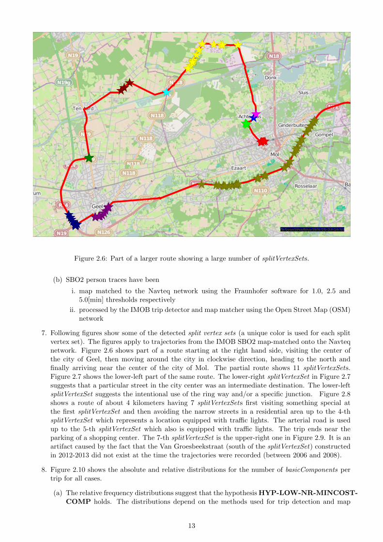
Figure 2.6: Part of a larger route showing a large number of splitVertexSets.
(b) SBO2 person traces have been
i. map matched to the Navteq network using the Fraunhofer software for 1.0, 2.5 and5.0[min] thresholds respectively
ii. processed by the IMOB trip detector and map matcher using the Open Street Map (OSM)network
7. Following figures show some of the detected split vertex sets (a unique color is used for each splitvertex set). The figures apply to trajectories from the IMOB SBO2 map-matched onto the Navteqnetwork. Figure 2.6 shows part of a route starting at the right hand side, visiting the center ofthe city of Geel, then moving around the city in clockwise direction, heading to the north andfinally arriving near the center of the city of Mol. The partial route shows 11 splitVertexSets.Figure 2.7 shows the lower-left part of the same route. The lower-right splitVertexSet in Figure 2.7suggests that a particular street in the city center was an intermediate destination. The lower-leftsplitVertexSet suggests the intentional use of the ring way and/or a specific junction. Figure 2.8shows a route of about 4 kilometers having 7 splitVertexSets first visiting something special atthe first splitVertexSet and then avoiding the narrow streets in a residential area up to the 4-thsplitVertexSet which represents a location equipped with traffic lights. The arterial road is usedup to the 5-th splitVertexSet which also is equipped with traffic lights. The trip ends near theparking of a shopping center. The 7-th splitVertexSet is the upper-right one in Figure 2.9. It is anartifact caused by the fact that the Van Groesbeekstraat (south of the splitVertexSet) constructedin 2012-2013 did not exist at the time the trajectories were recorded (between 2006 and 2008).
8. Figure 2.10 shows the absolute and relative distributions for the number of basicComponents pertrip for all cases.
(a) The relative frequency distributions suggest that the hypothesis HYP-LOW-NR-MINCOST-COMP holds. The distributions depend on the methods used for trip detection and map
13

Figure 2.7: Detail view of Figure 2.6 showing splitVertexSets in and near the city center.
Figure 2.8: Route showing splitVertexSets that correspond to traffic lights.
14

Figure 2.9: Detail of Figure 2.8 (rightmost part of the route).
matching. The distributions labeled Belgium Navteq x.y[min], differ only in the value fordelay threshold parameter used in stop-detection. The smaller the threshold value, the morestops are detected and hence the smaller the size of the trips (expressed as the number of linksthey contain). For a given sequence of GPS recordings, the more subsequences are flaggedas stops, the lower the number of detected basicPathComponents; this occurs because somebriefly visited locations will be flagged as a stop when using a small delay threshold parametervalue whereas they are detected to be a splitVertexSet in the opposite case. This is reflectedin the relative frequency distribution diagram. The probability (relative frequency) to findroutes having 1 basicPathComponent, decreases with increasing value of the delay parameter(1.0 , 2.5 , 5.0). For the case of 2 basicPathComponents the phenomenon is largely attenuated.Starting at 3 basicPathComponents per trip, the effect is reversed as expected.
(b) For Belgium, the OSM and Navteq cases seem to slightly differ. This can have been causedby the use of different map matching software tools, based on different methods and concepts.The Fraunhofer IAIS map matcher closes small gaps by assuming that the traveler used theshortest path. The IMOB map matcher does not use this procedure. This conclusion is notfinal because the cases differ both in the network and the map matcher used.
(c) The difference between the Belgian and Italian cases, however, is much larger. The relativefrequency for trips consisting of a single basicPathComponent is much larger than for thetrajectories registered in Belgium. For routes having more than one component, the relativefrequency is lower than in any Belgian case. Detail analysis is required to find out whetherthis phenomenon occurs because in the Italian data set, the pre- and post-car-trip componentsare missing.
9. Table 2.1 summarizes characteristics of the runs. The poor performance of the calc4 server wasexplained by an operating system mis-configuration and seems not to be specific to this application.
15

Absolute frequency distribution for the number of basicPathComponents for the 4 runs appliedto the Belgian trips.
Relative frequency distribution for the number of basicPathComponents for the 4 runs appliedto the Belgian trips.
Figure 2.10: Frequency distributions for the number of basicComponents per trip. The number of tripsin each set depends on the map matcher used.
16
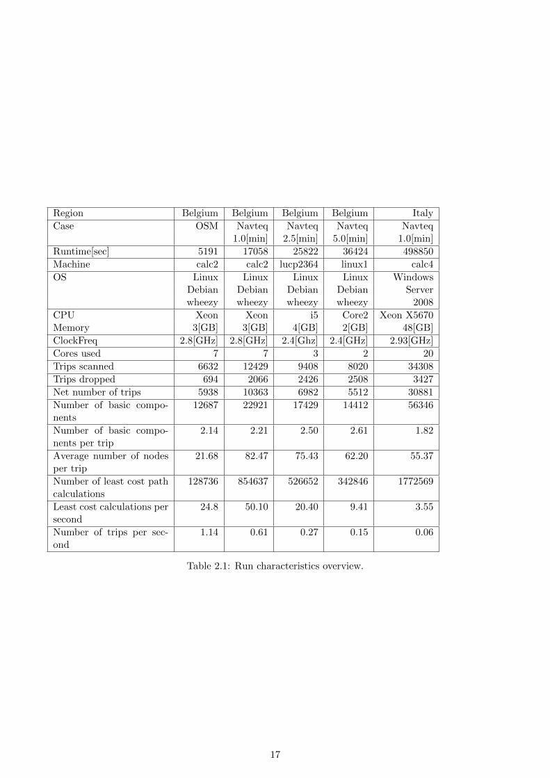
Region Belgium Belgium Belgium Belgium Italy
Case OSM Navteq Navteq Navteq Navteq1.0[min] 2.5[min] 5.0[min] 1.0[min]
Runtime[sec] 5191 17058 25822 36424 498850
Machine calc2 calc2 lucp2364 linux1 calc4
OS Linux Linux Linux Linux WindowsDebian Debian Debian Debian Serverwheezy wheezy wheezy wheezy 2008
CPU Xeon Xeon i5 Core2 Xeon X5670Memory 3[GB] 3[GB] 4[GB] 2[GB] 48[GB]
ClockFreq 2.8[GHz] 2.8[GHz] 2.4[Ghz] 2.4[GHz] 2.93[GHz]
Cores used 7 7 3 2 20
Trips scanned 6632 12429 9408 8020 34308
Trips dropped 694 2066 2426 2508 3427
Net number of trips 5938 10363 6982 5512 30881
Number of basic compo-nents
12687 22921 17429 14412 56346
Number of basic compo-nents per trip
2.14 2.21 2.50 2.61 1.82
Average number of nodesper trip
21.68 82.47 75.43 62.20 55.37
Number of least cost pathcalculations
128736 854637 526652 342846 1772569
Least cost calculations persecond
24.8 50.10 20.40 9.41 3.55
Number of trips per sec-ond
1.14 0.61 0.27 0.15 0.06
Table 2.1: Run characteristics overview.
17

2.1.3 Radiation Model in FEATHERS
The location choice model for work locations in FEATHERS has been replaced by the radiation lawdescribed in [SGMB12]. In this section we first compare the original location choice model used inFEATHERS and the radiation model. Then, simulation results for both models are compared.
2.1.3.1 Radiation model
The radiation model described in [SGMB12] applies to work locations (commuting). The number of jobopportunities in a region (city) is assumed to be proportional to the population. The model assumesthat a job request emitted from a given home location L0 is intercepted by a job opportunity in the sameor a different region. A request emitted from L0 is possibly intercepted by L1 6= L0 if and only if itwas not intercepted by L0 or by an intermediate location Li|Li 6= L0 ∧ Li 6= L1 ∧ d(L0, Li) ≤ d(L0, L1).Hence, the model is not based on distance but on a ranking of the opportunity locations using theirdistance to the home location.
2.1.3.2 Location choice in FEATHERS
The location choice model in FEATHERS is used for all activity types and hence applies to both fixed(mandatory) and flexible (discretionary) activities.
1. The model is used in to consecutive steps. At a coarse spatial level it is first used to determinethe municipality; in a finer grained level it is used to select a FEATHERS subzone within themunicipality. The location model has been described in paper [AHT03] and more elaborated inthe book [AT04a]. Note that the zoning terminology differs slightly from the one used in theoriginal paper [AHT03].
2. The method uses following concepts:
(a) order
(b) distance band
(c) distance ranking
3. In all cases order of an area is a rank number in a list where areas are sorted in ascending orderby a size attribute. Several different size attributes are used.
(a) For municipality order the size is the number of households residing in the area (not thenumber of individuals, see [AHT03]) which acts as a proxy for the population size. The rankis assumed to define a functional hierarchy of the cities/towns so that the highest rankedcities/towns expose a supra-regional function in terms of work, leisure and social activities.Lower ranked cities/towns have a local function only.
(b) For a zone, the size attribute to use depends on the activity type for which a location is tobe selected. For work activities, the relative employment opportunity level of the zone withinthe municipality is used as the size.
sw(z) =E(z)∑
z∈Z(M)
E(z)(2.1)
In (2.1) sw(z) denotes the value of the size attribute of zone z when it comes to work locationselection, Z(M) denotes the set of zones in municipality M and E(z) denotes the number ofemployments in zone z.
For all activity types, the size values are subdivided into 4 categories by specifying the bound-aries between the classes in terms of relative occurrence frequencies
order .class
4 5.0% largest zones with size > 03 10.5% second largest zones with size > 02 28.0% third largest zones with size > 01 56.5% remaining zones with size > 0
18

2.1.3.3 Models comparison for work location choice
The radiation model described in [SGMB12] is a single step model. In this model
• population size is used as a proxy for the number of job opportunities
• candidate locations are ranked according to their distance to the home location of the individualselecting a work location
The FEATHERS (Albatross) model described in [AHT03] and in [AT04b] is a two phase model. Eachphase consists of following steps:
• decision tree based selection by order
• decision tree based selection by distance band
• random selection by distance ranking
For the municipality level, the order is determined by ranking the regions using the number of residenthouseholds. For the subzone level, the relative size of employment is used to rank the alternativelocations.
Algorithm 2.1 has been derived from figure 2 in paper [AHT03] and shows the location choice pro-cedure. Names starting with DT denote methods that apply a decision tree based procedure to selecta result. The decision trees have been trained using survey data.
Algorithm 2.1 Location choice algorithm in FEATHERS (Albatross)
1: mun← currentMunicip2: if DT otherMun() then3: if DT homeMunicip() then4: mun← homeMun5: else6: nextLocMunOrder ← DT selectMunOrder()7: if DT nearestMunOfGivenOrder(nextLocMunOrder) then8: mun← munNearestToCurrentLocation(nextLocMunOrder)9: else
10: munDistBand← DT selectMunDistBand(nextLocMunOrder)11: munSet← selectMunSetByDistBand(currentMun,munDistBand, nextLocMunOrder)12: mun← selectFromMunSet(munSet)13: end if14: end if15: end if16: zoneOrderInMun← DT getOrderOfZoneToSelect()17: zoneDistBand← DT selectZoneDistBand(zoneOrderInMun)18: zoneSet← selectZoneSetByDistBand(mun, currentMun, currentZone, zoneDistBand, zoneOrderInMun)19: zone← selectFromZoneSet(zoneSet)
• Line 2 determines whether or not to execute the next activity in the municipality that containsthe current location.
• Line 4 finds out whether the next activity is to be performed in the individual’s home municipality
• Line 6 determines the order for the next municipality to select
• Line 7 determines whether the nearest municipality of the given order is to selected.
• Line 8 selects municipality of given order that is nearest to the current location
• Line 10 selects a distance band using a decision tree
19

• Line 11 selects municipalities of given order within the distance band
• Line 12 selects one municipality from the set by random selection based on distance ranking mech-anism
• Line 16 determines the order of the zone to select within the municipality
• Line 17 selects a distance band using a decision tree
• Line 18 selects set of zones of given order within the distance band
• Line 19 selects one zone from the set by random selection based on distance ranking mechanism
2.1.3.4 Replacement of the FEATHERS location choice model by radiation models
In order to compare the FEATHERS (Albatross, see section 2.1.3.3) and radiation models, the locationselection at municipality level has been replaced in FEATHERS. Details and experimental results havebeen reported in DLV4.2 section Radiation Model in FEATHERS
2.1.4 Doubly Constrained Location Choice Models
This section presents work on location choice models based on radiation and gravitation laws respectivelythat take saturation effects into account. In a constellation of requesters (the ones looking for a job)and providers (job opportunities) having a limited capacity, the state of each provider shall be takeninto account. This induces the effect of saturation which means that simple state ignoring models(neither gravitation nor radiation) are adequate. Therefore, doubly constrained models are proposed inthis section. For a given pair (requester,provider) those models are based on (1) the magnitude of thedemand, (2) the magnitude of the supply at a given moment in time (or equivalently at a given systemstate) and (3) a function based on attributes of the pair that characterize the attraction between requesterand provider. In the work location choice model case, those methods are based on the knowledge of thenumber of job seekers and of the number of remaining open job opportunities at a given moment in timein each location. The state variable remaining open job opportunities is ignored in the simpler models.
When considering doubly constrained models, the incoming and outgoing commuter flows are given.We started from a given commuter home-work OD matrix derived from census data for Flanders. Theaim is to reconstruct the OD matrix from the given row and column sums (numbers of outgoing andincoming commuters respectively). If this turns out to be possible, a location choice model for activitybased schedule generators can be built from the given marginals. Filling all cells in an OD matrix whenonly the row and column sums are given is a highly under-determined problem. The idea is to find outwhether reconstruction is feasible by making use of the corresponding known OD-impedance (distanceor travel duration) matrix.
In order to evaluate the usability of the radiation model in the location choice module of an activity-based schedule predictor, experiments using data for Flanders have been executed. The current locationchoice model used in FEATHERS is described in section 2.1.3.3. The aim is to find out whether it ispossible to reconstruct the origin-destination (OD) flow matrix from the row and columns sums by usingthe information contained in the radiation and gravity laws. If this would be the case, the reconstructedOD flow matrix can serve as a basis to sample (work) activity locations in the Monte Carlo simulationfor an activity-based model. The research is summarized in the following sub-sections.
2.1.4.1 Data used
A home-work flow matrix was derived from the SEE (Socio-Economische Enquete) dataset for Belgium.The SEE makes use of building blocks (BB) or statistical sectors. The average area for the buildingblocks in the Flanders region is 1.2[km2]. The dataset is based on following subdivisions of the studyarea:
20

Number Zoning : Level
20759 building blocks : 12815 subZones : 21314 zones : 3332 superZones, municipalities : 4
Each entity at a given level is completely contained in exactly one entity at the next higher level. Thearea of an entity is completely covered by all the areas at the next lower level it contains.
The experiments have been carried out at superZone level for following reasons: (i) the matricesfor the BB level are too large to run simulations on a 4GB laptop (ii) the simulations took too muchrun-time Building blocks are more or less homogeneous with respect to socio-demographic characteristicsand land-use (residential, business area, industry zoning, recreational, agricultural, etc). This does nothold at municipality level.
Distance was used as a measure for travel impedance. The given distances matrix contains thelength for shortest path between building blocks measured along the road network. This matrix wascondensed to a distance matrix at superZone level. The distance between two superZones szA and szBconsisting of the sets of building blocks bbA and bbB respectively, is defined by 1
N
∑a∈bbA,b∈bbB
d(a, b) with
N = |bbA| · |bbB| and d(a, b) the impedance (in this case: distance) to travel from the centroid of a tothe centroid of b along the network.
All home-work location pairs were extracted from the SEE data (and hence have been reported byindividuals).
2.1.4.2 Software: Principle of Operation
1. Only home-work travel between different zones is considered. Intra-zonal travel is ignored. Noother individual travel or activity is considered.
2. Software was developed to micro-simulate the location choice for each individual. During thesimulation, an individual is selected for processing by first sampling a superZone TAZ from theset of non-exhausted TAZ using a uniform distribution. A non-exhausted TAZ is a TAZ forwhich at least one more outgoing home-work trip needs to be assigned to a destination TAZ.This technique is used because individuals are not identified neither represented in the software.Sampling individuals from the population using a uniform distribution would require two steps:(i) sampling a TAZ from a distribution defined by the population size for the TAZ (ii) samplingan individual from the TAZ using a uniform distribution This technique was expected to take toomuch run-time. Since the TAZ are more or less equally populated, it is assumed that uniformlysampling the TAZ is sufficiently accurate (the sampling order affects the result due to saturationeffects by job opportunities being consumed).
3. As soon a an individual is sampled, the target (work) location is sampled using the techniquedescribed below in sections 2.1.4.3 and 2.1.4.4; then the number of job requesters in the homelocation Fout[h] and the number of remaining job opportunities Fin[t] in the target location aredecremented. As a consequence, no individuals can be drawn from an exhausted TAZ t (whereFout[t] = 0) neither be assigned to a saturated TAZ t (where Fin[t] = 0). The actual sizes of theremaining outgoing and incoming flows in each TAZ are used to feed the functions that determinethe assignment probabilities. Finally, each time a request is absorbed by a location, the home-workflow matrix is adapted. This is summarized by:
h← sampleHome()t← sampleTarget()Fout[h]← Fout[h]− 1Fin[h]← Fin[h]− 1HW [h][t]← HW [h][t] + 1
21

2.1.4.3 Gravity Model
A gravity model using the deterrence function f(d) = d−2 where d is the impedance between the TAZinvolved. The probability weight function for trips leaving TAZ torig is given by
p(tdest) =N(tdest) · α∑
ti∈TN(ti) · d2(torig, ti)
(2.2)
where α is a normalization factor, d(torig, ti) is the impedance to travel from torig to ti and N(t) is thenumber of remaining open job opportunities in t. A probability matrix P with ∀i ∈ |T | :
∑j∈|T |
p[i][j] = 1
is maintained.The probability matrix is not recalculated for each individual assignment but the populations is
subdivided in chunks and the matrix is recalculated each time a TAZ becomes saturated or a chunk hasbeen processed. For the experiments, 200 chunks were used.
2.1.4.4 Radiation Model
The radiation model is simulated by executing for each individual the emission-absorption process dis-cussed in [SGMB12] page 23.
Consider the level z of the emitted job request. It has a probability density f(z) that does not dependon the individual. For each request (outgoing commuter) the level is assumed to equal the maximumzmax,m value found after m extractions where m is the number of remaining outgoing commuters in theorigin location who are still looking for a job opportunity. In the same way, for a possible destinationlocation, the maximum value for the request level that can be absorbed, is determined a the maximumvalue in a set of n extractions from f(z) where n is the number of open job opportunities in the candidatedestination location.
Note that for every probability density function f(x) with (cumulative) distribution F (x) =∫f(x)dx,
the cumulative distribution for the maximum of k extractions, is given by F k(x). A value for themaximum is sampled by sampling u ∼ uniform(0, 1) and calculating x from
u = F k(x) (2.3)
x = F−1(u1k ) (2.4)
(2.5)
One needs to sample the maximum level for the emitter location and for the absorber location and todetermine whether the level for the emitter is lower than the one for the absorber.
xe = F−1(u1me ) (2.6)
xa = F−1(u1na ) (2.7)
xe ≤ xa ⇔ u1me ≤ u
1na (2.8)
⇔ log(ue)
m≤ log(ue)
n(2.9)
since F−1(x) is monotonically increasing in [0, 1]. See also [SGMB12].A value ue ∼ uniform(0, 1) is sampled for the emitter (origin) location. Then the potential desti-
nations are scanned in order of increasing travel impedance. A value ua ∼ uniform(0, 1) is sampled foreach candidate absorbing (destination) location and the first one for which the condition mentioned in(2.9) holds is selected to absorb the request.
It is possible that a request is not absorbed because the number of absorbers is finite. Therefore, thesoftware provide a fallback: the request is recycled after doubling the log(ue)
m value which means that themaximum value after m
2 extractions is considered. The number of times this was required for the 986931commuters for the experiments reported below, is shown in the table.
22

Figure 2.11: Scatter plot showing the correspondence between the given flow values and the flowscalculated using the gravitation law. The value for each off-diagonal cell in the home-work matrix isshown.
Number of Number of Adaptations Relative numberpeople adaptations per adapted person of people adapted
23437 45253 1.930 0.02423478 45046 1.918 0.02423242 44752 1.925 0.02423310 44830 1.923 0.024
2.1.4.5 Results
1. Radiation and gravitation models.Given and calculated OD-flow matrices are compared. For each OD-flow matrix, the diagonalelements specify the number of intra-TAZ trips; those numbers are given and hence identical in allmatrices (given and calculated ones). For comparisons, off-diagonal elements only are consideredbecause diagonal elements shall have no influence on the quality measure.
Figure 2.11 shows the scatter plot for tuples (HWcalc[o][d], HWgiven[o][d]) for all (o, d)|o 6= d pairs.HWgiven designates the given home-work flow matrix and HWcalc designates the matrix calculated(reconstructed) using the gravity law. Figure 2.12 shows the similar scatter plot for the matrixcalculated (reconstructed) using the gravity law. The correlation between given and reconstructedvalues (not their logarithms) ∀(o, d)|o 6= d is low in both cases as shown in following table. In aperfect reconstruction, all points should be on the line y = x.
Case R (Pearson) R2
Gravity 0.75585 0.57130Radiation 0.60983 0.37189
Figure 2.13 shows the frequency distribution for the distances found in the given and the calculatedhome-work OD flow matrices for a gravity model simulation. The red line represents the distribu-tion for the distances in the reconstructed OD flow matrix; the green line corresponds to the givenmatrix and the blue line shows the difference. The number of short distance trips is underesti-mated. Figure 2.14 shows the frequency distribution for the distances found in the given and the
23

Figure 2.12: Scatter plot showing the correspondence between the given flow values and the flowscalculated using the radiation law. The value for each off-diagonal cell in the home-work matrix isshown.
Figure 2.13: Probability density functions for the distance found in the given (green line) and calculated(red line) OD home-work flow matrices for the gravitation law case.The blue line shows the difference.
24

Figure 2.14: Probability density functions for the distance found in the given (green line) and calculated(red line) OD home-work flow matrices for the radiation law case. The blue line shows the difference.
calculated home-work OD flow matrices for a radiation model simulation. The red line representsthe distribution for the distances in the reconstructed OD flow matrix; the green line correspondsto the given matrix and the blue line shows the difference. The number of short distance tripsis over-estimated. In order to further compare the methods, four runs for the gravity case andfour runs for the radiation case have been executed. The off-diagonal elements are arranged ina N2 − N = N · (N − 1) dimensional vector. Using the scalar product, the cosine of the anglebetween vectors is used to evaluate the quality of the matrix reconstruction. This is similar tothe Pearson correlation coefficient but does not apply a translation to the exected value. Resultshave been summarized in the table below. Each row and each column in the table corresponds toa simulation run (using either the gravitation law or the radiation law). Each cell corresponds totwo checks and hence is associated with two vectors (matrices). The cell value is cos(α) where α isthe angle between the vectors. The table is symmetric. The first column/row corresponds to thegiven OD flow matrix.
Given Rad.1 Rad.2 Rad.3 Rad.4 Grav.1 Grav.2 Grav.3 Grav.4
Given 1.000000 0.612213 0.611238 0.612454 0.611430 0.760153 0.761436 0.759589 0.760234Radi.1 0.612213 1.000000 0.999428 0.999435 0.999414 0.573575 0.577157 0.574327 0.574533Radi.2 0.611238 0.999428 1.000000 0.999327 0.999405 0.573921 0.577609 0.574655 0.574953Radi.3 0.612454 0.999435 0.999327 1.000000 0.999425 0.573447 0.577071 0.574202 0.574446Radi.4 0.611430 0.999414 0.999405 0.999425 1.000000 0.574676 0.578347 0.575413 0.575733Grav.1 0.760153 0.573575 0.573921 0.573447 0.574676 1.000000 0.997460 0.997592 0.997496Grav.2 0.761436 0.577157 0.577609 0.577071 0.578347 0.997460 1.000000 0.997390 0.997452Grav.3 0.759589 0.574327 0.574655 0.574202 0.575413 0.997592 0.997390 1.000000 0.997468Grav.4 0.760234 0.574533 0.574953 0.574446 0.575733 0.997496 0.997452 0.997468 1.000000
The cosine values in the first row, show that the angle between each vector constructed using thegravitation law and the vector corresponding to the given flow matrix, is nearly the same for allsimulations. The same is observed for the vectors generated using the radiation law. The cosinevalues however are very small indicating that the vectors for the reconstructed flow matrix arealmost orthogonal to the vector corresponding to the given flow matrix.
The next rows also show the cosine values for the angles between the vector for all pairs of solutions.It is easily observed that a given law (gravitation or radiation) produces solutions corresponding to
25

vectors having almost the same direction. This means that the magnitude of stochastic effects ismuch smaller than the systematic error. On average, the angle α between radiation and gravitationsolutions is larger (cosα = 0.577) than between the solutions and the given vector (cosα = 0.612and cosα = 0.760 for the radiation and gravitation law respectively).
2. Radiation model with personal decision to reject opportunity.Since the small distance cases seem to be overestimated, an additional experiment was performed.The radiation law assumes that a TAZ is chosen as soon as region is found for which the sampledthe maximum required job level does not exceed the sampled maximum level for the available op-portunities. In such case, the TAZ is chosen as the destination location. The model was adaptedso that there is a given probability to reject the offered opportunity. The probability is identicalfor everyone. The software was run for values [0.02 . . . 0.30] using a 0.02 increment. The values forcosα and r are given in the table below and in Figure 2.15. Clearly, the values remain well belowthose found for the gravitation model.
Probability to reject cosα r(Pearson)
0.00 0.61477 0.612410.02 0.61589 0.613500.04 0.61992 0.617520.06 0.61891 0.616460.08 0.62665 0.624220.10 0.62884 0.626370.12 0.62894 0.626440.14 0.63227 0.629720.16 0.63760 0.635060.18 0.63942 0.636840.20 0.64050 0.637890.22 0.64111 0.638450.24 0.64166 0.638950.26 0.64410 0.641360.28 0.64413 0.641340.30 0.63941 0.63654
3. Predictions by FEATHERSA set of schedules was predicted by a FEATHERS run for half of the Flemish population (FRAC2).A home-work flow matrix was derived by considering every schedule that contains a work activity.The home location and the first trip arriving at the work location have been extracted to determinethe required matrix. This method is used because, in many cases, people travel to another locationbefore going to work. The values in the matrix have been doubled to get a prediction for the fullpopulation. Figure 2.16 shows the scatterplot where each point represents a tuple of a predicted andthe corresponding observed value. Please note that the given (observed) home-work flow matrixwas derived from the SEE census data for the year 2001 whereas the FEATHERS prediction wasproduced using data for 2010. The size of the FEATHERS predicted vector is 1.1613 times thelength of vector for the observed data; this can be caused by the fact that the observed (given)dataset holds for 2001 (SEE data) while the FEATHERS prediction holds for 2010. The vectorsize does not matter, the direction is important. On the other hand, there is no reason to believethat distribution of the trips over the OD-pairs has changed a lot during that period.
The cosα = 0.637957 value nearly equals the value for the radiation model with saturation andwith 18% probability for people not accepting the proposed opportunity (first or any subsequentproposal) but it shows that the OD-matrix reconstruction is less accurate than for the gravitymodel case. Figure 2.17 shows the probability density for the home-work distance. Clearly, theFEATHERS prediction for the distance is better that the one for any other method.
26
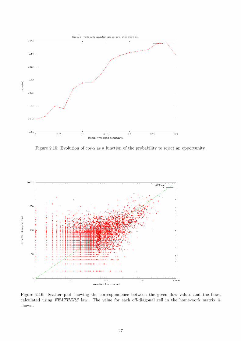
Figure 2.15: Evolution of cosα as a function of the probability to reject an opportunity.
Figure 2.16: Scatter plot showing the correspondence between the given flow values and the flowscalculated using FEATHERS law. The value for each off-diagonal cell in the home-work matrix isshown.
27

Figure 2.17: Probability density functions for the distance found in the given (green line) and calculated(red line) OD home-work flow matrices for the FEATHERS prediction case.The blue line shows the difference.
2.1.4.6 Discussion - Conclusion
1. Please note that the results about the integration of the radiation law in FEATHERS that have beenreported in section 2.1.3.4 and in deliverable D4.2 do not apply to flow matrices. In the section,the original radiation law (not the doubly constrained variant) was integrated in FEATHERS.The results presented in that section are numbers of jobs assigned to locations. Because thissection covers doubly constrained models, the number of jobs assigned to each zone (i.e. the sizeof the incoming flow) is given. This section focuses on the reconstruction of the flows (OD matrixelements). The problem is largely under-determined since only since for case of n locations thereare n2 unknowns and 2· equations. Location choice models essentially try to use some law in orderto compensate for the lack of equations.
2. Both the gravitation and radiation laws seem to be able to select locations so that the distributionsfor the home-work distance approximate the one found in the original data. However, neither ofboth is succeeds in reproducing the given OD flow matrix accurately which means that neitherof the laws by itself is sufficient to serve as a location choice model in an activity-based micro-simulator. Although the distance distributions seem to be realistic, none of the methods can beexpected to generate realistic flows. Clearly, some essential information is not captured by themodels.
This is explained by following factors:
(a) the homogeneity of the area. Municipalities cover the entire area of Flanders (i.e. there is notmuch empty space between municipality centers) and their population sizes are similar.
(b) the laws apply to the selection of a work location as a function of the travel impedance andfail to discriminate between locations having similar impedance values. In particular, anyinformation about job kinds is ignored since a single density function f(z) is used for the levelof requests and opportunities.
(c) the impedance values (travel distance, travel duration) are calculated between municipalitycentroids. In densely populated regions like Flanders, the distance between centroids is of thesame size as the radius of the TAZ.
28

(d) in cases where the impedance values and number of job opportunities are nearly equal, thecandidate TAZ in the gravity model have nearly equal probability to become selected. In suchcases, rank based models (like the radiation model) assigns a higher priority to particular zonesin a set where all zones have nearly equal impedance and number of job opportunities.
3. The OD-matrix reconstruction by the FEATHERS location choice model, performs as good as theradiation model but is not as accurate as the gravitation model.
Conclusion: impedance values combined with one of the investigated laws are not sufficient to recon-struct the OD flow matrix when the numbers of outgoing and incoming commuters for each TAZ aregiven. Please note that the methods have been evaluated using one given dataset of incoming andoutgoing home-work trips for the municipality level zoning of Flanders. The gravity based model us-ing a quadratic deterrence function, delivers the most accurate prediction for the OD-matrix and theFEATHERS location choice model delivers the best distance distribution.
2.1.5 Estimating the deterrence function for singly constraint gravity models
A non-parametric method to simultaneously estimate the weights (populations) and the deterrencefunction in single constrained gravity models is presented. This section reports research that is goingon and for which preliminary results only are available at the time of writing this DATASIM deliverableDLV3.2. The principle of the method is presented here, results will be presented only in the comingmonths.
2.1.5.1 Concept - Aim
The gravity model is the typical modeling framework used to estimate commuting trips between citiesor municipalities, and it has found wide application in the estimate of various kinds of spatial flows.Although there are many different formulations of gravity models, most of them estimate the averagenumber of trips from location i to j as
Tij ∝ wiwjf(rij , γ) (2.10)
where w is the weight, a local variable usually proportional to the resident population or the number ofjobs in a location, and the other is the distance, r, which depends on the pair of locations considered andcan be the geographic distance, the road distance, the travel time, the travel cost or other. f(r, γ) is thedeterrence function that depends on the parameter(s) γ and describes how flows decay with distance.Gravity models can be further classified based on the type of constraints that are imposed on theirestimates. In a single constrained model the total number of estimated departures from any locationi, Ti, is constrained to be equal to the total number of observed departures from i, T ∗i , Ti =
∑j Tij =∑
j T∗ij = T ∗i . In a doubly constrained model there is an additional constraint, ensuring that the total
number of estimated arrivals in each location is also equal to the total number of observed arrivals.
2.1.5.2 Method
Here we propose a general method to find the deterrence function and the values of weights that pro-vide an optimal estimate of the observed OD matrix, T ∗ij , using a single constrained gravity model.We compare the estimates of commuting trips in Flanders using our method with those obtained us-ing a doubly constrained model, and comment on the performances of the two methods in the discussion.
In single constrained gravity models the average number of trips from i to j is given by the followingequation
Tij = Tiwjf(rij , γ)∑j wjf(rij , γ)
= Ti pij(w, fγ) (2.11)
where pij(w, fγ) is the estimated probability of a trip from location i to j, and depends on the weightsand the deterrence function and its parameter(s). Due to the independence of individual trips, the
29

probability to observe a given sequence of trips from location i to all other locations, {tij}j , is given bythe multinomial distribution
P ({tij}|Ti, {pij}) = Ti!∏j 6=i
ptijij
tij !(2.12)
and the average number of trips between any two locations is indeed Tij = Tipij .Usually the weight is assumed to be proportional to the resident population or the number of jobs,
and in other cases it is assumed to be a function (usually a power law) of these variables. The deterrencefunction is usually assumed to be power law, exponential, stretched exponential or a more complexfunction. Our method will seek to find the single constrained gravity model that provides the bestestimate of the observed flows, i.e. the model with the shortest L1 distance from the data,
∑ij |T ∗ij−Tij |.
The difference of our approach with respect to other methods in the literature is that we do not make any apriori assumption on the functional form of weights and deterrence function. In particular, weights do notexplicitly depend on population or any other socio-economic variable, but are treated as free parameters.Similarly, the deterrence function is estimated using a non-parametric regression, i.e. without pre-imposing a particular functional form but expressing it as a sum of 10 gaussians whose parameters(amplitude, mean, and variance) are free parameters. Our method thus consists in looking for the valuesof the n weights and the parameters of the 10 gaussians (i.e. n+ 30 total parameters) that minimize thesum of the absolute differences between model and data trips.
Starting from a uniform set of values for the free parameters, we iterate over the following steps:
1. Optimize the deterrence function: Keeping the weights fixed, the downhill simplex algorithm isused to find the parameters of the 10 gaussians {Ak, µk, σk}10k=1 that minimize the cost function∑
ij |T ∗ij − Tij |:
minγ
∑i 6=j
∣∣T ∗ij − Ti pij (w, fγ)∣∣ = (2.13)
min{Ak,µk,σk}10k=1
∑i 6=j
∣∣∣∣∣T ∗ij − Ti pij(
w,10∑k=1
Ake−
(rij−µk)2
σk
)∣∣∣∣∣ (2.14)
2. Optimize the weights: Keeping the deterrence function’s parameters fixed, the downhill simplexalgorithm is used to find the weights w that minimize the cost function
∑ij |T ∗ij − Tij |:
minw
∑i 6=j
∣∣T ∗ij − Ti pij (w, fγ)∣∣ (2.15)
Steps 1. and 2. are repeated until the final values of the parameters do not significantly vary withrespect to the initial values (typically when they have not changed more than 1%).
2.2 Prediction of Travel Time from Big Data
The travel time and travel volume between regions were derived from recorded GPS traces. This tech-nique allows for direct observation of so-called volume delay functions (VDF) for use in the trafficassignment (network loading) procedure.
Details about this work have been reported in WP4 because in a first stage, the results serve forvalidation of predicted travel demand on arterial relations. Nevertheless, the results can be used in theprediction phase too. Preparing a road network for use in simulations is expensive because a volume-delay function (VDF) needs to be assigned to each link. Several such functions are in use and all ofthem require parameters. Discussions about which function to use last for a long time. The VDF cannotbe derived solely from the characteristics of the cross-section of the road. Longitudinal characteristics,
30

curvature, slope and land use also are important. The multitude of required data makes the job to definean accurate network description expensive.
The method used in this research subdivides the study area using a Voronoi tesselation which defines avirtual network for which VDF have been determined for each link (for details : see deliverable DLV4.2).The tessels can (in the worst case interactively) be mapped to TAZ. The virtual network allows todetermine the time dependent travel time between TAZ directly from observations. This is exactly whatis required by activity-based schedule predictors. In the current state of the art, the travel times arecalculated by
1. assigning VDF parameters to each link; the parameters are determined using rules of thumb fromthe road characteristics
2. loading the estimated traffic demand to the network (traffic assignment)
3. skim the network to determine the expected travel time for each origin destination TAZ pair
This process is to be repeated for different travel demand situations (off-peak, morning-peak, evening-peak) which makes it a costly procedure. Furthermore, the estimated travel demand is required as aninput (but that is exactly what is to be determined by the activity-based schedule generator. Hence, theprocess is to be executed in a loop until sufficient convergence. This typically can take multiple hoursor even days of computation time.
Being able to observe the VDF directly from recorded data could be a less expensive and moreaccurate solution to construct the actual accessibility network (accessibility relation between locations)for a new study area. Observing the VDF in the study area solves the question of which area to considerfor network skimming in the method described above. In order to define traffic volumes, transit demand(trips not starting nor ending in the study area) needs to be taken into account. As a consequence, inthe method described above, the area for which to estimate the initial travel demand shall be larger thanthe study area. Determination of this surrounding area is more an art than a science. This problem issolved in an efficient way by direct observation of the VDF.
2.3 Schedule Adaptation
Schedule adaptation research focuses on short term (e.g. unexpected non recurring congestion) and longterm (e.g. adaptation to cooperation in carpooling and additional constraints imposed by EV) cases.
2.3.1 WIDRS: Within-Day Rescheduling
FEATHERS is a schedule predictor. It generates agendas for individuals before the start of the day.WIDRS is a schedule execution simulator that supports adaptation of partially executed schedules.
1. People are assumed to maximize utility when adapting their schedule. In the current WIDRSversion, utility is assumed to depend on the duration of the activity only (hence not on the absolutetime). Marginal utility is assumed to monotonically decrease with the duration of the activity.Those rules together define the mechanism for time compression/expansion of activities.
2. In general, in a single day simulator, schedules can be adapted by re-timing (compression/expansionof duration), re-ordering of activities, re-location of activities, mode change and activity dropping.WIDRS currently supports re-timing only.
3. Papers [KUB+12] and [KUB+13] describe in detail how the coefficients for the (marginal) utilityfunctions are determined from the hypothesis of predicted schedule optimality.
4. WIDRS was first used to estimate the effect of a large scale unexpected congestion on the roadnetwork. The road network performance in Flanders (i.e. the travel duration for each possibleOD-pair (origin,destination locations pair) is calculated using a macroscopic traffic assignment(stochastic user equilibrium) for each 15[min] period of the day. Hence, the network performanceis specified by 96 travel duration matrices (impedance matrices).
31

5. Since FEATHERS predictions are based on only 3 impedance matrices (off-peak, morning-peak,evening-peak) the predicted schedules initially have to be (slightly) adapted using so that thetravel times in the schedules correspond to the travel times supported by the network. Since traveltimes are adapted, activity times will change. The utility functions mentioned before are used andan iteration is run to establish an equilibrium between traffic demand and supply w.r.t. traveldurations planned by the individuals and the ones provided by the network infrastructure. Theequilibrium is found after 3 iterations.
6. After that, schedule execution simulation starts. In one of the investigated cases, a incident duringthe morning peak was simulated. The incident is modeled by reducing the capacity of the roadsegments in a given set for a given period of time. The effect emerges in the travel times calculatedfor the next 15[min] period. Notifications about the changed network performance are assumed tobe emitted by a broadcast mechanism. Some people are on the road and possibly are subjected tothe extra congestion (experiencing travelers). People who are not yet on the road either (1) receivethe information on time and can reschedule or (2) miss the message and start traveling.This ismodeled by perception filters. As soon as someone becomes aware of the extra congestion, (s)heestimates the new travel times using individual-specific parameters and managed by the perceptionfilter and reschedules the remainder of the day. This can lead to abruptly stopping the currentactivity.
7. In WIDRS, time resolution for activity/trip start/end is 1[min] but due to the macroscopic trafficassignment, individuals can re-estimate travel times only every quarter of an hour.
2.3.2 EVC-WIDRS: Rescheduling in order to optimize EV charging cost
1. New modules have been added to create EVC-WIDRS (EV charging WIDRS). It serves to simulateEV using individuals. They try to charge their batteries at the lowest possible cost.
2. Travel times are calculated once; recalculation is not relevant in this context and has been droppedbecause it is very time consuming. The utility maximization mechanism using the same monoton-ically decreasing marginal utility functions, has been retained.
3. The individual can buy electric energy at a time dependent cost that is communicated to allinterested individuals at once (i.e. simultaneously) and once every 24[h] (day-ahead predictioncompatible with the scheme used in section Coordinating EV charging in balancing powermarkets in the WP6 deliverable).
4. Following cases have been considered:
(a) with respect to grid capacity
i. there are no grid constraints with respect to power transmission
ii. grid constraints apply: since it is not possible to acquire sufficient power grid describingdata, UPM assembled a synthetic grid for Flanders (see WP6 deliverable section FlemishTransmission Grid Description).
(b) with respect to behavior
i. business as usual scenario: People do not adapt their schedules, use the EV in the sameway they used their ICEV (internal combustion engine vehicle) before and the EV logicnegotiates with the distributor to get the battery charged during specific time slots norder to minimize the cost.
ii. the case where individuals accept to adapt their schedules by shifting activity start andend time over one or two quarters of an hour in order to find a lower cost solution thanthe one found in item 4(b)i. The cost savings are compared to the utility loss caused byre-timing. Relative savings and relative utilities are compared in order to avoid the VOT(value of time) problem. Absolute cost saving is also compared with absolute shifts intime and drop utility drop. More details have been reported in deliverable DLV6.
(c) In all cases
32

i. the assumptions with respect to the charger power, car specific energy consumption andthe possibility to charge at work are the same as the ones mentioned in [KKB+12]
ii. all required chargers are available at all times (i.e. no queueing problem, no competitionto use a plug)
iii. each car logic is supplied with information about time dependent cost and time dependentavailable power in each TAZ (traffic analysis zone)
2.3.3 Cooperation in Activity-based Models
Current activity-based models do not model cooperation. In the first subsection, we explain the need toexplicitly model cooperation. In the second subsection, an agent-based simulator focusing on carpoolingis presented.
2.3.3.1 The need to model cooperation between entities
Current activity-based models predict cooperative actions (social visits, driving as a passenger) executedby individuals by means of stochastic sampling but without verifying the feasibility. Predicted resultsare not necessarily consistent; e.g. carpooling for commuting with someone who is not a householdmember is predicted with verifying whether a companion is available to travel between the respectivelocations at the specified times (home-work and work-home trips). For many applications, a limited levelof inconsistency does not matter (e.g. to estimate the car flow entering specific zones during specificperiods). However. the effect of some TDM (Travel Demand Management) measures might heavilydepend on the possibility to coordinate and cooperate.
Modeling coordination and cooperation require the use of agent-based models. Consider followingexample: realistic EV charging simulation can benefit agent-based modeling because of the requiredcoordination consumers, aggregators, distributors and producers of electric energy (even in the casewhere consumers are assumed to act independently).
In order to calculate the lower and upper limits as well as the expected values of specific quantities,one needs to know their inter-dependencies. It is well known that in some applications involving a largenumber of similar entities, the mechanisms governing the behavior exposed by the complete set might beunknown while the interactions between individuals can be investigated and formally specified. In suchcases, the agent-based modeling technique can elicit emergent effects and allow for their quantification.As an example, consider a set of EV users who charge their batteries via a smartgrid that is partiallyfed by wind and solar power sources.
1. The EV users travel via a network for which the variability of travel time is quite large and forwhich local local service level disturbances (due to incidents) can induce a loss of time that is ofthe same order of magnitude as the originally predicted required travel time for normal conditions.
2. Execution periods for locally executes activities also have stochastic duration.
3. In general, not all details in daily plans (schedules) are predicted one-day-ahead. People tend topredict (plan) a skeleton, start executing the schedule and re-plan details about flexible activitiesduring schedule execution.
4. Wind and solar power can show large variability. Energy storage capacity is very limited and thetransport capacity is limited by grid constraints (both by network nodes and links).
5. Energy distributors can provide price reduction to people offering charging flexibility by promisingconnection periods longer than what is required to charge the required amount of energy. Theyexpect commitments by consumers and charge a penalty for shortening the promised connectiontime or for shifting connection time periods back and forth.
6. Not all communications between consumers and the smartgrid entities do occur at once (becausenot everyone is expected to be connected at the same moment in time and because communicationbandwidth is limited). Furthermore for the reason mentioned in item 3, planning data comesavailable in small chinks at any time of the day.
33

Calculating the emergent behavior (e.g. power peak demand mitigation) of such complex system usingknowledge of its constituent components (humans, machines, meteorological phenomena) requires theuse of agent-based models. To evaluate the behavior of such system, a schedule execution simulator isrequired where individuals plan the future using receding horizon and convey information to the gridwhen it comes available and is sufficiently stable (to avoid to become penalized).
2.3.3.2 Agent based model for carpooling
In the DATASIM project it was decided to investigate problems (and their solutions) related to largescale agent-based models deployment by focusing on the problem of carpooling.
1. A problem statement is presented in the working report [KG13]. This is a problem specificationand model design document. It gives and overview of the submodels that define several aspectsof carpooling. It also list sources for data to feed the sub-models and indicates how the datacan be used. Finally, it reports on models for exploration (how to find carpooling companions),negotiation and schedule adaptation.
Related work is presented in internal reports produced by as DATASIM work documents [Kna12],[KKY+12], [KYC+13], [GYK+13], [KKY+13], [KYCB14], [GYK+14], [KBAHK+14]. Some of thematerial already resulted in published or submitted papers.
2. A prototype has been designed and implemented; it lead to the submission of a conference paper[HKB+15].
(a) The objectives were
i. to study the evaluation over time of the participation level in carpooling when a givenfraction of the population intends to carpool
ii. to find out the spatial distribution of effective carpoolers when the fraction of interestedpeople is spatially constant
iii. to investigate scalability issues when deploying large amounts of agents in an existingframework
In particular, carpooling for commuting was considered.
(b) The open source Janus framework (http://www.janus-project.org/) developed by UTBM wasused. This framework provides the organization concept as a type (i.e. not an instance). Anorganization represents an entity that can be joined by agents. The behavior of an agentsparticipating in organizations is specified by roles. A particular agent can participate in severalorganizations simultaneously. An agent joins an organization by specifying which role(s) itwill play. A group can be viewed as an instance of an organization.
3. Data for the experiment were taken from a set of schedules generated by FEATHERS. Peoplehaving schedules in which the home-work trip was followed by the work home trip without anyintermediate visit to any other location, were selected. The home and work locations have beenspecified as TAZ (Traffic Analysis Zone, average area about 5[km2]) not as street addresses. Peopleworking in the home location are assumed not to carpool (because of the short distance to travel).People are considered for carpool pairing only if they live in the same TAZ and work in the sameTAZ.
4. Exploration: an interested individual who is not carpooling, is assumed to explore for partnersby contacting people who fulfill the requirements mentioned in item 3. For each simulated day,the probability that the individual will explore, is specified in advance. The agent is allowedto send a limited number of invitations during each day for which it decides to explore. If anindividual receives an invitation, (s)he accepts the invitation for negotiation unless (s)he is alreadyparticipating in a carpool for which the car has no spare capacity. Hence, for a given invitation,a new carpool can be set up or an existing one can be extended. In the first experiment, eachindividual can be a member of at most one carpool at a given time and hence does not exploreas long as (s)he is participating in a carpool. In the exploration phase, the agent specifies the
34

Figure 2.18: Evolution of the number of individuals involved in carpooling over the simulated period fordifferent values of the acceptable trip start time adjustment.
preferred trip start times as well as the acceptable time windows (by specifying maximal negativeand positive adjustments to the preferential value).
5. Negotiation and schedule adaptation: the current model uses following trivial negotiationmechanism:
(a) both the home-work and work-home trips are considered in a single negotiation;
(b) the start time for the joint trips is the average value of the preferred trip start time commu-nicated by each candidate;
(c) negotiation succeeds if the trip start time is included in the acceptable time interval for everycandidate participant;
If the negotiation fails, no pool is formed or the existing pool remains unchanged. If negotiationsucceeds, a new pool is formed or the existing one is extended (the new candidate joins the pool).
6. Carpoolers are assumed to leave the pool after a finite period, determined by random selectionfrom a given distribution. When someone leaves the pool, the pool continues to exist with fewerparticipants unless its size dropped below two.
7. The Janus organization concept is used (i) to model the carpools with their driver and passengerroles, (ii) to model the sets of people sharing both home and work locations (for technical per-formance related reasons: Janus provides a facility to restrict the target audience for messages tothe collection of role players in a given organization) and finally (iii) to introduce the notion ofsimulated time (concept of a day) in the model.
8. The simulation starts with a given fraction of the population (30% in the experiment) beinginterested to explore and negotiate for carpooling. The first experiment was carried out using 65000agents (on a standard laptop with 4GB of memory). The preferential trip start time expressedby the individual, is the trip start time predicted for the solo trip by FEATHERS. The timingadjustment thresholds were identical for all agents. The simulation was run for three adjustmentlimit values: 10[min], 20[min] and 30[min] respectively. All cars have capacity 4 (driver included).The probability that an interested non-carpooling individual explores, equals 1 for every workingday. The number of invitations that can be emitted by each agent during a single day equals islimited to 5. The duration of the carpool participation is sampled uniformly in the range [20,30]working days (4 to 6 weeks). The evolution of the number of individuals involved in a carpool isshown in Figure 2.18 while the number of carpools is shown in Figure 2.19. By combining bothdiagrams, one can derive that car occupation increases when the time adjustment window grows.
35

Figure 2.19: Evolution of the number of cars involved in carpooling over the simulated period for differentvalues of the acceptable trip start time adjustment.
36
Bibliography
[AHT03] Theo A Arentze, Frank Hofman, and Harry J.P Timmermans. Re-induction of albatross’decision rules using pooled activity-travel diary data and an extended set of land use andcosts-related condition states. In TRB 2003 Annual Meeting, Washington, DC, USA,2003. Transportation Research Board.
[AT04a] Theo A Arentze and Harry J.P Timmermans. Albatross version 2: A learning-BasedTransportation Oriented Simulation System. European Institute of Retailing and ServicesStudies, Eindhoven, 2004.
[AT04b] Theo A Arentze and Harry J.P Timmermans. A learning-based transportation orientedsimulation system. Transportation Research Part B: Methodological, 38(7):613 – 633,2004.
[BKJ+14] Qiong Bao, Bruno Kochan, Davy Janssens, Tom Bellemans, and Geert Wets. Geograph-ical extension of the activity-based modeling framework FEATHERS. In Procedia Com-puter Science, Hasselt, June 2014.
[GYK+13] Stephane Galland, Ansar-Ul-Haque Yasar, Luk Knapen, Nicolas Gaud, Davy Janssens,Olivier Lamotte, Geert Wets, and Abderrafiaa Koukam. Multi-agent simulation of individ-ual mobility behavior in carpooling using the janus and JaSim platforms. TransportationResearch Part C, 2013.
[GYK+14] Stephane Galland, Ansar Yasar, Luk Knapen, Nicolas Gaud, Tom Bellemans, and DavyJanssens. Simulation of carpooling agents with the janus platform. Journal of UbiquitousSystems and Pervasive Networks (JUSPN), 2014.
[HKB+15] Iftikhar Hussain, Luk Knapen, Tom Bellemans, Davy Janssens, and Geert Wets. Anagent-based negotiation model for carpooling: A case study for flanders (belgium). InTRB 2015 Annual Meeting, Washington, DC, USA, 2015. TRB (Transportation ResearchBoard).
[HVK+15] Sylvia Heyvaert, Lieselot Vanhaverbeke, Luk Knapen, Katrien Declercq, Thierry Coose-mans, and Joeri Van Mierlo. Choosing an electric vehicle as a travel mode: Travel diarycase study in a belgian living lab context. In TRB 2015 Annual Meeting, Washington,DC, USA, 2015. TRB (Transportation Research Board).
[Jan11] Davy Janssens. FP7-ICT-2009-c data science for simulating the era of electric vehicles(ICT FET open call) part b. STREP Proposal FP7-ICT-2009.8.0 nr 270833, Transporta-tion Research Institute (IMOB), Diepenbeek, Belgium, March 2011.
[KBAHK+14] Luk Knapen, Irith Ben-Arroyo Hartman, Daniel Keren, Ansar Yasar, Sungjin Cho, TomBellemans, Davy Janssens, and Geert Wets. Scalability issues in optimal assignment forcarpooling. JCSS (Journal of Computer and System Sciences), 2014.
[KBAHS+14] Luk Knapen, Irith Ben-Arroyo Hartman, Daniel Schulz, Davy Janssens, Tom Bellemans,and Geert Wets. Determining structural route components from GPS traces. Paper inpreparation, Hasselt University Transportation Institute (IMOB), Diepenbeek, Belgium,2014.
37

[KBJW14a] Luk Knapen, Tom Bellemans, Davy Janssens, and Geert Wets. Canonic route splitting.Diepenbeek, Belgium, February 2014.
[KBJW14b] Luk Knapen, Tom Bellemans, Davy Janssens, and Geert Wets. Map matching GPS tracesby sub-network selection (provisional title). Paper in preparation, 2014.
[KG13] Luk Knapen and Stephane Galland. Design note : Agent-based carpooling model. IMOBinternal report, Hasselt University Transportation Institute (IMOB), Diepenbeek, Bel-gium - Belfort, France, June 2013.
[KJY13] Luk Knapen, Davy Janssens, and Ansar-Ul-Haque Yasar. D3.1 behaviourally-sensitivesimulator design ready for the calculation of mobility-EV scenarios. Technical report,Hasselt University Transportation Institute (IMOB), Diepenbeek, Belgium, August 2013.
[KKB+12] Luk Knapen, Bruno Kochan, Tom Bellemans, Davy Janssens, and Geert Wets. Usingactivity-based modeling to predict spatial and temporal electrical vehicle power demandin flanders. Transportation Research Record, 2012.
[KKBJ14] Luk Knapen, Bruno Kochan, Tom Bellemans, and Davy Janssens. Notes on the use ofradiation laws in simulation. IMOB DataSIM research report, Hasselt University Trans-portation Institute (IMOB), Diepenbeek, Belgium, July 2014.
[KKY+12] Luk Knapen, Daniel Keren, Ansar-Ul-Haque Yasar, Sungjin Cho, Tom Bellemans, DavyJanssens, and Geert Wets. Analysis of the co-routing problem in agent-based carpoolingsimulation. In Procedia Computer Science, volume 10, pages 821 – 826, 2012. ANT 2012and MobiWIS 2012.
[KKY+13] Luk Knapen, Daniel Keren, Ansar Yasar, Sungjin Cho, Tom Bellemans, Davy Janssens,and Geert Wets. Estimating scalability issues while finding an optimal assignment forcarpooling. In Procedia Computer Science, Halifax, Nova Scotia, Canada, June 2013.Procedia Computer Science, Elsevier.
[Kna12] Luk Knapen. Notes on collaboration - carpooling model. IMOB internal report, IMOB,Diepenbeek, Belgium, June 2012.
[Kna13] Luk Knapen. Data used to feed schedule generators (data4simulation). IMOB DataSIMresearch report, IMOB, Diepenbeek, Belgium, November 2013.
[KU13] Luk Knapen and Muhammad Usman. Notes on EV-charging and ReScheduling simula-tion. IMOB internal report, Hasselt University Transportation Institute (IMOB), Diepen-beek, Belgium, May 2013.
[KUB+12] Luk Knapen, Muhammad Usman, Tom Bellemans, Davy Janssens, and Geert Wets.Framework to evaluate rescheduling due to unexpected events in an activity-based model.In TRB 2013 Annual Meeting, Washington, D.C., 2012.
[KUB+13] Luk Knapen, Muhammad Usman, Tom Bellemans, Davy Janssens, and Geert Wets.Within day rescheduling microsimulation combined with macrosimulated traffic. Trans-portation Research Part C, 2013.
[KYC+13] Luk Knapen, Ansar Yasar, Sungjin Cho, Daniel Keren, Abed Abu Dbai, Tom Bellemans,Davy Janssens, Geert Wets, Assaf Schuster, Izcak Sharfman, and Kanishka Bhaduri. Ex-ploiting graph-theoretic tools for matching in carpooling applications. Journal of AmbientIntelligence and Humanized Computing, 2013.
[KYCB14] Luk Knapen, Ansar-Ul-Haque Yasar, Sungjin Cho, and Tom Bellemans. Agent-basedmodeling for carpooling. In Data Science and Simulation in Transportation Research. IGIGlobal, Hasselt, DataSIM davy janssens, ansar-ul-haque yasar, luk knapen edition, 2014.
38

[RKD+15] Ali Raza, Luk Knapen, Katrien Declercq, Sylvia Heyvaert, Tom Bellemans, DavyJanssens, and Geert Wets. Diary survey quality assessment using GPS traces. InTRB 2015 Annual Meeting, Washington, DC, USA, 2015. TRB (Transportation ResearchBoard).
[SGMB12] Filippo Simini, Marta Gonzales, Amos Maritan, and Albert-Laszlo Barabasi. A universalmodel for mobility and migration patterns. Nature, 484(7392):96–100, April 2012.
[Sim14] Filippo Simini. A non-parametric method to estimate weights and deterrence functionin single constrained gravity models. Paper in preparation, Department of EngineeringMathematics, University of Bristol, Merchant Venturers Building, Woodland Road, BS81UB, Bristol, UK, Bristol, 2014.
[UKB+14] Muhammad Usman, Luk Knapen, Tom Bellemans, Davy Janssens, and Geert Wets. Effectof electrical vehicles charging cost optimization over charging cost and travel timings.Paper in preparation, IMOB, Diepenbeek, Belgium, 2014.
[UKY+14] Muhammad Usman, Luk Knapen, Ansar Yasar, Tom Bellemans, Davy Janssens, andGeert Wets. A framework for electric vehicle charging strategy optimization tested fortravel demand generated by an activity-based model. In Paper in preparation, Vienna,July 2014.
39