Concepts of Model Verification and Validation

LA-14167-MSApproved for public release;

distribution is unlimited.

This report was prepared as an account of work sponsored by an agency of the United StatesGovernment. Neither the Regents of the University of California, the United States Government norany agency thereof, nor any of their employees make any warranty, express or implied, or assumeany legal liability or responsibility for the accuracy, completeness, or usefulness of any information,apparatus, product, or process disclosed, or represent that its use would not infringe privately ownedrights. Reference herein to any specific commercial product, process, or service by trade name,trademark, manufacturer, or otherwise does not necessarily constitute or imply its endorsement,recommendation, or favoring by the Regents of the University of California, the United StatesGovernment, or any agency thereof. The views and opinions of authors expressed herein do notnecessarily state or reflect those of the Regents of the University of California, the United StatesGovernment, or any agency thereof. Los Alamos National Laboratory strongly supports academicfreedom and a researcher's right to publish; as an institution, however, the Laboratory does notendorse the viewpoint of a publication or guarantee its technical correctness.

Los Alamos National Laboratory, an affirmative action/equal opportunity employer, is operated by theUniversity of California for the United States Department of Energy under contract W-7405-ENG-36.

This work was supported by the National Nuclear Security Agency (NNSA),US Department of Energy (DOE), Office of Defense Programs.

Edited by Charmian Schaller, IM-1.

Concepts of Model Verification and Validation

Ben H. Thacker*

Scott W. Doebling

Francois M. Hemez

Mark C. Anderson

Jason E. Pepin

Edward A. Rodriguez

* Southwest Research Institute

LA-14167-MSIssued: October 2004

v

ABSTRACT

Model verification and validation (V&V) is an enabling methodology for the development of computational models

that can be used to make engineering predictions with quantified confidence. Model V&V procedures are needed by

government and industry to reduce the time, cost, and risk associated with full-scale testing of products, materials,

and weapon systems. Quantifying the confidence and predictive accuracy of model calculations provides the

decision-maker with the information necessary for making high-consequence decisions. The development of

guidelines and procedures for conducting a model V&V program are currently being defined by a broad spectrum of

researchers. This report reviews the concepts involved in such a program.

Model V&V is a current topic of great interest to both government and industry. In response to a ban on the

production of new strategic weapons and nuclear testing, the Department of Energy (DOE) initiated the Science-

Based Stockpile Stewardship Program (SSP). An objective of the SSP is to maintain a high level of confidence in

the safety, reliability, and performance of the existing nuclear weapons stockpile in the absence of nuclear testing.

This objective has challenged the national laboratories to develop high-confidence tools and methods that can be

used to provide credible models needed for stockpile certification via numerical simulation.

There has been a significant increase in activity recently to define V&V methods and procedures. The U.S.

Department of Defense (DoD) Modeling and Simulation Office (DMSO) is working to develop fundamental

concepts and terminology for V&V applied to high-level systems such as ballistic missile defense and battle

management simulations. The American Society of Mechanical Engineers (ASME) has recently formed a Standards

Committee for the development of V&V procedures for computational solid mechanics models. The Defense

Nuclear Facilities Safety Board (DNFSB) has been a proponent of model V&V for all safety-related nuclear facility

design, analyses, and operations. In fact, DNFSB 2002-11 recommends to the DOE and National Nuclear Security

Administration (NNSA) that a V&V process be performed for all safety related software and analysis.

Model verification and validation are the primary processes for quantifying and building credibility in numerical

models. Verification is the process of determining that a model implementation accurately represents the developer’s

conceptual description of the model and its solution. Validation is the process of determining the degree to which a

model is an accurate representation of the real world from the perspective of the intended uses of the model. Both

verification and validation are processes that accumulate evidence of a model’s correctness or accuracy for a

specific scenario; thus, V&V cannot prove that a model is correct and accurate for all possible scenarios, but, rather,

it can provide evidence that the model is sufficiently accurate for its intended use.

1 Letter from John T. Conway (Chairman, Defense Nuclear Facilities Safety Board) to Spencer Abraham (Secretary of Energy) dated 23 September 2002.

vi

Model V&V is fundamentally different from software V&V. Code developers developing computer programs

perform software V&V to ensure code correctness, reliability, and robustness. In model V&V, the end product is a

predictive model based on fundamental physics of the problem being solved. In all applications of practical interest,

the calculations involved in obtaining solutions with the model require a computer code, e.g., finite element or finite

difference analysis. Therefore, engineers seeking to develop credible predictive models critically need model V&V

guidelines and procedures.

The expected outcome of the model V&V process is the quantified level of agreement between experimental data

and model prediction, as well as the predictive accuracy of the model. This report attempts to describe the general

philosophy, definitions, concepts, and processes for conducting a successful V&V program. This objective is

motivated by the need for highly accurate numerical models for making predictions to support the SSP, and also by

the lack of guidelines, standards and procedures for performing V&V for complex numerical models.

vii

ACRONYMS

AIAA American Institute of Aeronautics and Astronautics

ANS American Nuclear Society

ANSI American National Standards Institute

ASCI Accelerated Strategic Computing Initiative

ASME American Society of Mechanical Engineers

ASQ American Society for Quality

BRP Blue Ribbon Panel

CVP Containment Vessel Program

DMSO Defense Modeling and Simulation Office

DNFSB Defense Nuclear Facilities Safety Board

DoD Department of Defense

DOE Department of Energy

FSI Fluid-structure interaction

HE High explosive

HSLA High-strength, low-alloy

IEEE Institute of Electrical and Electronics Engineers

ISO International Organization for Standardization

LANL Los Alamos National Laboratory

LLNL Lawrence Livermore National Laboratory

LSTC Livermore Software Technology Corporation

NAFEMS International Association for the Engineering Analysis Community

NASA National Aeronautics and Space Administration

NNSA National Nuclear Security Administration

NRC Nuclear Regulatory Commission

ODE Ordinary differential equation

PAS Performance Assurance System

PDE Partial differential equation

SCS Society for Computer Simulation

SNL Sandia National Laboratories

SRAC Structural Research & Analysis Corporation

SSP Stockpile Stewardship Program

SwRI Southwest Research Institute

USA Underwater shock analysis

V&V Verification and Validation

VCP Vessel Certification Package

viii

GLOSSARY

Accreditation .................................. Official certification that a model is acceptable for use for a specific purpose (DOD/DMSO, 1994).

Adequacy........................................ The decision that the model fidelity is sufficient for the intended use. Calculation Verification ................. Process of determining the solution accuracy of a particular calculation. Calibration...................................... Process of adjusting numerical or physical modeling parameters in the

computational model for the purpose of improving agreement with experimental data.

Calibration Experiment .................. Experiment performed for the purpose of fitting (calibrating) model parameters.

Certification.................................... Written guarantee that a system or component complies with its specified requirements and is acceptable for operational use (IEEE, 1990).

Code ............................................... Computer implementation of algorithms developed to facilitate the formulation and approximate solution of a class of models.

Code Verification ........................... Process of determining that the computer code is correct and functioning as intended.

Computer Model............................. Numerical implementation of the mathematical model, usually in the form of numerical discretization, solution algorithms, and convergence criteria.

Conceptual Model .......................... Collection of assumptions, algorithms, relationships, and data that describe the reality of interest from which the mathematical model and validation experiment can be constructed.

Confidence ..................................... Probability that a numerical estimate will lie within a specified range. Error ............................................... A recognizable deficiency in any phase or activity of modeling and

simulation that is not due to lack of knowledge. Experiment ..................................... Observation and measurement of a physical system to improve fundamental

understanding of physical behavior, improve mathematical models, estimate values of model parameters, and assess component or system performance.

Experimental Data .......................... Raw or processed observations (measurements) obtained from performing an experiment.

Experimental Outcomes ................. Measured observations that reflect both random variability and systematic error.

Experiment Revision ...................... The process of changing experimental test design, procedures, or measurements to improve agreement with simulation outcomes.

Fidelity ........................................... The difference between simulation and experimental outcomes. Field Experiment ............................ Observation of system performance under fielded service conditions. Inference......................................... Drawing conclusions about a population based on knowledge of a sample. Irreducible Uncertainty................... Inherent variation associated with the physical system being modeled. Laboratory Experiment................... Observation of physical system performance under controlled conditions. Mathematical Model....................... The mathematical equations, boundary values, initial conditions, and

modeling data needed to describe the conceptual model. Model ............................................. Conceptual/mathematical/numerical description of a specific physical

scenario, including geometrical, material, initial, and boundary data. Model Revision .............................. The process of changing the basic assumptions, structure, parameter

estimates, boundary values, or initial conditions of a model to improve agreement with experimental outcomes.

Nondeterministic Method............... An analysis method that quantifies the effect of uncertainties on the simulation outcomes.

Performance Model ........................ A computational representation of a model’s performance (or failure), based usually on one or more model responses.

Prediction ....................................... Use of a model to foretell the state of a physical system under conditions for which the model has not been validated.

Pretest Calculations ........................ Use of simulation outcomes to help design the validation experiment.

ix

Reality of Interest ........................... The particular aspect of the world (unit problem, component problem, subsystem or complete system) to be measured and simulated.

Reducible Uncertainty .................... Potential deficiency that is due to lack of knowledge, e.g., incomplete information, poor understanding of physical process, imprecisely defined or nonspecific description of failure modes, etc.

Risk ................................................ The probability of failure combined with the consequence of failure. Risk Tolerance................................ The consequence of failure that one is willing to accept. Simulation ...................................... The ensemble of models—deterministic, load, boundary, material,

performance, and uncertainty—that are exercised to produce a simulation outcome.

Simulation Outcome....................... Output generated by the computer model that reflect both the deterministic and nondeterministic response of the model.

Uncertainty ..................................... A potential deficiency in any phase or activity of the modeling or experimentation process that is due to inherent variability (irreducible uncertainty) or lack of knowledge (reducible uncertainty).

Uncertainty Quantification ............. The process of characterizing all uncertainties in the model and experiment, and quantifying their effect on the simulation and experimental outcomes.

Validation ....................................... The process of determining the degree to which a model is an accurate representation of the real world from the perspective of the intended uses of the model. (AIAA, 1998)

Validation Experiment.................... Experiments that are performed to generate high-quality data for the purpose of validating a model.

Validation Metric ........................... A measure that defines the level of accuracy and precision of a simulation. Verification..................................... The process of determining that a model implementation accurately

represents the developer’s conceptual description of the model and the solution to the model. (AIAA, 1998)

x

xi

TABLE OF CONTENTS

ABSTRACT ............................................................................................................................................................. v

ACRONYMS ........................................................................................................................................................... vii

GLOSSARY............................................................................................................................................................. viii

TABLE OF CONTENTS ......................................................................................................................................... xi

1.0 INTRODUCTION .......................................................................................................................................... 1 1.1 Background and Motivation.................................................................................................................. 1 1.2 Objective ............................................................................................................................................... 3 1.3 Approach............................................................................................................................................... 4

2.0 VERIFICATION AND VALIDATION PHILOSOPHY ............................................................................... 5

3.0 VERIFICATION ASSESSMENT .................................................................................................................. 10 3.1 Code Verification .................................................................................................................................. 10 3.2 Calculation Verification ........................................................................................................................ 11

4.0 VALIDATION ASSESSMENT ..................................................................................................................... 13 4.1 Validation Hierarchy............................................................................................................................. 14 4.2 Validation Metrics................................................................................................................................. 16 4.3 Validation Experiments......................................................................................................................... 17 4.4 Uncertainty Quantification.................................................................................................................... 19 4.5 Validation Requirements and Acceptable Agreement .......................................................................... 21

5.0 MODEL AND EXPERIMENT REVISION................................................................................................... 22

6.0 SUMMARY AND CONCLUSIONS ............................................................................................................. 24

ACKNOWLEDGMENTS ........................................................................................................................................ 25

REFERENCES ......................................................................................................................................................... 27

xii

1

1.0 INTRODUCTION

1.1 Background and Motivation

Current arms control agreements have provided the impetus for national directives to cease production of new

strategic weapons and end nuclear testing. In response to this challenge, the U.S. Department of Energy (DOE)

initiated the Science-Based Stockpile Stewardship Program (SSP). An objective of the SSP is to maintain a high

level of confidence in the safety, reliability, and performance of the existing nuclear weapons stockpile in the

absence of nuclear testing. This objective has challenged the national laboratories to develop high-confidence tools

and methods needed for stockpile certification via numerical simulation. Models capable of producing credible

predictions are essential to support the SSP certification goal. The process of establishing credibility requires a

well-planned and executed Model Verification and Validation (V&V) program.

The current ban on nuclear testing does not include experiments that are either nonexplosive—using a pulsed

reactor, for example—or subcritical, involving no self-sustaining nuclear reaction. Over the past 30 years,

Los Alamos National Laboratory (LANL), under the auspices of DOE, has been conducting confined high explosion

experiments to develop a better understanding of the behavior of materials under extremely high pressures and

temperatures. These experiments are usually performed in a containment vessel to prevent the release of explosion

products to the environment. Vessel designs utilize sophisticated and advanced three-dimensional (3D) numerical

models that address both the detonation hydrodynamics and the vessel’s highly dynamic nonlinear structural

response. It is of paramount importance that numerical models of the containment vessels be carefully developed

and validated to ensure that explosion products and debris from detonations of high-explosive assembly experiments

are confined and to produce a high level of confidence and credibility in predictions made with the models.

The Dynamic Experimentation (DX) Division at LANL has the overall responsibility for design, analysis,

manufacture, and implementation of new high-strength, low-alloy steel containment vessels. Because numerical

models are used in the design of containment vessels, a model V&V process is needed to guide the development of

the models and to quantify the confidence in predictions produced by these models. The expected outcome of the

model V&V process is the quantified level of agreement between experimental data and model prediction, as well

as the predictive accuracy of the model. This outcome is intended to provide a sound and technically defensible

basis to support decisions regarding containment-vessel certification. It is important to note that while the LANL

DynEx Vessel Program motivated the development of this report, the concepts presented here are general and

applicable to any program requiring the use of numerical models.

2

Verification and validation are the primary processes for quantifying and building confidence (or credibility) in

numerical models. The V&V definitions used in this report are adopted from the 1998 AIAA Guide, Ref. [1]:

• Verification is the process of determining that a model implementation accurately represents the

developer’s conceptual description of the model and the solution to the model.

• Validation is the process of determining the degree to which a model is an accurate representation of

the real world from the perspective of the intended uses of the model.

Verification and validation are processes that collect evidence of a model’s correctness or accuracy for a specific

scenario; thus, V&V cannot prove that a model is correct and accurate for all possible conditions and applications,

but, rather, it can provide evidence that a model is sufficiently accurate. Therefore, the V&V process is completed

when sufficiency is reached.

Verification is concerned with identifying and removing errors in the model by comparing numerical solutions to

analytical or highly accurate benchmark solutions. Validation, on the other hand, is concerned with quantifying the

accuracy of the model by comparing numerical solutions to experimental data. In short, verification deals with the

mathematics associated with the model, whereas validation deals with the physics associated with the model. [9]

Because mathematical errors can eliminate the impression of correctness (by giving the right answer for the wrong

reason), verification should be performed to a sufficient level before the validation activity begins.

Software V&V is fundamentally different from model V&V. Software V&V is required when a computer program

or code is the end product. Model V&V is required when a predictive model is the end product. A code is the

computer implementation of algorithms developed to facilitate the formulation and approximate solution of a class

of models. For example, ABAQUS or DYNA3D permit the user to formulate a specific model, e.g., the DynEx

vessel subjected to internal blast loading with specific boundary conditions, and effect an approximate solution to

that model. A model includes more than the code. A model is the conceptual/mathematical/numerical description of

a specific physical scenario, including geometrical, material, initial, and boundary data.

The verification activity can be divided into code verification and calculation verification. When one is performing

code verification, problems are devised to demonstrate that the code can compute an accurate solution. Code

verification problems are constructed to verify code correctness, robustness, and specific code algorithms. When one

is performing calculation verification, a model that is to be validated is exercised to demonstrate that the model is

computing a sufficiently accurate solution. The most common type of calculation-verification problem is a grid

convergence study to provide evidence that a sufficiently accurate solution is being computed.

3

Numerical models can be used to simulate multiple and/or coupled physics such as solid mechanics, structural

dynamics, hydrodynamics, heat conduction, fluid flow, transport, chemistry, and acoustics. These models can

produce response measures such as stress, strain, or velocity time histories, or failure measures such as crack

initiation, crack growth, fatigue life, net section rupture, or critical corrosion damage. For example, a DYNA3D

response model can compute a stress time history that is used as input to a crack-growth model to compute fatigue

life. The model will also include input and algorithms needed to quantify the uncertainties associated with the

model.

Model V&V is undertaken to quantify confidence and build credibility in a numerical model for the purpose of

making a prediction. Ref. [1] defines prediction as “use of a computational model to foretell the state of a physical

system under conditions for which the computational model has not been validated.” The predictive accuracy of the

model must then reflect the strength of the inference being made from the validation database to the prediction.

If necessary, one can improve the predictive accuracy of the model through additional experiments, information,

and/or experience.

The requirement that the V&V process quantify the predictive accuracy of the model underscores the key role of

uncertainty quantification in the model-validation process. Nondeterminism refers to the existence of errors and

uncertainties in the outputs of computational simulations due to inherent and/or subjective uncertainties in the

model. Likewise, the measurements that are made to validate these simulation outcomes also contain errors and

uncertainties. While the experimental outcome is used as the reference for comparison, the V&V process does not

presume the experiment to be more accurate than the simulation. Instead, the goal is to quantify the uncertainties in

both experimental and simulation results such that the model fidelity requirements can be assessed (validation) and

the predictive accuracy of the model quantified.

1.2 Objective

The objective of this report is to provide the philosophy, general concepts, and processes for conducting a successful

model V&V program. This objective is motivated by the need for highly accurate numerical models for making

predictions to support the SSP and by the current lack of guidelines, standards, and procedures for performing model

V&V.

This report has been developed to meet the requirements of the DynEx Project Quality Assurance Program [2],

which defines implementation of DOE Order 414.1A, Chg. 1: 7-12-01, Quality Assurance, and Code of Federal

Regulation, Title 10 CFR Ch. III (1–1–02 Edition) Subpart A—Quality Assurance Requirements 830.120 Scope,

830.121 Quality Assurance Program, and 830.122 Quality Assurance Criteria, and section 5.6 – Design Control of

DynEx Quality Assurance Plan, DV-QAP. This report meets, in part, DNFSB Recommendation 2002-1, Quality

Assurance for Safety-Related Software. The DynEx Vessel Project leader, DX-5 group leader, and the DX division

leader are responsible for implementation of this report.

4

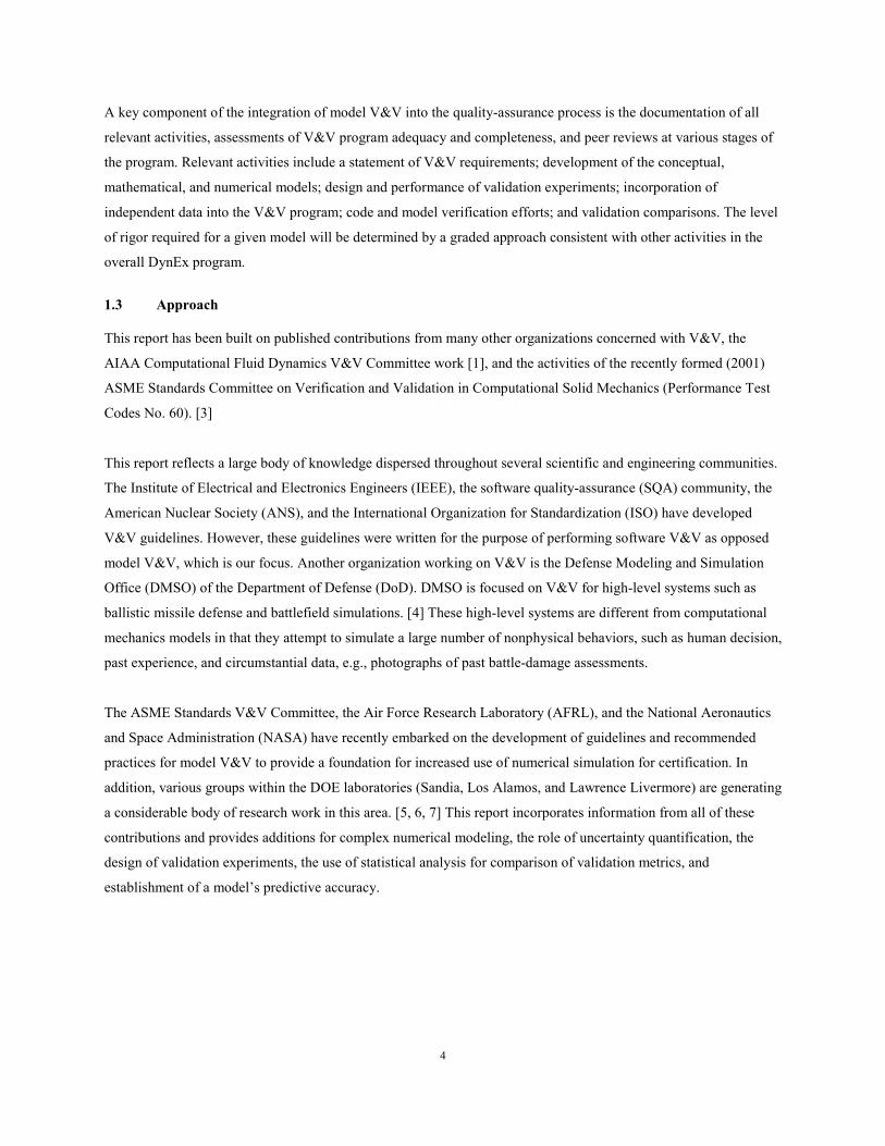
A key component of the integration of model V&V into the quality-assurance process is the documentation of all

relevant activities, assessments of V&V program adequacy and completeness, and peer reviews at various stages of

the program. Relevant activities include a statement of V&V requirements; development of the conceptual,

mathematical, and numerical models; design and performance of validation experiments; incorporation of

independent data into the V&V program; code and model verification efforts; and validation comparisons. The level

of rigor required for a given model will be determined by a graded approach consistent with other activities in the

overall DynEx program.

1.3 Approach

This report has been built on published contributions from many other organizations concerned with V&V, the

AIAA Computational Fluid Dynamics V&V Committee work [1], and the activities of the recently formed (2001)

ASME Standards Committee on Verification and Validation in Computational Solid Mechanics (Performance Test

Codes No. 60). [3]

This report reflects a large body of knowledge dispersed throughout several scientific and engineering communities.

The Institute of Electrical and Electronics Engineers (IEEE), the software quality-assurance (SQA) community, the

American Nuclear Society (ANS), and the International Organization for Standardization (ISO) have developed

V&V guidelines. However, these guidelines were written for the purpose of performing software V&V as opposed

model V&V, which is our focus. Another organization working on V&V is the Defense Modeling and Simulation

Office (DMSO) of the Department of Defense (DoD). DMSO is focused on V&V for high-level systems such as

ballistic missile defense and battlefield simulations. [4] These high-level systems are different from computational

mechanics models in that they attempt to simulate a large number of nonphysical behaviors, such as human decision,

past experience, and circumstantial data, e.g., photographs of past battle-damage assessments.

The ASME Standards V&V Committee, the Air Force Research Laboratory (AFRL), and the National Aeronautics

and Space Administration (NASA) have recently embarked on the development of guidelines and recommended

practices for model V&V to provide a foundation for increased use of numerical simulation for certification. In

addition, various groups within the DOE laboratories (Sandia, Los Alamos, and Lawrence Livermore) are generating

a considerable body of research work in this area. [5, 6, 7] This report incorporates information from all of these

contributions and provides additions for complex numerical modeling, the role of uncertainty quantification, the

design of validation experiments, the use of statistical analysis for comparison of validation metrics, and

establishment of a model’s predictive accuracy.

5

2.0 VERIFICATION AND VALIDATION PHILOSOPHY

A high level schematic of the V&V process is shown in Figure 1. This graphical representation is a derivative of a

diagram developed by the Society for Computer Simulation (SCS) in 1979 and is referred to as the Sargent Circle.

[8] This diagram provides a simplistic illustration of the modeling and simulation activities (black solid lines) and

the assessment activities (red dashed lines) involved in Model V&V.

In Figure 1, the Reality of Interest represents the physical system for which data is being obtained. Later in this

report we will describe a hierarchy of experiments for building the validation database, beginning with simple

(single physics) unit problems and ending with the complete system. Consequently, the Reality of Interest represents

the particular problem being studied, whether a unit problem, component problem, subsystem, or the complete

system. The V&V of a complete system will necessarily require the process shown in Figure 1 to be repeated

multiple times as the model development progresses from unit problems to the complete system.

The Mathematical Model comprises the conceptual model, mathematical equations, and modeling data needed to

describe the Reality of Interest. The Mathematical Model will usually take the form of the partial differential

equations (PDEs), constitutive equations, geometry, initial conditions, and boundary conditions needed to describe

mathematically the relevant physics.

Figure 1: Simplified view of the model verification and validation process. [8]

6

The Computer Model represents the implementation of the Mathematical Model, usually in the form of numerical

discretization, solution algorithms, miscellaneous parameters associated with the numerical approximation, and

convergence criteria. The Computer Model comprises the computer program (code), conceptual and mathematical

modeling assumptions, code inputs, constitutive model and inputs, grid size, solution options, and tolerances.

Additionally, the Mathematical and Computer Model may include a performance (or failure) model, as well as an

uncertainty analysis method, solution options, and tolerances.

The process of selecting important features and associated mathematical approximations needed to represent the

Reality of Interest in the Mathematical Model is termed Modeling. Assessing the correctness of the Modeling is

termed Confirmation. The Verification activity focuses on the identification and removal of errors in the Software

Implementation of the Mathematical Model.

As will be discussed in more detail in a subsequent section, Verification can be divided into at least two distinct

activities: Code Verification and Calculation Verification. Code Verification focuses on the identification and

removal of errors in the code. Calculation Verification focuses on the quantification of errors introduced during

application of the code to a particular simulation. Arguably, the most important Calculation Verification activity is

performing a grid or time convergence study (successively refining the mesh or time step until a sufficient level of

accuracy is obtained).

As the final phase, the Validation activity aims to quantify the accuracy of the model through comparisons of

experimental data with Simulation Outcomes from the Computer Model. Validation is an ongoing activity as

experiments are improved and/or parameter ranges are extended. In the strictest sense, one cannot validate a

complete model but rather a model calculation or range of calculations with a code for a specific class of problems.

Nevertheless, this report will use the more widely accepted phrase “model validation” instead of the correct phrase

“calculation validation.”

Although Figure 1 is effective for communicating the major concepts involved in model V&V, several important

activities are not shown. Figure 1 does not clearly represent 1) the various activities involved in designing,

performing, and presenting experimental results; 2) the parallel and cooperative role of experimentation and

simulation, 3) the quantification of uncertainties in both experimental and simulation outcomes, and 4) an objective

mechanism for improving agreement between experiment and simulation. Figure 2 expands on Figure 1, providing

more detail to address these and other shortcomings.

In Figure 2, the right branch illustrates the process of developing and exercising the model, and the left branch

illustrates the process of obtaining relevant and high-quality experimental data via physical testing. The closed

boxes denote objects or data, connectors in black solid lines denote modeling or experimental activities, and the

connectors in dashed red lines denote assessment activities.

7

Modeling, Simulation, &Experimental Activities

Assessment Activities

Code & Calculation Verification

Conceptual Model

Conceptual Model

Validation Experiment

Validation Experiment

Experimental Data

Experimental Data

Experimental Outcomes

Experimental Outcomes

ComputerModel

ComputerModel

Simulation Outcomes

Simulation Outcomes

MathematicalModel

MathematicalModel

Pre-test Calculations

Acceptable Agreement?

Next Reality of Interest

Experimentation

Quantitative Comparison

Implementation

Uncertainty Quantification

No

Yes

Reality of Interest

Reality of Interest

Abstraction

Revise Model or Experiment

Uncertainty QuantificationModel

Validation

Physical Modeling Mathematical Modeling

Modeling, Simulation, &Experimental Activities

Assessment Activities

Modeling, Simulation, &Experimental Activities

Assessment Activities

Code & Calculation Verification

Conceptual Model

Conceptual Model

Validation Experiment

Validation Experiment

Experimental Data

Experimental Data

Experimental Outcomes

Experimental Outcomes

ComputerModel

ComputerModel

Simulation Outcomes

Simulation Outcomes

MathematicalModel

MathematicalModel

Pre-test Calculations

Acceptable Agreement?

Next Reality of Interest

Experimentation

Quantitative Comparison

Implementation

Uncertainty Quantification

No

Yes

Reality of Interest

Reality of Interest

Abstraction

Revise Model or Experiment

Uncertainty QuantificationModel

Validation

Physical Modeling Mathematical Modeling

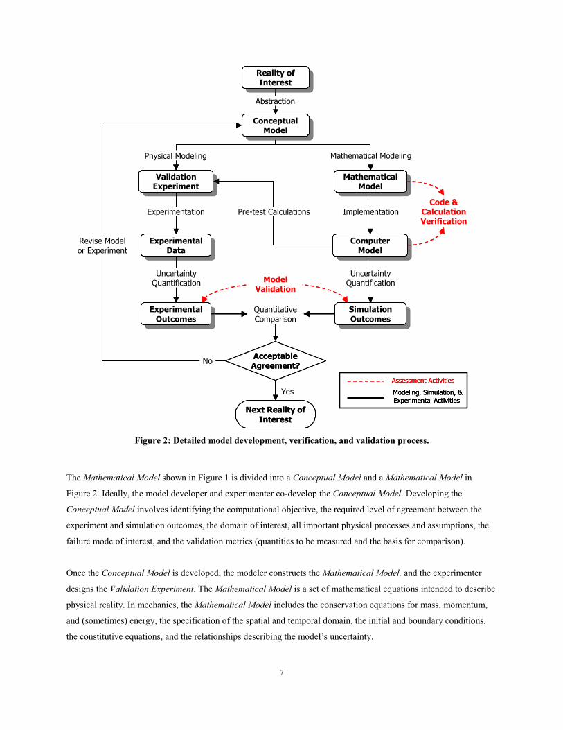
Figure 2: Detailed model development, verification, and validation process.

The Mathematical Model shown in Figure 1 is divided into a Conceptual Model and a Mathematical Model in

Figure 2. Ideally, the model developer and experimenter co-develop the Conceptual Model. Developing the

Conceptual Model involves identifying the computational objective, the required level of agreement between the

experiment and simulation outcomes, the domain of interest, all important physical processes and assumptions, the

failure mode of interest, and the validation metrics (quantities to be measured and the basis for comparison).

Once the Conceptual Model is developed, the modeler constructs the Mathematical Model, and the experimenter

designs the Validation Experiment. The Mathematical Model is a set of mathematical equations intended to describe

physical reality. In mechanics, the Mathematical Model includes the conservation equations for mass, momentum,

and (sometimes) energy, the specification of the spatial and temporal domain, the initial and boundary conditions,

the constitutive equations, and the relationships describing the model’s uncertainty.

8

The Computer Model is the implementation of the equations developed in the Mathematical Model, usually in the

form of numerical discretization, solution algorithms, and convergence criteria. The Computer Model is generally a

numerical procedure (finite element, finite difference, etc.) for solving the equations prescribed in the Mathematical

Model with a computer code. The codes used for mechanics problems typically include methods for discretizing the

equations in space and time, along with algorithms for solving the approximate equations that result.

A portion of the Computer Model represents the nondeterministic solution method, uncertainty characterizations,

and associated convergence criteria. Typical nondeterministic theories include probabilistic methods, fuzzy sets,

evidence theory, etc. Uncertainties are characterized in the form of the model used to represent the uncertainty—for

example, a probability distribution used to represent the variation in elastic modulus, or intervals used to represent

bounded inputs. Uncertainty Quantification is performed to quantify the effect of all input and model form

uncertainties on the computed simulation outcomes. Thus, in addition to the model response, Simulation Outcomes

include quantified error (or confidence) bounds on the computed model response.

Code and Calculation Verification assessments are performed on the Computer Model to identify and eliminate

errors in programming, insufficient grid resolution, solution tolerances, and finite precision arithmetic. Code and

Calculation Verification are discussed in detail in a subsequent section.

On the experimental (left) side of Figure 2, a physical experiment is conceived and designed. The result is a

Validation Experiment. The purpose of a Validation Experiment is to provide information needed to validate the

model; therefore, all assumptions must be understood, well defined, and controlled in the experiment. To assist with

this process, Pretest Calculations (including sensitivity analysis) can be performed, for example, to identify the most

effective locations and types of measurements needed from the experiment. These data will include not only

response measurements, but also measurements needed to define model inputs and model input uncertainties

associated with loadings, initial conditions, boundary conditions, etc. For example, load and material variabilities

can be quantified by the symmetrical placement of sensors within an experiment, and test-to-test variations can be

quantified by performing multiple validation experiments.

The Pretest Calculations link between the experimental and computational branches in Figure 2 also reflects the

important interaction between the modeler and the experimenter that must occur to ensure that the measured data is

needed, relevant, and accurate. Once the Validation Experiment and Pretest Calculations are completed, however,

the modeler and experimenter should work independently until reaching the point of comparing outcomes from the

experiment and the simulation.

9

Experimentation involves the collection of raw data from the various sensors used in the physical experiment

(strain and pressure gauges, high speed photography, etc.) to produce Experimental Data such as strain

measurements, time histories of responses, videos, photographs, etc. If necessary, experimental data can be

transformed into experimental “features” to be more directly useful for comparison to simulation results. To support

the quantification of experimental uncertainties, repeat experiments are generally necessary to quantify the lack of

repeatability due to systematic error (bias) and uncontrollable variability.

Uncertainty Quantification is then performed to quantify the effect of measurement error, design tolerances, as-built

uncertainties, fabrication errors, and other uncertainties on the Experimental Outcomes. Experimental Outcomes

typically take the form of experimental data with error bounds as a function of time or load.

Uncertainty Quantification is shown on both left and right branches of Figure 2 to underscore its important role in

quantifying the uncertainty and confidence in both the experimental and simulation outcomes. The Quantitative

Comparison of Experimental and Simulation Outcomes may take the form of a statistical statement of the selected

validation metrics. For example, if the validation metric were the difference between the simulation and

experimental outcome (or simply “error”), the Quantitative Comparison would quantify the expected accuracy of

the model, e.g., “We are 95% confident that the error is between 5% and 10%.” Validation metrics are discussed in

more detail in a subsequent section.

The Model Validation assessment determines the degree to which a model is an accurate representation of the real

world from the perspective of the intended uses of the model. This information is used to decide whether or not the

model has resulted in Acceptable Agreement with the experiment. The question of whether or not the model is

adequate for its intended use is broader than implied in the Acceptable Agreement decision block shown in Figure 2.

The Acceptable Agreement decision focuses only on the level of agreement between Experimental and Simulation

Outcomes, the criteria for which were specified as part of the Conceptual Model.

If the agreement between the experimental and simulation outcomes is unacceptable, the model and/or the

experiment can be revised. Model revision is the process of changing the basic assumptions, structure, parameter

estimates, boundary values, or initial conditions of a model to improve agreement with experimental outcomes.

Experiment revision is the process of changing experimental test design, procedures, or measurements to improve

agreement with simulation outcomes. Whether the model or the experiment (or both) are revised depends upon the

judgment of the model developer and experimenter.

In the following sections, we describe in more detail the various simulation, experimental, and assessment activities

illustrated in Figure 2.

10

3.0 VERIFICATION ASSESSMENT

Verification is the process of determining that a model implementation accurately represents the developer’s

conceptual description of the model and the solution to the model. [1] In performing verification, it is useful to

divide the verification activity into distinct parts (Table 1), recognizing the different function of software developers

producing a code that is error free, robust, and reliable, and model developers who use the code to obtain solutions

to engineering problems with sufficient accuracy. [11]

Table 1: Verification assessment classifications and descriptions.

Classification Focus Responsibility Methods

Software Quality Assurance

Reliability and robustness of the software

Code developer & Model developer

Configuration management, static & dynamic testing, etc.

Code Verification Numerical

Algorithm Verification

Correctness of the numerical algorithms in the code

Model developer Analytical solutions, benchmark problems, manufactured solutions, etc.

Calculation Verification

Numerical Error Estimation

Estimation of the numerical accuracy of a given solution to the governing equations

Model developer Grid convergence, time convergence, etc

3.1 Code Verification

The purpose of code verification is to confirm that the software is working as intended. The main focus of this

activity is to identify and eliminate programming and implementation errors within the software (software quality

assurance) and to verify the correctness of the numerical algorithms that are implemented in the code (numerical

algorithm verification); therefore, code verification is the responsibility of both the code developer and the model

developer.

Code verification is partially accomplished using software quality assurance (SQA) procedures. SQA performed by

the code developer is used to ensure that the code is reliable (implemented correctly) and produces repeatable results

on specified computer hardware, operating systems, and compilers. SQA is typically accomplished using

configuration management and static and dynamic software quality testing. SQA procedures are needed during the

software development process, and during production computing.

11

Model developers should also perform SQA by running all relevant verification problems provided with the

software. This approach not only provides evidence that the model developer can correctly operate the code but also

helps to ensure that executing the code on the model developer’s computer system reproduces the results obtained

by the code developers executing the code on their computer systems. This recommended practice has also been

called “confirmation.” [9]

Code verification also encompasses checking the implementation of numerical algorithms used in the code, a

process referred to as numerical algorithm verification. In this activity, test problems with known (analytical) or

highly accurate (benchmark) solutions are devised and compared to solutions obtained with the code. In the absence

of highly accurate solutions, a technique termed the “method of manufactured solutions” (MMS) can be used to

create analytical solutions that are highly sensitive to programming and algorithmic errors. [10]

In general, uncertainty quantification is performed using software, so code verification is also required for the

uncertainty analysis algorithms. This process entails comparing computed solutions to known or highly accurate

nondeterministic solutions. Benchmark solutions can be obtained, for example, by using Monte Carlo simulation

with a large number of samples. These solutions can be saved and reused as established probabilistic benchmark

solutions.

Since it cannot be proven that a code is error free, the accumulation of well-thought-out test cases provides evidence

that the code is sufficiently error-free and accurate. These test problems must be documented, accessible, repeatable,

and capable of being referenced. Documentation must also record the computer hardware used, the operating

system, compiler versions, etc.

3.2 Calculation Verification

The purpose of calculation verification is to quantify the error of a numerical simulation by demonstration of

convergence for the particular model under consideration (or a closely related one), and, if possible, to provide an

estimation of the numerical errors induced by the use of the model. The name “numerical error estimation” has

recently been proposed to describe the calculation verification activity better. [11] The types of errors being

identified and removed by calculation verification include insufficient spatial or temporal discretization, insufficient

convergence tolerance, incorrect input options, and finite precision arithmetic. Barring input errors, insufficient grid

refinement is typically the largest contributor to error in calculation verification assessment.

12

It is relatively popular to perform code-to-code comparisons as a means of calculation verification—for example,

comparing results obtained from DYNA3D2 to ABAQUS3. Code-to-code comparisons are suspect, however,

because it is difficult if not impossible to discern which, if either, code is correct. If the same solution is obtained

with both codes, there still is no proof that the computed solutions are correct, because they could incorporate

identical errors, e.g., a typesetting error in a journal paper describing formulation of a finite element. In the absence

of sufficient verification evidence from other sources, however, code-to-code comparisons do provide circumstantial

evidence. They may be the only practical alternative in some cases. Only in such cases are code-to-code

comparisons recommended.

In general, uncertainty quantification requires a numerical solution; therefore, calculation verification is required to

quantify the numerical accuracy of the uncertainty analysis method being used. Approximate uncertainty analysis

methods, which are typically required for computationally intensive models, can introduce errors into the numerical

solution and must be verified. Monte Carlo simulation can be used to verify approximate uncertainty analysis

methods.

In a probabilistic analysis, which is the most widely used and accepted uncertainty analysis method, the various

forms of error include deterministic model approximations, uncertainty characterization, method(s) of probability

integration, and the numerical implementation of those method(s). [12] Deterministic model approximations

(response surface, metamodel, etc.) are widely used to speed up the analysis when the original deterministic model

is computationally expensive to evaluate. The form of the uncertainty characterization can produce error—for

example, using a continuous probability distribution function to represent a small sample of data. As part of the

uncertainty analysis solution, numerical algorithms are employed that result in error due to solution and convergence

tolerances. Finally, the probability integration can introduce error due to limited sampling or first-order

approximations. All errors associated with the uncertainty-analysis method must be quantified during the

calculation-verification activity.

Since numerical errors cannot be completely removed, the calculation-verification test problems aim to quantify the

numerical accuracy of the model. These test problems must be documented, accessible, repeatable, and capable of

being referenced. Also required in the documentation is a record of the computer hardware used, the operating

system, compiler versions, etc.

2 Lawrence Livermore National Laboratory 3 ABAQUS, Inc.

13

4.0 VALIDATION ASSESSMENT

Validation assessment is the process of determining the degree to which a model is an accurate representation of the

real world from the perspective of the intended uses of the model. [1] The goal of validation is to quantify

confidence in the predictive capability of the model by comparison with experimental data.

The approach to validation assessment is to measure the agreement between model predictions and experimental

data from appropriately designed and conducted experiments. Agreement is measured, for example, by quantifying

the difference (error) between the experimental data and the model output. Uncertainty in both model output and

experimental data will confound measurement of the error. Consequently, agreement is expressed as a statistical

statement—for example, as the expected error with associated confidence limits.

The definition of “validation assessment” given above requires further clarification. The phrase “process of

determining” emphasizes that validation assessment is an on-going activity that concludes only when acceptable

agreement between experiment and simulation is achieved. The phrase “degree to which” emphasizes that neither

the simulation nor the experimental outcomes are known with certainty, and consequently, will be expressed as an

uncertainty, e.g., as an expected value with associated confidence limits. Finally, the phrase “intended uses of the

model” emphasizes that the validity of a model is defined over the domain of model form, inputs, parameters, and

responses. This fact effectively limits use of the model to the particular application for which it was validated; use

for any other purpose (than making a prediction) would require the validation assessment to be performed again.

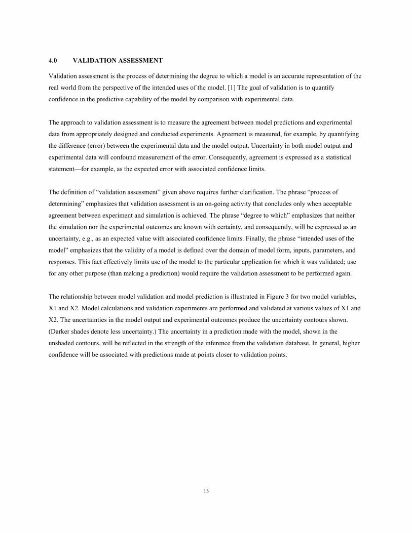
The relationship between model validation and model prediction is illustrated in Figure 3 for two model variables,

X1 and X2. Model calculations and validation experiments are performed and validated at various values of X1 and

X2. The uncertainties in the model output and experimental outcomes produce the uncertainty contours shown.

(Darker shades denote less uncertainty.) The uncertainty in a prediction made with the model, shown in the

unshaded contours, will be reflected in the strength of the inference from the validation database. In general, higher

confidence will be associated with predictions made at points closer to validation points.

14

Design Variable, X1

Des

ign

Varia

ble,

X2

Validation Points

Prediction Point

Design Variable, X1

Des

ign

Varia

ble,

X2

Validation Points

Prediction Point

Figure 3: Validation and application domain for two design variables.

It is important to emphasize that adjusting the model–either the model parameters or the basic equations–to improve

agreement between the model output and experimental measurements does not constitute validation. In some

instances, calibration (or model updating) is a useful activity; however it is part of the model-building process and

not the validation-assessment process. Moreover, it is often tempting to adjust the parameters of highly sophisticated

computer models to improve agreement with experimental results. This temptation is avoided if the model and

experimental results are kept separate until the comparisons are made.

4.1 Validation Hierarchy

Ultimately, the reality of interest shown in Figure 2 is a complete system. However, most systems comprise

multiple, complicated subsystems and components, each of which must be modeled and validated. The current state

of practice often attempts to validate system models directly from test data taken on the entire system. This approach

can be problematic if there are a large number of components or if subsystem models contain complex connections

or interfaces, energy dissipation mechanisms, or highly nonlinear behavior, for example. If there is poor agreement

between the prediction and the experiment, it can be difficult if not impossible to isolate which subsystem is

responsible for the discrepancy. Even if good agreement between prediction and experiment is observed, it is still

possible that the model quality could be poor because of error cancellation among the subsystem models. Therefore,

a strategy must be developed to conduct a sequence of experiments that builds confidence in the model's ability to

produce reliable simulations of system performance.

15

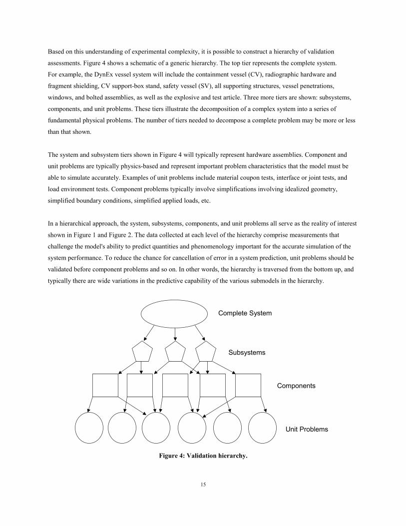
Based on this understanding of experimental complexity, it is possible to construct a hierarchy of validation

assessments. Figure 4 shows a schematic of a generic hierarchy. The top tier represents the complete system.

For example, the DynEx vessel system will include the containment vessel (CV), radiographic hardware and

fragment shielding, CV support-box stand, safety vessel (SV), all supporting structures, vessel penetrations,

windows, and bolted assemblies, as well as the explosive and test article. Three more tiers are shown: subsystems,

components, and unit problems. These tiers illustrate the decomposition of a complex system into a series of

fundamental physical problems. The number of tiers needed to decompose a complete problem may be more or less

than that shown.

The system and subsystem tiers shown in Figure 4 will typically represent hardware assemblies. Component and

unit problems are typically physics-based and represent important problem characteristics that the model must be

able to simulate accurately. Examples of unit problems include material coupon tests, interface or joint tests, and

load environment tests. Component problems typically involve simplifications involving idealized geometry,

simplified boundary conditions, simplified applied loads, etc.

In a hierarchical approach, the system, subsystems, components, and unit problems all serve as the reality of interest

shown in Figure 1 and Figure 2. The data collected at each level of the hierarchy comprise measurements that

challenge the model's ability to predict quantities and phenomenology important for the accurate simulation of the

system performance. To reduce the chance for cancellation of error in a system prediction, unit problems should be

validated before component problems and so on. In other words, the hierarchy is traversed from the bottom up, and

typically there are wide variations in the predictive capability of the various submodels in the hierarchy.

Complete System

Subsystems

Components

Unit Problems

Figure 4: Validation hierarchy.

16

Schedule or budget constraints may prohibit experiments needed to validate a model for every unit problem,

component, and subsystem defined in the validation hierarchy. In this situation, it can be useful to perform a

sensitivity analysis of the full-system model and identify the important problem characteristics that require more

careful definition and perhaps higher fidelity. This approach focuses the validation effort on only the physics that

contributes significantly to the response of interest. Another approach is to rely on expert judgment to estimate

uncertainties associated with elements of the hierarchy for which there are no data and to propagate these

uncertainties to the top level. The danger of these approaches lies in the use of the as yet unvalidated model or

incomplete information to determine, perhaps incorrectly, the important problem characteristics.

Careful construction of a validation hierarchy is of paramount importance because it defines the problem

characteristics that the model must be able to simulate, the coupling and interactions between unit problems, and the

complete system (denoted by the arrows in Figure 4), and, arguably most importantly, the validation experiments

that must be performed to validate the unit, components, and subsystem models. As an example, the DynEx vessel

must be designed to withstand the penetration and possible perforation of the vessel wall due to fragment impact.

This fact suggests several unit problems, such as the high-strain-rate inelastic behavior of the vessel wall, the

aluminum and beryllium material, and the structural response of the vessel wall impacted by fragments. Each of

these unit problems would serve as the “reality of interest” in Figure 2, and consequently, each model is constructed

and validated before assembling into components and repeating the process.

4.2 Validation Metrics

Complex model simulations generate an enormous amount of information from which to choose. The selection of

the simulation outcome should first be driven by application requirements. For example, if a design requirement is

that the peak strain at specified location should not exceed some value, then the model validation should focus on

comparison of measured and computed strains at that location.

Features of experimental data and model outputs must be carefully selected. A feature may be simple, such as the

maximum response for all times at a specific location in the computational domain, or more complex, such as the

complete response history at a specific location, modal frequencies, mode shapes, load-deflection curve slopes and

inflection points, peak amplitudes, signal decay rates, temporal moments, shock response spectra, etc. In some cases,

a feature can be used directly as a validation metric; in other cases, the feature must be processed further into a form

more suitable for comparison with experimental data.

17

A validation metric is the basis for comparing features from experimental data with model predictions. [13]

Validation metrics are established during the requirements phase of the conceptual model development and

incorporate numerical and experimental uncertainty. If the error, e , between experimental data, y , and model

prediction, *y , is given by *yye −= , a simple metric could be the expected value of the error, ( )eE , or the

variance of the error, ( )eV . Other metrics could include, for example: ( )0>eP , where ( )⋅P is the probability; the

95th percentiles on the probability distribution of e ; or a hypothesis test such as ( )0>eE , where the validation

metric is a pass/fail decision of whether or not the model is contradicted by the data.

Validation metrics must be established during the validation requirement phase of the conceptual model

development and should include estimates of the numerical and experimental error. In selecting the validation

metric, the primary consideration should be what the model must predict in conjunction with what types of data

could be available from the experiment. Additionally, the metrics should provide a measure of agreement that

includes uncertainty requirements.

4.3 Validation Experiments

Traditional experiments are performed to improve fundamental understanding of physical behavior, improve

mathematical models, estimate values of model parameters, and assess component or system performance. Data

from traditional experiments are generally inadequate for purposes of model validation because of lack of control or

documentation of some experimental parameters or inadequate measurement of specimen response. Generally, data

from the archive literature are from traditional experiments and do not meet the requirement of validation testing.

Therefore, for model V&V, it will usually be necessary to perform experiments dedicated to model validation.

In contrast to traditional experiments, validation experiments are performed to generate high-quality data for the

purpose of assessing the accuracy of a model prediction. A validation test is a physical realization of an initial-

boundary value problem. To qualify as a validation test, the specimen geometry, initial conditions, boundary

conditions, and all other model input parameters must be prescribed accurately. The response of the test specimen to

the loading must be measured with high, quantified accuracy. Data collected during the test should include the

applied loads as well as initial conditions and boundary conditions that might change throughout the test. In

addition, all prescribed input, test conditions, and measurements must be fully documented. Ideally, this approach

provides as many constraints as possible, requiring few, if any, assumptions on the part of the modeler.

The experimental data comprise the standard against which the model outputs are compared. Therefore, it is

essential to determine the accuracy and precision of the data from experiments. Uncertainty in the measured

quantities should be estimated so that the predictions from the model can be credibly assessed. Uncertainty and error

in experimental data include variability in test fixtures, installations, environmental conditions, and measurements.

Sources of nondeterminism in as-built systems and structures include design tolerances, residual stresses imposed

during construction, and different methods of construction.

18

In experimental work, errors are usually classified as being either random error (precision) or systematic error (bias).

An error is classified as random if it contributes to the scatter of the data in repeat experiments at the same facility.

Random errors are inherent to the experiment, produce nondeterministic effects, and cannot be reduced with

additional testing. Systematic errors produce reproducible or deterministic bias that can be reduced, although it is

difficult in most situations. Sources of systematic error include transducer calibration error, data acquisition error,

data reduction error, and test technique error.[14]

While not strictly necessary, agreement between experiment and simulation for other variables or at other locations

in the model adds qualitatively to the overall confidence placed in the model. Therefore, validation tests should

produce a variety of data so that many aspects of the model can be assessed. This assessment is important because,

although some quantities may be of secondary importance, accurate predictions of these quantities provide evidence

that the model accurately predicts the primary response for the right reason. This evidence qualitatively builds

confidence that the model can be used to make accurate predictions for problem specifications that are different

from those included in model development and validation.

Coordination with Modelers

Modelers should have input to the design of the validation tests. What is simple for an experimenter to measure may

not be simple for a modeler to predict, and vice versa. There must be a shared understanding of what responses are

difficult to measure or predict. Additionally, the modelers must be certain that all inputs (especially for constitutive

models), boundary conditions, and imposed loads are being measured. The need for collaboration should not be

overlooked.

Modelers should perform a parametric study with the verified model to determine model sensitivities that must be

investigated experimentally. Additionally, pretest analyses should be conducted to uncover potential problems with

the experiment design.

Finally, it is highly advisable that the model developer not know the test results before the model prediction is

complete. Exceptions, of course, are the measured load and boundary conditions, if applicable. Because many

problems show significant sensitivity to physical and numerical parameters, it is often tempting to adjust the

prediction of highly sophisticated computer models to match measurements. This course of action must be avoided,

however, because it does not constitute validation.

Measurement Requirements

Measurements must have known accuracy and precision, which must be established through calibration of the

transducers and documentation of inaccuracies related to nonlinearity, repeatability, and hysteresis. Uncertainty in

measurement accuracy is rarely quoted. However, it is necessary to estimate the uncertainty in the measurements so

that model predictions can be judged appropriately.

19

Many sources can affect a gauge output. Transducers should be calibrated in an environment similar to that of the

test, e.g., at elevated temperature. If a transducer is sensitive to the environment, and the environment changes

significantly during the test, the transducer sensitivity to the environment must be established so that the resulting

data can be corrected to account for the sensitivity to environment. The compliance or inertia of any test fixtures

must be determined and accounted for if they contribute to the measurement of displacement or force, respectively.

Additional tests dedicated to demonstrating the accuracy of the measurements have been shown to be very helpful.

Redundant measurements are needed to establish the variability (scatter) in the test results. This establishment of

variability can be accomplished, for example, by repeating tests on different specimens. If the cost of testing is high

or the availability of test specimens is limited, redundant measurements obtained by placing similar transducers at

symmetrical locations (if the test has adequate symmetry) can also assess scatter. The data from these transducers

can also be used to determine if the desired symmetry was indeed obtained. Consistency of the data is an important

attribute of the test that increases confidence in the test data. Data consistency can be established by independent or

corroborative measurements, e.g., stress and velocity, as well as by measurements of point quantities made in

families so that fields can be estimated.

There are two basic approaches to experimental error estimation: 1) estimation and characterization of all the

elemental uncertainties that combine to produce the total experimental error, and 2) the use of replicate testing to

provide direct statistical estimates of the total experimental uncertainty. The former approach is attractive in that it

provides a means of error source identification but requires data from independent sources or a large amount of

supplementary testing. In practice, some combination of the two approaches can be used. For this reason,

well-thought-out validation test programs usually provide for an appropriate amount of experimental replication.

4.4 Uncertainty Quantification

It is widely understood and accepted that uncertainties, whether reducible (random) or irreducible (systematic), arise

because of the inherent randomness in physical systems, modeling idealizations, experimental variability,

measurement inaccuracy, etc., and cannot be ignored. This fact complicates the already difficult process of model

validation by creating an unsure target—a situation in which neither the simulated nor the observed behavior of the

system is known with certainty.

Nondeterminism refers to the existence of errors and uncertainties in the outputs of computational simulations

because of inherent and/or subjective uncertainties in the model inputs or model form. Likewise, the measurements

that are made to validate these simulation outcomes also contain errors and uncertainties. In fact, it is important to

note that while the experimental outcome is used as the reference, the V&V process does not presume the

experiment to be more accurate than the simulation. Instead, the goal is to quantify the uncertainties in both

experimental and simulation results such that the model requirements can be assessed (validation) and the predictive

accuracy of the model quantified.

20

Uncertainty and error can be categorized as error, irreducible uncertainty, and reducible uncertainty. Errors create a

reproducible (i.e. deterministic) bias in the prediction and can theoretically be reduced or eliminated. Errors can be

acknowledged (detected) or unacknowledged (undetected). Examples include inaccurate model form,

implementation errors in the computational code, nonconverged computational models, etc.

“Irreducible uncertainty” (i.e., variability, inherent uncertainty, aleatory uncertainty) refers to the inherent variations

in the system that is being modeled. This type of uncertainty always exists in physical systems and is an inherent

property of the system. Examples include variations in system geometric or material properties, loading

environment, assembly procedures, etc.

“Reducible uncertainty” (i.e., epistemic uncertainty) refers to deficiencies that result from a lack of complete

information about the system being modeled. An example of reducible uncertainty is the statistical distribution of a

geometric property of a population of parts. Measurements on a small number of the parts will allow estimation of a

mean and standard deviation for this distribution. However, unless this sample size is sufficiently large (i.e.,

infinite), there will be uncertainty about the “true” values of these statistics, and, indeed, uncertainty regarding the

“true” shape of the distribution. Obtaining more information (in this case, more sample parts to measure) will allow

reduction of this uncertainty and a better estimate of the true distribution.

Nondeterminism is generally modeled through the theory of probability. The two dominant approaches to

probability are the frequentist approach in which probability is defined as the number of occurrences of an event,

and the Bayesian approach, in which probability is defined as the subjective opinion of the analyst about an event.

Other mathematical theories have also been developed for representing uncertainty, such as fuzzy sets, evidence

(Dempster-Shafer) theory, the theory of random sets, and the theory of information gap; however, their application

to computationally-intensive problems is less well-developed than probabilistic methods.

Much of the nondeterministic information that exists in a numerical model can be identified and treated in order to

quantify its effects and in some cases even reduce these effects. The first class of information is the uncertainty

associated with the model input parameters such as material behavior, geometry, load environment, initial

conditions, or boundary conditions. The variability (irreducible uncertainty) of these parameters can be estimated

using repeated experiments to establish a statistically significant sample. In lieu of sufficient data, expert opinion

may be elicited to estimate distribution parameters or bounds; however, the imprecise nature of expert opinion must

be reflected as additional uncertainty in the simulation outcomes.

When the variability in the model input parameters has been established, this variability can be propagated through

the simulation to establish an expected variability on the simulation output quantities. Sampling-based propagation

methods (Monte Carlo, Latin Hypercube, etc.) are straightforward, albeit inefficient, techniques for propagating

variabilities. These methods draw samples from the input parameter populations, evaluate the deterministic model

21

using these samples, and then build a distribution of the appropriate response quantities. Sampling methods can be

made more efficient by the use of local response surface approximations (e.g., metamodel, reduced-order model,

etc.) of the model being studied. However, the error involved in the use of a response surface must also be

estimated. Sensitivity-based methods that are more efficient than sampling-based methods may also be used to

propagate input uncertainties to uncertainties on the response quantities. Well known sensitivity-based methods

include the First Order Reliability Methods (FORM), Advanced Mean Value (AMV), and Adaptive Importance

Sampling (AIS).

When little or no direct evidence is available for uncertainty quantification of the models and experiments, an

alternative uncertainty characterization based on a generic class of model-test pairs may be useful. This approach

estimates uncertainty based on the statistics of the differences between models and experiments that are generically

similar to the problem at hand. However, the interpretation of such an analysis can be difficult and depends on the

definition of the generic class and the constituents of that class.

4.5 Validation Requirements and Acceptable Agreement

The final step in the validation process is to compare values of the metrics chosen to measure the agreement between

model outputs with the experimental data and to make an assessment of model accuracy. The determination of

whether or not the validated system-level model is adequate for its intended use is a programmatic decision and

involves both technical and nontechnical requirements such as schedule, availability, financial resources, public

perception, etc. Stakeholders who are not part of the validation team will typically determine these nontechnical

requirements. Therefore, the interpretation of adequacy is limited here to include only the acceptable agreement

between experimental and simulation outcomes.

In Figure 4, the system-level model accuracy goal is used to establish accuracy requirements for each subordinate

model in the validation hierarchy. These requirements should be established such that the unit, component, and

subsystem models are developed at least to the degree of fidelity required to meet the system-model accuracy goal.

A sensitivity analysis of the complete system can be used to identify the importance/contribution of each model,

which can then be used to establish commensurate accuracy requirements.

The required accuracy between simulation and experimental outcomes should be established before the comparison

is made. It is reasonable to expect that the accuracy objective for unit problems will be more stringent than for the

complete system because of the simpler nature of unit problems. For example, a 2% accuracy expectation might be

established for a unit model that predicts the axial deformation of a bolt in tension, whereas the accuracy expectation

might be 5% or more for a model that predicts the dynamic response of the bolt under combined loadings. For

example, an accuracy requirement might be expressed in a statement such as, “A model is desired that is accurate to

within 10% with 95% confidence.”

22

5.0 MODEL AND EXPERIMENT REVISION

If the agreement between experimental and simulation outcomes is unacceptable, the model and/or experiment may

need to undergo revisions. These revisions should reflect knowledge about the mechanics of the system that was

gained during the process of comparing the experimental and simulation outcomes. The revisions should also reflect

further knowledge that has been obtained regarding the behavior of the constituent materials, initial conditions, or

boundary conditions. The revisions may reflect new knowledge about the characteristics of the applied loads that

will affect the output of the simulation model. In a general sense, revisions to the model can be divided into two

broad classes: revisions to the parameters of the mathematical/computational model, and revisions to the form of the

conceptual model itself.

The ad hoc adjustment of model parameters to bring the model into better agreement with experimental outcomes is

strongly discouraged. In some references, this practice has been termed “model calibration.” Model calibration

should not be confused with a “calibration experiment,” which is an experiment performed to determine values for

constitutive model parameters. While model calibration may produce better agreement between the experiment and

the model, the predictive capability of the model will be compromised by the introduction of additional empirical

calibration factors (because the the model may produce the right answer for the wrong reason).

When model revision is required to improve the agreement between simulation and experiment, two techniques can

be used to estimate revised values of the parameters in the model: 1) parametric model calibration, and

2) independent measurements of the parameter values.

Revision by parametric model calibration is extensively used in the field of linear structural dynamics to bring

computational predictions into better agreement with measured response quantities. Terms such as “model

updating,” “parameter calibration,” and “parameter estimation” are commonly used to describe such a technique.

While the revision of model parameters in this way can be a scientifically legitimate method of improving the

predictive accuracy of a structural dynamics model, care must be exercised to ensure that it is not done in an ad hoc

manner. In the performance of parameter calibration, optimization techniques (such as least squares fitting) are

commonly employed to estimate the values of model parameters such that the value of an objective function is

minimized. Finally, a model that has been calibrated must be revalidated.

Parameter calibration is commonly used to “tune” the performance of a linear vibration model so that the measured

modal quantities (e.g., modal frequencies and mode shapes) of the simulation are brought into agreement with the

corresponding parameters obtained in measurements. The most common sources of model difficulties in structural

dynamics—compliance in joints, energy loss/damping, unmeasured excitations, uncertain initial and boundary

conditions—can thus be represented as simple mechanical models and the submodel parameters calibrated so that

the global response is in agreement.

23

The second approach for parametric model revision is to isolate the parameters of interest and make an independent

measurement of the responses. Once additional information is obtained on these parameters, the model may be

updated with new parameter values.

The second class of model revisions that can be made involves changes to the form of the conceptual model, which

may or may not require changes in the mathematical and computational model. Typically, this type of change will

be a result of observations made during the experimental phase and/or validation assessment phase in which some

characteristics in the response of the structure are not consistent with the corresponding characteristics of the

simulation model output and the differences are not attributable to reasonable inaccuracies in the model parameters.

There are many common types of deficiencies in model form that can be responsible for inaccurate simulation

results: two-dimensional models that cannot represent three-dimensional response effects; the wrong model form for

elastic or plastic response of a material; assumptions about contact being tied when in reality a gap develops

between two parts; assumptions that two parts do not move relative to one another when in reality they do and

significant friction forces are developed; rigid boundary conditions that turn out to have significant compliance, etc.

It is important to look for possible violation of the assumptions of the model form when reconciling the measured

data with the results of the computational simulation. Should the equations or model parameters change, the process

of model verification and validation must be performed again. Moreover, if parameters were changed using data

from some or all of the validation experiments, then new experiments must be performed to provide evidence for the

validation.

24

6.0 SUMMARY AND CONCLUSIONS

This report has presented the concepts of Model Verification and Validation (V&V). The scope of the report

includes the philosophy, general concepts, and processes for conducting a successful V&V program. While the

LANL DynEx Vessel Program motivated the development of this report, the concepts presented are general and

applicable to any program requiring the use of validated numerical models. In a subsequent report, specific V&V

procedures required to implement these concepts and to make recommendations for the DynEx vessel design and

analysis will be developed.

There are many open issues in the definition and practice of V&V. From a practical standpoint, the costs associated

with conducting a high quality V&V program could be formidable. Therefore, the long-term benefits of using a

validated model to supplement physical testing must be balanced against the costs associated with model

development and model V&V. The resource requirements associated with model V&V necessitate a graded

approach to the application of V&V requirements.

The need to reduce time and costs associated with large-scale physical testing drive the reliance on modeling and

simulation upward in the field of computational mechanics. This fact, in turn, motivates the continued development

of methodology and tools for performing model V&V. Several areas in which further research and development are

needed have been identified:

• peer-reviewed and accepted procedures for developing a validated model;

• methods and tools for performing uncertainty quantification considering both inherent and epistemic

uncertainty;

• methodology for establishing a validation hierarchy and associated model-validation requirements;

• Validation metrics, performance measures, and computational features to support validation

comparisons; and

• ways of computing error and confidence via statistical analysis of computational and simulation

outcomes, and methods for identifying optimal model revision strategies via sensitivity analysis.

25

ACKNOWLEDGMENTS

The author gratefully acknowledges the following individuals for their input and time spent discussing the

concepts presented in this report: Drs. Mark Anderson, Scott Doebling, and François Hemez, Mr. Jason Pepin,

and Edward A. Rodriguez, all of Los Alamos National Laboratory; Dr. Leonard Schwer of Schwer Engineering

& Consulting Services, chairman of ASME Committee #60, Verification and Validation in Computational Solid

Mechanics; and Dr. Paul Senseny of FM Global Research. The author also appreciates the interactions with other

ASME Committee #60 members that occurred during the development of this report.

26

27

REFERENCES

(1) American Institute of Aeronautics and Astronautics, Guide for the Verification and Validation of

Computational Fluid Dynamics Simulations, AIAA-G-077-1998, Reston, VA, 1998.

(2) Los Alamos National Laboratory, Quality Assurance Plan, DynEx Vessel Project, DV-QAP, Rev. 1,

July 15, 2002.

(3) American Society of Mechanical Engineers, Council on Codes and Standards, Board on Performance Test

Codes #60, Committee on Verification and Validation in Computational Solid Mechanics,

http://www.asme.org/cns/departments/performance/ public/ptc60/.

(4) United States Department of Defense, Defense Modeling and Simulation Office (DMSO), “Verification,

Validation, and Accreditation,” https://www.dmso.mil/public/ transition/vva/.

(5) Advanced Simulation and Computing V&V Strategy and Plan, Los Alamos National Laboratory,

Version 2.2 (Draft), LA-UR-02-4314, July 2002.

(6) Oberkampf, W.L., S.M. DeLand, et al., “Estimation of Total Uncertainty in Modeling and Simulation,”

Sandia National Laboratories, SAND2000-0824, April 2000.

(7) Logan, R.L., and C.K. Nitta, “Verification & Validation (V&V) Guidelines and Quantitative Reliability at

Confidence (QRC): Basis for an Investment Strategy,” Lawrence Livermore National Laboratory,

UCRL-2002x0266 (Draft), August 2002.

(8) Schlesinger, S., “Terminology for Model Credibility,” Simulation, Vol. 32, No. 3, 1979.

(9) Roach, P.J., Verification and Validation in Computational Science and Engineering, Hermosa Publishers,

Albuquerque, NM, 1998.

(10) Salari, K., and P. Knupp, “Code Verification by the Method of Manufactured Solutions,” Sandia National

Laboratories, SAND2000-1444, June, 2000.

(11) Oberkampf, W.L., T.G. Trucano, and C. Hirsch, “Verification, Validation, and Predictive Capability in

Computational Engineering and Physics,” SAND2003-3769, February, 2003.

(12) Thacker, B.H., D.S. Riha, H.R. Millwater, and M.P. Enright, “Errors and Uncertainties in Probabilistic

Engineering Analysis,” Proc. 42nd AIAA/ASME/ASCE/AHS/ASC Structures, Structural Dynamics, and

Materials Conference and Exhibit, Seattle, Washington, 2001.

(13) Trucano, T.G., R.G. Easterling, K.J. Dowding, et al., “Description of the Sandia Validation Metrics

Project,” SAND2001-1339, July 2001.

(14) Coleman, H.W., W.G. Steele, Jr., “Experimentation and Uncertainty Analysis for Engineers,” John Wiley

& Sons, 1989.

This report has been reproduced directly from thebest available copy. It is available electronicallyon the Web (http://www.doe.gov/bridge).

Copies are available for sale to U.S. Departmentof Energy employees and contractors from:

Office of Scientific and Technical InformationP.O. Box 62Oak Ridge, TN 37831(865) 576-8401

Copies are available for sale to the public from:National Technical Information ServiceU.S. Department of Commerce5285 Port Royal RoadSpringfield, VA 22161(800) 553-6847