cutting parameters optimisation in milling: expert

Int. J. Mechatronics and Manufacturing Systems, Vol. x, No. x, xxxx 1

Cutting Parameters Optimisation in Milling: ExpertMachinist Knowledge versus Soft Computing Methods

J.V. Abellan-NebotDepartment of Industrial Systems Engineering and Design,School of Technology and Experimental Sciences, Universitat Jaume I,12071 Castellon, SpainFax: +34964728170 E-mail: [email protected]

AbstractIn traditional machining operations, cutting parameters are usually selected

prior to machining according to machining handbooks and user’s experience.However, this method tends to be conservative and sub-optimal since part ac-curacy and non machining failures prevail over machining process efficiency. Inthis paper, a comparison between traditional cutting parameter optimisation by anexpert machinist and an experimental optimisation procedure based on Soft Com-puting methods is conducted. The optimisation procedure presented is composedof two steps: (1) modelling the process variables of interest and (2) optimising amulti-objective function to reach a trade-off among production rate, cutting costsand part accuracy. The first step applies an Adaptive Neuro-fuzzy Inference Sys-tem (ANFIS) to model the process by extracting rules from experimental data.The second step applies Genetic Algorithms to optimise the multi-objective func-tion which is defined by an overall desirability function approach. The proposedmethodology increased the machining performance in 6.1% and improved theunderstanding of the machining operation through the ANFIS models.

Keywords: Machining, Parameters Optimisation, Adaptive Neuro-Fuzzy Infer-ence Systems, Soft Computing, Genetic Algorithms, Multi-Objective Functions,Expert Machinist, Desirability Functions.

Reference to this paper should be made as follows:

Biographical Notes: Jose V. Abellan-Nebot is assistant professor in the De-partment of Industrial Systems Engineering and Design at Jaume I University.He received the M.Sc. degree in manufacturing engineering in 2003. In 2004, hejoined the Department as a research assistant. Since 2007, he lecturers ComputerIntegrated Manufacturing, Computer Aided Manufacturing and ManufacturingTechnologies. He was a visiting scholar at the Centre for Innovation in Designand Technology located at Monterrey Institute of Technology (Mexico) in 2005and at the Engineering Research Center for Reconfigurable Manufacturing Sys-tems (ERC-RMS) at University of Michigan in 2007. He is author of more thanfifteen conference proceedings and several research studies published at interna-tional journals. His research interests include issues related to intelligent machin-ing systems, stream of variation in machining systems and manufacturing andcollaborative engineering.

Post-print. Author’s version. Universitat Jaume I

Repositori institucional UJI

2 J.V. Abellan-Nebot

1 Introduction

Metal cutting is one of the important and widely used manufacturing processes in en-gineering industries. The study of metal cutting focuses, among others, on the features oftools, input work materials, and machine parameter settings influencing machining processefficiency and output quality characteristics. A significant improvement in machining pro-cess efficiency may be obtained by process parameter optimisation that identifies and deter-mines the regions of critical process control factors leading to desired outputs or responseswith lower manufacturing cost (Mukherjee and Ray, 2006). However, in traditional Com-puter Numerical Control (CNC) systems machining parameters are usually selected prior tomachining according to machining handbooks or user’s experience, which is a conservativeand sub-optimal procedure to assure part quality specifications without machining failure.

In order to overcome the limitations of traditional cutting parameter selection, exper-imental process parameter optimisation procedures should be applied in industry. Theseprocedures are composed of two steps: (1) modelling of process variables relationshipthrough experimentation, and (2) determination of optimal or near-optimal cutting con-ditions through optimisation algorithms. First step deals with representing the machiningprocess through mathematical models required for a later formulation of the process ob-jective function. In the literature, several modelling techniques have been implementedmainly based on statistical regressions (Cus and Balic, 2003), artificial neural networks(Liu and Wang, 1999a; Chiang et al., 1995; Liu et al., 1999b; Zuperl and Cus, 2003; Chienand Chou, 2001) and fuzzy set theory (Ip, Lau and Chan, 2003). Second step providesoptimal or near-optimal solution(s) to the overall optimisation problem formulated throughthe previous mathematical models. In the literature, the main optimisation tools and tech-niques applied are based on Taguchi method (Ghani, Choudhury and Hassan, 2004; Zhang,Chen and Kirby, 2007), response surface design (Suresh, Rao and Deshmukh, 2002), ge-netic algorithms (Liu, Zuo and Wang, 1999b; Suresh, Rao and Deshmukh, 2002; Cus andBalic, 2003; Chien and Chou, 2001) and simulated annealing (Juan, Yu and Lee, 2003).

Cutting parameter optimisation in machining has been intensively studied in the liter-ature as it can be stated in a recent review (Mukherjee and Ray, 2006). Liu and Wang(1999a) proposed an adaptive control system based on two neural network models, a Back-Propagation Neural Networks (BP NN) and an Augmented Lagrange Multiplier NeuralNetwork (ALM NN). The BP NN was used for modelling the state of the milling system,using as a single input the feed parameter and sensing the cutting forces on-line. The ALMNN was used for maximising the material removal rate which it was carried out adjustingthe feed rate. Chiang et al. (1995) presented a similar work for end-milling operations,but surface roughness was also considered as constraint. Both research works were basedon theoretical formulas for training the neural networks and both applied an ALM NN foroptimisation. Liu, Zuo and Wang (1999b) also extended his previous work with a newoptimisation procedure based on a Genetic Algorithm (GA). Ghani, Choudhury and Has-san (2004) optimised cutting parameters using a Taguchi’s Design of Experiments in endmilling operations. With a minimum number of trials compared with other approaches suchas a full factorial design, the methodology presented reveals the most significant factors andinteractions during cutting process which leads to choose the optimal conditions. A verysimilar methodology was described by Zhang, Chen and Kirby (2007). However, bothmethodologies do not permit to evaluate quadratic or non-linear relations between factors,


Cutting Parameters Optimisation in Milling: Machinist Knowledge vs Soft Computing 3

and the analysis is restricted to the levels analysed in each factor. A more generic ap-proach although more costly in experiments is based on Response Surface Model optimisa-tion (RSMO). Suresh, Rao and Deshmukh (2002) used the Response Surface Methodology(RSM) for modelling the surface roughness as a first and second-ordermathematical model.The surface roughness optimisation was carried out through GA which are time consumingand are more appropriate for optimising non-linear functions. Cus and Balic (2003) alsoapplied GA for optimising a multi-objective function based on minimum time necessaryfor manufacturing, minimum unit cost and minimum surface roughness. All the processmodels applied in their research were empirical formulaes from machining handbooks andthey were adjusted through regressions. More complex models have been also applied forsurface roughness and tool wear modelling to optimise off-line cutting parameters. Zuperland Cus (2003) also applied and compared feed-forward and radial basis neural networksfor learning a multi-objective function similar to the one presented by Cus and Balic (2003).Choosing the radial basis networks due to their fast learning ability and reliability, they ap-plied a large-scale optimisation algorithm to obtain the optimal cutting parameters. Chienand Chou (2001) applied neural networks for modelling surface roughness, cutting forcesand cutting-tool life and applied a GA to find optimum cutting conditions for maximisingthe material removal rate under the constraints of the expected surface roughness and toollife. Ip, Lau and Chan (2003) applied fuzzy sets to optimise the material removal rate inthe manufacturing of sculptured surfaces and they demonstrated a material removal rate in-crease of 41% in comparison with conventional constant feedrate. Juan, Yu and Lee (2003)applied polynomial networks to model a roughing milling operation, and the productioncost was minimised using a simulated annealing method. Table 1 summaries recent re-search works related to cutting parameter optimisation.

Table 1 Literature review on cutting parameter optimisation.Modelling Optimisation Output

Reference Approach Approach Optimised Process(Liu and Wang, 1999a) Feed-forward NN ALM NN MRR M(Chiang et al., 1995) Feed-forward NN ALM NN MRR EM(Liu et al., 1999b) Feed-forward NN GA MRR M(Ghani et al., 2004) — TA CF, Ra EM(Zhang et al., 2007) — TA Ra EM(Suresh et al., 2002) Response Surface GA Ra T(Cus and Balic, 2003) Statistical Regressions GA Unit cost, Ra T

Time(Zuperl and Cus, 2003) Feed-forward and LSO MRR, Tl T

Radial Basis NN Ra(Chien and Chou, 2001) Feed-forward NN GA MRR T(Ip et al., 2003) Fuzzy Sets — MRR M(Juan et al., 2003) Polynomial Networks SA Production cost MMRR:Material Removal Rate; Tl: Tool-life; Ra: Surface Roughness; CF: Cutting Force;GA: Genetic Algorithm; TA: Taguchi Approach; ALM NN: Augmented Lagrange Multiplier;LSO: Large Scale Optimisation; SA: Simulated AnnealingT: Turning; EM: End Milling;M:Milling;

In this paper, the traditional optimisation procedure based on machinist’s expertise iscompared with an experimental cutting optimisation procedure based on Soft Computingmethods. The Soft Computing methods applied to model the process is the Adaptive Neuro-Fuzzy Inference System (ANFIS), which describes the process knowledge in a form of If-



Then rules. Unlike other methods presented in the literature such as Neural Networks (NN),Fuzzy, Response Surface (see Table 1), ANFIS models let understand the process throughsimple rules extracted from experimental data, so the expert machinist is able to learn newknowledge from a particular machining operation and confirmwell-knownmachining prac-tices/rules. The comparison is conducted in a finishing face-milling operation with CubicBoron Nitride (CBN) cutting tools, which are modern and expensive cutting tools. Thecutting parameter optimisation deals with a multi-objective function where surface rough-ness, tool life, material removal rate and quality loss functions are considered through adesirability function approach. The final optimisation algorithm is based on another softcomputing method called Genetic Algorithm (GA).

2 Machining Process Description

The machining process studied in this paper is presented in Figure 1, and it consists of aface-milling operation on workpieces of hardened AISID3 steel (60HRc) with dimensions250 × 250 mm. The experiments were conducted on a CNC machining centre suited formould and die manufacturing, and the cutting tool used was a face milling tool with CubicBoron Nitride (CBN) inserts. In order to generate a good surface finish and avoid run-outproblems, a single insert was mounted on a tool body with an effective diameter of 40 mm.

Figure 1 Machining process analysed: face-milling operation on workpieces of hardened AISID3 steel (60 HRc) with dimensions 250 × 250 mm and Cubic Boron Nitride (CBN) cutting inserts.

3 Definition of the Optimisation Problem

3.1 Objective Functions

Typically, three objective functions are considered in a cutting parameters optimisationproblem: material removal rate, surface roughness and cutting-tool life. Material RemovalRate (MRR) is a measurement of productivity, and it can be expressed by equation (1),



where Vc, fz and ap are the cutting speed, feed rate per tooth and depth of cut respectively.Most of the cutting parameter optimisation procedures in roughing operations try to max-imiseMRR constrained to cutting forces (Liu and Wang, 1999a). Surface roughness (Ra)is the most important criterion for the assessment of the surface quality, and it is usually cal-culated empirically through experiments. Surface roughness can be described as an empiri-cal relationship among the cutting parameters Vc, fz , ap, and it is commonly minimised forhigh quality machining operations (Zhang, Chen and Kirby, 2007; Suresh, Rao and Desh-mukh, 2002). Cutting-tool life (T ) is the other important criterion for cutting parametersselection, since several costs such as cutting-tool replacement cost and cutting-tool cost aredirectly related with cutting-tool life. The tool life can be also described as an empirical re-lationship among the cutting parameters Vc, fz , ap, and it is usually fixed to find a trade-offbetween cutting-tool/replacement costs and production rate (Cus and Balic, 2003; Zuperland Cus, 2003). In addition to these three objective functions, the Taguchi’s loss qualityfunction (W ) can be another important objective function for finishing operations since thesurface roughness variability along part surface impacts on the final part quality. Consider-ing a desired Ra value, the quality loss function is usually applied to estimate the cost ofmanufacturing with a quality variation. AsRa,W is commonly minimised for high qualitymachining operations. Therefore, the four objective functions which have to be taken intoconsideration for an optimal cutting parameter selection can be listed as follows:

(1) MRR = 1000Vcfzap

(2) Ra = f(Vc, fz, ap)

(3) T = f(Vc, fz, ap)

(4) W = AreworkV 2

∆2

where ∆ = Ramax − Ratarget. Ramax and Ratarget define the maximum Ra by partspecifications and the Ra desired respectively. V 2 defines the mean squared deviation asV 2 = ((Ratarget − y1)2 + + (Ratarget − yn)2)/n , with n the number of samples andArework is the part cost if the part is outside specifications. In several research works(Suresh, Rao and Deshmukh, 2002; Cus and Balic, 2003), the surface roughness and cuttingtool life functions have been described by well-known empirical equations as follows:

(5) Ra = kV x1fx2

z ax3

p

(6) T =KT

V α1fα2z aα3

p

where k, x1, x2, x3, KT , α1, α2, α3 are empirical coefficients. However, for high qualitymachining operations with CBN cutting tools, both equations may not provide a good esti-mation. The main reason is that additional mechanisms such as vibrations, engagement ofthe cutting tool or built up edge influence the surface roughness generationwhen machiningat very low feed speeds (Siller et al., 2008) . Furthermore, CBN tools have a different wearprocess than traditional cutting-tools such as high speed steels, so equation (6) may not bedirectly applied (Trent and Wright, 2000).



3.2 Multi-Objective Function

The optimisation problem for the case study is defined as the optimisation of a multi-objective function which is composed of the objective functions defined by Equations (1,2, 3 and 4). Due to these objective functions are conflicting and incomparable, the multi-objective function is defined using the desirability function approach. The desirability func-tion approach is based on the idea that the optimal performance of a process that has multi-ple performance characteristics is reached when the process operates under the most desir-able performance values (NIST/SEMATECH, 2006). For each objective function Yi(x), adesirability function di(Yi) assigns numbers between 0 and 1 to the possible values of Yi,with di(Yi) = 0 representing a completely undesirable value of Yi and di(Yi) = 1 repre-senting a completely desirable or ideal objective value. Depending on whether a particu-lar objective function Yi is to be maximised or minimised, different desirability functionsdi(Yi) can be used. A useful class of desirability functions was proposed by Derringer andSuich (1980). Let Li and Ui be the lower and upper values of the objective function respec-tively, with Li < Ui, and let Ti be the desired value for the objective function. Then, if anobjective function Yi(x) is to be maximised, the individual desirability function is definedas

(7) di(Yi) =

0 If Yi(x) < Li(

Yi−Li

Ti−Li

)wIf Li ! Yi(x) ! Ti

1 If Yi(x) > Ti

where the exponentw is a weighting factor which determines how important it is to hit thetarget value. For w = 1, the desirability function increases linearly towards Ti; for w < 1,the function is convex and there is less emphasis on the target; and for w > 1, the functionis concave and there is more emphasis on the target. If one wants to minimise an objectivefunction instead, the individual desirability is defined as

(8) di(Yi) =

1 If Yi(x) < Ti(

Yi−Ui

Ti−Ui

)wIf Ti ! Yi(x) ! Ui

0 If Yi(x) > Ui

Figure 2 shows the individual desirability functions according to different w values.The individual desirability functions are combined to defined the multi-objective function,called the overall desirability of the multi-objective function. This measure of compositedesirability is the weighted geometric mean of the individual desirabilities for the objectivefunctions. The optimal solution (optimal operating conditions) can then be determinedby maximising the composite desirability. The individual desirabilities are weighted byimportance factors Ii. Therefore, the multi-objective function or the overall desirabilityfunction to optimise is defined as:

(9) D = (d1(Y1)I1 × d2(Y2)

I2 × · · ·× dk(Yk)Ik)1/(I1+I2+···+Ik)

with k denoting the number of objective functions and Ii is the importance for the objectivefunction i (i = 1, 2, · · · , k).



Figure 2 Individual desirability functions for minimising or maximising objective functions. Theweighting factor determines how the desirability function increases/decreases.

3.3 Constraints

Due to the limitations on the cutting process, manufacturers limit the operation range ofcutting parameters to avoid premature cutting-tool failures. Therefore, the cutting parame-ter selection according to manufacturer specifications is constrained to:

(10) Vmin ! Vc ! Vmax fmin ! fz ! fmax ap ! amax

Surface roughness and quality loss specification are also considered as constraints thatcan be expressed as

(11) Ra ! Raspec W ! Wmax

In addition, cutting power and force limitations are usual constraints, but they are morecommonly applied in roughing operations.

3.4 Summary of Optimisation Problem and Numerical Coefficients

The weights and the individual desirability coefficients for each objective function werechosen according to machining process characteristics. First the weights were defined con-sidering how the objective function increases or decreases as the ideal value is not matched.In order to simplify the desirability functions, the weighting factor at each desirability func-tion was set to 1, so all desirability functions were defined as linear functions where thedesirability increases linearly towards the target value. Secondly, the coefficients of im-portance for each objective function were set according to machining requirements. Forthe case study, it was assumed that the machining process requires as first objective a highproduction rate (high MRR), a low cutting-tool costs (high T ) as a second objective, andas a third and less important objective a high part quality (low Ra and low W ). In orderto determine the overall desirability function (the multi-objective function), a numericalapproximation of the relative importance among individual objective functions is required.Although this estimation is subjective, it can be an easy and fast way to approximate thecutting parameter selection to the near-optimal one. For a more accurate definition of multi-objective functions it is required the definition of all machining costs, cutting-tools, labourcosts, product sale price, machine-tool operation cost, etc., which can be in some cases diffi-cult to know. For the case study, the coefficient of importance for each desirability functionwere set to 4, 1, 0.75, 0.75 for MRR, T , Ra and W respectively. Considering the maxi-mum and minimum value of each objective function obtained analytically, the desirabilityfunctions were defined as follows.



• MRR desirability function

(12) d1(MRR) =MRR − 390

2387− 390

MRRtarget = 2387 mm3/min. MRRminimum = 390 mm3/min. Importancefactor I1 = 4.

• Desirability function of Ra deviation objective function

(13) d2(W ) = d2(V2) =

V 2 − 0.013

0.0001 − 0.013

V 2target = 0.0001 µm2. V 2

maximum = 0.013 µm2. Importance factor I2 = 0.75.Note that the desirability function of quality loss W for surface roughness can bedefined by the surface roughness deviation V 2 since Equation (4) relatesW with V 2

by a constant coefficient of Arework/∆2.

• Ra desirability function

(14) d3(Ra) =Ra − 0.2

0.1 − 0.2

Ratarget = 0.1 µm. Ramaximum = 0.2 µm. Importance factor I3 = 0.75.

• Cutting-tool life desirability function.

(15) d4(T ) =T − 6

46.7 − 6

Ttarget = 46.7 min. Tminimum = 6 min. Importance factor I4 = 1.

The multi-objective function or the overall desirability function to be optimised is:

(16) D = (d1(MRR)4 × d2(V2)0.75

× d3(Ra)0.75× d4(T )1)1/(4+0.75+0.75+1)

constrained to:

(17) 100m/min ! Vc ! 200m/min 0.04mm/rev ! fz ! 0.12mm/rev

(18) ap = 4mm Ra ! 0.2µm V 2 ! 0.013µm2

4 Parameter Optimisation based on an Expert Machinist

4.1 Methodology

Cutting tool parameters are traditionally chosen according to handbooks, cutting-tooldata catalogs and machinist’s experience. For a given cutting-tool and workpiece material,a range of possible cutting-parameters are provided by the cutting-tool supplier, and themachinist chooses the parameters within the admissible operation ranges using some well-known practices in shop-floor. Some of these practices are:



Figure 3 Parameter optimisation based on an expert machinist knowledge. Knowing productspecifications and using handbooks and catalogs, the expert selects the optimal cutting parameters.

• Higher cutting speeds increase surface roughness quality but decrease cutting toollife.

• Higher cutting speeds decrease cutting tool life.

• Higher feed rates increase productivity as it is increased material removal rate.

• Higher feed rates decrease surface roughness quality.

• Higher feed rates decrease cutting-tool life.

• Higher axial depths of cut increase productivity.

• Higher axial depths of cut decrease cutting-tool life.

• Very low axial depths of cut burn the workpiece surface and generate a low surfaceroughness quality decreasing cutting-tool life.

According to the final goal of the machining process, the machinist selects the bestcutting-tool parameters combination. For example, if the only important constraint was ahigh cutting tool life, the machinist would select a low cutting speed, low feed rate and low-medium axial depth. Figure 3 describes the typical optimisation process based on machinistexpertise.

4.2 Optimisation Results

As it was explained above for the case study (section 3.4), the MRR was considered themost important objective function with an importance coefficient of 4 whereas less impor-tant are tool-life, surface roughness and loss quality with importance coefficients of 1, 0.75and 0.75 respectively. Considering only a maximum MRR value as an objective function,the machinist would fix the maximum cutting speed and feed rate. However, although desir-ability functions of Ra and W are less important, the machining process would require lowcutting speeds and low-medium feed rates in order to maximise them. In addition, the toollife objective function which is also less important than MRR would require low cuttingspeeds and low-medium feed rates. As the importance coefficient of the MRR objective



function is four times more important than the others, and a medium feed rate could in-crease the output of the objective functions surface roughness, loss quality and tool-life, theexpert machinist decided to fix the near-optimal cutting parameters at Vc = 200 m/min,fz = 0.08 mm.

An experimentation was conducted in order to check the overall desirability functionat these cutting conditions, which are the near-optimal according to expert machinist’s rea-soning. The experimental results showed a cutting tool life of T = 10.8 min, an averagesurface roughness deviation of V 2 = 1.6× 10−3 µm2, a surface roughness of Ra = 0.135µm and aMRR = 1592 mm3/min. The overall desirability was 0.505.

5 Parameter Optimisation based on AI

5.1 Methodology

The experimental cutting parameters optimisation methodology based on soft comput-ing methods is shown in Figure 4. The first step of the methodology consists of an ex-perimentation based on a Design of Experiments in order to obtain the performance of theprocess in the cutting parameter region to be studied. After experimentation, the experimen-tal data is used to model the process through an Adaptive Neuro-fuzzy Inference Systems(ANFIS), a soft computing technique which can describe a process by a model using rulesextracted from experimental data. This technique lets extract knowledge from the processin a If-Then form which can be used for understanding the process. An ANFIS model wasdeveloped for each variable of interest: Ra, MRR, T and V 2. With these models, eachindividual desirability function could be estimated by an ANFIS model, and the overalldesirability function could be defined by the individual desirability functions according toequation (16). Finally, the cutting parameter optimisation was carried out through anothersoft computing technique called Genetic Algorithms (GA) considering product and processspecifications.

Next subsections briefly review both soft computing methods: Adaptive Neural FuzzyInference Systems and Genetic Algorithms.

5.1.1 Adaptive Neural Fuzzy Inference Systems

Adaptive-Network-based Fuzzy Inference System (ANFIS) is a method for the fuzzymodelling procedure to learn information about a data set, in order to compute the member-ship function parameters that best allow the associated fuzzy inference system to track thegiven input/output data. This learning method works similarly to that of neural networks.Using a given input/output data set, the membership function parameters of the fuzzy infer-ence system are tuned using either a backpropagation algorithm alone, or in combinationwith a least squares type of method. The parameters associated with the membership func-tions will change through the learning process. In general, this type of modelling workswell if the training data presented for training the membership function parameters is fullyrepresentative of the features of the data that the trained Fuzzy Inference System (FIS) isintended to model.

ANFIS is functionally equal to the Takagi and Sugeno’s inference mechanism. Thistype of inference system can be represented by an adaptable and hybrid neural network



Figure 4 Parameter optimisation based on Soft Computing methods. ANFIS models are builtafter conducting a Design of Experiments, and the If-Then rules extracted are verified by an expertmachinist. The ANFIS models are used to build the overall desirability function according to cuttingspeeds and feed rates. A Genetic Algorithm is applied to find the optimal parameters consideringproduct and process specifications.

with 5 layers. Each layer represents an operation of the fuzzy inference mechanism. As-suming an ANFIS structure defined with two inputs x and y and one output z (Figure 5),the characteristics of each layer can be described as follows (Jang, 1993):

1. Layer 1, the fuzzy layer: Every node i in this layer is an adaptable node with a nodefunction

(19) O1i = µAi

(x)

where x is the input to node i, andAi, is the linguistic label associated with this nodefunction. In other words, O1

i is the membership function of Ai, and it specifies thedegree to which the given x satisfies the quantifier Ai.

2. Layer 2, the product layer: Every node in this layer is a fixed node labelled∏

whichmultiplies the incoming signals and sends the product out. For instance,

(20) O2i = wi = µAi

(x) × µBi(y), i = 1, 2

Each node output represents the firing strength of a rule. The outputwi is the weightfunction of the next layer.



3. Layer 3, the normalised layer: Every node in this layer is a fixed node labelledN . Itsfunctions is to normalise the weight function in the following process:

(21) O3i = wi =

wi

w1 + w2, i = 1, 2

4. Layer 4, the de-fuzzy layer: Every node i in this layer is a adaptable node with anode function. The output equation of this layer is the Takagi-Sugeno type outputwi(pim + qin + ri), where pi, qi and ri denote the linear parameters or so-calledconsequent parameters of the node. The de-fuzzy relationship between the input andoutput of this layer can be defined as follows:

(22) O4i = wifi = wi(pim + qin + ri), i = 1, 2

5. Layer 5, the total output layer: The single node in this layer is a fixed node labelled∑

that computes the overall output as the summation of all incoming signals as

(23) O5i =

∑

i

wifi =

∑

i wifi∑

i wi, i = 1, 2

where O5i denotes the layer 5 output.

Figure 5 ANFIS structure defined with two inputs x and y and one output z. The nodes repre-sented by squares are adaptable (their parameters are adjustable) whereas the others are fixed.

5.1.2 Genetic Algorithms

Genetic Algorithms (GAs) are search algorithms based on the mechanics of natural se-lection and natural genetics, invented by Holland (1975), which can find the global optimalsolution in complex multidimensional search spaces. A population of strings, representingsolutions to a specified problem, is maintained by the GA. The GA then iteratively createsnew populations from the old by ranking the strings and interbreeding the fittest to createnew strings. So in each generation, the GA creates a set of strings from the previous ones,occasionally adding random new data to keep the population from stagnating. The end re-sult is a search strategy that is tailored for vast, complex, multimodal search spaces. GAsare a form of randomised search, in that the way in which strings are chosen and combined



is a stochastic process. This is a radically different approach to the problem solving meth-ods used by more traditional algorithms, which tend to be more deterministic in nature suchas the gradient methods. However, although GA is an effective optimisation algorithm, itusually takes a long time to find an optimal solution due to its slow convergence speed (Cusand Balic, 2003).

Figure 6 Flowchart of a basic genetic algorithm. The recombination step to create a new popu-lation is conducted by three genetic operators: reproduction/selection, crossover and mutation.

Figure 6 shows the iterative cycle of a basic genetic algorithm (adapted from Cus andBalic (2003)). Firstly, an initial population of strings is created. There are two ways offorming this initial population. The first consists of using randomly produced solutionscreated by a random number generator, for example. This method is preferred for problemsabout which no a priori knowledge exists or for assessing the performance of an algorithm.The second method employs a priori knowledge about the given optimisation problem.Using this knowledge, a set of requirements is obtained and solutions that satisfy thoserequirements are collected to form an initial population. In this case, the GA starts theoptimisation with a set of approximately known solutions, and therefore convergence toan optimal solution can take less time than with the previous method (Wang and Kusiak,2000). The process then iteratively selects individuals from the population that undergosome form of transformation via the recombination step to create a new population. Thenew population is then tested to see if it fulfills some stopping criteria. If it does, then theprocess halts, otherwise another iteration is performed.

The recombination step in GAs is inspired by the natural evolution process, and it isbasically conducted by three genetic operators: reproduction/selection, crossover and mu-tation. The main characteristics of each operator are defined as follows (Wang and Ku-siak, 2000):



• Reproduction/Selection: The aim of the selection procedure is to reproduce more ofindividuals whose fitness values are higher than those whose fitness values are low.The selection procedure has a significant influence on driving the search toward apromising area and finding good solutions in a short time. However, the diversityof the population must be maintained to avoid premature convergence and to reachthe global optimal solution. There are many different types of reproduction operatorssuch as roulette wheel selection, tournament selection, truncation selection, linearranking selection and exponential ranking selection (Cus and Balic, 2003).

• Crossover: This operation is considered the one that makes the GA different fromother algorithms, such as dynamic programming. It is used to create two new in-dividuals (children) from two existing individuals (parents) picked from the currentpopulation by the selection operation. There are several ways of doing this. Somecommon crossover operations are one-point crossover, two-point crossover, cyclecrossover, and uniform crossover. One-point crossover is the simplest crossover op-eration. Two individuals are randomly selected as parents from the pool of individ-uals formed by the selection procedure and cut at a randomly selected point. Thetails, which are the parts after the cutting point, are swapped and two new individuals(children) are produced. An example of one-point crossover is shown in Figure 6.

• Mutation: In this procedure, all individuals in the population are checked bit bybit and the bit values are randomly reversed according to a specified rate. Unlikecrossover, this is a monadic operation. That is, a child string is produced from asingle parent string. The mutation operator forces the algorithm to search new areas.Eventually, it helps the GA to avoid premature convergence and find the global opti-mal solution. An example is given in Figure 6. The mutation operation is controlledby the mutation rate.

The termination of GA could be done simply by counting if some prescribed numberof steps is reached, or by testing, if a termination criterion is fulfilled. An autonomousstopping could be done by fitness function convergence testing or by homogeneity checkingof an entire population. If fitness function reaches global or some of local optima, then allstrings, because of preferring the best solution, tend to be equivalent. In this case, a highdegree of homogeneity could stop the procedure, or adapt GA parameters in order to movesearching of the solution to other areas of local optima as candidates for the global one (Jainand Martin, 1998).

5.2 Design of Experiments

A full factorial 23 design of experiments with two factors and three levels per factor wasconducted to model the machining process and determine the optimal cutting parameters.The factors considered in the experimentation were the feed per tooth (fz) and the cuttingspeed (Vc). The radial depth of cut (ae) was considered constant, with a value of 31.25mm to maximise the material removal rate and keep the cutting process in a steady-state.The axial depth of cut (ap) was defined as constant (0.4 mm) since the machining opera-tion studied was a finishing operation. For each experiment, the face-milling operation wascarried out until the cutting tool edge was worn (flank wear -Vb- higher than 0.3 mm, usualvalue for finishing operations (ISO, 1989)) or the surface roughness was outside specifica-



tions (Ra ≥ 0.2 µm). Table 2 shows the cutting conditions analysed and the experimentalresults.Table 2 Design of Experiments and experimental results.

Run Vc fz T MRR Ra V 2

DoE Scheme -N- (m/min) (mm) (min) (mm3/min) (µm) (µm2)4 100 0.08 31.2 796 0.145 0.00275 100 0.04 43.4 398 0.121 0.00102 150 0.12 18.1 1790 0.177 0.00696 150 0.08 14.5 1194 0.134 0.00173 200 0.12 10.8 2387 0.201 0.01201 200 0.08 10.8 1592 0.135 0.00169 150 0.04 39.8 597 0.119 0.00067 200 0.04 20.3 796 0.143 0.00238 100 0.12 19.9 1194 0.169 0.0058

Minimum 10.8 398 0.119 0.0006Maximum 43.4 2387 0.201 0.0120Std Deviation 12.1 636.8 0.027 0.0037Average 23.2 1193.8 0.149 0.0038

5.3 ANFIS Process Models

After experimentation, the experimental data was used to model the process throughAdaptive Neuro-Fuzzy Inference Systems (ANFIS). Due to the few experimental data, theANFIS models were initiated with two membership functions per each variable, represent-ing the low and high variable value. The chosen membership function was the symmetricgaussian function which is defined by two parameters: the mean and the variance. As thereare two variables (Vc and fz) with two possible membership functions (low and high), thereare four possible rules per each output variable. Therefore, to model each process outputvariable, ANFIS defines four rules according to the combinations of variables and member-ship functions. The output of each rule was defined as linear, so each output is composed ofthree coefficients in the form of aVc + bfz + c. For each output variable, four rules definethe ANFIS model as follows:

(24) Rule 1 : If Vc = low and fz = low THEN Outputj = aVc + bfz + c

(25) Rule 2 : If Vc = low and fz = high THEN Outputj = dVc + efz + f

(26) Rule 3 : If Vc = high and fz = low THEN Outputj = gVc + hfz + i

(27)Rule 4 : If Vc = high and fz = high THEN Outputj = kVc + lfz + m

where Outputj can be the surface roughness, the cutting-tool wear state, the cutting-toollife or the quality loss. The membership functions and rules were adapted to fit the experi-mental data through a training procedure. The trainingwas based on the hybrid optimisationprocedure which is a combination of least-squares and backpropagation gradient descentmethod and the training was stopped at 150 epochs. After training, each ANFIS processmodel learnt the rules and membership functions which best describe the process. All ruleslearnt were analysed by the expert machinist, in order to verify the process knowledge ex-tracted by the soft computing technique. Although most of the rules learnt were expectedby the machinist, some of them were outside the expert machinist reasoning. With theseunexpected rules, the machinist improved his process knowledge. Table 3 shows the maincharacteristics of the ANFIS models learnt. Table 4 shows the final ANFIS process models,



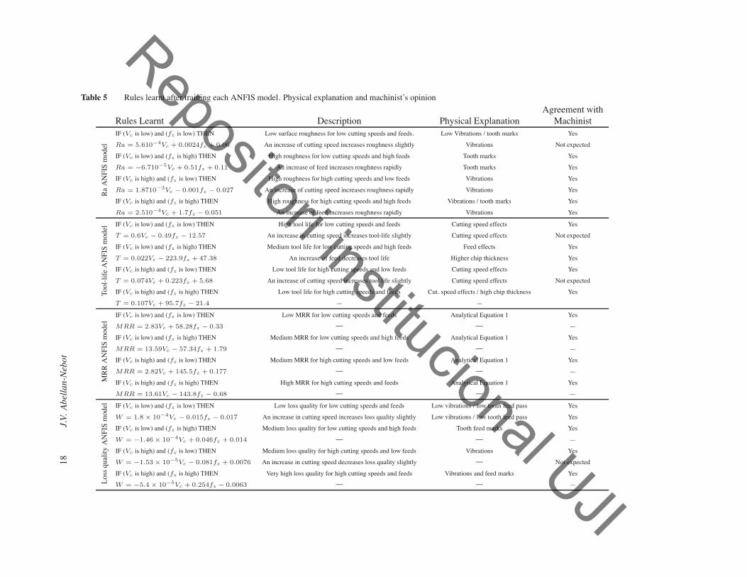
with the initial and final membership function for each variable, the rules learnt and thesurface response. Table 5 shows the rules learnt after training each ANFIS model, with itsphysical explanation and the machinist’s opinion.

Table 3 Characteristics of the Soft Computing methods applied.ANFIS modelsInputs 2 Outputs 1Rules 4 Training Hybrid optimisationInput MF type Gaussian MF per input 2Output MF type Linear MF per input 4AND method Prod OR method MaxDefuzzification Weighted averageGenetic AlgorithmNumber variables 2 Crossover fraction 0.8Population size 20 Elite count 2Stall generations Infinite Mutation function GaussianStall time Infinite Selection function StochasticGenerations 150 Initial ranges Vc = [100, 200]

fz = [0.04, 0.12]MF: Membership Functions

5.4 Optimisation Results

After modelling the machining process, the final desirability function can be defined asa function of Vc and fz . The optimal cutting parameter to maximise the overall desirabilitycan be obtained through an optimisation algorithm. A genetic algorithm with the maincharacteristics shown in Table 3 was applied for cutting parameter optimisation. After150 generations, the optimal cutting parameters were Vc = 165 m/min and fz = 0.11mm, with an overall desirability function of 0.512. In order to test experimentally theoverall desirability function at the optimal cutting parameters, an experimental run withthese cutting conditions was conducted, and a final desirability value of 0.536was obtained.Therefore, the theoretical results estimated a desirability increase of 10.1%, from 0.465 atVc = 200 m/min and fz = 0.08 mm (machinist’s approach) to 0.512 (soft computingapproach). However, the experimental results showed an increase of the overall desirabilityfunction from 0.505 (machinist’s approach) to 0.536 (soft computing approach), whichmeans an increase of 6.1%. The prediction error on the overall desirability function from10.1% to 6.1% could be explained due to modelling errors, especially in modelling surfaceroughness and loss quality, which could be more complex than the estimated ones.

6 Conclusions

In this paper, a comparison between traditional cutting parameter optimisation using ex-pert machinist knowledge and an experimental optimisation procedure based on Soft Com-puting methods has been reported. The presented experimental optimisation procedure hasbeen composed of two steps. First, the modelling of the process variables of interest such asmaterial removal rate, surface roughness, cutting tool life and loss quality of part accuracy



Table 4 ANFIS process models for surface roughness (Ra), Tool-life (T) ,material removal rate(MRR) and loss quality (W)

Initial Membership Final Membership3-D Model functions functions

RaANFISmodel

100 150 200

0

0.2

0.4

0.6

0.8

1

Vc (m/min)

Deg

ree

of m

embe

rshi

p

0.05 0.1

0

0.2

0.4

0.6

0.8

1

fz (mm)

Deg

ree

of m

embe

rshi

p

100 150 200

0

0.2

0.4

0.6

0.8

1

Vc (m/min)

Deg

ree

of m

embe

rshi

p

0.05 0.1

0

0.2

0.4

0.6

0.8

1

fz (mm)

Deg

ree

of m

embe

rshi

p

Rules LearntIF (Vc is low) and (fz is low) THENRa = 5.610−4Vc + 0.0024fz + 0.06

IF (Vc is low) and (fz is high) THENRa = −6.710−5Vc + 0.51fz + 0.11

IF (Vc is high) and (fz is low) THENRa = 1.8710−3Vc − 0.001fz − 0.027

IF (Vc is high) and (fz is high) THENRa = 2.510−4Vc + 1.7fz − 0.051

Tool-lifeANFISmodel

100 150 200

0

0.2

0.4

0.6

0.8

1

Vc (m/min)

Deg

ree

of m

embe

rshi

p

0.05 0.1

0

0.2

0.4

0.6

0.8

1

fz (mm)

Deg

ree

of m

embe

rshi

p

100 150 200

0

0.2

0.4

0.6

0.8

1

Vc (m/min)

Deg

ree

of m

embe

rshi

p

0.05 0.1

0

0.2

0.4

0.6

0.8

1

fz (mm)

Deg

ree

of m

embe

rshi

p

Rules LearntIF (Vc is low) and (fz is low) THEN T = 0.6Vc − 0.49fz − 12.57

IF (Vc is low) and (fz is high) THEN T = 0.022Vc − 223.9fz + 47.38

IF (Vc is high) and (fz is low) THEN T = 0.074Vc + 0.223fz + 5.68

IF (Vc is high) and (fz is high) THEN T = 0.107Vc + 95.7fz − 21.4

MRR

ANFISmodel

100 150 200

0

0.2

0.4

0.6

0.8

1

Vc (m/min)

Deg

ree

of m

embe

rshi

p

0.05 0.1

0

0.2

0.4

0.6

0.8

1

fz (mm)

Deg

ree

of m

embe

rshi

p

100 150 200

0

0.2

0.4

0.6

0.8

1

Vc (m/min)

Deg

ree

of m

embe

rshi

p

0.05 0.1

0

0.2

0.4

0.6

0.8

1

fz (mm)

Deg

ree

of m

embe

rshi

p

Rules LearntIF (Vc is low) and (fz is low) THENMRR = 2.83Vc + 58.28fz − 0.33

IF (Vc is low) and (fz is high) THENMRR = 13.59Vc − 57.34fz + 1.79

IF (Vc is high) and (fz is low) THENMRR = 2.82Vc + 145.5fz + 0.177

IF (Vc is high) and (fz is high) THENMRR = 13.61Vc − 143.8fz − 0.68

LossqualityANFISmodel

100 150 200

0

0.2

0.4

0.6

0.8

1

Vc (m/min)

Deg

ree

of m

embe

rshi

p

0.05 0.1

0

0.2

0.4

0.6

0.8

1

fz (mm)

Deg

ree

of m

embe

rshi

p

100 150 200

0

0.2

0.4

0.6

0.8

1

Vc (m/min)

Deg

ree

of m

embe

rshi

p

0.05 0.1

0

0.2

0.4

0.6

0.8

1

fz (mm)

Deg

ree

of m

embe

rshi

p

Rules LearntIF (Vc is low) and (fz is low) THENW = 1.810−4Vc − 0.015fz − 0.017

IF (Vc is low) and (fz is high) THENW = −1.4610−4Vc + 0.046fz + 0.014

IF (Vc is high) and (fz is low) THENW = −1.5310−5Vc − 0.081fz + 0.0076

IF (Vc is high) and (fz is high) THENW = −5.410−5Vc + 0.254fz − 0.0063


18J.V.Abellan-Nebot

Table 5 Rules learnt after training each ANFIS model. Physical explanation and machinist’s opinionAgreement with

Rules Learnt Description Physical Explanation Machinist

RaANFISmodel

IF (Vc is low) and (fz is low) THEN Low surface roughness for low cutting speeds and feeds. Low Vibrations / tooth marks Yes

Ra = 5.610−4Vc + 0.0024fz + 0.06 An increase of cutting speed increases roughness slightly Vibrations Not expected

IF (Vc is low) and (fz is high) THEN High roughness for low cutting speeds and high feeds Tooth marks Yes

Ra = −6.710−5Vc + 0.51fz + 0.11 An increase of feed increases roughness rapidly Tooth marks Yes

IF (Vc is high) and (fz is low) THEN High roughness for high cutting speeds and low feeds Vibrations Yes

Ra = 1.8710−3Vc − 0.001fz − 0.027 An increase of cutting speed increases roughness rapidly Vibrations Yes

IF (Vc is high) and (fz is high) THEN High roughness for high cutting speeds and high feeds Vibrations / tooth marks Yes

Ra = 2.510−4Vc + 1.7fz − 0.051 An increase of feed increases roughness rapidly Vibrations Yes

Tool-lifeANFISmodel IF (Vc is low) and (fz is low) THEN High tool life for low cutting speeds and feeds Cutting speed effects Yes

T = 0.6Vc − 0.49fz − 12.57 An increase in cutting speed increases tool-life slightly Cutting speed effects Not expected

IF (Vc is low) and (fz is high) THEN Medium tool life for low cutting speeds and high feeds Feed effects Yes

T = 0.022Vc − 223.9fz + 47.38 An increase of feed decreases tool life Higher chip thickness Yes

IF (Vc is high) and (fz is low) THEN Low tool life for high cutting speeds and low feeds Cutting speed effects Yes

T = 0.074Vc + 0.223fz + 5.68 An increase of cutting speed increases tool life slightly Cutting speed effects Not expected

IF (Vc is high) and (fz is high) THEN Low tool life for high cutting speeds and feeds Cut. speed effects / high chip thickness Yes

T = 0.107Vc + 95.7fz − 21.4 — —

MRR

ANFISmodel

IF (Vc is low) and (fz is low) THEN Low MRR for low cutting speeds and feeds Analytical Equation 1 Yes

MRR = 2.83Vc + 58.28fz − 0.33 — — —

IF (Vc is low) and (fz is high) THEN Medium MRR for low cutting speeds and high feeds Analytical Equation 1 Yes

MRR = 13.59Vc − 57.34fz + 1.79 — — —

IF (Vc is high) and (fz is low) THEN Medium MRR for high cutting speeds and low feeds Analytical Equation 1 Yes

MRR = 2.82Vc + 145.5fz + 0.177 — — —

IF (Vc is high) and (fz is high) THEN High MRR for high cutting speeds and feeds Analytical Equation 1 Yes

MRR = 13.61Vc − 143.8fz − 0.68 — — —

LossqualityANFISmodel IF (Vc is low) and (fz is low) THEN Low loss quality for low cutting speeds and feeds Low vibrations / low tooth feed pass Yes

W = 1.8 × 10−4Vc − 0.015fz − 0.017 An increase in cutting speed increases loss quality slightly Low vibrations / low tooth feed pass Yes

IF (Vc is low) and (fz is high) THEN Medium loss quality for low cutting speeds and high feeds Tooth feed marks Yes

W = −1.46 × 10−4Vc + 0.046fz + 0.014 — — —

IF (Vc is high) and (fz is low) THEN Medium loss quality for high cutting speeds and low feeds Vibrations Yes

W = −1.53 × 10−5Vc − 0.081fz + 0.0076 An increase in cutting speed decreases loss quality slightly — Not expected

IF (Vc is high) and (fz is high) THEN Very high loss quality for high cutting speeds and feeds Vibrations and feed marks Yes

W = −5.4 × 10−5Vc + 0.254fz − 0.0063 — — —



have been conducted by Adaptive Neuro-fuzzy Inference Systems. This soft computing ap-proach models each process variable by rules extracted from the experimental data whichcan be interpreted and verified by the expert machinist in order to have a better understand-ing of the process. As a second step, it was defined a multi-objective function using thedesirability function approach and a Genetic Algorithm was applied to optimise the overalldesirability function and find the optimal cutting parameters which best define the trade-offamong production rate, cutting costs and part accuracy. The theoretical results predictedan increase on the multi-objective function of 10.1% by the application of the experimentalcutting parameter approach presented in the paper instead of the parameter selection by theexpert machinist. After a validation run, the increase on the multi-objective function wasproved to be 6.1%. The error between theoretical and experimental results were assumedto be due to modelling errors, especially in the surface roughness and loss quality models.

(a) (b)

Figure 7 (a) Mean population value and best sample at each generation during the optimisa-tion by GA. (b) Comparison between the overall desirability function obtained by using the expertmachinist knowledge and the Soft Computing method proposed.

References

Chiang, S. T., Liu, D. I., Lee, A. C. and Chieng, W. H. (1995) ‘Adaptive-control optimiza-tion in end milling using neural networks’, International Journal of Machine Tools andManufacture, Vol. 35, No. 4, pp. 637–660.

Chien, W. T. and Chou, C. Y. (2001) ‘The predictive model for machinability of 304 stain-less steel’, Journal of Materials Processing Technology, Vol. 118, No. 1-3, pp. 442–447.

Cus, F. and Balic, J. (2003) ‘Optimization of cutting process by ga approach’, Robotics andComputer-Integrated Manufacturing, Vol. 19, No. 1-2, pp. 113–121.

Derringer, G. and Suich, R. (1980) ‘Simultaneous-optimization of several response vari-ables’, Journal of Quality Technology, Vol. 12, No. 4, pp. 214–219.

Ghani, J. A., Choudhury, I. A. and Hassan, H. H. (2004) ‘Application of taguchi method inthe optimization of end milling parameters’, Journal of Materials Processing Technology,Vol. 145, No. 1, pp. 84–92.

Holland, J. (1975) Adaptation in natural and artificial systems, Ann Arbor, USA: TheUniversity of Michigan Press.



Ip, R. W. L., Lau, H. C. W. and Chan, F. T. S. (2003) ‘An economical sculptured surfacemachining approach using fuzzy models and ball-nosed cutters’, Journal of MaterialsProcessing Technology, Vol. 138, pp. 579–585.

ISO (1989) ‘Tool life test in milling, part 1: Face milling’, International Standard Organi-zation (ISO).

Jain, L. C. andMartin, N. M. (1998)Fusion of Neural Networks, Fuzzy Systems and GeneticAlgorithms: Industrial Applications, Florida, CRC Press LLC edn.

Jang, J. S. R. (1993) ‘Anfis - adaptive-network-based fuzzy inference system’, Ieee Trans-actions on Systems Man and Cybernetics, Vol. 23, No. 3, pp. 665–685.

Juan, H., Yu, S. F. and Lee, B. Y. (2003) ‘The optimal cutting-parameter selection of pro-duction cost in hsm for skd61 tool steels’, International Journal of Machine Tools andManufacture, Vol. 43, No. 7, pp. 679–686.

Liu, Y. M. andWang, C. J. (1999a) ‘Neural network based adaptive control and optimisationin the milling process’, International Journal of Advanced Manufacturing Technology,Vol. 15, No. 11, pp. 791–795.

Liu, Y. M., Zuo, L. and Wang, C. J. (1999b) ‘Intelligent adaptive control in milling pro-cesses’, International Journal of Computer Integrated Manufacturing, Vol. 12, No. 5, pp.453–460.

Mukherjee, I. and Ray, P. K. (2006) ‘A review of optimization techniques in metal cuttingprocesses’, Computers and Industrial Engineering, Vol. 50, No. 1-2, pp. 15–34.

NIST/SEMATECH (2006) ‘Nist/sematech e-handbook of statistical methods’, ElectronicCitation.

Siller, H. R., Vila, C., Rodriguez, C. A. and Abellan, J. V. (2008) ‘Study of face millingof hardened aisi d3 steel with a special design of carbide tool’, International Journal ofAdvanced Manufacturing Technology.

Suresh, P. V. S., Rao, P. V. and Deshmukh, S. G. (2002) ‘A genetic algorithmic approach foroptimization of surface roughness prediction model’, International Journal of MachineTools and Manufacture, Vol. 42, No. 6, pp. 675–680.

Trent, E.M. andWright, P. K. (2000)Metal Cutting, Butterworth Heinemann, fourth editionedn.

Wang, J. and Kusiak, A. (2000) Computational Intelligence in Manufacturing Handbook.Zhang, J. Z., Chen, J. C. and Kirby, E. D. (2007) ‘Surface roughness optimization in anend-milling operation using the taguchi design method’, Journal of Materials ProcessingTechnology, Vol. 184, No. 1-3, pp. 233–239.

Zuperl, U. and Cus, F. (2003) ‘Optimization of cutting conditions during cutting by usingneural networks’, Robotics and Computer-Integrated Manufacturing, Vol. 19, No. 1-2,pp. 189–199.


cutting parameters optimisation in milling: expert

Documents