cup coproducts in hopf cyclic cohomology
TRANSCRIPT
J. Homotopy Relat. Struct.DOI 10.1007/s40062-013-0064-1
Cup coproducts in Hopf cyclic cohomology
Mohammad Hassanzadeh · Masoud Khalkhali
Received: 19 March 2012 / Accepted: 19 April 2013© Tbilisi Centre for Mathematical Sciences 2013
Abstract We define cup coproducts for Hopf cyclic cohomology of Hopf algebrasand for its dual theory. We show that for universal enveloping algebras and groupalgebras our coproduct recovers the standard coproducts on Lie algebra homologyand group homology, respectively.
Keywords Cyclic cohomology · Hopf algebras · Noncommutative geometry
Mathematics Subject Classification (2010) 19D55 · 16T05 · 11M55
1 Introduction
In this paper we define cup coproducts for Hopf cyclic cohomology of Hopf algebras byestablishing Künneth formulas for Hopf cyclic cohomology. Cup product for cycliccohomology of algebras was first defined by Connes in [4]. Künneth formulas and(co)products for cyclic theory of algebras has been established by several authors [1,2,8,16,17,19] (cf. also Loday’s book [24] and references therein for a full account). Eversince the discovery of Hopf cyclic cohomology by Connes and Moscovici and withcomputations carried on in [6,7], it was clear that this theory and its dual counterpart[20] is a noncommutative analogue of Lie algebra homology and group homology. Thisof course poses a natural question: to what extent cup products in Lie algebra and group
Communicated by Jonathan Rosenberg.
M. Hassanzadeh (B) ·M. KhalkhaliDepartment of Mathematics, University of Western Ontario, London, ON, Canadae-mail: [email protected]
M. Khalkhalie-mail: [email protected]
123
M. Hassanzadeh, M. Khalkhali
cohomology can be extended to Hopf cyclic cohomology. This question is answered inthis paper. We use the theory of cyclic modules and the definition of Hopf cyclic coho-mology (with coefficients) in terms of cyclic modules [6,13] to define our coproductsin a natural way via Eilenberg–Zilber isomorphisms for cyclic modules. This gives usan external coproduct. By specifying to cocommutative Hopf algebras we then definecup coproducts for Hopf cyclic (co)homology of cocommutative Hopf algebras.
This paper is organized as follows. In Sects. 2 and 3 we recall the Eilenberg–Zilber isomorphism and Künneth formula for cyclic homology. In Sect. 4 we recallthe definition of Hopf cyclic cohomology with coefficients in an stable anti-Yetter–Drinfeld module and work out the Eilenberg–Zilber isomorphism and Künneth formulain the context of Hopf cyclic cohomology. In Sect. 5 we define external coproductsfor Hopf cyclic cohomology and in Sect. 6 by restricting to cocommutative Hopfalgebras we obtain internal coproducts on Hopf cyclic cohomology. It is known thatwhen restricted to universal enveloping algebras, Hopf cyclic cohomology reducesto Lie algebra homology [6]. In Sect. 6 we show that under these isomorphisms ourcoproduct coincides with the coproduct in Lie algebra homology. In Sect. 7 we lookat the dual Hopf cyclic homology as defined in [20] and define a coproduct on it.It is shown in [20] that when restricted to group algebras, Hopf cyclic homology isisomorphic to group homology. In this section we check that under this isomorphismour coproduct coincides with coproduct in group homology.
It should be mentioned that the term cup product is also used for a different type ofoperation in Hopf cyclic theory. Thus the cup products defined and studied in [11,13–15,22,25] involve an action of a Hopf algebra on a (co)algebra and is a pairing betweenHopf cyclic cohomology of the given (co)algebra and Hopf cyclic cohomology of theacting Hopf algebra. This operation is in fact an extension of Connes–Moscovicvi’scharacteristic map from [7].
2 Eilenberg–Zilber isomorphisms
In this section we recall the Eilenberg–Zilber isomorphisms for Hochschild, cyclicand periodic cyclic (co)homology of (co)cyclic modules where they will be usedcrucially in future sections [1,10,21]. Given a (co)cyclic module (C, δ, s, τ ) [3,24],where δ, s and τ are (co)faces, (co)degeneracies and (co)cyclic maps respectively, wedenote its Hochschild differential in cohomology by bn =∑n
i=0(−1)iδi , and Connes’differential by Bn = (
∑ni=0(−1)niτ i
n)snτn(1 − τn). Any (co)cyclic module definesa mixed complex (C, b, B) in a natural way [3,18,24]. Suppose (Cn, δn
i , sni , τ
n) and(C ′n, δ′ni , s′ni , τ ′n) are two cocyclic modules. The diagonal C × C ′ is the cocyclicmodule ((C × C ′)n, δn
i ⊗ δ′ni , sni ⊗ s′ni , τn ⊗ τ ′n) where
(C × C ′)n = Cn ⊗ C ′n .The tensor product complex C ⊗ C ′ given by
(C ⊗ C ′)n =⊕
p+q=n
C p ⊗ C ′q ,
is not a cocyclic module but it has a mixed complex structure given by
123
Cup coproducts in Hopf cyclic cohomology
bn =⊕
i+ j=n
(bi ⊗ id j + (−1) j idi ⊗ b′j ),
and similarly for B.We have two natural maps between these complexes. The Alexander–Whitney map
AWn : (C ⊗ C ′)n −→ (C × C ′)n,
is given by
AWn =⊕
i+ j=n
AWi, j , (2.1)
where
AWi, j : Ci ⊗ C ′ j −→ Cn ⊗ C ′n,
are defined by
AWi, j = δnnδ
n−1n−1 · · · δi+1
i+1 ⊗ δn0δ
n−10 · · · δi+1
0 . (2.2)
The Shuffle map
shn : (C × C ′)n −→ (C ⊗ C ′)n,
is given by
shn =⊕
i+ j=n
shi, j , (2.3)
where
shi, j : (C × C ′)n −→ Ci ⊗ C ′ j ,
are defined by
shi, j =∑
σ
sign(σ )siσ(i+1) · · · sn−1
σ(n) ⊗ s jσ(1) · · · sn−1
σ(i) , (2.4)
and σ runs over all (i, j)-shuffles. By an (i, j) shuffle we mean a permutation σ onelements {1, 2, . . . , n} such that
σ(1) < σ(2) < · · · < σ(i), σ (i + 1) < σ(i + 2) < · · · < σ(n).
One has [b, sh] = 0 and [b, AW ] = 0 in the normalized setting [3,24]. It can beshown that
123
M. Hassanzadeh, M. Khalkhali
sh ◦ AW = id, AW ◦ sh = bh + hb + id,
for some chain homotopy map h [24]. So they induce inverse isomorphisms onHochschild cohomology, called the Eilenberg–Zilber isomorphism:
H Hn(C ⊗ C ′) ∼= H Hn(C × C ′) ∀n ≥ 0. (2.5)
In the dual case of cyclic modules, the map
AWn : (C × C ′)n −→ (C ⊗ C ′)n,
is given by
AWn =⊕
i+ j=n
AWi, j , (2.6)
where AWi, j : Cn ⊗ C ′n −→ Ci ⊗ C ′j are given by
AWi, j = δi+1i+1δ
i+2i+2 · · · δn
n ⊗ δi+10 δi+2
0 · · · δn0 . (2.7)
Also
shn : (C ⊗ C ′)n −→ (C × C ′)n,
is given by
shn =⊕
i+ j=n
shi, j , (2.8)
where shi, j : Ci ⊗ C ′j −→ Cn ⊗ C ′n can be defined as:
shi, j =∑
σ
sign(σ )sn−1σ(n) · · · si
σ(i+1) ⊗ sn−1σ(i) · · · s j
σ(1). (2.9)
Now we state the Eilenberg–Zilber isomorphism for cyclic cohomology. To thisend, we define another map namely the cyclic shuffle map as follows [23,24]. First wedefine an (i, j)-cyclic shuffle. Let i, j, n ∈ N with n = i+ j . Consider the permutationσ on the n elements {1, . . . , n} obtained by first performing a cyclic permutation ptimes on {1, . . . , i} and a cyclic permutation q times on {i + 1, . . . , i + j} and thereafter applying an (i, j)-shuffle to the combined result. We call σ an (i, j)-cyclic shuffleif 1 appears before i+1 in the resulting sequence. One can define another map namelysh′ which is in fact a cyclic version of the shuffle map:
sh′n : (C × C ′)n −→ (C ⊗ C ′)n−2,
123
Cup coproducts in Hopf cyclic cohomology
where
sh′n =⊕
i+ j=n
sh′i, j , (2.10)
and sh′i, j : Cn ⊗ C ′n −→ Ci−1 ⊗ C ′ j−1, are given by
sh′i, j =∑
σ
sign(σ )si−1i−p−1τ
p+1i si
σ(i+1) · · · sn−1σ(n)⊗s j−1
j−q−1τq+1j s j
σ(1) · · · sn−1σ(i) . (2.11)
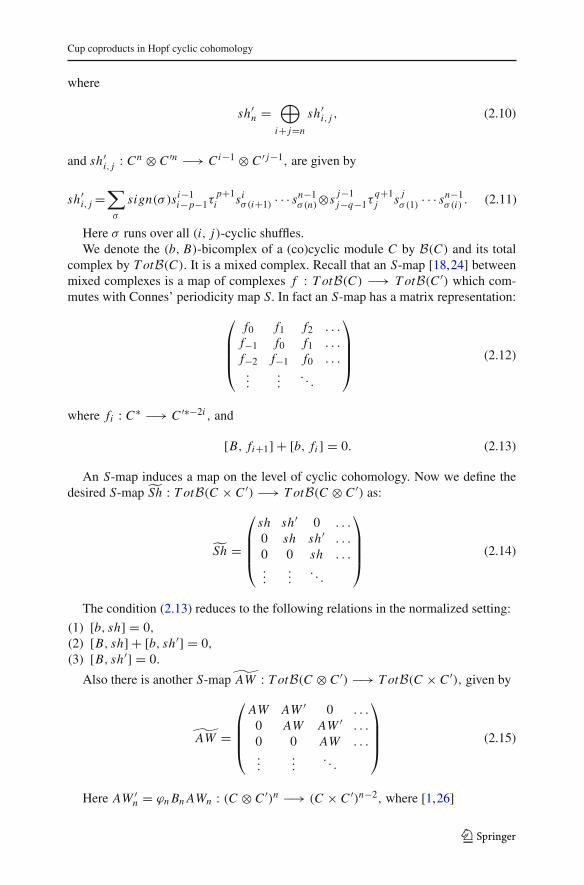
Here σ runs over all (i, j)-cyclic shuffles.We denote the (b, B)-bicomplex of a (co)cyclic module C by B(C) and its total
complex by T otB(C). It is a mixed complex. Recall that an S-map [18,24] betweenmixed complexes is a map of complexes f : T otB(C) −→ T otB(C ′) which com-mutes with Connes’ periodicity map S. In fact an S-map has a matrix representation:
⎛
⎜⎜⎜⎝
f0 f1 f2 . . .
f−1 f0 f1 . . .
f−2 f−1 f0 . . ....
.... . .
⎞
⎟⎟⎟⎠
(2.12)
where fi : C∗ −→ C ′∗−2i , and
[B, fi+1] + [b, fi ] = 0. (2.13)
An S-map induces a map on the level of cyclic cohomology. Now we define thedesired S-map Sh : T otB(C × C ′) −→ T otB(C ⊗ C ′) as:
Sh =
⎛
⎜⎜⎜⎝
sh sh′ 0 . . .
0 sh sh′ . . .0 0 sh . . ....
.... . .
⎞
⎟⎟⎟⎠
(2.14)
The condition (2.13) reduces to the following relations in the normalized setting:
(1) [b, sh] = 0,(2) [B, sh] + [b, sh′] = 0,(3) [B, sh′] = 0.
Also there is another S-map AW : T otB(C ⊗ C ′) −→ T otB(C × C ′), given by
AW =
⎛
⎜⎜⎜⎝
AW AW ′ 0 . . .
0 AW AW ′ . . .0 0 AW . . ....
.... . .
⎞
⎟⎟⎟⎠
(2.15)
Here AW ′n = ϕn Bn AWn : (C ⊗ C ′)n −→ (C × C ′)n−2, where [1,26]
123
M. Hassanzadeh, M. Khalkhali
ϕn =∑
(−1)n−p−q+σ(α,β)(sβq+n−p−q · · · sβ1+n−p−qsn−p−q−1δn−q+1 · · · δn)
⊗(sαp+1+n−p−q · · · sα1+n−p−qδn−p−q · · · δn−q−1).
The sum is taken over all 0 ≤ q ≤ n− 1, 0 ≤ p ≤ n− q − 1, and (α, β) runs overall (p + 1, q)-shuffles where σ(α, β) =∑
(αi − i + 1). One can show [1]
Sh ◦ AW = id, AW ◦ Sh = (b + B) ◦ h + h ◦ (b + B)+ id,
for some homotopy map h : C⊗C ′ −→ C×C ′. Thus we obtain the Eilenberg–Zilberisomorphism in cyclic cohomology [1,21,24]:
HC∗(C × C ′) ∼= HC∗(C ⊗ C ′). (2.16)
In the case of cyclic modules, one can define
sh′n : (C ⊗ C ′)n −→ (C × C ′)n+2 ∀n ≥ 0, (2.17)
and
AW ′n : (C × C ′)n −→ (C ⊗ C ′)n+2 ∀n ≥ 0. (2.18)
This enables us to have the S-maps Sh : T otB(C ⊗ C ′) −→ T otB(C × C ′),and AW : T otB(C × C ′) −→ T otB(C ⊗ C ′) which induce the Eilenberg–Zilberisomorphism in cyclic homology.
We have the Eilenberg–Zilber isomorphism for periodic cyclic cohomology asfollows. One knows that lim−→T ot2n+∗B(C) = ⊕n≥0C2n+∗, where ∗ = 0, 1 and thedirect limit is with respect to Connes’ periodicity map S. Since direct limit commuteswith homology we have
lim−→HC2n+∗(C) = lim−→H(T ot2n+∗B(C)) = H(lim−→T ot2n+∗B(C))= H(⊕n≥0C2n+∗) = H P∗(C),
where ∗ = 0, 1. Since
H P∗(C ⊗ C ′) = lim−→HC2n+∗(C ⊗ C ′) ∼= lim−→HC2n+∗(C × C ′) = H P∗(C × C ′),
we obtain the Eilenberg–Zilber isomorphism for periodic cyclic cohomology:
H P∗(C ⊗ C ′) ∼= H P∗(C × C ′), (2.19)
The explicit maps which induce the isomorphism (2.19), are infinite matrix versionsof Sh and AW .
There is an obstacle to get the Eilenberg–Zilber isomorphism for periodic cyclichomology. The problem comes from the fact that homology does not commute with
123
Cup coproducts in Hopf cyclic cohomology
inverse limit in general. The Mittag-Leffler condition [9] on the inverse system(HC(C)[−2m], S)m guarantees the commutativity of homology and inverse limit.If we have this condition, with a similar argument we obtain
H Pn(C ⊗ C ′) ∼= H Pn(C × C ′).
3 Künneth formulas
In this section we recall the Künneth formula for Hochschild and cyclic (co)homologyof (co)cyclic modules and introduce a formula for the periodic case. If C and C ′are cocyclic objects in the category of vector spaces, we have the following Künnethformula:
H Hn(C ⊗ C ′)∼=⊕
p+q=n
H H p(C)⊗ H Hq(C ′) ∀ n ≥ 0. (3.1)
The above isomorphism is induced by the shuffle map and following natural map[24]
I : [α] ⊗ [β] −→ [α ⊗ β]. (3.2)
The same maps induce an isomorphism for Hochschild homology of cyclic modules.In the case of cyclic homology we do not have an isomorphism similar to (3.1).
Instead, there is a short exact sequence [2,16,19,24]:
0 −→ T otnB(C ⊗ C ′) I−−−−→⊕
i+ j=n
T otiB(C)⊗ T ot jB(C ′) S⊗id−id⊗S−−−−−−−→⊕
i+ j=n−2
T otiB(C)⊗ T ot jB(C ′) −→ 0. (3.3)
The map I is called the Künneth map which can be defined as follows. LetT otB(C) = k[u] ⊗ C , where |u| = 2, T otB(C ′) = k[u′] ⊗ C ′ where |u′| = 2,and T otB(C ⊗ C ′) = k[v] ⊗ C ⊗ C ′ where |v| = 2. One can define the map I as[2,24]:
I(vn) =∑
p+q=n
u pu′q . (3.4)
From the Künneth short exact sequence (3.3), we get the following long exactsequence in homology:
... −→ HCn(C ⊗ C ′) I−−−−→⊕
i+ j=n
HCi (C)⊗ HC j (C′) S⊗id−id⊗S−−−−−−−→
⊕
i+ j=n−2
HCi (C)⊗ HC j (C′) ∂−−−−→ HCn−1(C ⊗ C ′) −→ ....
123
M. Hassanzadeh, M. Khalkhali
Similarly for cyclic cohomology, we have the following short exact sequence:
0 −→ T otn B(C ⊗ C ′) I−−−−→⊕
i+ j=n
T oti B(C)⊗ T ot j B(C ′) S⊗id−id⊗S−−−−−−−→⊕
i+ j=n+2
T oti B(C)⊗ T ot j B(C ′) −→ 0.
Consequently, we get the following long exact sequence in cohomology [2,18]:
... −→ HCn(C ⊗ C ′) I−−−−→⊕
p+q=n
HC p(C)⊗ HCq(C ′) S⊗id−id⊗S−−−−−−−→⊕
r+s=n+2
HCr (C)⊗ HCs(C ′) ∂−−−−→ HCn+2(C ⊗ C ′) −→ .... (3.5)
where ∂ is the connecting morphism of short exact sequences.Now we state the Künneth formula for the periodic case. One can find the formula
for algebras in [8]. Here we provide a similar argument in the general case of (co)cyclicmodules. Recall that a supercomplex is a Z2-graded vector space V = V0⊕V1 endowedwith linear maps ∂0 : V0 −→ V1 and ∂1 : V1 −→ V0 such that ∂0∂1 = 0 and ∂1∂0 = 0.
We denote the corresponding chain complex by V0∂0�∂1
V1, where its homology is a
Z2-graded vector space given by:
H0 = K er∂0/I m∂1, H1 = K er∂1/I m∂0.
For example the inverse limit lim←−T otB(C) is a supercomplex. In this case V =T ot Bn(C) , ∂ = B + b and we have lim←−T otB(C) = (∏ C2n)n≥0 ⊕ (∏ C2n+1)n≥0.
For cohomology, lim−→T otB(C) = V0 ⊕ V1 = (⊕C2n)n≥0 ⊕ (⊕C2n+1)n≥0. A mapof supercomplexes is a linear map f : V = V0 ⊕ V1 −→ W = W0 ⊕ W1 suchthat sends V0 to W0 and V1 to W1. If we have two supercomplexes V and W , thenV ⊗W is a supercomplex where (V ⊗W )0 = (V0⊗W0)⊕ (V1⊗W1) and (V ⊗W )1 =(V0 ⊗W1)⊕ (V1 ⊗W0). We define
∂V ⊗W0 =
(1⊗ ∂W
0 ∂V1 ⊗ 1
∂V0 ⊗ 1 −1⊗ ∂W
1
)
and ∂V ⊗W1 =
(1⊗ ∂W
1 ∂V1 ⊗ 1
∂V0 ⊗ 1 −1⊗ ∂W
0
)
(3.6)
The Künneth formula for supercomplexes holds:
H(X⊗Y ) ∼= H(X)⊗H(Y ).
We define the supercomplex map:
∇ : (lim←−T otB(C))⊗(lim←−T otB(C ′)) −→ lim←−T otB(C ⊗ C ′). (3.7)
123
Cup coproducts in Hopf cyclic cohomology
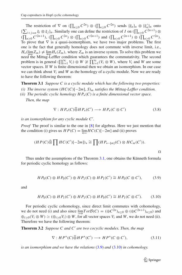
The restriction of ∇ on (∏
n≥0 C2n) ⊗ (∏n≥0 C ′2n) sends {ξn}n ⊗ {ξ ′n}n onto{∑i+ j=n ξi ⊗ ξ j }n . Similarly one can define the restriction of I on (
∏n≥0 C2n+1)⊗
(∏
n≥0 C ′2n+1), (∏
n≥0 C2n) ⊗ (∏n≥0 C ′2n+1) and (∏
n≥0 C2n+1) ⊗ (∏n≥0 C ′2n).To prove that ∇ is a quasi-isomorphism, we have two major problems. The firstone is the fact that generally homology does not commute with inverse limit, i.e.,H∗(lim←−Zm) �= lim←−H∗(Zm), where Zm is an inverse system. To solve this problem weneed the Mittag-Leffler condition which guarantees the commutativity. The secondproblem is in general (
∏∞i=1 Vi )⊗ W �
∏∞i=1(Vi ⊗ W ), where Vi and W are some
vector spaces. If W is finite dimensional then we obtain an isomorphism. In our casewe can think about Vi and W as the homology of a cyclic module. Now we are readyto have the following theorem:
Theorem 3.1 Suppose C is a cyclic module which has the following two properties:
(i) The inverse system (HC(C)[−2m], S)m satisfies the Mittag-Leffler condition.(ii) The periodic cyclic homology H P∗(C) is a finite dimensional vector space.
Then, the map
∇ : H P∗(C)⊗H P∗(C ′) −→ H P∗(C ⊗ C ′) (3.8)
is an isomorphism for any cyclic module C ′.Proof The proof is similar to the one in [8] for algebras. Here we just mention thatthe condition (i) gives us H P(C) = lim←−HC(C)[−2m] and (ii) proves
(H P(C)⊗∏
HC(C ′)[−2m])∗ ∼=∏(H P∗−[m](C)⊗ HCm(C
′)).
��Thus under the assumptions of the Theorem 3.1, one obtains the Künneth formula
for periodic cyclic homology as follows:
H P0(C)⊗ H P0(C′)⊕ H P1(C)⊗ H P1(C
′) ∼= H P0(C ⊗ C ′), (3.9)
and
H P0(C)⊗ H P1(C′)⊕ H P1(C)⊗ H P0(C
′) ∼= H P1(C ⊗ C ′). (3.10)
For periodic cyclic cohomology, since direct limit commutes with cohomology,we do not need (i) and also since lim−→T otB(C) = (⊕C2n)n≥0 ⊕ (⊕C2n+1)n≥0) and⊕i≥0(Vi ⊗W ) � (⊕i≥0Vi )⊗W , for all vector spaces Vi and W , we do not need (ii).Therefore we have the following theorem:
Theorem 3.2 Suppose C and C ′ are two cocyclic modules. Then, the map
∇ : H P∗(C)⊗H P∗(C ′) −→ H P∗(C ⊗ C ′), (3.11)
is an isomorphism and we have the relations (3.9) and (3.10) in cohomology.
123
M. Hassanzadeh, M. Khalkhali
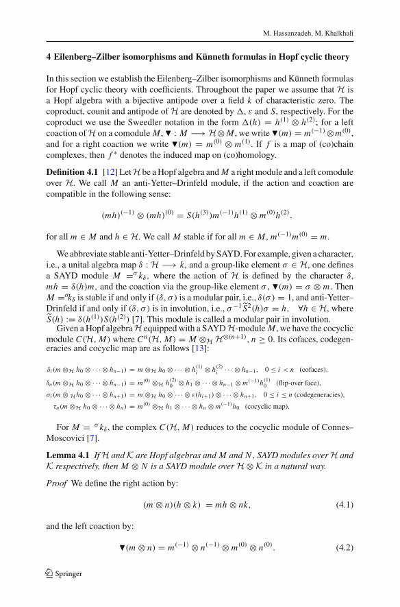
4 Eilenberg–Zilber isomorphisms and Künneth formulas in Hopf cyclic theory
In this section we establish the Eilenberg–Zilber isomorphisms and Künneth formulasfor Hopf cyclic theory with coefficients. Throughout the paper we assume that H isa Hopf algebra with a bijective antipode over a field k of characteristic zero. Thecoproduct, counit and antipode of H are denoted by , ε and S, respectively. For thecoproduct we use the Sweedler notation in the form (h) = h(1) ⊗ h(2); for a leftcoaction of H on a comodule M , � : M −→ H⊗M , we write �(m) = m(−1)⊗m(0),and for a right coaction we write �(m) = m(0) ⊗ m(1). If f is a map of (co)chaincomplexes, then f ∗ denotes the induced map on (co)homology.
Definition 4.1 [12] Let H be a Hopf algebra and M a right module and a left comoduleover H. We call M an anti-Yetter–Drinfeld module, if the action and coaction arecompatible in the following sense:
(mh)(−1) ⊗ (mh)(0) = S(h(3))m(−1)h(1) ⊗ m(0)h(2),
for all m ∈ M and h ∈ H. We call M stable if for all m ∈ M , m(−1)m(0) = m.
We abbreviate stable anti-Yetter–Drinfeld by SAYD. For example, given a character,i.e., a unital algebra map δ : H −→ k, and a group-like element σ ∈ H, one definesa SAYD module M =σ kδ, where the action of H is defined by the character δ,mh = δ(h)m, and the coaction via the group-like element σ , �(m) = σ ⊗ m. ThenM =σkδ is stable if and only if (δ, σ ) is a modular pair, i.e., δ(σ ) = 1, and anti-Yetter–Drinfeld if and only if (δ, σ ) is in involution, i.e., σ−1 S2(h)σ = h, ∀h ∈ H, whereS(h) := δ(h(1))S(h(2)) [7]. This module is called a modular pair in involution.
Given a Hopf algebra H equipped with a SAYD H-module M , we have the cocyclicmodule C(H,M) where Cn(H,M) = M ⊗H H⊗(n+1), n ≥ 0. Its cofaces, codegen-eracies and cocyclic map are as follows [13]:
δi (m ⊗H h0 ⊗ · · · ⊗ hn−1) = m ⊗H h0 ⊗ · · · ⊗ h(1)i ⊗ h(2)i · · · ⊗ hn−1, 0 ≤ i < n (cofaces),
δn(m ⊗H h0 ⊗ · · · ⊗ hn−1) = m(0) ⊗H h(2)0 ⊗ h1 ⊗ · · · ⊗ hn−1 ⊗ m(−1)h(1)0 (flip-over face),
σi (m ⊗Hh0 ⊗ · · · ⊗ hn+1) = m ⊗H h0 ⊗ · · · ⊗ ε(hi+1)⊗ · · · ⊗ hn+1, 0 ≤ i ≤ n (codegeneracies),
τn(m ⊗H h0 ⊗ · · · ⊗ hn) = m(0) ⊗H h1 ⊗ · · · ⊗ hn ⊗ m(−1)h0 (cocyclic map).
For M = σ kδ , the complex C(H,M) reduces to the cocyclic module of Connes–Moscovici [7].
Lemma 4.1 If H and K are Hopf algebras and M and N , SAYD modules over H andK respectively, then M ⊗ N is a SAYD module over H⊗K in a natural way.
Proof We define the right action by:
(m ⊗ n)(h ⊗ k) = mh ⊗ nk, (4.1)
and the left coaction by:
�(m ⊗ n) = m(−1) ⊗ n(−1) ⊗ m(0) ⊗ n(0). (4.2)
123
Cup coproducts in Hopf cyclic cohomology
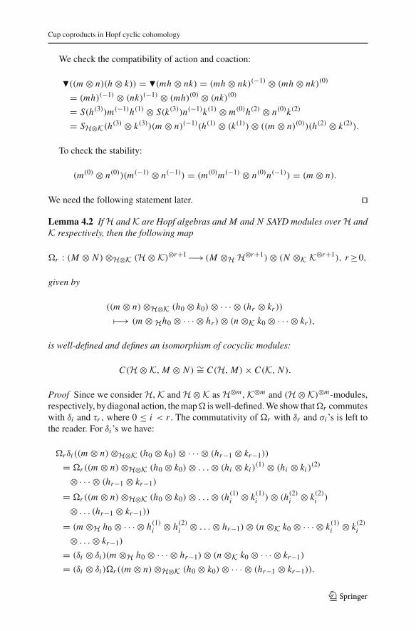
We check the compatibility of action and coaction:
�((m ⊗ n)(h ⊗ k)) = �(mh ⊗ nk) = (mh ⊗ nk)(−1) ⊗ (mh ⊗ nk)(0)
= (mh)(−1) ⊗ (nk)(−1) ⊗ (mh)(0) ⊗ (nk)(0)
= S(h(3))m(−1)h(1) ⊗ S(k(3))n(−1)k(1) ⊗ m(0)h(2) ⊗ n(0)k(2)
= SH⊗K(h(3) ⊗ k(3))(m ⊗ n)(−1)(h(1) ⊗ (k(1))⊗ ((m ⊗ n)(0))(h(2) ⊗ k(2)).
To check the stability:
(m(0) ⊗ n(0))(m(−1) ⊗ n(−1)) = (m(0)m(−1) ⊗ n(0)n(−1)) = (m ⊗ n).
We need the following statement later. ��Lemma 4.2 If H and K are Hopf algebras and M and N SAYD modules over H andK respectively, then the following map
�r : (M ⊗ N )⊗H⊗K (H⊗K)⊗r+1−→(M ⊗H H⊗r+1)⊗ (N ⊗K K⊗r+1), r≥0,
given by
((m ⊗ n)⊗H⊗K (h0 ⊗ k0)⊗ · · · ⊗ (hr ⊗ kr ))
−→ (m ⊗ Hh0 ⊗ · · · ⊗ hr )⊗ (n ⊗K k0 ⊗ · · · ⊗ kr ),
is well-defined and defines an isomorphism of cocyclic modules:
C(H⊗K,M ⊗ N ) ∼= C(H,M)× C(K, N ).
Proof Since we consider H, K and H⊗K as H⊗m , K⊗m and (H⊗K)⊗m-modules,respectively, by diagonal action, the map� is well-defined. We show that�r commuteswith δi and τr , where 0 ≤ i < r . The commutativity of �r with δr and σi ’s is left tothe reader. For δi ’s we have:
�rδi ((m ⊗ n)⊗H⊗K (h0 ⊗ k0)⊗ · · · ⊗ (hr−1 ⊗ kr−1))
= �r ((m ⊗ n)⊗H⊗K (h0 ⊗ k0)⊗ . . .⊗ (hi ⊗ ki )(1) ⊗ (hi ⊗ ki )
(2)
⊗ · · · ⊗ (hr−1 ⊗ kr−1)
= �r ((m ⊗ n)⊗H⊗K (h0 ⊗ k0)⊗ . . .⊗ (h(1)i ⊗ k(1)i )⊗ (h(2)i ⊗ k(2)i )
⊗ . . . (hr−1 ⊗ kr−1))
= (m ⊗H h0 ⊗ · · · ⊗ h(1)i ⊗ h(2)i ⊗ . . .⊗ hr−1)⊗ (n ⊗K k0 ⊗ · · · ⊗ k(1)i ⊗ k(2)i
⊗ . . .⊗ kr−1)
= (δi ⊗ δi )(m ⊗H h0 ⊗ · · · ⊗ hr−1)⊗ (n ⊗K k0 ⊗ · · · ⊗ kr−1)
= (δi ⊗ δi )�r ((m ⊗ n)⊗H⊗K (h0 ⊗ k0)⊗ · · · ⊗ (hr−1 ⊗ kr−1)).
123
M. Hassanzadeh, M. Khalkhali
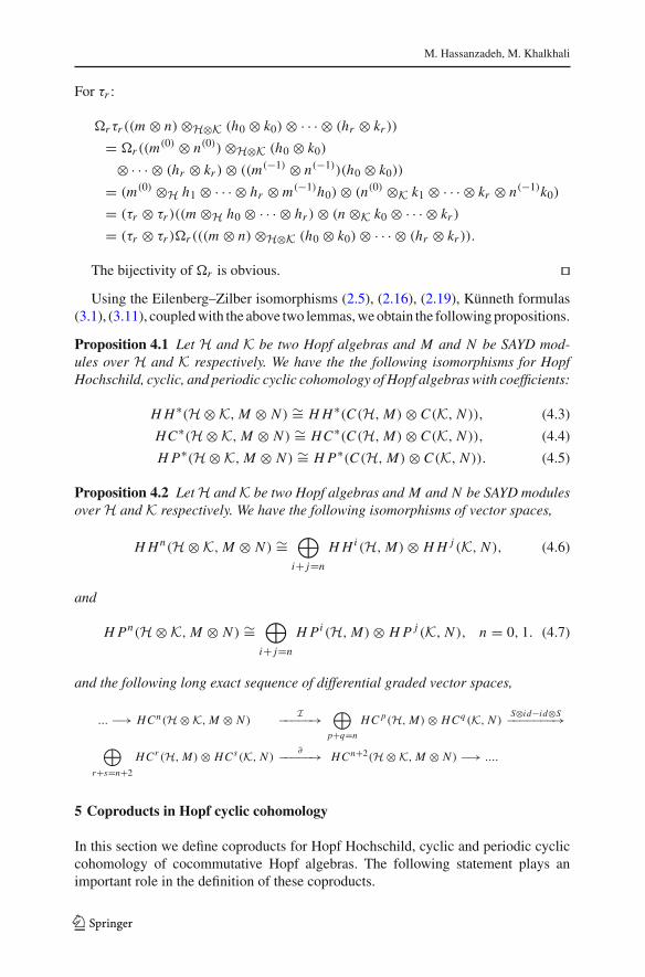
For τr :
�rτr ((m ⊗ n)⊗H⊗K (h0 ⊗ k0)⊗ · · · ⊗ (hr ⊗ kr ))
= �r ((m(0) ⊗ n(0))⊗H⊗K (h0 ⊗ k0)
⊗ · · · ⊗ (hr ⊗ kr )⊗ ((m(−1) ⊗ n(−1))(h0 ⊗ k0))
= (m(0) ⊗H h1 ⊗ · · · ⊗ hr ⊗ m(−1)h0)⊗ (n(0) ⊗K k1 ⊗ · · · ⊗ kr ⊗ n(−1)k0)
= (τr ⊗ τr )((m ⊗H h0 ⊗ · · · ⊗ hr )⊗ (n ⊗K k0 ⊗ · · · ⊗ kr )
= (τr ⊗ τr )�r (((m ⊗ n)⊗H⊗K (h0 ⊗ k0)⊗ · · · ⊗ (hr ⊗ kr )).
The bijectivity of �r is obvious. ��Using the Eilenberg–Zilber isomorphisms (2.5), (2.16), (2.19), Künneth formulas
(3.1), (3.11), coupled with the above two lemmas, we obtain the following propositions.
Proposition 4.1 Let H and K be two Hopf algebras and M and N be SAYD mod-ules over H and K respectively. We have the the following isomorphisms for HopfHochschild, cyclic, and periodic cyclic cohomology of Hopf algebras with coefficients:
H H∗(H⊗K,M ⊗ N ) ∼= H H∗(C(H,M)⊗ C(K, N )), (4.3)
HC∗(H⊗K,M ⊗ N ) ∼= HC∗(C(H,M)⊗ C(K, N )), (4.4)
H P∗(H⊗K,M ⊗ N ) ∼= H P∗(C(H,M)⊗ C(K, N )). (4.5)
Proposition 4.2 Let H and K be two Hopf algebras and M and N be SAYD modulesover H and K respectively. We have the following isomorphisms of vector spaces,
H Hn(H⊗K,M ⊗ N ) ∼=⊕
i+ j=n
H Hi (H,M)⊗ H H j (K, N ), (4.6)
and
H Pn(H⊗K,M ⊗ N ) ∼=⊕
i+ j=n
H Pi (H,M)⊗ H P j (K, N ), n = 0, 1. (4.7)
and the following long exact sequence of differential graded vector spaces,
... −→ HCn(H⊗K,M ⊗ N )I−−−−−→
⊕
p+q=n
HC p(H,M)⊗ HCq (K, N )S⊗id−id⊗S−−−−−−−→
⊕
r+s=n+2
HCr (H,M)⊗ HCs(K, N )∂−−−−−→ HCn+2(H⊗K,M ⊗ N ) −→ ....
5 Coproducts in Hopf cyclic cohomology
In this section we define coproducts for Hopf Hochschild, cyclic and periodic cycliccohomology of cocommutative Hopf algebras. The following statement plays animportant role in the definition of these coproducts.
123
Cup coproducts in Hopf cyclic cohomology
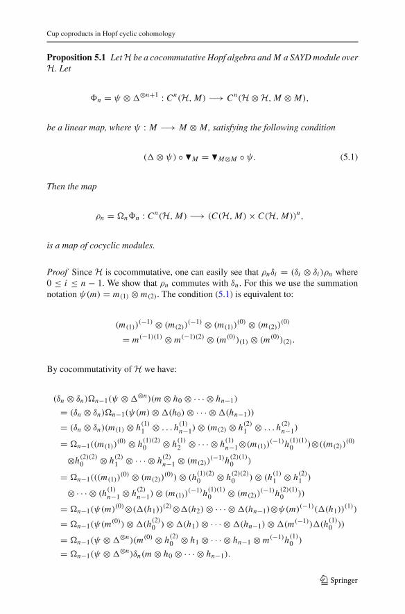
Proposition 5.1 Let H be a cocommutative Hopf algebra and M a SAYD module overH. Let
n = ψ ⊗⊗n+1 : Cn(H,M) −→ Cn(H⊗H,M ⊗ M),
be a linear map, where ψ : M −→ M ⊗ M, satisfying the following condition
(⊗ ψ) ◦ �M = �M⊗M ◦ ψ. (5.1)
Then the map
ρn = �n n : Cn(H,M) −→ (C(H,M)× C(H,M))n,
is a map of cocyclic modules.
Proof Since H is cocommutative, one can easily see that ρnδi = (δi ⊗ δi )ρn where0 ≤ i ≤ n − 1. We show that ρn commutes with δn . For this we use the summationnotation ψ(m) = m(1) ⊗ m(2). The condition (5.1) is equivalent to:
(m(1))(−1) ⊗ (m(2))
(−1) ⊗ (m(1))(0) ⊗ (m(2))
(0)
= m(−1)(1) ⊗ m(−1)(2) ⊗ (m(0))(1) ⊗ (m(0))(2).
By cocommutativity of H we have:
(δn ⊗ δn)�n−1(ψ ⊗⊗n)(m ⊗ h0 ⊗ · · · ⊗ hn−1)
= (δn ⊗ δn)�n−1(ψ(m)⊗(h0)⊗ · · · ⊗(hn−1))
= (δn ⊗ δn)(m(1) ⊗ h(1)1 ⊗ . . . h(1)n−1)⊗ (m(2) ⊗ h(2)1 ⊗ . . . h(2)n−1)
= �n−1((m(1))(0) ⊗ h(1)(2)0 ⊗ h(1)2 ⊗ · · · ⊗ h(1)n−1⊗(m(1))
(−1)h(1)(1)0 )⊗((m(2))(0)
⊗h(2)(2)0 ⊗ h(2)1 ⊗ · · · ⊗ h(2)n−1 ⊗ (m(2))(−1)h(2)(1)0 )
= �n−1(((m(1))(0) ⊗ (m(2))
(0))⊗ (h(1)(2)0 ⊗ h(2)(2)0 )⊗ (h(1)1 ⊗ h(2)1 )
⊗ · · · ⊗ (h(1)n−1 ⊗ h(2)n−1)⊗ (m(1))(−1)h(1)(1)0 ⊗ (m(2))
(−1)h(2)(1)0 ))
= �n−1(ψ(m)(0)⊗((h1))
(2)⊗(h2)⊗ · · · ⊗(hn−1)⊗ψ(m)(−1)((h1))(1))
= �n−1(ψ(m(0))⊗(h(2)0 )⊗(h1)⊗ · · · ⊗(hn−1)⊗(m(−1))(h(1)0 ))
= �n−1(ψ ⊗⊗n)(m(0) ⊗ h(2)0 ⊗ h1 ⊗ · · · ⊗ hn−1 ⊗ m(−1)h(1)0 )
= �n−1(ψ ⊗⊗n)δn(m ⊗ h0 ⊗ · · · ⊗ hn−1).
123
M. Hassanzadeh, M. Khalkhali
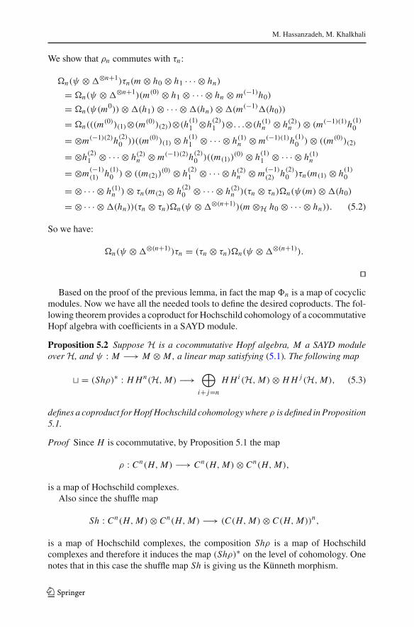
We show that ρn commutes with τn :
�n(ψ ⊗⊗n+1)τn(m ⊗ h0 ⊗ h1 · · · ⊗ hn)
= �n(ψ ⊗⊗n+1)(m(0) ⊗ h1 ⊗ · · · ⊗ hn ⊗ m(−1)h0)
= �n(ψ(m0))⊗(h1)⊗ · · · ⊗(hn)⊗(m(−1)(h0))
= �n(((m(0))(1)⊗(m(0))(2))⊗(h(1)1 ⊗h(2)1 )⊗. . .⊗(h(1)n ⊗ h(2)n )⊗ (m(−1)(1)h(1)0
= ⊗m(−1)(2)h(2)0 ))((m(0))(1) ⊗ h(1)1 ⊗ · · · ⊗ h(1)n ⊗ m(−1)(1)h(1)0 )⊗ ((m(0))(2)
= ⊗h(2)1 ⊗ · · · ⊗ h(2)n ⊗ m(−1)(2)h(2)0 )((m(1))(0) ⊗ h(1)1 ⊗ · · · ⊗ h(1)n
= ⊗m(−1)(1) h(1)0 )⊗ ((m(2))
(0) ⊗ h(2)1 ⊗ · · · ⊗ h(2)n ⊗ m(−1)(2) h(2)0 )τn(m(1) ⊗ h(1)0
= ⊗ · · · ⊗ h(1)n )⊗ τn(m(2) ⊗ h(2)0 ⊗ · · · ⊗ h(2)n )(τn ⊗ τn)�n(ψ(m)⊗(h0)
= ⊗ · · · ⊗(hn))(τn ⊗ τn)�n(ψ ⊗⊗(n+1))(m ⊗H h0 ⊗ · · · ⊗ hn)). (5.2)
So we have:
�n(ψ ⊗⊗(n+1))τn = (τn ⊗ τn)�n(ψ ⊗⊗(n+1)).
��Based on the proof of the previous lemma, in fact the map n is a map of cocyclic
modules. Now we have all the needed tools to define the desired coproducts. The fol-lowing theorem provides a coproduct for Hochschild cohomology of a cocommutativeHopf algebra with coefficients in a SAYD module.
Proposition 5.2 Suppose H is a cocommutative Hopf algebra, M a SAYD moduleover H, and ψ : M −→ M ⊗ M, a linear map satisfying (5.1). The following map
� = (Shρ)∗ : H Hn(H,M) −→⊕
i+ j=n
H Hi (H,M)⊗ H H j (H,M), (5.3)
defines a coproduct for Hopf Hochschild cohomology where ρ is defined in Proposition5.1.
Proof Since H is cocommutative, by Proposition 5.1 the map
ρ : Cn(H,M) −→ Cn(H,M)⊗ Cn(H,M),
is a map of Hochschild complexes.Also since the shuffle map
Sh : Cn(H,M)⊗ Cn(H,M) −→ (C(H,M)⊗ C(H,M))n,
is a map of Hochschild complexes, the composition Shρ is a map of Hochschildcomplexes and therefore it induces the map (Shρ)∗ on the level of cohomology. Onenotes that in this case the shuffle map Sh is giving us the Künneth morphism.
123
Cup coproducts in Hopf cyclic cohomology
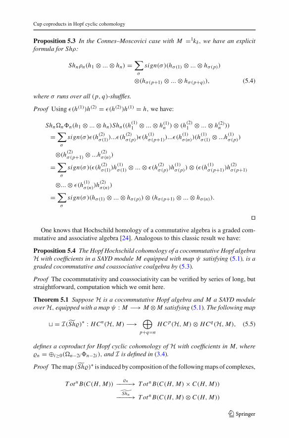
Proposition 5.3 In the Connes–Moscovici case with M =1kδ, we have an explicitformula for Shρ:
Shnρn(h1 ⊗ ...⊗ hn) =∑
σ
sign(σ )(hσ(1) ⊗ ...⊗ hσ(p))
⊗(hσ(p+1) ⊗ ...⊗ hσ(p+q)), (5.4)
where σ runs over all (p, q)-shuffles.
Proof Using ε(h(1))h(2) = ε(h(2))h(1) = h, we have:
Shn�n n(h1 ⊗ ...⊗ hn)Shn((h(1)1 ⊗ ...⊗ h(1)n )⊗ (h(2)1 ⊗ ...⊗ h(2)n ))
=∑
σ
sign(σ )ε(h(2)σ (1))...ε(h(2)σ (p))ε(h
(1)σ (p+1))...ε(h
(1)σ (n))(h
(1)σ (1) ⊗ ...h(1)σ (p))
⊗(h(2)σ (p+1) ⊗ ...h(2)σ (n))=
∑
σ
sign(σ )(ε(h(2)σ (1))h(1)σ (1) ⊗ ...⊗ ε(h(2)σ (p))h(1)σ (p))⊗ (ε(h(1)σ (p+1))h
(2)σ (p+1)
⊗...⊗ ε(h(1)σ (n))h(2)σ (n))=
∑
σ
sign(σ )(hσ(1) ⊗ ...⊗ hσ(p))⊗ (hσ(p+1) ⊗ ...⊗ hσ(n)).
��One knows that Hochschild homology of a commutative algebra is a graded com-
mutative and associative algebra [24]. Analogous to this classic result we have:
Proposition 5.4 The Hopf Hochschild cohomology of a cocommutative Hopf algebraH with coefficients in a SAYD module M equipped with map ψ satisfying (5.1), is agraded cocommutative and coassociative coalgebra by (5.3).
Proof The cocommutativity and coassociativity can be verified by series of long, butstraightforward, computation which we omit here.
Theorem 5.1 Suppose H is a cocommutative Hopf algebra and M a SAYD moduleover H, equipped with a map ψ : M −→ M⊗M satisfying (5.1). The following map
� = I(Sh�)∗ : HCn(H,M) −→⊕
p+q=n
HC p(H,M)⊗ HCq(H,M), (5.5)
defines a coproduct for Hopf cyclic cohomology of H with coefficients in M, where�n = ⊕i≥0(�n−2i n−2i ), and I is defined in (3.4).
Proof The map (Sh�)∗ is induced by composition of the following maps of complexes,
T otn B(C(H,M))�n−−−−→ T otn B(C(H,M)× C(H,M))
˜Shn−−−−→ T otn B(C(H,M)⊗ C(H,M))
123
M. Hassanzadeh, M. Khalkhali
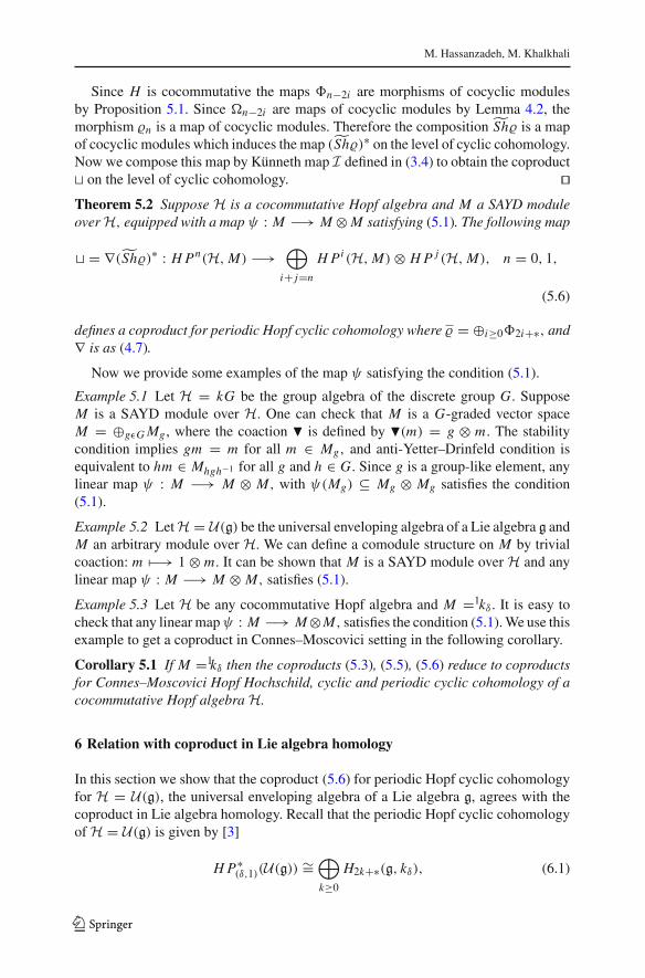
Since H is cocommutative the maps n−2i are morphisms of cocyclic modulesby Proposition 5.1. Since �n−2i are maps of cocyclic modules by Lemma 4.2, themorphism �n is a map of cocyclic modules. Therefore the composition Sh� is a mapof cocyclic modules which induces the map (Sh�)∗ on the level of cyclic cohomology.Now we compose this map by Künneth map I defined in (3.4) to obtain the coproduct� on the level of cyclic cohomology. ��Theorem 5.2 Suppose H is a cocommutative Hopf algebra and M a SAYD moduleover H, equipped with a map ψ : M −→ M⊗M satisfying (5.1). The following map
� = ∇(Sh�)∗ : H Pn(H,M) −→⊕
i+ j=n
H Pi (H,M)⊗ H P j (H,M), n = 0, 1,
(5.6)
defines a coproduct for periodic Hopf cyclic cohomology where � = ⊕i≥0 2i+∗, and∇ is as (4.7).
Now we provide some examples of the map ψ satisfying the condition (5.1).
Example 5.1 Let H = kG be the group algebra of the discrete group G. SupposeM is a SAYD module over H. One can check that M is a G-graded vector spaceM = ⊕gεG Mg , where the coaction � is defined by �(m) = g ⊗ m. The stabilitycondition implies gm = m for all m ∈ Mg, and anti-Yetter–Drinfeld condition isequivalent to hm ∈ Mhgh−1 for all g and h ∈ G. Since g is a group-like element, anylinear map ψ : M −→ M ⊗ M, with ψ(Mg) ⊆ Mg ⊗ Mg satisfies the condition(5.1).
Example 5.2 Let H = U(g) be the universal enveloping algebra of a Lie algebra g andM an arbitrary module over H. We can define a comodule structure on M by trivialcoaction: m −→ 1⊗ m. It can be shown that M is a SAYD module over H and anylinear map ψ : M −→ M ⊗ M, satisfies (5.1).
Example 5.3 Let H be any cocommutative Hopf algebra and M =1kδ . It is easy tocheck that any linear mapψ : M −→ M⊗M, satisfies the condition (5.1). We use thisexample to get a coproduct in Connes–Moscovici setting in the following corollary.
Corollary 5.1 If M =1kδ then the coproducts (5.3), (5.5), (5.6) reduce to coproductsfor Connes–Moscovici Hopf Hochschild, cyclic and periodic cyclic cohomology of acocommutative Hopf algebra H.
6 Relation with coproduct in Lie algebra homology
In this section we show that the coproduct (5.6) for periodic Hopf cyclic cohomologyfor H = U(g), the universal enveloping algebra of a Lie algebra g, agrees with thecoproduct in Lie algebra homology. Recall that the periodic Hopf cyclic cohomologyof H = U(g) is given by [3]
H P∗(δ,1)(U(g)) ∼=⊕
k≥0
H2k+∗(g, kδ), (6.1)
123
Cup coproducts in Hopf cyclic cohomology
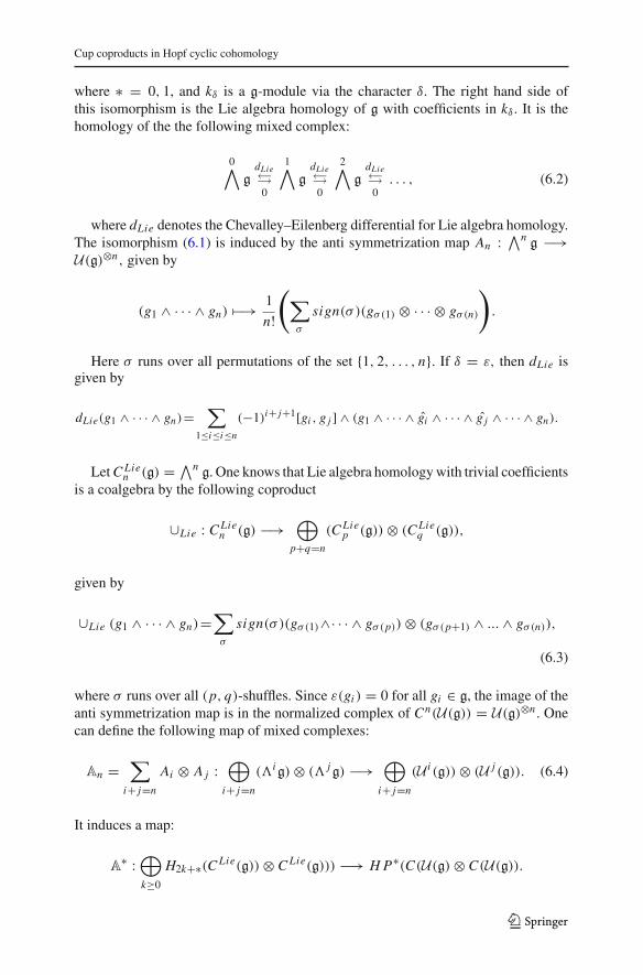
where ∗ = 0, 1, and kδ is a g-module via the character δ. The right hand side ofthis isomorphism is the Lie algebra homology of g with coefficients in kδ . It is thehomology of the the following mixed complex:
0∧g
dLie�0
1∧g
dLie�0
2∧g
dLie�0. . . , (6.2)
where dLie denotes the Chevalley–Eilenberg differential for Lie algebra homology.The isomorphism (6.1) is induced by the anti symmetrization map An : ∧n g −→U(g)⊗n, given by
(g1 ∧ · · · ∧ gn) −→ 1
n!
(∑
σ
sign(σ )(gσ(1) ⊗ · · · ⊗ gσ(n)
)
.
Here σ runs over all permutations of the set {1, 2, . . . , n}. If δ = ε, then dLie isgiven by
dLie(g1 ∧ · · · ∧ gn)=∑
1≤i≤i≤n
(−1)i+ j+1[gi , g j ] ∧ (g1 ∧ · · · ∧ gi ∧ · · · ∧ g j ∧ · · · ∧ gn).
Let C Lien (g) =∧n g. One knows that Lie algebra homology with trivial coefficients
is a coalgebra by the following coproduct
∪Lie : C Lien (g) −→
⊕
p+q=n
(C Liep (g))⊗ (C Lie
q (g)),
given by
∪Lie (g1 ∧ · · · ∧ gn)=∑
σ
sign(σ )(gσ(1)∧· · · ∧ gσ(p))⊗ (gσ(p+1) ∧ ... ∧ gσ(n)),
(6.3)
where σ runs over all (p, q)-shuffles. Since ε(gi ) = 0 for all gi ∈ g, the image of theanti symmetrization map is in the normalized complex of Cn(U(g)) = U(g)⊗n . Onecan define the following map of mixed complexes:
An =∑
i+ j=n
Ai ⊗ A j :⊕
i+ j=n
(�ig)⊗ (� jg) −→⊕
i+ j=n
(U i (g))⊗ (U j (g)). (6.4)
It induces a map:
A∗ :
⊕
k≥0
H2k+∗(C Lie(g))⊗ C Lie(g))) −→ H P∗(C(U(g)⊗ C(U(g)).
123
M. Hassanzadeh, M. Khalkhali
Now using the Künneth formula (4.7), we obtain the following map:
∇(A∪Lie)∗ :
⊕
n≥0
H2n+1(g, kε) −→ H P1(ε,1)(U(g))⊗ H P0
(ε,1)(U(g))
⊕H P0(ε,1)(U(g))⊗ H P1
(ε,1)(U(g)),
and similarly for the even case.
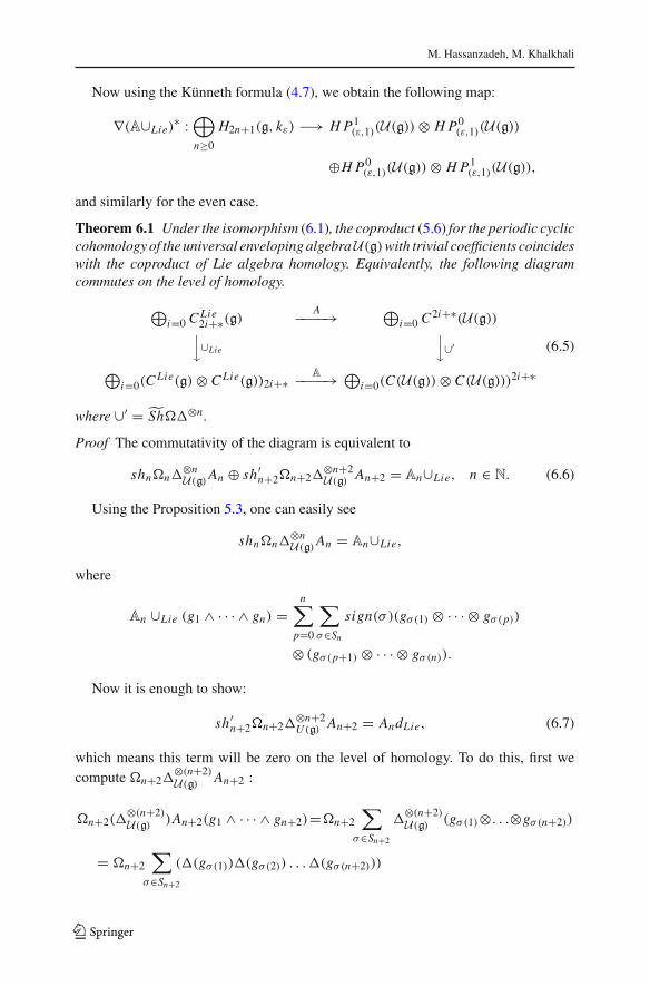
Theorem 6.1 Under the isomorphism (6.1), the coproduct (5.6) for the periodic cycliccohomology of the universal enveloping algebraU(g)with trivial coefficients coincideswith the coproduct of Lie algebra homology. Equivalently, the following diagramcommutes on the level of homology.
⊕i=0 C Lie
2i+∗(g)A−−−−→ ⊕
i=0 C2i+∗(U(g))⏐⏐�∪Lie
⏐⏐�∪′
⊕i=0(C
Lie(g)⊗ C Lie(g))2i+∗A−−−−→ ⊕
i=0(C(U(g))⊗ C(U(g)))2i+∗
(6.5)
where ∪′ = Sh�⊗n.
Proof The commutativity of the diagram is equivalent to
shn�n⊗nU(g)An ⊕ sh′n+2�n+2
⊗n+2U(g) An+2 = An∪Lie, n ∈ N. (6.6)
Using the Proposition 5.3, one can easily see
shn�n⊗nU(g)An = An∪Lie,
where
An ∪Lie (g1 ∧ · · · ∧ gn) =n∑
p=0
∑
σ∈Sn
sign(σ )(gσ(1) ⊗ · · · ⊗ gσ(p))
⊗ (gσ(p+1) ⊗ · · · ⊗ gσ(n)).
Now it is enough to show:
sh′n+2�n+2⊗n+2U (g) An+2 = AndLie, (6.7)
which means this term will be zero on the level of homology. To do this, first wecompute �n+2
⊗(n+2)U(g) An+2 :
�n+2(⊗(n+2)U(g) )An+2(g1 ∧ · · · ∧ gn+2)=�n+2
∑
σ∈Sn+2
⊗(n+2)U(g) (gσ(1)⊗. . .⊗gσ(n+2))
= �n+2
∑
σ∈Sn+2
((gσ(1))(gσ(2)) . . . (gσ(n+2)))
123
Cup coproducts in Hopf cyclic cohomology
= �n+2
∑
σ∈Sn+2
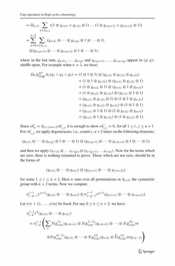
((1⊗ gσ(1) + gσ(1) ⊗ 1) . . . (1⊗ gσ(n+2) + gσ(n+2) ⊗ 1))
=n+2∑
p=0
∑
σ∈Sn+2
(gσ(1) ⊗ · · · ⊗ gσ(p) ⊗ 1⊗ · · · ⊗ 1)
⊗(gσ(p+1) ⊗ · · · ⊗ gσ(n+2) ⊗ 1⊗ · · · ⊗ 1),
where in the last sum, gσ(1), . . . , gσ(p) and gσ(p+1), . . . , gσ(p+q) appear in (p, q)-shuffle spots. For example when n = 1, we have:
�3⊗3U(g)A3(g1 ∧ g2 ∧ g3) = (1⊗ 1⊗ 1)⊗ (gσ(1) ⊗ gσ(2) ⊗ gσ(3))
+ (1⊗ 1⊗ gσ(3))⊗ (gσ(1) ⊗ gσ(2) ⊗ 1)
+ (1⊗ gσ(2) ⊗ 1)⊗ (gσ(1) ⊗ 1⊗ gσ(3))
+ (1⊗ gσ(2) ⊗ gσ(3))⊗ (gσ(1) ⊗ 1⊗ 1)
+ (gσ(1) ⊗ gσ(2) ⊗ 1)⊗ (1⊗ 1⊗ gσ(3))
+ (gσ(1) ⊗ gσ(2) ⊗ gσ(3))⊗ (1⊗ 1⊗ 1)
+ (gσ(1) ⊗ 1⊗ 1)⊗ (1⊗ gσ(2) ⊗ gσ(3))
+ (gσ(1) ⊗ 1⊗ gσ(3))⊗ (1⊗ gσ(2) ⊗ 1).
Since sh′n = ⊕i+ j=n+2sh′i, j , it is enough to show sh′i, j = 0, for all 1 ≤ i, j ≤ n+ 1.For sh′i, j , we apply degeneracies, i.e., counit ε, n+2 times on the following elements:
(gσ(1) ⊗ · · · ⊗ gσ(p) ⊗ 1⊗ · · · ⊗ 1)⊗ (gσ(p+1) ⊗ · · · ⊗ gσ(n+2) ⊗ 1⊗ · · · ⊗ 1),
and then we apply (sσ ′(1)⊗ . . . sσ ′(q))⊗ (sσ ′(q+1) . . . sσ ′(n)). Now for the terms whichare zero, there is nothing remained to prove. Those which are not zero, should be inthe forms of
(gσ(1) ⊗ · · · ⊗ gσ(i))⊗ (gσ(i+1) ⊗ · · · ⊗ gσ(n+2)),
for some 1 ≤ i ≤ n + 2. Here σ runs over all permutations in Sn+2, the symmetricgroup with n + 2 terms. Now we compute
σ i−1i−p−1τ
p+1(gσ(1) ⊗ · · · ⊗ gσ(i))⊗ σ j−1j−q−1τ
q+1(gσ(i+1) ⊗ · · · ⊗ gσ(n+2)).
Let σ(i + 1), . . . , σ (n) be fixed. For any 0 ≤ k ≤ n + 2, we have:
σ i−1i−k τ
k(gσ(1) ⊗ · · · ⊗ gσ(i))
= σ i−1i−k
(∑
σ
S(g(i)σ (k))gσ(k+1) ⊗ S(g(i−1)σ (k) )gσ(k+2) ⊗ · · · ⊗ S(g(k)σ (k))σ
⊗S(g(k−1)σ (k) )gσ(1) ⊗ · · · ⊗ S(g(2)σ (k))gσ(2) ⊗ S(g(1)σ (k))σgσ(i−1)
)
123
M. Hassanzadeh, M. Khalkhali
= σ i−1i−k
⎛
⎝∑
σ∈Sp
i−1∑
r=k+1
gσ(k+1) ⊗ . . . gσ(r−1)
⊗gσ(k)gσ(r) ⊗ gσ(r+1) ⊗ · · · ⊗ gσ(i) ⊗ 1⊗ gσ(1) ⊗ · · · ⊗ gσ(i−1)
+ gσ(k+1) ⊗ · · · ⊗ gσ(i) ⊗ gσ(k) ⊗ gσ(1) ⊗ · · · ⊗ gσ(i−1)
⎞
⎠
=∑
σ∈Si
p−1∑
r=k+1
gσ(k+1) ⊗ · · · ⊗ gσ(r−1)
⊗gσ(k)gσ(r) ⊗ gσ(r+1) ⊗ · · · ⊗ gσ(i) ⊗ gσ(1) ⊗ · · · ⊗ gσ(i−1)
=∑
σ∈Si ,σ (v)>σ(w)
gσ(1) ⊗ · · · ⊗ gσ(v)gσ(w) ⊗ · · · ⊗ gσ(i)
+∑
σ∈Si ,σ (v)>σ(w)
gσ(1) ⊗ · · · ⊗ gσ(w)gσ(v) ⊗ · · · ⊗ gσ(i)
=∑
σ∈Si ,σ (v)>σ(w)
gσ(1) ⊗ · · · ⊗ gσ(v)gσ(w) − gσ(w)gσ(v) ⊗ · · · ⊗ gσ(i)
=∑
σ∈Si ,σ (v)>σ(w)
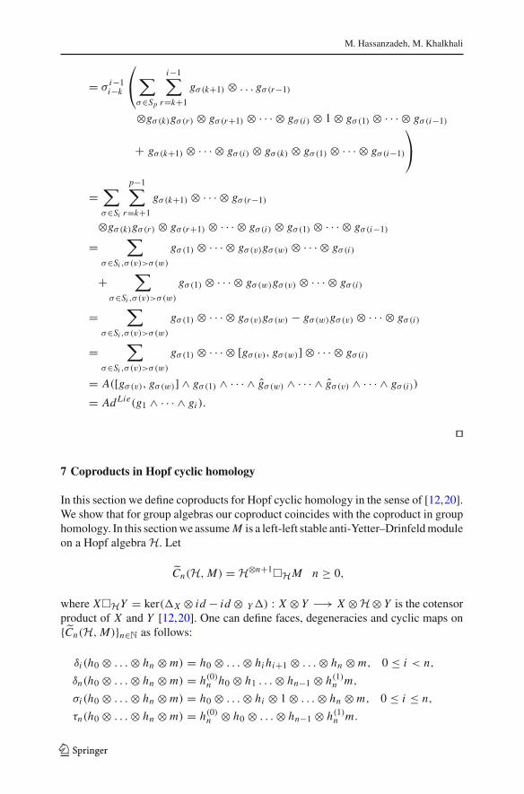
gσ(1) ⊗ · · · ⊗ [gσ(v), gσ(w)] ⊗ · · · ⊗ gσ(i)
= A([gσ(v), gσ(w)] ∧ gσ(1) ∧ · · · ∧ gσ(w) ∧ · · · ∧ gσ(v) ∧ · · · ∧ gσ(i))
= Ad Lie(g1 ∧ · · · ∧ gi ).
��
7 Coproducts in Hopf cyclic homology
In this section we define coproducts for Hopf cyclic homology in the sense of [12,20].We show that for group algebras our coproduct coincides with the coproduct in grouphomology. In this section we assume M is a left-left stable anti-Yetter–Drinfeld moduleon a Hopf algebra H. Let
Cn(H,M) = H⊗n+1�HM n ≥ 0,
where X�HY = ker(X ⊗ id − id ⊗ Y) : X ⊗ Y −→ X ⊗H⊗ Y is the cotensorproduct of X and Y [12,20]. One can define faces, degeneracies and cyclic maps on{Cn(H,M)}n∈N as follows:
δi (h0 ⊗ . . .⊗ hn ⊗ m) = h0 ⊗ . . .⊗ hi hi+1 ⊗ . . .⊗ hn ⊗ m, 0 ≤ i < n,
δn(h0 ⊗ . . .⊗ hn ⊗ m) = h(0)n h0 ⊗ h1 . . .⊗ hn−1 ⊗ h(1)n m,
σi (h0 ⊗ . . .⊗ hn ⊗ m) = h0 ⊗ . . .⊗ hi ⊗ 1⊗ . . .⊗ hn ⊗ m, 0 ≤ i ≤ n,
τn(h0 ⊗ . . .⊗ hn ⊗ m) = h(0)n ⊗ h0 ⊗ . . .⊗ hn−1 ⊗ h(1)n m.
123
Cup coproducts in Hopf cyclic cohomology
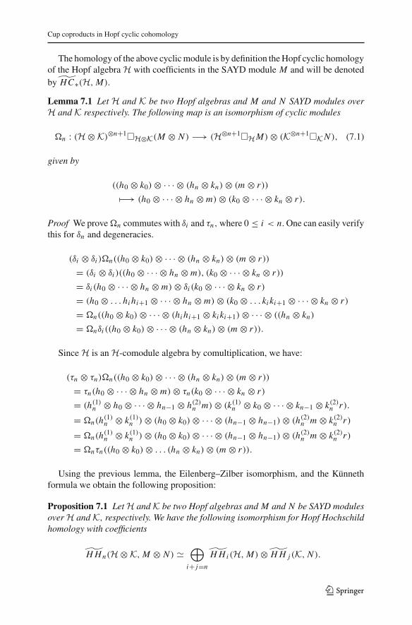
The homology of the above cyclic module is by definition the Hopf cyclic homologyof the Hopf algebra H with coefficients in the SAYD module M and will be denotedby HC∗(H,M).
Lemma 7.1 Let H and K be two Hopf algebras and M and N SAYD modules overH and K respectively. The following map is an isomorphism of cyclic modules
�n : (H⊗K)⊗n+1�H⊗K(M ⊗ N ) −→ (H⊗n+1�HM)⊗ (K⊗n+1�KN ), (7.1)
given by
((h0 ⊗ k0)⊗ · · · ⊗ (hn ⊗ kn)⊗ (m ⊗ r))
−→ (h0 ⊗ · · · ⊗ hn ⊗ m)⊗ (k0 ⊗ · · · ⊗ kn ⊗ r).
Proof We prove�n commutes with δi and τn,where 0 ≤ i < n. One can easily verifythis for δn and degeneracies.
(δi ⊗ δi )�n((h0 ⊗ k0)⊗ · · · ⊗ (hn ⊗ kn)⊗ (m ⊗ r))
= (δi ⊗ δi )((h0 ⊗ · · · ⊗ hn ⊗ m), (k0 ⊗ · · · ⊗ kn ⊗ r))
= δi (h0 ⊗ · · · ⊗ hn ⊗ m)⊗ δi (k0 ⊗ · · · ⊗ kn ⊗ r)
= (h0 ⊗ . . . hi hi+1 ⊗ · · · ⊗ hn ⊗ m)⊗ (k0 ⊗ . . . ki ki+1 ⊗ · · · ⊗ kn ⊗ r)
= �n((h0 ⊗ k0)⊗ · · · ⊗ (hi hi+1 ⊗ ki ki+1)⊗ · · · ⊗ ((hn ⊗ kn)
= �nδi ((h0 ⊗ k0)⊗ · · · ⊗ (hn ⊗ kn)⊗ (m ⊗ r)).
Since H is an H-comodule algebra by comultiplication, we have:
(τn ⊗ τn)�n((h0 ⊗ k0)⊗ · · · ⊗ (hn ⊗ kn)⊗ (m ⊗ r))
= τn(h0 ⊗ · · · ⊗ hn ⊗ m)⊗ τn(k0 ⊗ · · · ⊗ kn ⊗ r)
= (h(1)n ⊗ h0 ⊗ · · · ⊗ hn−1 ⊗ h(2)n m)⊗ (k(1)n ⊗ k0 ⊗ · · · ⊗ kn−1 ⊗ k(2)n r).
= �n(h(1)n ⊗ k(1)n )⊗ (h0 ⊗ k0)⊗ · · · ⊗ (hn−1 ⊗ hn−1)⊗ (h(2)n m ⊗ k(2)n r)
= �n(h(1)n ⊗ k(1)n )⊗ (h0 ⊗ k0)⊗ · · · ⊗ (hn−1 ⊗ hn−1)⊗ (h(2)n m ⊗ k(2)n r)
= �nτn((h0 ⊗ k0)⊗ . . . (hn ⊗ kn)⊗ (m ⊗ r)).
Using the previous lemma, the Eilenberg–Zilber isomorphism, and the Künnethformula we obtain the following proposition:
Proposition 7.1 Let H and K be two Hopf algebras and M and N be SAYD modulesover H and K, respectively. We have the following isomorphism for Hopf Hochschildhomology with coefficients
H Hn(H⊗K,M ⊗ N ) �⊕
i+ j=n
H Hi (H,M)⊗ H H j (K, N ).
123
M. Hassanzadeh, M. Khalkhali
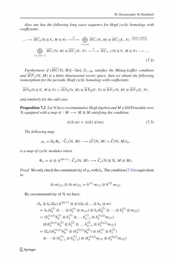
Also one has the following long exact sequence for Hopf cyclic homology withcoefficients:
... −→ HCn(H⊗K,M ⊗ N )I−−−−−→
⊕
i+ j=n
HCi (H,M)⊗ HC j (K, N )S⊗id−id⊗S−−−−−−−→
⊕
i+ j=n−2
HCi (H,M)⊗ HC j (K, N )∂−−−−−→ HCn−1(H⊗K,M ⊗ N ) −→ ....
(7.2)
Furthermore if (HC(H,M)[−2m], S)−2m satisfies the Mittag-Leffler conditionand H P∗(H,M) is a finite dimensional vector space, then we obtain the followingisomorphism for the periodic Hopf cyclic homology with coefficients:
H P0(H⊗K,M ⊗ N ) � H P0(H,M)⊗ H P0(K, N )⊕ H P1(H,M)⊗ H P1(K, N ),
and similarly for the odd case.
Proposition 7.2 Let H be a cocommutative Hopf algebra and M a SAYD module overH equipped with a map ψ : M −→ M ⊗ M satisfying the condition:
ψ(h.m) = (h).ψ(m). (7.3)
The following map
ρn = �n n : Cn(H,M) −→ (C(H,M)× C(H,M))n,
is a map of cyclic modules where
n = ψ ⊗⊗n+1 : Cn(H,M) −→ Cn(H⊗H,M ⊗ M).
Proof We only check the commutativity ofρn with δn . The condition (7.3) is equivalentto
(h.m)(1) ⊗ (h.m)(2) = h(1).m(1) ⊗ h(2).m(2).
By cocommutativity of H we have:
(δn ⊗ δn)�n(⊗n+1 ⊗ ψ)(h0 ⊗ ...⊗ hn ⊗ m)
= δn(h(1)0 ⊗ · · · ⊗ h(1)n ⊗ m(1))⊗ δn(h
(2)0 ⊗ · · · ⊗ h(2)n ⊗ m(2))
= (h(1)(1)n h(1)0 ⊗ h(1)1 ⊗ . . . h(1)n−1 ⊗ h(1)(2)n m(1))
⊗(h(2)(1)n h(2)0 ⊗ h(2)1 ⊗ . . . h(2)n−1 ⊗ h(2)(2)n m(2))
= �n((h(1)(1)n h(1)0 ⊗ (h(2)(1)n h(2)0 )⊗ (h(1)1 ⊗ h(2)1 )
⊗ · · · ⊗ (h(1)n−1 ⊗ h(2)n−1)⊗ (h(1)(2)n m(1) ⊗ h(2)(2)n m(2))
123
Cup coproducts in Hopf cyclic cohomology
= �n((h(1)(1)n h(1)0 ⊗ (h(1)(2)n h(2)0 )⊗ (h(1)1 ⊗ h(2)1 )
⊗ · · · ⊗ (h(1)n−1 ⊗ h(2)n−1)⊗ (h(2)n m)(1) ⊗ (h(2)n m)(2))
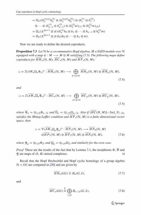
= �n(⊗n+1 ⊗ ψ)(h(1)n h0 ⊗ h1 ⊗ · · · ⊗ hn−1 ⊗ h(2)n m)
= �n(⊗n+1 ⊗ ψ)δn(h0 ⊗ · · · ⊗ hn ⊗ m).
Now we are ready to define the desired coproducts.
Proposition 7.3 Let H be a cocommutative Hopf algebra, M a SAYD module over Hequipped with a map ψ : M −→ M ⊗ M satisfying (7.3). The following maps definecoproducts for H H∗(H,M), HC∗(H,M) and H P∗(H,M):
� = I(AWn�n n)∗ : H Hn(H,M) −→
⊕
p+q=n
H H p(H,M)⊗ H Hq(H,M),
(7.4)
and
� = I (AW n�n n)∗ : HCn(H,M) −→
⊕
p+q=n
HC p(H,M)⊗ HCq(H,M),
(7.5)
where n = ⊕i≥0 n−2i and �n = ⊕i≥0�n−2i . Also if (HC(H,M)[−2m], S)−2m
satisfies the Mittag-Leffler condition and H P∗(H,M) is a finite dimensional vectorspace, then
� = ∇ (AW n�n n)∗ : H P1(H,M) −→ H P0(H,M)
⊗H P1(H,M)⊕ H P1(H,M)⊗ H P0(H,M), (7.6)
where n = ⊕i≥0 2i and �n = ⊕i≥0�2i and similarly for the even case.
Proof These are the results of the fact that by Lemma 7.1, the morphisms , and are maps of (b, B)-mixed complexes. ��
Recall that the Hopf Hochschild and Hopf cyclic homology of a group algebraH = kG are computed in [20] and are given by
H Hn(kG) ∼= Hn(G, k), (7.7)
and
HCn(kG)θ∼=
⊕
i≥0
Hn−2i (G, k), (7.8)
123
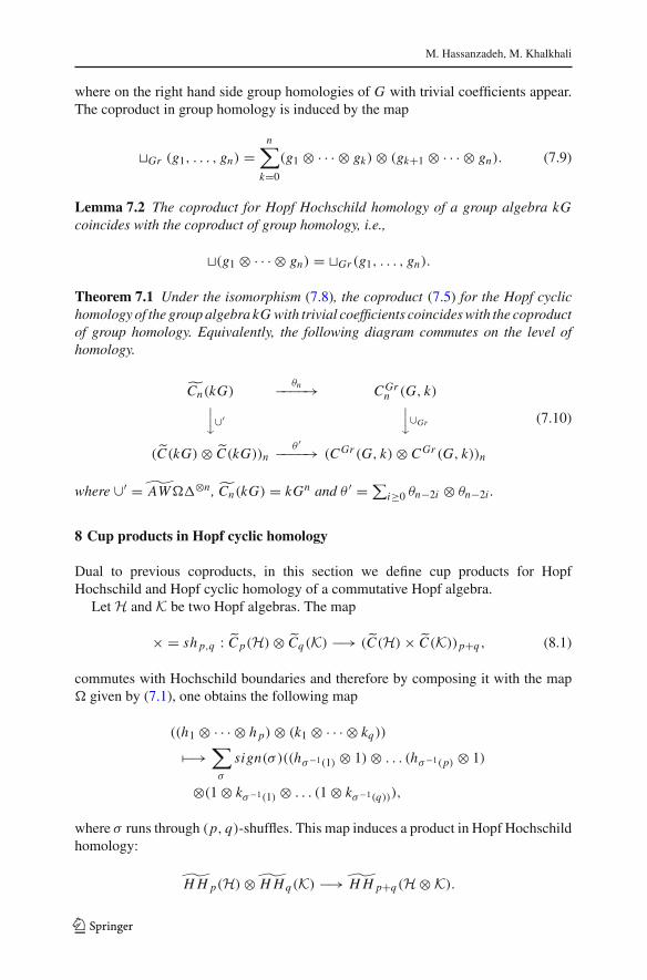
M. Hassanzadeh, M. Khalkhali
where on the right hand side group homologies of G with trivial coefficients appear.The coproduct in group homology is induced by the map
�Gr (g1, . . . , gn) =n∑
k=0
(g1 ⊗ · · · ⊗ gk)⊗ (gk+1 ⊗ · · · ⊗ gn). (7.9)
Lemma 7.2 The coproduct for Hopf Hochschild homology of a group algebra kGcoincides with the coproduct of group homology, i.e.,
�(g1 ⊗ · · · ⊗ gn) = �Gr (g1, . . . , gn).
Theorem 7.1 Under the isomorphism (7.8), the coproduct (7.5) for the Hopf cyclichomology of the group algebra kG with trivial coefficients coincides with the coproductof group homology. Equivalently, the following diagram commutes on the level ofhomology.
Cn(kG)θn−−−−→ CGr
n (G, k)⏐⏐�∪′
⏐⏐�∪Gr
(C(kG)⊗ C(kG))nθ ′−−−−→ (CGr (G, k)⊗ CGr (G, k))n
(7.10)
where ∪′ = AW�⊗n, Cn(kG) = kGn and θ ′ =∑i≥0 θn−2i ⊗ θn−2i .
8 Cup products in Hopf cyclic homology
Dual to previous coproducts, in this section we define cup products for HopfHochschild and Hopf cyclic homology of a commutative Hopf algebra.
Let H and K be two Hopf algebras. The map
× = sh p,q : C p(H)⊗ Cq(K) −→ (C(H)× C(K))p+q , (8.1)
commutes with Hochschild boundaries and therefore by composing it with the map� given by (7.1), one obtains the following map
((h1 ⊗ · · · ⊗ h p)⊗ (k1 ⊗ · · · ⊗ kq))
−→∑
σ
sign(σ )((hσ−1(1) ⊗ 1)⊗ . . . (hσ−1(p) ⊗ 1)
⊗(1⊗ kσ−1(1) ⊗ . . . (1⊗ kσ−1(q))),
where σ runs through (p, q)-shuffles. This map induces a product in Hopf Hochschildhomology:
H H p(H)⊗ H Hq(K) −→ H H p+q(H⊗K).
123
Cup coproducts in Hopf cyclic cohomology
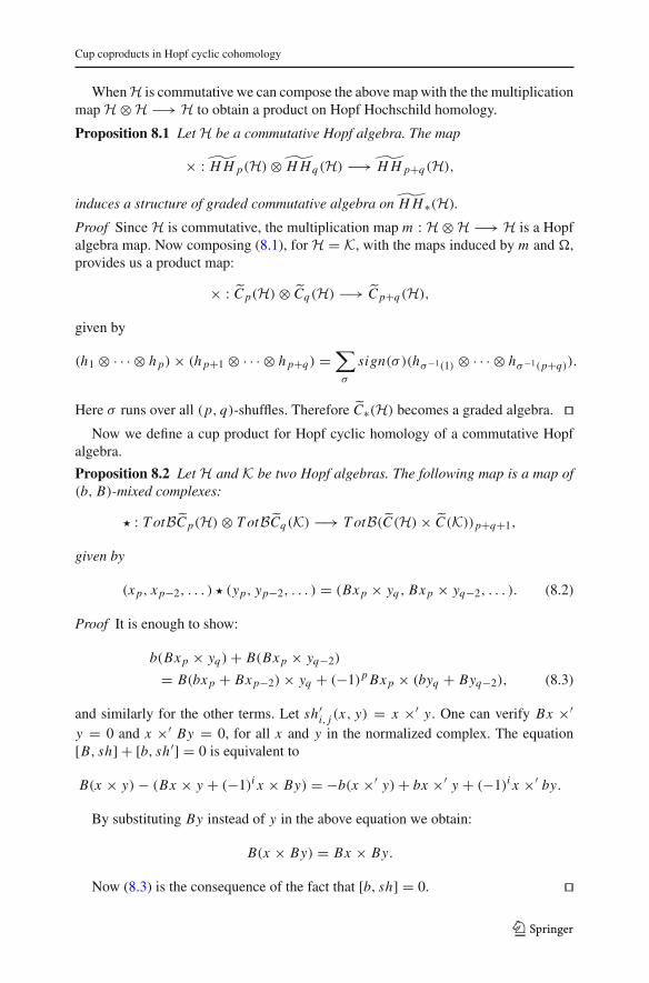
When H is commutative we can compose the above map with the the multiplicationmap H⊗H −→ H to obtain a product on Hopf Hochschild homology.
Proposition 8.1 Let H be a commutative Hopf algebra. The map
× : H H p(H)⊗ H Hq(H) −→ H H p+q(H),
induces a structure of graded commutative algebra on H H∗(H).Proof Since H is commutative, the multiplication map m : H⊗H −→ H is a Hopfalgebra map. Now composing (8.1), for H = K, with the maps induced by m and �,provides us a product map:
× : C p(H)⊗ Cq(H) −→ C p+q(H),
given by
(h1 ⊗ · · · ⊗ h p)× (h p+1 ⊗ · · · ⊗ h p+q) =∑
σ
sign(σ )(hσ−1(1) ⊗ · · · ⊗ hσ−1(p+q)).
Here σ runs over all (p, q)-shuffles. Therefore C∗(H) becomes a graded algebra. ��Now we define a cup product for Hopf cyclic homology of a commutative Hopf
algebra.
Proposition 8.2 Let H and K be two Hopf algebras. The following map is a map of(b, B)-mixed complexes:
� : T otBC p(H)⊗ T otBCq(K) −→ T otB(C(H)× C(K))p+q+1,
given by
(x p, x p−2, . . . ) � (yp, yp−2, . . . ) = (Bx p × yq , Bx p × yq−2, . . . ). (8.2)
Proof It is enough to show:
b(Bx p × yq)+ B(Bx p × yq−2)
= B(bx p + Bx p−2)× yq + (−1)p Bx p × (byq + Byq−2), (8.3)
and similarly for the other terms. Let sh′i, j (x, y) = x ×′ y. One can verify Bx ×′y = 0 and x ×′ By = 0, for all x and y in the normalized complex. The equation[B, sh] + [b, sh′] = 0 is equivalent to
B(x × y)− (Bx × y + (−1)i x × By) = −b(x ×′ y)+ bx ×′ y + (−1)i x ×′ by.
By substituting By instead of y in the above equation we obtain:
B(x × By) = Bx × By.
Now (8.3) is the consequence of the fact that [b, sh] = 0. ��
123
M. Hassanzadeh, M. Khalkhali
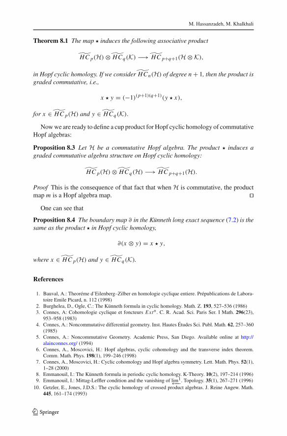
Theorem 8.1 The map � induces the following associative product
HC p(H)⊗ HCq(K) −→ HC p+q+1(H⊗K),
in Hopf cyclic homology. If we consider HCn(H) of degree n+ 1, then the product isgraded commutative, i.e.,
x � y = (−1)(p+1)(q+1)(y � x),
for x ∈ HC p(H) and y ∈ HCq(K).Now we are ready to define a cup product for Hopf cyclic homology of commutative
Hopf algebras:
Proposition 8.3 Let H be a commutative Hopf algebra. The product � induces agraded commutative algebra structure on Hopf cyclic homology:
HC p(H)⊗ HCq(H) −→ HC p+q+1(H).
Proof This is the consequence of that fact that when H is commutative, the productmap m is a Hopf algebra map. ��
One can see that
Proposition 8.4 The boundary map ∂ in the Künneth long exact sequence (7.2) is thesame as the product � in Hopf cyclic homology,
∂(x ⊗ y) = x � y,
where x ∈ HC p(H) and y ∈ HCq(K).
References
1. Bauval, A.: Theoréme d’Eilenberg–Zilber en homologie cyclique entiere. Prépublications de Labora-toire Emile Picard, n. 112 (1998)
2. Burghelea, D., Ogle, C.: The Künneth formula in cyclic homology. Math. Z. 193, 527–536 (1986)3. Connes, A: Cohomologie cyclique et foncteurs Extn . C. R. Acad. Sci. Paris Ser. I Math. 296(23),
953–958 (1983)4. Connes, A.: Noncommutative differential geometry. Inst. Hautes Études Sci. Publ. Math. 62, 257–360
(1985)5. Connes, A.: Noncommutative Geometry. Academic Press, San Diego. Available online at http://
alainconnes.org/ (1994)6. Connes, A., Moscovici, H.: Hopf algebras, cyclic cohomology and the transverse index theorem.
Comm. Math. Phys. 198(1), 199–246 (1998)7. Connes, A., Moscovici, H.: Cyclic cohomology and Hopf algebra symmetry. Lett. Math. Phys. 52(1),
1–28 (2000)8. Emmanouil, I.: The Künneth formula in periodic cyclic homology. K-Theory. 10(2), 197–214 (1996)9. Emmanouil, I.: Mittag-Leffler condition and the vanishing of lim1←−−. Topology. 35(1), 267–271 (1996)
10. Getzler, E., Jones, J.D.S.: The cyclic homology of crossed product algebras. J. Reine Angew. Math.445, 161–174 (1993)
123
Cup coproducts in Hopf cyclic cohomology
11. Gorokhovsky, A.: Secondary characteristic classes and cyclic cohomology of Hopf algebras. Topology.41(5), 993–1016 (2002)
12. Hajac, P.M., Khalkhali, M., Rangipour, B., Sommerhäuser, Y.: Stable anti-Yetter–Drinfeld modules.C. R. Acad. Sci. Paris. 338(8), 587–590 (2004)
13. Hajac, P.M., Khalkhali, M., Rangipour, B., Sommerhäuser, Y.: Hopf-cyclic homology and cohomologywith coefficients. C. R. Acad. Sci. Paris. 338(9), 667–672 (2004)
14. Kaygun, A.: Products in Hopf-cyclic cohomology. Homol. Homotopy Appl. 10(2), 115–133 (2008)15. Kaygun, A.: Uniqueness of pairings in Hopf-cyclic cohomology. J. K-Theory. 6(1), 1–21 (2010)16. Karoubi, M.: Formule de Künneth en homologie cyclique I. (French) [The Künneth formula in cyclic
homology. I] C. R. Acad. Sci. Paris Sèr. I Math. 303(12), 527–530 (1986)17. Karoubi, M.: Formule de Künneth en homologie cyclique II. (French) [The Künneth formula in cyclic
homology. II] C. R. Acad. Sci. Paris Sèr. I Math. 303(13), 595–598 (1986)18. Kassel, C.: Cyclic homology, comodules and mixed complexes. J. Algebra. 107, 195–216 (1987)19. Kassel, C.: A Künneth formula for the cyclic cohomology of Z2-graded algebras. Math. Ann. 275,
683–699 (1986)20. Khalkhali, M. Rangipour, B.: A new cyclic module for Hopf algebras. K -Theory. 27(2), 111–131
(2002)21. Khalkhali, M., Rangipour, B.: On the generalized cyclic Eilenberg–Zilber theorem. Can. Math. Bull.
47(1), 33–48 (2004)22. Khalkhali, M., Rangipour, B.: Cup products in Hopf-cyclic cohomology. C. R. Acad. Sci. Paris. 340(1),
9–14 (2005)23. Kustermans, J., Rognes, J., Tuset, L.: The Connes–Moscovici approach to cyclic cohomology for
compact quantum groups. K-Theory. 26, 101–137 (2002)24. Loday, J.L.: Cyclic homology. Springer, Berlin/Heidelberg/New York (1992)25. Rangipour, B.: Cup products in Hopf cyclic cohomology via cyclic modules. Homol. Homotopy Appl.
10(2), 273–286 (2008)26. Real, P.: Homological perturbation theory and associativity. Homol. Homotopy Appl. 2(5), 51–88
(2000)
123