cumt heat transfer lecture chapter 3 steady-state conduction multiple dimensions chaper 3...
Post on 18-Dec-2015
237 views
TRANSCRIPT
CUMT
HEAT TRANSFER LECTURE
Chapter 3 Steady-State Conduction Multiple Dimensions
CHAPER 3 Steady-State Conduction
Multiple Dimensions
CUMT
HEAT TRANSFER LECTURE
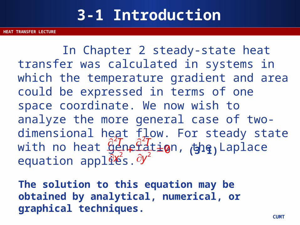
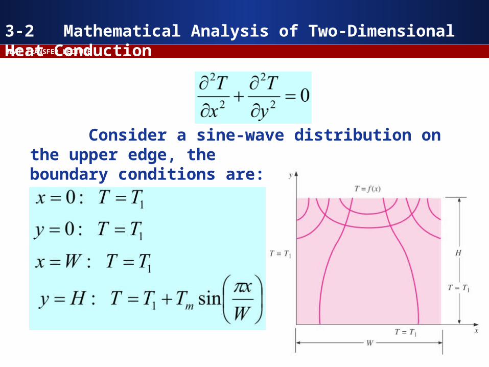
In Chapter 2 steady-state heat transfer was calculated in systems in which the temperature gradient and area could be expressed in terms of one space coordinate. We now wish to analyze the more general case of two-dimensional heat flow. For steady state with no heat generation, the Laplace equation applies.
2 2
2 20
T T
x y
The solution to this equation may be obtained by analytical, numerical, or graphical techniques.
(3-1)
3-1 Introduction
CUMT
HEAT TRANSFER LECTURE
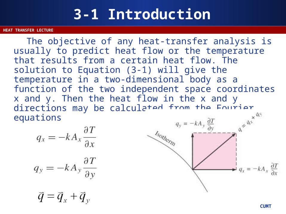
The objective of any heat-transfer analysis is usually to predict heat flow or the temperature that results from a certain heat flow. The solution to Equation (3-1) will give the temperature in a two-dimensional body as a function of the two independent space coordinates x and y. Then the heat flow in the x and y directions may be calculated from the Fourier equations
3-1 Introduction
CUMT
HEAT TRANSFER LECTURE
3-2 Mathematical Analysis of Two-Dimensional Heat Conduction
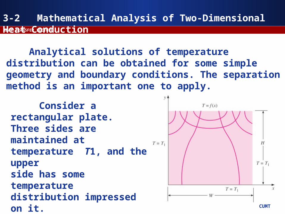
Analytical solutions of temperature distribution can be obtained for some simple geometry and boundary conditions. The separation method is an important one to apply.
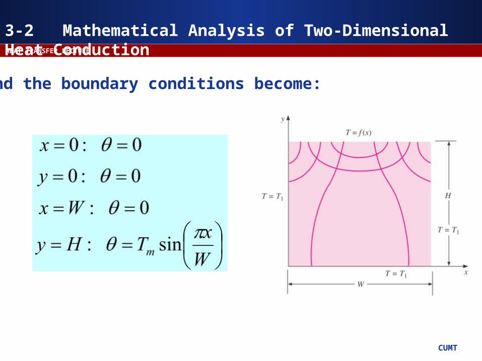
Consider a rectangular plate. Three sides are maintained at temperature T1, and the upper side has some temperature distribution impressed on it.The distribution can be a constant temperature or something more complex, such as a sine-wave.
CUMT
HEAT TRANSFER LECTURE
Consider a sine-wave distribution on the upper edge, the boundary conditions are:
3-2 Mathematical Analysis of Two-Dimensional Heat Conduction
CUMT
HEAT TRANSFER LECTURE
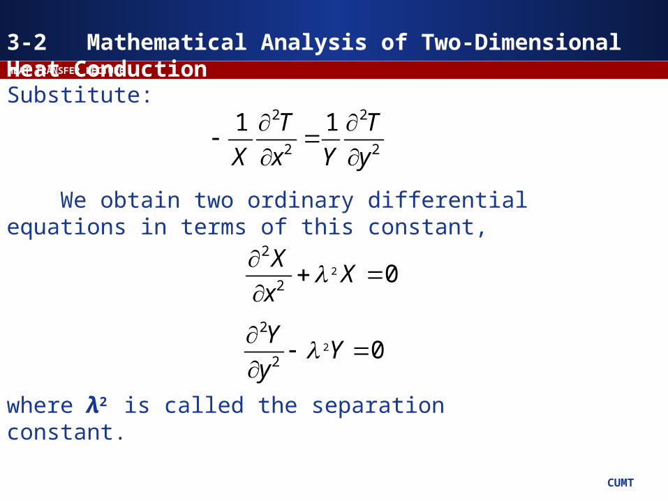
Substitute:
We obtain two ordinary differential equations in terms of this constant,
2 2
2 2
1 1T T
X x Y y
2
2
20
XX
x
2
2
20
YY
y
where λ2 is called the separation constant.
3-2 Mathematical Analysis of Two-Dimensional Heat Conduction
CUMT
HEAT TRANSFER LECTURE
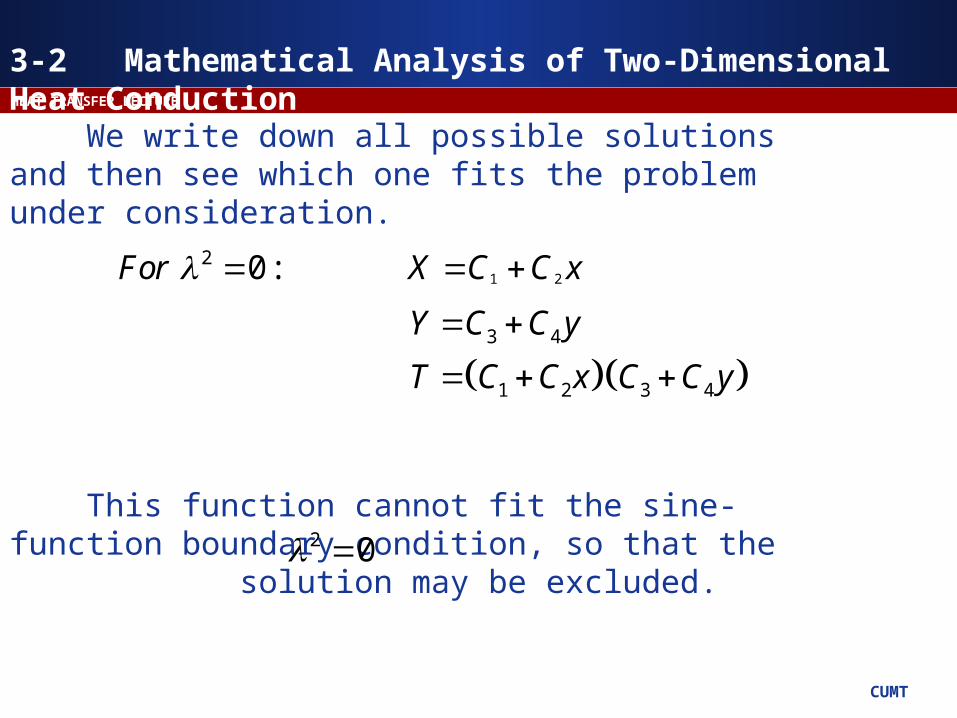
We write down all possible solutions and then see which one fits the problem under consideration.
1 2
2
3 4
1 2 3 4
0 :
For X C C x
Y C C y
T C C x C C y
This function cannot fit the sine-function boundary condition, so that the solution may be excluded.2 0
3-2 Mathematical Analysis of Two-Dimensional Heat Conduction
CUMT
HEAT TRANSFER LECTURE
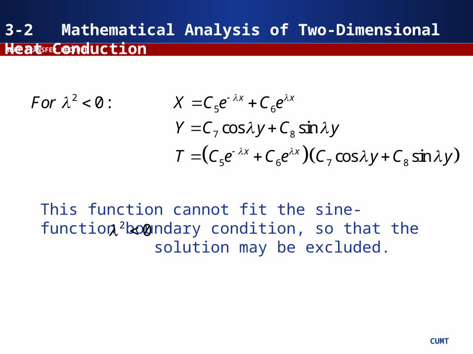
25 6
7 8
5 6 7 8
0 :
cos sin
cos sin
x x
x x
For X C e C e
Y C y C y
T C e C e C y C y
This function cannot fit the sine-function boundary condition, so that the solution may be excluded.2 0
3-2 Mathematical Analysis of Two-Dimensional Heat Conduction
CUMT
HEAT TRANSFER LECTURE
29 10
11 12
9 10 11 12
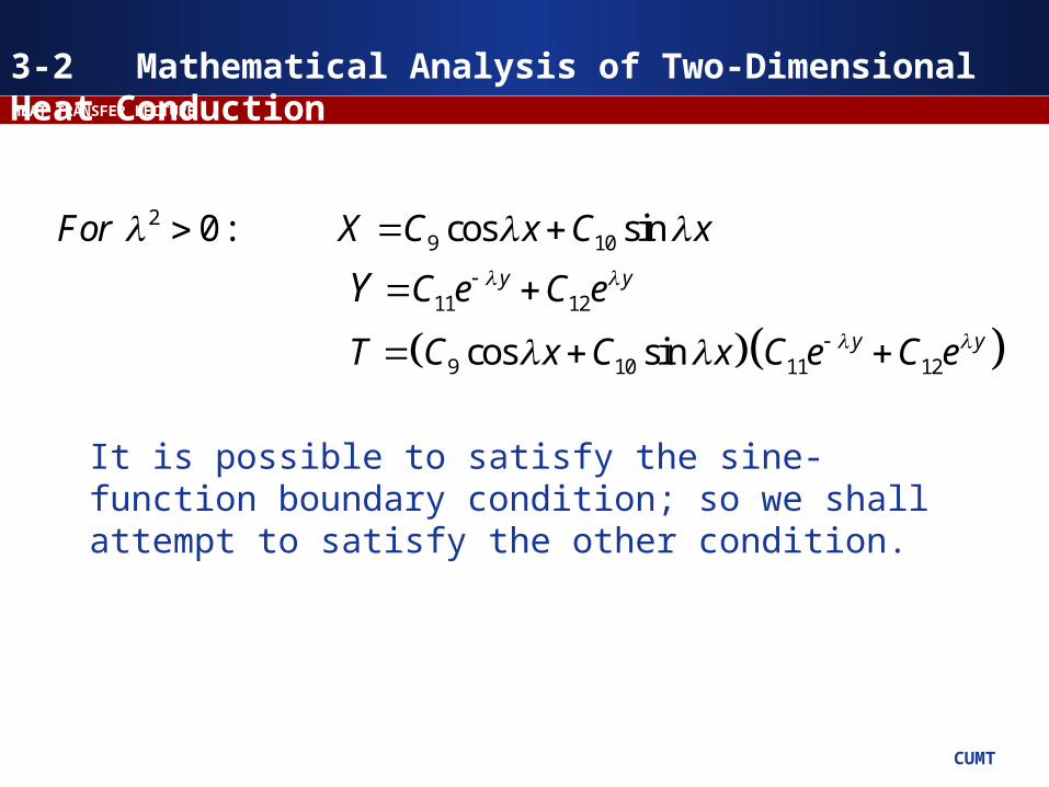
0 : cos sin
cos sin
y y
y y
For X C x C x
C e C e
T C x C x C e C e
Y
It is possible to satisfy the sine-function boundary condition; so we shall attempt to satisfy the other condition.
3-2 Mathematical Analysis of Two-Dimensional Heat Conduction
CUMT
HEAT TRANSFER LECTURE
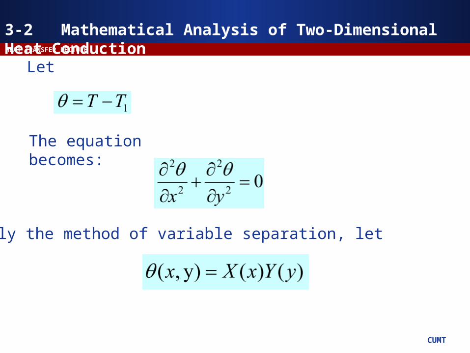
Let
The equation becomes:
Apply the method of variable separation, let
3-2 Mathematical Analysis of Two-Dimensional Heat Conduction
CUMT
HEAT TRANSFER LECTURE
And the boundary conditions become:
3-2 Mathematical Analysis of Two-Dimensional Heat Conduction
CUMT
HEAT TRANSFER LECTURE
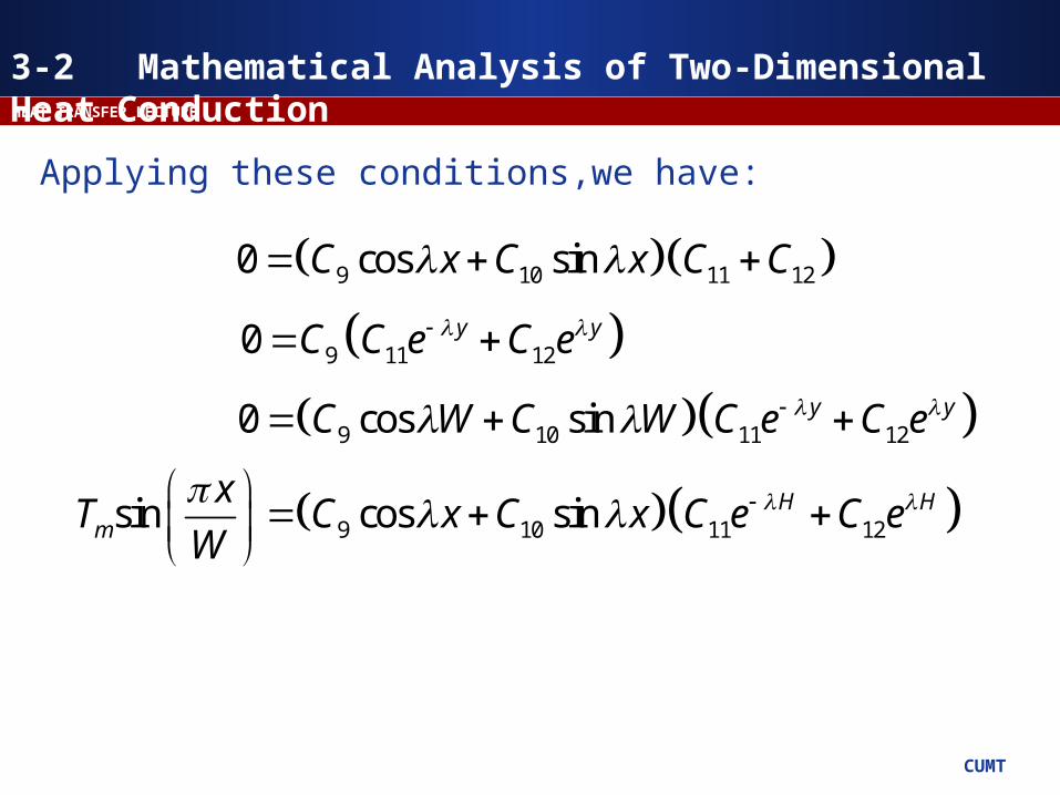
Applying these conditions,we have:
9 10 11 120 cos sinC x C x C C
9 11 120 y yC C e C e
9 10 11 120 cos sin y yC W C W C e C e
9 10 11 12sin cos sin H Hm
xT C x C x C e C e
W
3-2 Mathematical Analysis of Two-Dimensional Heat Conduction

CUMT
HEAT TRANSFER LECTURE
accordingly,
and from (c),
This requires that
11 12C C
9 0C
10 120 sin y yC C W e e
sin 0W
3-2 Mathematical Analysis of Two-Dimensional Heat Conduction
CUMT
HEAT TRANSFER LECTURE
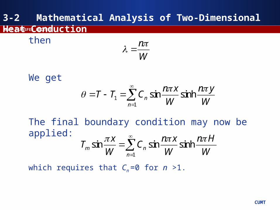
then
which requires that Cn =0 for n >1.
We get
n
W
11
sin sinhnn
n x n yT T C
W W
1
sin sin sinhm nn
x n x n HT C
W W W
The final boundary condition may now be applied:
3-2 Mathematical Analysis of Two-Dimensional Heat Conduction

CUMT
HEAT TRANSFER LECTURE
The final solution is therefore
1
sinh /sin
sinh /m
y W xT T T
H W W
The temperature field for this problem is shown. Note that the heat-flow lines are perpendicular to the isotherms.
3-2 Mathematical Analysis of Two-Dimensional Heat Conduction
CUMT
HEAT TRANSFER LECTURE
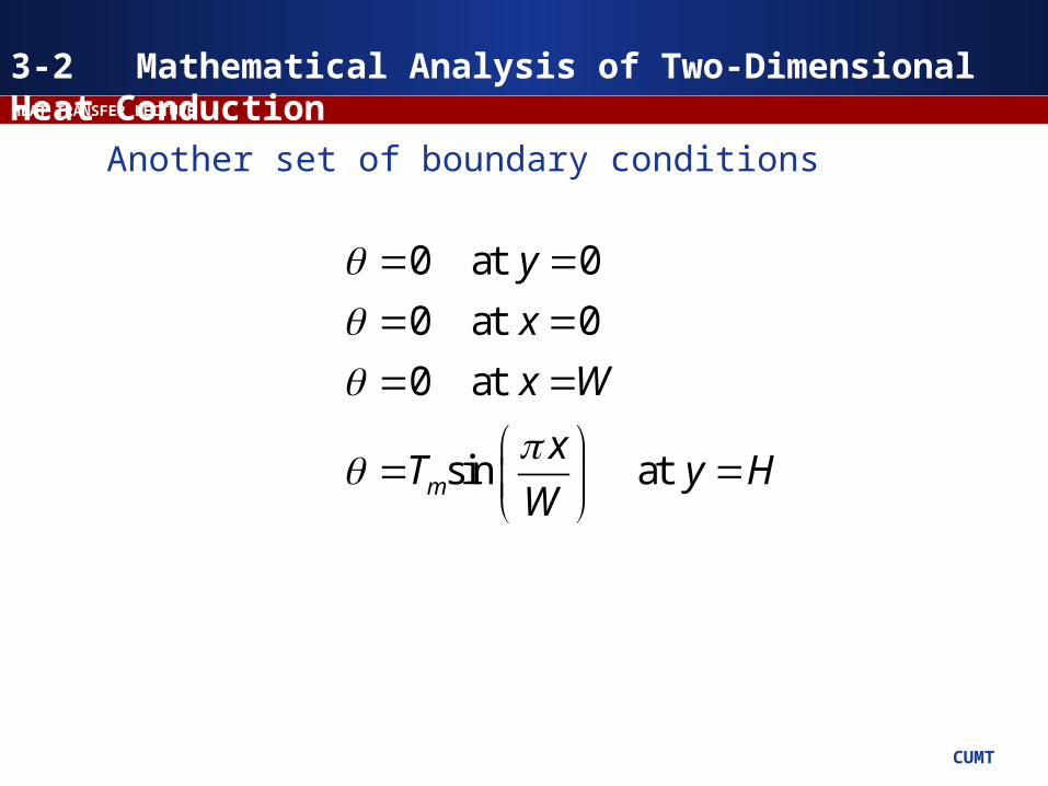
Another set of boundary conditions
0 at 0
0 at 0
0 at
sin at m
y
x
x W
xT y H
W
3-2 Mathematical Analysis of Two-Dimensional Heat Conduction
CUMT
HEAT TRANSFER LECTURE
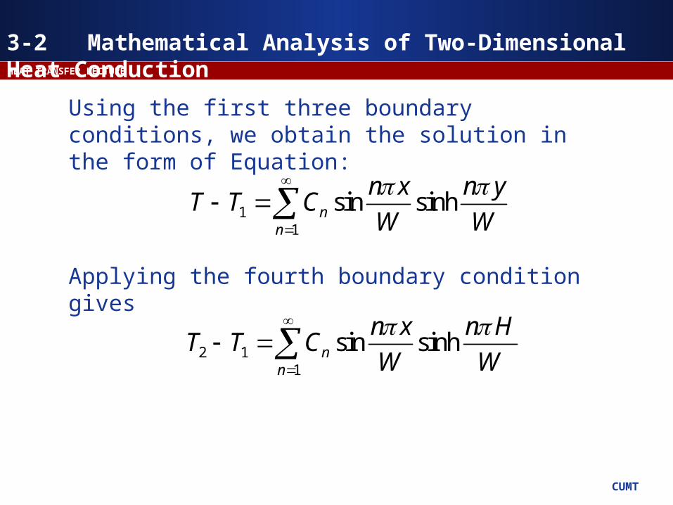
Using the first three boundary conditions, we obtain the solution in the form of Equation:
11
sin sinhnn
n x n yT T C
W W
Applying the fourth boundary condition gives
2 11
sin sinhnn
n x n HT T C
W W
3-2 Mathematical Analysis of Two-Dimensional Heat Conduction
CUMT
HEAT TRANSFER LECTURE
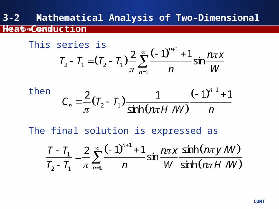
This series is
then
1
2 1 2 11
1 12sin
n
n
n xT T T T
n W
1
2 1
1 12 1
sinh /
n
nC T Tn H W n
The final solution is expressed as
1
1
12 1
1 1 sinh /2sin
sinh /
n
n
n y WT T n x
T T n W n H W
3-2 Mathematical Analysis of Two-Dimensional Heat Conduction
CUMT
HEAT TRANSFER LECTURE
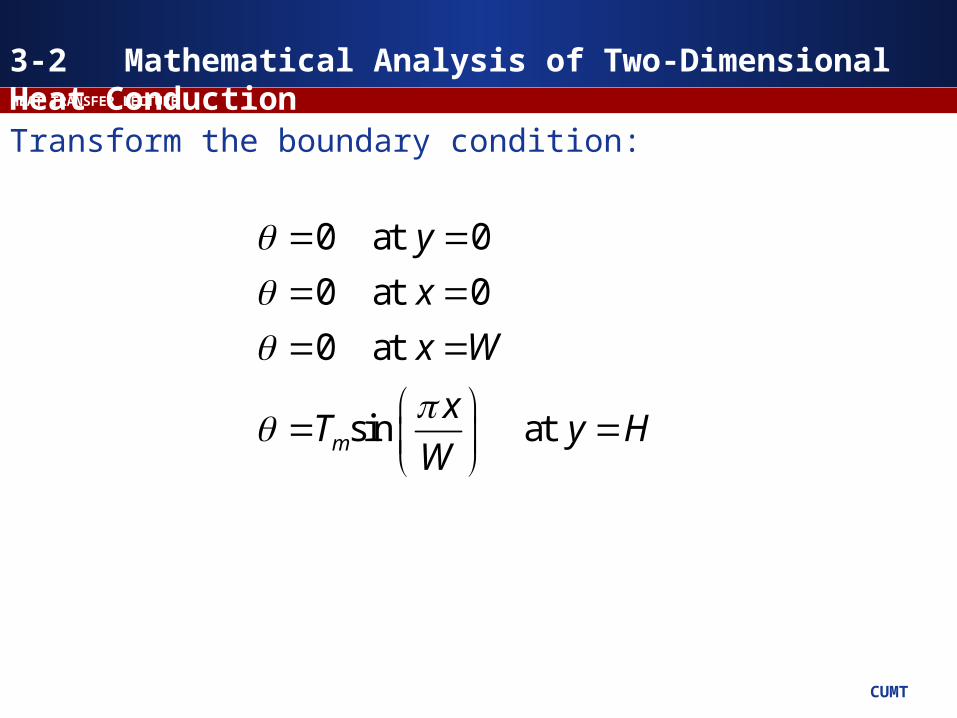
0 at 0
0 at 0
0 at
sin at m
y
x
x W
xT y H
W
Transform the boundary condition:
3-2 Mathematical Analysis of Two-Dimensional Heat Conduction

CUMT
HEAT TRANSFER LECTURE
3-3 Graphical Analysis
neglect
CUMT
HEAT TRANSFER LECTURE
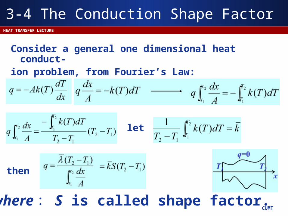
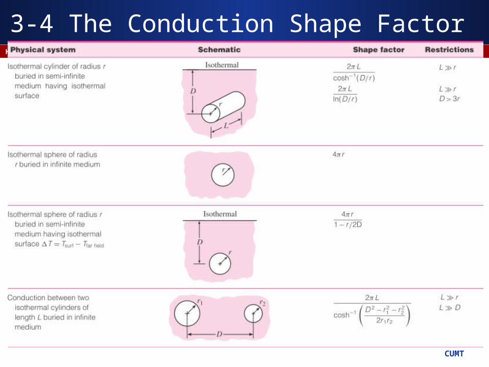
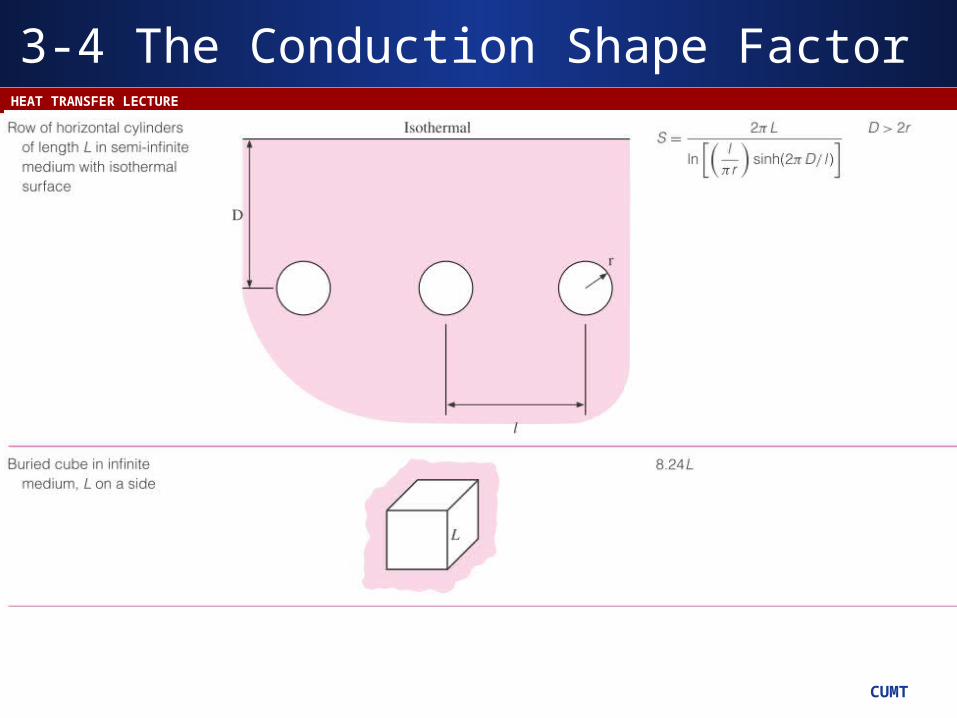
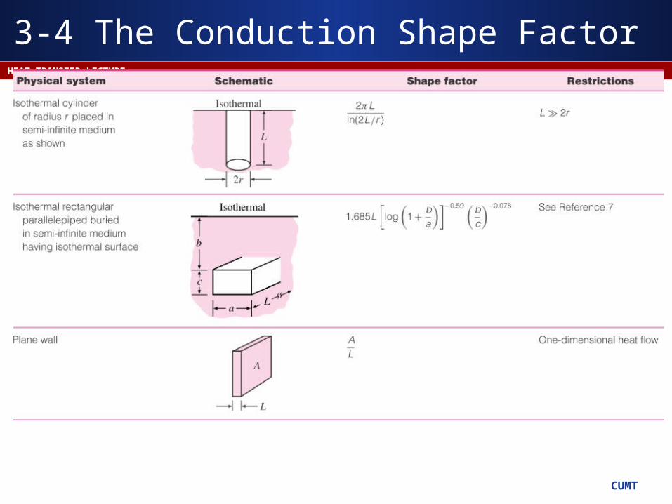
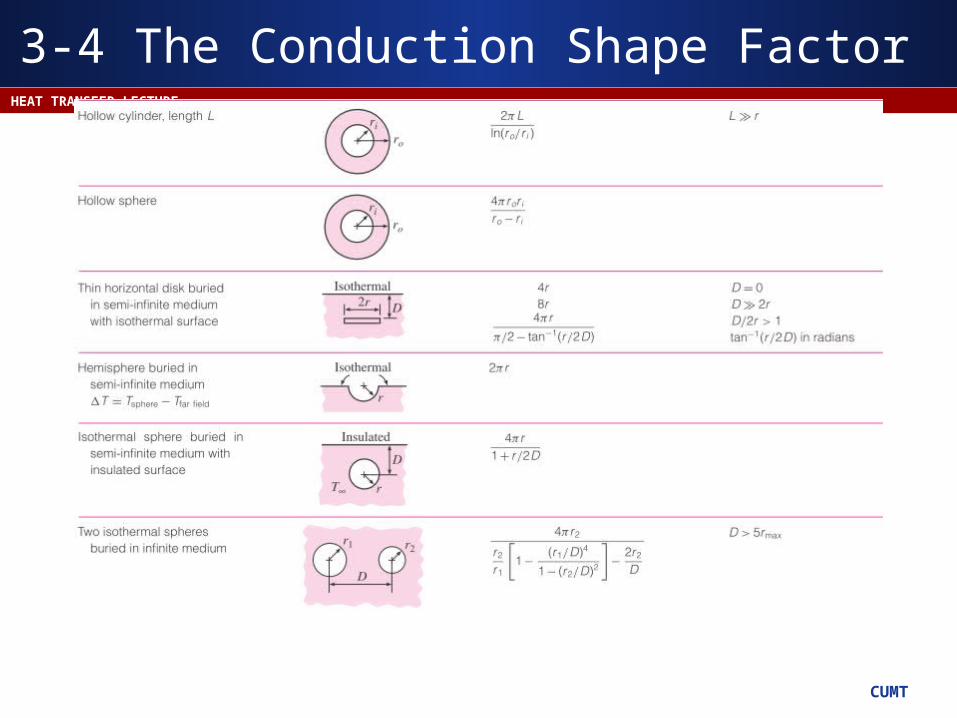
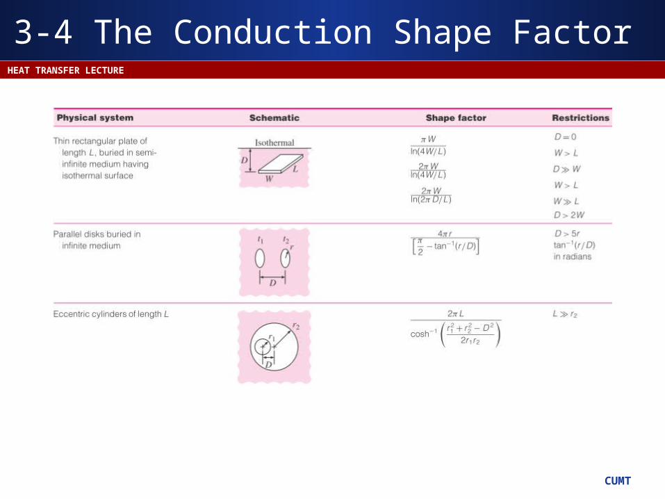
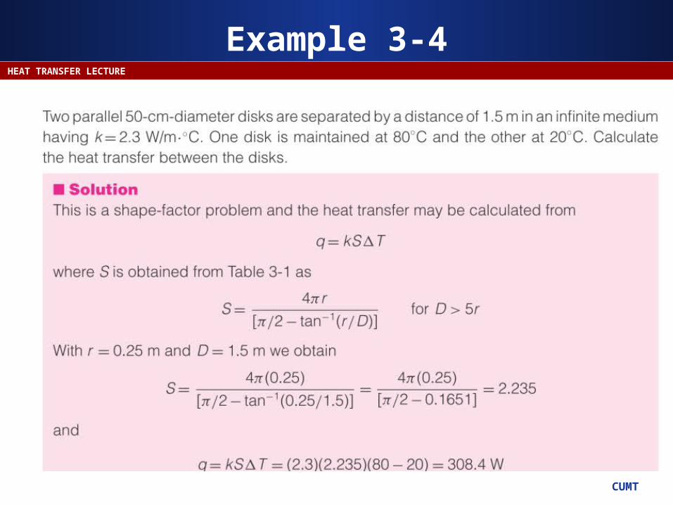
3-4 The Conduction Shape Factor
Consider a general one dimensional heat conduct-ion problem, from Fourier’s Law:
let
then
where: S is called shape factor.
CUMT
HEAT TRANSFER LECTURE
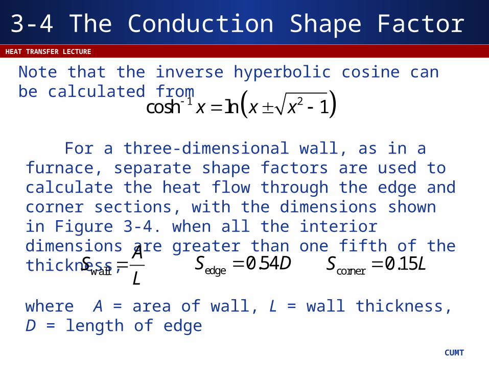
Note that the inverse hyperbolic cosine can be calculated from
1 2cosh ln 1x x x
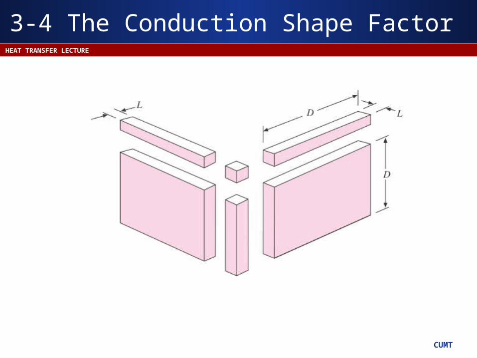
For a three-dimensional wall, as in a furnace, separate shape factors are used to calculate the heat flow through the edge and corner sections, with the dimensions shown in Figure 3-4. when all the interior dimensions are greater than one fifth of the thickness,
wall
AS
L edge 0.54S D corner 0.15S L
where A = area of wall, L = wall thickness, D = length of edge
3-4 The Conduction Shape Factor
CUMT
HEAT TRANSFER LECTURE
3-4 The Conduction Shape Factor
CUMT
HEAT TRANSFER LECTURE
3-4 The Conduction Shape Factor
CUMT
HEAT TRANSFER LECTURE
3-4 The Conduction Shape Factor
CUMT
HEAT TRANSFER LECTURE
3-4 The Conduction Shape Factor
CUMT
HEAT TRANSFER LECTURE
3-4 The Conduction Shape Factor
CUMT
HEAT TRANSFER LECTURE
3-4 The Conduction Shape Factor

CUMT
HEAT TRANSFER LECTURE
3-4 The Conduction Shape Factor
CUMT
HEAT TRANSFER LECTURE
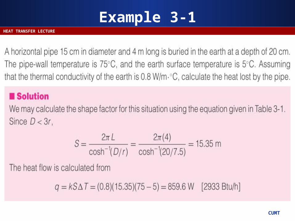
Example 3-1
CUMT
HEAT TRANSFER LECTURE
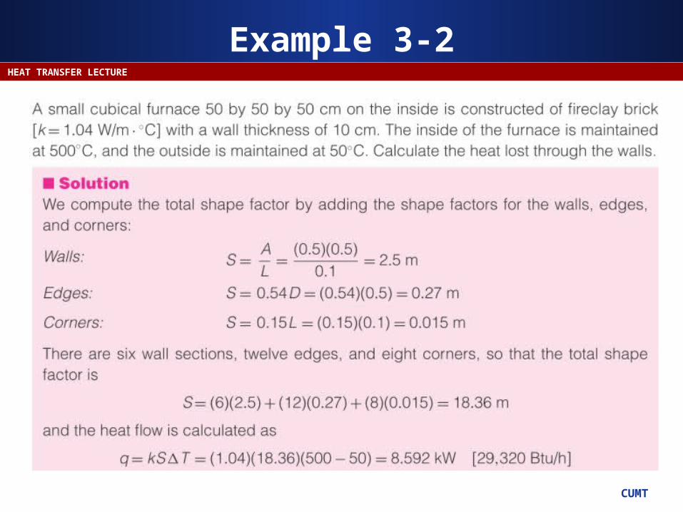
Example 3-2
CUMT
HEAT TRANSFER LECTURE
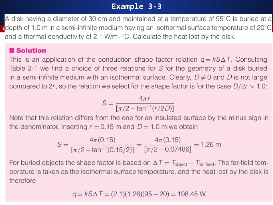
Example 3-3
CUMT
HEAT TRANSFER LECTURE
Example 3-4
CUMT
HEAT TRANSFER LECTURE
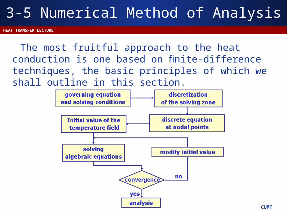
3-5 Numerical Method of Analysis
The most fruitful approach to the heat conduction is one based on finite-difference techniques, the basic principles of which we shall outline in this section.
CUMT
HEAT TRANSFER LECTURE
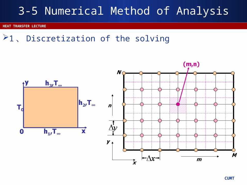
1 、 Discretization of the solving
3-5 Numerical Method of Analysis
CUMT
HEAT TRANSFER LECTURE
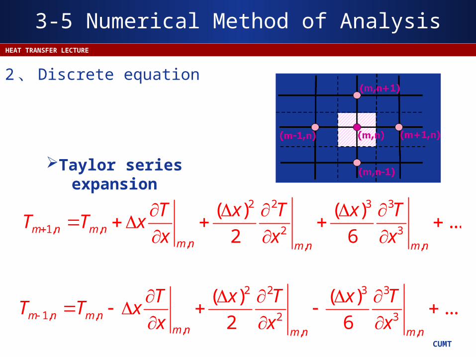
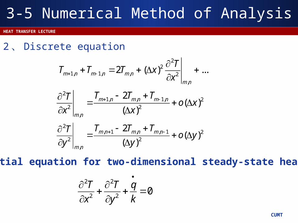
2 、 Discrete equation
Taylor series expansion
2 2 3 3
1, , 2 3, , ,
( ) ( )...
2 6m n m nm n m n m n
T x T x TT T x
x x x
2 2 3 3
1, , 2 3, , ,
( ) ( )...
2 6m n m nm n m n m n
T x T x TT T x
x x x
3-5 Numerical Method of Analysis
CUMT
HEAT TRANSFER LECTURE
22
1, 1, , 2
,
2 ( ) ...m n m n m n
m n
TT T T x
x
21, , 1, 2
2 2
,
2( )
( )m n m n m n
m n
T T TTo x
x x
22
1,,1,
,
2
2
)()(
2yo
y
TTT
y
T nmnmnm
nm
2 、 Discrete equation
Differential equation for two-dimensional steady-state heat flow
2 2
2 20
T T q
x y k
3-5 Numerical Method of Analysis
CUMT
HEAT TRANSFER LECTURE
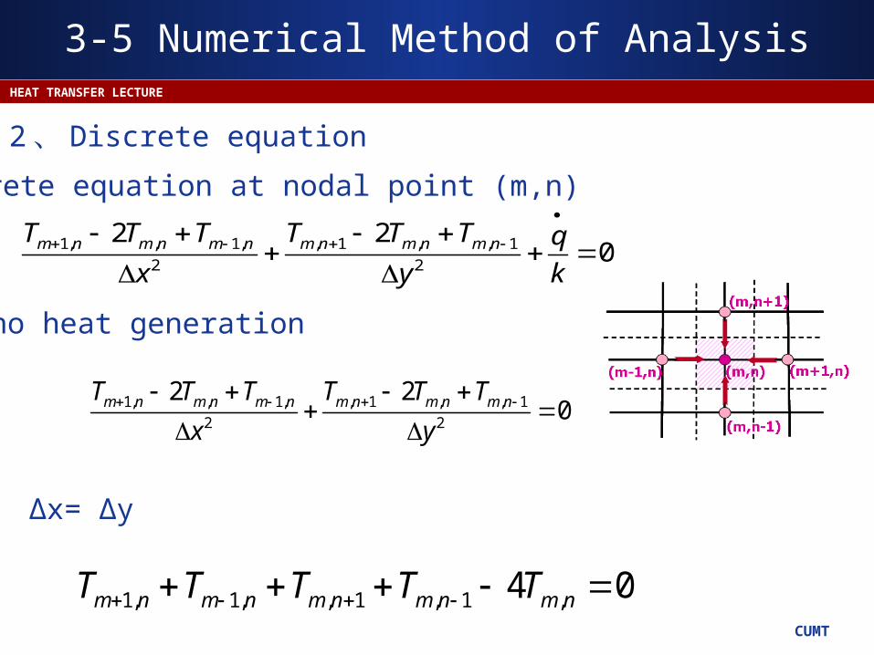
2 、 Discrete equation
Discrete equation at nodal point (m,n)
1, , 1, , 1 , , 1
2 2
2 20m n m n m n m n m n m nT T T T T T q
x y k
1, , 1, , 1 , , 1
2 2
2 20m n m n m n m n m n m nT T T T T T
x y
no heat generation
Δx= Δy
1, 1, , 1 , 1 ,4 0m n m n m n m n m nT T T T T
3-5 Numerical Method of Analysis
CUMT
HEAT TRANSFER LECTURE
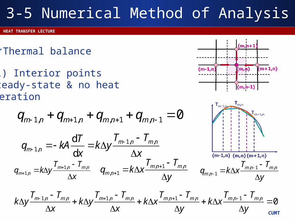
2 、 Discrete equationThermal balance
(1) Interior pointssteady-state & no heat
generation
1, 1, , 1 , 1 0m n m n m n m nq q q q
1, ,1,
d
dm n m n
m n
T TTq kA k y
x x
x
TTykq nmnm
nm
,,1,1
, 1 ,, 1
m n m nm n
T Tq k x
y
, 1 ,
, 1m n m n
m n
T Tq k x
y
1, , 1, , , 1 , , 1 , 0m n m n m n m n m n m n m n m nT T T T T T T Tk y k y k x k x
x x y y
3-5 Numerical Method of Analysis
CUMT
HEAT TRANSFER LECTURE
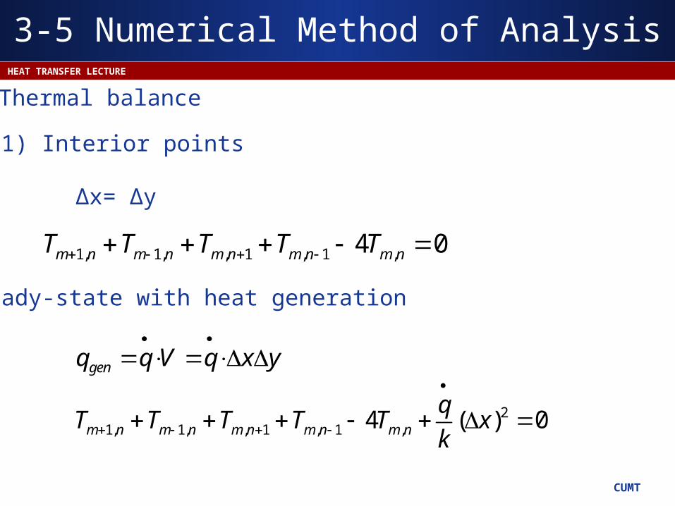
Thermal balance
Δx= Δy
1, 1, , 1 , 1 ,4 0m n m n m n m n m nT T T T T
genq q V q x y
21, 1, , 1 , 1 ,4 ( ) 0m n m n m n m n m n
qT T T T T x
k
steady-state with heat generation
(1) Interior points
3-5 Numerical Method of Analysis
CUMT
HEAT TRANSFER LECTURE
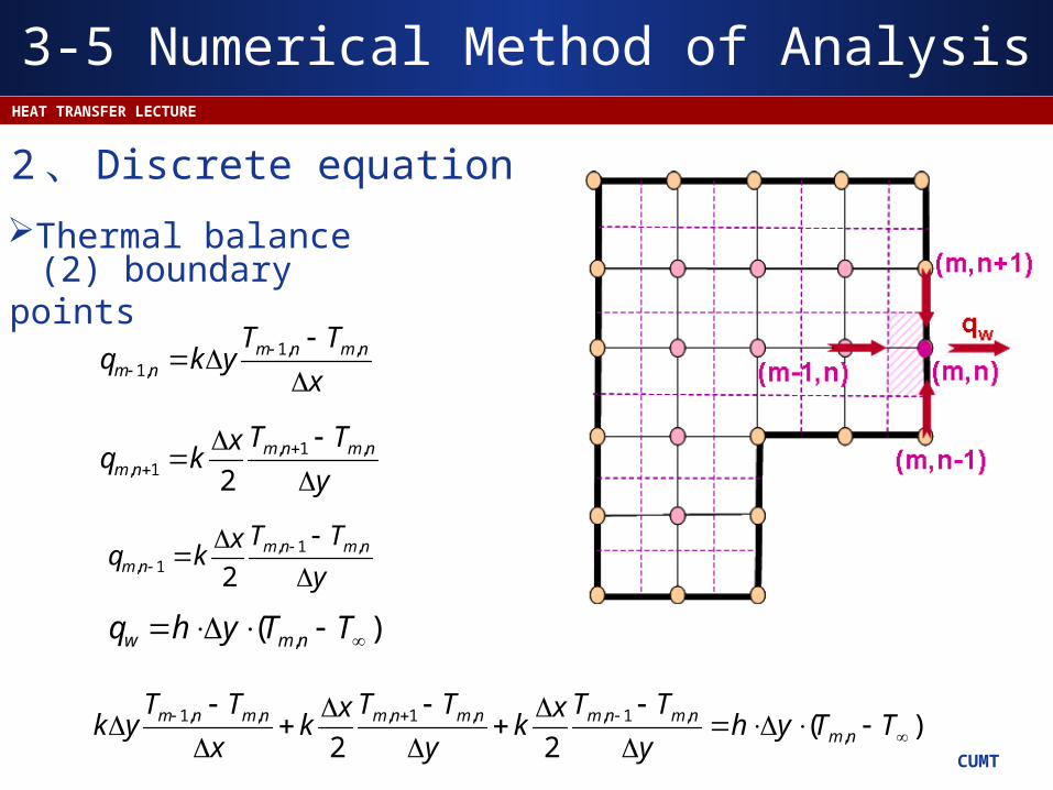
2 、 Discrete equation
Thermal balance(2) boundary
points1, ,
1,m n m n
m n
T Tq k y
x
, 1 ,, 1 2
m n m nm n
T Txq k
y
, 1 ,, 1 2
m n m nm n
T Txq k
y
,( )w m nq h y T T
1, , , 1 , , 1 ,,( )
2 2m n m n m n m n m n m n
m n
T T T T T Tx xk y k k h y T T
x y y
3-5 Numerical Method of Analysis
CUMT
HEAT TRANSFER LECTURE
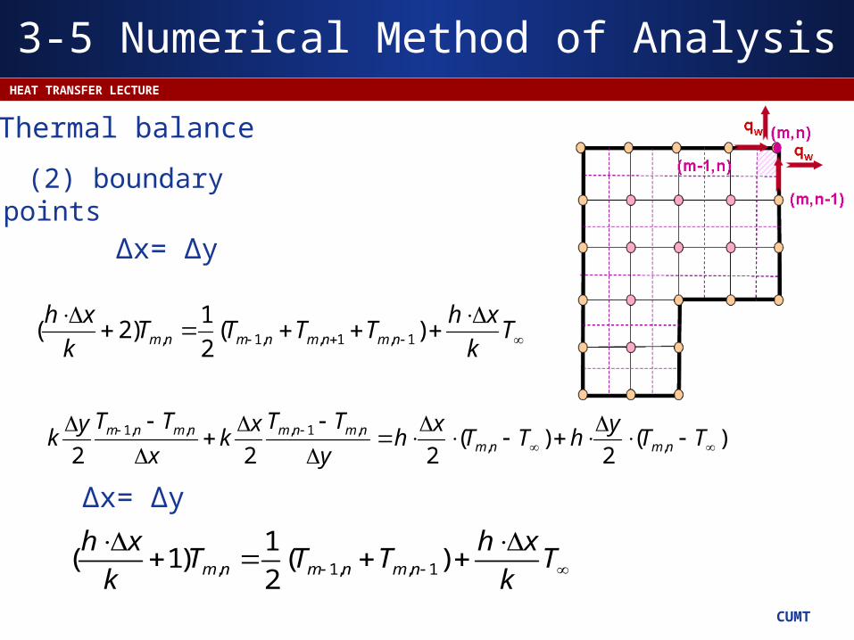
Thermal balance
Δx= Δy
(2) boundary points
, 1, , 1 , 1
1( 2) ( )
2m n m n m n m n
h x h xT T T T T
k k
1, , , 1 ,, ,( ) ( )
2 2 2 2m n m n m n m n
m n m n
T T T Ty x x yk k h T T h T T
x y
, 1, , 1
1( 1) ( )
2m n m n m n
h x h xT T T T
k k
Δx= Δy
3-5 Numerical Method of Analysis
CUMT
HEAT TRANSFER LECTURE
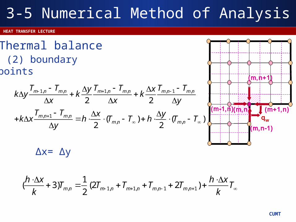
Thermal balance(2) boundary
points
Δx= Δy
1, , 1, , , 1 ,
, 1 ,, ,
2 2
( ) ( )2 2
m n m n m n m n m n m n
m n m nm n m n
T T T T T Ty xk y k k
x x y
T T x yk x h T T h T T
y
, 1, 1, , 1 , 1
1( 3) (2 2 )
2m n m n m n m n m n
h x h xT T T T T T
k k
3-5 Numerical Method of Analysis
CUMT
HEAT TRANSFER LECTURE
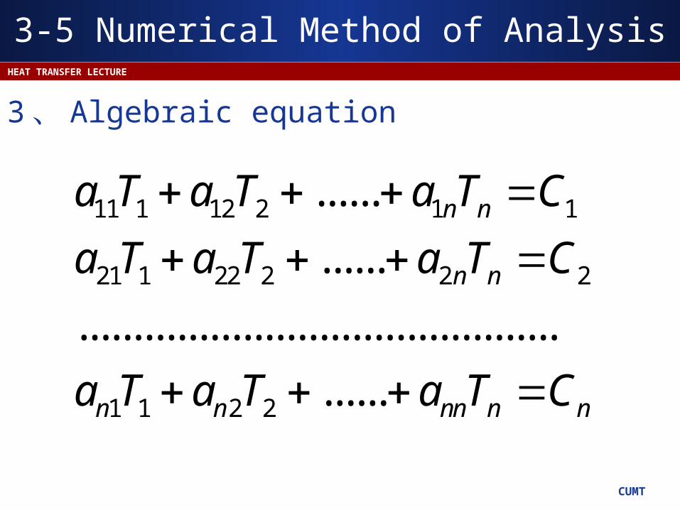
3 、 Algebraic equation
11 1 12 2 1 1
21 1 22 2 2 2
1 1 2 2
......
......
............................................
......
n n
n n
n n nn n n
a T a T a T C
a T a T a T C
a T a T a T C
3-5 Numerical Method of Analysis
CUMT
HEAT TRANSFER LECTURE
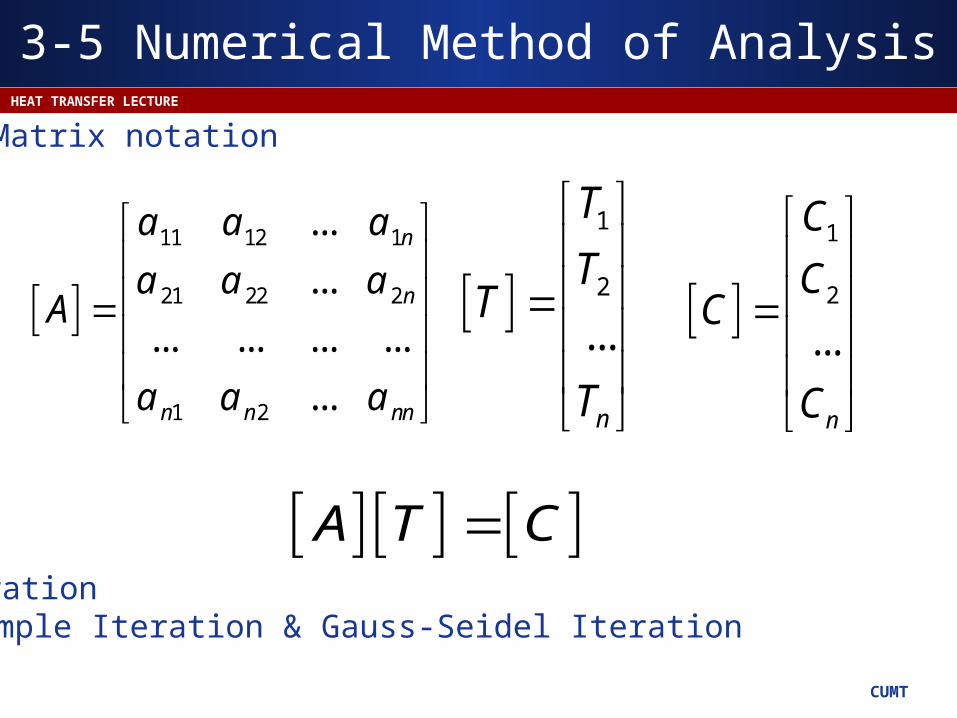
Matrix notation
11 12 1
21 22 2
1 2
...
...
... ... ... ...
...
n
n
n n nn
a a a
a a aA
a a a
1
2
...
n
T
TT
T
1
2
...
n
C
CC
C
A T CIteration Simple Iteration & Gauss-Seidel Iteration
3-5 Numerical Method of Analysis
CUMT
HEAT TRANSFER LECTURE
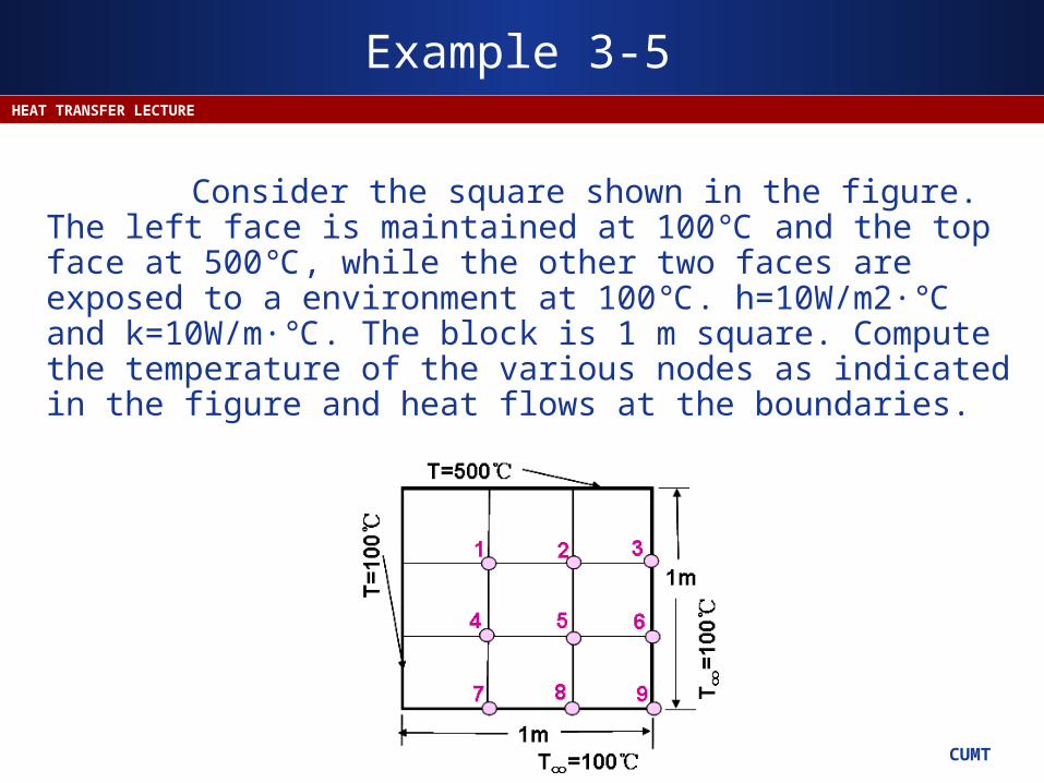
Example 3-5
Consider the square shown in the figure. The left face is maintained at 100 and the top face at 500 , while the ℃ ℃other two faces are exposed to a environment at 100 . ℃h=10W/m2· and k=10W/m· . The block is 1 m ℃ ℃square. Compute the temperature of the various nodes as indicated in the figure and heat flows at the boundaries.
CUMT
HEAT TRANSFER LECTURE
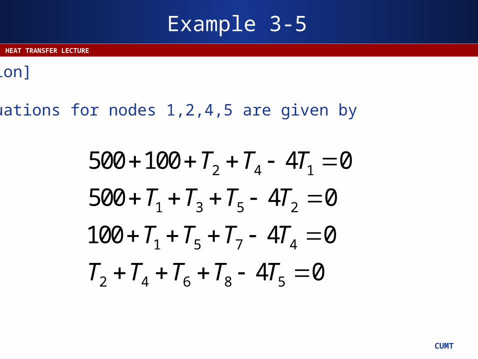
[Solution]
The equations for nodes 1,2,4,5 are given by
2 4 1
1 3 5 2
1 5 7 4
2 4 6 8 5
500 100 4 0
500 4 0
100 4 0
4 0
T T T
T T T T
T T T T
T T T T T
Example 3-5
CUMT
HEAT TRANSFER LECTURE
[Solution]
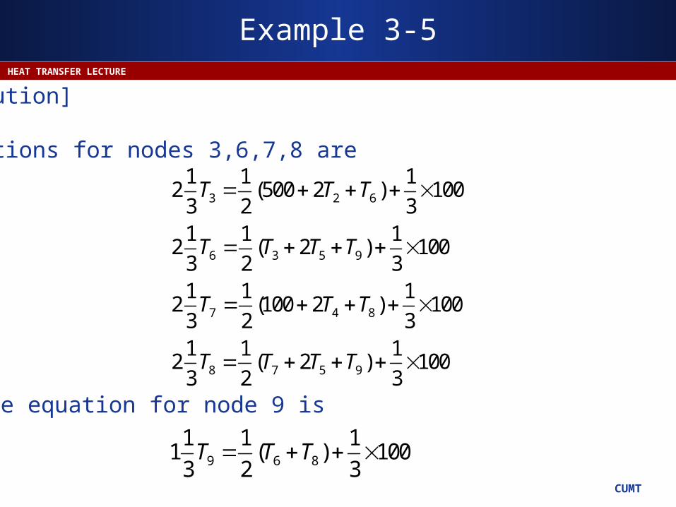
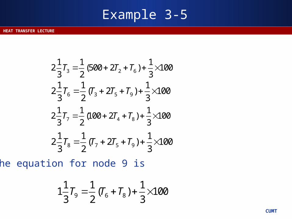
Equations for nodes 3,6,7,8 are
The equation for node 9 is
9 6 8
1 1 11 ( ) 100
3 2 3T T T
3 2 6
6 3 5 9
7 4 8
8 7 5 9
1 1 12 (500 2 ) 100
3 2 31 1 1
2 ( 2 ) 1003 2 31 1 1
2 (100 2 ) 1003 2 31 1 1
2 ( 2 ) 1003 2 3
T T T
T T T T
T T T
T T T T
Example 3-5
CUMT
HEAT TRANSFER LECTURE
3 2 6
1 1 12 (500 2 ) 100
3 2 3T T T
6 3 5 9
1 1 12 ( 2 ) 100
3 2 3T T T T
7 4 8
1 1 12 (100 2 ) 100
3 2 3T T T
8 7 5 9
1 1 12 ( 2 ) 100
3 2 3T T T T
The equation for node 9 is
9 6 8
1 1 11 ( ) 100
3 2 3T T T
Example 3-5
CUMT
HEAT TRANSFER LECTURE
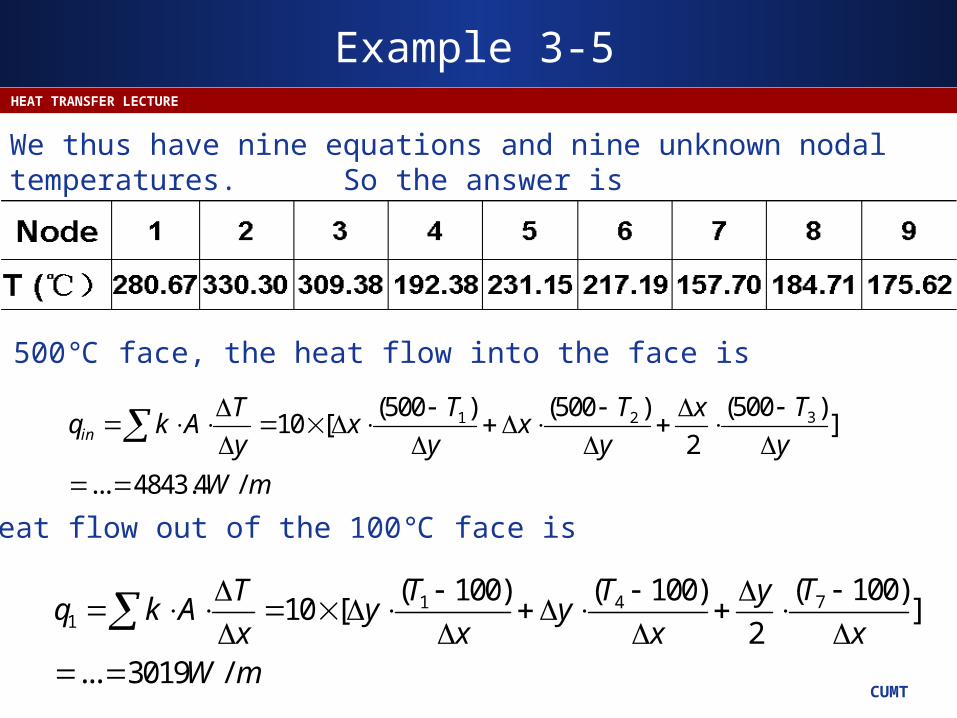
We thus have nine equations and nine unknown nodal temperatures. So the answer is
For the 500 face, the heat flow into the face is℃
31 2 (500 )(500 ) (500 )10 [ ]
2
... 4843.4 /
in
TT TT xq k A x x
y y y y
W m
The heat flow out of the 100 face is℃
71 41
( 100)( 100) ( 100)10 [ ]
2... 3019 /
TT TT yq k A y y
x x x xW m
Example 3-5
CUMT
HEAT TRANSFER LECTURE
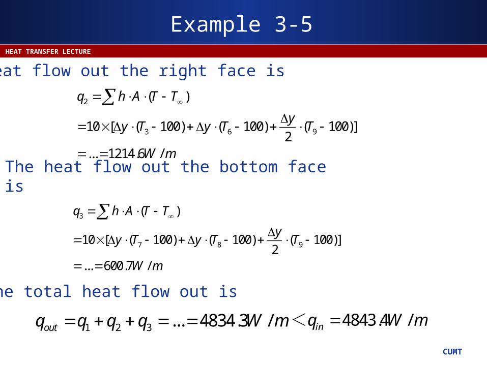
2
3 6 9
( )
10 [ ( 100) ( 100) ( 100)]2
... 1214.6 /
q h A T T
yy T y T T
W m
The heat flow out the right face is
3
7 8 9
( )
10 [ ( 100) ( 100) ( 100)]2
... 600.7 /
q h A T T
yy T y T T
W m
1 2 3 ... 4834.3 /outq q q q W m 4843.4 /inq W m<
The heat flow out the bottom face is
The total heat flow out is
Example 3-5
CUMT
HEAT TRANSFER LECTURE
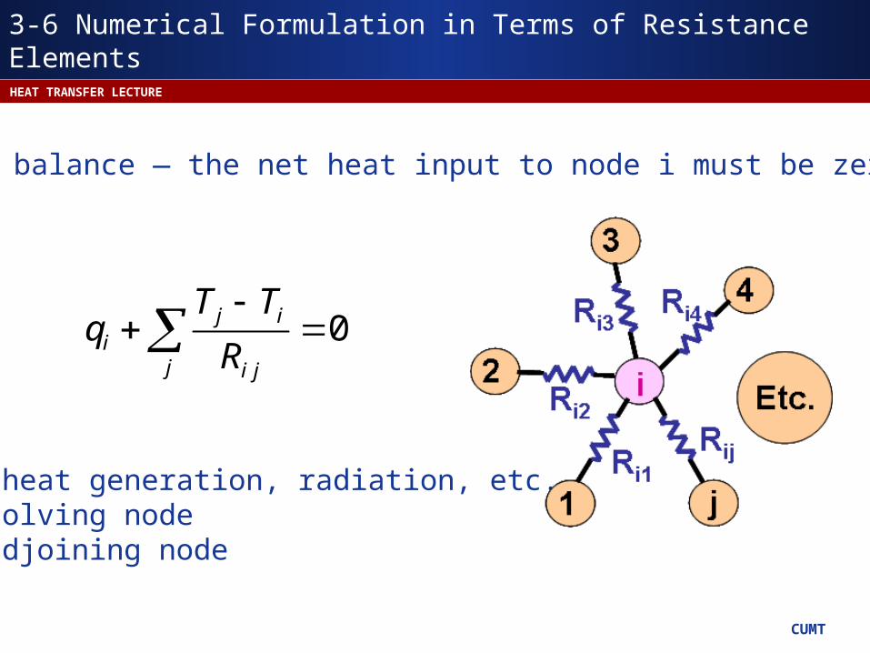
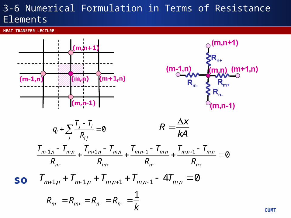
3-6 Numerical Formulation in Terms of Resistance Elements
Thermal balance — the net heat input to node i must be zero
0j ii
j i j
T Tq
R
qi — heat generation, radiation, etc.i — solving nodej — adjoining node
CUMT
HEAT TRANSFER LECTURE
1, , 1, , , 1 , , 1 , 0m n m n m n m n m n m n m n m n
m m n n
T T T T T T T T
R R R R
xR
kA
1m m n nR R R R
k
1, 1, , 1 , 1 ,4 0m n m n m n m n m nT T T T T
0j ii
j i j
T Tq
R
so
3-6 Numerical Formulation in Terms of Resistance Elements
CUMT
HEAT TRANSFER LECTURE
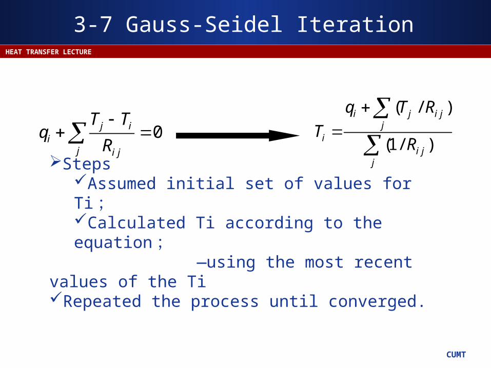
3-7 Gauss-Seidel Iteration
0j ii
j i j
T Tq
R
( / )
(1/ )
i j i jj
ii j
j
q T R
TR
StepsAssumed initial set of values for Ti;Calculated Ti according to the equation;
—using the most recent values of the TiRepeated the process until converged.
CUMT
HEAT TRANSFER LECTURE
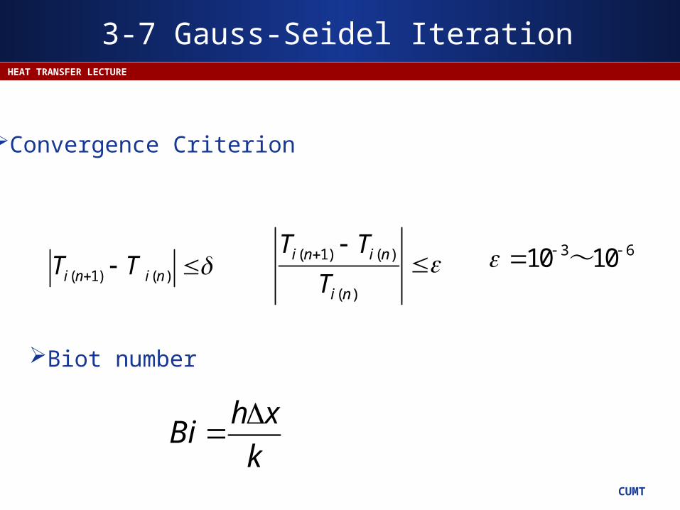
Convergence Criterion
( 1) ( )i n i nT T ( 1) ( )
( )
i n i n
i n
T T
T
3 610 10 ~
Biot number
h xBi
k
3-7 Gauss-Seidel Iteration
CUMT
HEAT TRANSFER LECTURE
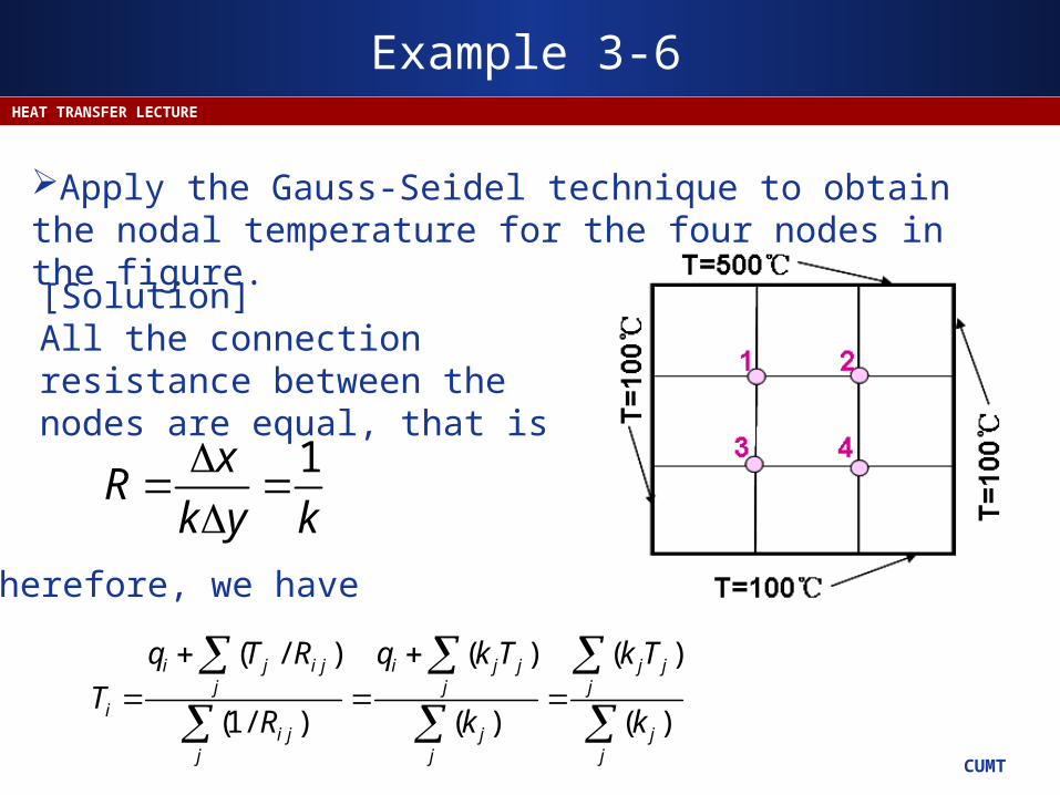
Example 3-6
1xR
k y k
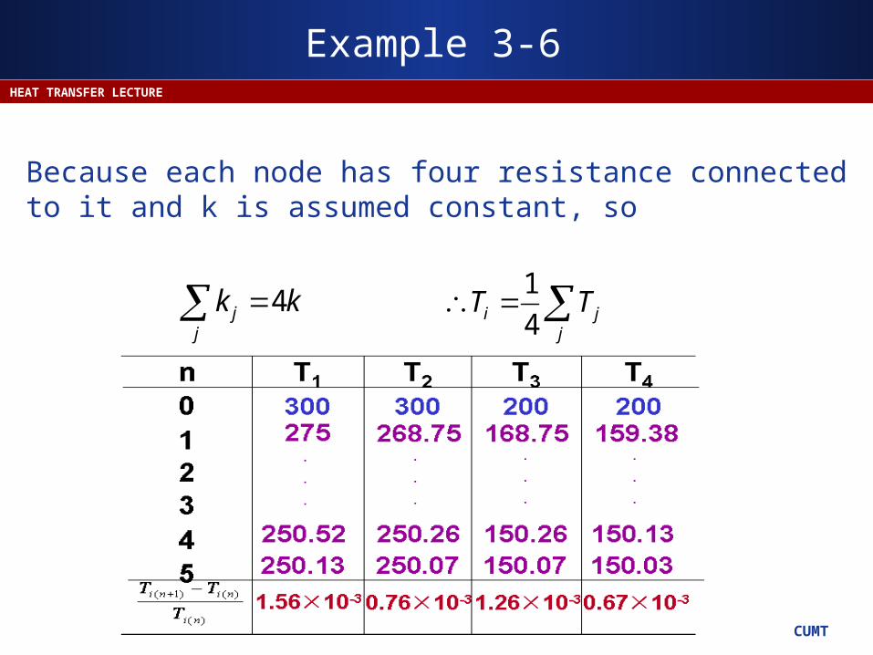
Apply the Gauss-Seidel technique to obtain the nodal temperature for the four nodes in the figure.
[Solution]All the connection resistance between the nodes are equal, that is
Therefore, we have
( / ) ( ) ( )
(1/ ) ( ) ( )
i j i j i j j j jj j j
ii j j j
j j j
q T R q k T k T
TR k k
CUMT
HEAT TRANSFER LECTURE
Example 3-6
Because each node has four resistance connected to it and k is assumed constant, so
4jj
k k 1
4i jj
T T
CUMT
HEAT TRANSFER LECTURE
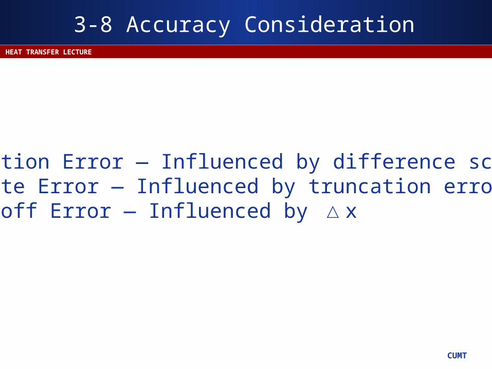
3-8 Accuracy Consideration
Truncation Error — Influenced by difference schemeDiscrete Error — Influenced by truncation error & x△Round-off Error — Influenced by x△
CUMT
HEAT TRANSFER LECTURE
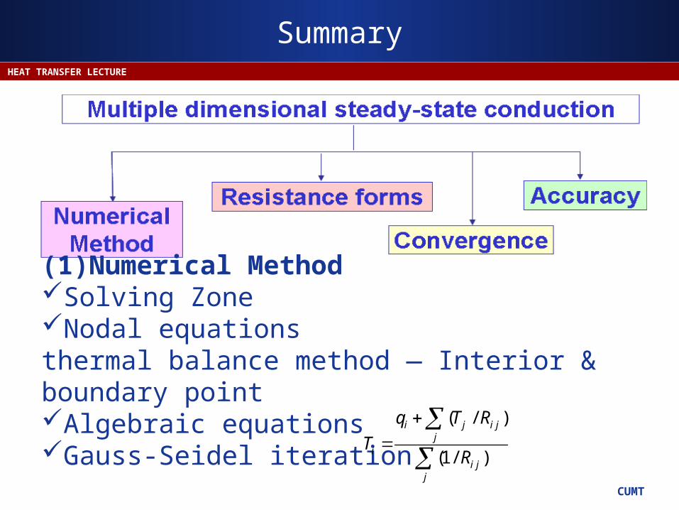
Summary
(1)Numerical MethodSolving ZoneNodal equationsthermal balance method — Interior & boundary pointAlgebraic equationsGauss-Seidel iteration
( / )
(1/ )
i j i jj
ii j
j
q T R
TR

CUMT
HEAT TRANSFER LECTURE
Summary
(2)Resistance Forms
0j ii
j i j
T Tq
R
(3)Convergence
Convergence Criterion
( 1) ( )i n i nT T
( 1) ( )i n i nT T
CUMT
HEAT TRANSFER LECTURE
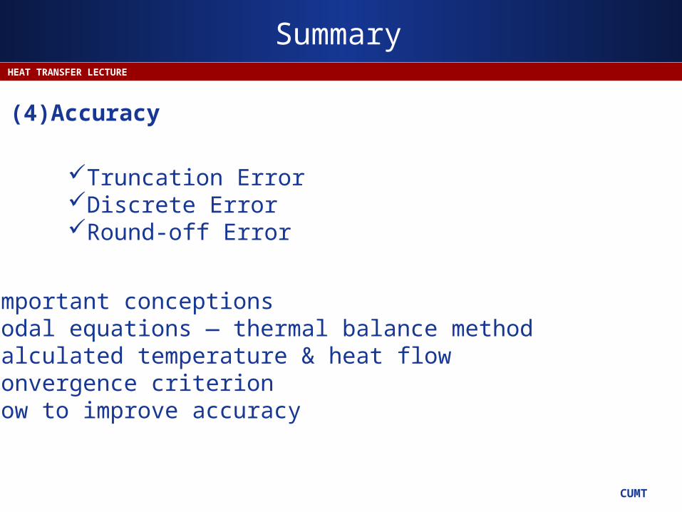
Summary
(4)Accuracy
Truncation ErrorDiscrete ErrorRound-off Error
Important conceptionsNodal equations — thermal balance methodCalculated temperature & heat flowConvergence criterionHow to improve accuracy
CUMT
HEAT TRANSFER LECTURE
Exercises
Exercises: 3-16, 3-24, 3-48, 3-59