CSc340 9b 1

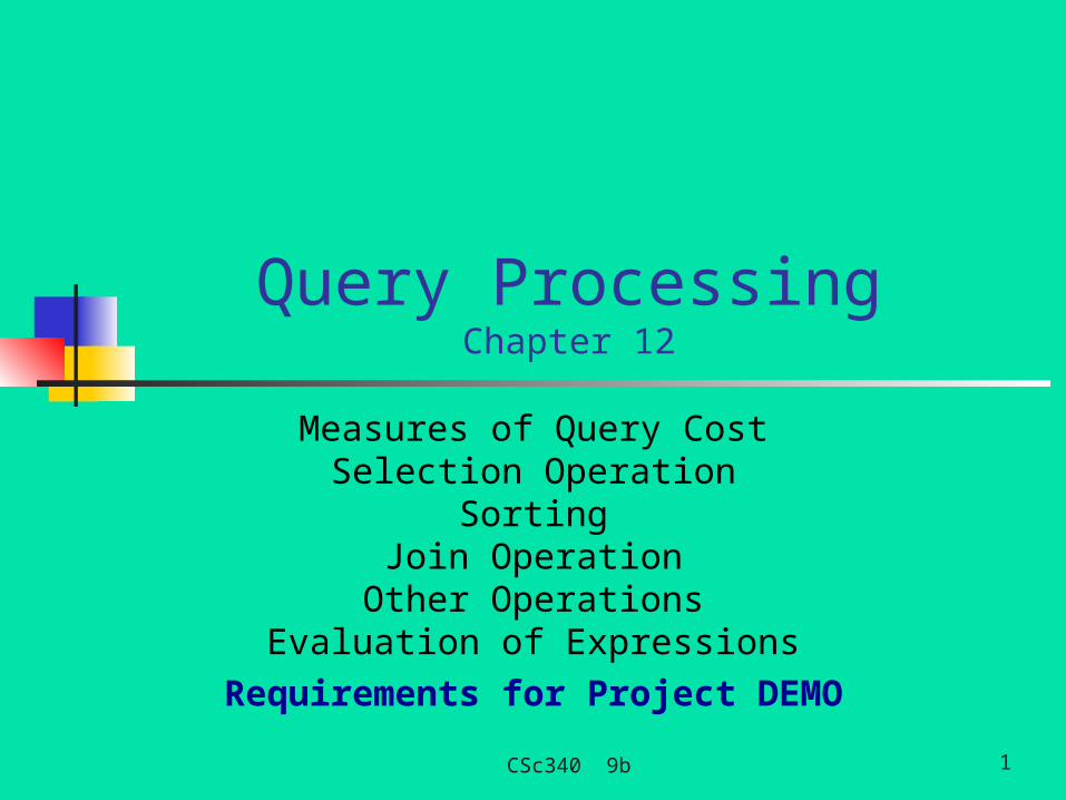
Query ProcessingChapter 12

Measures of Query CostSelection Operation

SortingJoin Operation

Other OperationsEvaluation of Expressions

Requirements for Project DEMO

CSc-340 9b 2

Collect Homework

Chapter 10

CS Seminar

12:50 in Olin 107

CSc340 9b 3

Basic Steps in Query Processing

1. Parsing and translation2. Optimization3. Evaluation

Basic Steps in Query Processing (Cont.)

Parsing and translation translate the query into its internal form. This is then

translated into relational algebra. Parser checks syntax, verifies relations

Evaluation The query-execution engine takes a query-evaluation

plan, executes that plan, and returns the answers to the query.

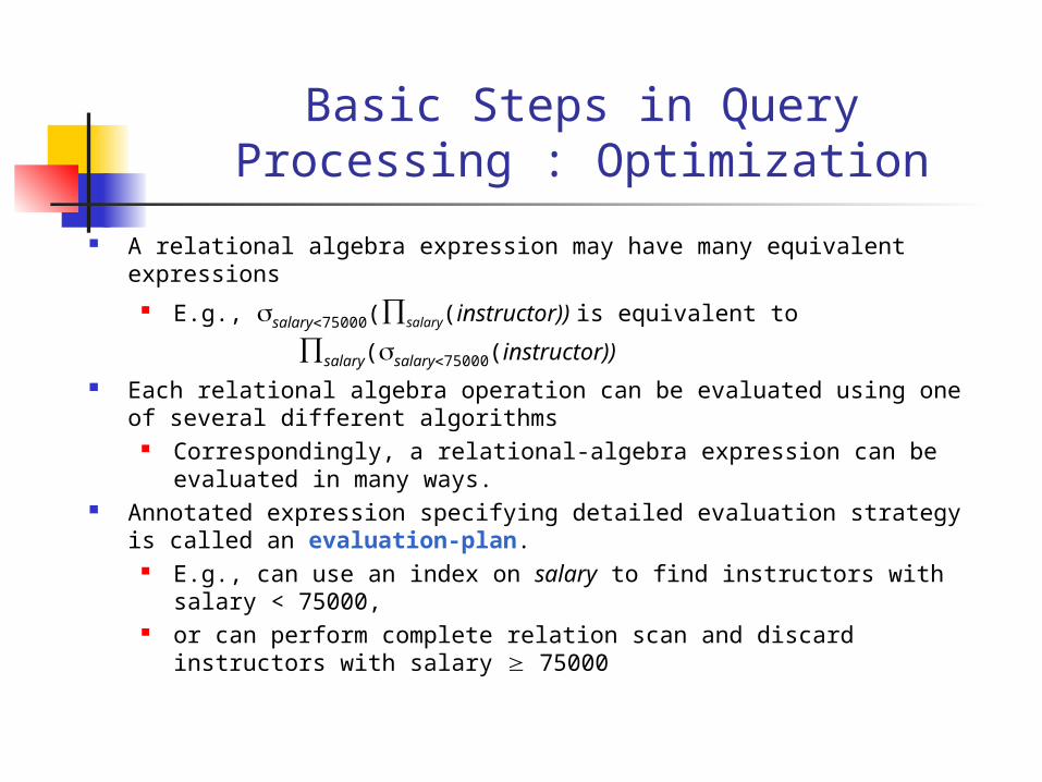
Basic Steps in Query Processing : Optimization

A relational algebra expression may have many equivalent expressions E.g., salary75000(salary(instructor)) is equivalent to

salary(salary75000(instructor)) Each relational algebra operation can be evaluated using one of several

different algorithms Correspondingly, a relational-algebra expression can be evaluated in

many ways. Annotated expression specifying detailed evaluation strategy is called an

evaluation-plan. E.g., can use an index on salary to find instructors with salary <

75000, or can perform complete relation scan and discard instructors with

salary 75000

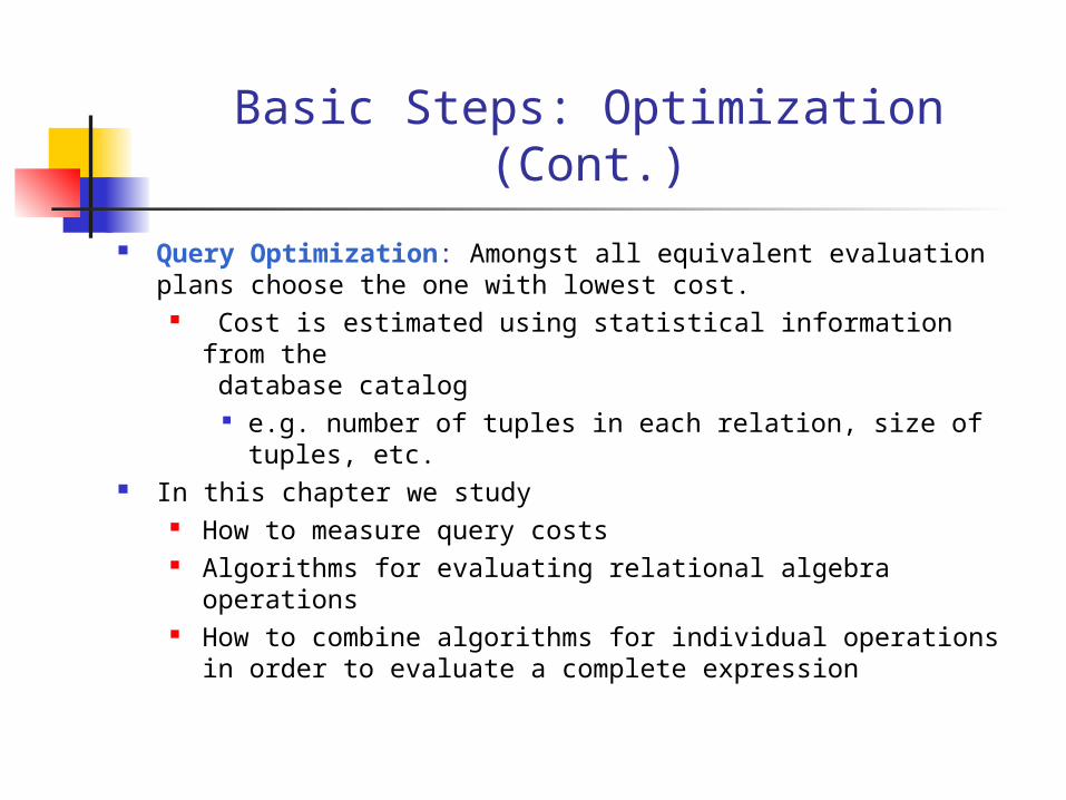
Basic Steps: Optimization (Cont.)

Query Optimization: Amongst all equivalent evaluation plans choose the one with lowest cost.

Cost is estimated using statistical information from the database catalog

e.g. number of tuples in each relation, size of tuples, etc.

In this chapter we study How to measure query costs Algorithms for evaluating relational algebra operations How to combine algorithms for individual operations in

order to evaluate a complete expression

Memory Hierarchy and the Speaker on Tuesday

CPU Scheduling: Cache Primary Memory

240 times slower

Indexing (ch 11) & SQL Processing (ch 12) Primary Memory vs. Disk Storage (Secondary Memory)

Thousands of times slower! Using Mag Tape for Secondary Memory

CSc340 9b 8

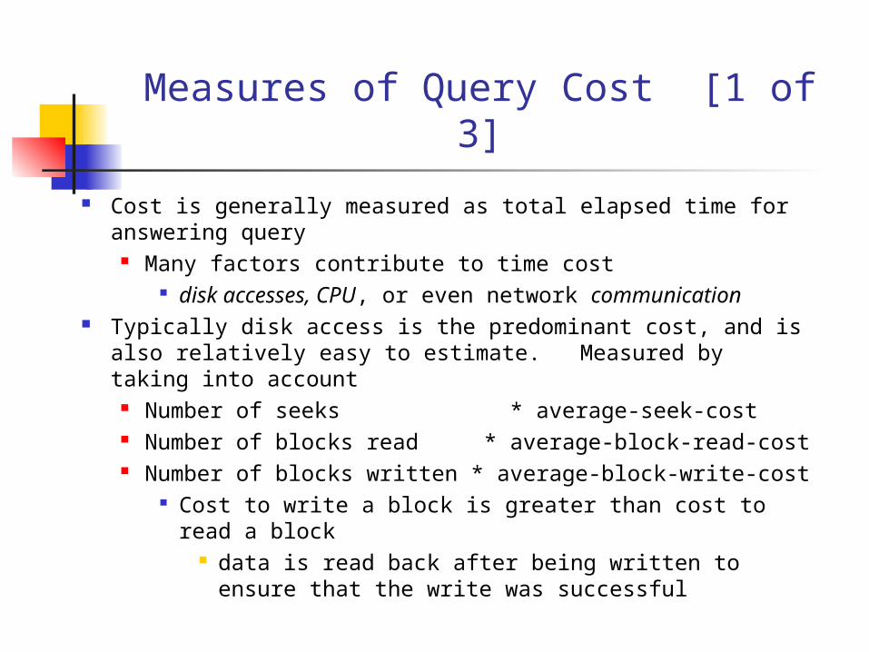
Measures of Query Cost [1 of 3]

Cost is generally measured as total elapsed time for answering query

Many factors contribute to time cost disk accesses, CPU, or even network communication

Typically disk access is the predominant cost, and is also relatively easy to estimate. Measured by taking into account

Number of seeks * average-seek-cost Number of blocks read * average-block-read-cost Number of blocks written * average-block-write-cost

Cost to write a block is greater than cost to read a block

data is read back after being written to ensure that the write was successful

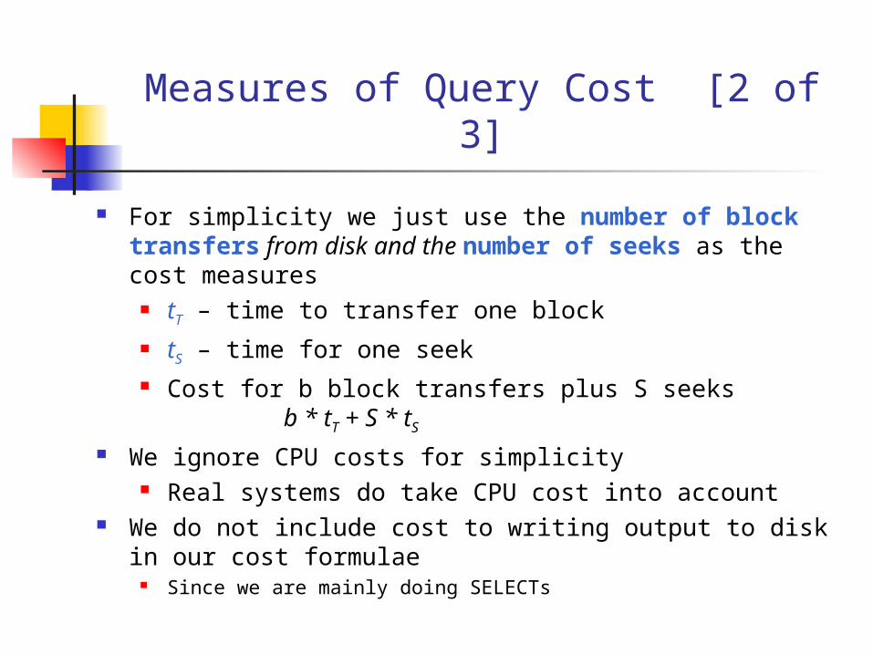
Measures of Query Cost [2 of 3]

For simplicity we just use the number of block transfers from disk and the number of seeks as the cost measures

tT – time to transfer one block tS – time for one seek Cost for b block transfers plus S seeks

b * tT + S * tS We ignore CPU costs for simplicity

Real systems do take CPU cost into account We do not include cost to writing output to disk in our cost

formulae Since we are mainly doing SELECTs

Measures of Query Cost [3 of 3]

Several algorithms can reduce disk IO by using extra buffer space

Amount of real memory available to buffer depends on other concurrent queries and OS processes, known only during execution

We often use worst case estimates, assuming only the minimum amount of memory needed for the operation is available

Required data may be buffer resident already, avoiding disk I/O

But hard to take into account for cost estimation

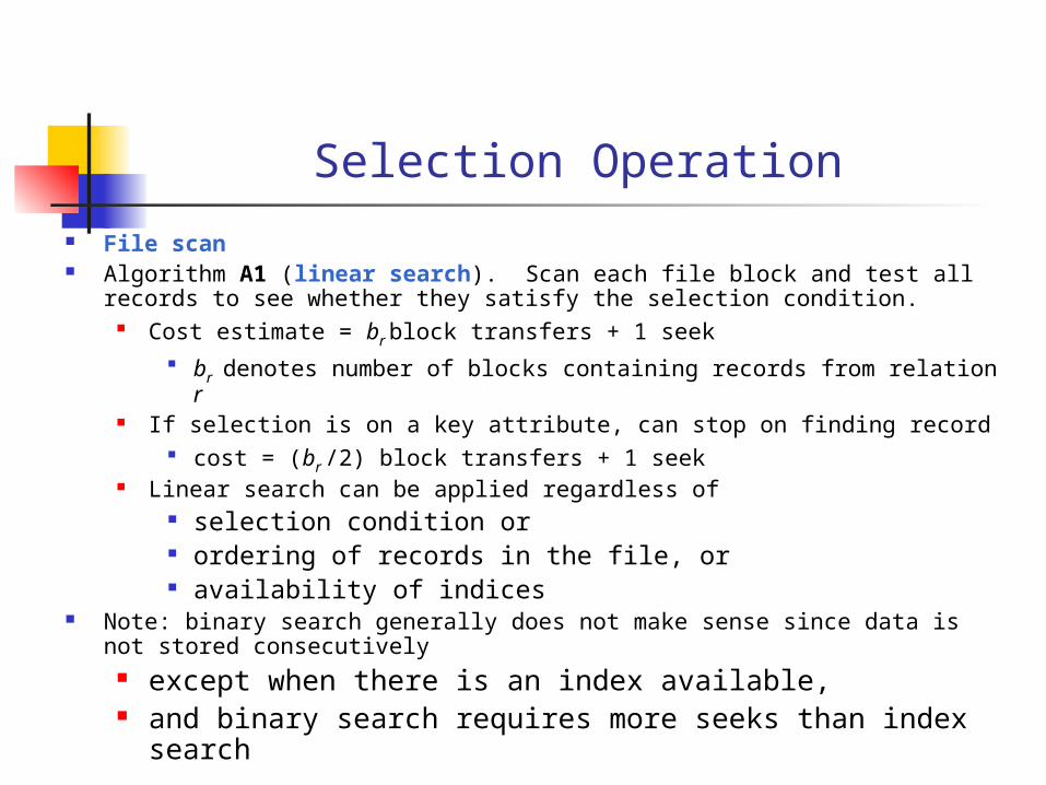
Selection Operation

File scan Algorithm A1 (linear search). Scan each file block and test all records to

see whether they satisfy the selection condition. Cost estimate = br block transfers + 1 seek

br denotes number of blocks containing records from relation r If selection is on a key attribute, can stop on finding record

cost = (br /2) block transfers + 1 seek Linear search can be applied regardless of

selection condition or ordering of records in the file, or availability of indices

Note: binary search generally does not make sense since data is not stored consecutively

except when there is an index available, and binary search requires more seeks than index search

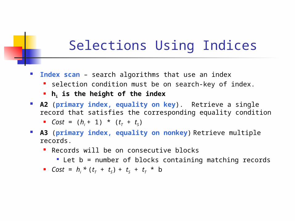
Selections Using Indices

Index scan – search algorithms that use an index selection condition must be on search-key of index. hi is the height of the index

A2 (primary index, equality on key). Retrieve a single record that satisfies the corresponding equality condition

Cost = (hi + 1) * (tT + tS) A3 (primary index, equality on nonkey) Retrieve multiple

records. Records will be on consecutive blocks

Let b = number of blocks containing matching records Cost = hi * (tT + tS) + tS + tT * b

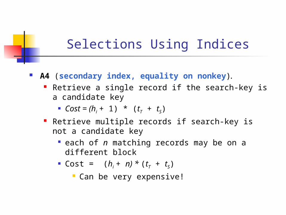
Selections Using Indices

A4 (secondary index, equality on nonkey). Retrieve a single record if the search-key is a

candidate key Cost = (hi + 1) * (tT + tS)

Retrieve multiple records if search-key is not a candidate key

each of n matching records may be on a different block

Cost = (hi + n) * (tT + tS) Can be very expensive!

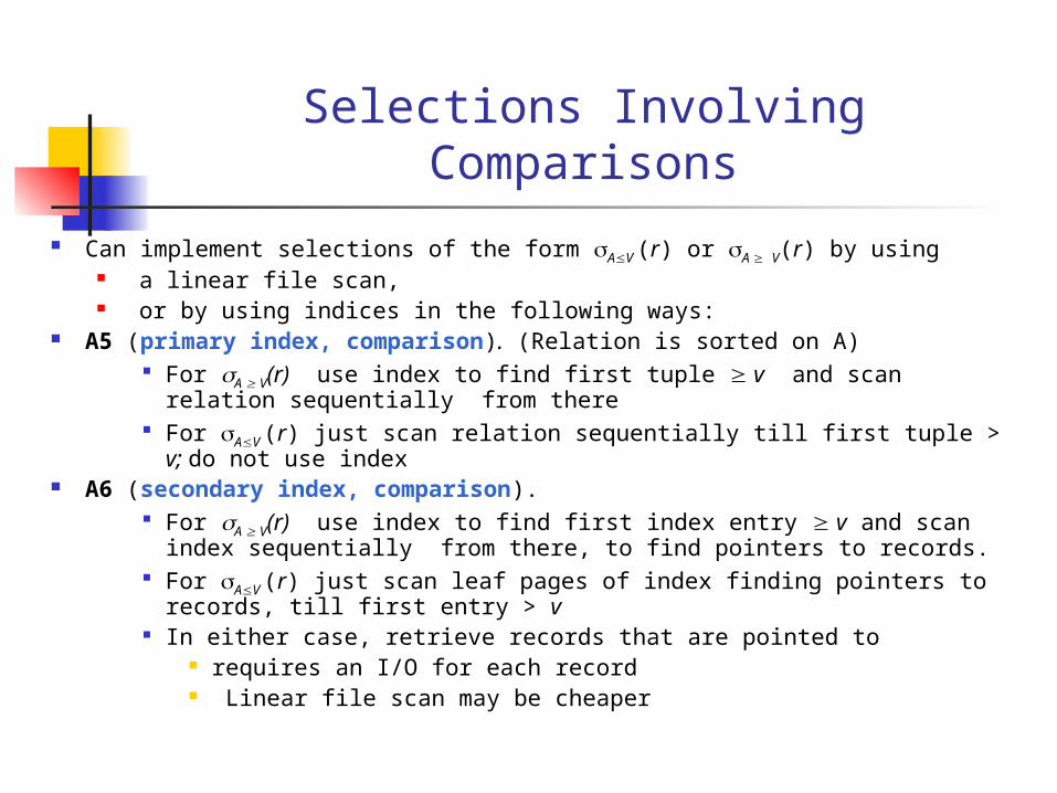
Selections Involving Comparisons

Can implement selections of the form AV (r) or A V(r) by using a linear file scan, or by using indices in the following ways:

A5 (primary index, comparison). (Relation is sorted on A) For A V(r) use index to find first tuple v and scan relation

sequentially from there For AV (r) just scan relation sequentially till first tuple > v; do not use

index A6 (secondary index, comparison).

For A V(r) use index to find first index entry v and scan index sequentially from there, to find pointers to records.

For AV (r) just scan leaf pages of index finding pointers to records, till first entry > v

In either case, retrieve records that are pointed to requires an I/O for each record Linear file scan may be cheaper

Implementation of Complex Selections

Conjunction: 1 2. . . n(r) A7 (conjunctive selection using one index).

Select a combination of i and algorithms A1 through A7 that results in the least cost for i (r).

Test other conditions on tuple after fetching it into memory buffer.

A8 (conjunctive selection using composite index). Use appropriate composite (multiple-key) index if available.

A9 (conjunctive selection by intersection of identifiers). Requires indices with record pointers. Use corresponding index for each condition, and take intersection

of all the obtained sets of record pointers. Then fetch records from file If some conditions do not have appropriate indices, apply test in

memory.

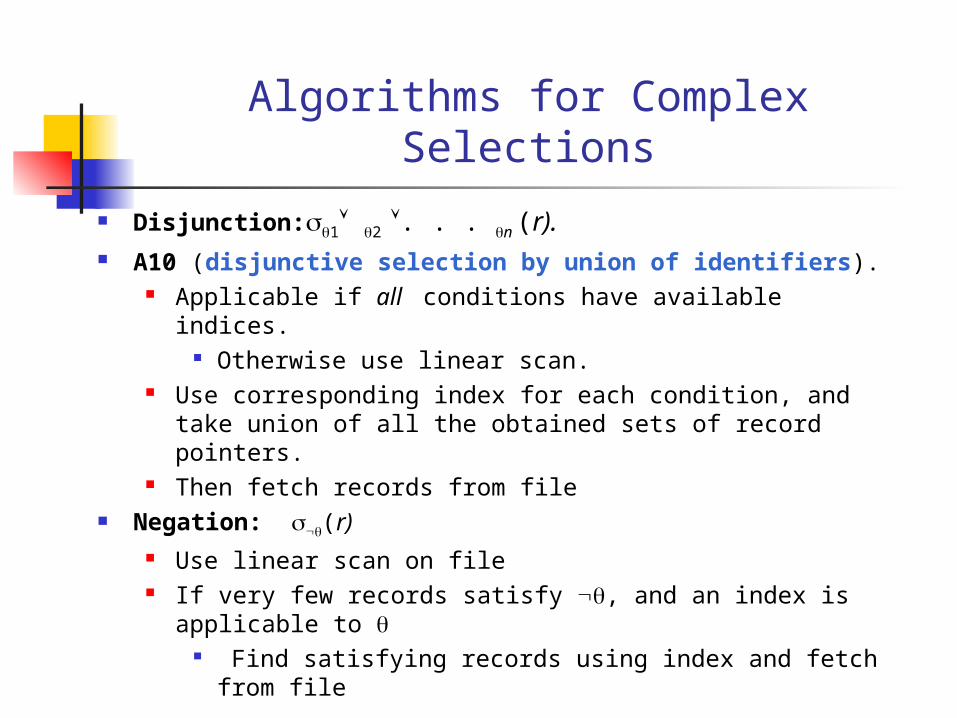
Algorithms for Complex Selections

Disjunction:1 2 . . . n (r). A10 (disjunctive selection by union of identifiers).

Applicable if all conditions have available indices. Otherwise use linear scan.

Use corresponding index for each condition, and take union of all the obtained sets of record pointers.

Then fetch records from file Negation: (r)

Use linear scan on file If very few records satisfy , and an index is applicable to

Find satisfying records using index and fetch from file

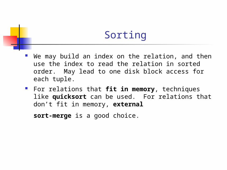
Sorting

We may build an index on the relation, and then use the index to read the relation in sorted order. May lead to one disk block access for each tuple.

For relations that fit in memory, techniques like quicksort can be used. For relations that don’t fit in memory, external

sort-merge is a good choice.

External Sort-MergeN-way Merge

1. Create sorted runs. Let i be 0 initially. Repeatedly do the following till the end of the relation: (a) Read M blocks of relation into memory (b) Sort the in-memory blocks (c) Write sorted data to run Ri; increment i.

Let the final value of i be N2. Merge the runs (next slide)…..

Let M denote memory size (in pages).

External Sort-Merge [2 of 3]

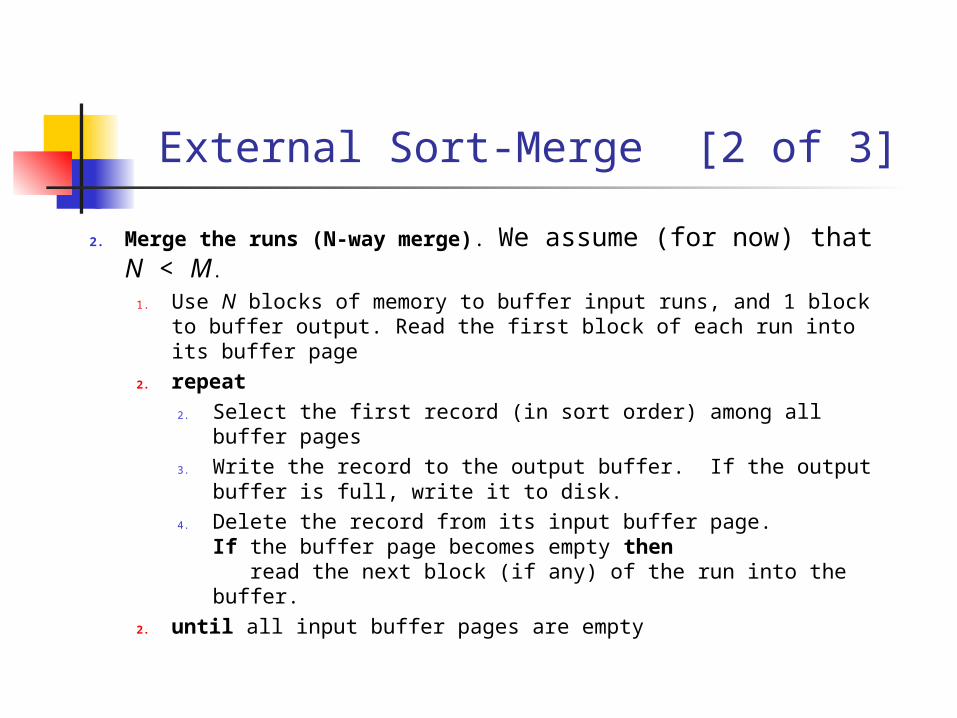
2. Merge the runs (N-way merge). We assume (for now) that N < M.

1. Use N blocks of memory to buffer input runs, and 1 block to buffer output. Read the first block of each run into its buffer page

2. repeat2. Select the first record (in sort order) among all buffer pages3. Write the record to the output buffer. If the output buffer is

full, write it to disk.4. Delete the record from its input buffer page.

If the buffer page becomes empty then read the next block (if any) of the run into the buffer.

2. until all input buffer pages are empty

External Sort-Merge [3 of 3]

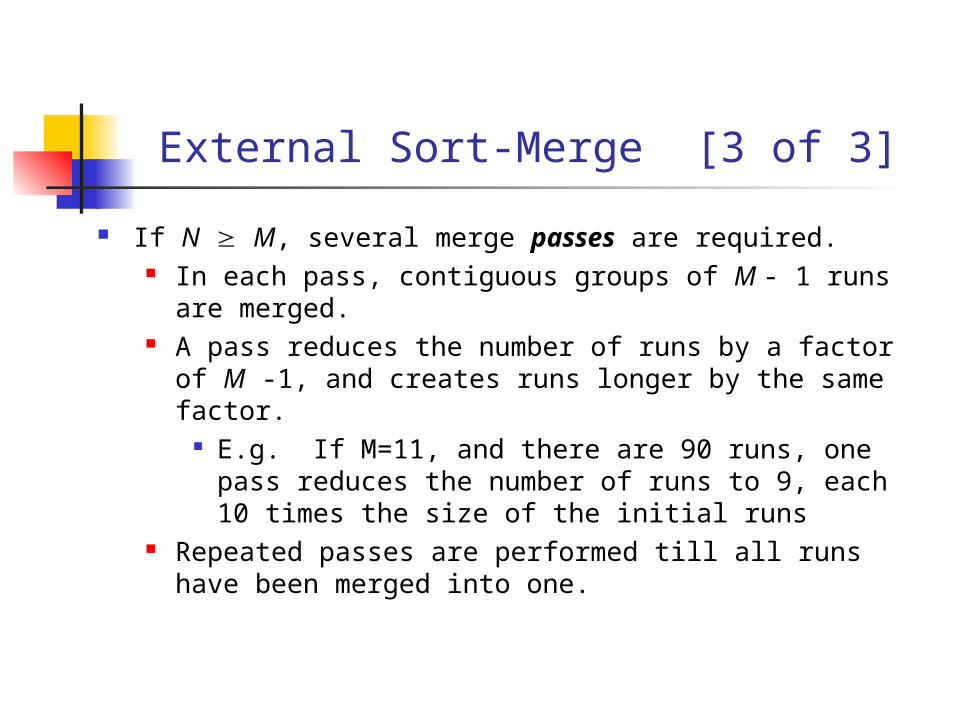
If N M, several merge passes are required. In each pass, contiguous groups of M - 1 runs are

merged. A pass reduces the number of runs by a factor of M -

1, and creates runs longer by the same factor. E.g. If M=11, and there are 90 runs, one pass

reduces the number of runs to 9, each 10 times the size of the initial runs

Repeated passes are performed till all runs have been merged into one.

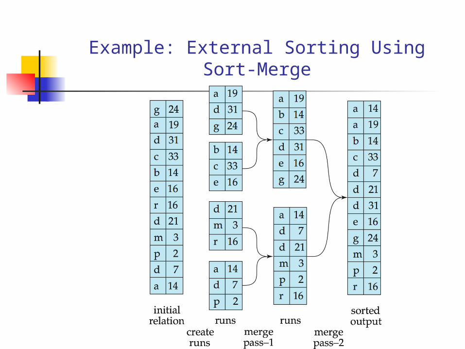
Example: External Sorting Using Sort-Merge

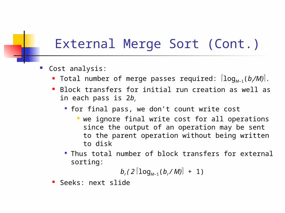
External Merge Sort (Cont.)

Cost analysis: Total number of merge passes required: logM–1(br/M). Block transfers for initial run creation as well as in each

pass is 2br

for final pass, we don’t count write cost we ignore final write cost for all operations since

the output of an operation may be sent to the parent operation without being written to disk

Thus total number of block transfers for external sorting:

br ( 2 logM–1(br / M) + 1) Seeks: next slide

External Merge Sort (Cont.)

Cost of seeks During run generation: one seek to read each run and

one seek to write each run 2 br / M

During the merge phase Buffer size: bb (read/write bb blocks at a time) Need 2 br / bb seeks for each merge pass

except the final one which does not require a write Total number of seeks:

2 br / M + br / bb (2 logM–1(br / M) -1)

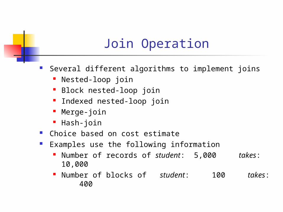
Join Operation

Several different algorithms to implement joins Nested-loop join Block nested-loop join Indexed nested-loop join Merge-join Hash-join

Choice based on cost estimate Examples use the following information

Number of records of student: 5,000 takes: 10,000 Number of blocks of student: 100 takes: 400

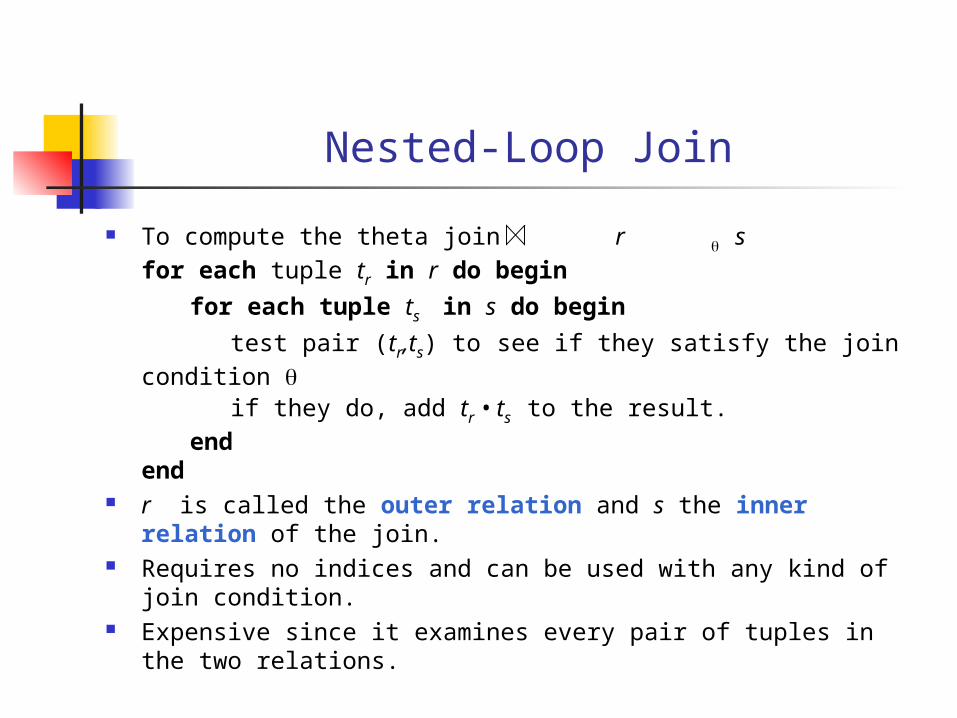
Nested-Loop Join

To compute the theta join r sfor each tuple tr in r do begin

for each tuple ts in s do begin

test pair (tr,ts) to see if they satisfy the join condition

if they do, add tr • ts to the result.end

end r is called the outer relation and s the inner relation of the

join. Requires no indices and can be used with any kind of join

condition. Expensive since it examines every pair of tuples in the two

relations.

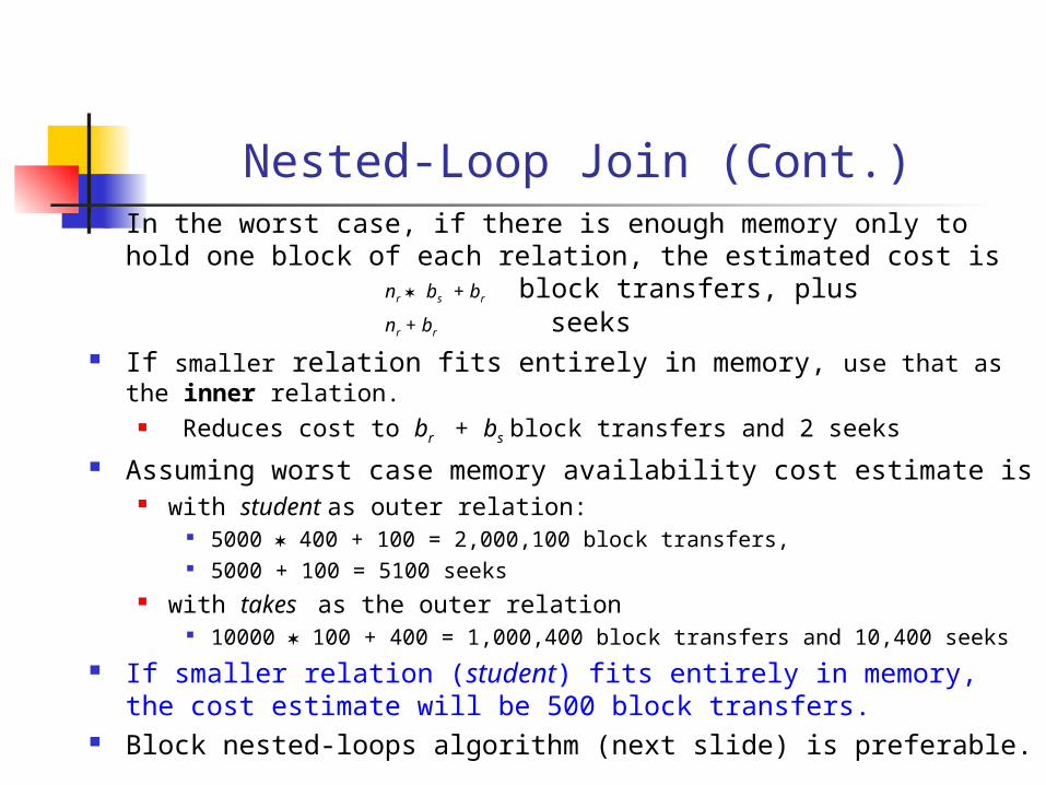
Nested-Loop Join (Cont.) In the worst case, if there is enough memory only to hold one

block of each relation, the estimated cost is nr bs + br block transfers, plus nr + br seeks

If smaller relation fits entirely in memory, use that as the inner relation.

Reduces cost to br + bs block transfers and 2 seeks

Assuming worst case memory availability cost estimate is with student as outer relation:

5000 400 + 100 = 2,000,100 block transfers, 5000 + 100 = 5100 seeks

with takes as the outer relation 10000 100 + 400 = 1,000,400 block transfers and 10,400 seeks

If smaller relation (student) fits entirely in memory, the cost estimate will be 500 block transfers.

Block nested-loops algorithm (next slide) is preferable.

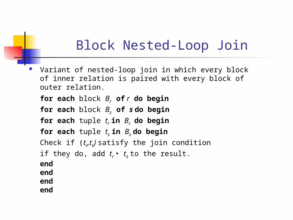
Block Nested-Loop Join

Variant of nested-loop join in which every block of inner relation is paired with every block of outer relation.

for each block Br of r do begin

for each block Bs of s do begin

for each tuple tr in Br do begin

for each tuple ts in Bs do begin

Check if (tr,ts) satisfy the join condition

if they do, add tr • ts to the result.

endend

endend

Block Nested-Loop Join (Cont.)

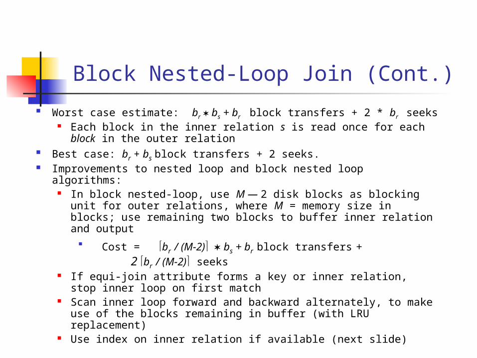
Worst case estimate: br bs + br block transfers + 2 * br seeks Each block in the inner relation s is read once for each block

in the outer relation Best case: br + bs block transfers + 2 seeks. Improvements to nested loop and block nested loop algorithms:

In block nested-loop, use M — 2 disk blocks as blocking unit for outer relations, where M = memory size in blocks; use remaining two blocks to buffer inner relation and output

Cost = br / (M-2) bs + br block transfers + 2 br / (M-2) seeks

If equi-join attribute forms a key or inner relation, stop inner loop on first match

Scan inner loop forward and backward alternately, to make use of the blocks remaining in buffer (with LRU replacement)

Use index on inner relation if available (next slide)

Merge-Join

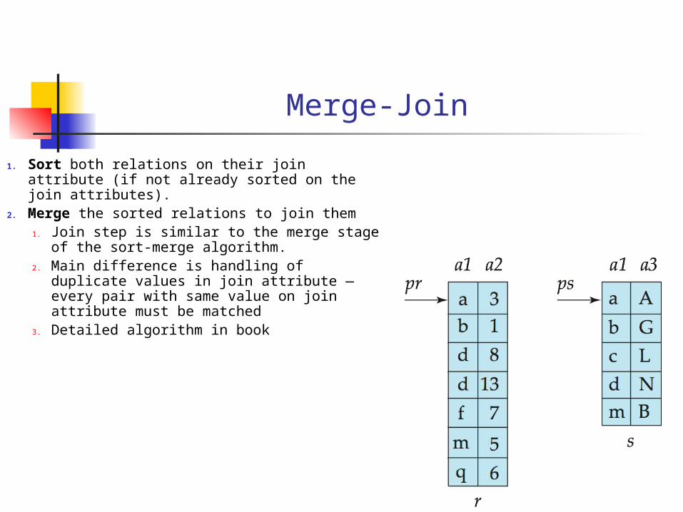
1. Sort both relations on their join attribute (if not already sorted on the join attributes).

2. Merge the sorted relations to join them1. Join step is similar to the merge stage of

the sort-merge algorithm. 2. Main difference is handling of duplicate

values in join attribute — every pair with same value on join attribute must be matched

3. Detailed algorithm in book

Merge-Join (Cont.)

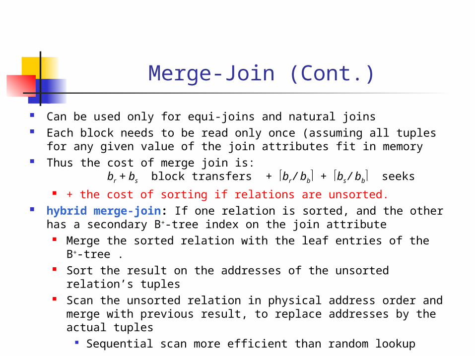
Can be used only for equi-joins and natural joins Each block needs to be read only once (assuming all tuples for any

given value of the join attributes fit in memory Thus the cost of merge join is:

br + bs block transfers + br / bb + bs / bb seeks + the cost of sorting if relations are unsorted.

hybrid merge-join: If one relation is sorted, and the other has a secondary B+-tree index on the join attribute

Merge the sorted relation with the leaf entries of the B+-tree . Sort the result on the addresses of the unsorted relation’s

tuples Scan the unsorted relation in physical address order and merge

with previous result, to replace addresses by the actual tuples Sequential scan more efficient than random lookup

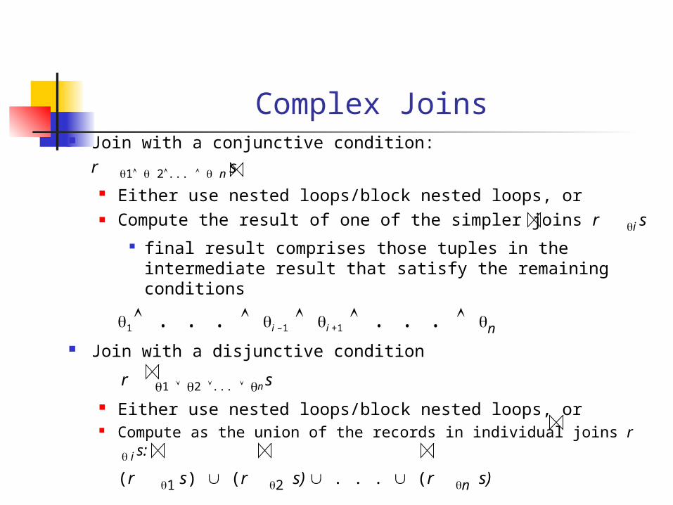
Complex Joins Join with a conjunctive condition:

r 1 2... n s Either use nested loops/block nested loops, or Compute the result of one of the simpler joins r i s

final result comprises those tuples in the intermediate result that satisfy the remaining conditions

1 . . . i –1 i +1 . . . n Join with a disjunctive condition

r 1 2 ... n s Either use nested loops/block nested loops, or Compute as the union of the records in individual joins r i s:

(r 1 s) (r 2 s) . . . (r n s)

Other Operations

Duplicate elimination can be implemented via hashing or sorting.

On sorting duplicates will come adjacent to each other, and all but one set of duplicates can be deleted.

Optimization: duplicates can be deleted during run generation as well as at intermediate merge steps in external sort-merge.

Hashing is similar – duplicates will come into the same bucket.

Projection: perform projection on each tuple followed by duplicate elimination.

Other Operations : Aggregation

Aggregation can be implemented in a manner similar to duplicate elimination.

Sorting or hashing can be used to bring tuples in the same group together, and then the aggregate functions can be applied on each group.

Optimization: combine tuples in the same group during run generation and intermediate merges, by computing partial aggregate values

For count, min, max, sum: keep aggregate values on tuples found so far in the group.

When combining partial aggregate for count, add up the aggregates

For avg, keep sum and count, and divide sum by count at the end

Evaluation of Expressions

So far: we have seen algorithms for individual operations

Alternatives for evaluating an entire expression tree Materialization: generate results of an expression

whose inputs are relations or are already computed, materialize (store) it on disk. Repeat.

Pipelining: pass on tuples to parent operations even as an operation is being executed

We study above alternatives in more detail

Materialization

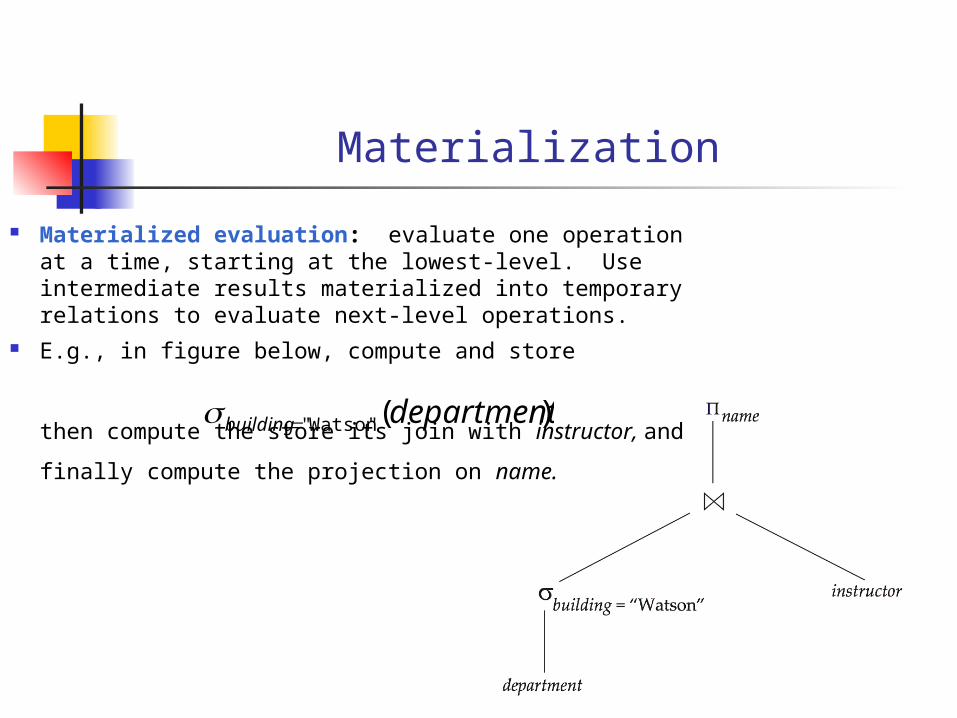
Materialized evaluation: evaluate one operation at a time, starting at the lowest-level. Use intermediate results materialized into temporary relations to evaluate next-level operations.

E.g., in figure below, compute and store

then compute the store its join with instructor, and

finally compute the projection on name.

)("Watson" departmentbuilding

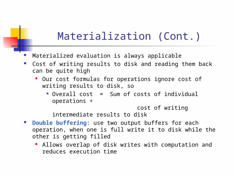
Materialization (Cont.)

Materialized evaluation is always applicable Cost of writing results to disk and reading them back can be

quite high Our cost formulas for operations ignore cost of writing

results to disk, so Overall cost = Sum of costs of individual operations +

cost of writing intermediate results to disk

Double buffering: use two output buffers for each operation, when one is full write it to disk while the other is getting filled

Allows overlap of disk writes with computation and reduces execution time

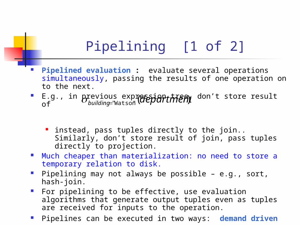
Pipelining [1 of 2]

Pipelined evaluation : evaluate several operations simultaneously, passing the results of one operation on to the next.

E.g., in previous expression tree, don’t store result of

instead, pass tuples directly to the join.. Similarly, don’t store

result of join, pass tuples directly to projection. Much cheaper than materialization: no need to store a temporary

relation to disk. Pipelining may not always be possible – e.g., sort, hash-join. For pipelining to be effective, use evaluation algorithms that

generate output tuples even as tuples are received for inputs to the operation.

Pipelines can be executed in two ways: demand driven and

producer driven

)("Watson" departmentbuilding

Pipelining [2 of 2]

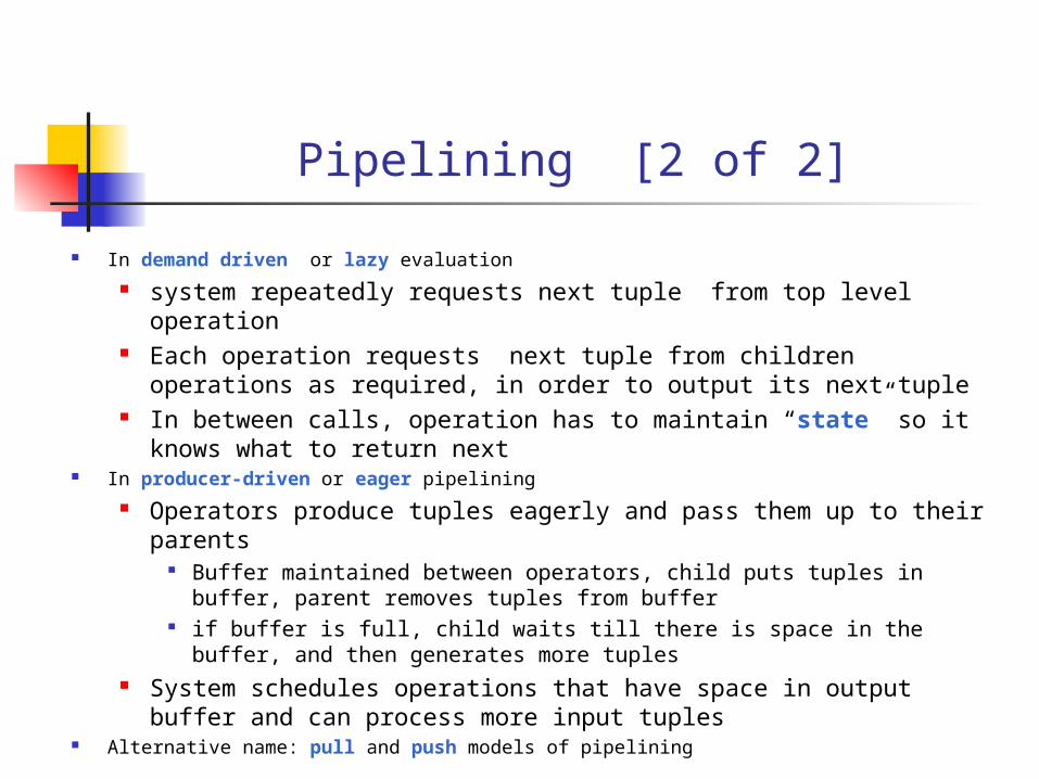
In demand driven or lazy evaluation system repeatedly requests next tuple from top level

operation Each operation requests next tuple from children operations

as required, in order to output its next tuple In between calls, operation has to maintain “state” so it knows

what to return next In producer-driven or eager pipelining

Operators produce tuples eagerly and pass them up to their parents

Buffer maintained between operators, child puts tuples in buffer, parent removes tuples from buffer

if buffer is full, child waits till there is space in the buffer, and then generates more tuples

System schedules operations that have space in output buffer and can process more input tuples

Alternative name: pull and push models of pipelining

CSc340 9b 40

Homework/Project

Homework due Next Class: 11.1, 11.3.b, 11.4 (6 pointers per node only), 11.6, 11.7,

11.9, 11.14 Homework due in One Week:

12.1, 12.2, 12.5, 12.6, 12.9

Project DEMO Next Class! Derek will bring MAC VGA Adapter…

Verify at least 5 tables, at least 50 tuples 3 or 4 SELECTs (JOINs, etc.) See Project Web Page for details A couple of UPDATEs Sample INSERT & DELETE "Front End"

CSc340 7a 41

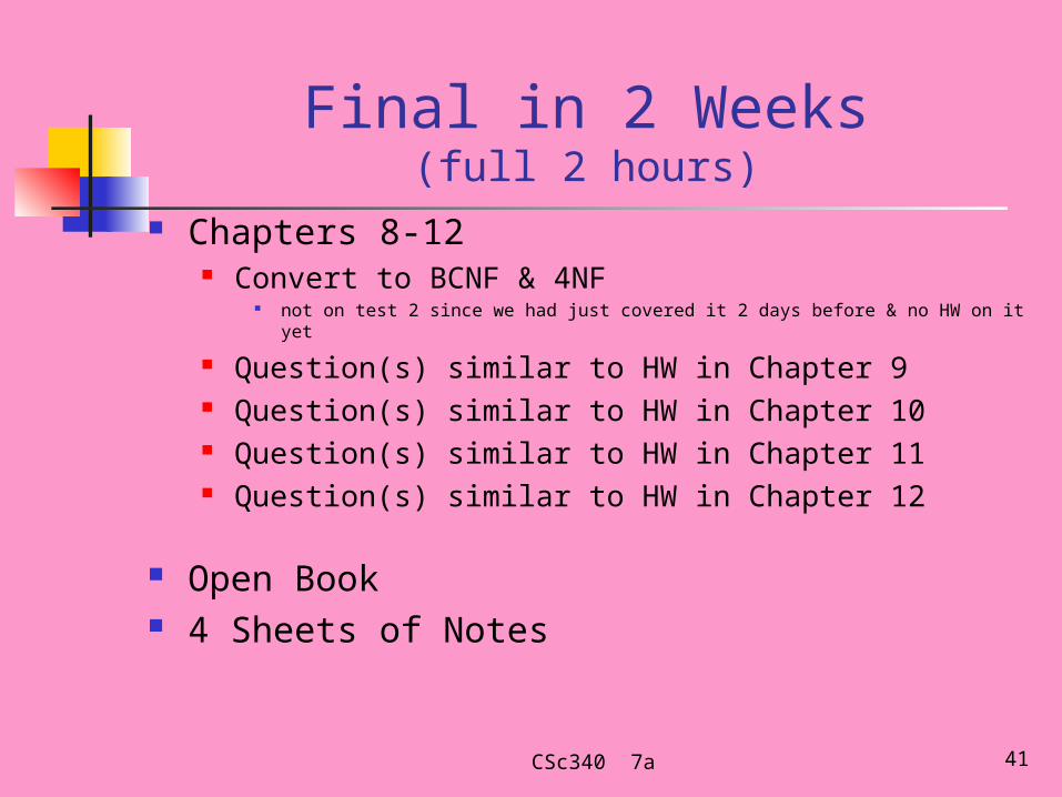
Final in 2 Weeks(full 2 hours)

Chapters 8-12 Convert to BCNF & 4NF

not on test 2 since we had just covered it 2 days before & no HW on it yet

Question(s) similar to HW in Chapter 9 Question(s) similar to HW in Chapter 10 Question(s) similar to HW in Chapter 11 Question(s) similar to HW in Chapter 12

Open Book 4 Sheets of Notes

CSc340 9b 42

In-Class Exercises(You may work together)

(See handout)

12.1 Sort-Merge Algorithm 12.2 Efficient Relational-Algebra

Expressions for Query

Lab Period

Class Project Senior Project if you need to!

CS Seminar @ 12:50 Grab some Lunch

Pizza outside room last time was NOT for us

CSc340 9b 43