csc 411: introduction to machine learningmren/teach/csc411_19s/... · csc 411: introduction to...

CSC 411: Introduction to Machine LearningLecture 3: Decision Trees

Mengye Ren and Matthew MacKay

University of Toronto

UofT CSC411 2019 Winter Lecture 03 1 / 34

Today

Decision Trees

I Simple but powerful learning algorithm

I One of the most widely used learning algorithms in Kaggle competitions

Lets us introduce ensembles (Lectures 4–5), a key idea in ML more broadly

Useful information theoretic concepts (entropy, mutual information, etc.)


Decision Trees

Decision trees make predictions by recursively splitting on differentattributes according to a tree structure.

Example: classifying fruit as an orange or lemon based on height and width

Yes No

Yes No Yes No


Decision Trees


Decision Trees

For continuous attributes, split based on less than or greater than somethreshold

Thus, input space is divided into regions with boundaries parallel to axes


Example with Discrete Inputs

What if the attributes are discrete?

Attributes:UofT CSC411 2019 Winter Lecture 03 6 / 34

Decision Tree: Example with Discrete Inputs

Possible tree to decide whether to wait (T) or not (F)


Decision Trees

Yes No

Yes No Yes No

Internal nodes test attributes

Branching is determined by attribute value

Leaf nodes are outputs (predictions)


Decision Tree: Classification and Regression

Each path from root to a leaf defines a region Rm

of input space

Let {(x (m1), t(m1)), . . . , (x (mk ), t(mk ))} be thetraining examples that fall into Rm

Classification tree:

I discrete output

I leaf value ym typically set to the most common value in{t(m1), . . . , t(mk )}

Regression tree:

I continuous output

I leaf value ym typically set to the mean value in {t(m1), . . . , t(mk )}

Note: We will focus on classification


How do we Learn a DecisionTree?

How do we construct a useful decision tree?


Learning Decision Trees

Learning the simplest (smallest) decision tree which correctly classifies training setis an NP complete problem [if you are interested, check: Hyafil & Rivest’76]

Resort to a greedy heuristic! Start with empty decision tree and completetraining set

I Split on the “best” attribute, i.e. partition datasetI Recurse on subpartitions

When should we stop?

Which attribute is the “best” (and where should we split, if continuous)?

I Choose based on accuracy?


Choosing a Good Split

Why isn’t accuracy a good measure?

Is this split good? Zero accuracy gain.

But we’ve reduced our uncertainty about whether a fruit is a lemon


Choosing a Good Split

How can we quantify uncertainty in prediction for a given leaf node?

I All examples in leaf have same class: good, low uncertaintyI Each class has same amount of examples in leaf: bad, high uncertainty

Idea: Use counts at leaves to define probability distributions, and useinformation theory to measure uncertainty


We Flip Two Different Coins

Sequence 1: 0 0 0 1 0 0 0 0 0 0 0 0 0 0 0 1 0 0 ... ?

Sequence 2: 0 1 0 1 0 1 1 1 0 1 0 0 1 1 0 1 0 1 ... ?

16

2 8 10

0 1

versus

0 1


Quantifying Uncertainty

Entropy is a measure of expected “surprise”: How uncertain are we of the valueof a draw from this distribution?

H(X ) = −∑x∈X

p(x) log2 p(x)

0 1

8/9

1/9

−8

9log2

8

9− 1

9log2

1

9≈ 1

2

0 1

4/9 5/9

−4

9log2

4

9− 5

9log2

5

9≈ 0.99

Averages over information content of each observation

Unit = bits

A fair coin flip has 1 bit of entropyUofT CSC411 2019 Winter Lecture 03 15 / 34

Quantifying Uncertainty

H(X ) = −∑x∈X

p(x) log2 p(x)

0.2 0.4 0.6 0.8 1.0probability p of heads

0.2

0.4

0.6

0.8

1.0

entropy


Entropy

“High Entropy”:

I Variable has a uniform like distributionI Flat histogramI Values sampled from it are less predictable

“Low Entropy”

I Distribution of variable has peaks and valleysI Histogram has lows and highsI Values sampled from it are more predictable

[Slide credit: Vibhav Gogate]


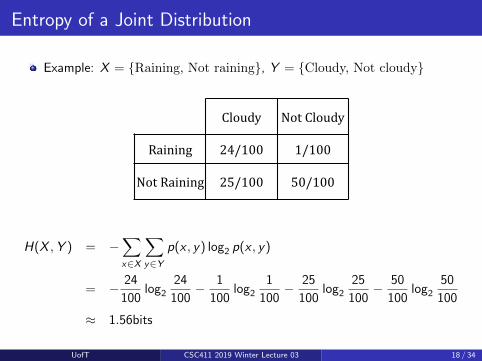
Entropy of a Joint Distribution

Example: X = {Raining, Not raining}, Y = {Cloudy, Not cloudy}

Cloudy' Not'Cloudy'

Raining' 24/100' 1/100'

Not'Raining' 25/100' 50/100'

H(X ,Y ) = −∑x∈X

∑y∈Y

p(x , y) log2 p(x , y)

= − 24

100log2

24

100− 1

100log2

1

100− 25

100log2

25

100− 50

100log2

50

100

≈ 1.56bits


Specific Conditional Entropy


Cloudy' Not'Cloudy'

Raining' 24/100' 1/100'

Not'Raining' 25/100' 50/100'

What is the entropy of cloudiness Y , given that it is raining?

H(Y |X = raining) = −∑y∈Y

p(y |raining) log2 p(y |raining)

= −24

25log2

24

25− 1

25log2

1

25

≈ 0.24bits

We used: p(y |x) = p(x,y)p(x) , and p(x) =

∑y p(x , y) (sum in a row)


Conditional Entropy

Cloudy' Not'Cloudy'

Raining' 24/100' 1/100'

Not'Raining' 25/100' 50/100'

The expected conditional entropy:

H(Y |X ) = Ex∼p(x)[H(Y |X = x)] (1)

=∑x∈X

p(x)H(Y |X = x)

= −∑x∈X

∑y∈Y

p(x , y) log2 p(y |x)


Conditional Entropy


Cloudy' Not'Cloudy'

Raining' 24/100' 1/100'

Not'Raining' 25/100' 50/100'

What is the entropy of cloudiness, given the knowledge of whether or not itis raining?

H(Y |X ) =∑x∈X

p(x)H(Y |X = x)

=1

4H(cloudy|is raining) +

3

4H(cloudy|not raining)

≈ 0.75 bits


Conditional Entropy

Some useful properties:

I H is always non-negative

I Chain rule: H(X ,Y ) = H(X |Y ) + H(Y ) = H(Y |X ) + H(X )

I If X and Y independent, then X doesn’t tell us anything about Y :H(Y |X ) = H(Y )

I But Y tells us everything about Y : H(Y |Y ) = 0

I By knowing X , we can only decrease uncertainty about Y :H(Y |X ) ≤ H(Y )


Information Gain

Cloudy' Not'Cloudy'

Raining' 24/100' 1/100'

Not'Raining' 25/100' 50/100'

How much information about cloudiness do we get by discovering whether itis raining?

IG (Y |X ) = H(Y )− H(Y |X )

≈ 0.25 bits

This is called the information gain in Y due to X , or the mutualinformation of Y and X

If X is completely uninformative about Y : IG (Y |X ) = 0

If X is completely informative about Y : IG (Y |X ) = H(Y )


Revisiting Our Original Example

Information gain measures the informativeness of a variable, which is exactlywhat we desire in a decision tree attribute!

What is the information gain of this split?

Let Y be r.v. denoting lemon or orange, B be r.v. denoting whether left orright split taken

Root entropy: H(Y ) = − 49149 log2( 49

149 )− 100149 log2( 100

149 ) ≈ 0.91

Leafs entropy: H(Y |B = left) = 0, H(Y |B = right) ≈ 1.

IG (Y |B) ≈ 0.91− ( 13 · 0 + 2

3 · 1) ≈ 0.24 > 0


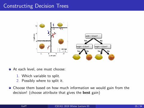
Constructing Decision Trees

Yes No

Yes No Yes No

At each level, one must choose:

1. Which variable to split.2. Possibly where to split it.

Choose them based on how much information we would gain from thedecision! (choose attribute that gives the best gain)


Decision Tree Construction Algorithm

Simple, greedy, recursive approach, builds up tree node-by-node

Start with empty decision tree and complete training set

I Split on the most informative attribute, partitioning datasetI Recurse on subpartitions

Possible termination condition: end if all examples in current subpartitionshare the same class


Back to Our Example

Attributes: [from: Russell & Norvig]


Which Tree is Better?


What Makes a Good Tree?

Not too small: need to handle important but possibly subtle distinctions indata

Not too big:

I Computational efficiency (avoid redundant, spurious attributes)I Avoid over-fitting training examplesI Human interpretability

“Occam’s Razor”: find the simplest hypothesis that fits the observations

I Useful principle, but hard to formalize (how to define simplicity?)I See Domingos, 1999, “The role of Occam’s razor in knowledge

discovery”

We desire small trees with informative nodes near the root


Expressiveness

Discrete-input, discrete-output case:

I Decision trees can express any function of the input attributesI E.g., for Boolean functions, truth table row → path to leaf:

Continuous-input, continuous-output case:

I Can approximate any function arbitrarily closely

Trivially, there is a consistent decision tree for any training set w/ one pathto leaf for each example (unless f nondeterministic in x) but it probablywon’t generalize to new examples

[Slide credit: S. Russell]


Decision Tree Miscellany

Problems:

I You have exponentially less data at lower levelsI Too big of a tree can overfit the dataI Greedy algorithms don’t necessarily yield the global optimumI Mistakes at top-level propagate down tree

Handling continuous attributes

I Split based on a threshold, chosen to maximize information gain

Decision trees can also be used for regression on real-valued outputs. Choosesplits to minimize squared error, rather than maximize information gain.


Comparison to k-NN

Advantages of decision trees over k-NN

Good with discrete attributes

Easily deals with missing values (just treat as another value)

Robust to scale of inputs- only depends on ordering

Fast at test time

More interpretable


Comparison to k-NN

Advantages of k-NN over decision trees

Able to handle attributes/features that interact in complex ways(e.g. pixels)

Can incorporate interesting distance measures (e.g. shape contexts)

Typically make better predictions in practiceI As we’ll see next lecture, ensembles of decision trees are much

stronger. But they lose many of the advantages listed above.


csc 411: introduction to machine learningmren/teach/csc411_19s/... · csc 411: introduction to...

Documents