crystal ball tutorials
TRANSCRIPT

O R A C L E ® C R Y S T A L B A L L , F U S I O N E D I T I O N
R E L E A S E 1 1 . 1 . 1 . 3 . 0 0
U S E R ' S G U I D E

Crystal Ball User's Guide, 11.1.1.3.00
Copyright © 1988, 2009, Oracle and/or its affiliates. All rights reserved.
Authors: EPM Information Development Team
The Programs (which include both the software and documentation) contain proprietary information; they are providedunder a license agreement containing restrictions on use and disclosure and are also protected by copyright, patent, andother intellectual and industrial property laws. Reverse engineering, disassembly, or decompilation of the Programs, exceptto the extent required to obtain interoperability with other independently created software or as specified by law, isprohibited.
The information contained in this document is subject to change without notice. If you find any problems in thedocumentation, please report them to us in writing. This document is not warranted to be error-free. Except as may beexpressly permitted in your license agreement for these Programs, no part of these Programs may be reproduced ortransmitted in any form or by any means, electronic or mechanical, for any purpose.
If the Programs are delivered to the United States Government or anyone licensing or using the Programs on behalf of theUnited States Government, the following notice is applicable:
U.S. GOVERNMENT RIGHTS Programs, software, databases, and related documentation and technical data delivered toU.S. Government customers are "commercial computer software" or "commercial technical data" pursuant to theapplicable Federal Acquisition Regulation and agency-specific supplemental regulations. As such, use, duplication,disclosure, modification, and adaptation of the Programs, including documentation and technical data, shall be subjectto the licensing restrictions set forth in the applicable Oracle license agreement, and, to the extent applicable, the additionalrights set forth in FAR 52.227-19, Commercial Computer Software--Restricted Rights (June 1987). Oracle USA, Inc., 500Oracle Parkway, Redwood City, CA 94065.
The Programs are not intended for use in any nuclear, aviation, mass transit, medical, or other inherently dangerousapplications. It shall be the licensee's responsibility to take all appropriate fail-safe, backup, redundancy and other measuresto ensure the safe use of such applications if the Programs are used for such purposes, and we disclaim liability for anydamages caused by such use of the Programs.
Oracle, JD Edwards, PeopleSoft, and Siebel are registered trademarks of Oracle Corporation and/or its affiliates. Othernames may be trademarks of their respective owners.
The Programs may provide links to Web sites and access to content, products, and services from third parties. Oracle isnot responsible for the availability of, or any content provided on, third-party Web sites. You bear all risks associated withthe use of such content. If you choose to purchase any products or services from a third party, the relationship is directlybetween you and the third party. Oracle is not responsible for: (a) the quality of third-party products or services; or (b)fulfilling any of the terms of the agreement with the third party, including delivery of products or services and warrantyobligations related to purchased products or services. Oracle is not responsible for any loss or damage of any sort that youmay incur from dealing with any third party.
Contents
Chapter 1. Welcome . . . . . . . . . . . . . . . . . . . . . . . . . . . . . . . . . . . . . . . . . . . . . . . . . . . . . . . . . . . . . . . . 13
Introduction . . . . . . . . . . . . . . . . . . . . . . . . . . . . . . . . . . . . . . . . . . . . . . . . . . . . . . . . . 13
Who Should Use This Program . . . . . . . . . . . . . . . . . . . . . . . . . . . . . . . . . . . . . . . . . . . 14
What You Will Need . . . . . . . . . . . . . . . . . . . . . . . . . . . . . . . . . . . . . . . . . . . . . . . . . . . 14
About the Crystal Ball Documentation Set . . . . . . . . . . . . . . . . . . . . . . . . . . . . . . . . . . . 14
Screen Capture Notes . . . . . . . . . . . . . . . . . . . . . . . . . . . . . . . . . . . . . . . . . . . . . . . 16
Getting Help . . . . . . . . . . . . . . . . . . . . . . . . . . . . . . . . . . . . . . . . . . . . . . . . . . . . . . . . . 16
Technical Support and More . . . . . . . . . . . . . . . . . . . . . . . . . . . . . . . . . . . . . . . . . . . . . 16
Chapter 2. Crystal Ball Overview . . . . . . . . . . . . . . . . . . . . . . . . . . . . . . . . . . . . . . . . . . . . . . . . . . . . . . . 17
Introduction . . . . . . . . . . . . . . . . . . . . . . . . . . . . . . . . . . . . . . . . . . . . . . . . . . . . . . . . . 17
Model Building and Risk Analysis Overview . . . . . . . . . . . . . . . . . . . . . . . . . . . . . . . . . . 17
What is a Model? . . . . . . . . . . . . . . . . . . . . . . . . . . . . . . . . . . . . . . . . . . . . . . . . . . 18
Risk and Certainty . . . . . . . . . . . . . . . . . . . . . . . . . . . . . . . . . . . . . . . . . . . . . . . . . 18
How Crystal Ball Differs from Traditional Analysis Tools . . . . . . . . . . . . . . . . . . . . . 19
Monte Carlo Simulation and Crystal Ball . . . . . . . . . . . . . . . . . . . . . . . . . . . . . . . . . 20
Crystal Ball Feature Overview . . . . . . . . . . . . . . . . . . . . . . . . . . . . . . . . . . . . . . . . . . . . 22
Charts and Analysis Tools . . . . . . . . . . . . . . . . . . . . . . . . . . . . . . . . . . . . . . . . . . . . 22
Other Crystal Ball Tools . . . . . . . . . . . . . . . . . . . . . . . . . . . . . . . . . . . . . . . . . . . . . 29
Process Capability Features . . . . . . . . . . . . . . . . . . . . . . . . . . . . . . . . . . . . . . . . . . . 31
Trend Analysis with Predictor . . . . . . . . . . . . . . . . . . . . . . . . . . . . . . . . . . . . . . . . . 31
Optimizing Decision Variable Values with OptQuest . . . . . . . . . . . . . . . . . . . . . . . . 31
Steps for Using Crystal Ball . . . . . . . . . . . . . . . . . . . . . . . . . . . . . . . . . . . . . . . . . . . . . . 31
Resources for Learning Crystal Ball . . . . . . . . . . . . . . . . . . . . . . . . . . . . . . . . . . . . . 32
Starting and Closing Crystal Ball . . . . . . . . . . . . . . . . . . . . . . . . . . . . . . . . . . . . . . . . . . 32
Starting Crystal Ball Manually . . . . . . . . . . . . . . . . . . . . . . . . . . . . . . . . . . . . . . . . . 32
Starting Crystal Ball Automatically . . . . . . . . . . . . . . . . . . . . . . . . . . . . . . . . . . . . . . 33
Crystal Ball Welcome Screen . . . . . . . . . . . . . . . . . . . . . . . . . . . . . . . . . . . . . . . . . . 33
Closing Crystal Ball . . . . . . . . . . . . . . . . . . . . . . . . . . . . . . . . . . . . . . . . . . . . . . . . . 34
Crystal Ball Menus and Toolbar . . . . . . . . . . . . . . . . . . . . . . . . . . . . . . . . . . . . . . . . . . . 34
The Crystal Ball Menus . . . . . . . . . . . . . . . . . . . . . . . . . . . . . . . . . . . . . . . . . . . . . . 34
The Crystal Ball Toolbar . . . . . . . . . . . . . . . . . . . . . . . . . . . . . . . . . . . . . . . . . . . . . 35
Contents iii
Crystal Ball Tutorials . . . . . . . . . . . . . . . . . . . . . . . . . . . . . . . . . . . . . . . . . . . . . . . . . . . 35
Chapter 3. Defining Model Assumptions . . . . . . . . . . . . . . . . . . . . . . . . . . . . . . . . . . . . . . . . . . . . . . . . . . 37
Introduction . . . . . . . . . . . . . . . . . . . . . . . . . . . . . . . . . . . . . . . . . . . . . . . . . . . . . . . . . 37
Types of Data Cells . . . . . . . . . . . . . . . . . . . . . . . . . . . . . . . . . . . . . . . . . . . . . . . . . . . . 37
About Assumptions and Probability Distributions . . . . . . . . . . . . . . . . . . . . . . . . . . . . . 38
Defining Assumptions . . . . . . . . . . . . . . . . . . . . . . . . . . . . . . . . . . . . . . . . . . . . . . . . . . 38
Entering Assumptions . . . . . . . . . . . . . . . . . . . . . . . . . . . . . . . . . . . . . . . . . . . . . . . . . . 38
Additional Assumption Features . . . . . . . . . . . . . . . . . . . . . . . . . . . . . . . . . . . . . . . . . . 41
Entering Cell References and Formulas . . . . . . . . . . . . . . . . . . . . . . . . . . . . . . . . . . 42
Alternate Parameter Sets . . . . . . . . . . . . . . . . . . . . . . . . . . . . . . . . . . . . . . . . . . . . . 43
Fitting Distributions to Data . . . . . . . . . . . . . . . . . . . . . . . . . . . . . . . . . . . . . . . . . . 44
Specifying Correlations Between Assumptions . . . . . . . . . . . . . . . . . . . . . . . . . . . . . 47
Setting Assumption Preferences . . . . . . . . . . . . . . . . . . . . . . . . . . . . . . . . . . . . . . . . 50
Using the Crystal Ball Distribution Gallery . . . . . . . . . . . . . . . . . . . . . . . . . . . . . . . . . . . 51
Displaying the Distribution Gallery . . . . . . . . . . . . . . . . . . . . . . . . . . . . . . . . . . . . . 51
Distribution Gallery Window . . . . . . . . . . . . . . . . . . . . . . . . . . . . . . . . . . . . . . . . . 51
Managing Distributions . . . . . . . . . . . . . . . . . . . . . . . . . . . . . . . . . . . . . . . . . . . . . 53
Managing Categories . . . . . . . . . . . . . . . . . . . . . . . . . . . . . . . . . . . . . . . . . . . . . . . . 57
Chapter 4. Defining Other Model Elements . . . . . . . . . . . . . . . . . . . . . . . . . . . . . . . . . . . . . . . . . . . . . . . . 63
Introduction . . . . . . . . . . . . . . . . . . . . . . . . . . . . . . . . . . . . . . . . . . . . . . . . . . . . . . . . . 63
Defining Decision Variable Cells . . . . . . . . . . . . . . . . . . . . . . . . . . . . . . . . . . . . . . . . . . 63
Defining Forecasts . . . . . . . . . . . . . . . . . . . . . . . . . . . . . . . . . . . . . . . . . . . . . . . . . . . . 64
Setting Forecast Preferences . . . . . . . . . . . . . . . . . . . . . . . . . . . . . . . . . . . . . . . . . . . 65
Working with Crystal Ball Data . . . . . . . . . . . . . . . . . . . . . . . . . . . . . . . . . . . . . . . . . . . 68
Editing Crystal Ball Data . . . . . . . . . . . . . . . . . . . . . . . . . . . . . . . . . . . . . . . . . . . . . 68
Selecting and Reviewing Data . . . . . . . . . . . . . . . . . . . . . . . . . . . . . . . . . . . . . . . . . 70
Setting Cell Preferences . . . . . . . . . . . . . . . . . . . . . . . . . . . . . . . . . . . . . . . . . . . . . . . . . 72
Saving and Restoring Models . . . . . . . . . . . . . . . . . . . . . . . . . . . . . . . . . . . . . . . . . . . . . 73
Chapter 5. Running Simulations . . . . . . . . . . . . . . . . . . . . . . . . . . . . . . . . . . . . . . . . . . . . . . . . . . . . . . . . 75
Introduction . . . . . . . . . . . . . . . . . . . . . . . . . . . . . . . . . . . . . . . . . . . . . . . . . . . . . . . . . 75
About Crystal Ball Simulations . . . . . . . . . . . . . . . . . . . . . . . . . . . . . . . . . . . . . . . . . . . 75
Setting Run Preferences . . . . . . . . . . . . . . . . . . . . . . . . . . . . . . . . . . . . . . . . . . . . . . . . 76
Setting Trials Preferences . . . . . . . . . . . . . . . . . . . . . . . . . . . . . . . . . . . . . . . . . . . . . 76
Setting Sampling Preferences . . . . . . . . . . . . . . . . . . . . . . . . . . . . . . . . . . . . . . . . . . 77
Setting Speed Preferences . . . . . . . . . . . . . . . . . . . . . . . . . . . . . . . . . . . . . . . . . . . . 78
Setting Options Preferences . . . . . . . . . . . . . . . . . . . . . . . . . . . . . . . . . . . . . . . . . . . 79
Setting Statistics Preferences . . . . . . . . . . . . . . . . . . . . . . . . . . . . . . . . . . . . . . . . . . 80
iv Contents
Freezing Crystal Ball Data Cells . . . . . . . . . . . . . . . . . . . . . . . . . . . . . . . . . . . . . . . . . . . 80
Running Simulations . . . . . . . . . . . . . . . . . . . . . . . . . . . . . . . . . . . . . . . . . . . . . . . . . . 81
Starting Simulations . . . . . . . . . . . . . . . . . . . . . . . . . . . . . . . . . . . . . . . . . . . . . . . . 81
Stopping Simulations . . . . . . . . . . . . . . . . . . . . . . . . . . . . . . . . . . . . . . . . . . . . . . . 82
Continuing Simulations . . . . . . . . . . . . . . . . . . . . . . . . . . . . . . . . . . . . . . . . . . . . . 82
Resetting and Rerunning Simulations . . . . . . . . . . . . . . . . . . . . . . . . . . . . . . . . . . . . 82
Single-Stepping . . . . . . . . . . . . . . . . . . . . . . . . . . . . . . . . . . . . . . . . . . . . . . . . . . . . 82
The Crystal Ball Control Panel . . . . . . . . . . . . . . . . . . . . . . . . . . . . . . . . . . . . . . . . . 83
Managing Chart Windows . . . . . . . . . . . . . . . . . . . . . . . . . . . . . . . . . . . . . . . . . . . . . . . 84
Single Windows . . . . . . . . . . . . . . . . . . . . . . . . . . . . . . . . . . . . . . . . . . . . . . . . . . . 84
Multiple Windows . . . . . . . . . . . . . . . . . . . . . . . . . . . . . . . . . . . . . . . . . . . . . . . . . 84
Saving and Restoring Simulation Results . . . . . . . . . . . . . . . . . . . . . . . . . . . . . . . . . . . . 86
Saving Crystal Ball Simulation Results . . . . . . . . . . . . . . . . . . . . . . . . . . . . . . . . . . . 86
Restoring Crystal Ball Simulation Results . . . . . . . . . . . . . . . . . . . . . . . . . . . . . . . . . 87
Using Restored Results . . . . . . . . . . . . . . . . . . . . . . . . . . . . . . . . . . . . . . . . . . . . . . 87
Restored Results with Capability Metrics . . . . . . . . . . . . . . . . . . . . . . . . . . . . . . . . . 87
Functions for Use in Excel Models . . . . . . . . . . . . . . . . . . . . . . . . . . . . . . . . . . . . . . . . . 88
Running User-Defined Macros . . . . . . . . . . . . . . . . . . . . . . . . . . . . . . . . . . . . . . . . . . . 88
User-Defined Macro Interfaces . . . . . . . . . . . . . . . . . . . . . . . . . . . . . . . . . . . . . . . . 89
Priority Rules . . . . . . . . . . . . . . . . . . . . . . . . . . . . . . . . . . . . . . . . . . . . . . . . . . . . . 91
Global Macros . . . . . . . . . . . . . . . . . . . . . . . . . . . . . . . . . . . . . . . . . . . . . . . . . . . . 91
Toolbar Macros . . . . . . . . . . . . . . . . . . . . . . . . . . . . . . . . . . . . . . . . . . . . . . . . . . . 92
Chapter 6. Analyzing Forecast Charts . . . . . . . . . . . . . . . . . . . . . . . . . . . . . . . . . . . . . . . . . . . . . . . . . . . . 93
Introduction . . . . . . . . . . . . . . . . . . . . . . . . . . . . . . . . . . . . . . . . . . . . . . . . . . . . . . . . . 93
Guidelines for Analyzing Simulation Results . . . . . . . . . . . . . . . . . . . . . . . . . . . . . . . . . . 93
Understanding and Using Forecast Charts . . . . . . . . . . . . . . . . . . . . . . . . . . . . . . . . . . . 95
Determining the Certainty Level . . . . . . . . . . . . . . . . . . . . . . . . . . . . . . . . . . . . . . . 96
Focusing On the Display Range . . . . . . . . . . . . . . . . . . . . . . . . . . . . . . . . . . . . . . . 100
Formatting Chart Numbers . . . . . . . . . . . . . . . . . . . . . . . . . . . . . . . . . . . . . . . . . . 101
Changing the Distribution View and Interpreting Statistics . . . . . . . . . . . . . . . . . . . 102
Setting Forecast Preferences . . . . . . . . . . . . . . . . . . . . . . . . . . . . . . . . . . . . . . . . . . 110
Setting Forecast Chart Preferences . . . . . . . . . . . . . . . . . . . . . . . . . . . . . . . . . . . . . 111
Setting Chart Preferences . . . . . . . . . . . . . . . . . . . . . . . . . . . . . . . . . . . . . . . . . . . . . . . 112
Setting Preferences with Shortcut Keys . . . . . . . . . . . . . . . . . . . . . . . . . . . . . . . . . . 112
Basic Customization Instructions . . . . . . . . . . . . . . . . . . . . . . . . . . . . . . . . . . . . . . 113
Specific Customization Instructions . . . . . . . . . . . . . . . . . . . . . . . . . . . . . . . . . . . . 114
Managing Existing Charts . . . . . . . . . . . . . . . . . . . . . . . . . . . . . . . . . . . . . . . . . . . . . . 121
Opening Charts . . . . . . . . . . . . . . . . . . . . . . . . . . . . . . . . . . . . . . . . . . . . . . . . . . 121
Contents v

Copying and Pasting Charts to Other Applications . . . . . . . . . . . . . . . . . . . . . . . . . 122
Printing Charts . . . . . . . . . . . . . . . . . . . . . . . . . . . . . . . . . . . . . . . . . . . . . . . . . . . 123
Closing Charts . . . . . . . . . . . . . . . . . . . . . . . . . . . . . . . . . . . . . . . . . . . . . . . . . . . 123
Deleting Charts . . . . . . . . . . . . . . . . . . . . . . . . . . . . . . . . . . . . . . . . . . . . . . . . . . . 124
Chapter 7. Analyzing Other Charts . . . . . . . . . . . . . . . . . . . . . . . . . . . . . . . . . . . . . . . . . . . . . . . . . . . . . 125
Overview . . . . . . . . . . . . . . . . . . . . . . . . . . . . . . . . . . . . . . . . . . . . . . . . . . . . . . . . . . 125
Selecting Assumptions, Forecasts, and other Data Types . . . . . . . . . . . . . . . . . . . . . 126
Understanding and Using Overlay Charts . . . . . . . . . . . . . . . . . . . . . . . . . . . . . . . . . . . 126
Creating Overlay Charts . . . . . . . . . . . . . . . . . . . . . . . . . . . . . . . . . . . . . . . . . . . . 127
Customizing Overlay Charts . . . . . . . . . . . . . . . . . . . . . . . . . . . . . . . . . . . . . . . . . 130
Using Distribution Fitting with Overlay Charts . . . . . . . . . . . . . . . . . . . . . . . . . . . . 130
Understanding and Using Trend Charts . . . . . . . . . . . . . . . . . . . . . . . . . . . . . . . . . . . . 131
Creating Trend Charts . . . . . . . . . . . . . . . . . . . . . . . . . . . . . . . . . . . . . . . . . . . . . 133
Customizing Trend Charts . . . . . . . . . . . . . . . . . . . . . . . . . . . . . . . . . . . . . . . . . . 133
Understanding and Using Sensitivity Charts . . . . . . . . . . . . . . . . . . . . . . . . . . . . . . . . . 138
About Sensitivity Charts . . . . . . . . . . . . . . . . . . . . . . . . . . . . . . . . . . . . . . . . . . . . 139
Creating Sensitivity Charts . . . . . . . . . . . . . . . . . . . . . . . . . . . . . . . . . . . . . . . . . . 139
How Crystal Ball Calculates Sensitivity . . . . . . . . . . . . . . . . . . . . . . . . . . . . . . . . . . 141
Limitations of Sensitivity Charts . . . . . . . . . . . . . . . . . . . . . . . . . . . . . . . . . . . . . . 142
Customizing Sensitivity Charts . . . . . . . . . . . . . . . . . . . . . . . . . . . . . . . . . . . . . . . 143
Understanding and Using Assumption Charts . . . . . . . . . . . . . . . . . . . . . . . . . . . . . . . 147
Customizing Assumption Charts . . . . . . . . . . . . . . . . . . . . . . . . . . . . . . . . . . . . . . 148
Understanding and Using Scatter Charts . . . . . . . . . . . . . . . . . . . . . . . . . . . . . . . . . . . 149
Creating Scatter Charts . . . . . . . . . . . . . . . . . . . . . . . . . . . . . . . . . . . . . . . . . . . . . 150
Customizing Scatter Charts . . . . . . . . . . . . . . . . . . . . . . . . . . . . . . . . . . . . . . . . . . 152
Chapter 8. Creating Reports and Extracting Data . . . . . . . . . . . . . . . . . . . . . . . . . . . . . . . . . . . . . . . . . . . 157
Introduction . . . . . . . . . . . . . . . . . . . . . . . . . . . . . . . . . . . . . . . . . . . . . . . . . . . . . . . . 157
Creating Reports . . . . . . . . . . . . . . . . . . . . . . . . . . . . . . . . . . . . . . . . . . . . . . . . . . . . . 157
Basic Steps for Creating Reports . . . . . . . . . . . . . . . . . . . . . . . . . . . . . . . . . . . . . . . 158
Setting Report Options . . . . . . . . . . . . . . . . . . . . . . . . . . . . . . . . . . . . . . . . . . . . . 159
Defining Custom Reports . . . . . . . . . . . . . . . . . . . . . . . . . . . . . . . . . . . . . . . . . . . 160
Report Processing Notes . . . . . . . . . . . . . . . . . . . . . . . . . . . . . . . . . . . . . . . . . . . . 161
Extracting Data . . . . . . . . . . . . . . . . . . . . . . . . . . . . . . . . . . . . . . . . . . . . . . . . . . . . . . 161
Data Extraction Examples . . . . . . . . . . . . . . . . . . . . . . . . . . . . . . . . . . . . . . . . . . . 164
Chapter 9. Crystal Ball Tools . . . . . . . . . . . . . . . . . . . . . . . . . . . . . . . . . . . . . . . . . . . . . . . . . . . . . . . . . 167
Introduction . . . . . . . . . . . . . . . . . . . . . . . . . . . . . . . . . . . . . . . . . . . . . . . . . . . . . . . . 167
Overview . . . . . . . . . . . . . . . . . . . . . . . . . . . . . . . . . . . . . . . . . . . . . . . . . . . . . . . . . . 167
vi Contents
Setup Tools . . . . . . . . . . . . . . . . . . . . . . . . . . . . . . . . . . . . . . . . . . . . . . . . . . . . . 168
Analysis Tools . . . . . . . . . . . . . . . . . . . . . . . . . . . . . . . . . . . . . . . . . . . . . . . . . . . 168
Integration Tools . . . . . . . . . . . . . . . . . . . . . . . . . . . . . . . . . . . . . . . . . . . . . . . . . 168
Tools and Run Preferences . . . . . . . . . . . . . . . . . . . . . . . . . . . . . . . . . . . . . . . . . . 168
Batch Fit Tool . . . . . . . . . . . . . . . . . . . . . . . . . . . . . . . . . . . . . . . . . . . . . . . . . . . . . . . 169
Using the Batch Fit Tool . . . . . . . . . . . . . . . . . . . . . . . . . . . . . . . . . . . . . . . . . . . . 169
Batch Fit Example . . . . . . . . . . . . . . . . . . . . . . . . . . . . . . . . . . . . . . . . . . . . . . . . . 172
Correlation Matrix Tool . . . . . . . . . . . . . . . . . . . . . . . . . . . . . . . . . . . . . . . . . . . . . . . 177
About Correlations . . . . . . . . . . . . . . . . . . . . . . . . . . . . . . . . . . . . . . . . . . . . . . . . 177
About the Correlation Matrix Tool . . . . . . . . . . . . . . . . . . . . . . . . . . . . . . . . . . . . 178
Using the Correlation Matrix Tool . . . . . . . . . . . . . . . . . . . . . . . . . . . . . . . . . . . . . 178
Correlation Matrix Example . . . . . . . . . . . . . . . . . . . . . . . . . . . . . . . . . . . . . . . . . 180
Tornado Chart Tool . . . . . . . . . . . . . . . . . . . . . . . . . . . . . . . . . . . . . . . . . . . . . . . . . . 183
Tornado Chart . . . . . . . . . . . . . . . . . . . . . . . . . . . . . . . . . . . . . . . . . . . . . . . . . . . 183
Spider Chart . . . . . . . . . . . . . . . . . . . . . . . . . . . . . . . . . . . . . . . . . . . . . . . . . . . . . 185
Using the Tornado Chart Tool . . . . . . . . . . . . . . . . . . . . . . . . . . . . . . . . . . . . . . . . 185
Tornado Chart Example . . . . . . . . . . . . . . . . . . . . . . . . . . . . . . . . . . . . . . . . . . . . 188
Limitations of the Tornado Chart Tool . . . . . . . . . . . . . . . . . . . . . . . . . . . . . . . . . . 191
Bootstrap Tool . . . . . . . . . . . . . . . . . . . . . . . . . . . . . . . . . . . . . . . . . . . . . . . . . . . . . . 191
Using the Bootstrap Tool . . . . . . . . . . . . . . . . . . . . . . . . . . . . . . . . . . . . . . . . . . . . 193
Bootstrap Example . . . . . . . . . . . . . . . . . . . . . . . . . . . . . . . . . . . . . . . . . . . . . . . . 195
Decision Table Tool . . . . . . . . . . . . . . . . . . . . . . . . . . . . . . . . . . . . . . . . . . . . . . . . . . 199
Using the Decision Table Tool . . . . . . . . . . . . . . . . . . . . . . . . . . . . . . . . . . . . . . . . 200
Decision Table Example . . . . . . . . . . . . . . . . . . . . . . . . . . . . . . . . . . . . . . . . . . . . 202
Scenario Analysis Tool . . . . . . . . . . . . . . . . . . . . . . . . . . . . . . . . . . . . . . . . . . . . . . . . 205
Using the Scenario Analysis Tool . . . . . . . . . . . . . . . . . . . . . . . . . . . . . . . . . . . . . . 206
Scenario Analysis Example . . . . . . . . . . . . . . . . . . . . . . . . . . . . . . . . . . . . . . . . . . 207
2D Simulation Tool . . . . . . . . . . . . . . . . . . . . . . . . . . . . . . . . . . . . . . . . . . . . . . . . . . 210
Using the 2D Simulation Tool . . . . . . . . . . . . . . . . . . . . . . . . . . . . . . . . . . . . . . . . 211
2D Simulation Example . . . . . . . . . . . . . . . . . . . . . . . . . . . . . . . . . . . . . . . . . . . . . 213
Second-Order Assumptions . . . . . . . . . . . . . . . . . . . . . . . . . . . . . . . . . . . . . . . . . . 218
Data Analysis Tool . . . . . . . . . . . . . . . . . . . . . . . . . . . . . . . . . . . . . . . . . . . . . . . . . . . 219
Using the Data Analysis Tool . . . . . . . . . . . . . . . . . . . . . . . . . . . . . . . . . . . . . . . . . 219
Data Analysis Example . . . . . . . . . . . . . . . . . . . . . . . . . . . . . . . . . . . . . . . . . . . . . 221
Appendix A. Selecting and Using Probability Distributions . . . . . . . . . . . . . . . . . . . . . . . . . . . . . . . . . . . . . 225
Introduction . . . . . . . . . . . . . . . . . . . . . . . . . . . . . . . . . . . . . . . . . . . . . . . . . . . . . . . . 225
Understanding Probability Distributions . . . . . . . . . . . . . . . . . . . . . . . . . . . . . . . . . . . 225
A Probability Example . . . . . . . . . . . . . . . . . . . . . . . . . . . . . . . . . . . . . . . . . . . . . . 226
Contents vii
Continuous and Discrete Probability Distributions . . . . . . . . . . . . . . . . . . . . . . . . . 228
Selecting Probability Distributions . . . . . . . . . . . . . . . . . . . . . . . . . . . . . . . . . . . . . . . . 229
Probability Distribution Descriptions . . . . . . . . . . . . . . . . . . . . . . . . . . . . . . . . . . . . . . 231
Beta Distribution . . . . . . . . . . . . . . . . . . . . . . . . . . . . . . . . . . . . . . . . . . . . . . . . . 231
BetaPERT Distribution . . . . . . . . . . . . . . . . . . . . . . . . . . . . . . . . . . . . . . . . . . . . . 233
Binomial Distribution . . . . . . . . . . . . . . . . . . . . . . . . . . . . . . . . . . . . . . . . . . . . . . 235
Custom Distribution . . . . . . . . . . . . . . . . . . . . . . . . . . . . . . . . . . . . . . . . . . . . . . . 236
Discrete Uniform Distribution . . . . . . . . . . . . . . . . . . . . . . . . . . . . . . . . . . . . . . . . 237
Exponential Distribution . . . . . . . . . . . . . . . . . . . . . . . . . . . . . . . . . . . . . . . . . . . . 238
Gamma Distribution . . . . . . . . . . . . . . . . . . . . . . . . . . . . . . . . . . . . . . . . . . . . . . . 240
Geometric Distribution . . . . . . . . . . . . . . . . . . . . . . . . . . . . . . . . . . . . . . . . . . . . . 243
Hypergeometric Distribution . . . . . . . . . . . . . . . . . . . . . . . . . . . . . . . . . . . . . . . . . 245
Logistic Distribution . . . . . . . . . . . . . . . . . . . . . . . . . . . . . . . . . . . . . . . . . . . . . . . 247
Lognormal Distribution . . . . . . . . . . . . . . . . . . . . . . . . . . . . . . . . . . . . . . . . . . . . 248
Maximum Extreme Distribution . . . . . . . . . . . . . . . . . . . . . . . . . . . . . . . . . . . . . . 250
Minimum Extreme Distribution . . . . . . . . . . . . . . . . . . . . . . . . . . . . . . . . . . . . . . 251
Negative Binomial Distribution . . . . . . . . . . . . . . . . . . . . . . . . . . . . . . . . . . . . . . . 252
Normal Distribution . . . . . . . . . . . . . . . . . . . . . . . . . . . . . . . . . . . . . . . . . . . . . . . 253
Pareto Distribution . . . . . . . . . . . . . . . . . . . . . . . . . . . . . . . . . . . . . . . . . . . . . . . . 255
Poisson Distribution . . . . . . . . . . . . . . . . . . . . . . . . . . . . . . . . . . . . . . . . . . . . . . . 256
Student’s t Distribution . . . . . . . . . . . . . . . . . . . . . . . . . . . . . . . . . . . . . . . . . . . . . 258
Triangular Distribution . . . . . . . . . . . . . . . . . . . . . . . . . . . . . . . . . . . . . . . . . . . . . 259
Uniform Distribution . . . . . . . . . . . . . . . . . . . . . . . . . . . . . . . . . . . . . . . . . . . . . . 261
Weibull Distribution . . . . . . . . . . . . . . . . . . . . . . . . . . . . . . . . . . . . . . . . . . . . . . . 262
Yes-No Distribution . . . . . . . . . . . . . . . . . . . . . . . . . . . . . . . . . . . . . . . . . . . . . . . 264
Using the Custom Distribution . . . . . . . . . . . . . . . . . . . . . . . . . . . . . . . . . . . . . . . . . . 265
Custom Distribution Example 1 . . . . . . . . . . . . . . . . . . . . . . . . . . . . . . . . . . . . . . . 266
Custom Distribution Example 2 . . . . . . . . . . . . . . . . . . . . . . . . . . . . . . . . . . . . . . . 268
Custom Distribution Example 3 — Loading Data . . . . . . . . . . . . . . . . . . . . . . . . . . 271
Entering Tables of Data into Custom Distributions . . . . . . . . . . . . . . . . . . . . . . . . . 274
Changes from Crystal Ball 2000.x (5.x) . . . . . . . . . . . . . . . . . . . . . . . . . . . . . . . . . . 279
Other Important Custom Distribution Notes . . . . . . . . . . . . . . . . . . . . . . . . . . . . 279
Truncating Distributions . . . . . . . . . . . . . . . . . . . . . . . . . . . . . . . . . . . . . . . . . . . . . . 280
Be Aware... . . . . . . . . . . . . . . . . . . . . . . . . . . . . . . . . . . . . . . . . . . . . . . . . . . . . . . 280
Comparing Distributions . . . . . . . . . . . . . . . . . . . . . . . . . . . . . . . . . . . . . . . . . . . . . . 281
Distribution Parameter Summary . . . . . . . . . . . . . . . . . . . . . . . . . . . . . . . . . . . . . . . . 282
Using Probability Functions . . . . . . . . . . . . . . . . . . . . . . . . . . . . . . . . . . . . . . . . . . . . 284
Limitations of Probability Functions . . . . . . . . . . . . . . . . . . . . . . . . . . . . . . . . . . . 285
Probability Functions and Random Seeds . . . . . . . . . . . . . . . . . . . . . . . . . . . . . . . . 285
viii Contents
Sequential Sampling with Custom Distributions . . . . . . . . . . . . . . . . . . . . . . . . . . . . . . 285
Creating Custom SIP Distributions . . . . . . . . . . . . . . . . . . . . . . . . . . . . . . . . . . . . 286
Running Simulations with SIPs . . . . . . . . . . . . . . . . . . . . . . . . . . . . . . . . . . . . . . . 287
Appendix B. Accessibility . . . . . . . . . . . . . . . . . . . . . . . . . . . . . . . . . . . . . . . . . . . . . . . . . . . . . . . . . . . 289
Introduction . . . . . . . . . . . . . . . . . . . . . . . . . . . . . . . . . . . . . . . . . . . . . . . . . . . . . . . . 289
Enabling Accessibility for Crystal Ball . . . . . . . . . . . . . . . . . . . . . . . . . . . . . . . . . . . . . . 289
Using the Tab and Arrow Keys in the Crystal Ball User Interface . . . . . . . . . . . . . . . . . . 289
Toolbar and Menu Commands: Excel 2003 or Earlier . . . . . . . . . . . . . . . . . . . . . . . . . . 290
Crystal Ball Toolbar . . . . . . . . . . . . . . . . . . . . . . . . . . . . . . . . . . . . . . . . . . . . . . . 290
Crystal Ball Menus . . . . . . . . . . . . . . . . . . . . . . . . . . . . . . . . . . . . . . . . . . . . . . . . 290
Shortcut key Combinations in Excel 2003 or Earlier . . . . . . . . . . . . . . . . . . . . . . . . 291
Distribution Gallery Shortcut Keys . . . . . . . . . . . . . . . . . . . . . . . . . . . . . . . . . . . . . 299
Chart Preference Shortcut Keys . . . . . . . . . . . . . . . . . . . . . . . . . . . . . . . . . . . . . . . 300
Using Crystal Ball in Excel 2007 . . . . . . . . . . . . . . . . . . . . . . . . . . . . . . . . . . . . . . . . . . 301
Introduction . . . . . . . . . . . . . . . . . . . . . . . . . . . . . . . . . . . . . . . . . . . . . . . . . . . . . 301
Crystal Ball Ribbon in Excel 2007 . . . . . . . . . . . . . . . . . . . . . . . . . . . . . . . . . . . . . . 301
Shortcut Key Combinations in Excel 2007 . . . . . . . . . . . . . . . . . . . . . . . . . . . . . . . 302
Distribution Gallery Shortcut Keys . . . . . . . . . . . . . . . . . . . . . . . . . . . . . . . . . . . . . 308
Chart Preference Shortcut Keys . . . . . . . . . . . . . . . . . . . . . . . . . . . . . . . . . . . . . . . 308
Compatibility and File Conversion Issues . . . . . . . . . . . . . . . . . . . . . . . . . . . . . . . . 308
Appendix C. Using the Extreme Speed Feature . . . . . . . . . . . . . . . . . . . . . . . . . . . . . . . . . . . . . . . . . . . . . 311
Overview . . . . . . . . . . . . . . . . . . . . . . . . . . . . . . . . . . . . . . . . . . . . . . . . . . . . . . . . . . 311
Compatibility Issues . . . . . . . . . . . . . . . . . . . . . . . . . . . . . . . . . . . . . . . . . . . . . . . . . . 312
Multiple-Workbook Models . . . . . . . . . . . . . . . . . . . . . . . . . . . . . . . . . . . . . . . . . 312
Circular References . . . . . . . . . . . . . . . . . . . . . . . . . . . . . . . . . . . . . . . . . . . . . . . . 313
Crystal Ball Excel Functions . . . . . . . . . . . . . . . . . . . . . . . . . . . . . . . . . . . . . . . . . . 313
User-Defined Functions . . . . . . . . . . . . . . . . . . . . . . . . . . . . . . . . . . . . . . . . . . . . 314
Running User-Defined Macros . . . . . . . . . . . . . . . . . . . . . . . . . . . . . . . . . . . . . . . 316
Special Functions . . . . . . . . . . . . . . . . . . . . . . . . . . . . . . . . . . . . . . . . . . . . . . . . . 316
Undocumented Behavior of Standard Functions . . . . . . . . . . . . . . . . . . . . . . . . . . . 316
Incompatible Range Constructs . . . . . . . . . . . . . . . . . . . . . . . . . . . . . . . . . . . . . . . 316
Data Tables . . . . . . . . . . . . . . . . . . . . . . . . . . . . . . . . . . . . . . . . . . . . . . . . . . . . . 318
Numerical Differences and the Compare Run Modes Tool . . . . . . . . . . . . . . . . . . . . . . 318
Other Important Differences . . . . . . . . . . . . . . . . . . . . . . . . . . . . . . . . . . . . . . . . . . . . 319
OptQuest and other Crystal Ball Tools . . . . . . . . . . . . . . . . . . . . . . . . . . . . . . . . . . 320
Precision Control and Cell Error Checking . . . . . . . . . . . . . . . . . . . . . . . . . . . . . . . 320
Spreadsheet Updating . . . . . . . . . . . . . . . . . . . . . . . . . . . . . . . . . . . . . . . . . . . . . . 320
Very Large Models . . . . . . . . . . . . . . . . . . . . . . . . . . . . . . . . . . . . . . . . . . . . . . . . 320
Contents ix
Memory Usage . . . . . . . . . . . . . . . . . . . . . . . . . . . . . . . . . . . . . . . . . . . . . . . . . . . 321
Spreadsheets with No Crystal Ball Data . . . . . . . . . . . . . . . . . . . . . . . . . . . . . . . . . 321
Maximizing the Benefits of Extreme Speed . . . . . . . . . . . . . . . . . . . . . . . . . . . . . . . . . . 321
String Intermediate Results in Formulas . . . . . . . . . . . . . . . . . . . . . . . . . . . . . . . . . 322
Calls to User-Defined Functions . . . . . . . . . . . . . . . . . . . . . . . . . . . . . . . . . . . . . . 322
Dynamic Assumptions . . . . . . . . . . . . . . . . . . . . . . . . . . . . . . . . . . . . . . . . . . . . . 322
Excel Functions . . . . . . . . . . . . . . . . . . . . . . . . . . . . . . . . . . . . . . . . . . . . . . . . . . 323
Appendix D. Crystal Ball Tutorials . . . . . . . . . . . . . . . . . . . . . . . . . . . . . . . . . . . . . . . . . . . . . . . . . . . . . . 325
Introduction . . . . . . . . . . . . . . . . . . . . . . . . . . . . . . . . . . . . . . . . . . . . . . . . . . . . . . . . 325
Tutorial 1 — Futura Apartments . . . . . . . . . . . . . . . . . . . . . . . . . . . . . . . . . . . . . . . . . 325
Starting Crystal Ball . . . . . . . . . . . . . . . . . . . . . . . . . . . . . . . . . . . . . . . . . . . . . . . 326
Opening the Example Model . . . . . . . . . . . . . . . . . . . . . . . . . . . . . . . . . . . . . . . . . 327
Running Simulations . . . . . . . . . . . . . . . . . . . . . . . . . . . . . . . . . . . . . . . . . . . . . . 328
Results Analysis — Determining Profit . . . . . . . . . . . . . . . . . . . . . . . . . . . . . . . . . . 329
Take a Look Behind the Scenes . . . . . . . . . . . . . . . . . . . . . . . . . . . . . . . . . . . . . . . 330
Resetting and Single-Stepping . . . . . . . . . . . . . . . . . . . . . . . . . . . . . . . . . . . . . . . . 331
Closing Crystal Ball . . . . . . . . . . . . . . . . . . . . . . . . . . . . . . . . . . . . . . . . . . . . . . . . 332
Tutorial Review . . . . . . . . . . . . . . . . . . . . . . . . . . . . . . . . . . . . . . . . . . . . . . . . . . 332
Tutorial 2 — Vision Research . . . . . . . . . . . . . . . . . . . . . . . . . . . . . . . . . . . . . . . . . . . 333
Starting Crystal Ball . . . . . . . . . . . . . . . . . . . . . . . . . . . . . . . . . . . . . . . . . . . . . . . 333
Opening the Example Model . . . . . . . . . . . . . . . . . . . . . . . . . . . . . . . . . . . . . . . . . 333
Reviewing the Vision Research Scenario . . . . . . . . . . . . . . . . . . . . . . . . . . . . . . . . . 334
Defining Assumptions . . . . . . . . . . . . . . . . . . . . . . . . . . . . . . . . . . . . . . . . . . . . . . 334
Improving Process Quality — Tutorial 3 . . . . . . . . . . . . . . . . . . . . . . . . . . . . . . . . . . . 352
Overall Approach . . . . . . . . . . . . . . . . . . . . . . . . . . . . . . . . . . . . . . . . . . . . . . . . . 353
Using the Loan Processing Model . . . . . . . . . . . . . . . . . . . . . . . . . . . . . . . . . . . . . 355
Packaging Pump Design — Tutorial 4 . . . . . . . . . . . . . . . . . . . . . . . . . . . . . . . . . . . . . 366
Overall Approach . . . . . . . . . . . . . . . . . . . . . . . . . . . . . . . . . . . . . . . . . . . . . . . . . 366
Using the DFSS Liquid Pump model . . . . . . . . . . . . . . . . . . . . . . . . . . . . . . . . . . . 369
Using OptQuest to Optimize Quality and Cost . . . . . . . . . . . . . . . . . . . . . . . . . . . . 377
Appendix E. Using the Process Capability Features . . . . . . . . . . . . . . . . . . . . . . . . . . . . . . . . . . . . . . . . . . 381
Introduction . . . . . . . . . . . . . . . . . . . . . . . . . . . . . . . . . . . . . . . . . . . . . . . . . . . . . . . . 381
About Crystal Ball’s Process Capability Features . . . . . . . . . . . . . . . . . . . . . . . . . . . . . . 381
About Quality Improvement Methodologies . . . . . . . . . . . . . . . . . . . . . . . . . . . . . . . . . 382
Methodologies for Improving Processes — Six Sigma . . . . . . . . . . . . . . . . . . . . . . . 382
Methodologies for Improving Design — DFSS . . . . . . . . . . . . . . . . . . . . . . . . . . . . 383
Methodologies for Adding Value — Lean Principles . . . . . . . . . . . . . . . . . . . . . . . . 383
How Crystal Ball Supports Quality . . . . . . . . . . . . . . . . . . . . . . . . . . . . . . . . . . . . . . . . 384
x Contents
Working Through Process Capability Tutorials . . . . . . . . . . . . . . . . . . . . . . . . . . . . . . . 386
Preparing to Use Process Capability Features . . . . . . . . . . . . . . . . . . . . . . . . . . . . . . . . 386
Activating the Process Capability Features . . . . . . . . . . . . . . . . . . . . . . . . . . . . . . . 386
Setting Capability Calculation Options . . . . . . . . . . . . . . . . . . . . . . . . . . . . . . . . . . 386
Setting Specification Limits and Targets . . . . . . . . . . . . . . . . . . . . . . . . . . . . . . . . . 387
Analyzing Process Capability Results . . . . . . . . . . . . . . . . . . . . . . . . . . . . . . . . . . . . . . 388
Viewing Capability Metrics . . . . . . . . . . . . . . . . . . . . . . . . . . . . . . . . . . . . . . . . . . 388
Extracting Capability Metrics . . . . . . . . . . . . . . . . . . . . . . . . . . . . . . . . . . . . . . . . . 391
Including Capability Metrics in Reports . . . . . . . . . . . . . . . . . . . . . . . . . . . . . . . . . 392
Capability Metrics List . . . . . . . . . . . . . . . . . . . . . . . . . . . . . . . . . . . . . . . . . . . . . . . . 393
Appendix F. Bibliography . . . . . . . . . . . . . . . . . . . . . . . . . . . . . . . . . . . . . . . . . . . . . . . . . . . . . . . . . . . . 399
Bootstrap . . . . . . . . . . . . . . . . . . . . . . . . . . . . . . . . . . . . . . . . . . . . . . . . . . . . . . . . . . 399
Monte Carlo Simulation . . . . . . . . . . . . . . . . . . . . . . . . . . . . . . . . . . . . . . . . . . . . . . . 399
Probability Theory and Statistics . . . . . . . . . . . . . . . . . . . . . . . . . . . . . . . . . . . . . . . . . 400
Random Variate Generation Methods . . . . . . . . . . . . . . . . . . . . . . . . . . . . . . . . . . . . . 400
Specific Distributions . . . . . . . . . . . . . . . . . . . . . . . . . . . . . . . . . . . . . . . . . . . . . . . . . 401
Extreme Value Distribution . . . . . . . . . . . . . . . . . . . . . . . . . . . . . . . . . . . . . . . . . . 401
Lognormal Distribution . . . . . . . . . . . . . . . . . . . . . . . . . . . . . . . . . . . . . . . . . . . . 401
Weibull Distribution . . . . . . . . . . . . . . . . . . . . . . . . . . . . . . . . . . . . . . . . . . . . . . . 401
Tornado Charts and Sensitivity Analysis . . . . . . . . . . . . . . . . . . . . . . . . . . . . . . . . . . . . 401
Two-Dimensional Simulation . . . . . . . . . . . . . . . . . . . . . . . . . . . . . . . . . . . . . . . . . . . 402
Uncertainty Analysis . . . . . . . . . . . . . . . . . . . . . . . . . . . . . . . . . . . . . . . . . . . . . . . . . . 402
Sequential Sampling with SIPs . . . . . . . . . . . . . . . . . . . . . . . . . . . . . . . . . . . . . . . . . . . 402
Glossary . . . . . . . . . . . . . . . . . . . . . . . . . . . . . . . . . . . . . . . . . . . . . . . . . . . . . . . . . . . 403
Index . . . . . . . . . . . . . . . . . . . . . . . . . . . . . . . . . . . . . . . . . . . . . . . . . . . . . . . . . . . . . 407
Contents xi

xii Contents
1Welcome
In This Chapter
Introduction... . . . . . . . . . . . . . . . . . . . . . . . . . . . . . . . . . . . . . . . . . . . . . . . . . . . . . . . . . . . . . . . . . . . . . . . . . . . . . . . . . . . . . . . . . . . . . . . . . . . . . . . . . . . . . . . . . . . . . .13
Who Should Use This Program.... . . . . . . . . . . . . . . . . . . . . . . . . . . . . . . . . . . . . . . . . . . . . . . . . . . . . . . . . . . . . . . . . . . . . . . . . . . . . . . . . . . . . . . . . . . . . . . . .14
What You Will Need... . . . . . . . . . . . . . . . . . . . . . . . . . . . . . . . . . . . . . . . . . . . . . . . . . . . . . . . . . . . . . . . . . . . . . . . . . . . . . . . . . . . . . . . . . . . . . . . . . . . . . . . . . . . . .14
About the Crystal Ball Documentation Set .. . . . . . . . . . . . . . . . . . . . . . . . . . . . . . . . . . . . . . . . . . . . . . . . . . . . . . . . . . . . . . . . . . . . . . . . . . . . . . . . . . . . .14
Getting Help ... . . . . . . . . . . . . . . . . . . . . . . . . . . . . . . . . . . . . . . . . . . . . . . . . . . . . . . . . . . . . . . . . . . . . . . . . . . . . . . . . . . . . . . . . . . . . . . . . . . . . . . . . . . . . . . . . . . . . .16
Technical Support and More ... . . . . . . . . . . . . . . . . . . . . . . . . . . . . . . . . . . . . . . . . . . . . . . . . . . . . . . . . . . . . . . . . . . . . . . . . . . . . . . . . . . . . . . . . . . . . . . . . . . .16
IntroductionThis Guide describes how to use all three current releases of Oracle Crystal Ball:
l Oracle Crystal Ball, Fusion Edition
l Oracle Crystal Ball Decision Optimizer, Fusion Edition
l Oracle Crystal Ball Enterprise Performance Management, Fusion Edition
Unless otherwise noted, when this Guide refers to Crystal Ball, the information applies to allthree versions.
Crystal Ball is a graphically oriented forecasting and risk analysis program that takes theuncertainty out of decision-making.
Through the power of simulation, Crystal Ball becomes an effective tool in the hands of decision-makers. You can answer questions such as, "Will we stay under budget if we build this facility?"or, "What are the chances this project will finish on time?" or, "How likely are we to achieve thislevel of profitability?" With Crystal Ball, you will become a more confident, efficient, and accuratedecision-maker.
Crystal Ball is easy to learn and easy to use. Unlike other forecasting and risk analysis programs,you do not have to learn unfamiliar formats or special modeling languages. To get started, allyou have to do is create a spreadsheet. From there, this manual guides you step by step, explainingCrystal Ball terms, procedures, and results.
And you do get results from Crystal Ball. Through a technique known as Monte Carlo simulation,Crystal Ball forecasts the entire range of results possible for a given situation. It also shows youconfidence levels, so you will know the likelihood of any specific event taking place.
The following sections explain more about Crystal Ball and how it works:
Introduction 13

l “Who Should Use This Program” on page 14
l “What You Will Need” on page 14
l “About the Crystal Ball Documentation Set” on page 14
l “Getting Help” on page 16
l “Technical Support and More” on page 16
Who Should Use This ProgramCrystal Ball is for decision-makers, from the analyst exploring the potential for new markets tothe scientist evaluating experiments and hypotheses. Crystal Ball has been developed with a widerange of spreadsheet uses and users in mind.
You do not need highly advanced statistical or computer knowledge to use Crystal Ball to its fullpotential. All you need is a basic working knowledge of your personal computer and the abilityto create a spreadsheet model.
What You Will NeedCrystal Ball runs on several versions of Microsoft Windows and Microsoft Excel. For a completelist of required hardware and software, see the system requirements list in the Oracle Crystal BallInstallation and Licensing Guide.
About the Crystal Ball Documentation SetThe Oracle Crystal Ball User's Guide is intended for students, analysts, engineers, executives, andothers who want to learn how to use the main features of Crystal Ball. As mentioned earlier,unless otherwise noted, the Crystal Ball documentation pertains to all current Crystal Ballreleases:
l Crystal Ball
l Crystal Ball Decision Optimizer
l Crystal Ball EPM
The Oracle Crystal Ball Enterprise Performance Management Integration Guide contains specialCrystal Ball integration information for users of Crystal Ball EPM.
The Oracle Crystal Ball Installation and Licensing Guide describes how to install and licenseCrystal Ball.
For information about distribution defaults and formulas plus other statistical information, seethe Oracle Crystal Ball Statistical Guide.
The Oracle Crystal Ball Predictor User's Guide, Oracle Crystal Ball Decision Optimizer OptQuestUser's Guide, Oracle Crystal Ball Developer's Guide and Oracle Crystal Ball API for .NETDeveloper's Guide offer additional information about those Crystal Ball products. Note that the
14 Welcome
Oracle Crystal Ball Decision Optimizer OptQuest User's Guide is only for users of Crystal BallDecision Optimizer.
This Oracle Crystal Ball User's Guide includes the following additional chapters and appendices:
l Chapter 2, “Crystal Ball Overview”
Introduces Crystal Ball and explains how it uses spreadsheet models to help with risk analysisand many types of decision-making.
l Chapter 3, “Defining Model Assumptions”
Describes how to define assumption cells in models and how to use the Crystal BalllDistribution Gallery.
l Chapter 4, “Defining Other Model Elements”
Describes how to define decision variable cells and forecast cells in models. It also explainshow to set cell preferences.
l Chapter 5, “Running Simulations”
Provides step-by-step instructions for setting up and running a simulation in Crystal Ball.
l Chapter 6, “Analyzing Forecast Charts”
Explains how to use Crystal Ball’s powerful analytical features to interpret the results of asimulation, focusing on forecast charts.
l Chapter 7, “Analyzing Other Charts”
Provides additional information to help you analyze and present the results of yoursimulations using advanced charting features.
l Chapter 8, “Creating Reports and Extracting Data”
Provides information to help you share Crystal Ball data and graphics with otherapplications, and describes how to prepare reports with charts and data.
l Chapter 9, “Crystal Ball Tools”
Describes tools that extend the functionality of Crystal Ball, such as the Tornado Chart andDecision Table tools.
l Appendix A, “Selecting and Using Probability Distributions”
Describes all the pre-defined probability distributions used to define assumptions in CrystalBall, and includes suggestions on how to choose and use them.
l Appendix B, “Accessibility”
Describes Crystal Ball accessibility features including command equivalents anddescriptions for each Crystal Ball toolbar button (Excel 2003 and earlier) or Crystal Ballribbon icon (Excel 2007) and provides more information about using Crystal Ball with Excel2007 and Windows Vista.
l Appendix C, “Using the Extreme Speed Feature”
Discusses the optional Extreme Speed feature available with Crystal Ball and describes itsbenefits and compatibility issues.
l Appendix D, “Crystal Ball Tutorials”
About the Crystal Ball Documentation Set 15

Demonstrates Crystal Ball basics and shows how to use more advanced features in a varietyof settings.
l Appendix E, “Using the Process Capability Features”
Discusses the process capability features that can be activated to support Six Sigma, DFSS,Lean principles, and similar quality programs.
l Appendix F, “Bibliography”
Lists related publications, including statistics textbooks.
l Glossary
Defines terms specific to Crystal Ball and other statistical terms used in this manual.
Screen Capture NotesAll the screen captures in this document were taken in Excel 2003 for Windows XP Professionaland Excel 2003 for Windows XP, using a Crystal Ball Run Preferences random seed setting of999, unless otherwise noted.
Due to round-off differences between various system configurations, you might obtain slightlydifferent calculated results than those shown in the examples.
Getting Help
ä To display online help in a variety of ways as you work in Crystal Ball:
l Click the Help button, , in a dialog.
l Click the Help tool in the Crystal Ball toolbar or ribbon in Excel.
l In the Excel menubar, choose Help, then Crystal Ball, then Crystal Ball Help.
l In the Distribution Gallery and other dialogs, press F1.
Note: In Excel 2007, click Help at the right end of the Crystal Ball ribbon. Note that if youpress F1 in Excel 2007, Excel help opens unless you are viewing the DistributionGallery or another Crystal Ball dialog.
Tip: When help opens, the Search tab is selected. Click the Contents tab to view a table of contentsfor help.
Technical Support and MoreOracle offers a variety of resources to help you use Crystal Ball, such as technical support,training, and other services. For information, see:
http://www.oracle.com/crystalball
16 Welcome
2Crystal Ball Overview
In This Chapter
Introduction... . . . . . . . . . . . . . . . . . . . . . . . . . . . . . . . . . . . . . . . . . . . . . . . . . . . . . . . . . . . . . . . . . . . . . . . . . . . . . . . . . . . . . . . . . . . . . . . . . . . . . . . . . . . . . . . . . . . . . .17
Model Building and Risk Analysis Overview ... . . . . . . . . . . . . . . . . . . . . . . . . . . . . . . . . . . . . . . . . . . . . . . . . . . . . . . . . . . . . . . . . . . . . . . . . . . . . . . . . . .17
Crystal Ball Feature Overview ... . . . . . . . . . . . . . . . . . . . . . . . . . . . . . . . . . . . . . . . . . . . . . . . . . . . . . . . . . . . . . . . . . . . . . . . . . . . . . . . . . . . . . . . . . . . . . . . . . .22
Steps for Using Crystal Ball . . . . . . . . . . . . . . . . . . . . . . . . . . . . . . . . . . . . . . . . . . . . . . . . . . . . . . . . . . . . . . . . . . . . . . . . . . . . . . . . . . . . . . . . . . . . . . . . . . . . . . .31
Starting and Closing Crystal Ball . . . . . . . . . . . . . . . . . . . . . . . . . . . . . . . . . . . . . . . . . . . . . . . . . . . . . . . . . . . . . . . . . . . . . . . . . . . . . . . . . . . . . . . . . . . . . . . . .32
Crystal Ball Menus and Toolbar.. . . . . . . . . . . . . . . . . . . . . . . . . . . . . . . . . . . . . . . . . . . . . . . . . . . . . . . . . . . . . . . . . . . . . . . . . . . . . . . . . . . . . . . . . . . . . . . . . .34
Crystal Ball Tutorials .. . . . . . . . . . . . . . . . . . . . . . . . . . . . . . . . . . . . . . . . . . . . . . . . . . . . . . . . . . . . . . . . . . . . . . . . . . . . . . . . . . . . . . . . . . . . . . . . . . . . . . . . . . . . . .35
IntroductionThis chapter presents the basics you need to understand, start, review the menus and toolbars,and close Crystal Ball. Now, spend a few moments learning how Crystal Ball can help you makebetter decisions under conditions of uncertainty.
Chapters 2 through 7 of this Oracle Crystal Ball User's Guide describe how to build, run, analyze,and present your own Crystal Ball model simulations.
Model Building and Risk Analysis OverviewCrystal Ball is an analytical tool that helps executives, analysts, and others make decisions byperforming simulations on spreadsheet models. The forecasts that result from these simulationshelp quantify areas of risk so decision-makers can have as much information as possible tosupport wise decisions.
The basic process for using Crystal Ball is to:
1. Build a spreadsheet model that describes an uncertain situation.
2. Run a simulation on it.
3. Analyze the results.
The following sections give a brief overview of risk analysis and modeling. They build afoundation for understanding the many ways Crystal Ball and related products can help youminimize risk and maximize success in virtually any decision-making environment.
Introduction 17
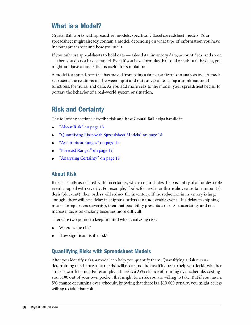
What is a Model?Crystal Ball works with spreadsheet models, specifically Excel spreadsheet models. Yourspreadsheet might already contain a model, depending on what type of information you havein your spreadsheet and how you use it.
If you only use spreadsheets to hold data — sales data, inventory data, account data, and so on— then you do not have a model. Even if you have formulas that total or subtotal the data, youmight not have a model that is useful for simulation.
A model is a spreadsheet that has moved from being a data organizer to an analysis tool. A modelrepresents the relationships between input and output variables using a combination offunctions, formulas, and data. As you add more cells to the model, your spreadsheet begins toportray the behavior of a real-world system or situation.
Risk and CertaintyThe following sections describe risk and how Crystal Ball helps handle it:
l “About Risk” on page 18
l “Quantifying Risks with Spreadsheet Models” on page 18
l “Assumption Ranges” on page 19
l “Forecast Ranges” on page 19
l “Analyzing Certainty” on page 19
About RiskRisk is usually associated with uncertainty, where risk includes the possibility of an undesirableevent coupled with severity. For example, if sales for next month are above a certain amount (adesirable event), then orders will reduce the inventory. If the reduction in inventory is largeenough, there will be a delay in shipping orders (an undesirable event). If a delay in shippingmeans losing orders (severity), then that possibility presents a risk. As uncertainty and riskincrease, decision-making becomes more difficult.
There are two points to keep in mind when analyzing risk:
l Where is the risk?
l How significant is the risk?
Quantifying Risks with Spreadsheet ModelsAfter you identify risks, a model can help you quantify them. Quantifying a risk meansdetermining the chances that the risk will occur and the cost if it does, to help you decide whethera risk is worth taking. For example, if there is a 25% chance of running over schedule, costingyou $100 out of your own pocket, that might be a risk you are willing to take. But if you have a5% chance of running over schedule, knowing that there is a $10,000 penalty, you might be lesswilling to take that risk.
18 Crystal Ball Overview
Finding the certainty of achieving a particular result is often the goal of model analysis. Riskanalysis takes a model and sees what effect changing different values has on the bottom line. Riskanalysis can:
l Help end "analysis paralysis" and contribute to better decision-making by quickly examiningall possible scenarios
l Identify which variables most affect the bottom-line forecast
l Expose the uncertainty in a model, leading to a better communication of risk
Assumption RangesFor each uncertain variable in a simulation, you can define the possible values with a probabilitydistribution. A simulation calculates numerous scenarios of a model by repeatedly picking valuesfrom the probability distribution for the uncertain variables and using those values for the cell.In Crystal Ball, distributions and associated scenario input values are called assumptions. Theyare entered and stored in assumption cells. For more information on assumptions andprobability distributions, see “About Assumptions and Probability Distributions” on page38.
Forecast RangesSince all those scenarios produce associated results, Crystal Ball also keeps track of the forecastsfor each scenario. These are important outputs of the model, such as totals, net profit, or grossexpenses. For each forecast, Crystal Ball remembers the cell value for all the trials (scenarios).After hundreds or thousands of trials, you can view sets of values, the statistics of the results(such as the mean forecast value), and the certainty of any particular value. Chapter 6 providesmore information about charts of forecast results and how to interpret them.
Analyzing CertaintyThe forecast results show the different result values for each forecast and also the probability ofobtaining any value. Crystal Ball normalizes these probabilities to calculate another importantnumber: the certainty.
The chance of any forecast value falling between –Infinity and +Infinity is always 100%.However, the chance — or certainty — of that same forecast being at least zero (which you mightwant to calculate to make sure that you make a profit) might be only 45%. For any range youdefine, Crystal Ball calculates the resulting certainty. This way, not only do you know that yourcompany has a chance to make a profit, but you can also quantify that chance by saying that thecompany has a 45% chance of making a profit on a venture (a venture you might, therefore,decide to skip).
How Crystal Ball Differs from Traditional Analysis ToolsWhen risk and uncertainty exist, traditional spreadsheet analysis tries to analyze this uncertaintyusing:
Model Building and Risk Analysis Overview 19
l “Point Estimates” on page 20
l “Range Estimates” on page 20
l “What-if Scenarios” on page 20
Point EstimatesPoint estimates are when you use what you think are the most likely values (technically referredto as the mode) for the uncertain variables. These estimates are the easiest, but can returnmisleading results. For example, try crossing a river with an average depth of three feet. Or, if ittakes you an average of 25 minutes to get to the airport, leave 25 minutes before your flight takesoff. You will miss your plane 50% of the time.
Range EstimatesRange estimates typically calculate three scenarios: the best case, the worst case, and the mostlikely case. These types of estimates can show you the range of outcomes, but not the probabilityof any of these outcomes.
What-if ScenariosWhat-if scenarios are usually based on range estimates, and are often constructed informally.What is the worst case for sales? What if sales are best case but expenses are the worst case? Whatif sales are average, but expenses are the best case? What if sales are average, expenses are average,but sales for the next month are flat?
These traditional methods have limitations:
l Changing only one spreadsheet cell at a time makes it virtually impossible to explore theentire range of possible outcomes.
l "What-if" analysis always results in single-point estimates that do not indicate the likelihoodof achieving any particular outcome. While single-point estimates might tell you what ispossible, they do not tell you what is probable.
This is where simulation with Crystal Ball comes in. Crystal Ball uses Monte Carlo simulationto generate a range of values for assumptions you define. These inputs feed into formulas definedin forecast cells.
You can use this process to explore ranges of outcomes, expressed as graphical forecasts. Youcan view and use forecast charts to estimate the probability, or certainty, of a particular outcome.
Monte Carlo Simulation and Crystal BallSpreadsheet risk analysis uses both a spreadsheet model and simulation to analyze the effect ofvarying inputs on outputs of the modeled system. One type of spreadsheet simulation is MonteCarlo simulation, which randomly generates values for uncertain variables over and over tosimulate a model.
20 Crystal Ball Overview
Monte Carlo simulation was named for Monte Carlo, Monaco, where the primary attractionsare casinos containing games of chance. Games of chance such as roulette wheels, dice, and slotmachines exhibit random behavior.
The random behavior in games of chance is similar to how Monte Carlo simulation selectsvariable values at random to simulate a model. When you roll a die, you know that either a 1,2, 3, 4, 5, or 6 will come up, but you do not know which for any particular trial. It is the samewith the variables that have a known range of values but an uncertain value for any particulartime or event (for example, interest rates, staffing needs, stock prices, inventory, phone calls perminute).
The following sections describe the benefits of Monte Carlo simulation and how it works inCrystal Ball:
l “Benefits of Monte Carlo Simulation” on page 21
l “How Crystal Ball Uses Monte Carlo Simulation” on page 21
Benefits of Monte Carlo SimulationCrystal Ball uses Monte Carlo simulation to overcome both of the spreadsheet limitationsencountered with traditional spreadsheet analysis (“How Crystal Ball Differs from TraditionalAnalysis Tools” on page 19):
l You can describe a range of possible values for each uncertain cell in your spreadsheet.Everything you know about each assumption is expressed all at once. For example, you candefine your business phone bill for future months as any value between $2500 and $3750,instead of using a single-point estimate of $3000. Crystal Ball then uses the defined range ina simulation.
l With Monte Carlo simulation, Crystal Ball displays results in a forecast chart that shows theentire range of possible outcomes and the likelihood of achieving each of them. In addition,Crystal Ball keeps track of the results of each scenario for you.
How Crystal Ball Uses Monte Carlo SimulationCrystal Ball implements Monte Carlo simulation in a repetitive three-step process. For each trialof a simulation, Crystal Ball repeats the following three steps:
1. For every assumption cell, Crystal Ball generates a random number according to theprobability distribution you defined and places it into the spreadsheet.
2. Crystal Ball recalculates the spreadsheet.
3. Crystal Ball then retrieves a value from every forecast cell and adds it to the chart in theforecast windows.
This is an iterative process that continues until either:
l The simulation reaches a stopping criterion
l You stop the simulation manually
Model Building and Risk Analysis Overview 21
The final forecast chart reflects the combined uncertainty of the assumption cells on the model’soutput. Keep in mind that Monte Carlo simulation can only approximate a real-world situation.When you build and simulate your own spreadsheet models, you need to carefully examine thenature of the problem and continually refine the models until they approximate your situationas closely as possible.
Crystal Ball Feature OverviewThe following sections introduce the main features of Crystal Ball:
l “Charts and Analysis Tools” on page 22
l “Other Crystal Ball Tools” on page 29
l “Process Capability Features” on page 31
l “Trend Analysis with Predictor” on page 31
l “Optimizing Decision Variable Values with OptQuest” on page 31
Charts and Analysis ToolsCrystal Ball offers several types of charts and reports, introduced in these sections:
l “Forecast Charts” on page 22
l “Overlay Charts” on page 23
l “Trend Charts” on page 24
l “Sensitivity Charts” on page 24
l “Scatter Charts” on page 25
l “Assumption Charts” on page 26
l “OptQuest Charts” on page 27
l “Reports” on page 27
l “Extracting and Pasting Data” on page 28
These graphical analysis tools are all accessed through the Analyze menu. They are discussed inChapter 6, “Analyzing Forecast Charts,” Chapter 7, “Analyzing Other Charts,”and Chapter 8,“Creating Reports and Extracting Data.”
Forecast ChartsForecast charts are the basic tool for Crystal Ball results analysis. They use frequency distributionsto show the number of values occurring in a given interval. The result is a range of valuesrepresenting possible and probable values for a given forecast formula based on inputassumption definitions. You can use forecast charts to evaluate the certainty of obtaining aparticular value or range of forecast values. For more information on forecast charts, seeChapter 6, “Analyzing Forecast Charts.”
22 Crystal Ball Overview
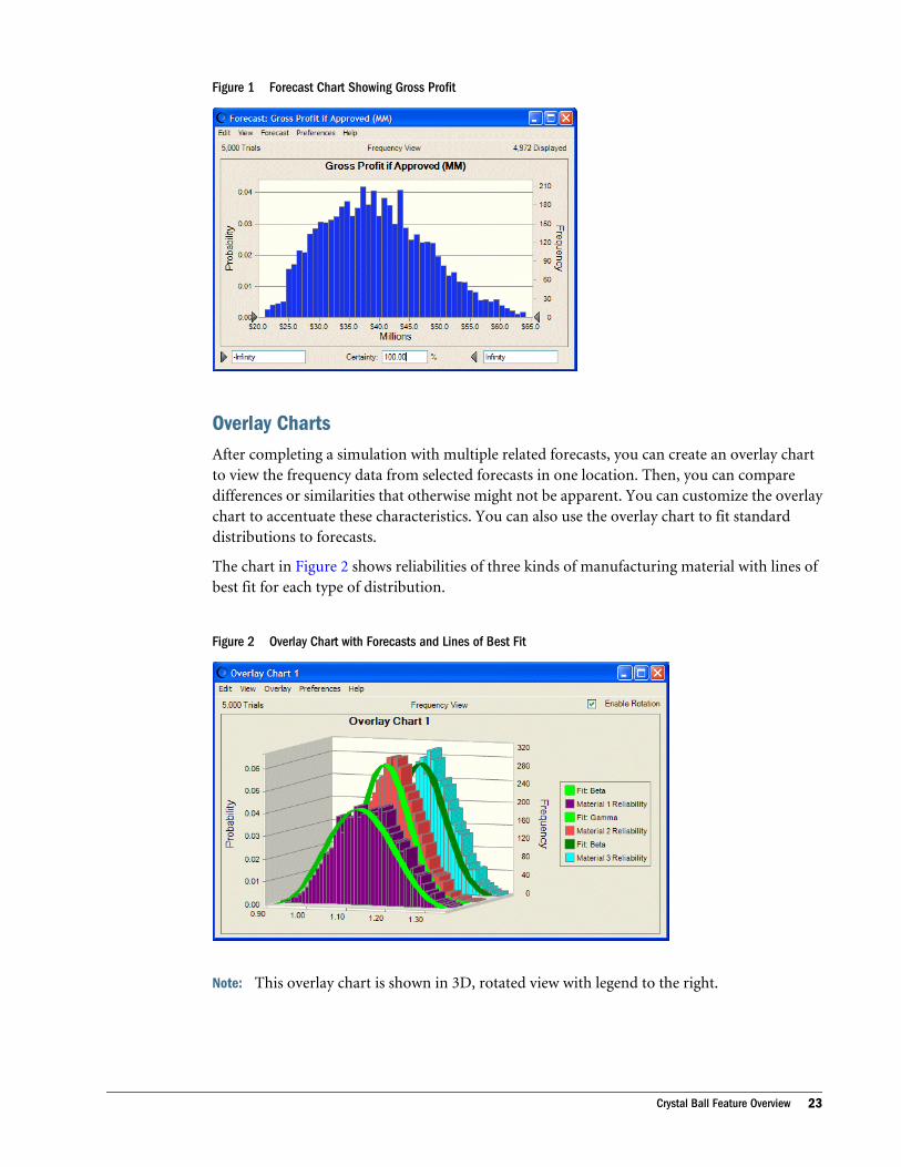
Figure 1 Forecast Chart Showing Gross Profit
Overlay ChartsAfter completing a simulation with multiple related forecasts, you can create an overlay chartto view the frequency data from selected forecasts in one location. Then, you can comparedifferences or similarities that otherwise might not be apparent. You can customize the overlaychart to accentuate these characteristics. You can also use the overlay chart to fit standarddistributions to forecasts.
The chart in Figure 2 shows reliabilities of three kinds of manufacturing material with lines ofbest fit for each type of distribution.
Figure 2 Overlay Chart with Forecasts and Lines of Best Fit
Note: This overlay chart is shown in 3D, rotated view with legend to the right.
Crystal Ball Feature Overview 23
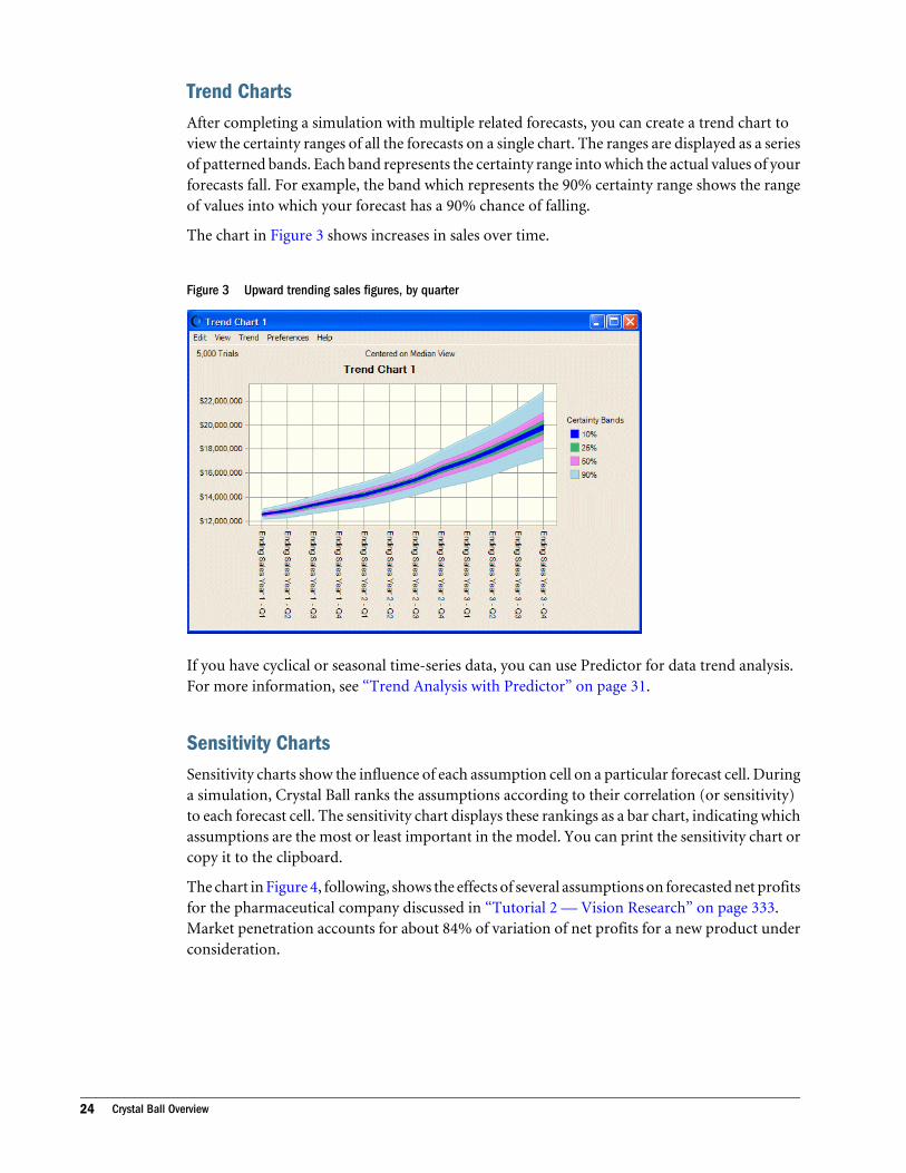
Trend ChartsAfter completing a simulation with multiple related forecasts, you can create a trend chart toview the certainty ranges of all the forecasts on a single chart. The ranges are displayed as a seriesof patterned bands. Each band represents the certainty range into which the actual values of yourforecasts fall. For example, the band which represents the 90% certainty range shows the rangeof values into which your forecast has a 90% chance of falling.
The chart in Figure 3 shows increases in sales over time.
Figure 3 Upward trending sales figures, by quarter
If you have cyclical or seasonal time-series data, you can use Predictor for data trend analysis.For more information, see “Trend Analysis with Predictor” on page 31.
Sensitivity ChartsSensitivity charts show the influence of each assumption cell on a particular forecast cell. Duringa simulation, Crystal Ball ranks the assumptions according to their correlation (or sensitivity)to each forecast cell. The sensitivity chart displays these rankings as a bar chart, indicating whichassumptions are the most or least important in the model. You can print the sensitivity chart orcopy it to the clipboard.
The chart in Figure 4, following, shows the effects of several assumptions on forecasted net profitsfor the pharmaceutical company discussed in “Tutorial 2 — Vision Research” on page 333.Market penetration accounts for about 84% of variation of net profits for a new product underconsideration.
24 Crystal Ball Overview

Figure 4 Effects of Assumptions on Net Profit
The Tornado Chart tool provides alternate ways to measure and chart sensitivity. For moreinformation, see “Tornado Chart” on page 30.
Scatter ChartsScatter charts show correlations, dependencies, and other relationships between pairs offorecasts and assumptions plotted against each other. You can plot scatter charts directly throughthe Analyze menu, or you can create a sensitivity chart and choose Sensitivity, then Open ScatterChart to create a chart showing how the assumptions with the greatest impact relate to the targetforecast.
In its basic form, a scatter chart (Figure 5) contains one or more plots of a target variable mappedagainst a set of secondary variables. Each plot is displayed as a cloud of points or symbols alignedin a grid within the scatter chart window. Optional correlation coefficients indicate the strengthof the relationship.
Crystal Ball Feature Overview 25
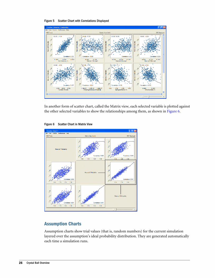
Figure 5 Scatter Chart with Correlations Displayed
In another form of scatter chart, called the Matrix view, each selected variable is plotted againstthe other selected variables to show the relationships among them, as shown in Figure 6.
Figure 6 Scatter Chart in Matrix View
Assumption ChartsAssumption charts show trial values (that is, random numbers) for the current simulationlayered over the assumption’s ideal probability distribution. They are generated automaticallyeach time a simulation runs.
26 Crystal Ball Overview
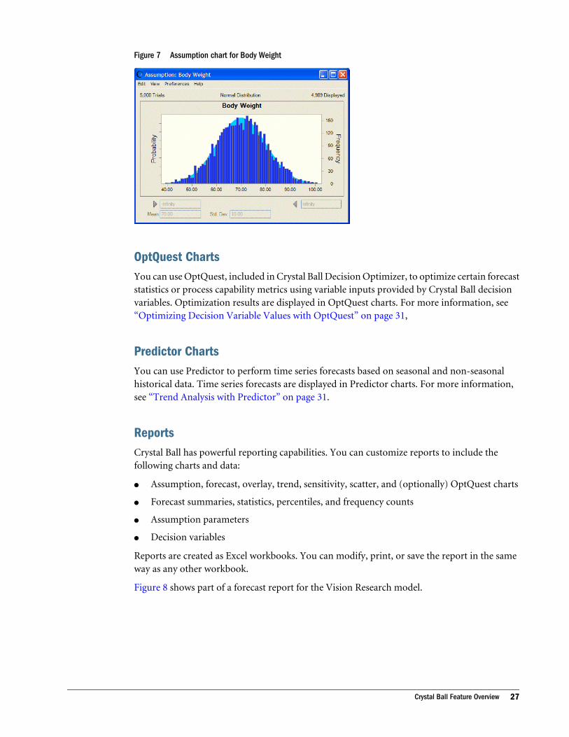
Figure 7 Assumption chart for Body Weight
OptQuest ChartsYou can use OptQuest, included in Crystal Ball Decision Optimizer, to optimize certain forecaststatistics or process capability metrics using variable inputs provided by Crystal Ball decisionvariables. Optimization results are displayed in OptQuest charts. For more information, see“Optimizing Decision Variable Values with OptQuest” on page 31,
Predictor ChartsYou can use Predictor to perform time series forecasts based on seasonal and non-seasonalhistorical data. Time series forecasts are displayed in Predictor charts. For more information,see “Trend Analysis with Predictor” on page 31.
ReportsCrystal Ball has powerful reporting capabilities. You can customize reports to include thefollowing charts and data:
l Assumption, forecast, overlay, trend, sensitivity, scatter, and (optionally) OptQuest charts
l Forecast summaries, statistics, percentiles, and frequency counts
l Assumption parameters
l Decision variables
Reports are created as Excel workbooks. You can modify, print, or save the report in the sameway as any other workbook.
Figure 8 shows part of a forecast report for the Vision Research model.
Crystal Ball Feature Overview 27
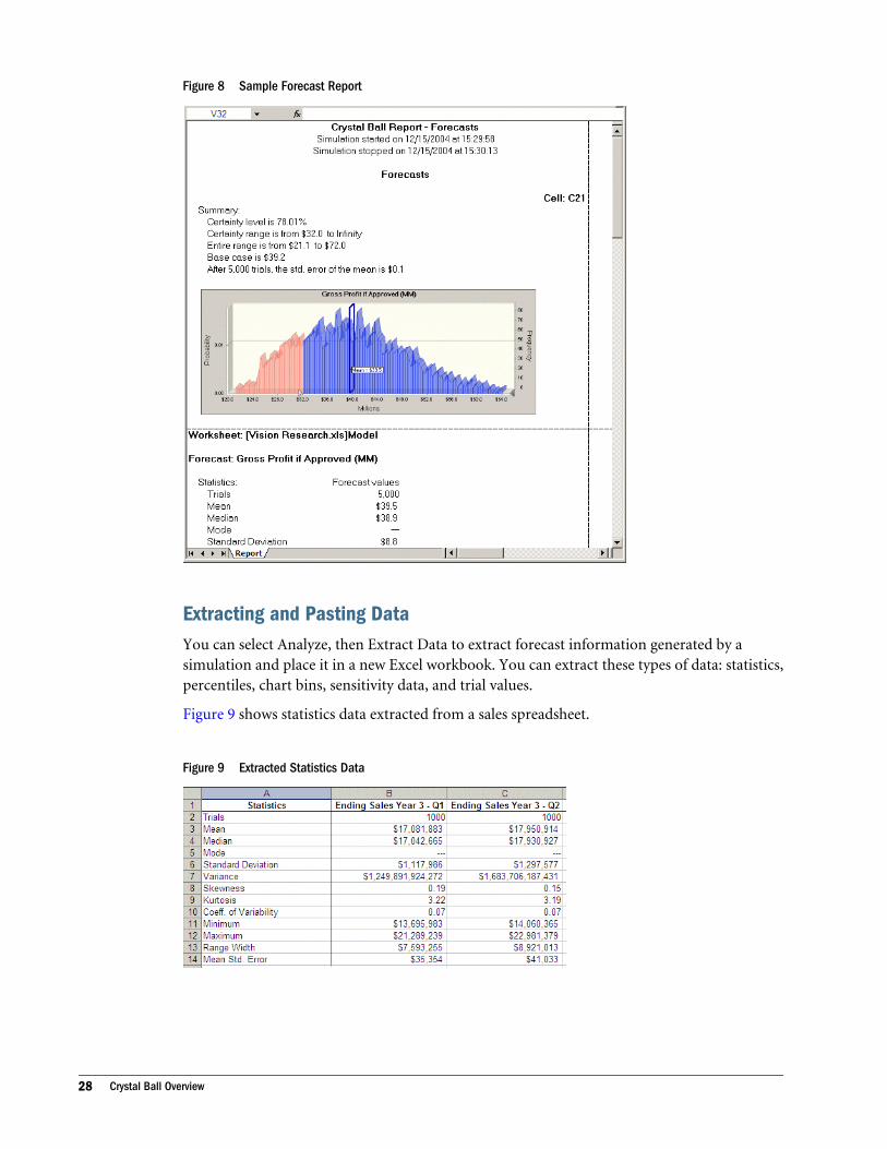
Figure 8 Sample Forecast Report
Extracting and Pasting DataYou can select Analyze, then Extract Data to extract forecast information generated by asimulation and place it in a new Excel workbook. You can extract these types of data: statistics,percentiles, chart bins, sensitivity data, and trial values.
Figure 9 shows statistics data extracted from a sales spreadsheet.
Figure 9 Extracted Statistics Data
28 Crystal Ball Overview
Other Crystal Ball ToolsThe Run menu offers a variety of special tools for analyzing your data and displaying results inmore detail. Select Run, then More Tools to choose from tools discussed in the following sections(in Microsoft Excel 2007, select More Tools in the Tools group of the Crystal Ball ribbon):
l “Batch Fit” on page 29
l “Bootstrap” on page 29
l “Correlation Matrix” on page 29
l “Data Analysis” on page 30
l “Decision Table” on page 30
l “Scenario Analysis” on page 30
l “Tornado Chart” on page 30
l “2D Simulation” on page 30
l “Integration Tools” on page 30
l “Compare Run Modes” on page 31
All of these except the integration tools are discussed in Chapter 9, “Crystal Ball Tools.”. Theintegraton tools are only available in Crystal Ball EPM and are described in the Oracle CrystalBall Enterprise Performance Management Integration Guide.
Additional tools, Predictor and OptQuest, may also appear on the Run menu (or the Tools groupiin Microsoft Excel 2007) in certain editions of Crystal Ball. For a description of these features,see “Trend Analysis with Predictor” on page 31 and “Optimizing Decision Variable Valueswith OptQuest” on page 31.
Batch FitThe Batch Fit tool fits probability distributions to multiple data series. It helps create assumptionswhen you have historical data for several variables. Inputs are rows or columns of data. Outputsinclude fitted assumptions (probability distributions), tables of goodness-of-fit statistics andcorrelation coefficients calculated from the data series.
BootstrapThe Bootstrap too estimates the reliability or accuracy of statistics or percentiles for forecasts orother sample data. This tool doesn’t assume that the statistics or percentiles are normallydistributed. The main input is the forecast to be analyzed. Outputs are a forecast chart of thedistributions for each statistic or percentile.
Correlation MatrixThe Correlation Matrix tool defines a matrix of correlations between assumptions to moreaccurately model the interdependencies between variables. Inputs are the assumptions tocorrelate. The output is a correlation matrix, loaded into the model.
Crystal Ball Feature Overview 29
Data AnalysisThe Data Analysis tool imports data directly into Crystal Ball forecasts for analysis in CrystalBall.
Decision TableDecision variables are values you can control, such as such as how much to charge for a productor how many wells to drill. The Decision Table tool runs multiple simulations to test differentvalues for one or two decision variables. Inputs are the decision variables to test. The output isa table of results you can analyze further using forecast, trend, or overlay charts.
If you want to optimize decision variable values to reach a specific objective and you haveOptQuest, you can use it to find solutions. For more information, see “Optimizing DecisionVariable Values with OptQuest” on page 31.
Scenario AnalysisThe Scenario Analysis tool runs a simulation and then matches all of the resulting values of atarget forecast with the corresponding assumption values. Then, you can see which combinationof assumption values gives a particular result. The input is the forecast to be analyzed. The outputis a table of all the forecast values matched with the corresponding value of each assumption.
Tornado ChartThe Tornado Chart tool measures the input of each model variable one at a time, independently,on a target forecast. The inputs are the target forecast and the assumptions, decision variables,and precedent cells to test against. The output is a tornado chart, which shows the sensitivity ofthe variables using range bars, or a spider chart, which shows the sensitivity of the variables usingsloping lines.
2D SimulationThe 2D Simulation tool helps determine how much of the variation within a model is causedby uncertainty and how much by true variability. The inputs are the target forecast and theassumptions to analyze. The output is a table which includes the forecast means, the uncertaintyassumption values, and the statistics, including percentiles, of the forecast distribution for eachsimulation. Results are also graphed on an overlay chart and a trend chart.
Integration ToolsThe optional integration tools link Crystal Ball EPM with Oracle Hyperion Strategic Finance,Fusion Edition and other Enterprise Performance Management applications using the StrategicFinance Setup wizard and Oracle Hyperion Smart View for Office, Fusion Edition. The StrategicFinance tool creates a workbook of Strategic Finance information that can then be analyzed withCrystal Ball. The Enterprise Performance Management tool connects to Oracle EnterprisePerformance Management applications such as Oracle Essbase using Smart View so you can run
30 Crystal Ball Overview
Crystal Ball simulations on data in the underlying database. The integration tools are onlyavailable if you have Strategic Finance and Crystal Ball EPM. They are described in the StrategicFinance Integration Guide and a help file that is available after you start the Strategic FinanceSetup wizard.
Compare Run ModesIf you have Crystal Ball Decision Optimizer including the Extreme Speed feature, you can usethe Compare Run Modes tool to compare simulation run time in Normal and Extreme speed.For more information about this tool, see Appendix C, “Using the Extreme Speed Feature”.
Process Capability FeaturesIf you use Six Sigma or other quality methodologies, Crystal Ball’s process capability featurescan help you improve quality in your organization. For a brief description of these features andhow to use them, see Appendix E, “Using the Process Capability Features.”
Trend Analysis with PredictorYou can use Predictor to project trends based on time-series data, such as seasonal trends.
For example, you can look at home heating fuel sales for previous years and estimate sales forthe current year. You can also run regression analysis on related time-series data.
For more information about Predictor, see the Oracle Crystal Ball Predictor User's Guide.
Optimizing Decision Variable Values with OptQuestDecision variables are variables you can control, such as product pricing or investment levels.If you have OptQuest, an optional feature available in Crystal Ball Decision Optimizer, you canuse it to find the best values for the decision variables to obtain the desired outcomes.
For example, you can find the optimal investment mix that maximizes the probability of aportfolio’s return being above a certain threshold.
For more information about OptQuest, see the Oracle Crystal Ball Decision Optimizer OptQuestUser's Guide.
Steps for Using Crystal BallFollow these general steps to create and interpret simulations with Crystal Ball. The remainingchapters provide detailed instructions:
1. Create a spreadsheet model in Microsoft Excel format with data and formula cells thatrepresent the situation to analyze.
Steps for Using Crystal Ball 31
“What is a Model?” on page 18 discusses spreadsheet models. Also see the references in theBibliography.
2. Start Crystal Ball.
If you have not set up Crystal Ball to load automatically with Microsoft Excel, start CrystalBall as described in “Starting and Closing Crystal Ball” on page 32.
3. Load your spreadsheet model.
4. Using Crystal Ball, define assumption cells and forecast cells. If appropriate for yoursituation, you can also define decision variable cells.
For more information, see “Entering Assumptions” on page 38 and continue on withChapter 4.
5. Set run preferences for your simulation, as described in “Setting Run Preferences” on page76.
6. Run the simulation, following the instructions in “Starting Simulations” on page 81.
7. Analyze your results. See “Understanding and Using Forecast Charts” on page 95 forsuggestions.
8. Consider using Predictor or OptQuest, if available, for further analysis.
9. Take advantage of the many resources available to help you get the most out of Crystal Ball.
Resources for Learning Crystal BallIf you are new to Crystal Ball, Appendix D offers tutorials to quickly introduce Crystal Ball’sfeatures and workflow. Consider completing the tutorials before you continue on with the moredetailed instructions that follow.
For information on support, training, and referral services, see the Crystal BallWeb site at:
http://www.oracle.com/crystalball
Starting and Closing Crystal BallYou can start Crystal Ball manually or you can set up Crystal Ball to start automatically wheneveryou start Excel.
Starting Crystal Ball Manually
ä To start Crystal Ball manually, in Windows, choose Start, then All Programs, then Oracle CrystalBall, then Crystal Ball.
Excel opens with the Crystal Ball menus and toolbar. If Excel is already running when you givethis command, Crystal Ball opens a new instance of Excel.
32 Crystal Ball Overview
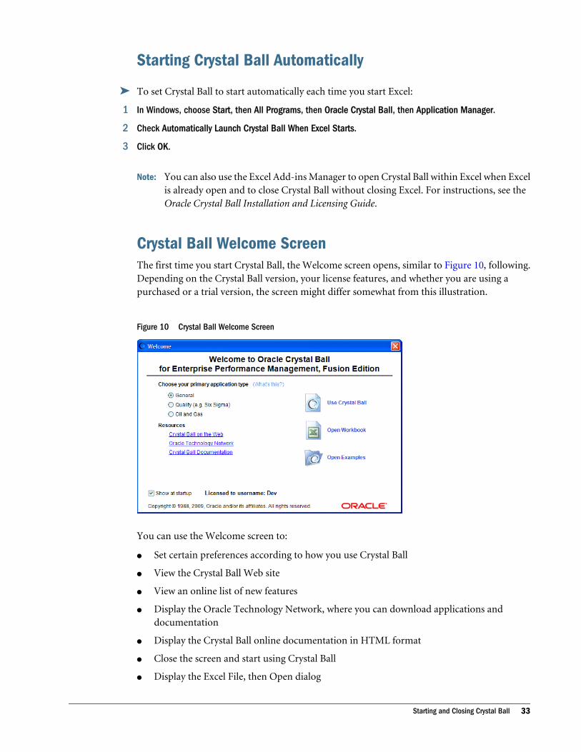
Starting Crystal Ball Automatically
ä To set Crystal Ball to start automatically each time you start Excel:
1 In Windows, choose Start, then All Programs, then Oracle Crystal Ball, then Application Manager.
2 Check Automatically Launch Crystal Ball When Excel Starts.
3 Click OK.
Note: You can also use the Excel Add-ins Manager to open Crystal Ball within Excel when Excelis already open and to close Crystal Ball without closing Excel. For instructions, see theOracle Crystal Ball Installation and Licensing Guide.
Crystal Ball Welcome ScreenThe first time you start Crystal Ball, the Welcome screen opens, similar to Figure 10, following.Depending on the Crystal Ball version, your license features, and whether you are using apurchased or a trial version, the screen might differ somewhat from this illustration.
Figure 10 Crystal Ball Welcome Screen
You can use the Welcome screen to:
l Set certain preferences according to how you use Crystal Ball
l View the Crystal Ball Web site
l View an online list of new features
l Display the Oracle Technology Network, where you can download applications anddocumentation
l Display the Crystal Ball online documentation in HTML format
l Close the screen and start using Crystal Ball
l Display the Excel File, then Open dialog
Starting and Closing Crystal Ball 33
l Display the Oracle Crystal Ball Examples Guide
l Purchase Crystal Ball, if you are using a time-limited trial version
For an explanation of the “primary application type” settings, click the What Is This? hyperlink.
Closing Crystal Ball
ä To close Crystal Ball, use one of the following options::
l Right-click the Crystal Ball icon, , in the Windows taskbar and choose Close,or
l Close Excel.
If you want, you can choose Run, then Reset Simulation to reset the model and then choose File,then Save to save it before you close Crystal Ball.
Crystal Ball Menus and ToolbarThe following sections describe the main elements of the Crystal Ball user interface:
l “The Crystal Ball Menus” on page 34
l “The Crystal Ball Toolbar” on page 35
The Crystal Ball MenusWhen you load Crystal Ball with Microsoft Excel, some new menus are displayed in the Excelmenubar:
l Define — contains commands that define and select assumption, decision variable, andforecast cells; perform Crystal Ballcopy data, paste data, and clear data operations; and setcell preferences.
l Run — contains commands that start, stop, reset, and single-step through simulations;freeze variables; launch the Crystal Balltools and Predictor as well as OptQuest, if available;and set run preferences.
l Analyze — contains commands that create a variety of charts and reports, extract data, andsave or restore results.
For specific information about commands, see Appendix B, “Accessibility.”
Note: If you are using Crystal Ball in Excel 2007, you will see a single Crystal Ball menu and thena ribbon instead of a toolbar. For more information about using Crystal Ball with Office2007, see Appendix B.
34 Crystal Ball Overview
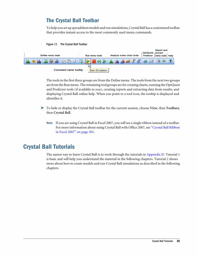
The Crystal Ball ToolbarTo help you set up spreadsheet models and run simulations, Crystal Ball has a customized toolbarthat provides instant access to the most commonly used menu commands.
Figure 11 The Crystal Ball Toolbar
The tools in the first three groups are from the Define menu. The tools from the next two groupsare from the Run menu. The remaining tool groups are for creating charts, running the OptQuestand Predictor tools (if available to you), creating reports and extracting data from results, anddisplaying Crystal Ball online help. When you point to a tool icon, the tooltip is displayed andidentifies it.
ä To hide or display the Crystal Ball toolbar for the current session, choose View, then Toolbars,then Crystal Ball.
Note: If you are using Crystal Ball in Excel 2007, you will see a single ribbon instead of a toolbar.For more information about using Crystal Ball with Office 2007, see “Crystal Ball Ribbonin Excel 2007” on page 301.
Crystal Ball TutorialsThe easiest way to learn Crystal Ball is to work through the tutorials in Appendix D. Tutorial 1is basic and will help you understand the material in the following chapters. Tutorial 2 showsmore about how to create models and run Crystal Ball simulations as described in the followingchapters.
Crystal Ball Tutorials 35

36 Crystal Ball Overview
3Defining Model Assumptions
In This Chapter
Introduction... . . . . . . . . . . . . . . . . . . . . . . . . . . . . . . . . . . . . . . . . . . . . . . . . . . . . . . . . . . . . . . . . . . . . . . . . . . . . . . . . . . . . . . . . . . . . . . . . . . . . . . . . . . . . . . . . . . . . . .37
Types of Data Cells .. . . . . . . . . . . . . . . . . . . . . . . . . . . . . . . . . . . . . . . . . . . . . . . . . . . . . . . . . . . . . . . . . . . . . . . . . . . . . . . . . . . . . . . . . . . . . . . . . . . . . . . . . . . . . . .37
About Assumptions and Probability Distributions... . . . . . . . . . . . . . . . . . . . . . . . . . . . . . . . . . . . . . . . . . . . . . . . . . . . . . . . . . . . . . . . . . . . . . . . . . . . .38
Defining Assumptions ... . . . . . . . . . . . . . . . . . . . . . . . . . . . . . . . . . . . . . . . . . . . . . . . . . . . . . . . . . . . . . . . . . . . . . . . . . . . . . . . . . . . . . . . . . . . . . . . . . . . . . . . . . .38
Entering Assumptions ... . . . . . . . . . . . . . . . . . . . . . . . . . . . . . . . . . . . . . . . . . . . . . . . . . . . . . . . . . . . . . . . . . . . . . . . . . . . . . . . . . . . . . . . . . . . . . . . . . . . . . . . . . .38
Additional Assumption Features... . . . . . . . . . . . . . . . . . . . . . . . . . . . . . . . . . . . . . . . . . . . . . . . . . . . . . . . . . . . . . . . . . . . . . . . . . . . . . . . . . . . . . . . . . . . . . . .41
Using the Crystal Ball Distribution Gallery .. . . . . . . . . . . . . . . . . . . . . . . . . . . . . . . . . . . . . . . . . . . . . . . . . . . . . . . . . . . . . . . . . . . . . . . . . . . . . . . . . . . . . .51
IntroductionThis chapter provides step-by-step instructions for setting up assumption cells in Crystal Ballmodels so simulations can be run against them. This chapter also describes all the ways you canuse the Distribution Gallery to organize your favorite distributions and define categories ofdistributions to share with others. The next chapter describes how to define decision variableand forecast cells and to cut, copy, and paste data.
If you are a new user, you should start by working through the tutorials in Appendix D, andthen read this chapter. After you complete this chapter and Chapter 4, read Chapter 5 forinformation on setting preferences and running simulations.
Types of Data CellsCrystal Ball uses three types of data cells as inputs and outputs:
l Assumption cells are input cells that contain values that you are unsure of: the uncertainindependent variables in the problem you are trying to solve. The assumption cells mustcontain simple numeric values, not formulas or text.
l Decision variable cells are input cells that contain values that are within your control tochange. The decision variable cells must contain simple numeric values, not formulas ortext. These are used by some of the Crystal Ball tools and by OptQuest.
l Forecast cells (dependent variables) are output cells that contain formulas that refer to oneor more assumption and decision variable cells. The forecast cells combine the values in theassumption, decision variable, and other cells to calculate a result. A forecast cell, forexample, might contain the formula =C17*C20*C21.
Introduction 37
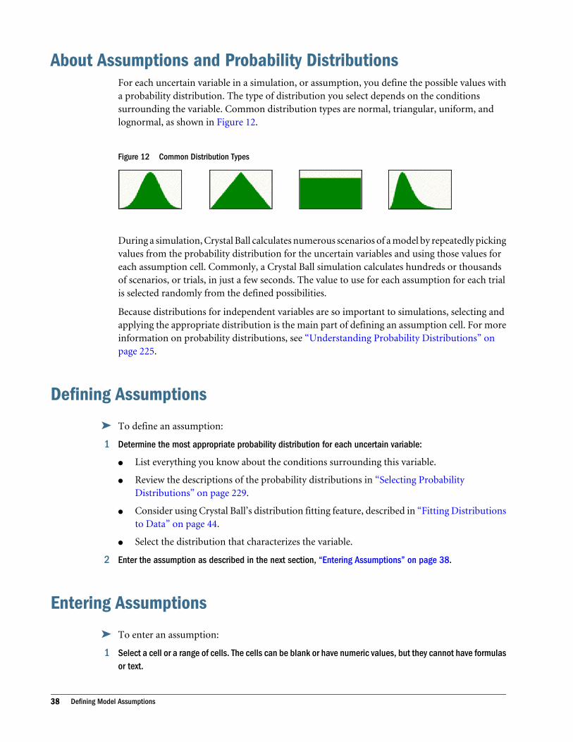
About Assumptions and Probability DistributionsFor each uncertain variable in a simulation, or assumption, you define the possible values witha probability distribution. The type of distribution you select depends on the conditionssurrounding the variable. Common distribution types are normal, triangular, uniform, andlognormal, as shown in Figure 12.
Figure 12 Common Distribution Types
During a simulation, Crystal Ball calculates numerous scenarios of a model by repeatedly pickingvalues from the probability distribution for the uncertain variables and using those values foreach assumption cell. Commonly, a Crystal Ball simulation calculates hundreds or thousandsof scenarios, or trials, in just a few seconds. The value to use for each assumption for each trialis selected randomly from the defined possibilities.
Because distributions for independent variables are so important to simulations, selecting andapplying the appropriate distribution is the main part of defining an assumption cell. For moreinformation on probability distributions, see “Understanding Probability Distributions” onpage 225.
Defining Assumptions
ä To define an assumption:
1 Determine the most appropriate probability distribution for each uncertain variable:
l List everything you know about the conditions surrounding this variable.
l Review the descriptions of the probability distributions in “Selecting ProbabilityDistributions” on page 229.
l Consider using Crystal Ball’s distribution fitting feature, described in “Fitting Distributionsto Data” on page 44.
l Select the distribution that characterizes the variable.
2 Enter the assumption as described in the next section, “Entering Assumptions” on page 38.
Entering Assumptions
ä To enter an assumption:
1 Select a cell or a range of cells. The cells can be blank or have numeric values, but they cannot have formulasor text.
38 Defining Model Assumptions

2 Choose Define, then Define Assumption, .
(In Excel 2007, click the upper half of the Define Assumption icon.)
For each selected cell or cells in the selected range, Crystal Ball displays the Distribution Gallerydialog (Figure 13).
Figure 13 The Distribution Gallery with Basic category Selected
3 In the Distribution Gallery, select the distribution you want from the gallery. The Basic category containsseveral frequently used distributions. Click All to view all distributions shipped with Crystal Ball. For details,see “Using the Crystal Ball Distribution Gallery” on page 51.
Alternately, click the Fit button to fit a distribution to historical data, as described in “FittingDistributions to Data” on page 44.
For more information on the Distribution Gallery, see “Distribution Gallery Window” on page51.
4 When the Define Assumption dialog opens (Figure 14), type in a title and the parameters for the distribution.The parameters can be either numeric values or cell references.
Entering Assumptions 39
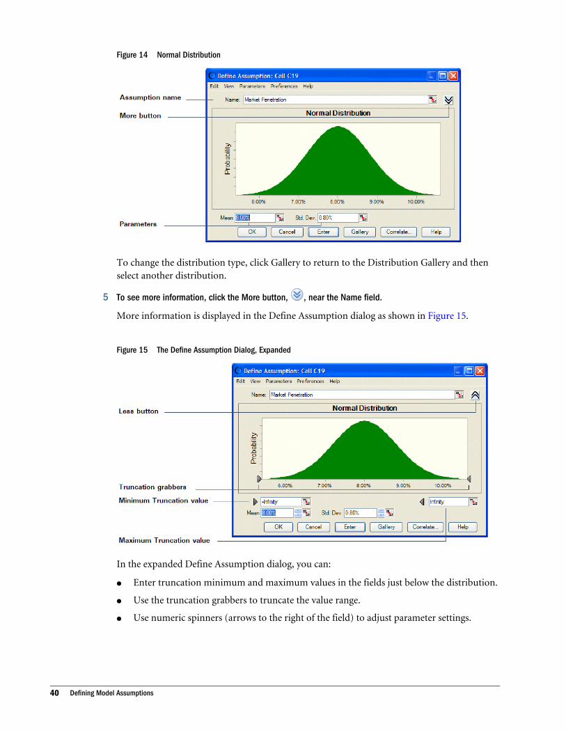
Figure 14 Normal Distribution
To change the distribution type, click Gallery to return to the Distribution Gallery and thenselect another distribution.
5 To see more information, click the More button, , near the Name field.
More information is displayed in the Define Assumption dialog as shown in Figure 15.
Figure 15 The Define Assumption Dialog, Expanded
In the expanded Define Assumption dialog, you can:
l Enter truncation minimum and maximum values in the fields just below the distribution.
l Use the truncation grabbers to truncate the value range.
l Use numeric spinners (arrows to the right of the field) to adjust parameter settings.
40 Defining Model Assumptions
l Click the Less button, , to hide the minimum and maximum value fields and truncationgrabbers. (For more information about truncating distributions, see “TruncatingDistributions” on page 280.)
You can perform the following activities in both the standard and expanded Define Assumptiondialog:
l Click the Gallery button to display the Distribution Gallery window and choose anotherdistribution.
l Click the Correlate button to define correlations as described in “Specifying CorrelationsBetween Assumptions” on page 47.
l Choose Edit, then Add in the menubar to add the currently defined assumption distributionto the Favorites category or a user-defined category in the Distribution Gallery.
l Use other menu commands to copy the chart, paste it into Excel or another application,print data, change the view, use alternate parameters, set assumption and chart preferences,and display help as described in “Additional Assumption Features” on page 41.
6 When you have finished entering parameters to define the assumption, click Enter.
The distribution changes to reflect the values you entered. If you click OK instead of Enter,Crystal Ball accepts the parameters and closes the dialog.
7 Click OK.
If you selected a range of cells, repeat these steps to define the assumption for each cell.
Additional Assumption FeaturesAs you enter assumption parameters, you can use cell references and alternate parameters. Ifyou have historical data available, you can use Crystal Ball’s distribution fitting feature to helpsimplify the process of selecting a probability distribution. You can also specify correlationsbetween assumptions or freeze assumptions to exclude them from a simulation.
The following sections discuss advanced features that help you refine assumption definitionsand use assumptions more effectively:
l “ Entering Cell References and Formulas” on page 42 below
l “Alternate Parameter Sets” on page 43
l “Fitting Distributions to Data” on page 44
l “Specifying Correlations Between Assumptions” on page 47
l “Setting Assumption Preferences” on page 50
l “Freezing Crystal Ball Data Cells” on page 80
Additional Assumption Features 41
Entering Cell References and FormulasIn addition to numeric values, you can enter a reference to a specific cell in a parameter field.Cell references must be preceded by an equal sign (=). Cell references can be either absolute orrelative. You can also enter formulas and range names.
If necessary, you can press F4 to change references from relative to absolute or back to relative.This also applies to cell references in fields other than assumption parameters.
Note: All cell references in parameters are treated like absolute references when cutting andpasting Crystal Ball data. Crystal Ball always stores the cell reference in A1 format even ifthe Excel preference is set to R1C1 format. The global R1C1 format preference is notaffected by running Crystal Ball, but the name ranges are, in fact, changed to A1 formatsince that is the way Crystal Ball stores them.
ä To show cell references instead of current values when you enter them in parameter fields, chooseParameters, then Show Cell References in the Define Assumption dialog.
The following topics contain details about cell references, range names, and formulas:
l “Dynamic vs. Static Cell References” on page 42
l “Relative References” on page 42
l “Absolute References” on page 43
l “Range Names” on page 43
l “Formulas” on page 43
Dynamic vs. Static Cell ReferencesCell references in assumption parameters are dynamic and are updated each time the workbookis recalculated. Dynamic cell referencing gives you more flexibility in setting up models becauseyou can change an assumption’s distribution during a simulation.
Other types of cell references are static, such as the assumption name field and correlationcoefficients. These cell references are calculated once at the beginning of a simulation.
Relative ReferencesRelative references describe the position of a cell relative to the cell containing the assumption.For example, suppose an assumption in cell C6 refers to cell C5. If the assumption in C6 is copiedto cell C9, the relative reference to C5 will then refer to the value in cell C8. With relativereferences, you can easily set up a whole row or column of assumptions, each having similardistributions but slightly different parameters, by performing just a few steps. An absolutereference, on the other hand, always refers back to the originally referenced cell, in this case C5.
42 Defining Model Assumptions
Absolute ReferencesTo indicate an absolute reference, use a dollar sign ($) before the row and the column. Forexample, to copy the exact contents of cell C5 into an assumption parameter field, enter the cellreference =$C$5. This causes the value in cell C5 to be used in the assumption cell parameterfield. Later, if you decide to copy and paste this assumption in the worksheet, the cell referencesin the parameter field will refer to the contents of cell C5.
Range NamesYou can also enter cell references in the form of range names, such as =cellname. Then, thereferenced cell can be located anywhere within a worksheet as long as its name does not change.
FormulasYou can enter Excel formulas to calculate parameter values as long as the formula resolves tothe type of data acceptable for that parameter. For example, if a formula returns a string, it wouldnot be acceptable in a parameter that requires a numeric value, such as Minimum or Maximum.
Alternate Parameter SetsFor all the continuous probability distributions except uniform, you can use percentiles forparameters when defining a distribution. This option gives you added flexibility to set upassumptions when only percentile information is available or when specific attributes (such asthe mean and standard deviation) of the variable in your model are unknown.
For example, if you are defining a triangular distribution, but are unsure of the absoluteminimum and maximum values of the variable, you can instead define the distribution usingthe 10th and 90th percentiles along with the likeliest value. This gives you a distribution that has80%, or four-fifths of the values, occurring between the two specified percentiles.
To change the parameter sets for the continuous distributions, use the Parameters menu in themenubar of the Define Assumption dialog. The currently selected parameter set has a checkmark next to it. If you choose Custom in the Parameters menu, you can replace any or all of thestandard parameters with any percentile.
To select a parameter set to use as the default when defining new assumptions of this type, chooseSet Default from the Parameters menu.
Several special parameter sets are available with the lognormal distribution, including geometricand logarithmic sets. For more information, see the "Equations and Methods" chapter in theonline Oracle Crystal Ball Statistical Guide.
Note: Alternate parameters cannot always be used with highly skewed distributions andextremely large or small parameter values.
Additional Assumption Features 43
Fitting Distributions to DataIf you have historical data available, Crystal Ball’s distribution fitting feature can substantiallysimplify the process of selecting a probability distribution. Not only is the process simplified,but the resulting distribution more accurately reflects the nature of your data than if the shapeand parameters of the distribution were estimated.
Distribution fitting automatically matches historical data against probability distributions. Amathematical fit determines the set of parameters for each distribution that best describe thecharacteristics of the data. Then, the closeness of each fit is judged using one of several standardgoodness-of-fit tests. The highest ranking fit is chosen to represent the data. You can choosefrom among all distributions supported by Crystal Ballexcept the yes-no distribution.
Using Distribution Fitting
ä To use distribution fitting:
1 Select the cell where you want to create an assumption.
It can be blank or contain a simple value, not a formula.
2 Choose Define, then Define Assumption, .
(In Excel 2007, click the upper half of the Define Assumption icon.)
3 In the Distribution Gallery, click Fit to select the source of the fitted data.
The Fit Distribution dialog opens.
4 Choose a data location.
l If the historical data is in a worksheet in the active workbook, choose Range, and then enterthe data’s cell range. If the range has a name, you can enter the name, preceded by an = sign.
l If the historical data is in a separate text file, click Text File, and then either enter the pathand name of the file or click Browse to search for the file. If you want, you can check Columnand enter the number of columns in the text file.
When you use a file as your source of data, each data value in the file must be separated byeither a comma, a tab character, a space character, or a list separator defined in Windows’Regional and Language Options panel. If actual values in the file contain commas or thedesignated list separator, those values must be enclosed in quotes. Allowable formats forvalues are identical to those allowed within the assumption parameter dialog, including date,time, currency, and numbers.
5 Specify which distributions are to be fitted:
l AutoSelect performs a basic analysis of the data to choose a distribution fitting option andranking method. If the data includes only integers, fitting to all discrete distributions (withthe exception of Yes-No) is completed using the Chi-square ranking statistic choice.
l All Continuous fits the data to all of the built-in continuous distributions (thesedistributions are displayed as solid shapes on the Distribution Gallery).
44 Defining Model Assumptions
l All Discrete fits to all discrete distributions except yes-no and uses the Chi-square rankingstatistic.
l Choose displays another dialog where you can select a subset of the distributions to includein the fitting.
l The final setting selects the distribution that was highlighted on the Distribution Gallerywhen you clicked the Fit button.
If you try to fit negative data to a distribution that can only accept positive data, thatdistribution will not be fitted to the data.
6 Specify how the distributions should be ranked.
In ranking the distributions, you can use any one of three standard goodness-of-fit tests:
l Anderson-Darling. This method closely resembles the Kolmogorov-Smirnov method,except that it weights the differences between the two distributions at their tails greater thanat their mid-ranges. This weighting of the tails helps to correct the Kolmogorov-Smirnovmethod’s tendency to over-emphasize discrepancies in the central region.
l Chi-Square. This test is the oldest and most common of the goodness-of-fit tests. It gaugesthe general accuracy of the fit. The test breaks down the distribution into areas of equalprobability and compares the data points within each area to the number of expected datapoints. The chi-square test in Crystal Ball does not use the associated p-value the way otherstatistical tests (e.g., t or F) do.
l Kolmogorov-Smirnov. The result of this test is essentially the largest vertical distancebetween the two cumulative distributions.
The first setting, AutoSelect,, selects the ranking statistic automatically based on severalfactors. If all data values are integers, Chi-Square is selected.
7 If you know your data corresponds to certain shape, location, or other special parameter values for somedistributions, you can choose to lock parameters to those values.
Check Lock Parameters and enter appropriate values in the Lock Parameters dialog. For details,see “Locking Parameters When Fitting Distributions” on page 47.
8 By default, only values for the selected ranking statistic are displayed in the Comparison Chart dialog. Toshow values for all three statistics, check Show All Goodness-of-fit Statistics at the bottom of the FitDistribution dialog.
9 Click OK.
The Comparison Chart opens.
Confirming the Fitted DistributionWhen the Comparison Chart opens (Figure 16), the fitted distributions are displayed in theComparison Chart dialog, starting with the highest-ranked distribution (best fit) down throughto the lowest (worst fit).
Additional Assumption Features 45
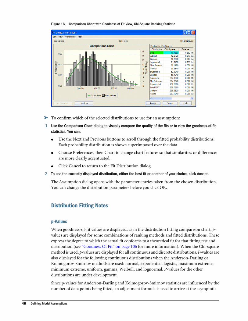
Figure 16 Comparison Chart with Goodness of Fit View, Chi-Square Ranking Statistic
ä To confirm which of the selected distributions to use for an assumption:
1 Use the Comparison Chart dialog to visually compare the quality of the fits or to view the goodness-of-fitstatistics. You can:
l Use the Next and Previous buttons to scroll through the fitted probability distributions.Each probability distribution is shown superimposed over the data.
l Choose Preferences, then Chart to change chart features so that similarities or differencesare more clearly accentuated.
l Click Cancel to return to the Fit Distribution dialog.
2 To use the currently displayed distribution, either the best fit or another of your choice, click Accept.
The Assumption dialog opens with the parameter entries taken from the chosen distribution.You can change the distribution parameters before you click OK.
Distribution Fitting Notes
p-Values
When goodness-of-fit values are displayed, as in the distribution fitting comparison chart, p-values are displayed for some combinations of ranking methods and fitted distributions. Theseexpress the degree to which the actual fit conforms to a theoretical fit for that fitting test anddistribution (see “Goodness Of Fit” on page 106 for more information). When the Chi-squaremethod is used, p-values are displayed for all continuous and discrete distributions. P-values arealso displayed for the following continuous distributions when the Anderson-Darling orKolmogorov-Smirnov methods are used: normal, exponential, logistic, maximum extreme,minimum extreme, uniform, gamma, Weibull, and lognormal. P-values for the otherdistributions are under development.
Since p-values for Anderson-Darling and Kolmogorov-Smirnov statistics are influenced by thenumber of data points being fitted, an adjustment formula is used to arrive at the asymptotic
46 Defining Model Assumptions
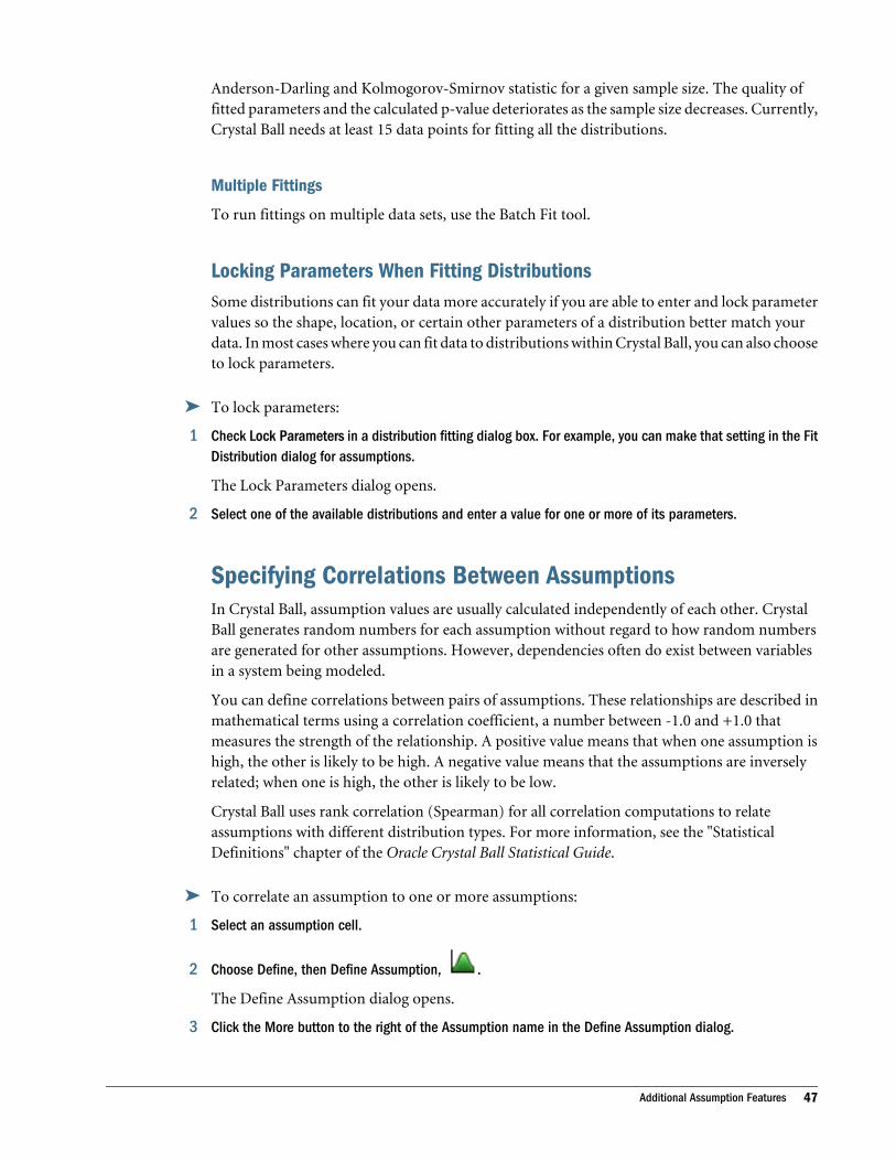
Anderson-Darling and Kolmogorov-Smirnov statistic for a given sample size. The quality offitted parameters and the calculated p-value deteriorates as the sample size decreases. Currently,Crystal Ball needs at least 15 data points for fitting all the distributions.
Multiple Fittings
To run fittings on multiple data sets, use the Batch Fit tool.
Locking Parameters When Fitting DistributionsSome distributions can fit your data more accurately if you are able to enter and lock parametervalues so the shape, location, or certain other parameters of a distribution better match yourdata. In most cases where you can fit data to distributions within Crystal Ball, you can also chooseto lock parameters.
ä To lock parameters:
1 Check Lock Parameters in a distribution fitting dialog box. For example, you can make that setting in the FitDistribution dialog for assumptions.
The Lock Parameters dialog opens.
2 Select one of the available distributions and enter a value for one or more of its parameters.
Specifying Correlations Between AssumptionsIn Crystal Ball, assumption values are usually calculated independently of each other. CrystalBall generates random numbers for each assumption without regard to how random numbersare generated for other assumptions. However, dependencies often do exist between variablesin a system being modeled.
You can define correlations between pairs of assumptions. These relationships are described inmathematical terms using a correlation coefficient, a number between -1.0 and +1.0 thatmeasures the strength of the relationship. A positive value means that when one assumption ishigh, the other is likely to be high. A negative value means that the assumptions are inverselyrelated; when one is high, the other is likely to be low.
Crystal Ball uses rank correlation (Spearman) for all correlation computations to relateassumptions with different distribution types. For more information, see the "StatisticalDefinitions" chapter of the Oracle Crystal Ball Statistical Guide.
ä To correlate an assumption to one or more assumptions:
1 Select an assumption cell.
2 Choose Define, then Define Assumption, .
The Define Assumption dialog opens.
3 Click the More button to the right of the Assumption name in the Define Assumption dialog.
Additional Assumption Features 47
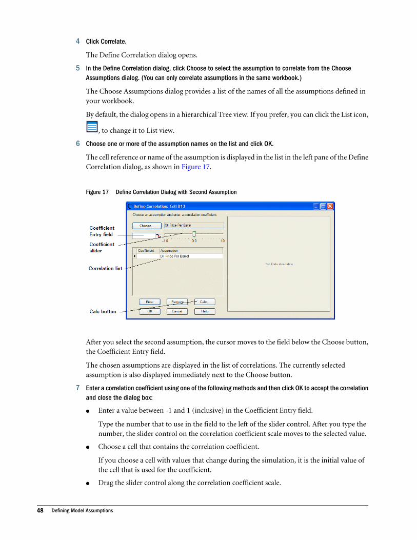
4 Click Correlate.
The Define Correlation dialog opens.
5 In the Define Correlation dialog, click Choose to select the assumption to correlate from the ChooseAssumptions dialog. (You can only correlate assumptions in the same workbook.)
The Choose Assumptions dialog provides a list of the names of all the assumptions defined inyour workbook.
By default, the dialog opens in a hierarchical Tree view. If you prefer, you can click the List icon,
, to change it to List view.
6 Choose one or more of the assumption names on the list and click OK.
The cell reference or name of the assumption is displayed in the list in the left pane of the DefineCorrelation dialog, as shown in Figure 17.
Figure 17 Define Correlation Dialog with Second Assumption
After you select the second assumption, the cursor moves to the field below the Choose button,the Coefficient Entry field.
The chosen assumptions are displayed in the list of correlations. The currently selectedassumption is also displayed immediately next to the Choose button.
7 Enter a correlation coefficient using one of the following methods and then click OK to accept the correlationand close the dialog box:
l Enter a value between -1 and 1 (inclusive) in the Coefficient Entry field.
Type the number that to use in the field to the left of the slider control. After you type thenumber, the slider control on the correlation coefficient scale moves to the selected value.
l Choose a cell that contains the correlation coefficient.
If you choose a cell with values that change during the simulation, it is the initial value ofthe cell that is used for the coefficient.
l Drag the slider control along the correlation coefficient scale.
48 Defining Model Assumptions
The value you select is displayed in the field to the left of the scale.
l Type the desired correlation coefficient in the Coefficient field in the correlation list.
l Click Calc.
A small dialog opens at the bottom of the first dialog. Enter the range of cells on yourspreadsheet that contains the empirical values that Crystal Ballshould use to calculate acorrelation coefficient.
Enter the range of cells in the standard A1:A2 format, where A designates the column and1 and 2 designate the first and last cell rows, respectively. For example, if one set of valuesis in column Q, rows 10 through 15 and the second set of values is in column R, rows 10through 15, enter the range in the left field as Q10:Q15 and the range in the right field asR10:R15.
Crystal Ball calculates the correlation coefficient, enters it in the field to the left of thecorrelation coefficient scale, and moves the slider control to the correct position.
The two cell ranges do not necessarily have to have the same dimensions, but they must containthe same number of value cells and must be in the same workbook. The cell ranges are read ina row-by-row fashion.
Each time you select a new assumption or correlation coefficient, Crystal Ball displays a samplecorrelation of the correlated assumption values in the chart to the right.
Figure 18 Correlation Chart
The points on the chart represent the pairing of assumption values as they would actually occurwhen running a simulation. The solid line running through the middle of the chart indicatesthe location where values of a perfect correlation (+1.0 or -1.0) would fall. The closer the pointsare to the solid line, the stronger the correlation.
In the example above, an Inflation Rate assumption and an Oil Price/Barrel assumption havebeen correlated using a coefficient of 0.8, a strong positive correlation. As the points on the chartshow, higher inflation values tend to be associated with higher oil prices and vice versa. Thischart can help you begin to understand how the two assumptions are related.
Additional Assumption Features 49
You can specify as many of these paired correlations as you want for each assumption, up to thetotal number of assumptions defined in a workbook.
You can generally ignore correlations between variables if one or both variables do not impactthe output or are not highly correlated.
Setting Assumption PreferencesThe Define Assumption dialog has a Preferences menu in the menubar. This menu has thefollowing main options:
Table 1 Preferences Menu, Define Assumptions Dialog Box
Setting Effect
Assumption Preferences Manage window display during simulations
Chart Preferences Determine the appearance of the assumption chart
The Chart Preferences settings are discussed in “Setting Chart Preferences” on page 112.
If you choose Assumption Preferences, the Assumption Preferences dialog opens.
You can use this dialog to:
l Choose a view for the assumption chart:
m Probability – shows a graph of all possible values for the assumption variable and theprobability of their occurrence.
m Cumulative Probability – shows a graph of the probability that the assumption variablewill fall at or below a given value.
m Reverse Cumulative Probability – shows a graph of the probability that the assumptionvariable will fall at or above a given value.
m Statistics – shows a table of measures of central tendency, variability, minimum andmaximum values, and other statistics for the assumption variable.
m Percentiles – shows a table of percentiles and their associated values for the assumptionvariable.
Note: For examples of each view, see “Changing the Distribution View and InterpretingStatistics” on page 102.
l Determine if and when the assumption chart window opens when a simulation runs.
To show the generated values in the window, turn on the Store Assumption Values ForSensitivity Analysis run preference. To do so, click the Run Preferences button, then click theOptions tab.
You can click Apply To to copy these settings to other assumptions. If necessary, you can clickDefaults to restore original default settings. When the settings are complete, click OK.
50 Defining Model Assumptions
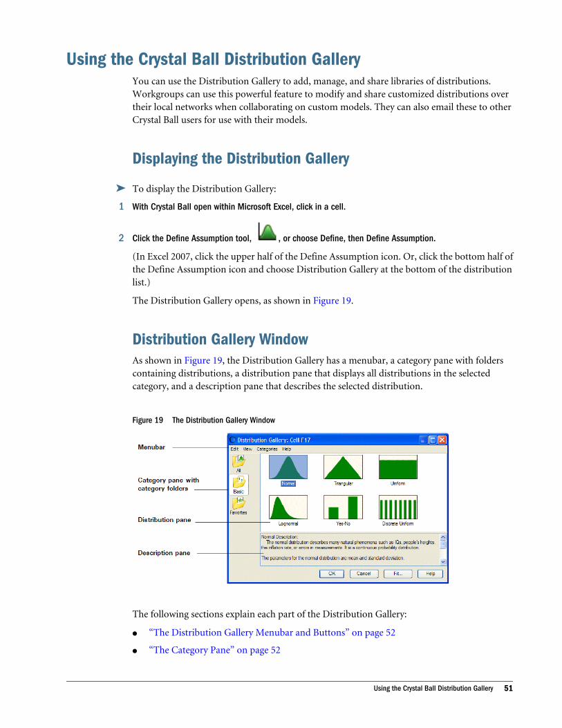
Using the Crystal Ball Distribution GalleryYou can use the Distribution Gallery to add, manage, and share libraries of distributions.Workgroups can use this powerful feature to modify and share customized distributions overtheir local networks when collaborating on custom models. They can also email these to otherCrystal Ball users for use with their models.
Displaying the Distribution Gallery
ä To display the Distribution Gallery:
1 With Crystal Ball open within Microsoft Excel, click in a cell.
2 Click the Define Assumption tool, , or choose Define, then Define Assumption.
(In Excel 2007, click the upper half of the Define Assumption icon. Or, click the bottom half ofthe Define Assumption icon and choose Distribution Gallery at the bottom of the distributionlist.)
The Distribution Gallery opens, as shown in Figure 19.
Distribution Gallery WindowAs shown in Figure 19, the Distribution Gallery has a menubar, a category pane with folderscontaining distributions, a distribution pane that displays all distributions in the selectedcategory, and a description pane that describes the selected distribution.
Figure 19 The Distribution Gallery Window
The following sections explain each part of the Distribution Gallery:
l “The Distribution Gallery Menubar and Buttons” on page 52
l “The Category Pane” on page 52
Using the Crystal Ball Distribution Gallery 51
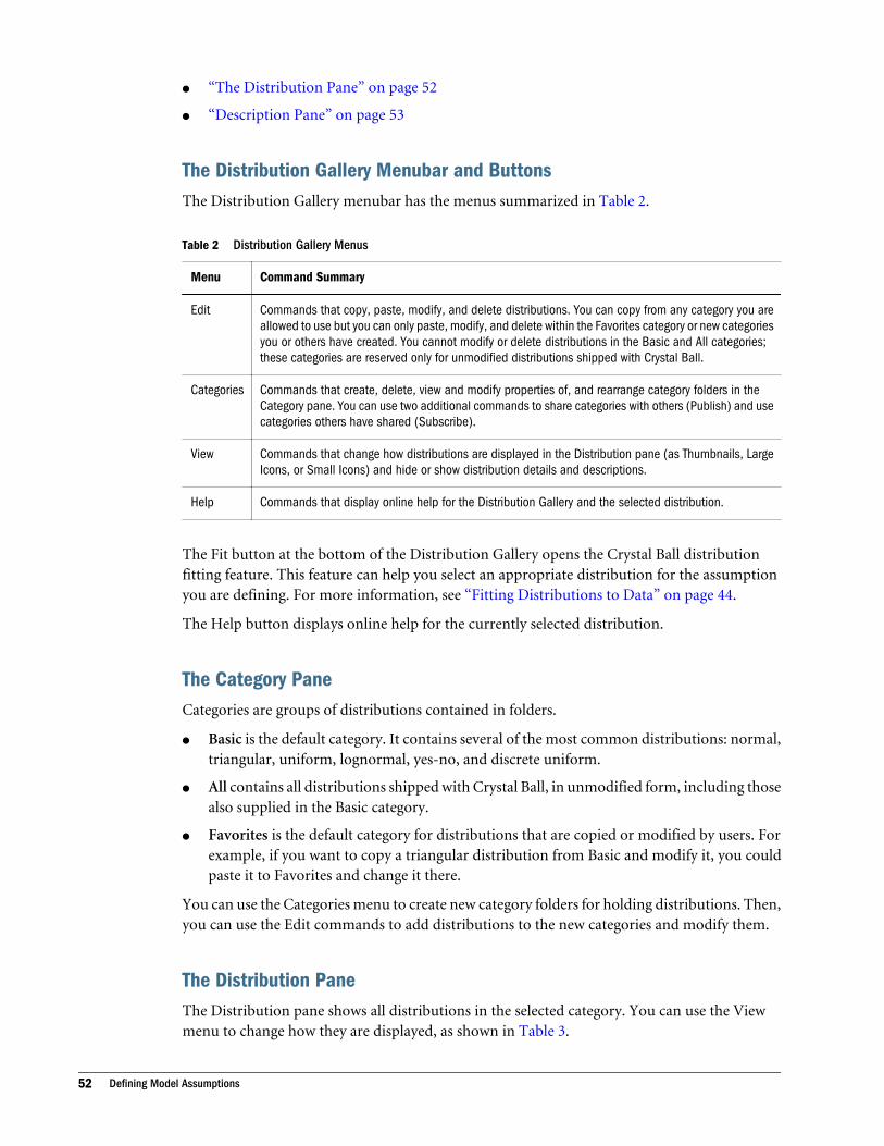
l “The Distribution Pane” on page 52
l “Description Pane” on page 53
The Distribution Gallery Menubar and ButtonsThe Distribution Gallery menubar has the menus summarized in Table 2.
Table 2 Distribution Gallery Menus
Menu Command Summary
Edit Commands that copy, paste, modify, and delete distributions. You can copy from any category you areallowed to use but you can only paste, modify, and delete within the Favorites category or new categoriesyou or others have created. You cannot modify or delete distributions in the Basic and All categories;these categories are reserved only for unmodified distributions shipped with Crystal Ball.
Categories Commands that create, delete, view and modify properties of, and rearrange category folders in theCategory pane. You can use two additional commands to share categories with others (Publish) and usecategories others have shared (Subscribe).
View Commands that change how distributions are displayed in the Distribution pane (as Thumbnails, LargeIcons, or Small Icons) and hide or show distribution details and descriptions.
Help Commands that display online help for the Distribution Gallery and the selected distribution.
The Fit button at the bottom of the Distribution Gallery opens the Crystal Ball distributionfitting feature. This feature can help you select an appropriate distribution for the assumptionyou are defining. For more information, see “Fitting Distributions to Data” on page 44.
The Help button displays online help for the currently selected distribution.
The Category PaneCategories are groups of distributions contained in folders.
l Basic is the default category. It contains several of the most common distributions: normal,triangular, uniform, lognormal, yes-no, and discrete uniform.
l All contains all distributions shipped with Crystal Ball, in unmodified form, including thosealso supplied in the Basic category.
l Favorites is the default category for distributions that are copied or modified by users. Forexample, if you want to copy a triangular distribution from Basic and modify it, you couldpaste it to Favorites and change it there.
You can use the Categories menu to create new category folders for holding distributions. Then,you can use the Edit commands to add distributions to the new categories and modify them.
The Distribution PaneThe Distribution pane shows all distributions in the selected category. You can use the Viewmenu to change how they are displayed, as shown in Table 3.
52 Defining Model Assumptions
Table 3 Distribution View Examples
View Command Example
Thumbnails
Large Icons
Small Icons
Details
Description PaneThe Description pane is displayed at the bottom of the Distribution Gallery and provides adetailed description of the selected distribution.
You can turn off Show Description in the View menu to show more distributions in theDistribution pane.
Managing DistributionsWorking with distributions is a key part of defining a model in Crystal Ball. Assumptions arethe main source of simulation input and distributions are the core component of assumptiondefinitions.
Several Crystal Ball features help you modify and save distributions for future use and sharethem with other Crystal Ball users:
l To create new distributions, see “Creating New Distributions” on page 54.
l To copy distributions, see “Copying and Pasting Distributions” on page 54.
l To paste distributions, see “Copying and Pasting Distributions” on page 54.
l To modify distributions, see “Modifying Distributions” on page 55.
l To modify distribution summaries and descriptions, see “Modifying DistributionSummaries and Descriptions” on page 55.
l To delete distributions, see “Deleting Distributions” on page 56.
l To set up pages for printing, see “Setting Up Distributions for Printing” on page 56.
l To print distribution information, see “Printing Distribution Information” on page 56.
Using the Crystal Ball Distribution Gallery 53
Creating New DistributionsYou can create new distributions by:
l Copying and renaming a distribution within the Distribution Gallery (“CreatingDistributions by Copying” on page 54)
l Defining a distribution in the Define Assumption dialog and adding it to the DistributionGallery (“Creating Distributions by Saving Assumptions” on page 54)
Creating Distributions by Copying
To create a distribution by copying another distribution, follow the steps in the next section,“Copying and Pasting Distributions” on page 54
Then, you can rename and modify the new distribution as needed.
Creating Distributions by Saving Assumptions
ä To create a distribution by saving an assumption:
1 With Crystal Ball running, click a cell in the spreadsheet.
It can be a value cell where you want to define an assumption or a blank cell.
2 Click the Define Assumption tool or choose Define, then Define Assumption.
3 Follow the steps in “Defining Assumptions” on page 38 to select a distribution and enter parameters.
4 Choose Edit, then Add To Gallery in the Define Assumption dialog.
5 The Add To Gallery dialog opens, where you can name the new distribution and select a category for it.
6 Click OK to save the distribution in the selected category.
If you created correlation data, it is not saved although the distribution type and any parametersettings are saved.
Now, the new distribution is available for use just as another other distribution, either suppliedwith Crystal Ball or user-defined.
Copying and Pasting Distributions
ä To copy and paste a distribution within Favorites or another user-defined category or from onecategory to another:
1 In the Distribution Gallery, click a category in the Category pane.
2 Click a distribution in the Distribution pane.
3 Choose Edit, then Copy or right-click and choose Copy from the right-click menu.
4 Click Favorites or another user-defined category in the Category pane.
5 Choose Edit, then Paste or right-click and choose Paste from the right-click menu.
54 Defining Model Assumptions
The distribution is pasted into the selected category. If another distribution in that category hadthe same name, the new distribution is displayed with the next larger number at the end. Forexample, if the category already had Normal1, a new normal distribution would be namedNormal2.
6 To rename the copied distribution, click its name and wait a moment. The name is highlighted for editing.
7 Type the new name and press Enter.
8 Modify the new distribution as needed.
Note: To easily copy a distribution from one category to another, select the category with thedistribution to copy. Then, drag the distribution into the closed category folder whereyou want to copy it. When you select that category, the copied distribution is displayedand you can rename it or modify it as described in the next section. However, thedistribution you copied remains in its original folder, unchanged.
Modifying DistributionsDistributions in the Basic or All categories are read-only and cannot be changed. However, afteryou have copied a distribution or used it to define an assumption, you can modify it in a numberof ways.
ä To modify a distribution:
1 Create a distribution as described in “Creating New Distributions” on page 54 and “Copying and PastingDistributions” on page 54.
2 Right-click the user-defined distribution and choose Modify (or click the distribution and choose Edit, thenModify in the Distribution Gallery menubar).
A prompt opens as a reminder that you are modifying a distribution and not defining anassumption.
3 Click OK to display the distribution in a window that looks like the Define Assumption dialog.
4 Modify the distribution as if it were an assumption, following the instructions in “Defining Assumptions” onpage 38.
5 When you are finished, click OK.
The modifications are saved with the distribution in the category and no assumption is createdin the spreadsheet.
Modifying Distribution Summaries and DescriptionsYou can edit the distribution Summary and Description text for any distribution in Favoritesor another user-defined category.
ä To modify Summary text for a distribution:
1 In the Distribution Gallery, set the View menu to Details.
Using the Crystal Ball Distribution Gallery 55
2 In the Distribution pane, right-click the Summary text to edit.
3 In the right-click menu, choose Modify Summary For distribution name.
4 When the Modify Summary dialog opens, enter the new text in the edit field and click OK.
The new text immediately replaces the original Summary text.
ä To modify Description text for a distribution:
1 Select the distribution in the Distribution Gallery.
2 Be sure View, then Show Description is checked.
3 Right-click the text in the Description pane.
4 In the right-click menu, choose Modify Description For distribution name.
5 When the Modify Description dialog opens, edit the description in the edit field and click OK.
(Alternately, you can just select the description text to modify and edit it. Be careful to avoidmodifying descriptions accidentally.)
The new text immediately replaces the original description.
Deleting DistributionsYou can delete a distribution in the Favorites category or other user-defined category. However,the original distribution of that type remains in Basic or All.
To delete a distribution, choose Edit, then Delete in the Distribution Gallery menubar, or right-click the distribution and choose Delete.
Setting Up Distributions for Printing
ä To select paper, print orientation, and margins before printing:
1 Double-click a distribution in the Distribution Gallery to display it in the Define Assumption dialog.
2 Choose Edit, then Page Setup in the Define Assumption menubar.
3 Set paper size and source, orientation, and margins.
4 Click OK to accept the settings.
Printing Distribution Information
ä To print a distribution:
1 Double-click a distribution in the Distribution Gallery to display it in the Define Assumption dialog.
2 Choose Edit, then Print in the Define Assumption menubar.
3 Confirm the printer and other settings.
4 Click OK to print the distribution.
56 Defining Model Assumptions
Printed information includes the chart with current parameter settings. The distribution nameand parameters are displayed in a box beneath the graphic.
You can preview before printing. In step 2, choose Edit, then Print Preview before you chooseEdit, then Print.
Managing CategoriesYou can use distribution categories to organize distributions and share them with other usersin your organization:
l To create new categories, see “Creating New Categories” on page 57.
l To view and edit category properties, see “Viewing and Editing Category Properties” onpage 58.
l To delete categories, see “Deleting Categories” on page 58.
l To rearrange category order, see “Rearranging Category Order” on page 58.
l To share categories over networks, see “Sharing Categories over Networks” on page 59.
l To use categories shared by others, see “Using Shared Categories” on page 59.
l To send and receive categories, see “Sharing Categories Through Email” on page 60.
l To edit shared categories, see “Editing Shared Categories” on page 60.
l To unpublish shared categories, see “Unpublishing Shared Categories” on page 61.
l To change distribution display within categories, see “The Distribution Pane” on page 52.
Creating New CategoriesYou can create a category of distributions to help with model development or to share with otherusers.
ä To create a category:
1 Choose Categories, then New.
The New Category dialog box opens.
2 Enter the name of your category. Optionally, you can enter a description, your name, and a version number(helpful for shared categories).
Note: If you enter an ampersand (&) before a letter in the category name, that letter becomes ashortcut key. You can then use it to select the category from the keyboard by holdingdown the Alt key and pressing the shortcut key. Shortcut keys are displayed underlinedwhen you press the Alt key. The new category should use a different shortcut key fromother categories.
3 Click OK.
The new folder is displayed in the Category pane and the category can be selected and used likeFavorites or any other user-defined category.
Using the Crystal Ball Distribution Gallery 57
Viewing and Editing Category PropertiesCategory properties include the information entered in the New Category dialog when a categoryis created. You can view properties for any category, but you can only edit properties for user-defined categories.
ä To view or edit properties:
1 Click a category in the Category pane.
2 Choose Categories, then Properties.
The Category Properties dialog opens.
3 Optional: Edit the information in any field that appears white. Read-only fields are gray.
4 When you have finished viewing or editing category properties, click OK.
The Category Properties dialog closes and any property changes are saved.
Deleting CategoriesYou can delete user-defined categories and all the distributions within them, but be careful notto delete a distribution you will need to use later.
ä To delete a category:
1 Select the category in the Category pane.
2 Choose Categories, then Delete.
A confirmation message is displayed.
3 When you click OK, the category and all its distributions are immediately deleted.
Original built-in distributions shipped with Crystal Ball are never deleted; only copies can bedeleted.
Rearranging Category OrderChanging the order of folders in the Category pane can be helpful if you want to arrangecategories in alphabetical order or put frequently used categories near the top.
ä To move a category folder:
1 Select the folder to move in the Category pane.
2 Choose Categories, then Move Up or Categories, then Move Down.
The folder moves up or down one position each time you choose the menu command.
3 Continue moving folders up and down until they are arranged as preferred.
58 Defining Model Assumptions
Sharing Categories over NetworksThe ability to publish and subscribe to categories is powerful. You can create large numbers ofspecific distributions, add them to a category, and then publish it on the network for other usersin your organization. Likewise, you can easily subscribe to categories published by others. Youcan also email categories to others and use categories sent to you.
ä To publish a category to a shared folder on your computer or to a location on a network:
1 Select a category in the Distribution Gallery.
2 Choose Categories, then Publish.
The Browse For Folder dialog opens.
3 Browse to locate the folder where you want to place the category. You can click + to expand a folder andview its subfolders. If you need to create a new folder, select the folder that should include the new folder.
The new folder is displayed and you can rename it. For example, if you want to create a folderunder My Documents, select My Documents. Then, when you click New Folder, the new folderis displayed under My Documents at the same level as My Pictures.
4 Click OK.
The dialog closes and a copy of your category is saved there.
Using Shared CategoriesIf other users have published categories in a shared folder on their computers or the network,you can access them for use with the Distribution Gallery. This is called subscribing to categories.
ä To subscribe to a category, learn its name and location, then:
1 Open the Distribution Gallery and choose Categories, then Subscribe.
The Subscribe To A Category dialog opens.
2 Click Add.
The Browse For Folder dialog opens.
3 Locate the target folder and click OK to add the new path to the Subscribe To A Category dialog box.
4 Click OK to load all categories in the listed paths and close the Subscribe To A Category dialog box.
All loaded categories are available for use as if they were on your local computer.
Note: Shared categories can be used like local categories in most ways. However, they cannotbe modified unless they also exist in a folder on your local computer. If several users copya published category locally and then modify it, they can publish their own versions andoverwrite each others’ changes. If you are publishing a category, you might want to makethe shared folder read-only to avoid this problem.
ä To edit or delete a path, or rearrange the path order:
1 Open the Subscribe To A Category dialog as described in step 2 above.
Using the Crystal Ball Distribution Gallery 59
2 Select the path to a target category.
3 Click an action button: Edit, Delete, Move Up, or Move Down.
4 When you are finished, click OK.
If you delete a path to a subscribed category, that category disappears from the Category paneof the Distribution Gallery. You can resubscribe to it at any time to use it again.
Sharing Categories Through EmailYou can use email to share a user-defined category with a Crystal Ball user who is not on yournetwork.
ä To share categories using email:
1 Create and address an email message.
2 Use the file attachment command and browse to the category folder on your machine.
By default, this is C:\Documents and Settings\your username\Application Data\Oracle\CrystalBall\11.0\Store.
3 Select the user-defined category to send.
Crystal Ball category files have this format: CBCategory_name.cbc. For example, the Favoritescategory The Browse For Folder dialog opens. as CBCategory_Favorites.cbc.
4 Send the email.
ä To use a category received in an email:
1 Open the email.
2 Save the attachment in the Crystal Balll category folder, by default C:\Documents and Settings\yourusername\Application Data\Oracle\Crystal Ball\11.0\Store.
The next time you start Crystal Ball, the new category is displayed in the Category pane of theDistribution Gallery.
Alternately, you can save the attachment in another folder, then follow the steps in “Using SharedCategories” on page 59 to subscribe to it.
Editing Shared Categories
ä To edit a published user-defined category:
1 Make the changes in your Distribution Gallery.
2 Follow the steps in “Sharing Categories over Networks” on page 59 to publish the category to the sameplace.
3 When you are prompted to overwrite the existing file, click OK.
This publishes the modified category. Now, the next time a subscriber loads Crystal Ball, themodified category is displayed in the Distribution Gallery.
60 Defining Model Assumptions
Unpublishing Shared Categories
ä If you have published a user-defined category and want to remove it from publication, or"unpublish" it:
1 Use My Computer or Windows Explorer to browse to the folder where the category was published.
The category file is displayed as CBCategory_name.cbc. For example, the Favorites category isdisplayed as CBCategory_Favorites.cbc.
2 Select the category file and delete it.
The next time a subscriber loads Crystal Ball, the deleted category will not be displayed in theDistribution Gallery. Existing assumptions based on distributions from that category will stillwork but those distributions won’t be available for creating new assumptions.
A Note About Modifying Shared CategoriesIf a shared category is moved, deleted, or otherwise modified, subscribers to that category willnot notice the changes until they close Crystal Ball and open it again. It is wise to notifysubscribers when a change of that type occurs so they can start a new Crystal Ball session andrefresh their view of the Distribution Gallery.
Using the Crystal Ball Distribution Gallery 61

62 Defining Model Assumptions
4Defining Other Model Elements
In This Chapter
Introduction... . . . . . . . . . . . . . . . . . . . . . . . . . . . . . . . . . . . . . . . . . . . . . . . . . . . . . . . . . . . . . . . . . . . . . . . . . . . . . . . . . . . . . . . . . . . . . . . . . . . . . . . . . . . . . . . . . . . . . .63
Defining Decision Variable Cells .. . . . . . . . . . . . . . . . . . . . . . . . . . . . . . . . . . . . . . . . . . . . . . . . . . . . . . . . . . . . . . . . . . . . . . . . . . . . . . . . . . . . . . . . . . . . . . . . .63
Defining Forecasts .. . . . . . . . . . . . . . . . . . . . . . . . . . . . . . . . . . . . . . . . . . . . . . . . . . . . . . . . . . . . . . . . . . . . . . . . . . . . . . . . . . . . . . . . . . . . . . . . . . . . . . . . . . . . . . . .64
Working with Crystal Ball Data... . . . . . . . . . . . . . . . . . . . . . . . . . . . . . . . . . . . . . . . . . . . . . . . . . . . . . . . . . . . . . . . . . . . . . . . . . . . . . . . . . . . . . . . . . . . . . . . . .68
Setting Cell Preferences ... . . . . . . . . . . . . . . . . . . . . . . . . . . . . . . . . . . . . . . . . . . . . . . . . . . . . . . . . . . . . . . . . . . . . . . . . . . . . . . . . . . . . . . . . . . . . . . . . . . . . . . . .72
Saving and Restoring Models.. . . . . . . . . . . . . . . . . . . . . . . . . . . . . . . . . . . . . . . . . . . . . . . . . . . . . . . . . . . . . . . . . . . . . . . . . . . . . . . . . . . . . . . . . . . . . . . . . . . .73
IntroductionChapter 3 describes how to start building a spreadsheet model by defining assumption cells. Thischapter provides step-by-step instructions for completing models in Crystal Ball so you can runsimulations against them. As you work through these instructions, you will learn to definedecision variable cells and forecasts and how to cut, copy, and paste Crystal Ball data.
After you complete this chapter, read Chapter 5, “Running Simulations” for information onsetting run preferences and running simulations.
Defining Decision Variable CellsDecision variables are the variables that you can control, such as rent to charge or the amountof money to invest. Decision variables are not required for simulation models, but they can beuseful when comparing and optimizing alternate scenarios. Several of the Crystal Ball toolsdiscussed in Chapter 9, “Crystal Ball Tools”, use and benefit from decision variables.
You also use decision variables with OptQuest, if available.
ä To define one or more decision variable cells:
1 Select a cell or range of cells.
Select value cells or blank cells only. You cannot define a decision on a formula or non-numericcell.
2 Select Define , then Define Decision, .
The Define Decision Variable dialog opens .
Introduction 63
3 Click the More button, , to display all settings.
4 Complete the Define Decision Variable dialog:
l Name is the name of the decision variable.
l Bounds are the upper and lower limits for the decision variable range.
l Type defines whether the variable type is:
m Continuous — can assume any value between the lower and upper bounds
m Discrete — can assume values at specific intervals between the lower and upper bounds
With Discrete selected, Step specifies the interval between values for discrete variables.For example Step = 1 could be used to specify whole dollars, while Step = .5 could specify50-cent increments.
m Binary — is 0 or 1 to represent a yes-no decision, where 0 = no and 1 = yes
m Category — can assume any discrete integer between the lower and upper bounds(inclusive), where the order of the values does not matter. This type, used for attributesor indexes, is mostly used when numeric values represent conditions or groups insteadof numeric values. Example model Groundwater Cleanup.xls contains a decisionvariable named Remediation Method, expressed as integers 1, 2, and 3. These are notnumeric values, but instead they represent three different remediation methods forgroundwater cleanup and can be defined using the Category type.
m Custom — can assume any value from a list of two or more specific values or a cell rangereference. When values are entered directly, separate them by a valid list separator — acomma, semicolon, or other value specified in the Windows regional and languagesettings. If a cell range reference is used, it must include more than one cell so there willbe two or more values. Blanks and non-numerical values in the range are ignored.
You can use cell referencing to name a decision variable, define the lower and upperlimits, set the step size, and define custom values (“ Entering Cell References andFormulas” on page 42).
5 Click OK.
6 Repeat these steps for each decision variable in your model.
Note: There is no absolute limit to the number of data cells you can define per worksheet. Ingeneral, you should define less than 1000 assumptions, decision variables, and forecastsper worksheet.
Defining ForecastsAfter you define the assumption cells and decision variables, you are ready to select and defineforecast cells. Forecast cells usually contain formulas that refer to one or more assumption anddecision variable cells. The forecast cells combine cells in your model to produce the results youneed.
64 Defining Other Model Elements
ä To define forecast cells:
1 Select a formula cell or a range of formula cells.
2 Select Define, then Define Forecast, .
The Define Forecast dialog opens .
If you have activated Crystal Ball’s process capability features, additional fields are displayed.These are described in “Setting Specification Limits and Targets” on page 387.
3 Complete the Define Forecast dialog:
l Name is the name of the forecast.
l Units is the name of the units that are displayed at the bottom of the forecast chart, such asMillions.
4 To set additional forecast preferences, click the More button, , to expand the Define Forecast dialog.
The expanded Define Forecast dialog has four tabs of additional options and fields, listed in“Setting Forecast Preferences” on page 65.
5 Click OK.
6 Repeat steps 1–4 for each forecast in your model.
Clicking Defaults in the expanded Define Forecast dialog restores the original default settingsin place of any new settings you have made. You can also click Apply To to use the settings inother charts and worksheets.
Setting Forecast Preferences
The forecast preference settings are displayed when you click the More button, , in the DefineForecast dialog box or select Preferences , then Forecast in a forecast chart menu bar. The tabsin this dialog control several important aspects of Crystal Ball:
l “Forecast Window Tab” on page 66 — window display and distribution fitting for theforecast
l “Precision Tab” on page 66 — precision control settings
l “Filter Tab” on page 67 — value filtering, which discards values inside or outside a rangefor the current forecast
l “Auto Extract Tab” on page 67 — automatic data extraction to Excel when a simulationstops.
Note: See "Confidence intervals" in the "Statistical Definitions" chapter of the online OracleCrystal Ball Statistical Guide for more information about how absolute and relativeprecision relate to the confidence interval.
When you expand the Define Forecast dialog or open the Forecast Preferences dialog, theForecast Window tab is displayed by default.
Defining Forecasts 65

Forecast Window TabThe Forecast Window tab of the Forecast Preferences dialog offers the following settings tomanage window display and distribution fitting for the forecast:
l View settings — Set the forecast window’s display type (“Changing the Distribution Viewand Interpreting Statistics” on page 102).
l Window settings — Set whether to display the forecast window automatically while thesimulation runs or when the simulation stops. You can display one or more forecasts whilethe simulation is running. If you decide not to display the forecast, the simulation continuesto run. You can override this option and close all the forecast windows using the SuppressForecast Windows option in the Run Preferences dialog (“Setting Run Preferences” on page76).
m Window, then While Running Simulation — Displays the forecast windowautomatically during simulations. This slows down the simulation.
m Window, then When Simulation Stops — Displays the forecast window automaticallyafter the simulation stops. This is faster than displaying the window during simulations.
l Fit Distribution — Fits a probability distribution to the forecast. After selecting thischeckbox in this group, you can click Fit Options to select the distribution and goodness-of-fit tests you want.
Click OK to apply settings on the current tab to the active forecast. Or, you can click Apply Toto apply settings on the active tab to the active worksheet, the active workbook, or all workbooks.At any time, you can click Defaults to restore the original default settings on the active tab in thedialog.
Precision TabThe Precision tab of the Forecast Preferences dialog manages the precision control settings thatdetermine when to stop a simulation based on confidence intervals for selected statistics.
The current simulation must be reset before precision control settings will take effect.
Select from the following settings:
l Specify The Desired Precision For Forecast Statistics — Activates the precision controlsettings for the forecast. Crystal Ball uses these settings only if the simulation is set to stopwhen it reaches the specified precision from the Run Preferences dialog (“Setting RunPreferences” on page 76). The statistics available for precision control are the mean, thestandard deviation, and an indicated percentile. Check any or all. If you select Percentile,you can enter any percentile value greater than 0 and less than 100 to use as a precisioncontrol statistic.
l Must Be Within Plus Or Minus — Selects which range to use for precision control, absoluteunits or relative percentage.
m Units — Determines the size of the confidence interval, in actual forecast units, used totest the precision of the forecast statistics.
66 Defining Other Model Elements
m Percent — Determines the size of the confidence interval, in percentage terms, used totest the precision of the forecast statistics.
Click OK to apply settings on the current tab to the active forecast. Or, you can click Apply Toto apply settings on the active tab to the active worksheet, the active workbook, or all workbooks.At any time, you can click Defaults to restore the original default settings on the active tab in thedialog.
Filter TabYou can use the Filter tab of the Forecast Preferences dialog to discard values inside or outsidea range for the current forecast or globally for all forecasts in a model. The values are notpermanently deleted, only discarded for the purposes of your current analysis.
Select from the following settings:
l Set A Filter On The Forecast Values — Activates the filter settings for the forecast.
l Include Values In The Range — Discards values from the forecast if they fall above or belowthe two values in the range fields. Endpoints are included, not excluded.
l Exclude Values In The Range — Discards values from the forecast if they fall between thetwo values in the range fields. The range is inclusive; Crystal Ball discards values inside therange as well as values equal to the range endpoints.
l When filtering values for this forecast, remove values for the same trial from other forecaststoo — For each trial that a value is not included or is excluded, removes the value for thattrial from all other forecasts in the model, and assumptions too. For example, if the filterfor the current forecast is set to include values from 4 through 10 and the value for the thirdtrial is 12, the value for the third trial will be filtered from the current forecast and all otherforecasts and assumptions in the model, regardless of the values in the other forecasts. If thissetting is checked and you run a Forecasts report, "globally filtered" is displayed for theforecast in the Summary data following the filter description.
Note: This setting can be checked in the Define Forecast dialog for several forecasts withdifferent filter settings. In that case, filtering for each selected forecast will be appliedacross all forecasts.
Click OK to apply settings on the current tab to the active forecast. Or, you can click Apply Toto apply settings on the active tab to the active worksheet, the active workbook, or all workbooks.At any time, you can click Defaults to restore the original default settings on the active tab in thedialog.
Auto Extract TabYou can use the Auto Extract tab of the Forecast Preferences dialog to specify which statistics toextract automatically to Excel after the simulation stops.
The Auto Extract settings create tables of unformatted statistics primarily for use in otheranalyses. To extract formatted data, see “Extracting Data” on page 161.
You can choose from the following settings:
Defining Forecasts 67
l Extract forecast statistics automatically to your spreadsheet when the simulation stops— Activates the auto-extract feature.
l [listbox at the left] — The list of statistics you can extract. Check the statistics you want,then use the up and down arrows to rearrange their order, if you want.
l Starting Cell — The first cell on the forecast’s worksheet where the statistics will be copied.Be sure no data entries are displayed to the right of this cell and below it because data couldbe overwritten without warning.
l Formatting — Whether to include labels on the extracted statistics and use Excel’sAutoFormat for the cells.
l Direction — Whether the extraction proceeds vertically (downward) or horizontally (to theright) on the worksheet.
Click OK to apply settings on the current tab to the active forecast. Or, you can click Apply Toto apply settings on the active tab to the active worksheet, the active workbook, or all workbooks.At any time, you can click Defaults to restore the original default settings on the active tab in thedialog.
Working with Crystal Ball DataYou can use special commands to copy, paste, and clear Crystal Ball cell definitions from cells.These are different from similar Excel commands and must be used to copy Crystal Ball celldefinitions (data). Other Crystal Ball commands select data and highlight it for your review.
The following sections describe these special commands:
l “Editing Crystal Ball Data” on page 68
l “Selecting and Reviewing Data” on page 70
Editing Crystal Ball DataYou can use the edit commands to copy, paste, or clear assumptions, decision variables, orforecasts from cells. You can set up an entire row or column of assumptions, decision variables,or forecasts with just a few steps.
If you select a range of cells with more than one kind of Crystal Ball data — for example, anassumption and a forecast — Crystal Ball prompts for which data type to copy or clear.
Important! To copy Crystal Ball cell definitions, use only the Crystal Ball Copy Data, Paste Data,or Clear Data commands. Using the Excel copy and paste commands only copies the cell valueand attributes, including cell color or pattern.
The following sections describe how to edit Crystal Ball data:
l “Copying Crystal Ball Data” on page 69
l “Pasting Crystal Ball Data” on page 69
l “Clearing Crystal Ball Data” on page 69
l “Clearing All Crystal Ball Data of a Single Type” on page 70
68 Defining Other Model Elements
Copying Crystal Ball Data
ä To copy Crystal Ball assumptions, decision variables, or forecasts from one area of thespreadsheet to another area in the same workbook or a different workbook:
1 Select a cell or a range of cells that contains the Crystal Ball data to copy.
2 Select Define, then Copy [Data], .
If you select a range of cells with more than one kind of Crystal Ball data — for example, anassumption and a forecast — Crystal Ball prompts for which data type to copy.
3 Check the type or types to copy and click OK.
Pasting Crystal Ball Data
ä To paste Crystal Ball data:
1 Select a cell or a range of cells that to paste into.
It should contain cells with values if you are pasting assumptions or decision variables (unlessthe range is all blank; see note below) and cells with formulas if you are pasting forecasts.
If you are pasting assumptions or decision variables into a completely blank range of cells, CrystalBall pastes them along with the underlying cell value from each copied cell. Forecasts must bepasted into a cell with a formula.
2 Choose Define, then Paste [Data], .
Crystal Ball pastes all selected data types (assumptions, decision variables, and forecasts) fromthe copied range into the range selected in step 1. Any existing Crystal Ball data in the rangeselected for pasting will be overwritten.
For best results, use the Paste Data command immediately after the Copy Data command. Youare probably already familiar with this from using Excel; if you copy in Excel and then do anythingelse but select a range for pasting, the copied area is unselected and you must select it again beforecontinuing.
Clearing Crystal Ball Data
ä To clear Crystal Ball data:
1 Select a cell or a range of cells that contains the Crystal Ball data to clear.
2 Select Define, then Clear [Data], .
If you select a range of cells with more than one kind of Crystal Ball data — for example, anassumption and a forecast — Crystal Ball prompts for which data type to clear.
3 Check the type or types to clear and click OK.
Working with Crystal Ball Data 69
Crystal Ball clears the selected Crystal Ball data type (assumptions, decision variables, andforecast definitions) from each cell.
Clearing All Crystal Ball Data of a Single Type
ä To clear all of one type of Crystal Ball data from all cells in the active worksheet:
1 Select one of the following options:
l Define, then Select All Assumptions
l Define, then Select All Decisions
l Define, then Select All Forecasts
(In Excel 2007, choose Define , then Select and then choose one of the Select commands.)
2 Select Define, then Clear [Data], .
Crystal Ball clears the Crystal Ball data from all the selected cells in the active worksheet.
Edit, then Clear, then All also clears all Crystal Balldata from selected cells.
Selecting and Reviewing DataAfter you define assumptions, decision variables, and forecast cells and return to the spreadsheet,you might want to check the cell definitions to make sure you have defined them as you intended.You can select all the assumption, forecast, and decision variable cells and check theircorresponding dialogs in sequence.
The following sections describe how to review and select Crystal Ball data:
l “Reviewing Assumption Cells” on page 70
l “Reviewing Decision Variable Cells” on page 71
l “Reviewing Forecast Cells” on page 71
l “Reviewing Selected Cells” on page 72
Note: Regarding the following sections concerning selection, in Excel 2007, choose Define, thenSelect and then choose one of the Select commands.
Reviewing Assumption Cells
ä To review all assumption cells:
1 Select Define, then Select All Assumptions, .
Crystal Ball selects each cell defined as an assumption.
70 Defining Other Model Elements
2 Select Define, then Define Assumption, .
The distribution dialog for the first assumption cell opens .
3 Optional: Change the assumption parameters.
4 Click OK.
If you have more than one assumption cell, each assumption is displayed in turn. Repeat steps3 and 4 to check the assumptions for each cell.
Reviewing Decision Variable Cells
ä To review all decision variable cells:
1 Select Define, then Select All Decisions, .
Crystal Ball selects each cell defined as a decision variable.
2 Select Define, then Define Decision, .
The Define Decision Variable dialog for the first decision variable cell opens.
3 Optional: Change the decision variable parameters.
4 Click OK.
If you have more than one decision variable cell, each decision variable opens in turn. Repeatsteps 3 and 4 to check the decision variables for each cell.
Reviewing Forecast Cells
ä To review all forecast cells:
1 Select Define, then Select All Forecasts, .
Crystal Ball selects each cell defined as a forecast.
2 Select Define, then Define Forecast, .
The forecast dialog for the first forecast cell opens.
3 Optional: Change the forecast definition.
4 Click OK.
If you have selected more than one forecast cell, each forecast is displayed in turn. Repeat steps3 and 4 to check the forecast for each cell.
Working with Crystal Ball Data 71
Reviewing Selected Cells
ä To review Crystal Ball data cells on any open workbook:
1 Select Define, then Select.
The Select dialog opens.
By default, the dialog opens in hierarchical Tree view. All the assumptions are listed first, thenall the decision variables, and finally all the forecasts.
You can click the Assumption, Decision Variable, and Forecast buttons to show and hideassumptions, decision variables, and forecasts, respectively. If you prefer to view available cells
in list format, click the List button, .
2 Check the cells to select.
3 Click OK to highlight all the selected cells so you can change their preferences or perform other actions onthem.
You can use the Select dialog to select cells on more than one worksheet but you need to activateeach worksheet in turn to review and, if desired, apply a command to all the selected cells.
Setting Cell PreferencesYou can change the appearance of Crystal Ball assumption, forecast, and decision variable cellsso you can quickly identify them on your spreadsheets. You can set Crystal Ball to change theappearance of these cells as you define them, or you can change the appearance of predefinedcells.
ä To set cell preferences:
1 Choose Define, then Cell Preferences.
(In Excel 2007, choose Define, then Cell Prefs.)
The Cell Preferences dialog opens.
2 Click the tab for the kind of cell to format: Assumptions, Decision Variables, or Forecasts.
3 Make appropriate settings for the chosen cell type:
l Color — Changes the color of each Crystal Ball data cell of the type modified by the selectedtab.
l Pattern — Changes the pattern of each Crystal Ball data cell of the type modified by theselected tab.
l Add Comment To Cell — Adds an Excel comment that provides more information aboutthe Crystal Ball data within each cell. (Crystal Ball only updates cell comments when youdefine or redefine an assumption, decision variable, or forecast.)
l Set Cell Value To... — Changes assumption cell values to the selected value (Mean orMedian) when no simulation is running.
72 Defining Other Model Elements
l Set To Range Midpoint — Changes decision variable cell values to the selected value (rangeMidpoint, Minimum, or Maximum) when no simulation is running.
4 Click Apply To and choose whether to apply settings from only the current tab or all tabs in the Cell Preferencesdialog.
5 Choose whether to apply the settings to all cell preferences of the chosen type(s) on the current Excelworksheet, all worksheets in the current workbook, or all open workbooks and any new workbooks to becreated later.
(The default is All Open And New Workbooks.)
6 Click OK to close the Apply To dialog and apply the settings to the chosen cell types and worksheets.
Note: Like some other preferences, cell preferences must be applied to all cells of the selectedtype(s) on the chosen worksheet(s) or workbook(s). If necessary, you can click theDefaults button before choosing Apply To to clear your cell preference settings and restorethe original defaults.
Saving and Restoring ModelsThe distributions specified for each assumption cell, the settings specified for each forecast cell,and the range information for each decision variable cell are saved with their spreadsheet throughthe Excel save process. When you open the spreadsheet again, Crystal Ball retains yourassumption, forecast, and decision variable cells.
Note: When you run simulations, as described in the next chapter, you can also save and restoresimulation results in a separate file for future display and analysis (“Saving and RestoringSimulation Results” on page 86).
Saving and Restoring Models 73

74 Defining Other Model Elements
5Running Simulations
In This Chapter
Introduction... . . . . . . . . . . . . . . . . . . . . . . . . . . . . . . . . . . . . . . . . . . . . . . . . . . . . . . . . . . . . . . . . . . . . . . . . . . . . . . . . . . . . . . . . . . . . . . . . . . . . . . . . . . . . . . . . . . . . . .75
About Crystal Ball Simulations... . . . . . . . . . . . . . . . . . . . . . . . . . . . . . . . . . . . . . . . . . . . . . . . . . . . . . . . . . . . . . . . . . . . . . . . . . . . . . . . . . . . . . . . . . . . . . . . . .75
Setting Run Preferences ... . . . . . . . . . . . . . . . . . . . . . . . . . . . . . . . . . . . . . . . . . . . . . . . . . . . . . . . . . . . . . . . . . . . . . . . . . . . . . . . . . . . . . . . . . . . . . . . . . . . . . . .76
Freezing Crystal Ball Data Cells.. . . . . . . . . . . . . . . . . . . . . . . . . . . . . . . . . . . . . . . . . . . . . . . . . . . . . . . . . . . . . . . . . . . . . . . . . . . . . . . . . . . . . . . . . . . . . . . . . .80
Running Simulations... . . . . . . . . . . . . . . . . . . . . . . . . . . . . . . . . . . . . . . . . . . . . . . . . . . . . . . . . . . . . . . . . . . . . . . . . . . . . . . . . . . . . . . . . . . . . . . . . . . . . . . . . . . . .81
Managing Chart Windows ... . . . . . . . . . . . . . . . . . . . . . . . . . . . . . . . . . . . . . . . . . . . . . . . . . . . . . . . . . . . . . . . . . . . . . . . . . . . . . . . . . . . . . . . . . . . . . . . . . . . . . .84
Saving and Restoring Simulation Results.. . . . . . . . . . . . . . . . . . . . . . . . . . . . . . . . . . . . . . . . . . . . . . . . . . . . . . . . . . . . . . . . . . . . . . . . . . . . . . . . . . . . . . .86
Functions for Use in Excel Models.. . . . . . . . . . . . . . . . . . . . . . . . . . . . . . . . . . . . . . . . . . . . . . . . . . . . . . . . . . . . . . . . . . . . . . . . . . . . . . . . . . . . . . . . . . . . . . .88
Running User-Defined Macros ... . . . . . . . . . . . . . . . . . . . . . . . . . . . . . . . . . . . . . . . . . . . . . . . . . . . . . . . . . . . . . . . . . . . . . . . . . . . . . . . . . . . . . . . . . . . . . . . . .88
IntroductionChapter 3 and Chapter 4 describe how to define a spreadsheet model in Crystal Ball. This chapterprovides step-by-step instructions for setting run preferences and running a simulation inCrystal Ball.
After you complete this chapter, read Chapter 6 for information about analyzing simulationresults.
About Crystal Ball SimulationsAfter you define assumption, forecast, and decision variable cells in your spreadsheet model,you are ready to run the simulation. Crystal Ball uses a technique called Monte Carlo simulationto forecast the entire range of results most likely to occur in the model scenario. For moreinformation on Monte Carlo simulation, see “Monte Carlo Simulation and Crystal Ball” on page20.
Crystal Ball provides statistics that describe the forecast results. For more information on forecastresults and statistics, see Chapter 6, “Analyzing Forecast Charts,”and the "Statistical Definitions"chapter of the Oracle Crystal Ball Statistical Guide.
To run simulations in Crystal Ball, follow these basic steps:
1. Define assumptions (“Entering Assumptions” on page 38), forecasts (“Defining Forecasts”on page 64), and decision variable cells if appropriate (“Defining Decision Variable Cells”on page 63).
Introduction 75
2. If you want, customize the appearance of each cell as described in “Setting Cell Preferences”on page 72.
3. Set run preferences as described in the next section, “Setting Run Preferences” on page76.
4. Optionally, exclude certain data cells from the simulation by “freezing” them, described in“Freezing Crystal Ball Data Cells” on page 80.
5. Run the simulation as described in “Running Simulations” on page 81.
The following sections explain each step.
Setting Run PreferencesRun preferences determine how Crystal Ball runs a simulation.
ä To change run preferences:
1 Reset the previous simulation, if necessary, .
2 Choose Run, then Run Preferences to display the Run Preferences dialog, .
3 Click the tab with the preferences to change, described in the following sections:
l “Setting Trials Preferences” on page 76 — Specify when to stop a simulation, namelynumber of trials, calculation errors, and precision control.
l “Setting Sampling Preferences” on page 77 — Set the sampling seed value, method, andsample size.
l “Setting Speed Preferences” on page 78 — Determine whether a simulation runs inNormal, Demo, or Extreme (if available) and set additional speed control options.
l “Setting Options Preferences” on page 79 — Set a number of run preferences, includingwhether sensitivity data and assumption values are stored, whether assumption correlationsare activated, whether user macros are run, whether low memory triggers, a warning, andwhether the Crystal Ball Control Panel opens.
l “Setting Statistics Preferences” on page 80 — Determine how Crystal Ball displayspercentiles and activates process capability features.
4 Change any preferences on any tab.
5 Click OK.
6 To reset settings on the active tab to the original defaults, click Defaults.
Setting Trials PreferencesThe Trials tab of the Run Preferences dialog sets preferences that stop a simulation: number oftrials, calculation errors, and precision control. For general instructions, see “Setting RunPreferences” on page 76.
76 Running Simulations
The current simulation must be reset before precision control settings will take effect.
The Trials tab of the Run Preferences dialog has these settings:
l Number Of Trials To Run — Defines the maximum number of trials that Crystal Ball runsbefore it stops the simulation. If you check either of the checkboxes on this dialog, CrystalBall only uses the maximum number of trials if forecast results do not meet the other stopcriteria first.
l Stop On Calculation Errors — When checked, stops the simulation when a mathematicalerror (such as division by zero) occurs in any forecast cell. If a calculation error occurs, tohelp you find the error, Crystal Ball does not restore the cell values. If no calculation errorsoccur, the simulation continues until it reaches the Number Of Trials To Run or (if set)when the specified precision is reached.
Note: In Extreme Speed, the simulation stops at the end of a burst of trials when an erroroccurs, and not immediately upon detecting the error.
l Stop When Precision Control Limits Are Reached — When checked stops the simulationwhen certain statistics reach a specified level of precision. You choose the statistics and definethe precision that triggers this option in each Define Forecast dialog. For instructions, see“Precision Tab” on page 66. Any forecasts set to use precision control must all reach theirspecified precision within the confidence level to stop the simulation. If all the forecasts setto use precision control don’t meet the specified precision, the simulation stops when itreaches the Number Of Trials To Run. By default, precision control is on.
l Confidence Level — Sets the precision level (confidence level) that indicates when to stopa simulation.
Setting Sampling PreferencesThe Sampling tab of the Run Preferences dialog sets the sampling seed value, sampling method,and sample size. For general instructions, see “Setting Run Preferences” on page 76.
The Sampling tab of the Run Preferences dialog has these settings:
l Use Same Sequence Of Random Numbers — Sets the random number generator to generatethe same set of random numbers for assumptions, so you can repeat simulation results.When you select this option, enter an integer seed value in the Initial Seed Value field.
l Initial Seed Value — Determines the first number in the sequence of random numbersgenerated for the assumption cells (integer).
Note: To reproduce the sample results shown in this manual, check Use Same Sequence OfRandom Numbers and use a seed value of 999.
l Sampling Method — Indicates whether to use Monte Carlo or Latin Hypercube simulationsampling. Latin Hypercube sampling generates values more evenly and consistently acrossthe distribution, but requires more memory.
Setting Run Preferences 77
l Sample Size — For Latin Hypercube sampling, divides each distribution into the specifiednumber of intervals (bins). A higher number increases the evenness of the sampling method,while reducing the randomness.
Note: If you are using Excel 2007 with multi-threading, there is no guaranteed order ofexecution for user-defined functions included in Crystal Ball models. For this reason,they will not always return consistent results, even if a seed is set.
Setting Speed PreferencesThe Speed tab of the Run Preferences dialog adjusts how fast a simulation runs. Extreme speedis only available in Crystal Ball Decision Optimizer. Extreme speed is the default simulationspeed, if it is available. Otherwise, Crystal Ball only runs in Normal or Demo speed. If you chooseNormal or Demo speed, the Options button is active and you can make additional settings.
Note: If your license includes Extreme speed, be sure to read Appendix C, “Using the ExtremeSpeed Feature” on page 311, for important information about model compatibility.
For general instructions, see “Setting Run Preferences” on page 76.
The Speed tab of the Run Preferences dialog has these settings:
l Run Mode settings — Determine overall simulation speed.
m Extreme Speed — Available as a Crystal Ball option. This setting runs simulations upto 100 times faster than Normal mode but is not suitable for some models. For details,see Appendix C, “Using the Extreme Speed Feature” on page 311.
m Normal Speed — The standard simulation option for general model processing.
m Demo Speed — Runs simulations in "slow-motion" to make it easier to watch valueschange in spreadsheet cells and charts.
l Options settings — Set update rules for the active worksheet (Normal and Demo speedsonly). See “Speed Tab Options Settings” on page 78 for details.
l Chart Windows settings — Set the redraw rate for any charts open during a simulation.
m Redraw Every _ Seconds — Defines the redraw rate in terms of time. The default valueis 0.5.
m Suppress Chart Windows (Fastest) — Closes all charts during simulation. Selecting thisoption overrides the Show Window preferences set for any charts. This option producesthe fastest simulations.
Speed Tab Options SettingsSpeed options are provided for Normal and Demo speed.
The following options are provided for Normal speed:
78 Running Simulations
l Update Every Trial — Updates Crystal Ball data in Excel after each simulation trial. Dynamicreferences are still updated internally if another setting is chosen.
l Update Every _ Seconds — Defines the update rate in terms of time. The default value is0.5
l Minimize Workbooks (Fastest) — Minimizes the Excel window. This option produces thefastest simulations.
l Bring Excel 2007 To The Foreground While Running Normal Speed Simulations(Faster) — This option is available when Crystal Ball is running on Excel 2007 and ServicePack 1 (SP 1) is not installed. When checked, Excel runs in the foreground in Normal speedand performance improves.
Note: If you are using Crystal Ball on Excel 2007 without SP 1 and switch to Normal speed,a dialog opens asking if you want to move Excel to the foreground. If so, you can usethis setting to move it to the background later. For best performance, SP 1 for Excel2007 is required when running Crystal Ball on Excel 2007.
The following option is provided for Demo speed:
l Maximum Number of Trials/Second — With optimal processing, what is the greatestnumber of trials to run each second. The default value is 10.
Setting Options PreferencesThe Options tab of the Run Preferences dialog sets a variety of run preferences. For generalinstructions, see “Setting Run Preferences” on page 76.
The Options tab of the Run Preferences dialog has these settings:
l Store Assumption Values For Sensitivity Analysis — Stores the randomly generated valuesused during the simulation for display while running. To see those values during asimulation, select this option and the appropriate Window preference for each assumptionto display. Values can also be exported to a spreadsheet after the simulation using the ExtractData command. This setting also generates sensitivity data during simulations. Thesensitivity chart can display this information to show how much each assumption influencesa particular forecast. For more information on the sensitivity chart, see “Understanding andUsing Sensitivity Charts” on page 138. The sensitivity chart is not available unless you selectthis option before you run a simulation.
l Enable Correlations — Activates any defined correlations between assumptions.
l Run User-Defined Macros — Runs any user-defined macros as part of the simulationprocess. For details, see “Running User-Defined Macros” on page 88.
l Warn If Insufficient Memory — When checked, issues a warning dialog if you don’t haveenough memory to complete a full simulation. This dialog lists several options to consider,such as reducing the number of simulation trials and turning off the saving of assumptionvalues. Saving assumption values is required for calculating sensitivity charts, but it canconsume a significant amount of memory for large models.
Setting Run Preferences 79
l Show Control Panel — When checked, activates the Crystal Ball Control Panel. For moreinformation, see “The Crystal Ball Control Panel” on page 83.
l Leave Control Panel Open On Reset — When checked, continues to display the ControlPanel after a simulation is reset.
Setting Statistics PreferencesThe Statistics tab of the Run Preferences dialog determines how Crystal Ball displays percentiles.Settings on this tab also activate capability metrics to support Six Sigma and other qualityprograms. For general instructions, see “Setting Run Preferences” on page 76.
The Statistics tab of the Run Preferences dialog has these settings:
l Calculate Percentiles As settings — Determine how Crystal Ball defines percentiles. Selectingeither of these options also affects the percentiles used for the assumption alternateparameters.
m Probability Below A Value — Defines percentiles as the percent chance (probability)that the associated variable value is at or below a particular value. This setting is thedefault.
m Probability Above A Value — Defines percentiles as the percent chance (probability)that the associated variable value is at or above a particular value.
l Format Percentiles As settings — Determine how Crystal Ball displays percentiles in chartsand reports, with a percent sign or the percentile preceded by "P."
l Calculate Capability Metrics — Activates the process capability features in Crystal Ball;when checked Crystal Ball displays capability metrics indicating process quality, providedat least an upper or lower specification limit is entered in the Define Forecast dialog.
l Options button — When Calculate Capability Metrics is checked, displays the CapabilityOptions panel for specifying short-term or long-term capability metrics formulas, a Z-scoreshift value, and other capability metrics calculation settings. For more information, see“Setting Capability Calculation Options” on page 386.
Freezing Crystal Ball Data CellsYou can use the Freeze command to “freeze” or exclude certain Crystal Ball assumption, decisionvariable, and forecast cells from a simulation. Then, you can investigate the effect certain cellshave on the model while holding others to their worksheet values.
The Freeze command is useful when you have multiple workbooks open and do not want toinclude all of their data cells in a simulation. You can freeze any unwanted cells instead of closingthe workbooks that contain them.
ä To freeze Crystal Ball data cells:
1 Choose Define, then Freeze.
2 Select one or more assumptions, decision variables, or forecasts listed in the Freeze dialog.
80 Running Simulations
Use the Show buttons to hide and show cells of a particular type. Use the Select buttons to selectall or none of the listed cells.
You can also click View List to change from Tree view to List view, .
3 Click OK.
Running SimulationsAfter you have defined assumption and forecast cells — and, optionally, decision variable cells— in your worksheet model, you are ready to run a simulation. During the simulation, CrystalBall creates a forecast chart for each forecast cell using frequency distributions to show the rangeof possible results. By default, these charts are displayed as the simulation runs. As you run thesimulation, observe the shape of the distribution to get a feel for the problem you are trying tosolve. If you are new to Crystal Ball, try running simulations in Demo speed to watch the forecastvalues change from trial to trial.
During a Crystal Ball simulation, you can stop, reset, and continue the simulation at any timeand manipulate the forecast charts independently, displaying or hiding them as needed. You canuse the Crystal Ball Control Panel to perform many of the procedures described in this section.For details, see “The Crystal Ball Control Panel” on page 83.
During the simulation, Crystal Ball saves the forecast values in a list that grows as the simulationprogresses. In “Extracting Data” on page 161, you will learn how to export these forecast valuesto other programs, such as a statistical analysis program.
The following sections describe how to run and control simulations:
l “Starting Simulations” on page 81
l “Stopping Simulations” on page 82
l “Continuing Simulations” on page 82
l “Resetting and Rerunning Simulations” on page 82
l “Single-Stepping” on page 82
l “The Crystal Ball Control Panel” on page 83
Starting Simulations
ä To start a simulation, choose Run, then Start [Simulation], .
You can then stop, continue, single step, or reset the simulation.
After you start the simulation, the Run, then Start [Simulation] command changes to Stop[Simulation]. If you then choose Stop [Simulation], the simulation halts and the commandchanges to Continue Simulation (in Excel 2003 or earlier). Choosing Continue Simulationrestarts the simulation where it left off, and changes the menu command back to Stop[Simulation].
Running Simulations 81
(In Excel 2007, choose Run, then Start to continue the simulation.)
Stopping Simulations
ä To stop a simulation, select Run, then Stop [Simulation] or click the Stop button on the Crystal
Ball toolbar or Control Panel, .
Continuing Simulations
ä To continue a simulation, select Run, then Continue [Simulation] or click the Continue button
on the Crystal Ball toolbar or Control Panel, .
(In Excel 2007, choose Run, then Start or click the Start button.)
Resetting and Rerunning Simulations
ä To reset the simulation and start over again:
1 Select Run, then Reset [Simulation] or click the Reset button on the Crystal Ball toolbar or Control Panel,
.
A dialog opens with a message asking you to confirm your request to reset the simulation.
2 Click OK.
Crystal Ball resets the number of trials to 0 and clears the list of values and statistics for eachassumption and forecast. However, the assumption and forecast definitions remain.
3 Change any assumptions or forecasts as needed.
4 Select Run, then Start [Simulation] or click the Start button on the Crystal Ball toolbar, .
The simulation starts over again.
Single-SteppingBefore you run a simulation or after you have stopped it, you can use the Single Step commandto watch the simulation process generate one set of values (a trial) at a time for the assumptioncells and recalculate the spreadsheet. This feature is useful if you are trying to track down acalculation error or verify that the values being produced for your assumption cells are valid.
82 Running Simulations
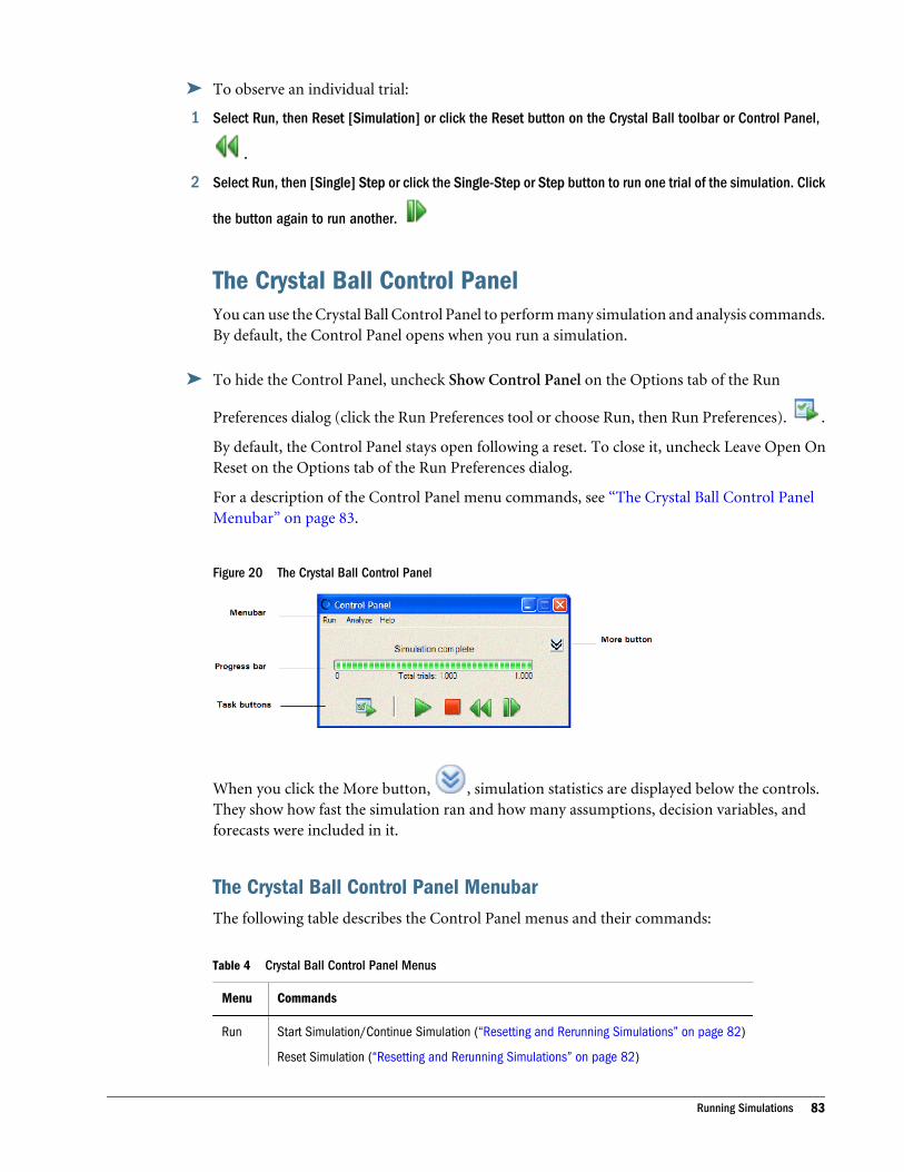
ä To observe an individual trial:
1 Select Run, then Reset [Simulation] or click the Reset button on the Crystal Ball toolbar or Control Panel,
.
2 Select Run, then [Single] Step or click the Single-Step or Step button to run one trial of the simulation. Click
the button again to run another.
The Crystal Ball Control PanelYou can use the Crystal Ball Control Panel to perform many simulation and analysis commands.By default, the Control Panel opens when you run a simulation.
ä To hide the Control Panel, uncheck Show Control Panel on the Options tab of the Run
Preferences dialog (click the Run Preferences tool or choose Run, then Run Preferences). .
By default, the Control Panel stays open following a reset. To close it, uncheck Leave Open OnReset on the Options tab of the Run Preferences dialog.
For a description of the Control Panel menu commands, see “The Crystal Ball Control PanelMenubar” on page 83.
Figure 20 The Crystal Ball Control Panel
When you click the More button, , simulation statistics are displayed below the controls.They show how fast the simulation ran and how many assumptions, decision variables, andforecasts were included in it.
The Crystal Ball Control Panel MenubarThe following table describes the Control Panel menus and their commands:
Table 4 Crystal Ball Control Panel Menus
Menu Commands
Run Start Simulation/Continue Simulation (“Resetting and Rerunning Simulations” on page 82)
Reset Simulation (“Resetting and Rerunning Simulations” on page 82)
Running Simulations 83
Menu Commands
Single Step (“Single-Stepping” on page 82)
OptQuest
Predictor
More Tools (“Overview” on page 167)
Save Results (“Saving Crystal Ball Simulation Results” on page 86)
Restore Results (“Restoring Crystal Ball Simulation Results” on page 87)
Run Preferences (“Setting Run Preferences” on page 76)
Analyze Assumption Charts (“Understanding and Using Assumption Charts” on page 147)
Forecast Charts (“Defining Forecasts” on page 64)
Overlay Charts (“Understanding and Using Overlay Charts” on page 126)
Trend Charts (“Understanding and Using Trend Charts” on page 131)
Sensitivity Charts (“Understanding and Using Sensitivity Charts” on page 138)
Cascade (“Multiple Windows” on page 84)
Close All (“Multiple Windows” on page 84)
Create Report (“Creating Reports” on page 157)
Extract Data (“Extracting Data” on page 161)
Help Control Panel Help
Managing Chart WindowsYou can close the forecast and other chart windows at any time and the simulation will continue.Running a simulation with the windows closed decreases the time required to run the simulation.
The following sections describe how to work with single and multiple chart windows:
l “Single Windows” on page 84
l “Multiple Windows” on page 84
Single WindowsTo close one window, click the Close icon in the upper right corner of the chart window.
Multiple WindowsYou can use several commands on the Analyze menu and Crystal Ball toolbar to:
l Close and cascade all open forecast windows and other chart windows.
l Open charts that have been closed.
l Create new charts.
84 Running Simulations

l Delete overlay, trend, and sensitivity charts.
If you are using Crystal Ball in Excel 2007, choose Analyze, then View Charts and then choosea command.
You can click a chart button (shown below) to open all windows for that chart type, or use oneof the following commands:
l Analyze, then Open Selected Cells (In Excel 2007, choose Analyze, then View Charts, thenOpen From Selection) — Opens charts for all assumption and forecast cells in the selectedrange. [xxx confirm command names; may be the same now]
l Analyze, then Assumption Charts (In Excel 2007, choose Analyze, then View Charts,then Assumption Charts) — Opens a dialog so you can choose which assumption charts toopen or close.
l Analyze, then Forecast Charts (In Excel 2007, choose Analyze, then View Charts, thenForecast Charts) — Opens a dialog so you can choose which forecast charts to open or close.
l Analyze, then Overlay Charts (In Excel 2007, choose Analyze, then View Charts, thenOverlay Charts) — Opens a dialog so you can choose which overlay charts to open or close,create, or delete.
l Analyze, then Trend Charts (In Excel 2007, choose Analyze, then View Charts, thenTrend Charts) — Opens a dialog so you can choose which trend charts to open or close,create, or delete.
l Analyze, then Sensitivity Charts (In Excel 2007, choose Analyze, then View Charts, thenSensitivity Charts) — Opens a dialog so you can choose which sensitivity charts to open orclose, create, or delete.
l Analyze, then Scatter Charts (In Excel 2007, choose Analyze, then View Charts, thenScatter Charts) — Opens a dialog so you can choose which scatter charts to open or close,create, or delete.
l Analyze, then OptQuest Charts (In Excel 2007, choose Analyze, then View Charts,then OptQuest Charts) — If OptQuest is available and you have just run an optimization,opens a dialog so you can choose which OptQuest charts to open or close, create, or delete.
l Analyze, then Predictor Charts (In Excel 2007, choose Analyze, then View Charts, thenPredictor Charts) — If you have just run an time series forecast, opens a dialog so you canchoose which Predictor charts to open or close, create, or delete.
l Analyze, then Close All (In Excel 2007, choose Analyze, then View Charts, then Close All)— Closes all chart windows and clears the current simulation results and stored results frommemory.
l Analyze, then Cascade (In Excel 2007, choose Analyze, then View Charts, then Cascade) —Neatly stacks all windows in front of Excel.
Managing Chart Windows 85
See “Setting Speed Preferences” on page 78 for ways to control whether and how often chartwindows display and redraw.
Saving and Restoring Simulation ResultsYou can save all open forecast windows and other charts as well as simulation data after you runa simulation in Crystal Ball. You can only save results after a simulation stops. Although onlyresults are saved and not an entire model, restored results files are displayed in Crystal Ball chart,report, and Extract Data dialogs so you can work with them. You can run new charts and reportsagainst them and extract their data to worksheets. Only results from the current simulation aresaved.
Because the saved files contain only results and are not complete models, you can load morethan one results file at a time and you do not need to reset the current simulation before loadingresults.
The following sections describe how to save, restore, and work with saved simulation results:
l “Saving Crystal Ball Simulation Results” on page 86
l “Restoring Crystal Ball Simulation Results” on page 87
l “Using Restored Results” on page 87
l “Restored Results with Capability Metrics” on page 87
Saving Crystal Ball Simulation Results
ä To save Crystal Ball results:
1 Choose Run, then Save Results. The Save Results dialog opens.
(In Excel 2007, choose Run, then Save or Restore, and then choose Save Results.)
2 Navigate to the correct folder to save the results file.
3 Name the results file. The default name is the name of the active workbook.
4 Click OK.
The saved results file has a .cbr extension. Crystal Ball saves all results data and charts that existedwhen the results were saved.
Note: Only results from the current simulation are saved. Previously restored results are notsaved. Suppose current and restored forecasts are both used in an overlay chart. If theoverlay chart is then saved as part of the current simulation results, when it is restored itwill only contain forecasts from the saved current results set. Forecasts from the previouslyrestored results will no longer be included in the chart.
86 Running Simulations
Restoring Crystal Ball Simulation Results
ä To restore Crystal Ball simulation results that you saved earlier:
1 Select Run, then Restore Results. If you are using Crystal Ball in Excel 2007, choose Run, then Save orRestore, then Restore Results.
2 When the Restore Results dialog opens, select the results file (.cbr file type) to restore and click Open.
Because you are restoring results and not simulation cell definitions or data, you do not need toreset the simulation before restoring results.
Results files can be restored at any time, regardless of whether the original workbooks are openor whether another simulation has run or not. You can open as many results files as you want— not just one as in Crystal Ball 2000 or earlier versions of Crystal Ball. However, you can onlychoose one at a time in the Restore Results dialog.
Note: If you try to load results from Crystal Ball 7.3 or later into an earlier version of CrystalBall, an error message might be displayed, explaining that the Crystal Ball data containedin the selected result set cannot be loaded. One reason this message might be displayed isthat a new chart type, scatter charts, was added in Crystal Ball 7.3. In this case, it could behelpful to load the entire model, not just saved results. If you load a model containingscatter charts into an earlier version of Crystal Ball, the model will run and the scattercharts will be ignored.
Using Restored ResultsAfter you have restored one or more Crystal Ball results files, you can open and close restoredcharts, create new reports using them, and extract their data to spreadsheets. You can createoverlay and trend charts with restored results and results from the current simulation to comparedata. The results are displayed in dialogs following those for the current simulation.
ä To remove restored results from memory, choose Analyze, then Close All. In Excel 2007, chooseAnalyze, then View Charts, then Close All.
Restored Results with Capability MetricsIf you calculate capability metrics, store the results in a .cbr file, and then restore the results, therestored results use the preference settings on the machine where the results are restored. Thesemight be different from the settings when the original simulation was run and stored. CrystalBall refits the data when the results are restored, so results might differ somewhat from theoriginal results.
Saving and Restoring Simulation Results 87
Functions for Use in Excel ModelsYou can use subroutines and functions in the Crystal Ball Developer Kit to automate certainCrystal Ball operations. The following Crystal Ball functions are available as spreadsheetfunctions for use in Excel models:
l CB.GetAssumFN — Retrieves information for a specific assumption cell.
l CB.GetAssumPercentFN — Returns the value corresponding to a percentile for anassumption cell.
l CB.GetCertaintyFN — Returns the certainty level of achieving a forecast value at or belowa specific threshold.
l CB.GetForeDataFN — Returns the value for the given trial for a specific forecast.
l CB.GetForePercentFN — Returns the value corresponding to a percentile for a specificforecast.
l CB.GetForeStatFN — Returns statistic for a specific forecast cell.
l CB.GetRunPrefsFN — Returns a Run Preference setting.
l CB.IterationsFN — Returns the number of trials run in a simulation.
ä To use these functions with Crystal Ball loaded:
1 Select an empty spreadsheet cell and choose Insert, then Function. In Excel 2007, choose Formulas, thenInsert Function.
2 Select the Crystal Ball category in the category list box.
3 Find the function in the function list. Select it and click OK. Always choose the function ending in FN, sincethe other runs significantly slower in most cases.
4 In the Function Arguments dialog, enter any required arguments and click OK.
The requested value is displayed in the cell with the function.
Running User-Defined MacrosYou can run user-defined Excel VBA macros automatically during a simulation by naming themwith predefined names:
l CBBeforeSimulation — Runs immediately after the Start Simulation command or Single-Step command
l CBBeforeTrial — Runs before random numbers have been placed in assumption cells
l CBAfterRecalc — Runs after Excel has recalculated the model but before a trial value hasbeen retrieved from the forecast cells
l CBAfterTrial — Runs after the forecast trial values have been retrieved and entered into theforecast charts
l CBAfterSimulation — Runs when the simulation is complete or stopped with a Stopcommand, by single-stepping (after each step), or for any other reason
88 Running Simulations
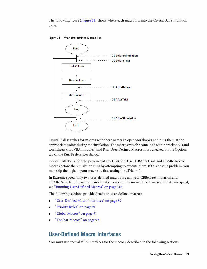
The following figure (Figure 21) shows where each macro fits into the Crystal Ball simulationcycle.
Figure 21 When User-Defined Macros Run
Crystal Ball searches for macros with these names in open workbooks and runs them at theappropriate points during the simulation. The macros must be contained within workbooks andworksheets (not VBA modules) and Run User-Defined Macros must checked on the Optionstab of the Run Preferences dialog.
Crystal Ball checks for the presence of any CBBeforeTrial, CBAfterTrial, and CBAfterRecalcmacros before the simulation runs by attempting to execute them. If this poses a problem, youmay skip the logic in your macro by first testing for aTrial = 0.
In Extreme speed, only two user-defined macros are allowed: CBBeforeSimulation andCBAfterSimulation. For more information on running user-defined macros in Extreme speed,see “Running User-Defined Macros” on page 316.
The following sections provide details on user-defined macros:
l “User-Defined Macro Interfaces” on page 89
l “Priority Rules” on page 91
l “Global Macros” on page 91
l “Toolbar Macros” on page 92
User-Defined Macro InterfacesYou must use special VBA interfaces for the macros, described in the following sections:
Running User-Defined Macros 89
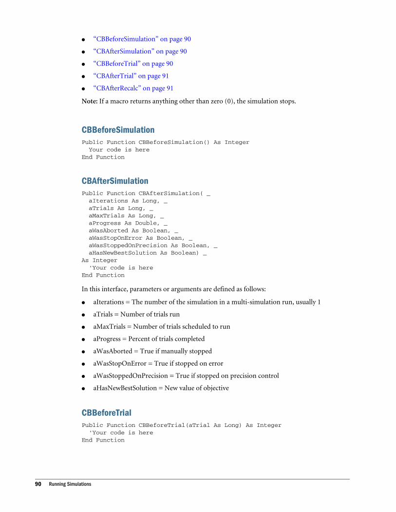
l “CBBeforeSimulation” on page 90
l “CBAfterSimulation” on page 90
l “CBBeforeTrial” on page 90
l “CBAfterTrial” on page 91
l “CBAfterRecalc” on page 91
Note: If a macro returns anything other than zero (0), the simulation stops.
CBBeforeSimulationPublic Function CBBeforeSimulation() As Integer Your code is hereEnd Function
CBAfterSimulationPublic Function CBAfterSimulation( _ aIterations As Long, _ aTrials As Long, _ aMaxTrials As Long, _ aProgress As Double, _ aWasAborted As Boolean, _ aWasStopOnError As Boolean, _ aWasStoppedOnPrecision As Boolean, _ aHasNewBestSolution As Boolean) _As Integer 'Your code is hereEnd Function
In this interface, parameters or arguments are defined as follows:
l aIterations = The number of the simulation in a multi-simulation run, usually 1
l aTrials = Number of trials run
l aMaxTrials = Number of trials scheduled to run
l aProgress = Percent of trials completed
l aWasAborted = True if manually stopped
l aWasStopOnError = True if stopped on error
l aWasStoppedOnPrecision = True if stopped on precision control
l aHasNewBestSolution = New value of objective
CBBeforeTrialPublic Function CBBeforeTrial(aTrial As Long) As Integer 'Your code is hereEnd Function
90 Running Simulations
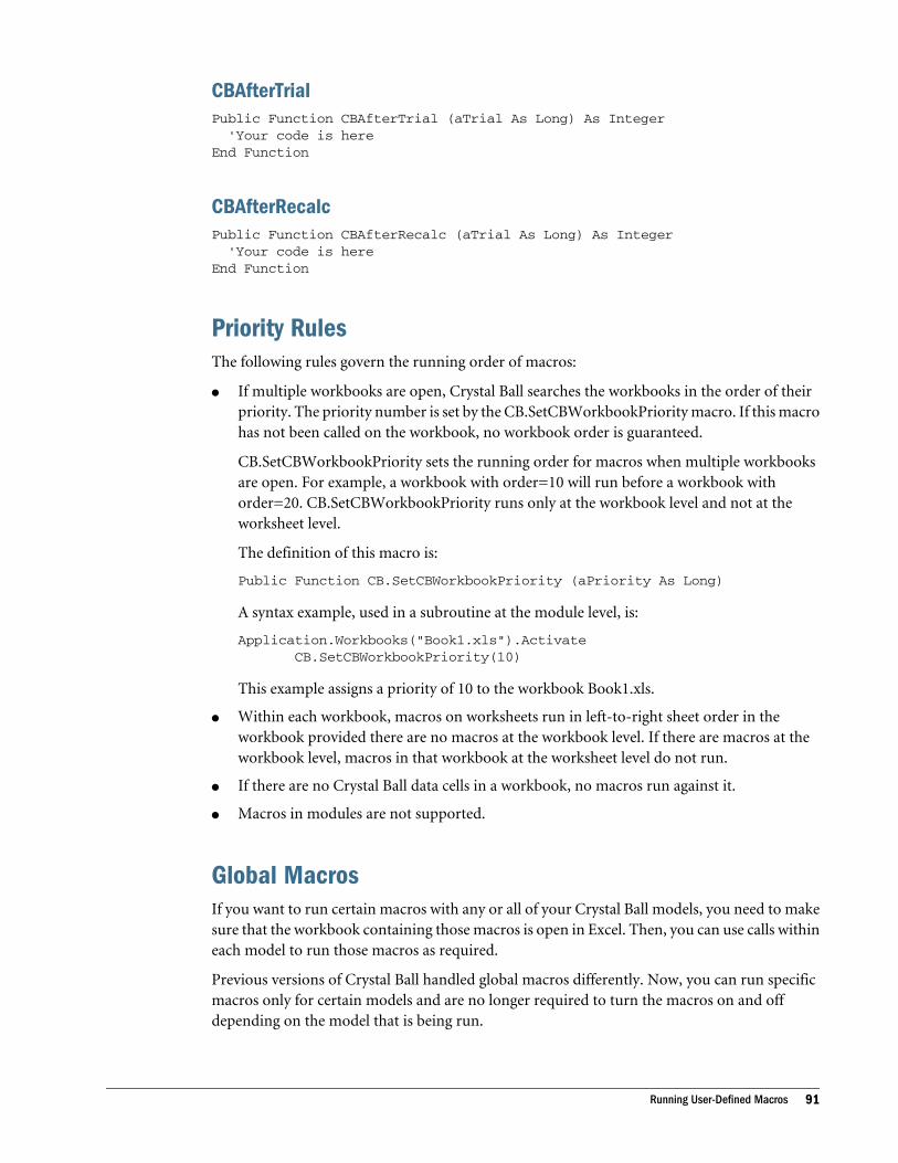
CBAfterTrialPublic Function CBAfterTrial (aTrial As Long) As Integer 'Your code is hereEnd Function
CBAfterRecalcPublic Function CBAfterRecalc (aTrial As Long) As Integer 'Your code is hereEnd Function
Priority RulesThe following rules govern the running order of macros:
l If multiple workbooks are open, Crystal Ball searches the workbooks in the order of theirpriority. The priority number is set by the CB.SetCBWorkbookPriority macro. If this macrohas not been called on the workbook, no workbook order is guaranteed.
CB.SetCBWorkbookPriority sets the running order for macros when multiple workbooksare open. For example, a workbook with order=10 will run before a workbook withorder=20. CB.SetCBWorkbookPriority runs only at the workbook level and not at theworksheet level.
The definition of this macro is:
Public Function CB.SetCBWorkbookPriority (aPriority As Long)
A syntax example, used in a subroutine at the module level, is:
Application.Workbooks("Book1.xls").Activate CB.SetCBWorkbookPriority(10)
This example assigns a priority of 10 to the workbook Book1.xls.
l Within each workbook, macros on worksheets run in left-to-right sheet order in theworkbook provided there are no macros at the workbook level. If there are macros at theworkbook level, macros in that workbook at the worksheet level do not run.
l If there are no Crystal Ball data cells in a workbook, no macros run against it.
l Macros in modules are not supported.
Global MacrosIf you want to run certain macros with any or all of your Crystal Ball models, you need to makesure that the workbook containing those macros is open in Excel. Then, you can use calls withineach model to run those macros as required.
Previous versions of Crystal Ball handled global macros differently. Now, you can run specificmacros only for certain models and are no longer required to turn the macros on and offdepending on the model that is being run.
Running User-Defined Macros 91

Toolbar MacrosIf you want to use custom Excel toolbar macros defined in a separate workbook while CrystalBall is loaded, be sure to save that workbook to the folder C:\Documents and Settings\yourname\Application Data\Microsoft\Excel\XLSTART.
92 Running Simulations
6Analyzing Forecast Charts
In This Chapter
Introduction... . . . . . . . . . . . . . . . . . . . . . . . . . . . . . . . . . . . . . . . . . . . . . . . . . . . . . . . . . . . . . . . . . . . . . . . . . . . . . . . . . . . . . . . . . . . . . . . . . . . . . . . . . . . . . . . . . . . . . .93
Guidelines for Analyzing Simulation Results.. . . . . . . . . . . . . . . . . . . . . . . . . . . . . . . . . . . . . . . . . . . . . . . . . . . . . . . . . . . . . . . . . . . . . . . . . . . . . . . . . . . .93
Understanding and Using Forecast Charts.. . . . . . . . . . . . . . . . . . . . . . . . . . . . . . . . . . . . . . . . . . . . . . . . . . . . . . . . . . . . . . . . . . . . . . . . . . . . . . . . . . . . . .95
Setting Chart Preferences ... . . . . . . . . . . . . . . . . . . . . . . . . . . . . . . . . . . . . . . . . . . . . . . . . . . . . . . . . . . . . . . . . . . . . . . . . . . . . . . . . . . . . . . . . . . . . . . . . . . . . 112
Managing Existing Charts.. . . . . . . . . . . . . . . . . . . . . . . . . . . . . . . . . . . . . . . . . . . . . . . . . . . . . . . . . . . . . . . . . . . . . . . . . . . . . . . . . . . . . . . . . . . . . . . . . . . . . . . 121
IntroductionThis chapter describes how to use forecast charts to analyze simulation results. As you readthrough the chapter, you will learn to focus on a particular range of simulation results, analyzeforecast charts, and interpret relevant descriptive statistics.
You will also learn how to customize forecast charts, work with chart windows, and share chartswith other applications.
Chapter 7 introduces additional charts. Chapter 8 describes how to extract Crystal Ballsimulation data for use in Excel and other applications and how to prepare reports.
Guidelines for Analyzing Simulation ResultsWhile a simulation runs, Crystal Ball creates a forecast chart for each forecast cell. Forecast chartscondense much information into a small space. You can display that information in severaldifferent ways, both graphically and numerically.
When you analyze a simulation, you can focus on forecast charts. You can also display otherkinds of charts, generate reports, and extract data for further processing using Excel or otheranalysis tools.
The following steps can help guide your simulation analysis by focusing on details as well asgeneral trends:
1. Look at the "big picture."
Consider each forecast chart from a high-level viewpoint. Look at the shape of thedistribution:
l Is it distributed normally or skewed negatively or positively?
Introduction 93
l Is it "flat" (spread out on both sides of the mean) or "peaked" (with most values clusteredclosely around the mean)?
l Does it have a single mode (most likely value) or is it bimodal with several "peaks" or"humps"?
l Is it continuous or are there groups of values separated from the rest, maybe evenextreme "outliers" that fall outside of the display range?
The statistical concepts in the "Statistical Definitions" chapter of the online OracleCrystal Ball Statistical Guide can help with this part of your analysis.
2. Look at the certainty level, the probability of achieving values within a certain range.
You can enter a range, such as all values greater than $0 dollars if you’re analyzing profits,and view the certainty of falling within the range ($0 to + Infinity, in this case). You can alsoenter a certainty, say 75%, and see what range of values would be required to meet that level.“Determining the Certainty Level” on page 96 explains these and other ways of analyzingcertainty.
3. Focus on the display range.
You can change the display range to focus on different sections of the forecast chart. Forexample, you can set the display range to focus on just the upper or lower tail of the forecast.“Focusing On the Display Range” on page 100 discusses this analysis technique.
4. Look at different views of the forecast.
Use the View menu to switch among different ways of viewing the forecast distributiongraphically (frequency, cumulative frequency, or reverse cumulative frequency) ornumerically (statistics, percentiles, goodness of fit data, or capability metrics). You can alsochoose whether to show charts and statistics simultaneously or separately. For instructions,see “Changing the Distribution View and Interpreting Statistics” on page 102.
5. Customize the forecast chart.
Use the chart preferences to change graphic presentations from bars to areas or lines, orexperiment with different colors, 2D versus 3D, more or fewer plotted intervals or datapoints, and other display variations. “Setting Chart Preferences” on page 112 describes themany ways you can format charts for analysis and presentation of results.
6. Create other kinds of charts.
You can display overlay charts (“Understanding and Using Overlay Charts” on page 126),trend charts (“Understanding and Using Trend Charts” on page 131), sensitivity charts(“Understanding and Using Sensitivity Charts” on page 138), assumption charts(“Understanding and Using Assumption Charts” on page 147), and scatter charts(“Understanding and Using Scatter Charts” on page 149). As with forecast charts, you cancustomize these charts as well. Selecting different views of the data can help you analyze itand present it to others.
7. Create reports.
Create reports with charts and data (“Creating Reports” on page 157). You can quicklyproduce pre-defined or custom reports for analysis and presentation.
8. Extract data for numeric analysis and presentation.
94 Analyzing Forecast Charts
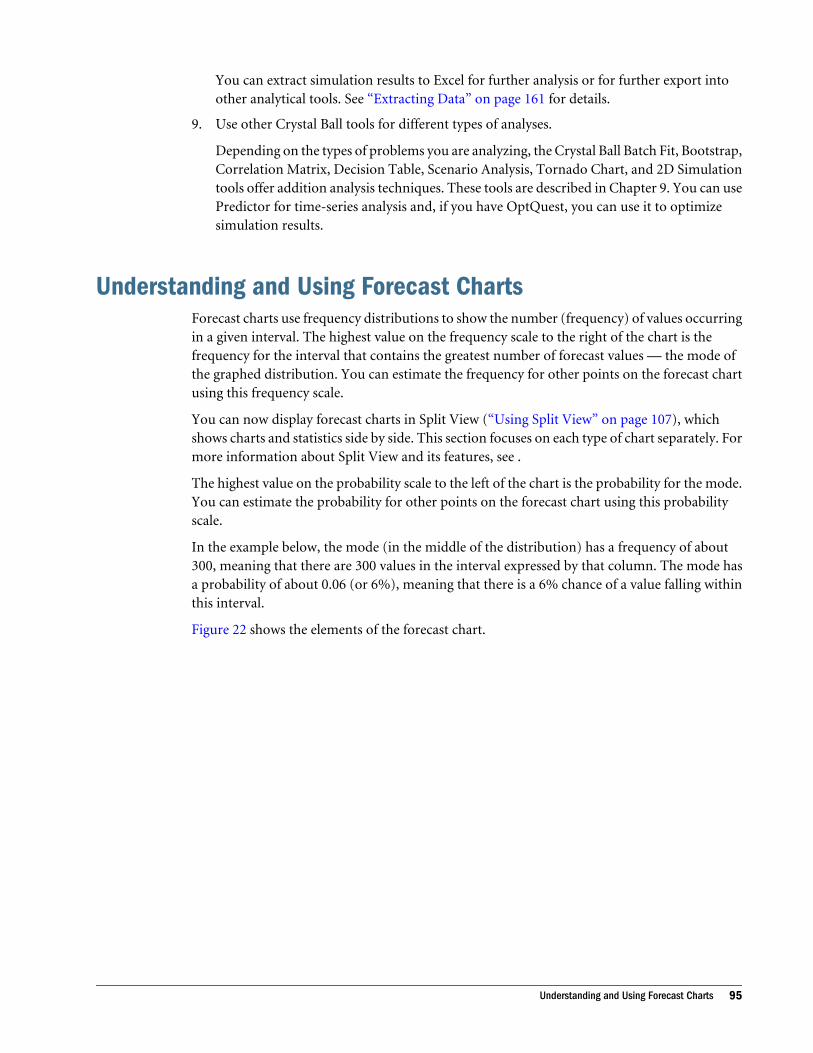
You can extract simulation results to Excel for further analysis or for further export intoother analytical tools. See “Extracting Data” on page 161 for details.
9. Use other Crystal Ball tools for different types of analyses.
Depending on the types of problems you are analyzing, the Crystal Ball Batch Fit, Bootstrap,Correlation Matrix, Decision Table, Scenario Analysis, Tornado Chart, and 2D Simulationtools offer addition analysis techniques. These tools are described in Chapter 9. You can usePredictor for time-series analysis and, if you have OptQuest, you can use it to optimizesimulation results.
Understanding and Using Forecast ChartsForecast charts use frequency distributions to show the number (frequency) of values occurringin a given interval. The highest value on the frequency scale to the right of the chart is thefrequency for the interval that contains the greatest number of forecast values — the mode ofthe graphed distribution. You can estimate the frequency for other points on the forecast chartusing this frequency scale.
You can now display forecast charts in Split View (“Using Split View” on page 107), whichshows charts and statistics side by side. This section focuses on each type of chart separately. Formore information about Split View and its features, see .
The highest value on the probability scale to the left of the chart is the probability for the mode.You can estimate the probability for other points on the forecast chart using this probabilityscale.
In the example below, the mode (in the middle of the distribution) has a frequency of about300, meaning that there are 300 values in the interval expressed by that column. The mode hasa probability of about 0.06 (or 6%), meaning that there is a 6% chance of a value falling withinthis interval.
Figure 22 shows the elements of the forecast chart.
Understanding and Using Forecast Charts 95
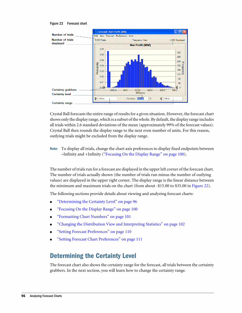
Figure 22 Forecast chart
Crystal Ball forecasts the entire range of results for a given situation. However, the forecast chartshows only the display range, which is a subset of the whole. By default, the display range includesall trials within 2.6 standard deviations of the mean (approximately 99% of the forecast values).Crystal Ball then rounds the display range to the next even number of units. For this reason,outlying trials might be excluded from the display range.
Note: To display all trials, change the chart axis preferences to display fixed endpoints between–Infinity and +Infinity (“Focusing On the Display Range” on page 100).
The number of trials run for a forecast are displayed in the upper left corner of the forecast chart.The number of trials actually shown (the number of trials run minus the number of outlyingvalues) are displayed in the upper right corner. The display range is the linear distance betweenthe minimum and maximum trials on the chart (from about -$15.00 to $35.00 in Figure 22).
The following sections provide details about viewing and analyzing forecast charts:
l “Determining the Certainty Level” on page 96
l “Focusing On the Display Range” on page 100
l “Formatting Chart Numbers” on page 101
l “Changing the Distribution View and Interpreting Statistics” on page 102
l “Setting Forecast Preferences” on page 110
l “Setting Forecast Chart Preferences” on page 111
Determining the Certainty LevelThe forecast chart also shows the certainty range for the forecast, all trials between the certaintygrabbers. In the next section, you will learn how to change the certainty range.
96 Analyzing Forecast Charts
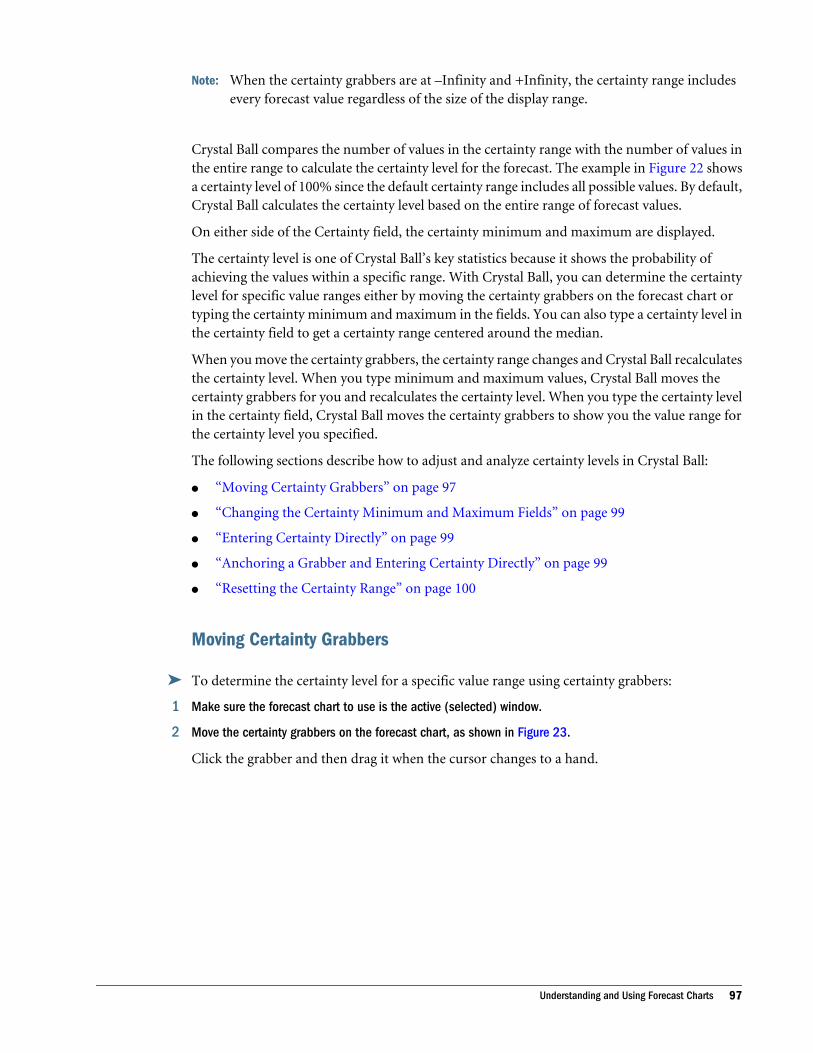
Note: When the certainty grabbers are at –Infinity and +Infinity, the certainty range includesevery forecast value regardless of the size of the display range.
Crystal Ball compares the number of values in the certainty range with the number of values inthe entire range to calculate the certainty level for the forecast. The example in Figure 22 showsa certainty level of 100% since the default certainty range includes all possible values. By default,Crystal Ball calculates the certainty level based on the entire range of forecast values.
On either side of the Certainty field, the certainty minimum and maximum are displayed.
The certainty level is one of Crystal Ball’s key statistics because it shows the probability ofachieving the values within a specific range. With Crystal Ball, you can determine the certaintylevel for specific value ranges either by moving the certainty grabbers on the forecast chart ortyping the certainty minimum and maximum in the fields. You can also type a certainty level inthe certainty field to get a certainty range centered around the median.
When you move the certainty grabbers, the certainty range changes and Crystal Ball recalculatesthe certainty level. When you type minimum and maximum values, Crystal Ball moves thecertainty grabbers for you and recalculates the certainty level. When you type the certainty levelin the certainty field, Crystal Ball moves the certainty grabbers to show you the value range forthe certainty level you specified.
The following sections describe how to adjust and analyze certainty levels in Crystal Ball:
l “Moving Certainty Grabbers” on page 97
l “Changing the Certainty Minimum and Maximum Fields” on page 99
l “Entering Certainty Directly” on page 99
l “Anchoring a Grabber and Entering Certainty Directly” on page 99
l “Resetting the Certainty Range” on page 100
Moving Certainty Grabbers
ä To determine the certainty level for a specific value range using certainty grabbers:
1 Make sure the forecast chart to use is the active (selected) window.
2 Move the certainty grabbers on the forecast chart, as shown in Figure 23.
Click the grabber and then drag it when the cursor changes to a hand.
Understanding and Using Forecast Charts 97
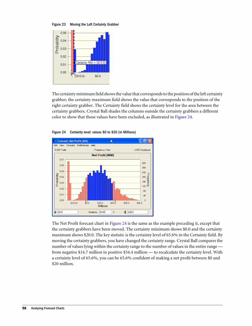
Figure 23 Moving the Left Certainty Grabber
The certainty minimum field shows the value that corresponds to the position of the left certaintygrabber; the certainty maximum field shows the value that corresponds to the position of theright certainty grabber. The Certainty field shows the certainty level for the area between thecertainty grabbers. Crystal Ball shades the columns outside the certainty grabbers a differentcolor to show that those values have been excluded, as illustrated in Figure 24.
Figure 24 Certainty level: values $0 to $20 (in Millions)
The Net Profit forecast chart in Figure 24 is the same as the example preceding it, except thatthe certainty grabbers have been moved. The certainty minimum shows $0.0 and the certaintymaximum shows $20.0. The key statistic is the certainty level of 65.6% in the Certainty field. Bymoving the certainty grabbers, you have changed the certainty range. Crystal Ball compares thenumber of values lying within the certainty range to the number of values in the entire range —from negative $14.7 million to positive $34.4 million — to recalculate the certainty level. Witha certainty level of 65.6%, you can be 65.6% confident of making a net profit between $0 and$20 million.
98 Analyzing Forecast Charts
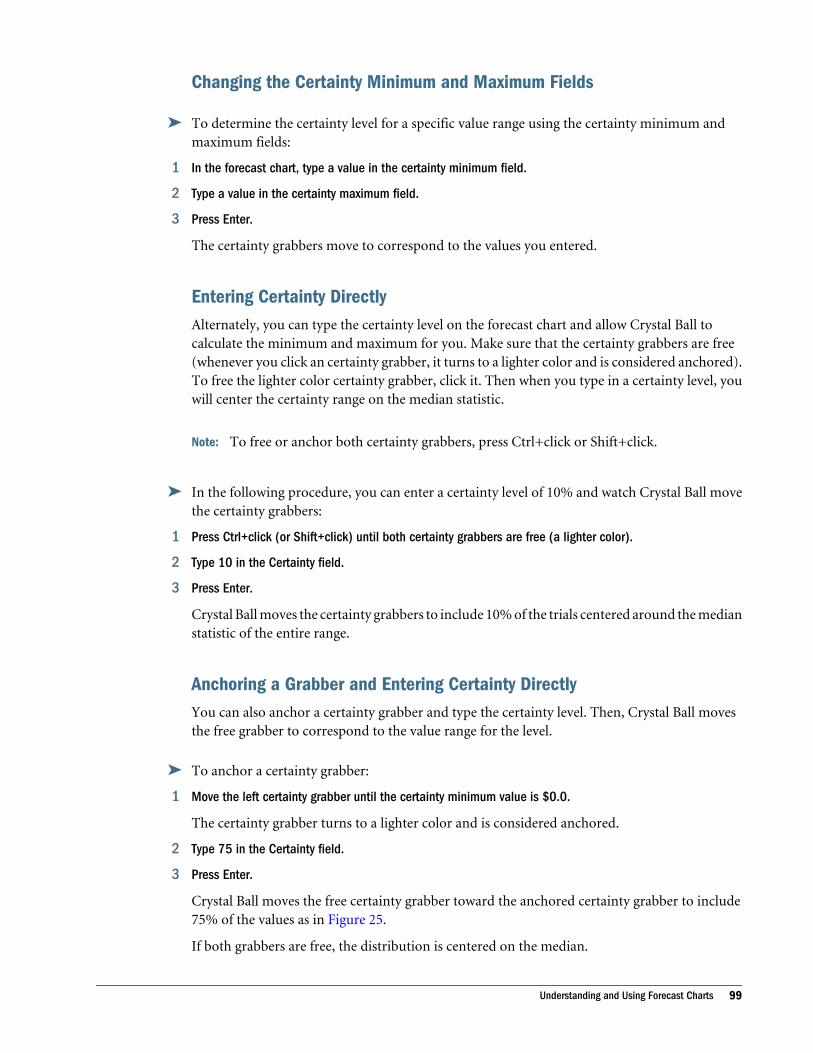
Changing the Certainty Minimum and Maximum Fields
ä To determine the certainty level for a specific value range using the certainty minimum andmaximum fields:
1 In the forecast chart, type a value in the certainty minimum field.
2 Type a value in the certainty maximum field.
3 Press Enter.
The certainty grabbers move to correspond to the values you entered.
Entering Certainty DirectlyAlternately, you can type the certainty level on the forecast chart and allow Crystal Ball tocalculate the minimum and maximum for you. Make sure that the certainty grabbers are free(whenever you click an certainty grabber, it turns to a lighter color and is considered anchored).To free the lighter color certainty grabber, click it. Then when you type in a certainty level, youwill center the certainty range on the median statistic.
Note: To free or anchor both certainty grabbers, press Ctrl+click or Shift+click.
ä In the following procedure, you can enter a certainty level of 10% and watch Crystal Ball movethe certainty grabbers:
1 Press Ctrl+click (or Shift+click) until both certainty grabbers are free (a lighter color).
2 Type 10 in the Certainty field.
3 Press Enter.
Crystal Ball moves the certainty grabbers to include 10% of the trials centered around the medianstatistic of the entire range.
Anchoring a Grabber and Entering Certainty DirectlyYou can also anchor a certainty grabber and type the certainty level. Then, Crystal Ball movesthe free grabber to correspond to the value range for the level.
ä To anchor a certainty grabber:
1 Move the left certainty grabber until the certainty minimum value is $0.0.
The certainty grabber turns to a lighter color and is considered anchored.
2 Type 75 in the Certainty field.
3 Press Enter.
Crystal Ball moves the free certainty grabber toward the anchored certainty grabber to include75% of the values as in Figure 25.
If both grabbers are free, the distribution is centered on the median.
Understanding and Using Forecast Charts 99
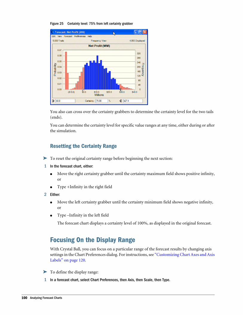
Figure 25 Certainty level: 75% from left certainty grabber
You also can cross over the certainty grabbers to determine the certainty level for the two tails(ends).
You can determine the certainty level for specific value ranges at any time, either during or afterthe simulation.
Resetting the Certainty Range
ä To reset the original certainty range before beginning the next section:
1 In the forecast chart, either:
l Move the right certainty grabber until the certainty maximum field shows positive infinity,or
l Type +Infinity in the right field
2 Either:
l Move the left certainty grabber until the certainty minimum field shows negative infinity,or
l Type –Infinity in the left field
The forecast chart displays a certainty level of 100%, as displayed in the original forecast.
Focusing On the Display RangeWith Crystal Ball, you can focus on a particular range of the forecast results by changing axissettings in the Chart Preferences dialog. For instructions, see “Customizing Chart Axes and AxisLabels” on page 120.
ä To define the display range:
1 In a forecast chart, select Chart Preferences, then Axis, then Scale, then Type.
100 Analyzing Forecast Charts
2 Choose a scale type:
l Auto — Crystal Ball uses a default display range of 2.6 standard deviations from the mean,which includes about 99% of the forecast values. (See Standard Deviation, following.)
l Fixed — Sets the display range end points manually so you can focus on particular valueranges. For example, you can focus on positive values only to look at the profit for a profit/loss forecast.
l Standard Deviation — Sets the display range end points in terms of standard deviations;defines the number of standard deviations worth of value to display on each side of the meanand centers values around the mean. If you choose to set the display range in terms ofstandard deviations, you can change the display range to 1 standard deviation from the meanto look at approximately 68% of the forecast values.
l Percentile — Sets the display range end points in terms of percentiles.
By default, the x-axis value numbers are automatically adjusted to round numbers to makethe forecasts easier to read. The Axis chart preference settings include Round Display Range,which constrains the display range to round numbers. You can uncheck this setting to displayactual, unrounded numbers.
Other chart customizations are available to help you interpret the results of the simulation byviewing the data in different ways. For details, see “Setting Chart Preferences” on page 112.
Also see “Setting Preferences with Shortcut Keys” on page 112 for ways to change the appearanceof charts without using menu commands.
Showing Statistics for the Display RangeAfter you have changed the display range, you can display statistics for just that range.
ä To show statistics for a display range:
1 Set the display range as described in “Focusing On the Display Range” on page 100.
2 Note the values for the display range minimum and maximum.
3 In the forecast chart menubar, choose Preferences, then Forecast, then Filter.
4 On the Filter tab of the Forecast Preferences dialog, set a filter on the forecast values and include values inthe range between the display range minimum and maximum.
5 When the settings are complete, click OK.
6 Choose View, then Statistics in the forecast chart menubar to show statistics for the display range (or, inSplit View, look at the statistics table on the right side).
Formatting Chart NumbersBy default, the number format displayed on the forecast chart comes from the underlying formatof the forecast cell. You can select another cell format using the Chart Preferences dialog.
Understanding and Using Forecast Charts 101
ä To change the format of numbers in a forecast chart:
1 In the forecast window, choose Preferences, then Chart.
The Chart Preferences dialog opens.
2 Click the Axis tab.
Find the Format Number group.
3 Choose a format from the drop-down list. Available formats are similar to Excel formats. For most formats,you can specify the number of decimal places and whether to use a thousands separator.
4 Click OK to apply the settings, or use Apply To as described in “Applying Settings to the Current Chart andOther Charts” on page 120.
Changing the Distribution View and Interpreting StatisticsThe forecast settings related to distribution type determine the overall appearance of a forecastchart. You can also choose to display a table of statistics or percentiles instead of or in additionto a chart.
ä To set the distribution type or display a data table:
1 Open the View menu in the forecast window.
2 Choose a distribution type or other view to display on the forecast chart:
l Frequency — Shows the number or frequency of values occurring in a given interval. Thisis the default distribution type.
l Cumulative Frequency — Shows the number or proportion (percentage) of values less thanor equal to a given amount.
l Reverse Cumulative Frequency — Shows the number or proportion (percentage) of valuesgreater than or equal to a given amount.
l Statistics — Shows a full set of descriptive statistics for a simulation in the forecast window.
l Percentiles — Shows percentile information in 10% increments, where a percentile is thepercent chance, or probability, of a forecast value being less than or equal to the value thatcorresponds to the percentile (by default).
l Goodness Of Fit — If distribution fitting is selected in the Forecast or Preferences, thenForecast menus, shows goodness-of-fit statistics for the selected distributions and rankingmethods.
l Capability Metrics — If process capability metrics are set for display, shows a table of processcapability (quality) statistics for the simulation (“Viewing Capability Metrics” on page388).
l Split View — Shows all selected views simultaneously (“Using Split View” on page 107).
See “View Examples” on page 103 for descriptions and illustrations of each view.
102 Analyzing Forecast Charts
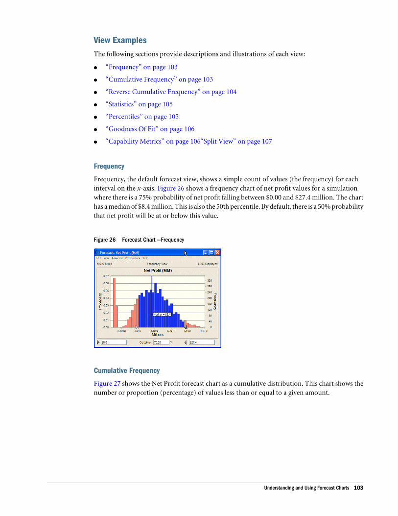
View ExamplesThe following sections provide descriptions and illustrations of each view:
l “Frequency” on page 103
l “Cumulative Frequency” on page 103
l “Reverse Cumulative Frequency” on page 104
l “Statistics” on page 105
l “Percentiles” on page 105
l “Goodness Of Fit” on page 106
l “Capability Metrics” on page 106“Split View” on page 107
Frequency
Frequency, the default forecast view, shows a simple count of values (the frequency) for eachinterval on the x-axis. Figure 26 shows a frequency chart of net profit values for a simulationwhere there is a 75% probability of net profit falling between $0.00 and $27.4 million. The charthas a median of $8.4 million. This is also the 50th percentile. By default, there is a 50% probabilitythat net profit will be at or below this value.
Figure 26 Forecast Chart —Frequency
Cumulative Frequency
Figure 27 shows the Net Profit forecast chart as a cumulative distribution. This chart shows thenumber or proportion (percentage) of values less than or equal to a given amount.
Understanding and Using Forecast Charts 103
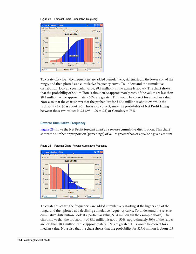
Figure 27 Forecast Chart—Cumulative Frequency
To create this chart, the frequencies are added cumulatively, starting from the lower end of therange, and then plotted as a cumulative frequency curve. To understand the cumulativedistribution, look at a particular value, $8.4 million (in the example above). The chart showsthat the probability of $8.4 million is about 50%; approximately 50% of the values are less than$8.4 million, while approximately 50% are greater. This would be correct for a median value.Note also that the chart shows that the probability for $27.4 million is about .95 while theprobability for $0 is about .20. This is also correct, since the probability of Net Profit fallingbetween those two values is .75 (.95 – .20 = .75) or Certainty = 75%.
Reverse Cumulative Frequency
Figure 28 shows the Net Profit forecast chart as a reverse cumulative distribution. This chartshows the number or proportion (percentage) of values greater than or equal to a given amount.
Figure 28 Forecast Chart—Reverse Cumulative Frequency
To create this chart, the frequencies are added cumulatively starting at the higher end of therange, and then plotted as a declining cumulative frequency curve. To understand the reversecumulative distribution, look at a particular value, $8.4 million (in the example above). Thechart shows that the probability of $8.4 million is about 50%; approximately 50% of the valuesare less than $8.4 million, while approximately 50% are greater. This would be correct for amedian value. Note also that the chart shows that the probability for $27.4 million is about .05
104 Analyzing Forecast Charts
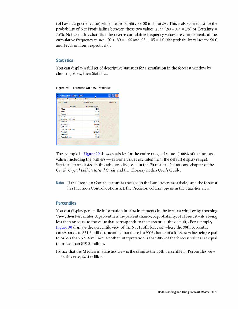
(of having a greater value) while the probability for $0 is about .80. This is also correct, since theprobability of Net Profit falling between those two values is .75 (.80 – .05 = .75) or Certainty =75%. Notice in this chart that the reverse cumulative frequency values are complements of thecumulative frequency values: .20 + .80 = 1.00 and .95 + .05 = 1.0 (the probability values for $0.0and $27.4 million, respectively).
Statistics
You can display a full set of descriptive statistics for a simulation in the forecast window bychoosing View, then Statistics.
Figure 29 Forecast Window—Statistics
The example in Figure 29 shows statistics for the entire range of values (100% of the forecastvalues, including the outliers — extreme values excluded from the default display range).Statistical terms listed in this table are discussed in the "Statistical Definitions" chapter of theOracle Crystal Ball Statistical Guide and the Glossary in this User's Guide.
Note: If the Precision Control feature is checked in the Run Preferences dialog and the forecasthas Precision Control options set, the Precision column opens in the Statistics view.
Percentiles
You can display percentile information in 10% increments in the forecast window by choosingView, then Percentiles. A percentile is the percent chance, or probability, of a forecast value beingless than or equal to the value that corresponds to the percentile (the default). For example,Figure 30 displays the percentile view of the Net Profit forecast, where the 90th percentilecorresponds to $21.6 million, meaning that there is a 90% chance of a forecast value being equalto or less than $21.6 million. Another interpretation is that 90% of the forecast values are equalto or less than $19.3 million.
Notice that the Median in Statistics view is the same as the 50th percentile in Percentiles view— in this case, $8.4 million.
Understanding and Using Forecast Charts 105
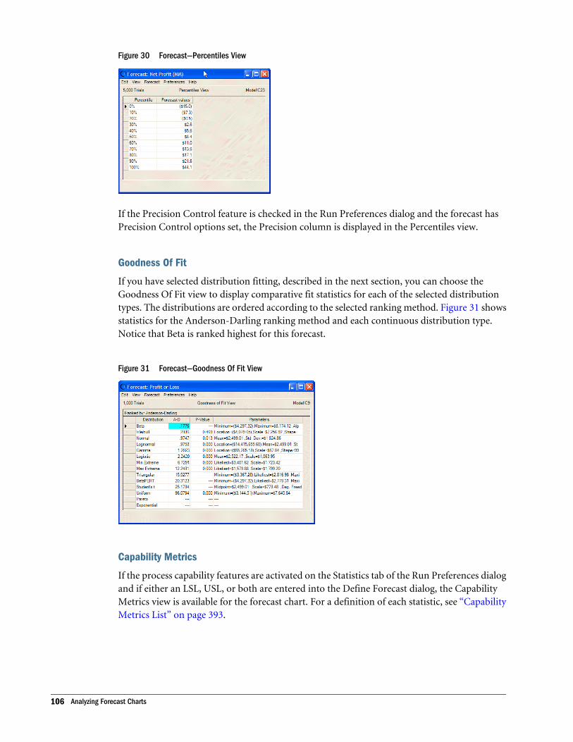
Figure 30 Forecast—Percentiles View
If the Precision Control feature is checked in the Run Preferences dialog and the forecast hasPrecision Control options set, the Precision column is displayed in the Percentiles view.
Goodness Of Fit
If you have selected distribution fitting, described in the next section, you can choose theGoodness Of Fit view to display comparative fit statistics for each of the selected distributiontypes. The distributions are ordered according to the selected ranking method. Figure 31 showsstatistics for the Anderson-Darling ranking method and each continuous distribution type.Notice that Beta is ranked highest for this forecast.
Figure 31 Forecast—Goodness Of Fit View
Capability Metrics
If the process capability features are activated on the Statistics tab of the Run Preferences dialogand if either an LSL, USL, or both are entered into the Define Forecast dialog, the CapabilityMetrics view is available for the forecast chart. For a definition of each statistic, see “CapabilityMetrics List” on page 393.
106 Analyzing Forecast Charts
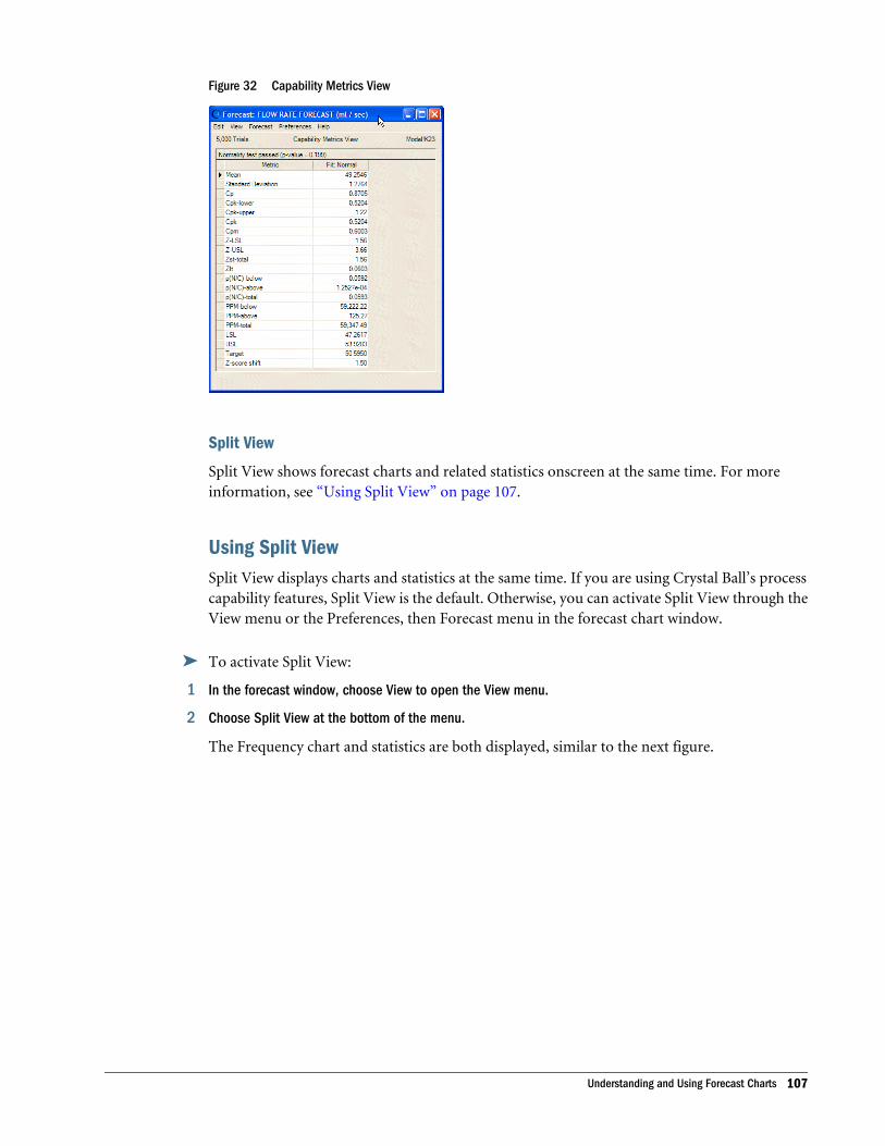
Figure 32 Capability Metrics View
Split View
Split View shows forecast charts and related statistics onscreen at the same time. For moreinformation, see “Using Split View” on page 107.
Using Split ViewSplit View displays charts and statistics at the same time. If you are using Crystal Ball’s processcapability features, Split View is the default. Otherwise, you can activate Split View through theView menu or the Preferences, then Forecast menu in the forecast chart window.
ä To activate Split View:
1 In the forecast window, choose View to open the View menu.
2 Choose Split View at the bottom of the menu.
The Frequency chart and statistics are both displayed, similar to the next figure.
Understanding and Using Forecast Charts 107
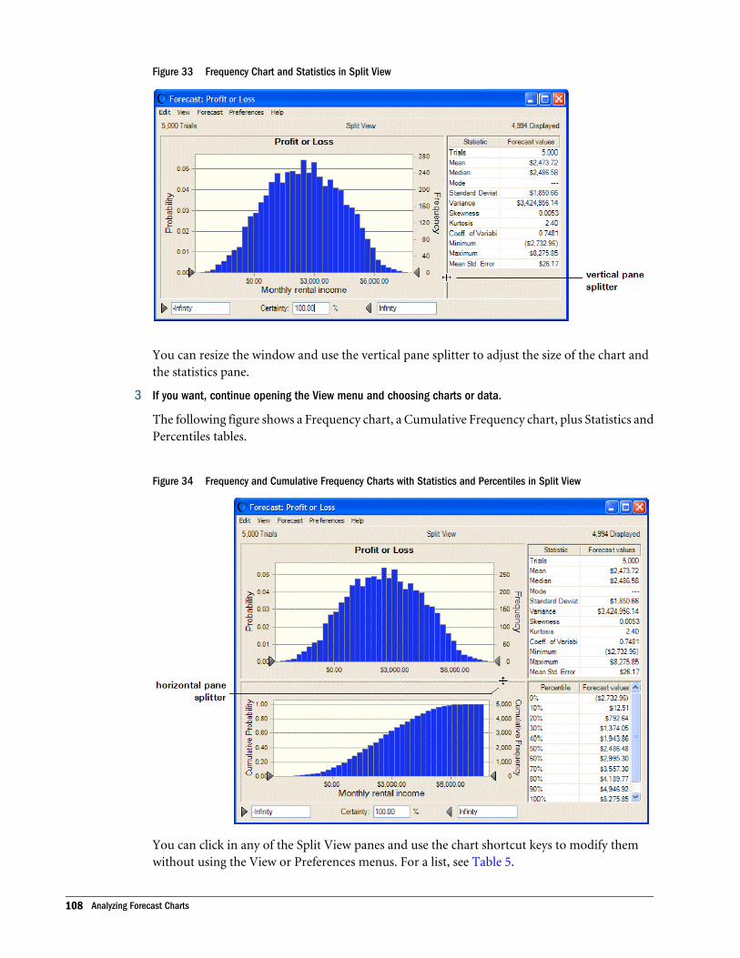
Figure 33 Frequency Chart and Statistics in Split View
You can resize the window and use the vertical pane splitter to adjust the size of the chart andthe statistics pane.
3 If you want, continue opening the View menu and choosing charts or data.
The following figure shows a Frequency chart, a Cumulative Frequency chart, plus Statistics andPercentiles tables.
Figure 34 Frequency and Cumulative Frequency Charts with Statistics and Percentiles in Split View
You can click in any of the Split View panes and use the chart shortcut keys to modify themwithout using the View or Preferences menus. For a list, see Table 5.
108 Analyzing Forecast Charts
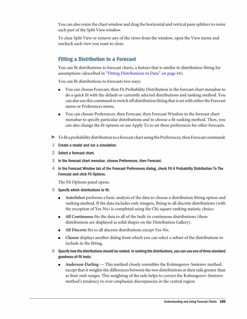
You can also resize the chart window and drag the horizontal and vertical pane splitters to resizeeach part of the Split View window.
To clear Split View or remove any of the views from the window, open the View menu anduncheck each view you want to close.
Fitting a Distribution to a ForecastYou can fit distributions to forecast charts, a feature that is similar to distribution fitting forassumptions (described in “Fitting Distributions to Data” on page 44).
You can fit distributions to forecasts two ways:
l You can choose Forecast, then Fit Probability Distribution in the forecast chart menubar todo a quick fit with the default or currently selected distributions and ranking method. Youcan also use this command to switch off distribution fitting that is set with either the Forecastmenu or Preferences menu.
l You can choose Preferences, then Forecast, then Forecast Window in the forecast chartmenubar to specify particular distributions and to choose a fit ranking method. Then, youcan also change the fit options or use Apply To to set these preferences for other forecasts.
ä To fit a probability distribution to a forecast chart using the Preferences, then Forecast command:
1 Create a model and run a simulation.
2 Select a forecast chart.
3 In the forecast chart menubar, choose Preferences, then Forecast.
4 In the Forecast Window tab of the Forecast Preferences dialog, check Fit A Probability Distribution To TheForecast and click Fit Options.
The Fit Options panel opens.
5 Specify which distributions to fit:
l AutoSelect performs a basic analysis of the data to choose a distribution fitting option andranking method. If the data includes only integers, fitting to all discrete distributions (withthe exception of Yes-No) is completed using the Chi-square ranking statistic choice.
l All Continuous fits the data to all of the built-in continuous distributions (thesedistributions are displayed as solid shapes on the Distribution Gallery).
l All Discrete fits to all discrete distributions except Yes-No.
l Choose displays another dialog from which you can select a subset of the distributions toinclude in the fitting.
6 Specify how the distributions should be ranked. In ranking the distributions, you can use one of three standardgoodness-of-fit tests:
l Anderson-Darling — This method closely resembles the Kolmogorov-Smirnov method,except that it weights the differences between the two distributions at their tails greater thanat their mid-ranges. This weighting of the tails helps to correct the Kolmogorov-Smirnovmethod’s tendency to over-emphasize discrepancies in the central region.
Understanding and Using Forecast Charts 109
l Chi-Square — This test is the oldest and most common of the goodness-of-fit tests. It gaugesthe general accuracy of the fit. The test breaks down the distribution into areas of equalprobability and compares the data points within each area to the number of expected datapoints.
l Kolmogorov-Smirnov — The result of this test is essentially the largest vertical distancebetween the two cumulative distributions.
The first setting, AutoSelect, enables Crystal Ball to choose the ranking statistic. If all datavalues are integers, Chi-square is chosen.
7 If you know location, shape, or other parameter values that might help create a more accurate fit with certaindistributions, check Lock Parameters and enter appropriate values in the Lock Parameters dialog (“LockingParameters When Fitting Distributions” on page 47).
8 By default, values for all appropriate ranking statistics are calculated but only values for the selected rankingstatistic are displayed in Goodness Of Fit view. To show values for all three statistics, check Show AllGoodness-of-fit Statistics at the bottom of the Distribution Options panel.
9 Click OK to perform the fit.
During a simulation, Crystal Ball disables distribution fitting on forecast charts and overlaycharts after 1,000 trials and until the simulation stops to enhance performance. A final fit isperformed at end of the simulation.
Setting Forecast PreferencesYou can set a number of specific forecast preferences to customize how Crystal Ball calculatesand displays your forecast charts. These are in addition to the general chart preferences discussedin “Setting Chart Preferences” on page 112.
You can control several forecast features with preference settings, described in the section inparentheses. You can:
l Change the forecast chart view (“Forecast Window Tab” on page 66)
l Determine when the forecast window opens (“Forecast Window Tab” on page 66)
l Fit a distribution to the forecast (“Fitting a Distribution to a Forecast” on page 109)
l Set precision controls for forecast statistics (“Precision Tab” on page 66)
l Filter ranges of forecast values (“Filter Tab” on page 67)
l Automatically extract forecast data to a spreadsheet (“Auto Extract Tab” on page 67)
For an overview, see “Basic Instructions for Setting Forecast Preferences” on page 110.
Basic Instructions for Setting Forecast PreferencesLike the chart preferences, forecast preferences can be set differently for each forecast chart.
ä To set forecast preferences:
1 Choose Preferences, then Forecast in a forecast chart’s menubar.
110 Analyzing Forecast Charts
The Forecast Preferences dialog opens.
2 Click a tab and set preferences as required.
These tabs are also displayed in the expanded Define Forecast dialog. For details see the followingsections:
l “Forecast Window Tab” on page 66 — Manages window display and distribution fitting forthe forecast.
l “Precision Tab” on page 66 — Manages precision control settings.
l “Filter Tab” on page 67 — Discards values inside or outside a range for the current forecast.
l “Auto Extract Tab” on page 67 — Specifies which statistics to extract automatically to Excelwhen a simulation stops.
Also see the previous section, “Setting Forecast Preferences” on page 110.
See "Confidence intervals" in the "Statistical Definitions" chapter of the online Oracle CrystalBall Statistical Guide for more information about how absolute and relative precision relateto the confidence interval.
3 To reset forecast preference defaults to the original settings shipped with Crystal Ball, click Defaults.
4 To copy preferences to other forecasts, click Apply To.
You can specify whether to apply all forecast preferences or just the current tab and whether toapply them to the current Excel sheet, all sheets in the workbook, or all open and new workbooks.
5 When all settings are complete, click OK to apply them.
Setting Forecast Chart PreferencesThe chart preferences can help you customize the appearance of forecast charts. To make thesesettings, choose Preferences, then Chart Preferences in the forecast chart menubar. For details,see “Setting Chart Preferences” on page 112.
The following preference settings help interpret charts:
l Chart type — Shows forecast charts as columns, areas, or lines in two or three dimensionsso you can view the data plot from different perspectives and grasp "the big picture" moreeasily
l Chart density — Increases and decreases the number of bars or data points so you can spottrends more easily.
l Grid lines — Make it easier to determine frequencies and probabilities.
l Marker lines — Make it easier to locate means, medians, modes, percentiles, and otherimportant values.
l Axis scaling and rounding — Shows more or fewer axis values to read chart frequencies andprobabilities more easily.
You can copy forecast charts and paste them into other applications. For more information, see“Copying and Pasting Charts to Other Applications” on page 122.
Understanding and Using Forecast Charts 111
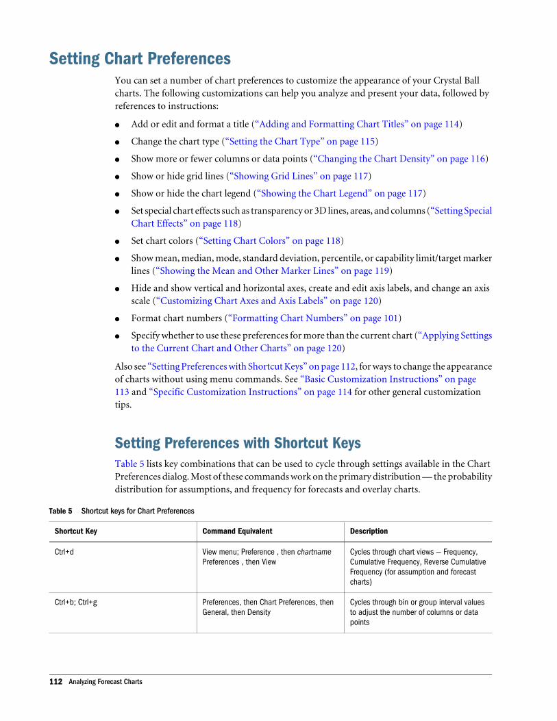
Setting Chart PreferencesYou can set a number of chart preferences to customize the appearance of your Crystal Ballcharts. The following customizations can help you analyze and present your data, followed byreferences to instructions:
l Add or edit and format a title (“Adding and Formatting Chart Titles” on page 114)
l Change the chart type (“Setting the Chart Type” on page 115)
l Show more or fewer columns or data points (“Changing the Chart Density” on page 116)
l Show or hide grid lines (“Showing Grid Lines” on page 117)
l Show or hide the chart legend (“Showing the Chart Legend” on page 117)
l Set special chart effects such as transparency or 3D lines, areas, and columns (“Setting SpecialChart Effects” on page 118)
l Set chart colors (“Setting Chart Colors” on page 118)
l Show mean, median, mode, standard deviation, percentile, or capability limit/target markerlines (“Showing the Mean and Other Marker Lines” on page 119)
l Hide and show vertical and horizontal axes, create and edit axis labels, and change an axisscale (“Customizing Chart Axes and Axis Labels” on page 120)
l Format chart numbers (“Formatting Chart Numbers” on page 101)
l Specify whether to use these preferences for more than the current chart (“Applying Settingsto the Current Chart and Other Charts” on page 120)
Also see “Setting Preferences with Shortcut Keys” on page 112, for ways to change the appearanceof charts without using menu commands. See “Basic Customization Instructions” on page113 and “Specific Customization Instructions” on page 114 for other general customizationtips.
Setting Preferences with Shortcut KeysTable 5 lists key combinations that can be used to cycle through settings available in the ChartPreferences dialog. Most of these commands work on the primary distribution — the probabilitydistribution for assumptions, and frequency for forecasts and overlay charts.
Table 5 Shortcut keys for Chart Preferences
Shortcut Key Command Equivalent Description
Ctrl+d View menu; Preference , then chartnamePreferences , then View
Cycles through chart views — Frequency,Cumulative Frequency, Reverse CumulativeFrequency (for assumption and forecastcharts)
Ctrl+b; Ctrl+g Preferences, then Chart Preferences, thenGeneral, then Density
Cycles through bin or group interval valuesto adjust the number of columns or datapoints
112 Analyzing Forecast Charts

Shortcut Key Command Equivalent Description
Ctrl+l Preferences, then Chart Preferences, thenGeneral, then Gridlines
Cycles through gridline settings: None,Horizontal, Vertical, Both
Ctrl+t Preferences, then Chart Preferences, thenChart Type, then Type
Cycles through chart types: Area, Line,Column; for sensitivity charts: Bar(direction), Bar (magnitude), Pie (inContribution To Variance view)
Ctrl+3 Preferences, then Chart Preferences, thenGeneral, then 3D Chart
Cycles between two-dimensional and three-dimensional chart display
Ctrl+m Preferences, then Chart Preferences, thenChart Type, then Marker Lines, then centraltendencies
Cycles through central tendency markerlines: None, Mean, Median, Mode (exceptfor sensitivity and trend charts)
Ctrl+n Preferences, then Chart Preferences, thenGeneral, then Legend
Toggles the legend display on and off
Ctrl+p Preferences, then Chart Preferences, thenChart Type, then Marker Lines, thenPercentiles
Cycles through percentile marker lines:None, 10%, 20%,…90%
Spacebar View menu; Preferences, then chartnamePreferences
Cycles through window views: Chart,Statistics, Percentiles, Goodness Of Fit (ifdistribution fitting is selected — except fortrend charts)
Basic Customization InstructionsThese instructions apply most specifically to forecast charts. However, many of them apply toother charts as well. For that reason, they are as general as possible, although not all settings willapply to every type of chart.
ä To customize a chart:
1 Create or display a chart and be sure it is the active chart window.
2 Either double-click the chart or choose Preferences, then Chart Preferences from the chart’s menubar.
The Chart Preferences dialog opens. Tab contents are as follows:
l General — Chart title, overall appearance of the chart
l Chart Type — Data sets (series) to display in the chart, chart type and color of plotted series,marker lines to display (optional)
l Axis — Vertical and horizontal axes to display, axis labels, axis scales, and axis numberformats
3 Make appropriate settings.
4 Optional step: To apply the settings to more than one chart, click Apply To. Then, specify whether to applyall chart preferences or just the current tab and whether to apply them to the current Excel sheet, all sheetsin the workbook, or all open and new workbooks and click OK. Otherwise, go to step 5.
Setting Chart Preferences 113
5 Click OK to apply the settings on all tabs to the active chart.
For a list of customizations you can perform on each tab, see “Specific CustomizationInstructions” on page 114.
Specific Customization InstructionsThis section explains how you can customize each part of your Crystal Ball charts to present theinformation most effectively. Topics for each Chart Preferences dialog tab are as follows.
General tab:
l “Adding and Formatting Chart Titles” on page 114
l “Changing the Chart Density” on page 116
l “Showing Grid Lines” on page 117
l “Showing the Chart Legend” on page 117
l “Setting Special Chart Effects” on page 118
Chart Type tab:
l “Setting the Chart Type” on page 115
l “Setting Chart Colors” on page 118
l “Showing the Mean and Other Marker Lines” on page 119
Axis tab:
l “Customizing Chart Axes and Axis Labels” on page 120
All tabs:
l “Applying Settings to the Current Chart and Other Charts” on page 120
For basic chart customization instructions, see “Basic Customization Instructions” on page113.
Adding and Formatting Chart Titles
ä To add or change a chart title:
1 Display the General tab of the Chart Preferences dialog.
The Chart Title group is displayed at the top of the General page.
By default, Auto is checked and a default title is displayed.
2 To edit the title, uncheck Auto and type the new title in the text box.
3 When all your settings are complete, click OK.
The chart is displayed with your new settings.
114 Analyzing Forecast Charts
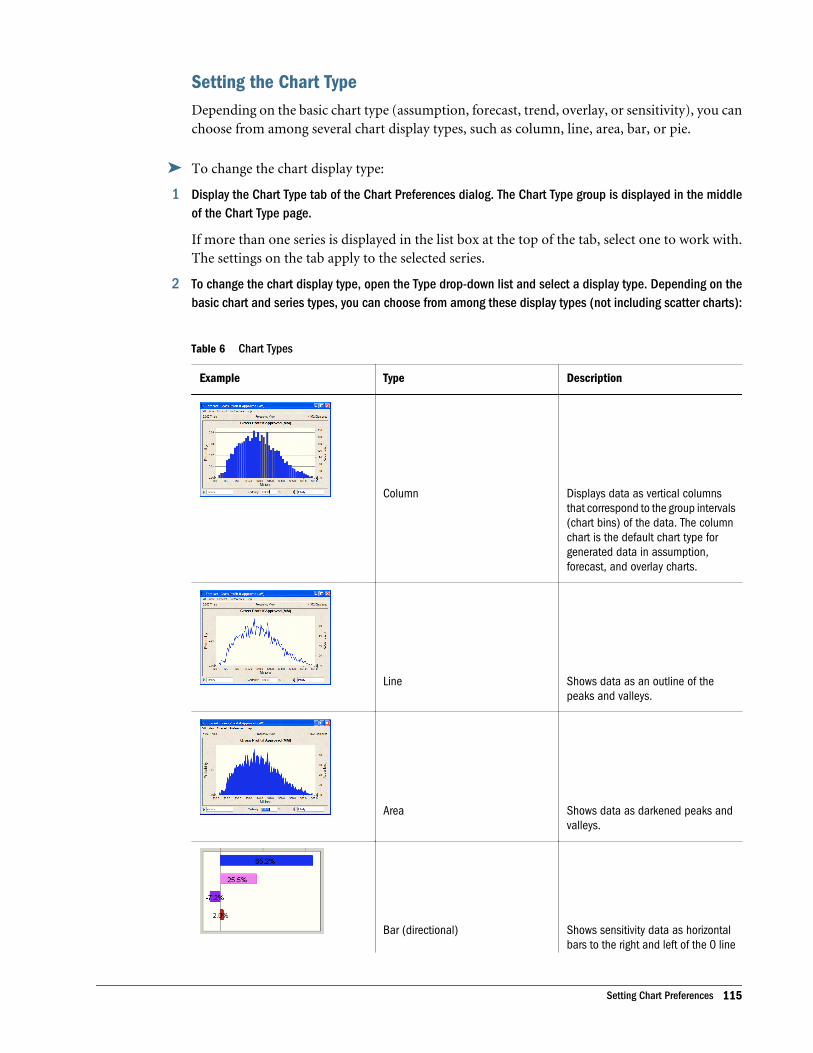
Setting the Chart TypeDepending on the basic chart type (assumption, forecast, trend, overlay, or sensitivity), you canchoose from among several chart display types, such as column, line, area, bar, or pie.
ä To change the chart display type:
1 Display the Chart Type tab of the Chart Preferences dialog. The Chart Type group is displayed in the middleof the Chart Type page.
If more than one series is displayed in the list box at the top of the tab, select one to work with.The settings on the tab apply to the selected series.
2 To change the chart display type, open the Type drop-down list and select a display type. Depending on thebasic chart and series types, you can choose from among these display types (not including scatter charts):
Table 6 Chart Types
Example Type Description
Column Displays data as vertical columnsthat correspond to the group intervals(chart bins) of the data. The columnchart is the default chart type forgenerated data in assumption,forecast, and overlay charts.
Line Shows data as an outline of thepeaks and valleys.
Area Shows data as darkened peaks andvalleys.
Bar (directional) Shows sensitivity data as horizontalbars to the right and left of the 0 line
Setting Chart Preferences 115
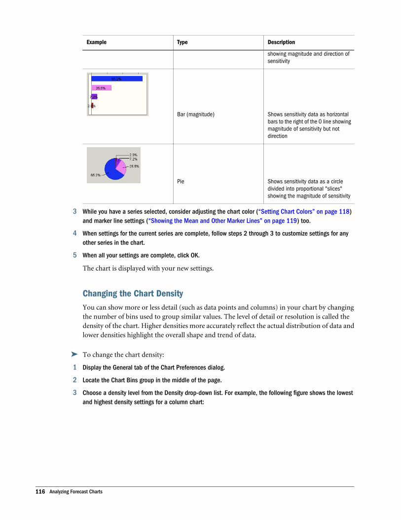
Example Type Description
showing magnitude and direction ofsensitivity
Bar (magnitude) Shows sensitivity data as horizontalbars to the right of the 0 line showingmagnitude of sensitivity but notdirection
Pie Shows sensitivity data as a circledivided into proportional "slices"showing the magnitude of sensitivity
3 While you have a series selected, consider adjusting the chart color (“Setting Chart Colors” on page 118)and marker line settings (“Showing the Mean and Other Marker Lines” on page 119) too.
4 When settings for the current series are complete, follow steps 2 through 3 to customize settings for anyother series in the chart.
5 When all your settings are complete, click OK.
The chart is displayed with your new settings.
Changing the Chart DensityYou can show more or less detail (such as data points and columns) in your chart by changingthe number of bins used to group similar values. The level of detail or resolution is called thedensity of the chart. Higher densities more accurately reflect the actual distribution of data andlower densities highlight the overall shape and trend of data.
ä To change the chart density:
1 Display the General tab of the Chart Preferences dialog.
2 Locate the Chart Bins group in the middle of the page.
3 Choose a density level from the Density drop-down list. For example, the following figure shows the lowestand highest density settings for a column chart:
116 Analyzing Forecast Charts
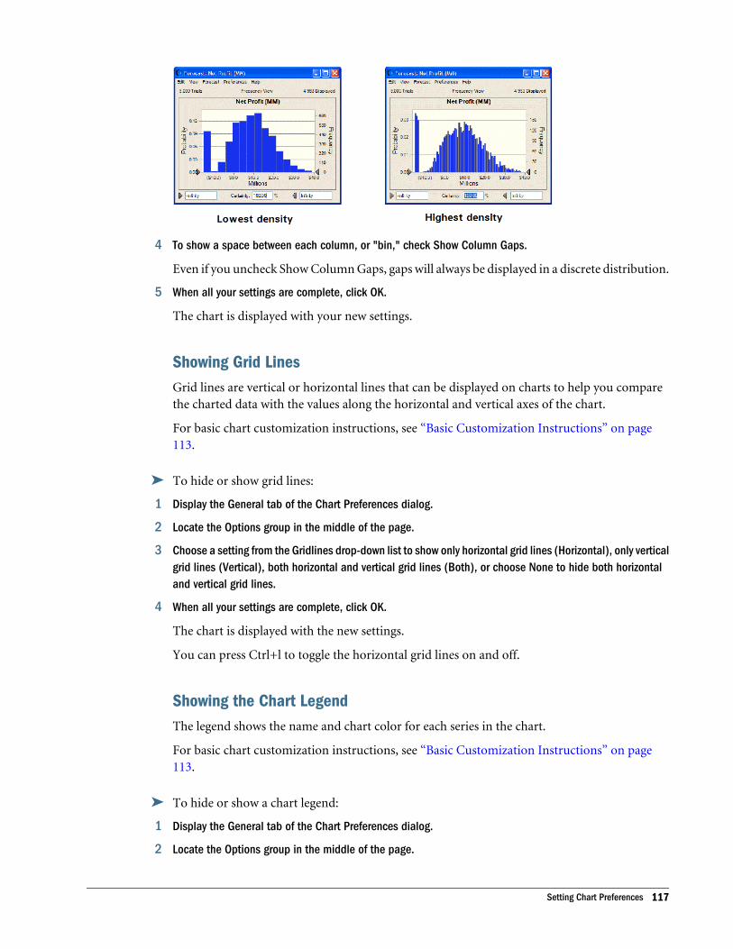
4 To show a space between each column, or "bin," check Show Column Gaps.
Even if you uncheck Show Column Gaps, gaps will always be displayed in a discrete distribution.
5 When all your settings are complete, click OK.
The chart is displayed with your new settings.
Showing Grid LinesGrid lines are vertical or horizontal lines that can be displayed on charts to help you comparethe charted data with the values along the horizontal and vertical axes of the chart.
For basic chart customization instructions, see “Basic Customization Instructions” on page113.
ä To hide or show grid lines:
1 Display the General tab of the Chart Preferences dialog.
2 Locate the Options group in the middle of the page.
3 Choose a setting from the Gridlines drop-down list to show only horizontal grid lines (Horizontal), only verticalgrid lines (Vertical), both horizontal and vertical grid lines (Both), or choose None to hide both horizontaland vertical grid lines.
4 When all your settings are complete, click OK.
The chart is displayed with the new settings.
You can press Ctrl+l to toggle the horizontal grid lines on and off.
Showing the Chart LegendThe legend shows the name and chart color for each series in the chart.
For basic chart customization instructions, see “Basic Customization Instructions” on page113.
ä To hide or show a chart legend:
1 Display the General tab of the Chart Preferences dialog.
2 Locate the Options group in the middle of the page.
Setting Chart Preferences 117
3 Choose a setting from the Legend drop-down list to show the legend at the right side of the chart (Right),the left side of the chart (Left), or the bottom of the chart (Bottom). To hide the legend, choose None.
4 When all your settings are complete, click OK.
The chart is displayed with the new settings.
You can press Ctrl+n to toggle the legend on and off.
Setting Special Chart EffectsYou can use special effects to help present your data most effectively. Transparency ensures thatall chart series and values are visible and 3D effects add graphic depth that can be so useful whenmany series are charted (for example, bars become blocks as shown in the chart density figurein “Changing the Chart Density” on page 116).
For basic chart customization instructions, see “Basic Customization Instructions” on page113.
ä To set special chart effects:
1 Display the General tab of the Chart Preferences dialog.
2 Locate the Effects group at the bottom of the page.
3 You can check any or all of the available effects to see how they enhance your chart. If you check Transparency,you can also choose a percent. 0% is completely opaque and 100% is completely transparent.
4 When all your settings are complete, click OK.
The chart is displayed with the new settings.
You can press Ctrl+3 to toggle 3D display on and off.
Setting Chart ColorsThis preference sets the color of the current chart series. This is the color that is displayed forthe series in the chart legend, if visible.
For basic chart customization instructions, see “Basic Customization Instructions” on page113.
ä To change the chart colors:
1 Display the Chart Type tab of the Chart Preferences dialog. The Chart group is displayed in the middle of theChart Type page.
If more than one series is displayed in the list box at the top of the tab, select one to work with.The settings on the page apply to the selected series.
2 Open the Color drop-down list and choose a color.
3 While you have a series selected, consider adjusting the chart type (“Setting the Chart Type” on page 115)and marker line settings (“Showing the Mean and Other Marker Lines” on page 119) too.
118 Analyzing Forecast Charts
4 When settings for the current series are complete, follow steps 2 through 3 to customize settings for anyother series in the chart.
5 When all your settings are complete, click OK.
The chart is displayed with your new settings.
Showing the Mean and Other Marker LinesYou can display mean, mode, median, standard deviation, and other marker lines onassumption, forecast, and overlay charts. These lines help you locate various values in the charteddistribution.
Note: If you have activated the process capability features and have entered an LSL, USL, orTarget value, you can include marker lines for them in your forecast chart (“Viewing LSL,USL, and Target Marker Lines” on page 391).
Base Case is the value in an assumption, decision variable, or forecast cell prior to running thesimulation. For forecasts, Certainty Range shows lines at the certainty range endpoints. Markerlines are shown with labels, such as Mean = $125.
You can press Ctrl+m to cycle through the median, mean, and base case or mode, dependingon chart type. Press Ctrl+p to cycle through every 10th percentile.
ä To display marker lines:
1 Display the Chart Type tab of the Chart Preferences dialog. The Marker Lines group is displayed in the lowerright corner of Chart Type.
If more than one series is displayed in the list box at the top of the tab, select one to work with.The settings on the page apply to the selected series.
2 To display a marker line, check the box for that item. If you choose Standard Deviation, Percentile, orValue, another dialog opens:
l For Standard Deviation, enter the standard deviation(s) where you want a marker to bedisplayed. If you enter more than one, separate them with commas. Then, choose whetheryou want the marker(s) to bedisplayed below the mean (technically indicating negativestandard deviations), above the mean, or both above and below.
l For Percentile, select the group of percentiles where you want markers to be displayed orchoose Custom and create your own group of percentile points separated by commas.
l For Value, enter the x-axis value where the line should be displayed in the Value field andclick Add. If you want, enter an optional label and check Show Value On Marker Line todisplay the value on the chart. You can click New to add another value.
3 While you have a series selected, consider adjusting the chart type (“Setting the Chart Type” on page 115)and color (“Setting Chart Colors” on page 118) too.
4 When settings for the current series are complete, follow steps 2 and 3 to customize settings for any otherseries in the chart.
Setting Chart Preferences 119
5 When all your settings are complete, click OK.
The chart is displayed with your new settings.
If the marker lines fall outside the maximum or minimum value displayed on a chart, they willnot be displayed on the chart. For example, this can happen with standard deviations of plus orminus 2 or 3 for uniform distributions.
Customizing Chart Axes and Axis LabelsYou can customize the label, scale, and format of the main axis in Crystal Ball charts.
ä To customize chart axes:
1 Display the Axis tab of the Chart Preferences dialog.
2 Consider the label to use for the axis.
By default, Auto is checked in the Axis Label group. A label is automatically assigned dependingon the chart type. For example, the value (x) axis of a forecast chart uses the Units entry in theDefine Forecast dialog as the label. To enter a custom axis label, uncheck Auto and type a moredescriptive label in the edit field.
3 Next, adjust the Scale settings. By default, Auto is displayed in the Type list and the chart is displayed withthe most appropriate end points for that chart type. To use another scale, choose it from the Type drop-downlist and enter the minimum (Min) and maximum (Max) values to use for the scale.
Most chart/axis combinations offer Fixed as an alternative. The value axis for assumption,forecast, and overlay charts also offers Standard Deviation and Percentile.
4 The Format Number settings control the format of the axis label numbers. Choose appropriate settings foryour chart.
l For Format settings, Cell Format uses the format of the underlying cell. Most choices aresimilar to those used in Excel: General, Number, Currency, Scientific, Percentage, or Date.
l The Decimal settings control the number of decimal points.
l When checked, Thousand Separator inserts a thousands-separator symbol whereappropriate (except when Scientific formatting is set). The thousands separator that isdisplayed is the one defined in Windows International or Regional Options settings.
The Format Number settings also control the format of assumption parameters in the DefineAssumption dialog and assumption charts.
5 When all your settings are complete, click OK.
The chart is displayed with your new settings.
Applying Settings to the Current Chart and Other ChartsIf you would like to apply the current settings to other charts in your model, you can choosewhat to apply and where to apply them. (These instructions apply anywhere the Apply To buttonis displayed.)
120 Analyzing Forecast Charts
ä To specify how chart settings should be applied:
1 Click the Apply To button.
The Apply To dialog opens.
2 Indicate the tab or tabs of settings to apply:
l This Tab applies only settings on the current tab.
l All Tabs applies all the current settings on the entire dialog.
3 Indicate where the settings should be applied.
l This Sheet applies the settings to only the current sheet of the current workbook.
l This Workbook applies the settings to all sheets of the current workbook.
l All Open And New Workbooks applies the settings to all workbooks that are currently openand all workbooks to be created.
All Workbooks effectively changes the global Chart Preferences defaults to the settings onthe current tab or all tabs, depending on the setting in the previous dialog group.
Apply To settings are both flexible and powerful. They can be used as focused or broaddefaults.
Managing Existing ChartsPrevious sections of this chapter have described how to create and customize new charts. Thefollowing sections describe how to open, copy, paste, print, close, and delete existing charts:
l “Opening Charts” on page 121
l “Copying and Pasting Charts to Other Applications” on page 122
l “Printing Charts” on page 123
l “Closing Charts” on page 123
l “Deleting Charts” on page 124
Opening ChartsAfter you create an assumption or forecast chart, it is saved with the workbook that contains it.Other charts are saved with the active workbook model. You can display charts again, withcurrent data, anytime you rerun the model with associated workbooks open.
ä To open a chart:
1 Open the model containing the chart and run a simulation or restore saved results (“Restoring Crystal BallSimulation Results” on page 87).
2 Open the Analyze menu and select the type of chart to display: Assumption Charts, Forecast Charts, OverlayCharts, Trend Charts, or Sensitivity Charts.
3 When the dialog for that chart opens, check the box in front of each chart to display.
Managing Existing Charts 121
4 Click Open.
You might need to click the Crystal Ball and Microsoft Excel icons in the Windowstask bar to activate charts that have disappeared behind the spreadsheet.
In Excel 2007, choose Analyze, then View Charts, then Forecast Charts.
To open a number of charts at one time, select the Crystal Ball data cells and choose Analyze,then Open Selected Cells. All charts for the selected cells open and are displayed in front of anyother open charts. In Excel 2007, choose Analyze, then View Charts, then Open From Selection.
Copying and Pasting Charts to Other ApplicationsYou can copy and paste assumption, forecast, overlay, trend, and sensitivity charts to otherapplications such as Microsoft Word, Powerpoint, and Excel.
For instructions, see the following sections:
l “Copying Charts” on page 122
l “Pasting Charts from the Clipboard” on page 122
Copying Charts
ä To copy charts for use in other applications:
1 Select the chart to copy.
2 Open its View menu and choose the view to be copied.
If you choose a data view such as Percentiles, Statistics, or Goodness Of Fit, the data will bepasted into many applications as alphanumeric data, ready to edit, add, and so on. This is truefor Microsoft Excel and Word, but not Powerpoint. Data is pasted into Powerpoint as a graphic.
Graphic views, such as Frequency, are pasted as bitmap images.
3 In the chart’s menubar, choose Edit, then Copy.
The chart is copied to the Clipboard, ready to paste into another application.
Pasting Charts from the Clipboard
ä To paste a chart into another application using its own Paste commands:
1 Copy the Crystal Ball chart as described in the previous section.
2 Open a document (spreadsheet, slide, and so on) in the application to receive the chart.
3 Within that application, choose Edit, then Paste or Edit, then Paste Special.
(To paste in Excel 2007, press Ctrl+v or click the Home tab and choose Clipboard, then Pasteat the left end of the ribbon.)
122 Analyzing Forecast Charts

As described above, if you copied a data view such as Percentiles, Statistics, or Goodness of Fit,the data is pasted into many applications as editable numbers or text.
Graphic views, such as Frequency, are pasted as bitmap images.
Printing Charts
ä To print a chart, display it and choose Edit, then Print in the chart’s menubar.
Before printing, can choose Edit, then Page Setup to format the chart on the page. Then, chooseEdit, then Print Preview to view the chart as it will print on the selected paper size.
For example, Figure 35 shows the Print Preview dialog for a forecast chart from Toxic WasteSite.xls in Landscape orientation on Letter paper.
Figure 35 Print Preview Dialog for a Forecast Chart
Closing ChartsWhen you close a chart, you remove it from memory but do not delete it permanently.
ä To close a chart:
1 Open the Analyze menu and select the type of chart to close.
If you are using Crystal Ball in Excel 2007, choose Analyze, then View Charts and then choosea command.
2 When the dialog for that chart opens, check the box in front of each chart to close.
3 Click Close.
The selected chart or charts are closed without prompting.
Managing Existing Charts 123

You can use Analyze, then Close All to close all chart windows from the current simulation andrestored results. In Excel 2007, choose Analyze, then View Charts, then Close All.
Deleting ChartsYou do not need to open a chart to delete it, as long as the model or saved results file containingit is open.
ä To delete a chart (except assumption and forecast charts):
1 Open the model containing the chart.
2 Open the Analyze menu and select the type of chart to delete.
If you are using Crystal Ball in Excel 2007, choose Analyze, then View Charts and then choosea chart type.
3 When the dialog for that chart opens, check the box in front of each chart to delete.
4 Click Delete.
The selected chart or charts are deleted without prompting. Assumption and forecast chartscannot be deleted in this way.
124 Analyzing Forecast Charts
7Analyzing Other Charts
In This Chapter
Overview ... . . . . . . . . . . . . . . . . . . . . . . . . . . . . . . . . . . . . . . . . . . . . . . . . . . . . . . . . . . . . . . . . . . . . . . . . . . . . . . . . . . . . . . . . . . . . . . . . . . . . . . . . . . . . . . . . . . . . . . . 125
Understanding and Using Overlay Charts .. . . . . . . . . . . . . . . . . . . . . . . . . . . . . . . . . . . . . . . . . . . . . . . . . . . . . . . . . . . . . . . . . . . . . . . . . . . . . . . . . . . . . 126
Understanding and Using Trend Charts .. . . . . . . . . . . . . . . . . . . . . . . . . . . . . . . . . . . . . . . . . . . . . . . . . . . . . . . . . . . . . . . . . . . . . . . . . . . . . . . . . . . . . . . 131
Understanding and Using Sensitivity Charts.. . . . . . . . . . . . . . . . . . . . . . . . . . . . . . . . . . . . . . . . . . . . . . . . . . . . . . . . . . . . . . . . . . . . . . . . . . . . . . . . . . 138
Understanding and Using Assumption Charts.. . . . . . . . . . . . . . . . . . . . . . . . . . . . . . . . . . . . . . . . . . . . . . . . . . . . . . . . . . . . . . . . . . . . . . . . . . . . . . . . 147
Understanding and Using Scatter Charts .. . . . . . . . . . . . . . . . . . . . . . . . . . . . . . . . . . . . . . . . . . . . . . . . . . . . . . . . . . . . . . . . . . . . . . . . . . . . . . . . . . . . . 149
OverviewThe previous chapter gave guidelines for analyzing and customizing simulation results with afocus on forecast charts.
This chapter extends the information on analyzing simulation results provided in Chapter 6.You will learn how to use the following additional charts to interpret and present data:
l Overlay charts to view forecasts superimposed over each other (“Understanding and UsingOverlay Charts” on page 126)
l Trend charts to view the certainty ranges of all your forecasts on a single chart(“Understanding and Using Trend Charts” on page 131)
l Sensitivity charts to view the impact your assumptions have on forecast results(“Understanding and Using Sensitivity Charts” on page 138)
l Assumption charts to confirm random number sampling (“Understanding and UsingAssumption Charts” on page 147)
l Scatter charts to compare paired data (“Understanding and Using Scatter Charts” on page149)
If you have OptQuest, you can also display OptQuest charts with optimization results.
For information on customizing charts, managing chart windows, and printing charts, seeChapter 6.
Overview 125
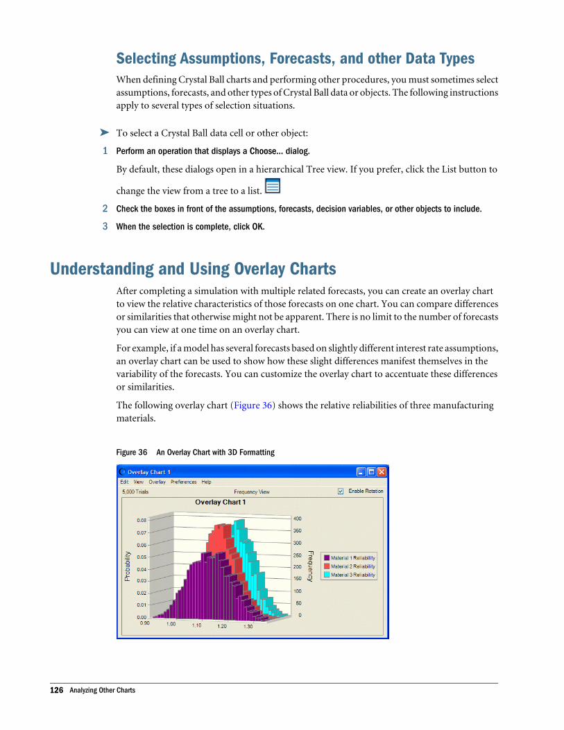
Selecting Assumptions, Forecasts, and other Data TypesWhen defining Crystal Ball charts and performing other procedures, you must sometimes selectassumptions, forecasts, and other types of Crystal Ball data or objects. The following instructionsapply to several types of selection situations.
ä To select a Crystal Ball data cell or other object:
1 Perform an operation that displays a Choose... dialog.
By default, these dialogs open in a hierarchical Tree view. If you prefer, click the List button to
change the view from a tree to a list.
2 Check the boxes in front of the assumptions, forecasts, decision variables, or other objects to include.
3 When the selection is complete, click OK.
Understanding and Using Overlay ChartsAfter completing a simulation with multiple related forecasts, you can create an overlay chartto view the relative characteristics of those forecasts on one chart. You can compare differencesor similarities that otherwise might not be apparent. There is no limit to the number of forecastsyou can view at one time on an overlay chart.
For example, if a model has several forecasts based on slightly different interest rate assumptions,an overlay chart can be used to show how these slight differences manifest themselves in thevariability of the forecasts. You can customize the overlay chart to accentuate these differencesor similarities.
The following overlay chart (Figure 36) shows the relative reliabilities of three manufacturingmaterials.
Figure 36 An Overlay Chart with 3D Formatting
126 Analyzing Other Charts
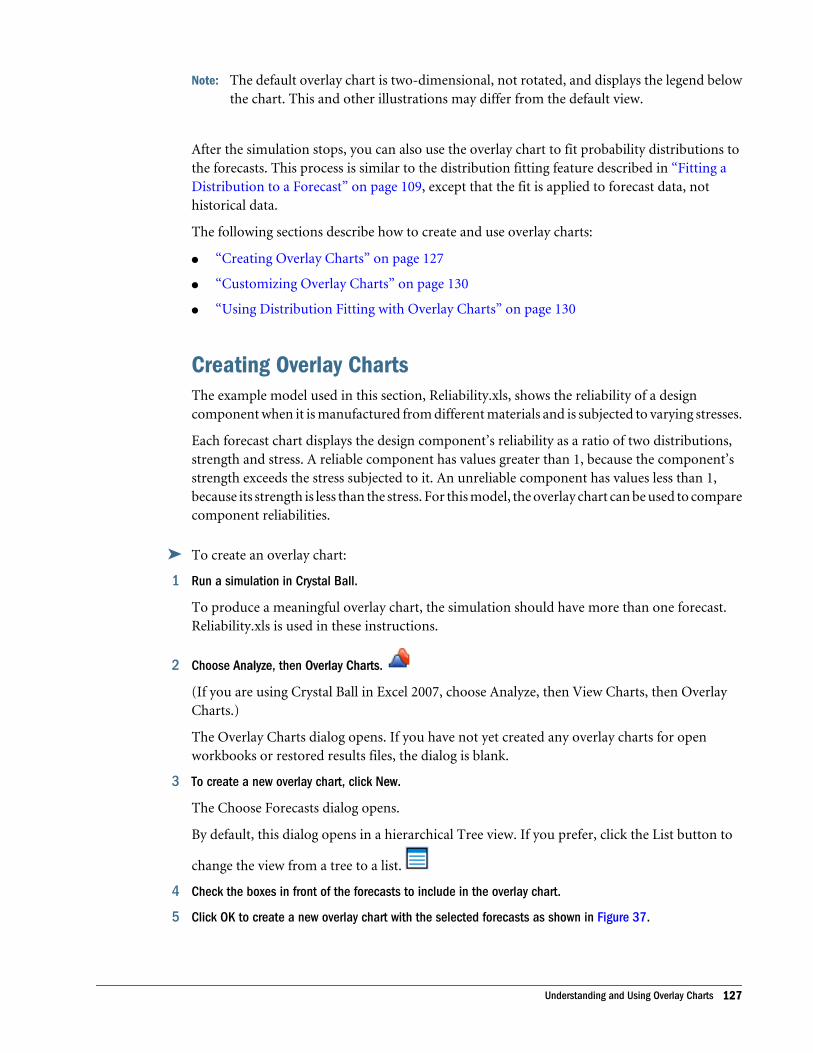
Note: The default overlay chart is two-dimensional, not rotated, and displays the legend belowthe chart. This and other illustrations may differ from the default view.
After the simulation stops, you can also use the overlay chart to fit probability distributions tothe forecasts. This process is similar to the distribution fitting feature described in “Fitting aDistribution to a Forecast” on page 109, except that the fit is applied to forecast data, nothistorical data.
The following sections describe how to create and use overlay charts:
l “Creating Overlay Charts” on page 127
l “Customizing Overlay Charts” on page 130
l “Using Distribution Fitting with Overlay Charts” on page 130
Creating Overlay ChartsThe example model used in this section, Reliability.xls, shows the reliability of a designcomponent when it is manufactured from different materials and is subjected to varying stresses.
Each forecast chart displays the design component’s reliability as a ratio of two distributions,strength and stress. A reliable component has values greater than 1, because the component’sstrength exceeds the stress subjected to it. An unreliable component has values less than 1,because its strength is less than the stress. For this model, the overlay chart can be used to comparecomponent reliabilities.
ä To create an overlay chart:
1 Run a simulation in Crystal Ball.
To produce a meaningful overlay chart, the simulation should have more than one forecast.Reliability.xls is used in these instructions.
2 Choose Analyze, then Overlay Charts.
(If you are using Crystal Ball in Excel 2007, choose Analyze, then View Charts, then OverlayCharts.)
The Overlay Charts dialog opens. If you have not yet created any overlay charts for openworkbooks or restored results files, the dialog is blank.
3 To create a new overlay chart, click New.
The Choose Forecasts dialog opens.
By default, this dialog opens in a hierarchical Tree view. If you prefer, click the List button to
change the view from a tree to a list.
4 Check the boxes in front of the forecasts to include in the overlay chart.
5 Click OK to create a new overlay chart with the selected forecasts as shown in Figure 37.
Understanding and Using Overlay Charts 127
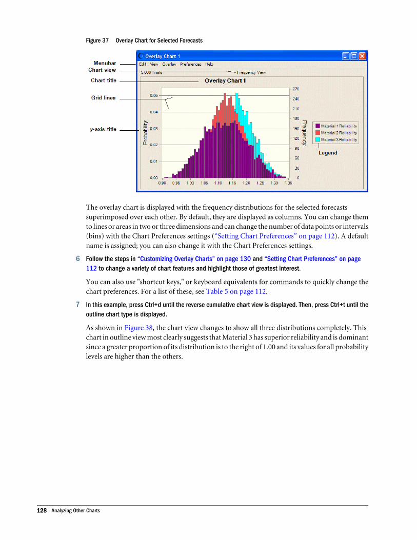
Figure 37 Overlay Chart for Selected Forecasts
The overlay chart is displayed with the frequency distributions for the selected forecastssuperimposed over each other. By default, they are displayed as columns. You can change themto lines or areas in two or three dimensions and can change the number of data points or intervals(bins) with the Chart Preferences settings (“Setting Chart Preferences” on page 112). A defaultname is assigned; you can also change it with the Chart Preferences settings.
6 Follow the steps in “Customizing Overlay Charts” on page 130 and “Setting Chart Preferences” on page112 to change a variety of chart features and highlight those of greatest interest.
You can also use "shortcut keys," or keyboard equivalents for commands to quickly change thechart preferences. For a list of these, see Table 5 on page 112.
7 In this example, press Ctrl+d until the reverse cumulative chart view is displayed. Then, press Ctrl+t until theoutline chart type is displayed.
As shown in Figure 38, the chart view changes to show all three distributions completely. Thischart in outline view most clearly suggests that Material 3 has superior reliability and is dominantsince a greater proportion of its distribution is to the right of 1.00 and its values for all probabilitylevels are higher than the others.
128 Analyzing Other Charts
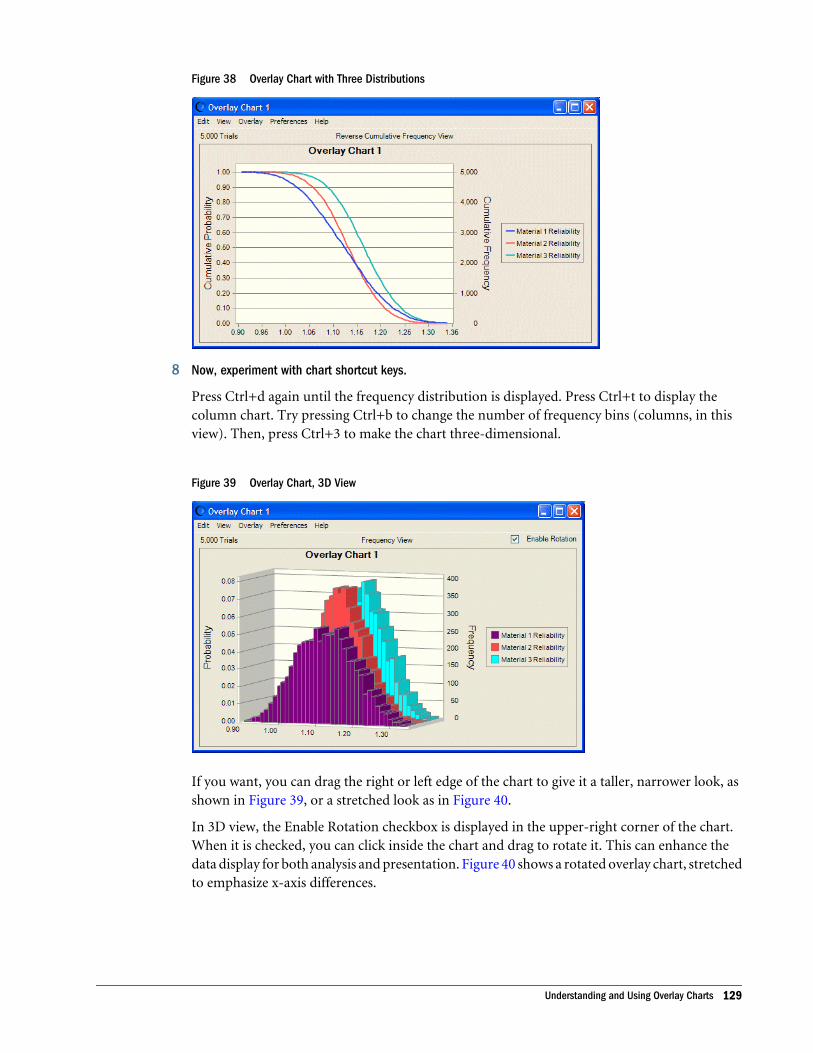
Figure 38 Overlay Chart with Three Distributions
8 Now, experiment with chart shortcut keys.
Press Ctrl+d again until the frequency distribution is displayed. Press Ctrl+t to display thecolumn chart. Try pressing Ctrl+b to change the number of frequency bins (columns, in thisview). Then, press Ctrl+3 to make the chart three-dimensional.
Figure 39 Overlay Chart, 3D View
If you want, you can drag the right or left edge of the chart to give it a taller, narrower look, asshown in Figure 39, or a stretched look as in Figure 40.
In 3D view, the Enable Rotation checkbox is displayed in the upper-right corner of the chart.When it is checked, you can click inside the chart and drag to rotate it. This can enhance thedata display for both analysis and presentation. Figure 40 shows a rotated overlay chart, stretchedto emphasize x-axis differences.
Understanding and Using Overlay Charts 129
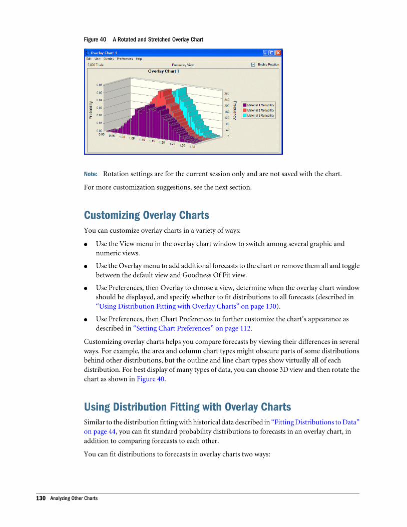
Figure 40 A Rotated and Stretched Overlay Chart
Note: Rotation settings are for the current session only and are not saved with the chart.
For more customization suggestions, see the next section.
Customizing Overlay ChartsYou can customize overlay charts in a variety of ways:
l Use the View menu in the overlay chart window to switch among several graphic andnumeric views.
l Use the Overlay menu to add additional forecasts to the chart or remove them all and togglebetween the default view and Goodness Of Fit view.
l Use Preferences, then Overlay to choose a view, determine when the overlay chart windowshould be displayed, and specify whether to fit distributions to all forecasts (described in“Using Distribution Fitting with Overlay Charts” on page 130).
l Use Preferences, then Chart Preferences to further customize the chart’s appearance asdescribed in “Setting Chart Preferences” on page 112.
Customizing overlay charts helps you compare forecasts by viewing their differences in severalways. For example, the area and column chart types might obscure parts of some distributionsbehind other distributions, but the outline and line chart types show virtually all of eachdistribution. For best display of many types of data, you can choose 3D view and then rotate thechart as shown in Figure 40.
Using Distribution Fitting with Overlay ChartsSimilar to the distribution fitting with historical data described in “Fitting Distributions to Data”on page 44, you can fit standard probability distributions to forecasts in an overlay chart, inaddition to comparing forecasts to each other.
You can fit distributions to forecasts in overlay charts two ways:
130 Analyzing Other Charts
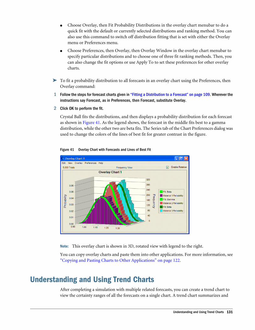
l Choose Overlay, then Fit Probability Distributions in the overlay chart menubar to do aquick fit with the default or currently selected distributions and ranking method. You canalso use this command to switch off distribution fitting that is set with either the Overlaymenu or Preferences menu.
l Choose Preferences, then Overlay, then Overlay Window in the overlay chart menubar tospecify particular distributions and to choose one of three fit ranking methods. Then, youcan also change the fit options or use Apply To to set these preferences for other overlaycharts.
ä To fit a probability distribution to all forecasts in an overlay chart using the Preferences, thenOverlay command:
1 Follow the steps for forecast charts given in “Fitting a Distribution to a Forecast” on page 109. Wherever theinstructions say Forecast, as in Preferences, then Forecast, substitute Overlay.
2 Click OK to perform the fit.
Crystal Ball fits the distributions, and then displays a probability distribution for each forecastas shown in Figure 41. As the legend shows, the forecast in the middle fits best to a gammadistribution, while the other two are beta fits. The Series tab of the Chart Preferences dialog wasused to change the colors of the lines of best fit for greater contrast in the figure.
Figure 41 Overlay Chart with Forecasts and Lines of Best Fit
Note: This overlay chart is shown in 3D, rotated view with legend to the right.
You can copy overlay charts and paste them into other applications. For more information, see“Copying and Pasting Charts to Other Applications” on page 122.
Understanding and Using Trend ChartsAfter completing a simulation with multiple related forecasts, you can create a trend chart toview the certainty ranges of all the forecasts on a single chart. A trend chart summarizes and
Understanding and Using Trend Charts 131
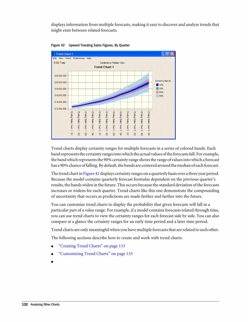
displays information from multiple forecasts, making it easy to discover and analyze trends thatmight exist between related forecasts.
Figure 42 Upward Trending Sales Figures, By Quarter
Trend charts display certainty ranges for multiple forecasts in a series of colored bands. Eachband represents the certainty ranges into which the actual values of the forecasts fall. For example,the band which represents the 90% certainty range shows the range of values into which a forecasthas a 90% chance of falling. By default, the bands are centered around the median of each forecast.
The trend chart in Figure 42 displays certainty ranges on a quarterly basis over a three year period.Because the model contains quarterly forecast formulas dependent on the previous quarter’sresults, the bands widen in the future. This occurs because the standard deviation of the forecastsincreases or widens for each quarter. Trend charts like this one demonstrate the compoundingof uncertainty that occurs as predictions are made farther and farther into the future.
You can customize trend charts to display the probability that given forecasts will fall in aparticular part of a value range. For example, if a model contains forecasts related through time,you can use trend charts to view the certainty ranges for each forecast side by side. You can alsocompare at a glance the certainty ranges for an early time period and a later time period.
Trend charts are only meaningful when you have multiple forecasts that are related to each other.
The following sections describe how to create and work with trend charts:
l “Creating Trend Charts” on page 133
l “Customizing Trend Charts” on page 133
l
132 Analyzing Other Charts
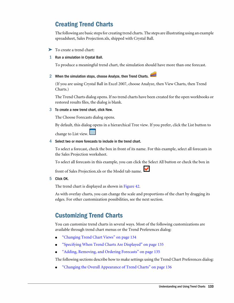
Creating Trend ChartsThe following are basic steps for creating trend charts. The steps are illustrating using an examplespreadsheet, Sales Projection.xls, shipped with Crystal Ball.
ä To create a trend chart:
1 Run a simulation in Crystal Ball.
To produce a meaningful trend chart, the simulation should have more than one forecast.
2 When the simulation stops, choose Analyze, then Trend Charts.
(If you are using Crystal Ball in Excel 2007, choose Analyze, then View Charts, then TrendCharts.)
The Trend Charts dialog opens. If no trend charts have been created for the open workbooks orrestored results files, the dialog is blank.
3 To create a new trend chart, click New.
The Choose Forecasts dialog opens.
By default, this dialog opens in a hierarchical Tree view. If you prefer, click the List button to
change to List view.
4 Select two or more forecasts to include in the trend chart.
To select a forecast, check the box in front of its name. For this example, select all forecasts inthe Sales Projection worksheet.
To select all forecasts in this example, you can click the Select All button or check the box in
front of Sales Projection.xls or the Model tab name.
5 Click OK.
The trend chart is displayed as shown in Figure 42.
As with overlay charts, you can change the scale and proportions of the chart by dragging itsedges. For other customization possibilities, see the next section.
Customizing Trend ChartsYou can customize trend charts in several ways. Most of the following customizations areavailable through trend chart menus or the Trend Preferences dialog:
l “Changing Trend Chart Views” on page 134
l “Specifying When Trend Charts Are Displayed” on page 135
l “Adding, Removing, and Ordering Forecasts” on page 135
The following sections describe how to make settings using the Trend Chart Preferences dialog:
l “Changing the Overall Appearance of Trend Charts” on page 136
Understanding and Using Trend Charts 133
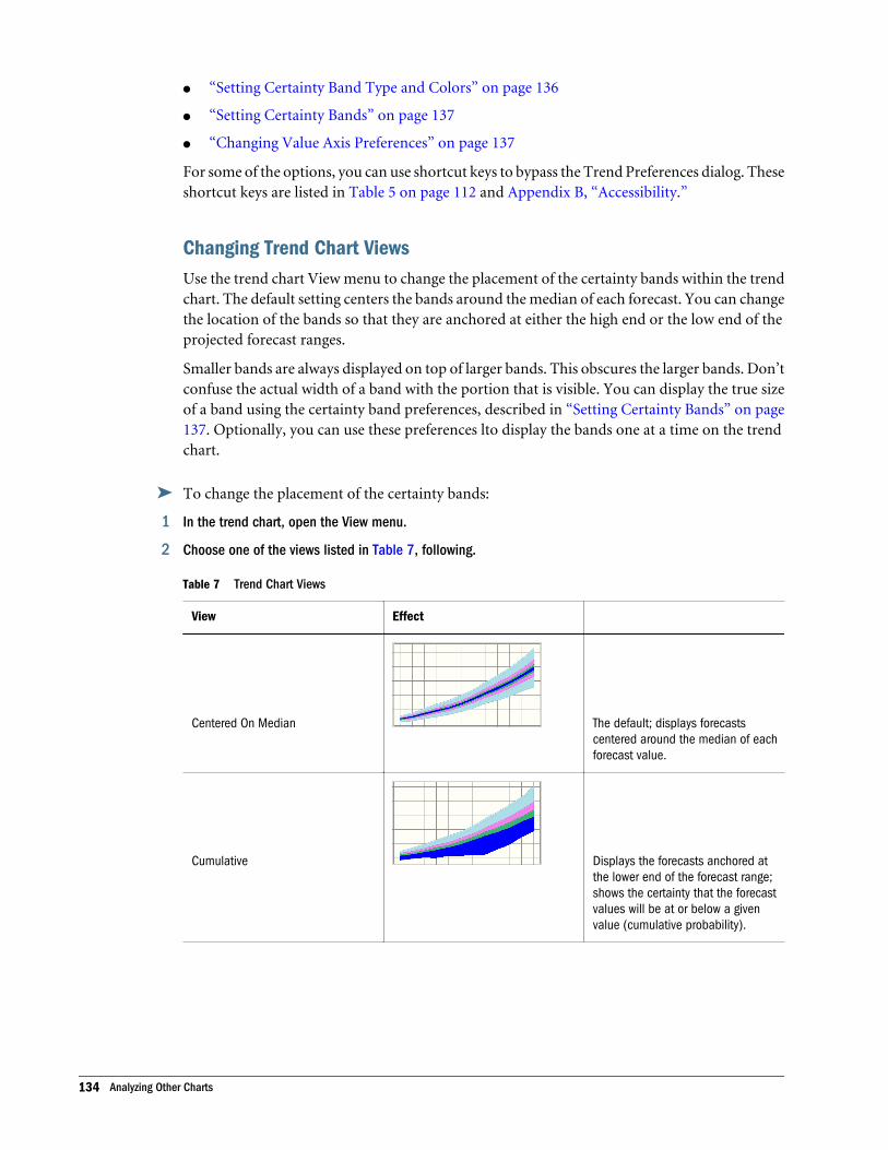
l “Setting Certainty Band Type and Colors” on page 136
l “Setting Certainty Bands” on page 137
l “Changing Value Axis Preferences” on page 137
For some of the options, you can use shortcut keys to bypass the Trend Preferences dialog. Theseshortcut keys are listed in Table 5 on page 112 and Appendix B, “Accessibility.”
Changing Trend Chart ViewsUse the trend chart View menu to change the placement of the certainty bands within the trendchart. The default setting centers the bands around the median of each forecast. You can changethe location of the bands so that they are anchored at either the high end or the low end of theprojected forecast ranges.
Smaller bands are always displayed on top of larger bands. This obscures the larger bands. Don’tconfuse the actual width of a band with the portion that is visible. You can display the true sizeof a band using the certainty band preferences, described in “Setting Certainty Bands” on page137. Optionally, you can use these preferences lto display the bands one at a time on the trendchart.
ä To change the placement of the certainty bands:
1 In the trend chart, open the View menu.
2 Choose one of the views listed in Table 7, following.
Table 7 Trend Chart Views
View Effect
Centered On Median The default; displays forecastscentered around the median of eachforecast value.
Cumulative Displays the forecasts anchored atthe lower end of the forecast range;shows the certainty that the forecastvalues will be at or below a givenvalue (cumulative probability).
134 Analyzing Other Charts
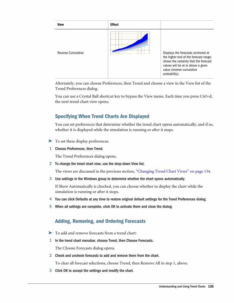
View Effect
Reverse Cumulative Displays the forecasts anchored atthe higher end of the forecast range;shows the certainty that the forecastvalues will be at or above a givenvalue (reverse cumulativeprobability).
Alternately, you can choose Preferences, then Trend and choose a view in the View list of theTrend Preferences dialog.
You can use a Crystal Ball shortcut key to bypass the View menu. Each time you press Ctrl+d,the next trend chart view opens.
Specifying When Trend Charts Are DisplayedYou can set preferences that determine whether the trend chart opens automatically, and if so,whether it is displayed while the simulation is running or after it stops.
ä To set these display preferences:
1 Choose Preferences, then Trend.
The Trend Preferences dialog opens.
2 To change the trend chart view, use the drop-down View list.
The views are discussed in the previous section, “Changing Trend Chart Views” on page 134.
3 Use settings in the Windows group to determine whether the chart opens automatically.
If Show Automatically is checked, you can choose whether to display the chart while thesimulation is running or after it stops.
4 You can click Defaults at any time to restore original default settings for the Trend Preferences dialog.
5 When all settings are complete, click OK to activate them and close the dialog.
Adding, Removing, and Ordering Forecasts
ä To add and remove forecasts from a trend chart:
1 In the trend chart menubar, choose Trend, then Choose Forecasts.
The Choose Forecasts dialog opens.
2 Check and uncheck forecasts to add and remove them from the chart.
To clear all forecast selections, choose Trend, then Remove All in step 1, above.
3 Click OK to accept the settings and modify the chart.
Understanding and Using Trend Charts 135
After you select forecasts and create a trend chart, you can change the order of forecast display.
ä To change the order of forecasts:
1 In the trend chart menubar, choose Preferences, then Chart, then Chart Type.
The Chart Type dialog opens.
All charted forecasts are displayed in the Series list at the top of the dialog. The forecast at thetop of the list is displayed as the first forecast at the left of the forecast axis.
2 Select a forecast in the list and use the up and down arrow keys to the right of the list to move the forecastup or down the list.
3 Optional step: You can choose Defaults at any time to restore all settings to their original default values.
4 Optional step: To apply the settings to more than one chart, click Apply To. Then, specify how they shouldbe applied (see “Applying Settings to the Current Chart and Other Charts” on page 120 for details) and clickOK. Otherwise, go to step 5.
5 When all forecasts are positioned in order, click OK to accept the current Chart Preferences settings andmodify the chart.
Changing the Overall Appearance of Trend ChartsWhen you first choose Preferences, then Chart in the trend chart menubar, the General tab ofthe Chart Preferences dialog opens.
Except for the disabled Chart Bins preferences, the General tab settings are the same as those forforecast and other charts.
You can set the following features, described in the sections in parentheses:
l Chart title (“Adding and Formatting Chart Titles” on page 114)
l Gridlines (“Showing Grid Lines” on page 117)
l Legend (“Showing the Chart Legend” on page 117)
l Chart effects (“Setting Special Chart Effects” on page 118)
For descriptions of each setting while you are viewing the dialog, click Help.
Setting Certainty Band Type and ColorsBy default, the trend chart certainty bands are displayed as solid-colored areas. You can changethe bands from solid areas to uncolored areas bordered by lines. You can also change the colorof each certainty band.
ä To change the chart type or color settings:
1 Choose Preferences, then Chart, then Chart Type.
The Chart Type tab of the Chart Preferences dialog opens.
2 To change all certainty bands from areas to lines, choose Line in the Chart Type drop-down list.
136 Analyzing Other Charts
3 To change the color of a certainty band:
a. Select the certainty band to change from the list below the Certainty Bands button.
b. Select a color from the Band Color list.
4 To select a different set of certainty levels or define your own, click the Certainty Bands button and followthe steps in the next section, “Setting Certainty Bands” on page 137
5 Optional: You can choose Defaults at any time to restore all settings to their original default values.
6 Optional: To apply the settings to more than one chart, click Apply To. Then, specify how they should beapplied (see “Applying Settings to the Current Chart and Other Charts” on page 120 for details) and clickOK. Otherwise, go to step 7.
7 When settings are complete, click OK to accept current settings on all tabs of the Chart Preferences dialog.
You can use the Chart Series list at the top of the Chart Type tab to change the order of forecastsin the forecast axis. For instructions, see “Adding, Removing, and Ordering Forecasts” on page135.
Setting Certainty BandsYou can easily choose a set of certainty bands (levels) to display in the trend chart or create yourown custom set.
ä To change or define a set of certainty bands:
1 In the trend chart menubar, choose Preferences, then Chart.
2 Click the Chart Type tab.
3 On the Chart Type tab, click the Certainty Bands button.
4 The Percentiles dialog opens.
5 Choose a set of certainty bands to display on the trend chart.
6 To create your own set, choose Custom and enter a series of certainty bands, separated by commas.
7 Click OK.
The trend chart opens with the selected certainty bands. A legend is displayed on the right sideof the trend chart indicating which levels are represented by which bands.
If the legend does not include all bands, drag the top or the bottom of the trend chart to increaseits height until all bands are displayed.
Changing Value Axis PreferencesYou can change several trend chart axis preferences, as described below. You can add a namefor the value axis, set number formats, and set value rounding. You can also change Scale settingsfrom Auto to Fixed and specify a range minimum and maximum value. You can use these scalesettings to display the probability that given forecasts will fall in a particular part of a value range.
Understanding and Using Trend Charts 137

ä To change value axis settings:
1 In the trend chart menubar, choose Preferences, then Chart, then Axis.
The Axis tab of the Chart Preferences dialog opens.
2 By default, no name displays for the value axis. To add one, type it in the Axis Label field.
3 By default, Scale is set to Auto and displays all selected bands completely. To limit the display to a subsetof values, set Scale to Fixed and enter a minimum and maximum value.
By changing the minimum or maximum endpoint values, you can zoom in or out on selectedranges of the trend chart.
4 The Format settings are similar to those for forecast and other charts. For more information, see “CustomizingChart Axes and Axis Labels” on page 120.
The number format for the axis values is taken from the first forecast that is displayed on thetrend chart.
5 Optional: You can choose Defaults at any time to restore all settings to their original default values.
6 Optional: To apply the settings to more than one chart, click Apply To. Then, specify how they should beapplied (see “Applying Settings to the Current Chart and Other Charts” on page 120 for details) and clickOK. Otherwise, go to step 7.
7 When settings are complete, click OK.
The trend chart opens with the value axis changed.
You can copy trend charts and paste them into other applications. For more information, see“Copying and Pasting Charts to Other Applications” on page 122.
Understanding and Using Sensitivity ChartsAs you become more proficient at building spreadsheet models, you will want to know howmuch a given assumption affects your result. In other words, you want to determine thesensitivity of the forecast to each assumption. The overall sensitivity of a forecast to anassumption is a combination of two factors:
l The model sensitivity of the forecast to the assumption
l The assumption’s uncertainty
To determine the model sensitivity yourself, you would need to algebraically analyze the variousrelationships between your forecast cell and your assumption cells. Calculating these complexrelationships could be a difficult and time-consuming task without a program like Crystal Ball.
The following sections describe how to create and use sensitivity charts:
l “About Sensitivity Charts” on page 139
l “Creating Sensitivity Charts” on page 139
l “How Crystal Ball Calculates Sensitivity” on page 141
l “Limitations of Sensitivity Charts” on page 142
l “Customizing Sensitivity Charts” on page 143
138 Analyzing Other Charts
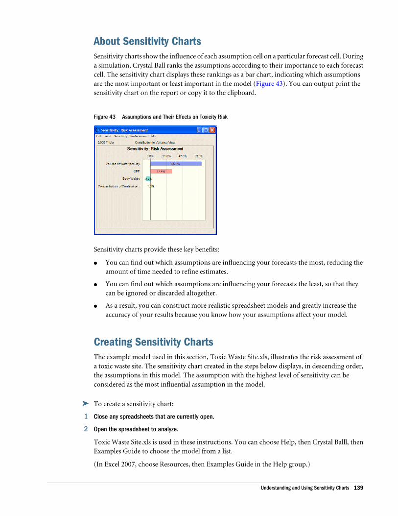
About Sensitivity ChartsSensitivity charts show the influence of each assumption cell on a particular forecast cell. Duringa simulation, Crystal Ball ranks the assumptions according to their importance to each forecastcell. The sensitivity chart displays these rankings as a bar chart, indicating which assumptionsare the most important or least important in the model (Figure 43). You can output print thesensitivity chart on the report or copy it to the clipboard.
Figure 43 Assumptions and Their Effects on Toxicity Risk
Sensitivity charts provide these key benefits:
l You can find out which assumptions are influencing your forecasts the most, reducing theamount of time needed to refine estimates.
l You can find out which assumptions are influencing your forecasts the least, so that theycan be ignored or discarded altogether.
l As a result, you can construct more realistic spreadsheet models and greatly increase theaccuracy of your results because you know how your assumptions affect your model.
Creating Sensitivity ChartsThe example model used in this section, Toxic Waste Site.xls, illustrates the risk assessment ofa toxic waste site. The sensitivity chart created in the steps below displays, in descending order,the assumptions in this model. The assumption with the highest level of sensitivity can beconsidered as the most influential assumption in the model.
ä To create a sensitivity chart:
1 Close any spreadsheets that are currently open.
2 Open the spreadsheet to analyze.
Toxic Waste Site.xls is used in these instructions. You can choose Help, then Crystal Balll, thenExamples Guide to choose the model from a list.
(In Excel 2007, choose Resources, then Examples Guide in the Help group.)
Understanding and Using Sensitivity Charts 139
3 Choose Run, then Run Preferences, then Options.
4 Make sure Store Assumption Values For Sensitivity Analysis is checked and click OK.
Sensitivity analysis requires that all of the random numbers from the simulation be kept forcomparison with forecast values.
5 Run a simulation until it stops.
6 Choose Analyze, then Sensitivity Charts.
(If you are using Crystal Ball in Excel 2007, choose Analyze, then View Charts, then SensitivityCharts.)
The Sensitivity Charts dialog opens. If you have not yet created any sensitivity charts for theactive spreadsheet or restored results file, the dialog is blank.
7 Click the New button.
The Choose Forecast dialog opens.
By default, this dialog opens in a hierarchical Tree view. If you prefer, click the List box to changethe view from a tree to a list. For more information on the Choose Forecast dialog, click the Help
button.
8 Check the box in front of the forecast name to include it in the sensitivity chart.
Toxic Waste.xls has only one forecast, Risk Assessment.
9 Click OK to create a new sensitivity chart as shown in Figure 44.
The illustrated chart has a transparency effect applied using the chart preferences to makesensitivity values easier to read. For instructions, see “Setting Special Chart Effects” on page118.
140 Analyzing Other Charts
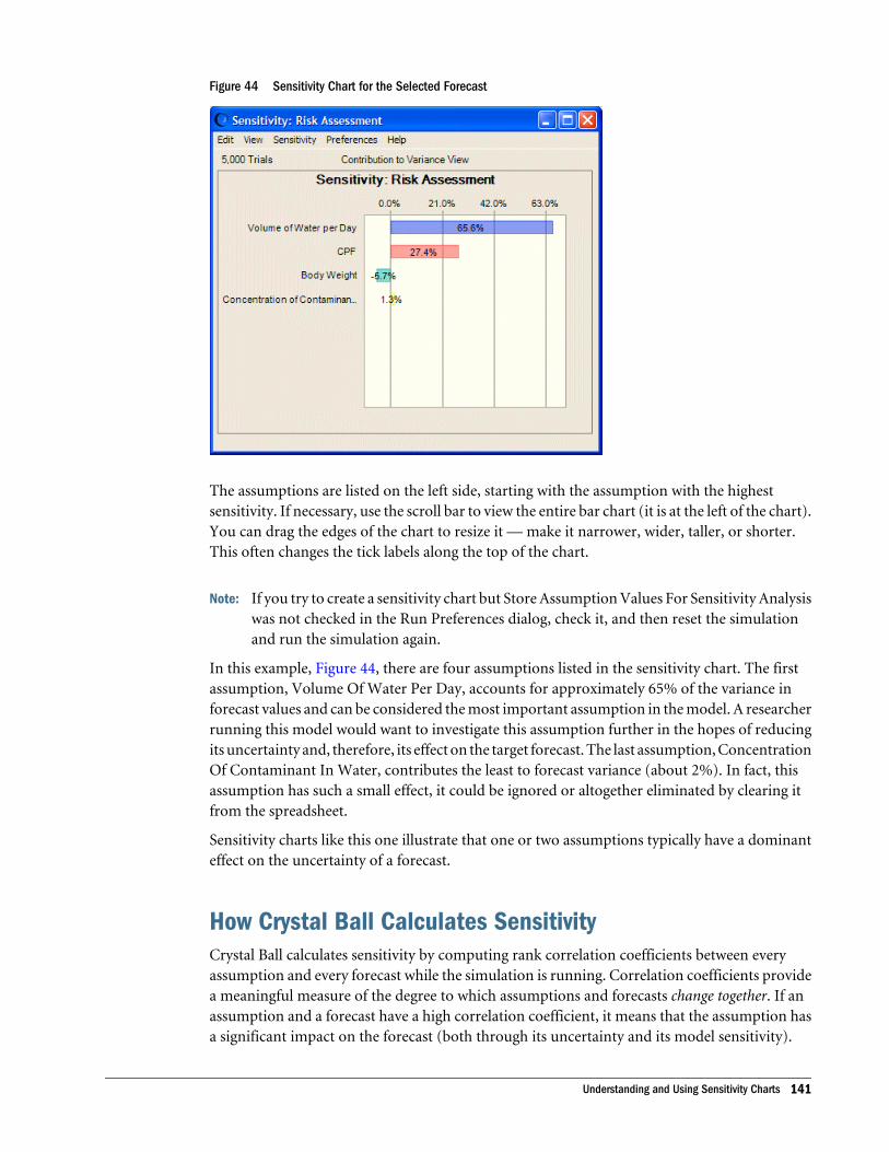
Figure 44 Sensitivity Chart for the Selected Forecast
The assumptions are listed on the left side, starting with the assumption with the highestsensitivity. If necessary, use the scroll bar to view the entire bar chart (it is at the left of the chart).You can drag the edges of the chart to resize it — make it narrower, wider, taller, or shorter.This often changes the tick labels along the top of the chart.
Note: If you try to create a sensitivity chart but Store Assumption Values For Sensitivity Analysiswas not checked in the Run Preferences dialog, check it, and then reset the simulationand run the simulation again.
In this example, Figure 44, there are four assumptions listed in the sensitivity chart. The firstassumption, Volume Of Water Per Day, accounts for approximately 65% of the variance inforecast values and can be considered the most important assumption in the model. A researcherrunning this model would want to investigate this assumption further in the hopes of reducingits uncertainty and, therefore, its effect on the target forecast. The last assumption, ConcentrationOf Contaminant In Water, contributes the least to forecast variance (about 2%). In fact, thisassumption has such a small effect, it could be ignored or altogether eliminated by clearing itfrom the spreadsheet.
Sensitivity charts like this one illustrate that one or two assumptions typically have a dominanteffect on the uncertainty of a forecast.
How Crystal Ball Calculates SensitivityCrystal Ball calculates sensitivity by computing rank correlation coefficients between everyassumption and every forecast while the simulation is running. Correlation coefficients providea meaningful measure of the degree to which assumptions and forecasts change together. If anassumption and a forecast have a high correlation coefficient, it means that the assumption hasa significant impact on the forecast (both through its uncertainty and its model sensitivity).
Understanding and Using Sensitivity Charts 141
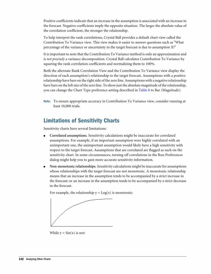
Positive coefficients indicate that an increase in the assumption is associated with an increase inthe forecast. Negative coefficients imply the opposite situation. The larger the absolute value ofthe correlation coefficient, the stronger the relationship.
To help interpret the rank correlations, Crystal Ball provides a default chart view called theContribution To Variance view. This view makes it easier to answer questions such as "Whatpercentage of the variance or uncertainty in the target forecast is due to assumption X?"
It is important to note that the Contribution To Variance method is only an approximation andis not precisely a variance decomposition. Crystal Ball calculates Contribution To Variance bysquaring the rank correlation coefficients and normalizing them to 100%.
Both the alternate Rank Correlation View and the Contribution To Variance view display thedirection of each assumption’s relationship to the target forecast. Assumptions with a positiverelationship have bars on the right side of the zero line. Assumptions with a negative relationshiphave bars on the left size of the zero line. To show just the absolute magnitude of the relationship,you can change the Chart Type preference setting described in Table 8 to Bar (Magnitude).
Note: To ensure appropriate accuracy in Contribution To Variance view, consider running atleast 10,000 trials.
Limitations of Sensitivity ChartsSensitivity charts have several limitations:
l Correlated assumptions. Sensitivity calculations might be inaccurate for correlatedassumptions. For example, if an important assumption were highly correlated with anunimportant one, the unimportant assumption would likely have a high sensitivity withrespect to the target forecast. Assumptions that are correlated are flagged as such on thesensitivity chart. In some circumstances, turning off correlations in the Run Preferencesdialog might help you to gain more accurate sensitivity information.
l Non-monotonic relationships. Sensitivity calculations might be inaccurate for assumptionswhose relationships with the target forecast are not monotonic. A monotonic relationshipmeans that an increase in the assumption tends to be accompanied by a strict increase inthe forecast; or an increase in the assumption tends to be accompanied by a strict decreasein the forecast.
For example, the relationship y = Log(x) is monotonic:
While y = Sin(x) is not:
142 Analyzing Other Charts
The Tornado Chart tool can help you discover if any of your assumptions have non-monotonic relationships with the target forecast. For more information, see “Tornado ChartTool” on page 183.
l Discrete distributions. Sensitivity calculations might be inaccurate for assumptions orforecasts that have a small set of discrete values. Because the sensitivity calculation relies onrank correlation, a slight loss of information occurs when the assumption or forecast valuesare replaced by ranks. This loss of information is generally offset by the advantage of beingable to measure sensitivity between dissimilar types of distributions. However, when a largepercentage of assumption or forecast values are similar or identical, this loss of informationgrows and can significantly distort the calculation of correlations.
Be aware of this problem, for example, for:
m assumptions, when using distributions such as Binomial with a small Trials parameter(for example, < 10).
m forecasts, when formulas in your spreadsheet result in identical values (for example, if-then logic, INT functions, and so on).
Customizing Sensitivity ChartsYou can customize sensitivity charts by changing the assumptions, forecasts, and sensitivitypreferences. As you become more familiar with the sensitivity chart, practice choosing theoptions that help you get the answers you seek and that are appropriate for your data.
The following sections describe how you can customize sensitivity charts:
l “Adding and Removing Assumptions” on page 143
l “Changing the Target Forecast” on page 144
l “Setting Sensitivity Preferences” on page 144
l “Setting Sensitivity Chart Preferences” on page 145
Adding and Removing AssumptionsBy default, the sensitivity chart includes all of the assumptions from the simulation. To removeor change the assumptions included, follow the instructions in this section.
The total number of assumptions included in the chart affects the calculation of the Contributionto Variance percentages.
ä To remove or change assumptions included in the sensitivity chart:
1 In the Sensitivity Chart window, choose Sensitivity, then Choose Assumptions.
Understanding and Using Sensitivity Charts 143
The Choose Assumptions dialog opens.
2 Check the assumptions to add to the sensitivity chart and uncheck those to remove from the chart.
3 Click OK to activate the selected assumptions.
Changing the Target Forecast
ä To change the target forecast in the sensitivity analysis:
1 In the Sensitivity Chart window, choose Sensitivity, then Choose Target Forecast.
The Choose Forecasts dialog opens.
2 Check a new target forecast.
3 Click OK to activate the selected forecast.
Setting Sensitivity PreferencesYou can set a number of preferences that determine:
l The sensitivity view that is displayed
l Whether the sensitivity chart opens automatically and whether it is displayed while thesimulation is running or after it stops
l How many assumptions are shown in the chart, starting with the most sensitive
l Whether sensitivities are limited to a certain sensitivity value or higher
ä To set sensitivity preferences:
1 Choose Preferences, then Sensitivity.
The Sensitivity Preferences dialog opens.
2 To change how the sensitivities are presented, use the View drop-down list:
l Contribution To Variance shows sensitivities as values that range from 0% to 100% andindicate relative importance by showing the percentage of the forecast variance contributedby each assumption.
l Rank Correlation shows sensitivities as rank correlations that range from –1 to +1 andindicate both magnitude and direction of the correlation of each assumption with theforecast.
l Sensitivity Data shows a table of contributions to variance (%) and rank correlations foreach assumption.
3 Use settings in the Windows group to determine whether the chart opens automatically.
If Show Automatically is checked, you can choose whether to display the chart while thesimulation is running or after it stops.
4 To limit sensitivities by rank or value, click the Criteria tab to display it.
144 Analyzing Other Charts
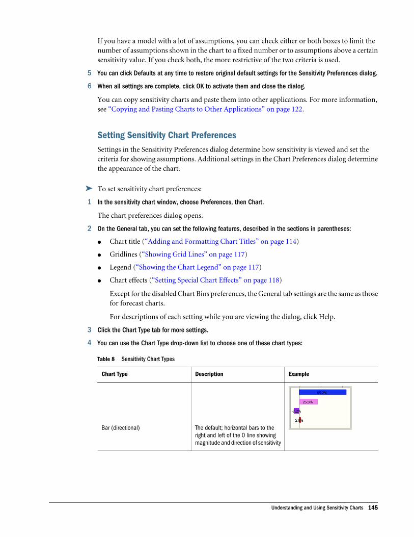
If you have a model with a lot of assumptions, you can check either or both boxes to limit thenumber of assumptions shown in the chart to a fixed number or to assumptions above a certainsensitivity value. If you check both, the more restrictive of the two criteria is used.
5 You can click Defaults at any time to restore original default settings for the Sensitivity Preferences dialog.
6 When all settings are complete, click OK to activate them and close the dialog.
You can copy sensitivity charts and paste them into other applications. For more information,see “Copying and Pasting Charts to Other Applications” on page 122.
Setting Sensitivity Chart PreferencesSettings in the Sensitivity Preferences dialog determine how sensitivity is viewed and set thecriteria for showing assumptions. Additional settings in the Chart Preferences dialog determinethe appearance of the chart.
ä To set sensitivity chart preferences:
1 In the sensitivity chart window, choose Preferences, then Chart.
The chart preferences dialog opens.
2 On the General tab, you can set the following features, described in the sections in parentheses:
l Chart title (“Adding and Formatting Chart Titles” on page 114)
l Gridlines (“Showing Grid Lines” on page 117)
l Legend (“Showing the Chart Legend” on page 117)
l Chart effects (“Setting Special Chart Effects” on page 118)
Except for the disabled Chart Bins preferences, the General tab settings are the same as thosefor forecast charts.
For descriptions of each setting while you are viewing the dialog, click Help.
3 Click the Chart Type tab for more settings.
4 You can use the Chart Type drop-down list to choose one of these chart types:
Table 8 Sensitivity Chart Types
Chart Type Description Example
Bar (directional) The default; horizontal bars to theright and left of the 0 line showingmagnitude and direction of sensitivity
Understanding and Using Sensitivity Charts 145
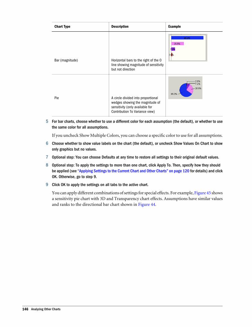
Chart Type Description Example
Bar (magnitude) Horizontal bars to the right of the 0line showing magnitude of sensitivitybut not direction
Pie A circle divided into proportionalwedges showing the magnitude ofsensitivity (only available forContribution To Variance view)
5 For bar charts, choose whether to use a different color for each assumption (the default), or whether to usethe same color for all assumptions.
If you uncheck Show Multiple Colors, you can choose a specific color to use for all assumptions.
6 Choose whether to show value labels on the chart (the default), or uncheck Show Values On Chart to showonly graphics but no values.
7 Optional step: You can choose Defaults at any time to restore all settings to their original default values.
8 Optional step: To apply the settings to more than one chart, click Apply To. Then, specify how they shouldbe applied (see “Applying Settings to the Current Chart and Other Charts” on page 120 for details) and clickOK. Otherwise, go to step 9.
9 Click OK to apply the settings on all tabs to the active chart.
You can apply different combinations of settings for special effects. For example, Figure 45 showsa sensitivity pie chart with 3D and Transparency chart effects. Assumptions have similar valuesand ranks to the directional bar chart shown in Figure 44.
146 Analyzing Other Charts
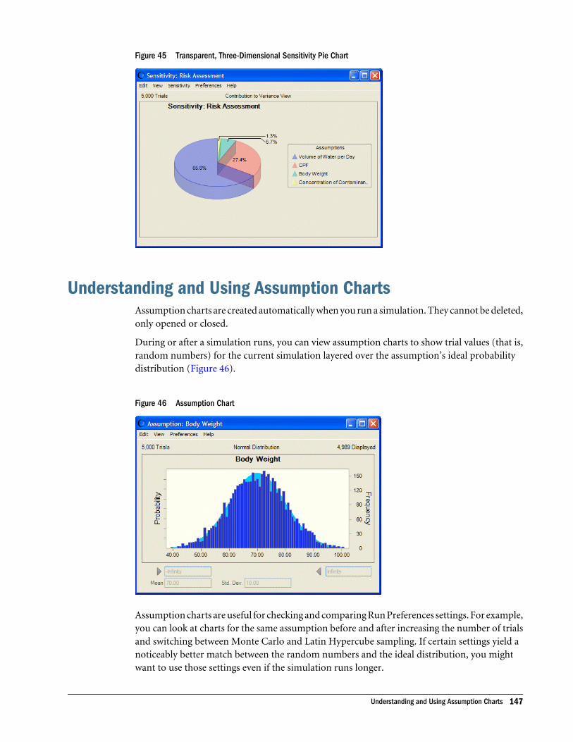
Figure 45 Transparent, Three-Dimensional Sensitivity Pie Chart
Understanding and Using Assumption ChartsAssumption charts are created automatically when you run a simulation. They cannot be deleted,only opened or closed.
During or after a simulation runs, you can view assumption charts to show trial values (that is,random numbers) for the current simulation layered over the assumption’s ideal probabilitydistribution (Figure 46).
Figure 46 Assumption Chart
Assumption charts are useful for checking and comparing Run Preferences settings. For example,you can look at charts for the same assumption before and after increasing the number of trialsand switching between Monte Carlo and Latin Hypercube sampling. If certain settings yield anoticeably better match between the random numbers and the ideal distribution, you mightwant to use those settings even if the simulation runs longer.
Understanding and Using Assumption Charts 147
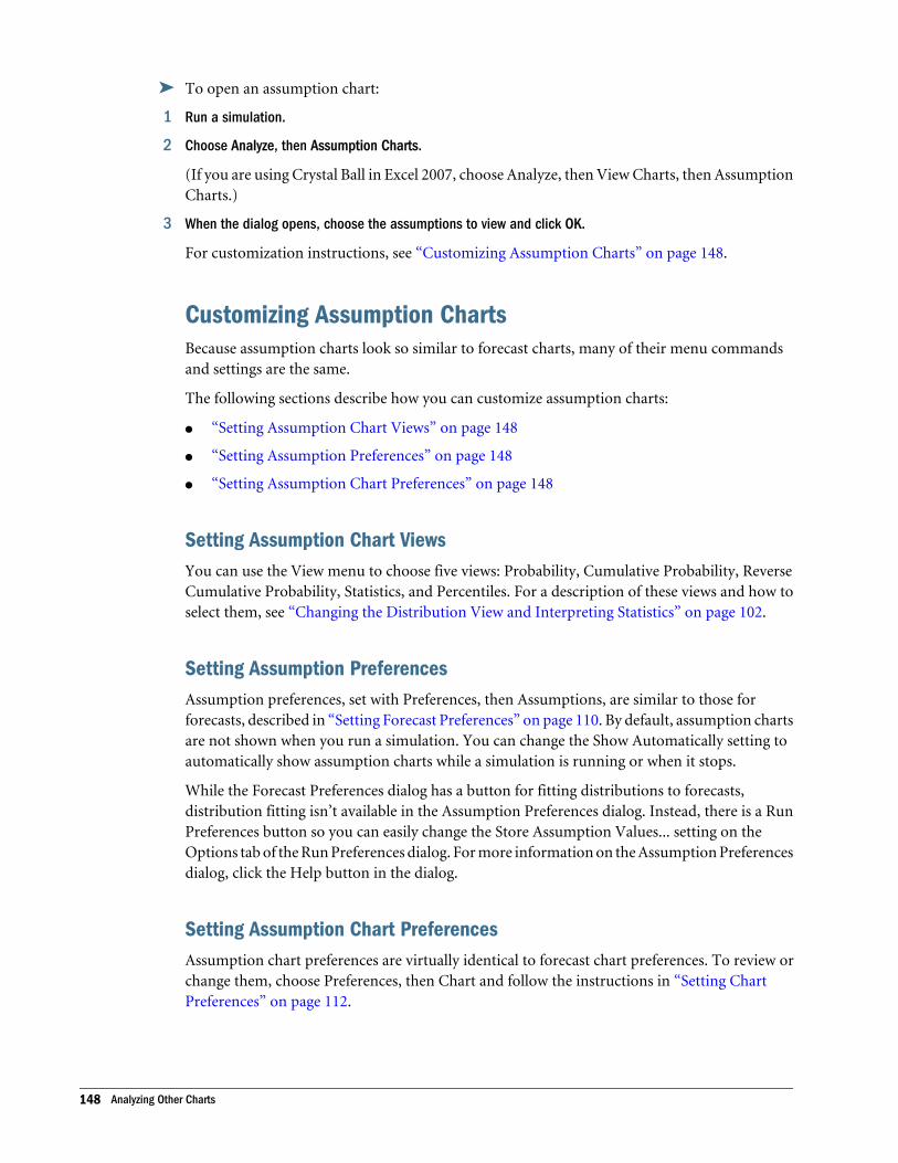
ä To open an assumption chart:
1 Run a simulation.
2 Choose Analyze, then Assumption Charts.
(If you are using Crystal Ball in Excel 2007, choose Analyze, then View Charts, then AssumptionCharts.)
3 When the dialog opens, choose the assumptions to view and click OK.
For customization instructions, see “Customizing Assumption Charts” on page 148.
Customizing Assumption ChartsBecause assumption charts look so similar to forecast charts, many of their menu commandsand settings are the same.
The following sections describe how you can customize assumption charts:
l “Setting Assumption Chart Views” on page 148
l “Setting Assumption Preferences” on page 148
l “Setting Assumption Chart Preferences” on page 148
Setting Assumption Chart ViewsYou can use the View menu to choose five views: Probability, Cumulative Probability, ReverseCumulative Probability, Statistics, and Percentiles. For a description of these views and how toselect them, see “Changing the Distribution View and Interpreting Statistics” on page 102.
Setting Assumption PreferencesAssumption preferences, set with Preferences, then Assumptions, are similar to those forforecasts, described in “Setting Forecast Preferences” on page 110. By default, assumption chartsare not shown when you run a simulation. You can change the Show Automatically setting toautomatically show assumption charts while a simulation is running or when it stops.
While the Forecast Preferences dialog has a button for fitting distributions to forecasts,distribution fitting isn’t available in the Assumption Preferences dialog. Instead, there is a RunPreferences button so you can easily change the Store Assumption Values... setting on theOptions tab of the Run Preferences dialog. For more information on the Assumption Preferencesdialog, click the Help button in the dialog.
Setting Assumption Chart PreferencesAssumption chart preferences are virtually identical to forecast chart preferences. To review orchange them, choose Preferences, then Chart and follow the instructions in “Setting ChartPreferences” on page 112.
148 Analyzing Other Charts
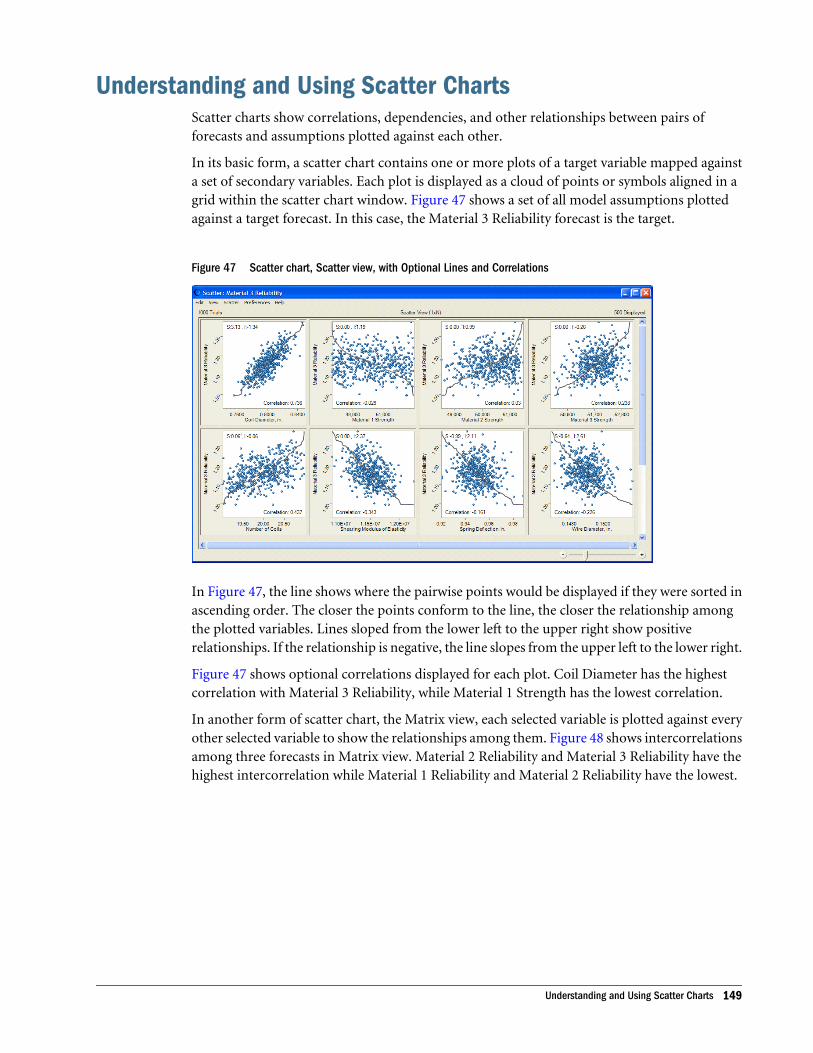
Understanding and Using Scatter ChartsScatter charts show correlations, dependencies, and other relationships between pairs offorecasts and assumptions plotted against each other.
In its basic form, a scatter chart contains one or more plots of a target variable mapped againsta set of secondary variables. Each plot is displayed as a cloud of points or symbols aligned in agrid within the scatter chart window. Figure 47 shows a set of all model assumptions plottedagainst a target forecast. In this case, the Material 3 Reliability forecast is the target.
Figure 47 Scatter chart, Scatter view, with Optional Lines and Correlations
In Figure 47, the line shows where the pairwise points would be displayed if they were sorted inascending order. The closer the points conform to the line, the closer the relationship amongthe plotted variables. Lines sloped from the lower left to the upper right show positiverelationships. If the relationship is negative, the line slopes from the upper left to the lower right.
Figure 47 shows optional correlations displayed for each plot. Coil Diameter has the highestcorrelation with Material 3 Reliability, while Material 1 Strength has the lowest correlation.
In another form of scatter chart, the Matrix view, each selected variable is plotted against everyother selected variable to show the relationships among them. Figure 48 shows intercorrelationsamong three forecasts in Matrix view. Material 2 Reliability and Material 3 Reliability have thehighest intercorrelation while Material 1 Reliability and Material 2 Reliability have the lowest.
Understanding and Using Scatter Charts 149
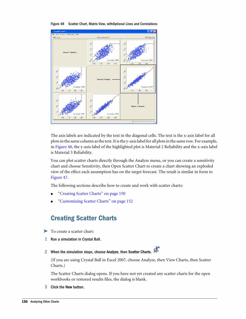
Figure 48 Scatter Chart, Matrix View, withOptional Lines and Correlations
The axis labels are indicated by the text in the diagonal cells. The text is the x-axis label for allplots in the same column as the text. It is the y-axis label for all plots in the same row. For example,in Figure 48, the y-axis label of the highlighted plot is Material 2 Reliability and the x-axis labelis Material 3 Reliability.
You can plot scatter charts directly through the Analyze menu, or you can create a sensitivitychart and choose Sensitivity, then Open Scatter Chart to create a chart showing an explodedview of the effect each assumption has on the target forecast. The result is similar in form toFigure 47.
The following sections describe how to create and work with scatter charts:
l “Creating Scatter Charts” on page 150
l “Customizing Scatter Charts” on page 152
Creating Scatter Charts
ä To create a scatter chart:
1 Run a simulation in Crystal Ball.
2 When the simulation stops, choose Analyze, then Scatter Charts.
(If you are using Crystal Ball in Excel 2007, choose Analyze, then View Charts, then ScatterCharts.)
The Scatter Charts dialog opens. If you have not yet created any scatter charts for the openworkbooks or restored results files, the dialog is blank.
3 Click the New button.
150 Analyzing Other Charts
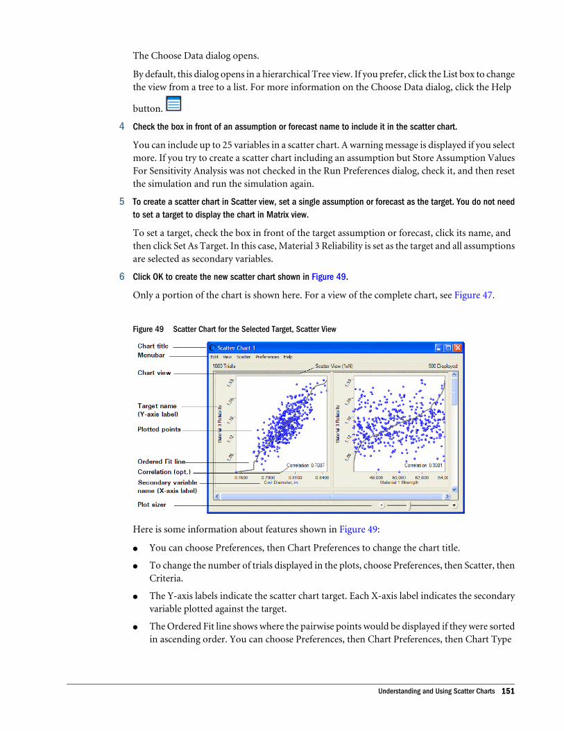
The Choose Data dialog opens.
By default, this dialog opens in a hierarchical Tree view. If you prefer, click the List box to changethe view from a tree to a list. For more information on the Choose Data dialog, click the Help
button.
4 Check the box in front of an assumption or forecast name to include it in the scatter chart.
You can include up to 25 variables in a scatter chart. A warning message is displayed if you selectmore. If you try to create a scatter chart including an assumption but Store Assumption ValuesFor Sensitivity Analysis was not checked in the Run Preferences dialog, check it, and then resetthe simulation and run the simulation again.
5 To create a scatter chart in Scatter view, set a single assumption or forecast as the target. You do not needto set a target to display the chart in Matrix view.
To set a target, check the box in front of the target assumption or forecast, click its name, andthen click Set As Target. In this case, Material 3 Reliability is set as the target and all assumptionsare selected as secondary variables.
6 Click OK to create the new scatter chart shown in Figure 49.
Only a portion of the chart is shown here. For a view of the complete chart, see Figure 47.
Figure 49 Scatter Chart for the Selected Target, Scatter View
Here is some information about features shown in Figure 49:
l You can choose Preferences, then Chart Preferences to change the chart title.
l To change the number of trials displayed in the plots, choose Preferences, then Scatter, thenCriteria.
l The Y-axis labels indicate the scatter chart target. Each X-axis label indicates the secondaryvariable plotted against the target.
l The Ordered Fit line shows where the pairwise points would be displayed if they were sortedin ascending order. You can choose Preferences, then Chart Preferences, then Chart Type
Understanding and Using Scatter Charts 151
to change it to a Linear Regression line, which uses a least-squares technique to show thelinear relationship of the points.
l Auto is the default color for all symbols. With color set to Auto, plots are colored accordingto the combination of variables included in them:
m Assumption vs. assumption = green
m Forecast vs. forecast = dark blue
m Assumption vs. forecast = dark teal (blue-green)
l You can use the Plot Sizer to increase or decrease the size of all plots and the amount ofdetail shown within them. To focus on a single plot, drag the Plot Sizer pointer toward theright to enlarge the plot, and then use the scroll bars to center it.
l In Scatter view, plots move to fill available window space when they are resized. In Matrixview, plots keep the same NxN configuration. You can scroll to view any plots that are notcurrently displayed onscreen.
l Frozen forecasts and assumptions are not included in scatter charts.
Customizing Scatter ChartsYou can customize scatter charts by changing the plotted variables, scatter preferences, and chartpreferences. As you become more familiar with the scatter chart, practice choosing the optionsthat help you get the answers you seek and that are appropriate for your data.
To customize scatter charts, use the menus in the chart window or click portions of the chart:
l Double-click within a plot to open the Chart Preferences dialog.
l Double-click an axis to open the Axis dialog.
l Double-click outside a plot or axis to open the Scatter Preferences dialog.
The following sections describe ways to customize scatter charts:
l “Adding and Removing Assumptions and Forecasts” on page 152
l “Setting Scatter Preferences” on page 153
l “Setting Scatter Chart Preferences” on page 154
l “Scatter Charts and Filtered Data” on page 155
Adding and Removing Assumptions and ForecastsWhen you create a new scatter chart, all assumptions and forecasts in the model are available touse as targets, secondary variables, or matrix variables. Some variables may be closely related tothe target or other elements in the matrix and some variables may be completely unrelated.
You can include up to 25 variables, but scatter charts are easier to interpret with smaller numbersof variables. It can be helpful to edit the chart, removing some secondary variables or matrixelements that show little relationship to each other or a target and adding others that might relatemore closely.
152 Analyzing Other Charts
In complex models with lots of assumptions and forecasts, you might find it helpful to begin bycreating a sensitivity chart and then creating a scatter chart from the data included within it. Forexample, you could open a forecast chart and choose Forecast, then Open Sensitivity Chart toview a sensitivity chart. Then, within the sensitivity chart, you could choose Sensitivity, thenOpen Scatter Chart to create a scatter chart using that forecast as the target.
ä However you create a scatter chart, you can follow these steps to remove or change the variables(forecasts and assumptions) included in it:
1 In the Scatter Chart window, choose Scatter, then Choose Data.
The Choose Data dialog opens.
2 Check the assumptions or forecasts to add to the scatter chart and uncheck those to remove from the chart.
3 If you want, set a different target.
Click the variable name and then click Set As Target.
4 Click OK to display the edited chart.
If you set a new target or remove a target, the view changes when the chart opens again. If youset a new target, the scatter chart is displayed in Scatter view with selected variables plotted againstthe new target. If you remove an existing target and do not set a new one, the chart is displayedin Matrix view.
Setting Scatter PreferencesYou can set a number of preferences that determine:
l The scatter view that is displayed
l Whether the scatter chart opens automatically and whether it is displayed while thesimulation is running or after it stops
l The plot size
l The number of trials that are plotted relative to the total number of trials in each simulation
ä To set scatter preferences:
1 Choose Preferences, then Scatter.
The Scatter Preferences dialog opens.
2 To change how the scatter chart is presented, use the View drop-down list:
l Scatter View (1xN) shows secondary variables plotted against a target.
l Matrix View (NxN) shows all selected variables plotted against each other.
3 Use settings in the Window group to determine whether the chart opens automatically.
If Show Automatically is checked, you can choose whether to display the chart while thesimulation is running or after it stops.
4 To change the size and amount of detail shown in each plot, use the Plot Sizer.
Understanding and Using Scatter Charts 153
Slide it left to decrease or right to increase plot size. To set the new size as a global default orapply it to other scatter charts, click Apply To and choose appropriate settings. Click Help foradditional information.
5 To determine the number of trials that are plotted relative to the total number of trials in each simulation,click the Criteria tab to display it.
By default, only a portion of trials are plotted for each simulation, based on the total number oftrials. To display all trials or a specific number, choose Show The First ____ Trials and enter thenumber of trials to display. Or, you can choose Show The First ___% Of The Trials to show acertain percent of the trials, from 1% to 100%.
6 You can click Defaults at any time to restore original default settings for the Scatter Preferences dialog orclick Apply To to set new defaults.
7 When all settings are complete, click OK to activate them and close the dialog.
You can copy scatter charts and paste them into other applications. For more information, see“Copying and Pasting Charts to Other Applications” on page 122.
Setting Scatter Chart PreferencesSettings in the Scatter Preferences dialog determine which scatter chart view is displayed and setthe criteria for plotting all or a portion of trials actually run. Additional settings in the ChartPreferences dialog determine the appearance of the chart.
ä To set scatter chart preferences:
1 In the scatter chart window, choose Preferences, then Chart.
The Chart Preferences dialog opens.
2 On the General tab, you can set the following features, described in the sections in parentheses:
l Chart title (“Adding and Formatting Chart Titles” on page 114)
l Gridlines (“Showing Grid Lines” on page 117)
l Legend (“Showing the Chart Legend” on page 117)
l Chart effects (“Setting Special Chart Effects” on page 118)
Except for the disabled Chart Bins and 3D Chart preferences, the General tab settings arethe same as those for forecast charts.
For descriptions of each setting while you are viewing the dialog, click Help.
3 Click the Chart Type tab for more settings.
4 You can use the Chart Type drop-down list to choose whether to:
l Draw points, and if selected, to choose a symbol, color, and size for them.
l Draw a line, and if selected, to choose a line type, color and size. The Ordered Fit line typeshows where pairwise points would be displayed if they were sorted in ascending order. TheLinear Regression line type uses a least-squares technique to show the linear relationship ofthe points.
154 Analyzing Other Charts
l Display correlation coefficients for each plot. These are computed using the Spearman rankcorrelation method.
l Display points that have been filtered out (see the next section, “Scatter Charts and FilteredData” on page 155).
5 You can use the Axis tab to choose a number format for the chart axes and to indicate whether to round axisvalues, as described in “Customizing Chart Axes and Axis Labels” on page 120.
6 Optional step: You can choose Defaults at any time to restore all settings to their original default values.
7 Optional step: To apply the settings to more than one chart, click Apply To. Then, specify how they shouldbe applied (see “Applying Settings to the Current Chart and Other Charts” on page 120 for details) and clickOK. Otherwise, go to step 7.
8 Click OK to apply the settings on all tabs to the active chart.
Scatter Charts and Filtered DataYou can use the Filter tab of the Forecast Preferences dialog to include or exclude specific rangesof data from forecast charts (“Filter Tab” on page 67). If you include a filtered forecast in a scatterchart, you can choose whether or not to show filtered points in the chart.
ä To change this setting:
1 Open the scatter chart and choose Preferences, then Chart.
2 Click the Chart Type tab.
3 Check or uncheck Show Points That Have Been Filtered Out to show or hide the filtered points, respectively.
4 Click OK.
By default, filtered points are displayed in scatter charts as very light (grayed) points or symbols.
Figure 50 shows the same data as Figure 47 except Material 3 Reliability has been filtered to onlyinclude data between 1.08 and 1.23. Excluded data shows as very light triangles while includeddata is plotted normally, in this case as transparent blue triangles, size 4.
Understanding and Using Scatter Charts 155
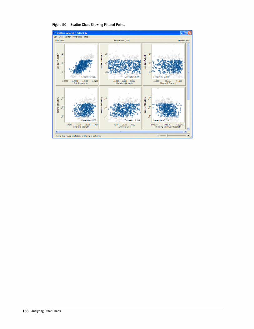
Figure 50 Scatter Chart Showing Filtered Points
156 Analyzing Other Charts
8Creating Reports and Extracting
Data
In This Chapter
Introduction... . . . . . . . . . . . . . . . . . . . . . . . . . . . . . . . . . . . . . . . . . . . . . . . . . . . . . . . . . . . . . . . . . . . . . . . . . . . . . . . . . . . . . . . . . . . . . . . . . . . . . . . . . . . . . . . . . . . . 157
Creating Reports .. . . . . . . . . . . . . . . . . . . . . . . . . . . . . . . . . . . . . . . . . . . . . . . . . . . . . . . . . . . . . . . . . . . . . . . . . . . . . . . . . . . . . . . . . . . . . . . . . . . . . . . . . . . . . . . . 157
Extracting Data ... . . . . . . . . . . . . . . . . . . . . . . . . . . . . . . . . . . . . . . . . . . . . . . . . . . . . . . . . . . . . . . . . . . . . . . . . . . . . . . . . . . . . . . . . . . . . . . . . . . . . . . . . . . . . . . . . 161
IntroductionThis chapter describes how to create reports with charts and data and how to extract data foruse in other applications.
See the following sections for instructions:
l “Creating Reports” on page 157
l “Extracting Data” on page 161
Creating ReportsYou can generate pre-defined reports for your simulation or you can create a custom report withany or all of the following items:
l Report summary
l Forecasts
l Assumptions
l Decision variables
l Overlay charts
l Trend charts
l Sensitivity charts
l Scatter charts
Figure 51 shows part of a forecast report for the Vision Research model.
Introduction 157
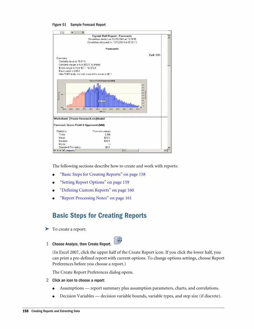
Figure 51 Sample Forecast Report
The following sections describe how to create and work with reports:
l “Basic Steps for Creating Reports” on page 158
l “Setting Report Options” on page 159
l “Defining Custom Reports” on page 160
l “Report Processing Notes” on page 161
Basic Steps for Creating Reports
ä To create a report:
1 Choose Analyze, then Create Report.
(In Excel 2007, click the upper half of the Create Report icon. If you click the lower half, youcan print a pre-defined report with current options. To change options settings, choose ReportPreferences before you choose a report.)
The Create Report Preferences dialog opens.
2 Click an icon to choose a report:
l Assumptions — report summary plus assumption parameters, charts, and correlations.
l Decision Variables — decision variable bounds, variable types, and step size (if discrete).
158 Creating Reports and Extracting Data
l Forecasts — report summary plus forecast summaries, charts, statistics, percentiles, andcapability metrics if generated.
l Full, the default — all sections and details except assumption statistics and percentiles.
l Index — only forecast, assumption, and decision variable summaries.
l Custom — displays the Custom Report dialog for report definition.
l OptQuest — if you have OptQuest and have active optimization data, displays OptQuestresults.
l Predictor — if you have run Predictor and have active time series forecast data, displaysPredictor results.
3 If you choose Custom, click the Custom button and complete the Custom Report dialog (“Defining CustomReports” on page 160). Otherwise, continue with step 4.
4 Click the Options tab to set a location and format for the report (“Setting Report Options” on page 159).
(In Excel 2007, if you clicked the lower half of the Create Report icon, choose Report Preferencesto set a location and format for the report before you choose a report.)
5 When all settings are complete, click OK.
Crystal Ball creates the report as an Excel worksheet. You can modify, print, or save the reportin the same way as any other worksheet. For example, you can choose the File, then Print optionfor your spreadsheet model as you would for a normal spreadsheet.
Note: If ### is displayed in your report instead of a numeric value, try making the column widerto show the entire number.
Setting Report OptionsReport options specify the report location and format.
ä To set report options:
1 In the Create Report dialog, click the Options tab.
(In Excel 2007, if you clicked the lower half of the Create Report icon, choose Report Preferencesto set a location and format for the report before you choose a report.)
2 In the Location group, choose whether to create the report in a new Excel workbook or the current workbook.
If you choose Current Workbook, a new sheet is created right after the current sheet. You canenter a descriptive name for the new sheet in the Sheet Name field.
3 In the Formatting group, indicate whether to include the cell location (workbook, worksheet, and cell address)in the rightmost column of report headers and whether to include cell comments.
By default, these settings are checked.
If you choose to include cell comments, only non-Crystal Ball comments are included; CrystalBall cell comments are redundant and are filtered out.
Creating Reports 159
4 In the Chart Format group, choose Image to create a Crystal Ball chart or choose Excel to create an Excelchart.
If you choose Image, you can format charts using the Crystal Ball Chart Preference settings.Image is the default chart format.
5 When all settings are complete, click OK.
Defining Custom Reports
ä To define a custom report:
1 Follow the steps in “Basic Steps for Creating Reports” on page 158 to display the Create Report dialog.
2 Click the Custom button.
3 In the Custom Report dialog, check one or more items in the Report Sections group to include in the report:
l Report Summary — The report title, date and time, Run Preferences settings, and runstatistics.
l Forecasts — Forecast information, including the name, charts, percentiles, statistics, andmore.
l Assumptions — Assumption information, including parameters, charts, percentiles,statistics, and correlations.
l Decision Variables — Decision variable information, including type (continuous ordiscrete) with step if discrete, plus lower and upper bounds.
l Charts (Overlay, Trend, Sensitivity, Scatter, OptQuest) — Includes the selected type ofchart(s) in the report. You can scale the size of the charts by entering a percentage in thefield.
Note: Excel charts cannot be created for assumptions defined as custom distributions.
If you have activated the process capability features and have generated capability metrics,you can include them in your custom report (“Including Capability Metrics in Reports” onpage 392).
4 As each item is highlighted in the Report Sections group, check appropriate settings in the Details group:
l Report Summary: Report Title, Date/Time, Run Preferences (Run Preferences settings forthe report), Run Statistics
l Forecasts: Summary, Chart And Size, Statistics, Percentiles, Parameters
l Assumptions: Chart And Size, Statistics, Percentiles, Correlations
l Decision Variables: Type, Step Size, Bounds
l Overlay Charts: Chart And Size
l Trend Charts: Chart And Size
l Sensitivity Charts: Chart And Size
160 Creating Reports and Extracting Data
l Scatter Charts: Chart And Size
l OptQuest Charts: Chart And Size
l Predictor Charts: Chart And Size
When no details are selected for a custom report section, only a single row is output withthe Crystal Ball item name and the cell reference.
5 For each item checked in Report Sections, choose whether to display all of that type of item, only selecteditems, or all open items. If you select Choose, a dialog opens so you can check the box in front of each itemto display.
6 When these settings are complete, click OK to close the dialog and return to the Create Report dialog.
7 In the Create Report dialog, click the Options tab to display it (“Setting Report Options” on page 159).
8 When all the report options are set, click OK to close the dialog and create the report.
Report Processing NotesThe following are special notes concerning Crystal Ball reports:
l No section is created if there are no Crystal Ball items for that section.
l Statistics follow the chart by default.
l The Choose, then All options always include restored results if they exist.
l If scroll bars are present in a chart, they are displayed in the report.
l If an assumption has been truncated, you might want to add marker lines to show wherethe distribution has been truncated. To do this, display the Chart Type tab in the ChartPreferences dialog and set an appropriate Value marker.
l Sensitivity Charts and Scatter Charts in Scatter view include only the portion of those chartsavailable onscreen at the time the report is requested.
Extracting DataYou can extract assumption and forecast information generated during a Crystal Ball simulation.Crystal Ball places the extracted data in the specified worksheet location. You can only extractdata after you run a simulation or restore saved results.
ä To extract data:
1 Choose Analyze, then Extract Data.
The Extract Data dialog opens.
2 To select the type of data to extract, choose the appropriate setting in the Select Data To Extract list:
l Statistics — Descriptive statistics summarizing the assumption and forecast values.
Extracting Data 161
l Percentiles — The probability of achieving values below a particular threshold in the selectedincrements. Note: You can reverse the meaning of the percentiles by changing the setting inthe Run Preferences, then Options panel (“Setting Statistics Preferences” on page 80).
l Chart Bins — For each group interval, or bin, the interval range as well as the probabilityand frequency of occurrences within the interval for the forecast. This setting is independentof the Chart Preferences density setting that controls how many bins or data points aredisplayed in a graphic chart.
l Sensitivity Data — Sensitivity data (such as the rank correlation coefficient) for all pairs ofassumptions and forecasts indicating the strength of the relationship. If you plan to extractsensitivity data, be sure to check Store Assumption Values For Sensitivity Analysis on theOptions tab of the Run Preferences dialog (“Setting Options Preferences” on page 79).Note: Data is extracted for all assumptions regardless of assumptions selected for extraction.
l Trial Values — The generated assumption and forecast values for each simulation trial.
l Capability Metrics — Process capability metric values, if available. If you have activated theprocess capability features and have generated capability metrics, you can extract them(“Extracting Capability Metrics” on page 391).
If you choose Percentiles or Chart Bins, a dialog opens so you can choose which percentilesor how many bins to use. Choose Custom and enter a set of custom percentiles if the set youneed is not already available in the dialog.
Data types are extracted in the order they are displayed in the Select Data To Extract list.You can use the up and down arrows to rearrange the data types.
3 In the Forecasts group, select forecasts for data extraction (All, Choose, or None):
l To include the selected data and restored results for all forecasts in the current simulation,choose All.
l To include the selected data for only selected forecasts or to include forecasts in selectedrestored results files, choose Choose.
l Choose None if you don’t want to extract any forecast data.
If you choose Choose, the Choose Forecasts dialog opens.
Only forecasts for which data was generated or restored are included in the list. Any restoredresults are displayed after current data and have file names with the .cbr extension.
By default, the Choose Forecasts dialog is in a hierarchical Tree view. You can click the List
button at the top to change it to List view.
4 In the Assumptions group, select assumptions for data extraction (All, Choose, or None):
l To include the selected data for all assumptions and restored results in the currentsimulation, choose All.
l To include the selected data for only selected assumptions or to include assumptions inselected restored results files, choose Choose.
The Choose Assumptions dialog opens so you can choose from list of available assumptions.It works similarly to the Choose Forecasts dialog, described previously. For moreinformation on the Choose Assumptions dialog, click the Help button.
162 Creating Reports and Extracting Data

l Choose None if you don’t want to extract any assumption data.
You can only extract data for calculated assumption values using the Extract Data command.To view statistics for theoretical data, display an assumption chart and then choose View,then Statistics.
5 If you have active OptQuest or Predictor data, make appropriate settings to extract the target data. For details,see the Crystal Ball Decision Optimizer OptQuest User's Guide or the Crystal Ball Predictor User's Guide.
6 Click the Options tab to specify a location or formatting for the extracted data.
7 In the Location area of the Options tab:
l To extract data to a new workbook, choose New Workbook.
l To extract data to a new worksheet in the active workbook, choose Current Workbook, thenNew Sheet.
l To extract data to the current sheet, choose Current Workbook, then Current Sheet.
8 Specify the name of the sheet and the first cell of the range where the extracted data will be stored.
9 Check settings in the Formatting group to indicate how to format the extracted data:
l When checked, Include Labels adds row and column headers to the data table. Otherwise,just the numeric values are extracted.
l When checked, Include Cell Locations adds the workbook, worksheet, and cell address abovethe object name in the column header. Otherwise, only the object name is displayed.
l When checked, AutoFormat applies the following formats to extracted data:
m Bold font for column headers
m Border beside row labels
m Border beneath column headers
m Border before first assumption
m Numeric formatting to values
m AutoFit width to columns
10 You can click the Defaults button at any time to restore the original settings to both tabs of the Extract Datadialog.
11 When both the Data and Options tab settings are complete, click OK.
Crystal Ball extracts the simulation data to the specified worksheet location. The extracted datais arranged as columns of forecasts and assumptions and rows of data. You can sort, modify,print, or save the data in the same way as any other spreadsheet.
For examples of extracted data, see “Data Extraction Examples” on page 164.
Extracting Data 163
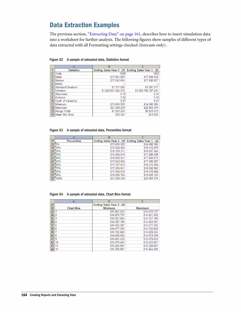
Data Extraction ExamplesThe previous section, “Extracting Data” on page 161, describes how to insert simulation datainto a worksheet for further analysis. The following figures show samples of different types ofdata extracted with all Formatting settings checked (forecasts only).
Figure 52 A sample of extracted data, Statistics format
Figure 53 A sample of extracted data, Percentiles format
Figure 54 A sample of extracted data, Chart Bins format
164 Creating Reports and Extracting Data
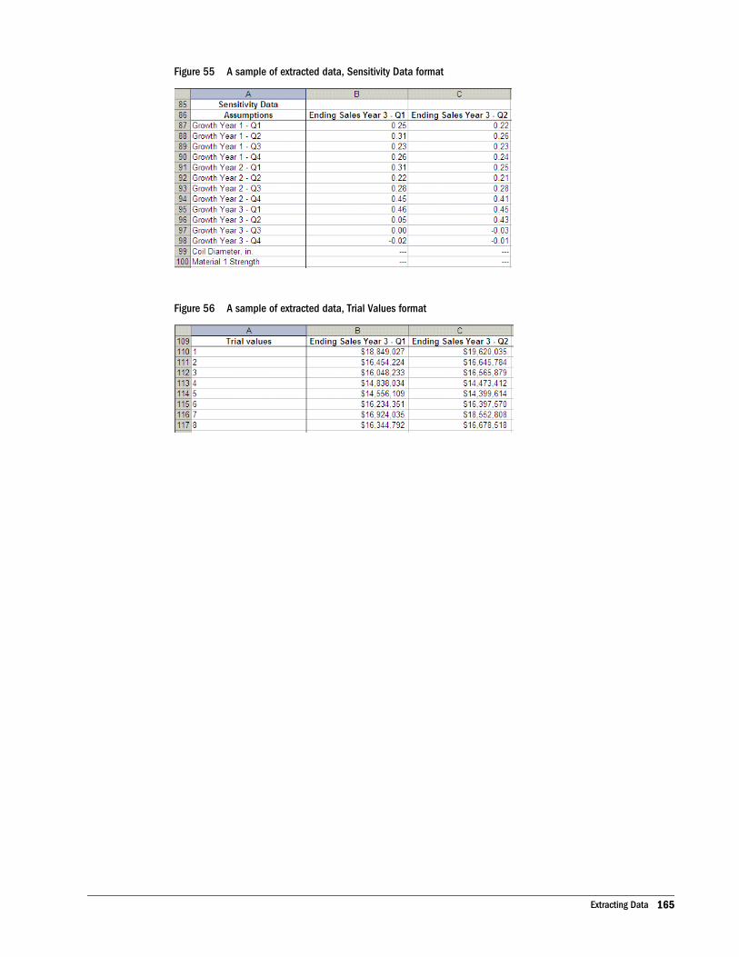
Figure 55 A sample of extracted data, Sensitivity Data format
Figure 56 A sample of extracted data, Trial Values format
Extracting Data 165

166 Creating Reports and Extracting Data
9Crystal Ball Tools
In This Chapter
Introduction... . . . . . . . . . . . . . . . . . . . . . . . . . . . . . . . . . . . . . . . . . . . . . . . . . . . . . . . . . . . . . . . . . . . . . . . . . . . . . . . . . . . . . . . . . . . . . . . . . . . . . . . . . . . . . . . . . . . . 167
Overview ... . . . . . . . . . . . . . . . . . . . . . . . . . . . . . . . . . . . . . . . . . . . . . . . . . . . . . . . . . . . . . . . . . . . . . . . . . . . . . . . . . . . . . . . . . . . . . . . . . . . . . . . . . . . . . . . . . . . . . . . 167
Batch Fit Tool .. . . . . . . . . . . . . . . . . . . . . . . . . . . . . . . . . . . . . . . . . . . . . . . . . . . . . . . . . . . . . . . . . . . . . . . . . . . . . . . . . . . . . . . . . . . . . . . . . . . . . . . . . . . . . . . . . . . . 169
Correlation Matrix Tool.. . . . . . . . . . . . . . . . . . . . . . . . . . . . . . . . . . . . . . . . . . . . . . . . . . . . . . . . . . . . . . . . . . . . . . . . . . . . . . . . . . . . . . . . . . . . . . . . . . . . . . . . . . 177
Tornado Chart Tool .. . . . . . . . . . . . . . . . . . . . . . . . . . . . . . . . . . . . . . . . . . . . . . . . . . . . . . . . . . . . . . . . . . . . . . . . . . . . . . . . . . . . . . . . . . . . . . . . . . . . . . . . . . . . . . 183
Bootstrap Tool .. . . . . . . . . . . . . . . . . . . . . . . . . . . . . . . . . . . . . . . . . . . . . . . . . . . . . . . . . . . . . . . . . . . . . . . . . . . . . . . . . . . . . . . . . . . . . . . . . . . . . . . . . . . . . . . . . . . 191
Decision Table Tool .. . . . . . . . . . . . . . . . . . . . . . . . . . . . . . . . . . . . . . . . . . . . . . . . . . . . . . . . . . . . . . . . . . . . . . . . . . . . . . . . . . . . . . . . . . . . . . . . . . . . . . . . . . . . . 199
Scenario Analysis Tool.. . . . . . . . . . . . . . . . . . . . . . . . . . . . . . . . . . . . . . . . . . . . . . . . . . . . . . . . . . . . . . . . . . . . . . . . . . . . . . . . . . . . . . . . . . . . . . . . . . . . . . . . . . 205
2D Simulation Tool .. . . . . . . . . . . . . . . . . . . . . . . . . . . . . . . . . . . . . . . . . . . . . . . . . . . . . . . . . . . . . . . . . . . . . . . . . . . . . . . . . . . . . . . . . . . . . . . . . . . . . . . . . . . . . 210
Data Analysis Tool .. . . . . . . . . . . . . . . . . . . . . . . . . . . . . . . . . . . . . . . . . . . . . . . . . . . . . . . . . . . . . . . . . . . . . . . . . . . . . . . . . . . . . . . . . . . . . . . . . . . . . . . . . . . . . . 219
IntroductionThis chapter describes the Crystal Ball tools. For each tool, there is a general description, atutorial, and references to descriptions of all panels, fields, and options.
In addition, see “Numerical Differences and the Compare Run Modes Tool” on page 318 forinformation about the Compare Run Modes tool, used to determine how much faster yourmodel could run with Extreme Speed, if you have Crystal Ball Decision Optimizer.
OverviewCrystal Ball tools are features in the Run, then More Tools menu that extend the functionalityof Crystal Ball. They cover two aspects of Crystal Ball modeling plus integration with other Oracleproducts:
l “Setup Tools” on page 168
l “Analysis Tools” on page 168
l “Integration Tools” on page 168
This chapter describes each tool and provides a step-by-step example for using it.
Introduction 167
Note: Some of the tools can take a long time to run. Should you need to cancel a tool before itstops by itself, click in the Excel window and hit Esc. A panel opens and you can chooseto End or Continue.
Setup ToolsThe following are Crystal Ball setup tools, described in the referenced sections:
l “Batch Fit Tool” on page 169 — Automatically fits selected probability distributions tomultiple data series.
l “Correlation Matrix Tool” on page 177 — Rapidly defines and automates correlations ofassumptions.
l “Tornado Chart Tool” on page 183 — Individually analyzes the impact of each modelvariable on a target outcome.
Analysis ToolsThe following are Crystal Ball analysis tools, described in the referenced sections:
l “Bootstrap Tool” on page 191 — Addresses the reliability and accuracy of forecast statistics.
l “Decision Table Tool” on page 199 — Evaluates the effects of alternate decisions in asimulation model.
l “Scenario Analysis Tool” on page 205 — Displays what inputs created particular outputs.
l “2D Simulation Tool” on page 210 — Independently addresses uncertainty and variabilityusing a two-dimensional simulation.
l “Data Analysis Tool” on page 219 — Imports one or more series of raw data and performsa variety of analyses on them.
Integration ToolsThe integration tools, available with Crystal Ball EPM, enable you to run Crystal Ball simulationsagainst Oracle Hyperion Strategic Finance, Fusion Edition and other Oracle EnterprisePerformance Management products such as Oracle Essbase working through Oracle HyperionSmart View for Office, Fusion Edition. For information about the Crystal Ball DecisionOptimizer Strategic Finance and Enterprise Performance Management integration tools, see theOracle Crystal Ball Enterprise Performance Management, Fusion Edition Integration Guide.
Tools and Run PreferencesFor consistency from one run to the other, it can be helpful to choose Latin Hypercube samplingon the Sampling tab of the Run Preferences dialog. You can also choose to use the same sequenceof random numbers with a specific random seed value. The default is 999.
168 Crystal Ball Tools

Note: If you do not set a random seed value before running one of the Crystal Ball tools, CrystalBall will set a value for you and will notify you of this when you run a tool.
Batch Fit ToolThe Batch Fit tool fits probability distributions to multiple data series. You can select any or allof the probability distributions (binomial, normal, triangular, uniform, and so on) to fit to anynumber of series limited only by the size of your spreadsheet.
Batch Fit is intended to help you create assumptions when you have historical data for severalvariables. It selects which distribution best fits each series of historical data, and gives you thedistribution and its associated parameters for you to use in your model. This tool also gives youa table of goodness-of-fit statistics for the best fitting distribution and provides a matrix ofcorrelations calculated between multiple data series so you can easily see which series are relatedand to what degree.
To use the Batch Fit tool, your data series must be contiguous (in adjacent rows or columns) ineither rows or columns.
You can select any combination of probability distributions to fit to all your data series.
Using the Batch Fit ToolTo use the Batch Fit tool, you start it and then use the wizard panels to define inputs and outputs,set options, and run the tool.
Topics in this section include:
l “Starting the Batch Fit Tool” on page 169
l “Using the Batch Fit Welcome Panel” on page 170
l “Setting Batch Fit Input Data Options” on page 170
l “Setting Batch Fit Fitting Options” on page 170
l “Setting Batch Fit Output Options” on page 171
Also see “Batch Fit Example” on page 172.
Starting the Batch Fit Tool
ä To start the Batch Fit tool:
1 In Excel with Crystal Ball loaded, open or build the workbook to analyze.
2 Select Run, then More Tools, then Batch Fit. (In Microsoft Excel 2007, select More Tools in the Tools group.)
If this is the first time you have opened the Batch Fit tool, the Welcome panel opens.
Batch Fit Tool 169
Using the Batch Fit Welcome PanelThe Welcome panel opens the first time you use the Batch Fit tool. It describes the tool and itsuse. The controls for this panel are:
l Next — Opens the Input Data panel for specifying the location of the data series.
l Run — Runs the Batch Fit tool.
ä To continue with the Batch Fit tool, click Next.
The Input Data panel opens.
Setting Batch Fit Input Data OptionsThe Input Data panel of the Batch Fit wizard indicates the location of the data to fit to thedistributions selected in the next panel. You can also specify other input-related options.
When you open this panel, the Batch Fit data selector chooses possible data for fitting. Thisinformation is displayed in the Location Of Data Series field and the illustration at the right sideof the panel. You can choose different data if necessary. The fields and options in this panel are:
l Location Of Data Series — Used to enter or interactively select the cells that contain data tofit. If your data has headers or labels at the beginning of the rows or columns of data, includethem in your selection and select the appropriate Headers setting(s). The data must be inadjacent rows or columns.
l Orientation — Indicates whether your data is in rows or columns. Data In Rows indicatesthat data is in horizontal rows. Data In Columns indicates that data is in vertical columns.
l Headers — Indicates whether your data has headers and/or labels and whether they arelocated in the top row or the left header (varies with orientation). Checked items are usedin the output. Top Row Has Headers/Labels, when checked, includes text in the top row inyour selection. Left Column Has Labels/Headers, when checked, includes text in the leftcolumn in your selection.
l Back — Returns to the Welcome panel.
l Next — Advances to the Fitting Options panel.
l Run — Runs the tool, automatically fitting distributions to your data and creating outputof the assumptions and statistics.
ä When all Input Data settings are complete, click Next to open the Fitting Options panel.
Setting Batch Fit Fitting OptionsThe Fitting Options panel of the Batch Fit wizard indicates which distributions to fit to each setof data. The Fitting Options panel has these settings:
l Distributions To Fit — Indicates the distributions to use for fitting:
m AutoSelect — Crystal Ball chooses the best type of distribution for fitting
170 Crystal Ball Tools
m All Continuous — Fits the data to all those distributions in which every value in thedistribution’s range is possible (these distributions are displayed as solid shapes on theDistribution Gallery)
m All Discrete — Fits the data to all discrete (non-continuous) distributions in theDistribution Gallery (except Yes-No)
m Choose — Displays another dialog from which you can select a subset of thedistributions to include in the fitting.
l Rank By Goodness-of-Fit Statistic — Indicates which ranking method to use for determiningthe best fit:
m AutoSelect — Crystal Ball chooses the best available goodness-of-fit statistic to use forranking.
m Anderson-Darling — Closely resembles the Kolmogorov-Smirnov method, except thatit weights the differences between the two distributions at their tails greater than at theirmid-ranges; use this method when you need a better fit at the extreme tails of thedistribution.
m Chi-Square — Oldest and most common of the goodness-of-fit tests; gauges the generalaccuracy of the fit by breaking down the distribution into areas of equal probability andcomparing the data points within each area to the number of expected data points.
m Kolmogorov-Smirnov — Finds the largest vertical distance between the two cumulativedistributions.
l Lock Parameters — When you check this box or click the Ellipsis (...) button, opens theLock Parameters dialog, where you can choose parameters to lock during fitting and specifytheir values.
Note: If you know location, shape, or other parameter values that might help create a moreaccurate fit with certain distributions, check Lock Parameters and enter appropriatevalues in the Lock Parameters dialog. For details, see “Locking Parameters WhenFitting Distributions” on page 47.
l Back — Returns to the Input Data panel.
l Next — Opens the Output Options panel.
l Run — Runs the tool, automatically fitting distributions to your data and creating outputof the assumptions and statistics.
ä When all Fitting Options settings are complete, click Next to open the Output Options panel.
Setting Batch Fit Output OptionsThe Output Options panel of the Batch Fit wizard sets output options that control the tool.Available settings and buttons are:
l Fit Results (Assumptions), Locations — Specifies locations of results:
m New Workbook — Places results in a new workbook.
Batch Fit Tool 171
m Current Workbook — Places results in the current workbook. You can choose NewSheet, which places results in a new sheet of the current workbook, or Current Sheet,which places results in an existing sheet of the current workbook; you can specify theleft corner of the output range (results are displayed to the right and downward fromthat cell).
l Fit Results (Assumptions), Format Output — When checked, uses special cell formattingfor your data in your output.
l Correlations — Specifies whether correlations are generated and defined:
m Show Correlation Matrix Between Data Series — When checked, correlates the dataseries with each other and displays the results in a matrix.
m Define Correlations Between Assumptions If The Absolute Value Of The CorrelationIs Above __ — When checked, defines correlations between assumptions if the absolutevalue of the correlation is above the indicated level. The default is 0.0, whichintercorrelates all assumptions.
m Keep Correlations Linked To Matrix — When checked, changes correlations betweenassumptions if a new matrix is generated.
l Reports — Indicates which reports to generate and their sheet names:
m Create Goodness-Of-Fit Report — When checked, creates a goodness-of-fit report ona separate worksheet with the specified name.
m Show All Goodness-of-Fit Statistics — When checked, shows all goodness-of-fitstatistics, not just the chosen type.
m Create Assumptions Report — When checked creates an assumptions report for allassumptions created by Batch Fit on a separate worksheet with the specified name.
m Full Statistics — When checked, the assumptions report includes values for all statisticsand percentiles (deciles) for each assumption.
l Back — Returns to the Fitting Options panel.
l Run — Runs the tool, automatically fitting distributions to your data and creating outputof the assumptions and statistics.
ä When all Output Options settings are complete, click Run to run the Batch Fit tool.
Batch Fit ExampleIn the Crystal Ball Examples folder, there is a Magazine Sales.xls spreadsheet you can use toexperiment with the Batch Fit tool. This spreadsheet model (Figure 57) shows the estimatedgross profit resulting from newsstand sales of four of the company’s most popular magazines.
172 Crystal Ball Tools
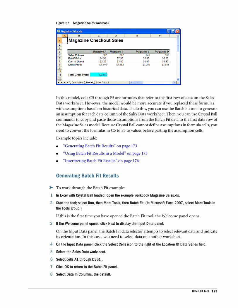
Figure 57 Magazine Sales Workbook
In this model, cells C5 through F5 are formulas that refer to the first row of data on the SalesData worksheet. However, the model would be more accurate if you replaced these formulaswith assumptions based on historical data. To do this, you can use the Batch Fit tool to generatean assumption for each data column of the Sales Data worksheet. Then, you can use Crystal Ballcommands to copy and paste those assumptions from the Batch Fit data to the first data row ofthe Magazine Sales model. Because Crystal Ball cannot define assumptions in formula cells, youneed to convert the formulas in C5 to F5 to values before pasting the assumption cells.
Example topics include:
l “Generating Batch Fit Results” on page 173
l “Using Batch Fit Results in a Model” on page 175
l “Interpreting Batch Fit Results” on page 176
Generating Batch Fit Results
ä To work through the Batch Fit example:
1 In Excel with Crystal Ball loaded, open the example workbook Magazine Sales.xls.
2 Start the tool; select Run, then More Tools, then Batch Fit. (In Microsoft Excel 2007, select More Tools inthe Tools group.)
If this is the first time you have opened the Batch Fit tool, the Welcome panel opens.
3 If the Welcome panel opens, click Next to display the Input Data panel.
On the Input Data panel, the Batch Fit data selector attempts to select relevant data and indicateits orientation. In this case, you need to select data on another worksheet.
4 On the Input Data panel, click the Select Cells icon to the right of the Location Of Data Series field.
5 Select the Sales Data worksheet.
6 Select cells A1 through D361 .
7 Click OK to return to the Batch Fit panel.
8 Select Data In Columns, the default.
Batch Fit Tool 173
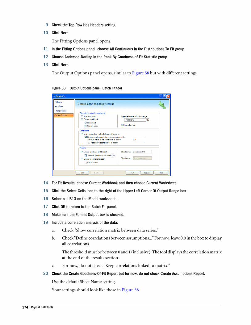
9 Check the Top Row Has Headers setting.
10 Click Next.
The Fitting Options panel opens.
11 In the Fitting Options panel, choose All Continuous in the Distributions To Fit group.
12 Choose Anderson-Darling in the Rank By Goodness-of-Fit Statistic group.
13 Click Next.
The Output Options panel opens, similar to Figure 58 but with different settings.
Figure 58 Output Options panel, Batch Fit tool
14 For Fit Results, choose Current Workbook and then choose Current Worksheet.
15 Click the Select Cells icon to the right of the Upper Left Corner Of Output Range box.
16 Select cell B13 on the Model worksheet.
17 Click OK to return to the Batch Fit panel.
18 Make sure the Format Output box is checked.
19 Include a correlation analysis of the data:
a. Check "Show correlation matrix between data series."
b. Check "Define correlations between assumptions..." For now, leave 0.0 in the box to displayall correlations.
The threshold must be between 0 and 1 (inclusive). The tool displays the correlation matrixat the end of the results section.
c. For now, do not check "Keep correlations linked to matrix."
20 Check the Create Goodness-Of-Fit Report but for now, do not check Create Assumptions Report.
Use the default Sheet Name setting.
Your settings should look like those in Figure 58.
174 Crystal Ball Tools
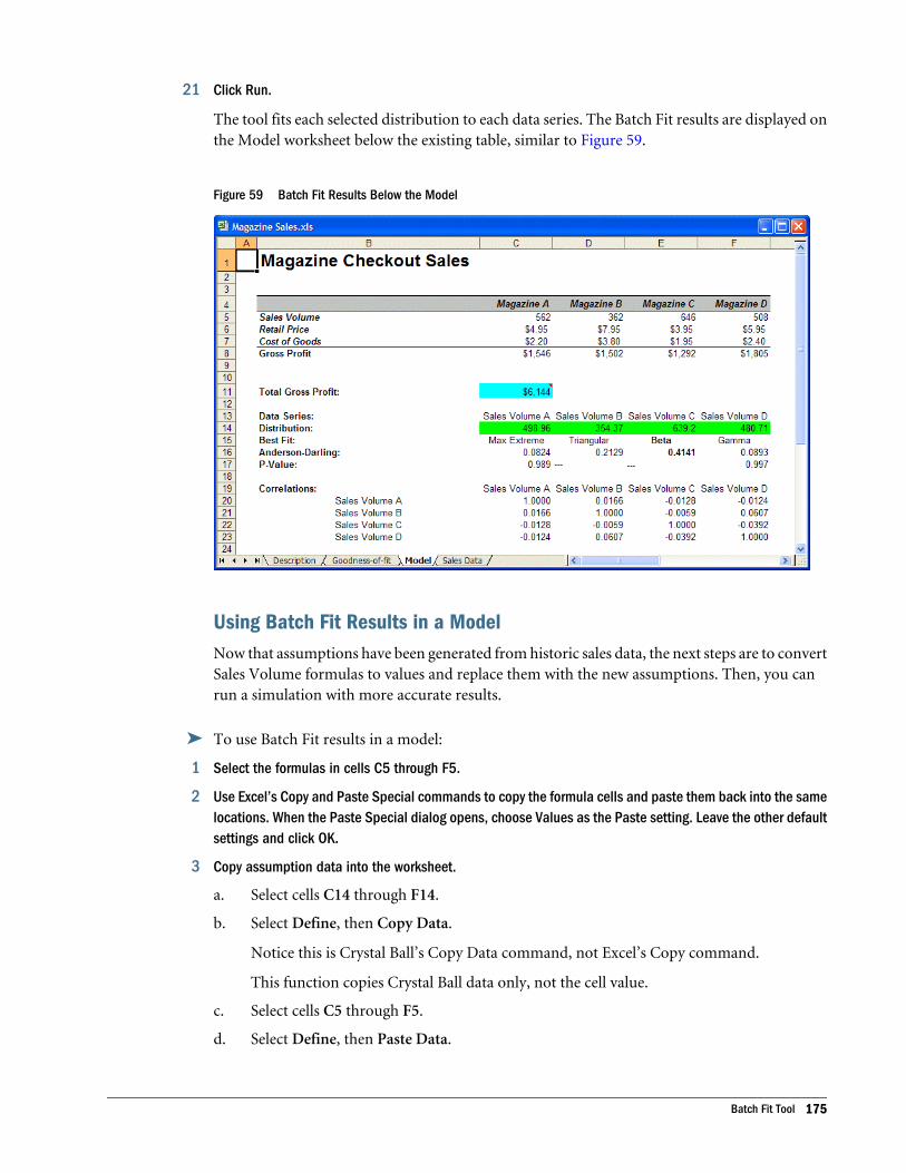
21 Click Run.
The tool fits each selected distribution to each data series. The Batch Fit results are displayed onthe Model worksheet below the existing table, similar to Figure 59.
Figure 59 Batch Fit Results Below the Model
Using Batch Fit Results in a ModelNow that assumptions have been generated from historic sales data, the next steps are to convertSales Volume formulas to values and replace them with the new assumptions. Then, you canrun a simulation with more accurate results.
ä To use Batch Fit results in a model:
1 Select the formulas in cells C5 through F5.
2 Use Excel’s Copy and Paste Special commands to copy the formula cells and paste them back into the samelocations. When the Paste Special dialog opens, choose Values as the Paste setting. Leave the other defaultsettings and click OK.
3 Copy assumption data into the worksheet.
a. Select cells C14 through F14.
b. Select Define, then Copy Data.
Notice this is Crystal Ball’s Copy Data command, not Excel’s Copy command.
This function copies Crystal Ball data only, not the cell value.
c. Select cells C5 through F5.
d. Select Define, then Paste Data.
Batch Fit Tool 175
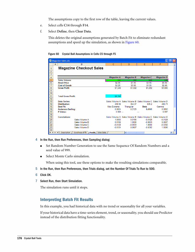
The assumptions copy to the first row of the table, leaving the current values.
e. Select cells C14 through F14.
f. Select Define, then Clear Data.
This deletes the original assumptions generated by Batch Fit to eliminate redundantassumptions and speed up the simulation, as shown in Figure 60.
Figure 60 Crystal Ball Assumptions in Cells C5 through F5
4 In the Run, then Run Preferences, then Sampling dialog:
l Set Random Number Generation to use the Same Sequence Of Random Numbers and aseed value of 999.
l Select Monte Carlo simulation.
When using this tool, use these options to make the resulting simulations comparable.
5 In the Run, then Run Preferences, then Trials dialog, set the Number Of Trials To Run to 500.
6 Click OK.
7 Select Run, then Start Simulation.
The simulation runs until it stops.
Interpreting Batch Fit ResultsIn this example, you had historical data with no trend or seasonality for all your variables.
If your historical data have a time-series element, trend, or seasonality, you should use Predictorinstead of the distribution fitting functionality.
176 Crystal Ball Tools
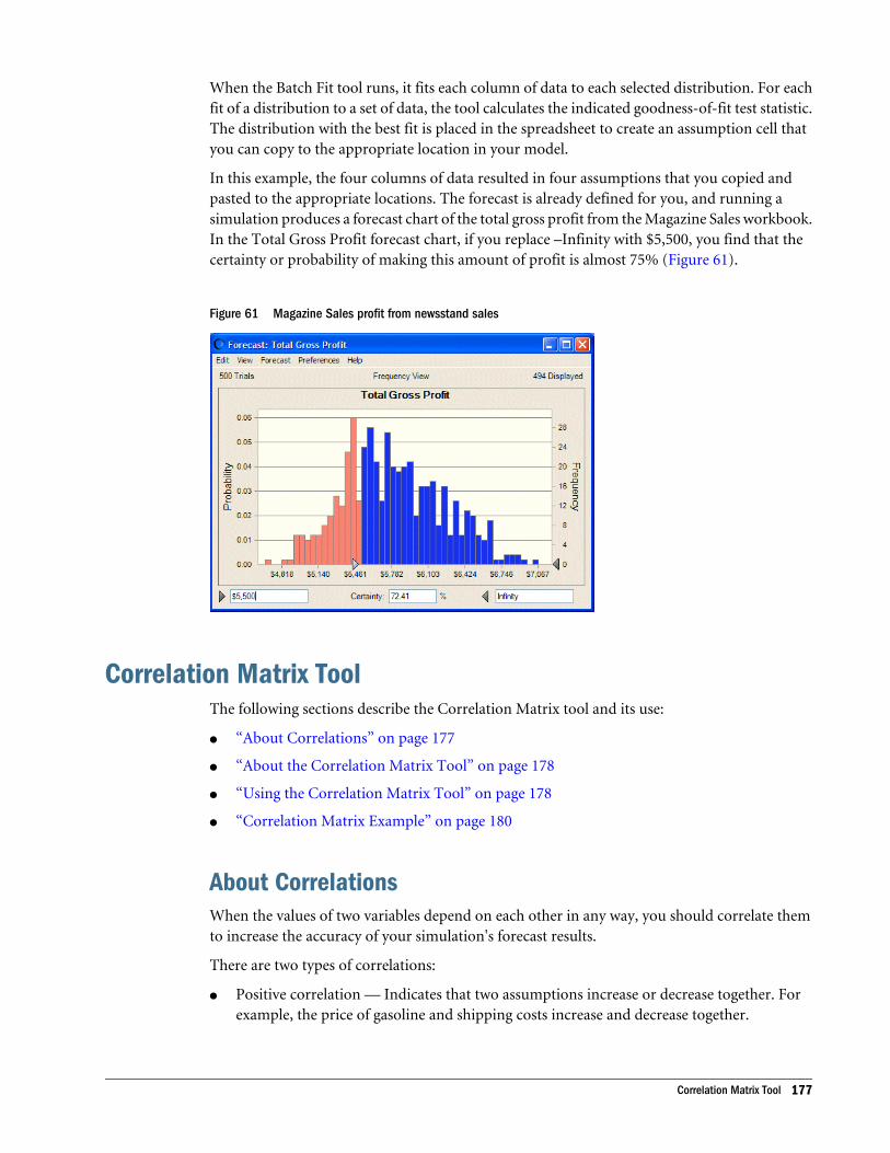
When the Batch Fit tool runs, it fits each column of data to each selected distribution. For eachfit of a distribution to a set of data, the tool calculates the indicated goodness-of-fit test statistic.The distribution with the best fit is placed in the spreadsheet to create an assumption cell thatyou can copy to the appropriate location in your model.
In this example, the four columns of data resulted in four assumptions that you copied andpasted to the appropriate locations. The forecast is already defined for you, and running asimulation produces a forecast chart of the total gross profit from the Magazine Sales workbook.In the Total Gross Profit forecast chart, if you replace –Infinity with $5,500, you find that thecertainty or probability of making this amount of profit is almost 75% (Figure 61).
Figure 61 Magazine Sales profit from newsstand sales
Correlation Matrix ToolThe following sections describe the Correlation Matrix tool and its use:
l “About Correlations” on page 177
l “About the Correlation Matrix Tool” on page 178
l “Using the Correlation Matrix Tool” on page 178
l “Correlation Matrix Example” on page 180
About CorrelationsWhen the values of two variables depend on each other in any way, you should correlate themto increase the accuracy of your simulation's forecast results.
There are two types of correlations:
l Positive correlation — Indicates that two assumptions increase or decrease together. Forexample, the price of gasoline and shipping costs increase and decrease together.
Correlation Matrix Tool 177
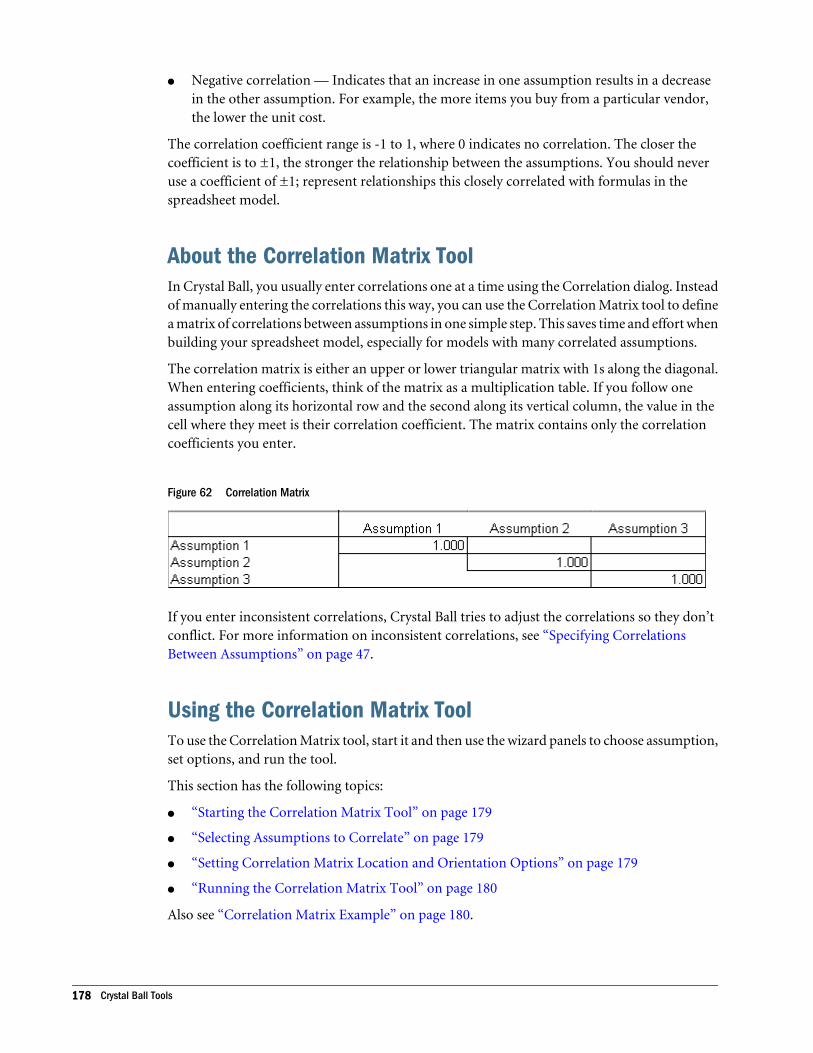
l Negative correlation — Indicates that an increase in one assumption results in a decreasein the other assumption. For example, the more items you buy from a particular vendor,the lower the unit cost.
The correlation coefficient range is -1 to 1, where 0 indicates no correlation. The closer thecoefficient is to ±1, the stronger the relationship between the assumptions. You should neveruse a coefficient of ±1; represent relationships this closely correlated with formulas in thespreadsheet model.
About the Correlation Matrix ToolIn Crystal Ball, you usually enter correlations one at a time using the Correlation dialog. Insteadof manually entering the correlations this way, you can use the Correlation Matrix tool to definea matrix of correlations between assumptions in one simple step. This saves time and effort whenbuilding your spreadsheet model, especially for models with many correlated assumptions.
The correlation matrix is either an upper or lower triangular matrix with 1s along the diagonal.When entering coefficients, think of the matrix as a multiplication table. If you follow oneassumption along its horizontal row and the second along its vertical column, the value in thecell where they meet is their correlation coefficient. The matrix contains only the correlationcoefficients you enter.
Figure 62 Correlation Matrix
If you enter inconsistent correlations, Crystal Ball tries to adjust the correlations so they don’tconflict. For more information on inconsistent correlations, see “Specifying CorrelationsBetween Assumptions” on page 47.
Using the Correlation Matrix ToolTo use the Correlation Matrix tool, start it and then use the wizard panels to choose assumption,set options, and run the tool.
This section has the following topics:
l “Starting the Correlation Matrix Tool” on page 179
l “Selecting Assumptions to Correlate” on page 179
l “Setting Correlation Matrix Location and Orientation Options” on page 179
l “Running the Correlation Matrix Tool” on page 180
Also see “Correlation Matrix Example” on page 180.
178 Crystal Ball Tools
Starting the Correlation Matrix Tool
ä To start the Correlation Matrix tool, select Run, then More Tools, then Correlation Matrix. (InMicrosoft Excel 2007, select More Tools in the Tools group.)
The Select Assumptions panel opens.
Selecting Assumptions to CorrelateThe Select Assumptions panel of the Correlation Matrix tool indicates which assumptions areto be correlated. The settings in this panel include:
l Available Assumptions — Lists all the assumptions defined in the active workbook. To movean assumption into the Selected Assumptions list, either double-click an assumption orselect an assumption and click, then>. You can also make an extended selection using theShift or Ctrl keys.
By default, no assumptions are in this list.
l Top — Moves one or more selected assumptions in the Selected Assumptions list to the topof the list.
l Bottom — Moves one or more selected assumptions in the Selected Assumptions list to thebottom of the list.
l Up — Moves one or more selected assumptions in the Selected Assumptions list up oneposition.
l Down — Moves one or more selected assumptions in the Selected Assumptions list downone position.
l Next — Opens the Specify Options panel for defining correlation matrix options.
Setting Correlation Matrix Location and Orientation OptionsThe Specify Options panel of the Correlation Matrix tool sets two kinds of options, describedin these sections:
l “Location of Matrix Options” on page 179
l “Orientation Options” on page 180
This panel also has the following buttons:
l Back — Returns you to the Select Assumptions panel.
l Start — Creates the correlation matrix according to the options you specify.
Location of Matrix Options
The Location Of Matrix options indicate whether to create the correlation matrix on the activeworksheet or on a new worksheet. Available options include:
l Create A Temporary Correlation Matrix On A New Worksheet — Creates the matrix on anew worksheet. Use this option if you do not want to permanently alter your spreadsheet.
Correlation Matrix Tool 179
After filling in the matrix, click Load The Matrix to enter the coefficients into the model.This is the default matrix location.
l Create And Link To A Correlation Matrix On The Active Worksheet — Creates the matrixon the active worksheet and links it with cell references, so if you change the cells, thecorrelations update automatically. Select this option to embed the correlation matrix in yourmodel. If you select this option, you must indicate where to put the matrix in the modelusing the Specify Upper Left Corner option.
l Specify Upper Left Corner — Enables you to select the origin cell for the top left corner ofthe matrix by either entering the cell reference in the field or clicking on the cell in yourworksheet. This option is only available if you create the matrix on the active worksheet.
l Format Matrix — Adds borders and headings, and changes column widths to make thecorrelation matrix more readable. This option is only available if you create the matrix onthe active worksheet. This option is selected by default.
Orientation Options
The Orientation options indicate whether to make the correlation matrix an upper triangularor a lower triangular matrix.
l Upper Triangular Matrix — Creates the matrix with cells to fill in above the diagonal. Thisis the default.
l Lower Triangular Matrix Creates the matrix with cells to fill in below the diagonal.
Running the Correlation Matrix Tool
ä To run the Correlation Matrix tool when all settings are complete, click Start.
Correlation Matrix ExampleIn the Crystal Ball Examples folder, there is a Portfolio Allocation.xls workbook you can use toexperiment with the Correlation Matrix tool. This spreadsheet calculates the total expectedreturn for an investment model. In this example, you will run a simulation without correlationsand then add the correlations and rerun the simulation for comparison.
ä To start the Correlation Matrix tool:
1 In Excel with Crystal Ball loaded, open the workbook Portfolio Allocation.xls.
2 Set the following options in the Run, then Run Preferences dialog:
l On the Trials tab, set Maximum Number Of Trials to 500.
l On the Sampling tab, set Random Number Generation to Use Same Sequence Of RandomNumbers and set an Initial Seed Value of 999.
l Also on the Sampling tab, set Sampling Method to Monte Carlo.
3 Run a simulation by selecting Run, then Start Simulation.
180 Crystal Ball Tools
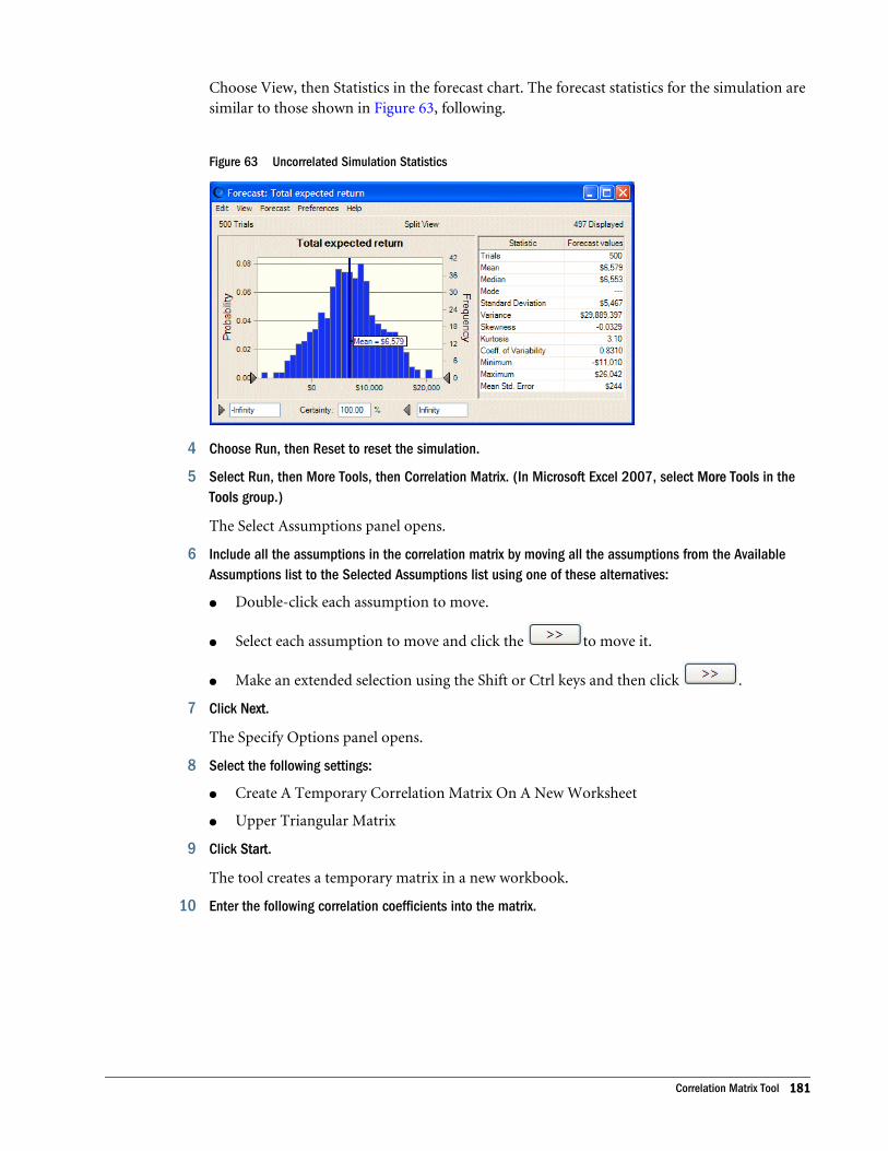
Choose View, then Statistics in the forecast chart. The forecast statistics for the simulation aresimilar to those shown in Figure 63, following.
Figure 63 Uncorrelated Simulation Statistics
4 Choose Run, then Reset to reset the simulation.
5 Select Run, then More Tools, then Correlation Matrix. (In Microsoft Excel 2007, select More Tools in theTools group.)
The Select Assumptions panel opens.
6 Include all the assumptions in the correlation matrix by moving all the assumptions from the AvailableAssumptions list to the Selected Assumptions list using one of these alternatives:
l Double-click each assumption to move.
l Select each assumption to move and click the to move it.
l Make an extended selection using the Shift or Ctrl keys and then click .
7 Click Next.
The Specify Options panel opens.
8 Select the following settings:
l Create A Temporary Correlation Matrix On A New Worksheet
l Upper Triangular Matrix
9 Click Start.
The tool creates a temporary matrix in a new workbook.
10 Enter the following correlation coefficients into the matrix.
Correlation Matrix Tool 181
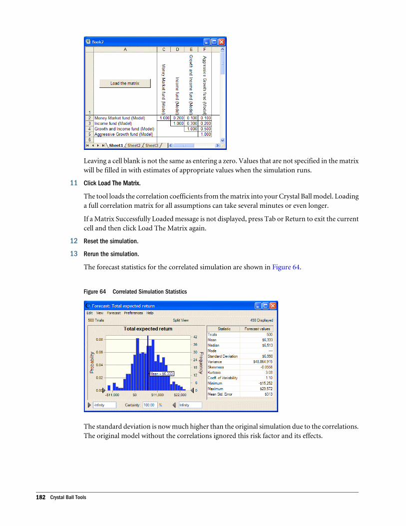
Leaving a cell blank is not the same as entering a zero. Values that are not specified in the matrixwill be filled in with estimates of appropriate values when the simulation runs.
11 Click Load The Matrix.
The tool loads the correlation coefficients from the matrix into your Crystal Ball model. Loadinga full correlation matrix for all assumptions can take several minutes or even longer.
If a Matrix Successfully Loaded message is not displayed, press Tab or Return to exit the currentcell and then click Load The Matrix again.
12 Reset the simulation.
13 Rerun the simulation.
The forecast statistics for the correlated simulation are shown in Figure 64.
Figure 64 Correlated Simulation Statistics
The standard deviation is now much higher than the original simulation due to the correlations.The original model without the correlations ignored this risk factor and its effects.
182 Crystal Ball Tools
Tornado Chart ToolThe Tornado Chart tool measures the impact of each model variable one at a time on a targetforecast. The tool displays the results in two ways, described in these sections:
l “Tornado Chart ” on page 183
l “Spider Chart” on page 185
This method differs from the correlation-based sensitivity method built into Crystal Ball becausethis tool tests each assumption, decision variable, precedent, or cell independently. Whileanalyzing one variable, the tool freezes the other variables at their base values. This measures theeffect of each variable on the forecast cell while removing the effects of the other variables. Thismethod is also known as "one-at-a-time perturbation" or "parametric analysis."
The Tornado Chart tool is useful for:
l Measuring the sensitivity of variables that you have defined in Crystal Ball.
l Quickly pre-screening the variables in your model to determine which ones are goodcandidates to define as assumptions or decision variables. You can do this by testing theprecedent variables of any formula cell. See for more information on precedents.
The following sections describe how to create and use tornado charts and spider charts:
l “Using the Tornado Chart Tool” on page 185
l “Tornado Chart Example” on page 188
l “Limitations of the Tornado Chart Tool” on page 191
Tornado Chart The Tornado Chart tool tests the range of each variable at percentiles you specify and thencalculates the value of the forecast at each point. The tornado chart (Figure 65)illustrates theswing between the maximum and minimum forecast values for each variable. The variable thatcauses the largest swing is displayed at the top and the variable that causes the smallest swing isdisplayed at the bottom. The upper variables have the most effect on the forecast, and the lowervariables have the least effect on the forecast.
Tornado Chart Tool 183

Figure 65 Tornado Chart
The bars next to each variable represent the forecast value range across the variable tested, asdiscussed above. Next to the bars are the values of the variables that produced the greatest swingin the forecast values. The bar colors indicate the direction of the relationship between thevariables and the forecast.
For variables that have a positive effect on the forecast, the upside of the variable (shown in blue)is to the right of the base case (the initial value in the cell before running the simulation) andthe downside of the variable (shown in red) is to the left side of the base case. For variables thathave a reverse relationship with the forecast, the bars are reversed.
When a variable’s relationship with the forecast is not strictly increasing or decreasing, it is callednon-monotonic. In other words, if the minimum or maximum values of the forecast range donot occur at the extreme endpoints of the testing range for the variable, the variable has a non-monotonic relationship with the forecast (Figure 66).
Figure 66 A non-monotonic variable
If one or more variables are non-monotonic, all the variable bars are the same color all the wayacross.
184 Crystal Ball Tools
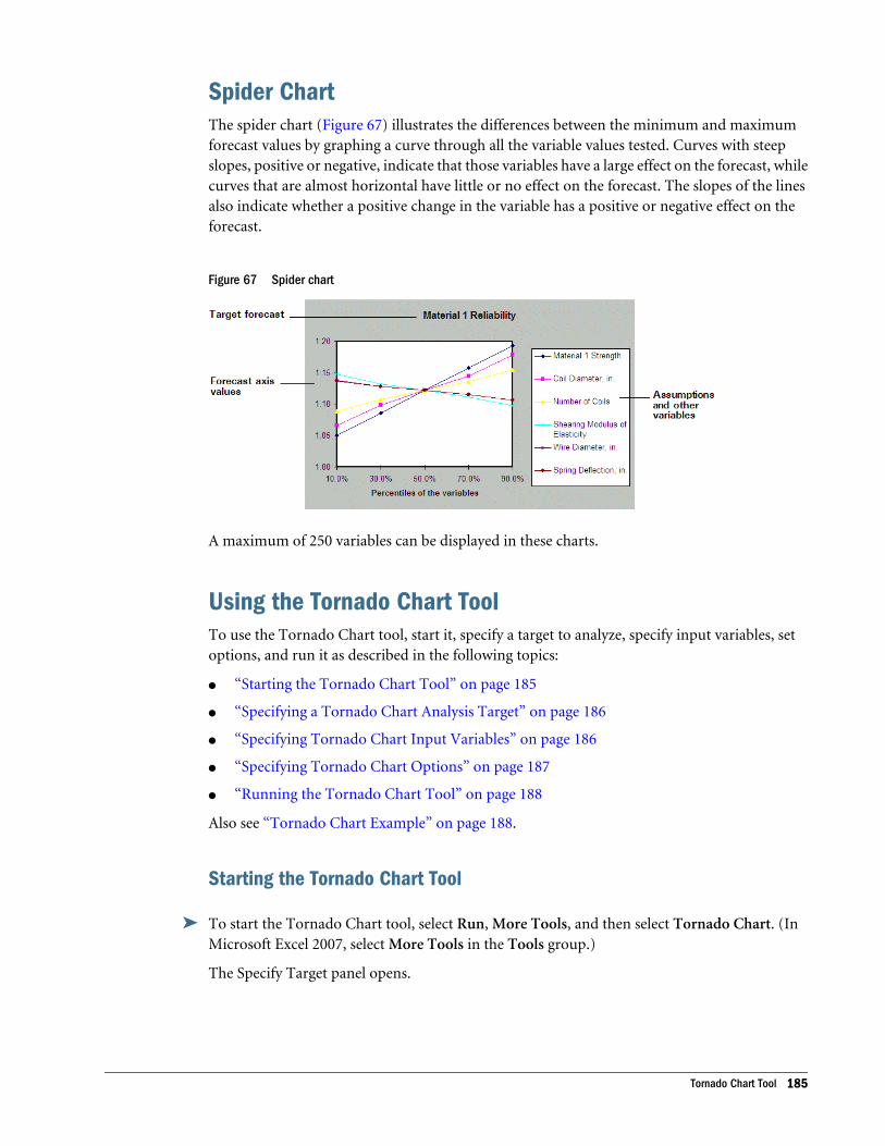
Spider ChartThe spider chart (Figure 67) illustrates the differences between the minimum and maximumforecast values by graphing a curve through all the variable values tested. Curves with steepslopes, positive or negative, indicate that those variables have a large effect on the forecast, whilecurves that are almost horizontal have little or no effect on the forecast. The slopes of the linesalso indicate whether a positive change in the variable has a positive or negative effect on theforecast.
Figure 67 Spider chart
A maximum of 250 variables can be displayed in these charts.
Using the Tornado Chart ToolTo use the Tornado Chart tool, start it, specify a target to analyze, specify input variables, setoptions, and run it as described in the following topics:
l “Starting the Tornado Chart Tool” on page 185
l “Specifying a Tornado Chart Analysis Target” on page 186
l “Specifying Tornado Chart Input Variables” on page 186
l “Specifying Tornado Chart Options” on page 187
l “Running the Tornado Chart Tool” on page 188
Also see “Tornado Chart Example” on page 188.
Starting the Tornado Chart Tool
ä To start the Tornado Chart tool, select Run, More Tools, and then select Tornado Chart. (InMicrosoft Excel 2007, select More Tools in the Tools group.)
The Specify Target panel opens.
Tornado Chart Tool 185
Specifying a Tornado Chart Analysis TargetThe Specify Target panel in the Tornado Chart tool indicates which forecast or formula cell toanalyze. The Specify Target panel contains the following settings:
l Forecast List — Lists all the forecast cells in all open spreadsheets. When you select a forecastfrom the list, its cell information is automatically displayed in the Enter Target Cell field.The first forecast is selected by default.
l Enter Target Cell — Describes the cell location of the selected forecast or formula. If youselect a forecast from the list above, the cell information is automatically displayed in thisfield. You can use this field to select a formula cell instead of a forecast.
l Next — Opens the Specify Input Variables panel.
When settings are complete, click Next to open the Specify Input Variables panel.
Specifying Tornado Chart Input VariablesThe Specify Input Variables panel of the Tornado Chart tool specifies the assumptions, decisionvariables, and precedents to include in the tornado and spider charts. You can include any valuecell in your tornado chart calculations. However, the cells are usually:
l Assumptions — Cells defined as assumptions in Crystal Ball.
l Decision variables — Cells defined as decision variables in Crystal Ball.
l Precedents — All cells within the active spreadsheet that are referenced as part of the formulaor a sub-formula of the target cell. Precedents for this tool are handled differently thanstandard Excel precedents in that they cannot trace beyond the active spreadsheet. Therefore,you can only use precedents on the active spreadsheet as input variables.
The Specify Input Variables panel includes these settings:
l Input Variable List — Lists all the variables selected for the tornado and spider charts.
l Add Assumptions — Adds all assumptions from all open worksheets to the input variablelist.
l Add Decision Variables — Adds all decision variables from all open worksheets to the inputvariable list.
l Add Precedents — Adds all precedents of the target cell from all open worksheets to theinput variable list.
l Add Range — Lets you select a range of cells from the open worksheet to add to the inputvariable list. If you click this button, an Input panel opens, asking you to enter a cell rangeor to select a range of cells from the spreadsheet. You must click OK to accept the selectedrange.
l Remove — This button removes the selected variable from the input variable list.
l Remove All — Removes all of the items from the input variable list.
l Back — Returns to the Specify Target panel.
l Next — Opens the Specify Options panel.
186 Crystal Ball Tools
When settings are complete, click Next to open the Specify Options panel.
Specifying Tornado Chart OptionsThe Specify Options panel of the Tornado Chart tool sets options that control the tool. Thegroups of options in this panel are described in the following sections:
l “Tornado Method Options” on page 187
l “Tornado Input Options” on page 187
l “Tornado Output Options” on page 187
Other controls are:
l Back — Returns to the Specify Input Variables panel.
l Start — Starts the tool, generating the tornado and spider charts.
Tornado Method Options
The Tornado Method options in this panel are:
l Percentiles Of The Variables — Indicates that the tool should test the variables usingpercentiles of the assumption distributions or percentiles of the decision variable ranges.This is the default.
l Percentage Deviations From The Base Case — Indicates that the tool should test the variablesusing small changes that are specified percentages away from the base case. This is the onlyoption available if you selected variables other than assumptions or decision variables. Thetool treats discrete decision variables as continuous for this second method.
Tornado Input Options
The Tornado Input options include:
l Testing Range — Defines the range in which the tool samples the variables. The choices areeither: the percentile range (if the tornado method is Percentiles Of The Variables) or thepercent from the base case (if the tornado method is Percentage Deviations From The BaseCase). The default is 10% to 90% percentiles or -10% to 10% deviation.
l Testing Points — Defines how many values to test in the testing range. The testing pointsare evenly distributed across the testing range. Testing more points than just end pointsdetects non-monotonic variable relationships. The default is five testing points.
l For Base Case Specifies whether to define the base case as either the existing cell values orthe median values of the variables. If the tornado is based on a percentage deviation, onlythe cell values option is available. The default is the median cell values.
Tornado Output Options
The Tornado Output options are:
Tornado Chart Tool 187
l Tornado Chart — Generates a tornado chart showing the sensitivity of the variables usingrange bars.
l Spider Chart — Generates a spider chart showing the sensitivity of the variables using slopingcurves.
l Show Top Variables — Indicates how many variables to include in the tornado charts ifthere are a lot of variables. The charts can only clearly show about 20 variables.
Running the Tornado Chart Tool
ä When all settings are complete, click Start to run the Tornado Chart tool and generate selectedcharts.
Tornado Chart ExampleIn the Crystal Ball Examples folder, there is a Reliability.xls workbook you can use to experimentwith the Tornado Chart tool. This spreadsheet model predicts the reliability of a spring usingthree different construction materials. This section includes the following example topics:
l “Generating Tornado and Spider Charts” on page 188
l “Interpreting Tornado and Spider Chart Results” on page 190
Generating Tornado and Spider Charts
ä To run the Tornado Chart tool:
1 In Excel with Crystal Ball loaded, open the workbook Reliability.xls.
If you have any other spreadsheets open, close them first, because the tool gathers all CrystalBall definitions from all open workbooks.
2 Select Run, then More Tools, then Tornado Chart. (In Microsoft Excel 2007, select More Tools in the Toolsgroup.)
The Specify Target panel opens. All of the forecasts from Reliability.xls are displayed in the list.
3 Select the "Material 1 Reliability" forecast.
4 Click Next.
The Specify Input Variables panel opens.
You can include any value cell in your tornado chart calculations, using cell names if available.However, the cells are usually defined as one of the following types:
l Assumptions — Cells defined as assumptions in Crystal Ball. For more information aboutassumptions, see “About Assumptions and Probability Distributions” on page 38.
l Decision variables — Cells defined as decision variables in Crystal Ball. For moreinformation about defining decision variables, see “Defining Decision Variable Cells” onpage 63.
188 Crystal Ball Tools
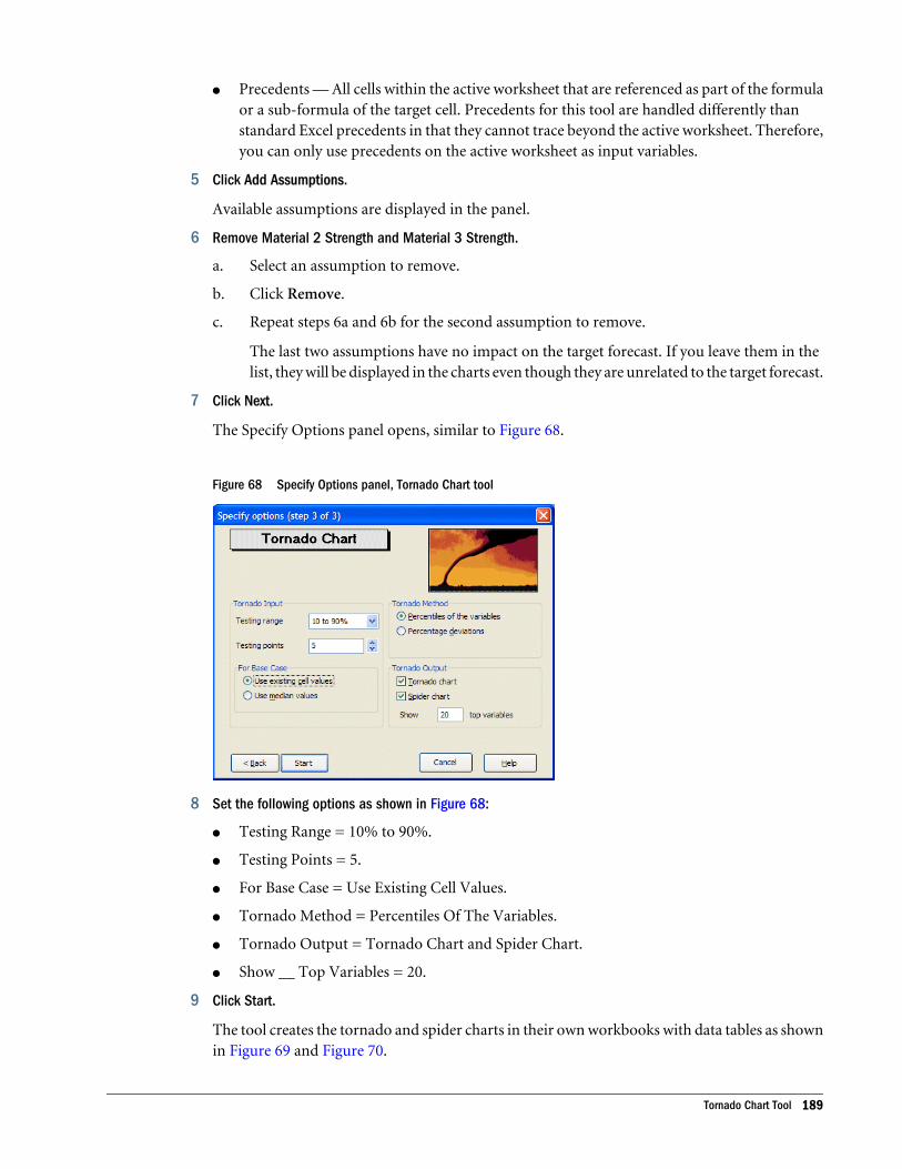
l Precedents — All cells within the active worksheet that are referenced as part of the formulaor a sub-formula of the target cell. Precedents for this tool are handled differently thanstandard Excel precedents in that they cannot trace beyond the active worksheet. Therefore,you can only use precedents on the active worksheet as input variables.
5 Click Add Assumptions.
Available assumptions are displayed in the panel.
6 Remove Material 2 Strength and Material 3 Strength.
a. Select an assumption to remove.
b. Click Remove.
c. Repeat steps 6a and 6b for the second assumption to remove.
The last two assumptions have no impact on the target forecast. If you leave them in thelist, they will be displayed in the charts even though they are unrelated to the target forecast.
7 Click Next.
The Specify Options panel opens, similar to Figure 68.
Figure 68 Specify Options panel, Tornado Chart tool
8 Set the following options as shown in Figure 68:
l Testing Range = 10% to 90%.
l Testing Points = 5.
l For Base Case = Use Existing Cell Values.
l Tornado Method = Percentiles Of The Variables.
l Tornado Output = Tornado Chart and Spider Chart.
l Show __ Top Variables = 20.
9 Click Start.
The tool creates the tornado and spider charts in their own workbooks with data tables as shownin Figure 69 and Figure 70.
Tornado Chart Tool 189
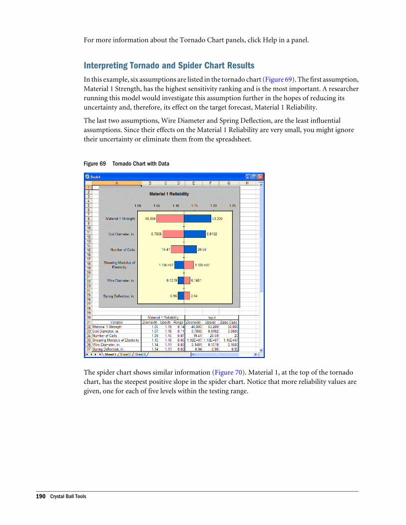
For more information about the Tornado Chart panels, click Help in a panel.
Interpreting Tornado and Spider Chart ResultsIn this example, six assumptions are listed in the tornado chart (Figure 69). The first assumption,Material 1 Strength, has the highest sensitivity ranking and is the most important. A researcherrunning this model would investigate this assumption further in the hopes of reducing itsuncertainty and, therefore, its effect on the target forecast, Material 1 Reliability.
The last two assumptions, Wire Diameter and Spring Deflection, are the least influentialassumptions. Since their effects on the Material 1 Reliability are very small, you might ignoretheir uncertainty or eliminate them from the spreadsheet.
Figure 69 Tornado Chart with Data
The spider chart shows similar information (Figure 70). Material 1, at the top of the tornadochart, has the steepest positive slope in the spider chart. Notice that more reliability values aregiven, one for each of five levels within the testing range.
190 Crystal Ball Tools
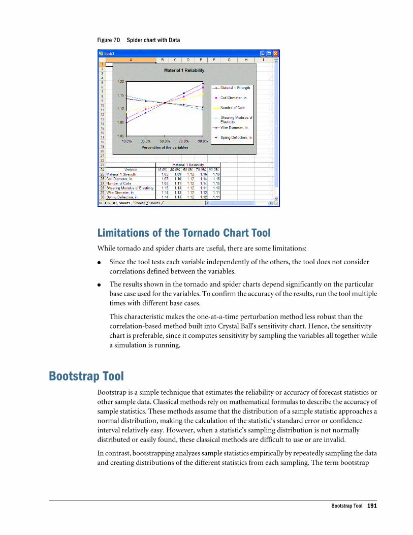
Figure 70 Spider chart with Data
Limitations of the Tornado Chart ToolWhile tornado and spider charts are useful, there are some limitations:
l Since the tool tests each variable independently of the others, the tool does not considercorrelations defined between the variables.
l The results shown in the tornado and spider charts depend significantly on the particularbase case used for the variables. To confirm the accuracy of the results, run the tool multipletimes with different base cases.
This characteristic makes the one-at-a-time perturbation method less robust than thecorrelation-based method built into Crystal Ball's sensitivity chart. Hence, the sensitivitychart is preferable, since it computes sensitivity by sampling the variables all together whilea simulation is running.
Bootstrap ToolBootstrap is a simple technique that estimates the reliability or accuracy of forecast statistics orother sample data. Classical methods rely on mathematical formulas to describe the accuracy ofsample statistics. These methods assume that the distribution of a sample statistic approaches anormal distribution, making the calculation of the statistic’s standard error or confidenceinterval relatively easy. However, when a statistic’s sampling distribution is not normallydistributed or easily found, these classical methods are difficult to use or are invalid.
In contrast, bootstrapping analyzes sample statistics empirically by repeatedly sampling the dataand creating distributions of the different statistics from each sampling. The term bootstrap
Bootstrap Tool 191
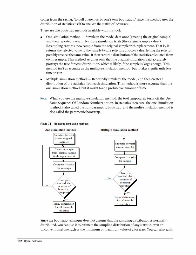
comes from the saying, "to pull oneself up by one’s own bootstraps," since this method uses thedistribution of statistics itself to analyze the statistics’ accuracy.
There are two bootstrap methods available with this tool:
l One-simulation method — Simulates the model data once (creating the original sample)and then repeatedly resamples those simulation trials (the original sample values).Resampling creates a new sample from the original sample with replacement. That is, itreturns the selected value to the sample before selecting another value, letting the selectorpossibly reselect the same value. It then creates a distribution of the statistics calculated fromeach resample. This method assumes only that the original simulation data accuratelyportrays the true forecast distribution, which is likely if the sample is large enough. Thismethod isn’t as accurate as the multiple-simulation method, but it takes significantly lesstime to run.
l Multiple-simulation method — Repeatedly simulates the model, and then creates adistribution of the statistics from each simulation. This method is more accurate than theone-simulation method, but it might take a prohibitive amount of time.
Note: When you use the multiple-simulation method, the tool temporarily turns off the UseSame Sequence Of Random Numbers option. In statistics literature, the one-simulationmethod is also called the non-parametric bootstrap, and the multi-simulation method isalso called the parametric bootstrap.
Figure 71 Bootstrap simulation methods
Since the bootstrap technique does not assume that the sampling distribution is normallydistributed, you can use it to estimate the sampling distribution of any statistic, even anunconventional one such as the minimum or maximum value of a forecast. You can also easily
192 Crystal Ball Tools
estimate complex statistics, such as the correlation coefficient of two data sets, or combinationsof statistics, such as the ratio of a mean to a variance.
To estimate the accuracy of Latin Hypercube statistics, you must use the multiple-simulationmethod.
The following sections describe how to use the Bootstrap tool:
l “Using the Bootstrap Tool” on page 193
l “Bootstrap Example” on page 195
Using the Bootstrap ToolTo use the Bootstrap tool, you start it, define a target forecast or formula cell, choose a bootstrapmethod, set options, and then run the tool. The following sections describe these steps:
l “Starting the Bootstrap Tool” on page 193
l “Using the Bootstrap Welcome Panel” on page 193
l “Specifying Forecasts to Analyze with the Bootstrap Tool” on page 194
l “Specifying a Bootstrap Tool Method” on page 194
l “Setting Bootstrap Options” on page 195
l “Running the Bootstrap Tool” on page 195
Also see “Bootstrap Example” on page 195.
Starting the Bootstrap Tool
ä To start the Bootstrap tool, select Run, then More Tools, and then Bootstrap. (In MicrosoftExcel 2007, select More Tools in the Tools group.)
The first time you start Bootstrap, the Welcome panel opens; otherwise, the Target Forecastpanel opens.
Using the Bootstrap Welcome PanelThe Welcome panel opens the first time you use the Bootstrap tool. It describes the tool and itsuse. The controls for this panel are:
l Next — Opens the Target Forecast panel for choosing a target forecast.
l Run — Runs the Bootstrap tool and generates results.
Bootstrap Tool 193
ä Click Next to continue to the Target Forecast panel.
Specifying Forecasts to Analyze with the Bootstrap ToolThe Target Forecast panel of the Bootstrap tool indicates which forecast, formula cell or cellrange to analyze. The controls for this panel are:
l Forecast list — Lists all the forecast cells in all open spreadsheets. When you select a forecastfrom the list, its cell information is automatically displayed in the data range field. The firstforecast is selected by default.
l Data range — Describes the cell location of the selected forecast or formula. If you select aforecast from the forecast list, the cell information is automatically displayed in this field.You can use this field to select a formula cell instead of a forecast. If you choose a data range,the data must be a single contiguous (connected) block.
l Back — Opens the Welcome panel.
l Next — Opens the Method panel for defining which simulation method to use.
l Run — Runs the Bootstrap tool and generates results.
ä Select a target forecast and then click Next to select a simulation method.
Specifying a Bootstrap Tool MethodThe Method panel of the Bootstrap tool specifies a bootstrap method and analysis type. It hasthe following controls:
l Bootstrap Method — Selects whether to use the one-simulation or multiple-simulationbootstrap method. For more information on these two methods, see “Bootstrap Tool” onpage 191. The default is the one-simulation method.
l Analyze Distributions Of — Selects whether to analyze distributions of statistics, percentiles,or capability metrics. If you select Percentiles, you must complete the Percentiles options.The default is Statistics.
l Percentiles — If Percentiles is selected in Analyze Distributions Of, selects which targetpercentiles to analyze. You can select either: deciles (the 10, 20, 30, 40, 50, 60, 70, 80, and 90percentiles); 2, 5, 50, 90, and 97.5 percentiles; or a custom list of percentiles you enter in thefield (between 0 and 100, exclusive) separated by commas.
l Back — Returns to the Target Forecast panel for specifying a target forecast.
l Next — Opens the Options panel for defining sample and display options.
l Run — Runs the Bootstrap tool and generates results.
194 Crystal Ball Tools
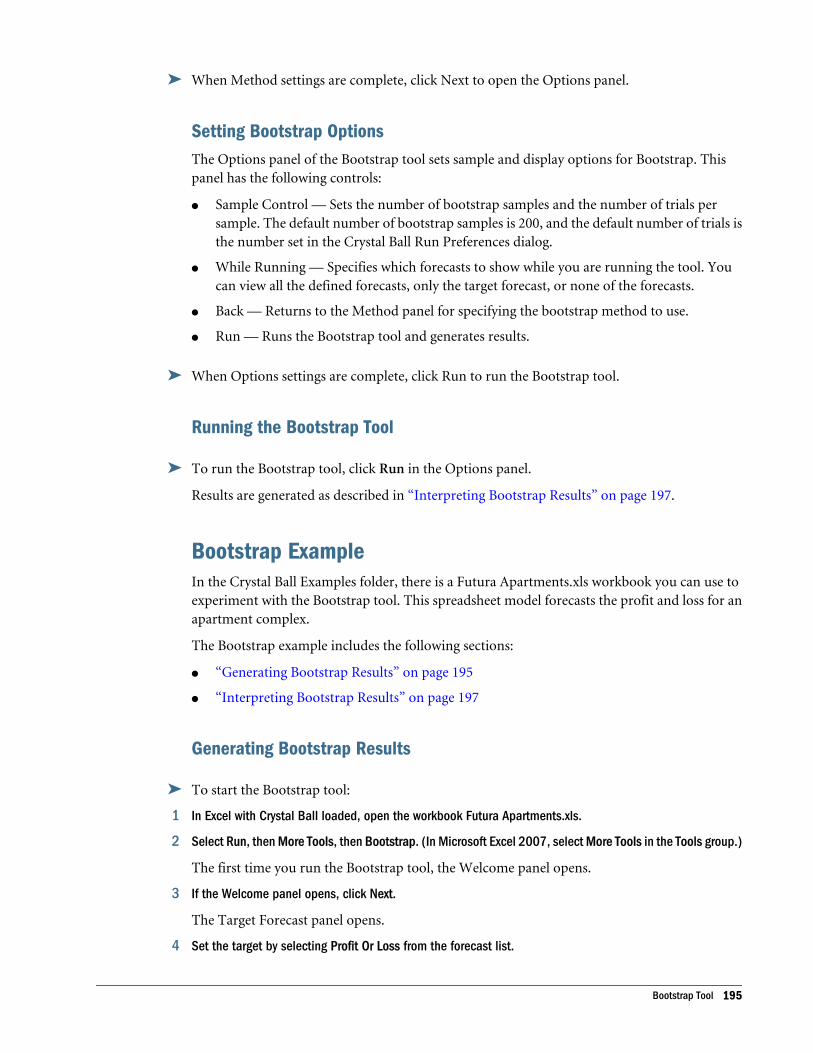
ä When Method settings are complete, click Next to open the Options panel.
Setting Bootstrap OptionsThe Options panel of the Bootstrap tool sets sample and display options for Bootstrap. Thispanel has the following controls:
l Sample Control — Sets the number of bootstrap samples and the number of trials persample. The default number of bootstrap samples is 200, and the default number of trials isthe number set in the Crystal Ball Run Preferences dialog.
l While Running — Specifies which forecasts to show while you are running the tool. Youcan view all the defined forecasts, only the target forecast, or none of the forecasts.
l Back — Returns to the Method panel for specifying the bootstrap method to use.
l Run — Runs the Bootstrap tool and generates results.
ä When Options settings are complete, click Run to run the Bootstrap tool.
Running the Bootstrap Tool
ä To run the Bootstrap tool, click Run in the Options panel.
Results are generated as described in “Interpreting Bootstrap Results” on page 197.
Bootstrap ExampleIn the Crystal Ball Examples folder, there is a Futura Apartments.xls workbook you can use toexperiment with the Bootstrap tool. This spreadsheet model forecasts the profit and loss for anapartment complex.
The Bootstrap example includes the following sections:
l “Generating Bootstrap Results” on page 195
l “Interpreting Bootstrap Results” on page 197
Generating Bootstrap Results
ä To start the Bootstrap tool:
1 In Excel with Crystal Ball loaded, open the workbook Futura Apartments.xls.
2 Select Run, then More Tools, then Bootstrap. (In Microsoft Excel 2007, select More Tools in the Tools group.)
The first time you run the Bootstrap tool, the Welcome panel opens.
3 If the Welcome panel opens, click Next.
The Target Forecast panel opens.
4 Set the target by selecting Profit Or Loss from the forecast list.
Bootstrap Tool 195
Instead, you could choose "Or, enter a data range:" and enter a range of spreadsheet data cellsto be used for resampling.
5 Click Next.
The Method panel opens.
6 Make sure the one-simulation method and the statistics options are selected.
If you choose Percentiles and then choose Custom, you can select 0 or 100 as well as valuesbetween these.
7 Click Next.
The Options panel opens.
8 Set the following options:
l Number Of Bootstrap Samples = 200
l Number Of Trials Per Sample = 500
l Show Only Target Forecast is selected
9 Click Run.
The Bootstrap tool displays a forecast chart of the distributions for each statistic and creates aworkbook summarizing the data (Figure 72).
Note: If distribution fitting is turned on for the target forecast, it is turned off during the runningof simulations within the tool. When simulations finish, distribution fitting is restored.
196 Crystal Ball Tools
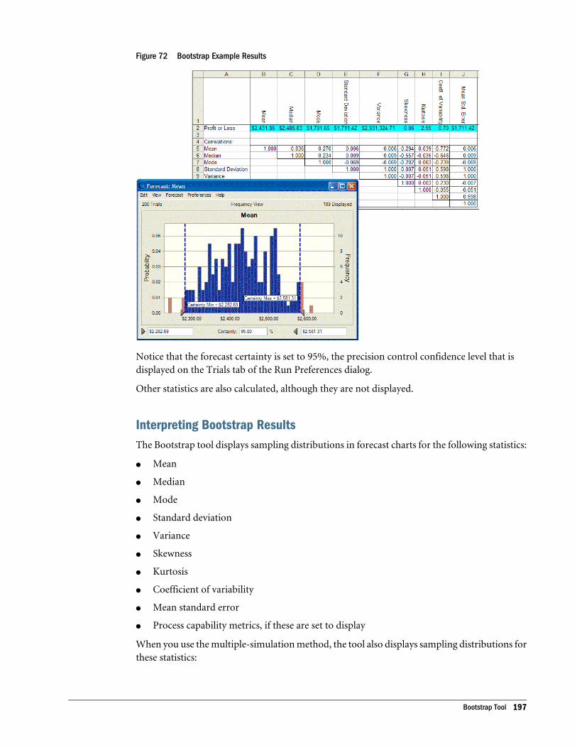
Figure 72 Bootstrap Example Results
Notice that the forecast certainty is set to 95%, the precision control confidence level that isdisplayed on the Trials tab of the Run Preferences dialog.
Other statistics are also calculated, although they are not displayed.
Interpreting Bootstrap ResultsThe Bootstrap tool displays sampling distributions in forecast charts for the following statistics:
l Mean
l Median
l Mode
l Standard deviation
l Variance
l Skewness
l Kurtosis
l Coefficient of variability
l Mean standard error
l Process capability metrics, if these are set to display
When you use the multiple-simulation method, the tool also displays sampling distributions forthese statistics:
Bootstrap Tool 197
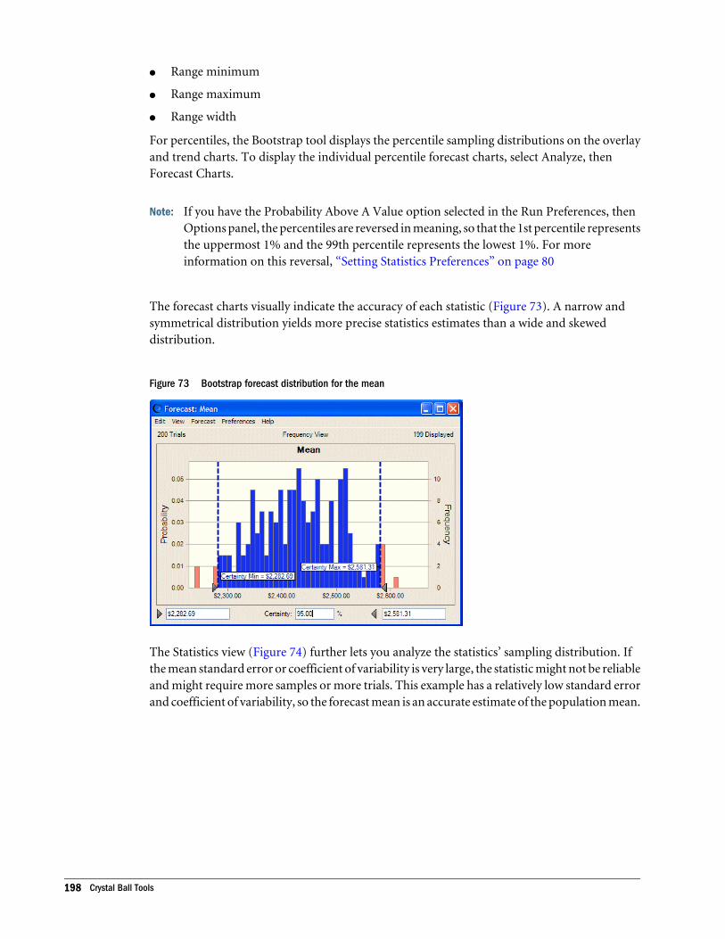
l Range minimum
l Range maximum
l Range width
For percentiles, the Bootstrap tool displays the percentile sampling distributions on the overlayand trend charts. To display the individual percentile forecast charts, select Analyze, thenForecast Charts.
Note: If you have the Probability Above A Value option selected in the Run Preferences, thenOptions panel, the percentiles are reversed in meaning, so that the 1st percentile representsthe uppermost 1% and the 99th percentile represents the lowest 1%. For moreinformation on this reversal, “Setting Statistics Preferences” on page 80
The forecast charts visually indicate the accuracy of each statistic (Figure 73). A narrow andsymmetrical distribution yields more precise statistics estimates than a wide and skeweddistribution.
Figure 73 Bootstrap forecast distribution for the mean
The Statistics view (Figure 74) further lets you analyze the statistics’ sampling distribution. Ifthe mean standard error or coefficient of variability is very large, the statistic might not be reliableand might require more samples or more trials. This example has a relatively low standard errorand coefficient of variability, so the forecast mean is an accurate estimate of the population mean.
198 Crystal Ball Tools
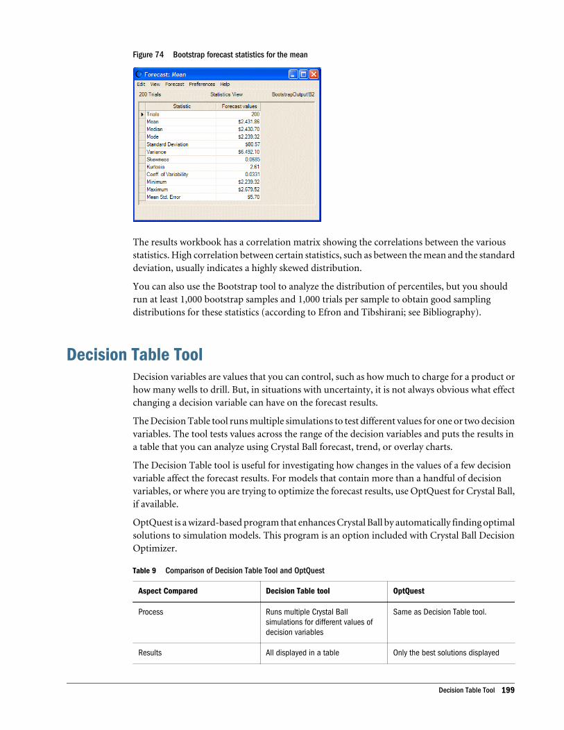
Figure 74 Bootstrap forecast statistics for the mean
The results workbook has a correlation matrix showing the correlations between the variousstatistics. High correlation between certain statistics, such as between the mean and the standarddeviation, usually indicates a highly skewed distribution.
You can also use the Bootstrap tool to analyze the distribution of percentiles, but you shouldrun at least 1,000 bootstrap samples and 1,000 trials per sample to obtain good samplingdistributions for these statistics (according to Efron and Tibshirani; see Bibliography).
Decision Table ToolDecision variables are values that you can control, such as how much to charge for a product orhow many wells to drill. But, in situations with uncertainty, it is not always obvious what effectchanging a decision variable can have on the forecast results.
The Decision Table tool runs multiple simulations to test different values for one or two decisionvariables. The tool tests values across the range of the decision variables and puts the results ina table that you can analyze using Crystal Ball forecast, trend, or overlay charts.
The Decision Table tool is useful for investigating how changes in the values of a few decisionvariable affect the forecast results. For models that contain more than a handful of decisionvariables, or where you are trying to optimize the forecast results, use OptQuest for Crystal Ball,if available.
OptQuest is a wizard-based program that enhances Crystal Ball by automatically finding optimalsolutions to simulation models. This program is an option included with Crystal Ball DecisionOptimizer.
Table 9 Comparison of Decision Table Tool and OptQuest
Aspect Compared Decision Table tool OptQuest
Process Runs multiple Crystal Ballsimulations for different values ofdecision variables
Same as Decision Table tool.
Results All displayed in a table Only the best solutions displayed
Decision Table Tool 199
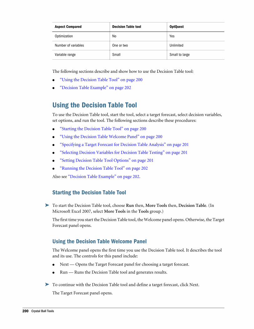
Aspect Compared Decision Table tool OptQuest
Optimization No Yes
Number of variables One or two Unlimited
Variable range Small Small to large
The following sections describe and show how to use the Decision Table tool:
l “Using the Decision Table Tool” on page 200
l “Decision Table Example” on page 202
Using the Decision Table ToolTo use the Decision Table tool, start the tool, select a target forecast, select decision variables,set options, and run the tool. The following sections describe these procedures:
l “Starting the Decision Table Tool” on page 200
l “Using the Decision Table Welcome Panel” on page 200
l “Specifying a Target Forecast for Decision Table Analysis” on page 201
l “Selecting Decision Variables for Decision Table Testing” on page 201
l “Setting Decision Table Tool Options” on page 201
l “Running the Decision Table Tool” on page 202
Also see “Decision Table Example” on page 202.
Starting the Decision Table Tool
ä To start the Decision Table tool, choose Run then, More Tools then, Decision Table. (InMicrosoft Excel 2007, select More Tools in the Tools group.)
The first time you start the Decision Table tool, the Welcome panel opens. Otherwise, the TargetForecast panel opens.
Using the Decision Table Welcome PanelThe Welcome panel opens the first time you use the Decision Table tool. It describes the tooland its use. The controls for this panel include:
l Next — Opens the Target Forecast panel for choosing a target forecast.
l Run — Runs the Decision Table tool and generates results.
ä To continue with the Decision Table tool and define a target forecast, click Next.
The Target Forecast panel opens.
200 Crystal Ball Tools
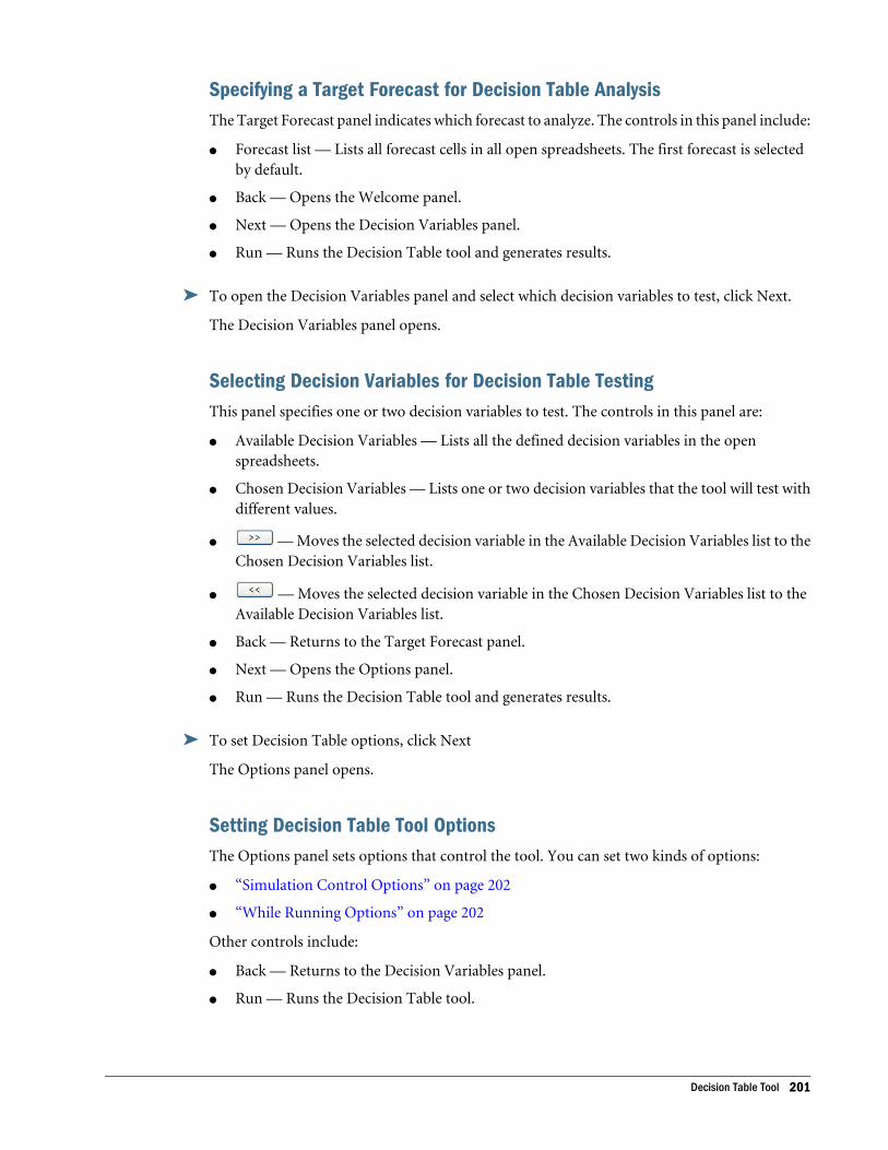
Specifying a Target Forecast for Decision Table AnalysisThe Target Forecast panel indicates which forecast to analyze. The controls in this panel include:
l Forecast list — Lists all forecast cells in all open spreadsheets. The first forecast is selectedby default.
l Back — Opens the Welcome panel.
l Next — Opens the Decision Variables panel.
l Run — Runs the Decision Table tool and generates results.
ä To open the Decision Variables panel and select which decision variables to test, click Next.
The Decision Variables panel opens.
Selecting Decision Variables for Decision Table TestingThis panel specifies one or two decision variables to test. The controls in this panel are:
l Available Decision Variables — Lists all the defined decision variables in the openspreadsheets.
l Chosen Decision Variables — Lists one or two decision variables that the tool will test withdifferent values.
l — Moves the selected decision variable in the Available Decision Variables list to theChosen Decision Variables list.
l — Moves the selected decision variable in the Chosen Decision Variables list to theAvailable Decision Variables list.
l Back — Returns to the Target Forecast panel.
l Next — Opens the Options panel.
l Run — Runs the Decision Table tool and generates results.
ä To set Decision Table options, click Next
The Options panel opens.
Setting Decision Table Tool OptionsThe Options panel sets options that control the tool. You can set two kinds of options:
l “Simulation Control Options” on page 202
l “While Running Options” on page 202
Other controls include:
l Back — Returns to the Decision Variables panel.
l Run — Runs the Decision Table tool.
Decision Table Tool 201
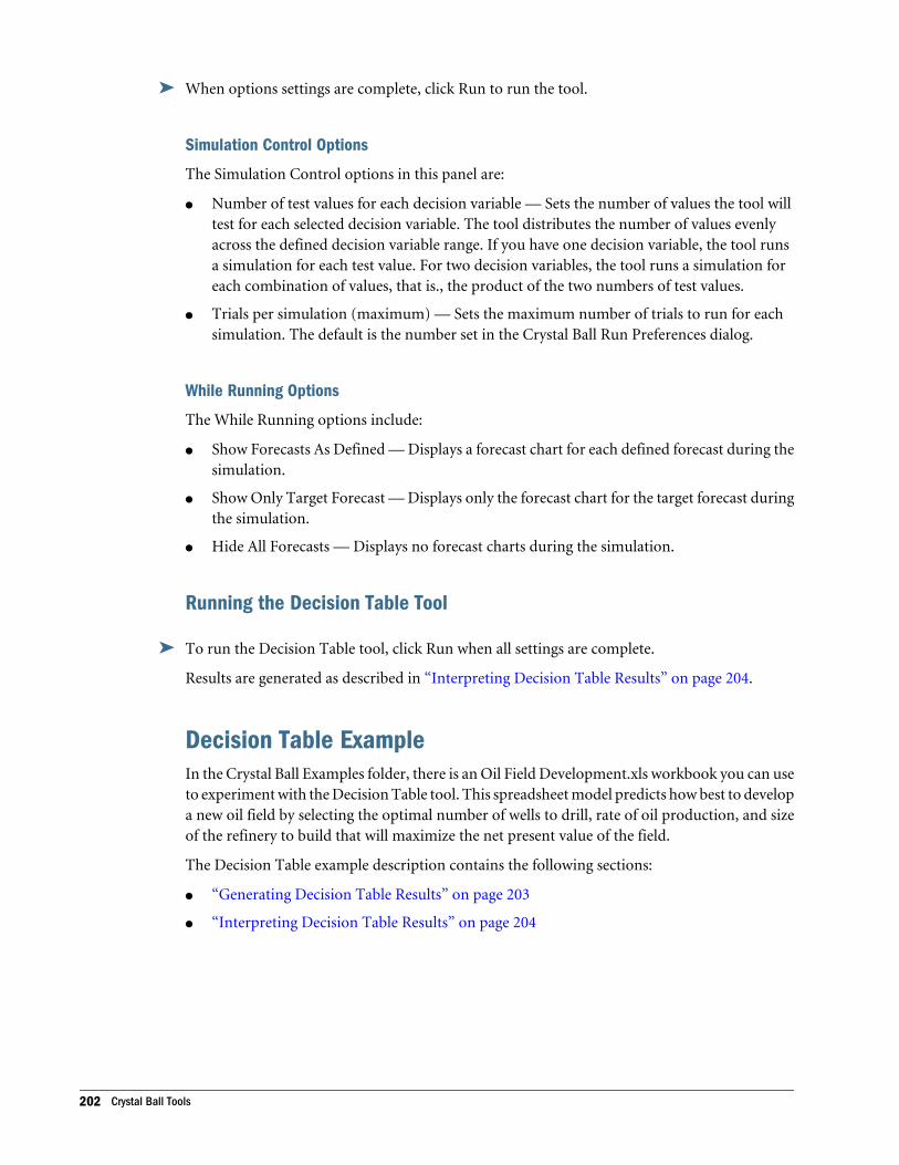
ä When options settings are complete, click Run to run the tool.
Simulation Control Options
The Simulation Control options in this panel are:
l Number of test values for each decision variable — Sets the number of values the tool willtest for each selected decision variable. The tool distributes the number of values evenlyacross the defined decision variable range. If you have one decision variable, the tool runsa simulation for each test value. For two decision variables, the tool runs a simulation foreach combination of values, that is., the product of the two numbers of test values.
l Trials per simulation (maximum) — Sets the maximum number of trials to run for eachsimulation. The default is the number set in the Crystal Ball Run Preferences dialog.
While Running Options
The While Running options include:
l Show Forecasts As Defined — Displays a forecast chart for each defined forecast during thesimulation.
l Show Only Target Forecast — Displays only the forecast chart for the target forecast duringthe simulation.
l Hide All Forecasts — Displays no forecast charts during the simulation.
Running the Decision Table Tool
ä To run the Decision Table tool, click Run when all settings are complete.
Results are generated as described in “Interpreting Decision Table Results” on page 204.
Decision Table ExampleIn the Crystal Ball Examples folder, there is an Oil Field Development.xls workbook you can useto experiment with the Decision Table tool. This spreadsheet model predicts how best to developa new oil field by selecting the optimal number of wells to drill, rate of oil production, and sizeof the refinery to build that will maximize the net present value of the field.
The Decision Table example description contains the following sections:
l “Generating Decision Table Results” on page 203
l “Interpreting Decision Table Results” on page 204
202 Crystal Ball Tools
Generating Decision Table Results
ä To run the Decision Table tool:
1 In Excel with Crystal Ball loaded, open the workbook Oil Field Development.xls.
2 In the Run, then Run Preferences, then Sampling dialog:
l Set Random Number Generation to use the Same Sequence Of Random Numbers and anInitial Seed Value of 999.
l Select Monte Carlo simulation.
When using this tool, use these options to make the resulting simulations comparable.
3 In the Run Preferences dialog, click OK.
4 Select Run, then More Tools, then Decision Table. (In Microsoft Excel 2007, select More Tools in the Toolsgroup.)
If this is the first time you have opened the Decision Table tool, the Welcome panel opens.
5 If the Welcome panel opens, click Next.
The Target Forecast panel opens.
6 Be sure the NPV forecast is selected and click Next.
The Decision Variables panel opens.
7 Move Facility Size and Wells To Drill to the Chosen Decision Variables list.
a. Press the Ctrl key and select Facility Size and Wells To Drill in the Available DecisionVariables list.
b. Click .
8 Click Next.
The Options panel opens, similar to Figure 75.
Decision Table Tool 203
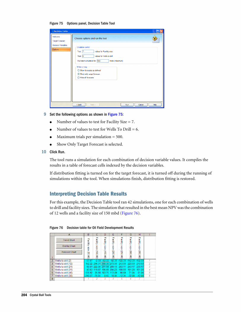
Figure 75 Options panel, Decision Table Tool
9 Set the following options as shown in Figure 75:
l Number of values to test for Facility Size = 7.
l Number of values to test for Wells To Drill = 6.
l Maximum trials per simulation = 500.
l Show Only Target Forecast is selected.
10 Click Run.
The tool runs a simulation for each combination of decision variable values. It compiles theresults in a table of forecast cells indexed by the decision variables.
If distribution fitting is turned on for the target forecast, it is turned off during the running ofsimulations within the tool. When simulations finish, distribution fitting is restored.
Interpreting Decision Table ResultsFor this example, the Decision Table tool ran 42 simulations, one for each combination of wellsto drill and facility sizes. The simulation that resulted in the best mean NPV was the combinationof 12 wells and a facility size of 150 mbd (Figure 76).
Figure 76 Decision table for Oil Field Development Results
204 Crystal Ball Tools
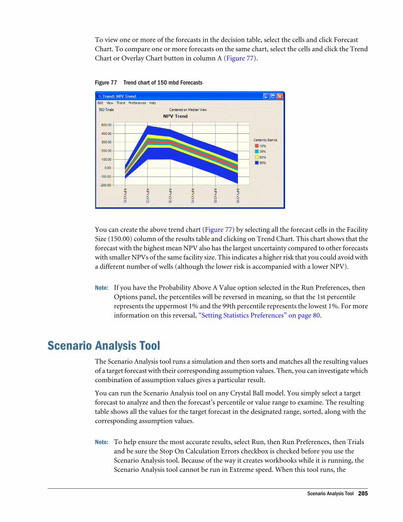
To view one or more of the forecasts in the decision table, select the cells and click ForecastChart. To compare one or more forecasts on the same chart, select the cells and click the TrendChart or Overlay Chart button in column A (Figure 77).
Figure 77 Trend chart of 150 mbd Forecasts
You can create the above trend chart (Figure 77) by selecting all the forecast cells in the FacilitySize (150.00) column of the results table and clicking on Trend Chart. This chart shows that theforecast with the highest mean NPV also has the largest uncertainty compared to other forecastswith smaller NPVs of the same facility size. This indicates a higher risk that you could avoid witha different number of wells (although the lower risk is accompanied with a lower NPV).
Note: If you have the Probability Above A Value option selected in the Run Preferences, thenOptions panel, the percentiles will be reversed in meaning, so that the 1st percentilerepresents the uppermost 1% and the 99th percentile represents the lowest 1%. For moreinformation on this reversal, “Setting Statistics Preferences” on page 80.
Scenario Analysis ToolThe Scenario Analysis tool runs a simulation and then sorts and matches all the resulting valuesof a target forecast with their corresponding assumption values. Then, you can investigate whichcombination of assumption values gives a particular result.
You can run the Scenario Analysis tool on any Crystal Ball model. You simply select a targetforecast to analyze and then the forecast’s percentile or value range to examine. The resultingtable shows all the values for the target forecast in the designated range, sorted, along with thecorresponding assumption values.
Note: To help ensure the most accurate results, select Run, then Run Preferences, then Trialsand be sure the Stop On Calculation Errors checkbox is checked before you use theScenario Analysis tool. Because of the way it creates workbooks while it is running, theScenario Analysis tool cannot be run in Extreme speed. When this tool runs, the
Scenario Analysis Tool 205
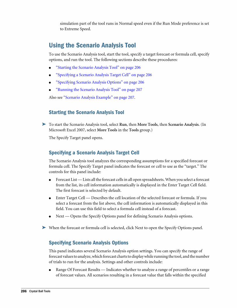
simulation part of the tool runs in Normal speed even if the Run Mode preference is setto Extreme Speed.
Using the Scenario Analysis ToolTo use the Scenario Analysis tool, start the tool, specify a target forecast or formula cell, specifyoptions, and run the tool. The following sections describe these procedures:
l “Starting the Scenario Analysis Tool” on page 206
l “Specifying a Scenario Analysis Target Cell” on page 206
l “Specifying Scenario Analysis Options” on page 206
l “Running the Scenario Analysis Tool” on page 207
Also see “Scenario Analysis Example” on page 207.
Starting the Scenario Analysis Tool
ä To start the Scenario Analysis tool, select Run, then More Tools, then Scenario Analysis. (InMicrosoft Excel 2007, select More Tools in the Tools group.)
The Specify Target panel opens.
Specifying a Scenario Analysis Target CellThe Scenario Analysis tool analyzes the corresponding assumptions for a specified forecast orformula cell. The Specify Target panel indicates the forecast or cell to use as the “target.” Thecontrols for this panel include:
l Forecast List — Lists all the forecast cells in all open spreadsheets. When you select a forecastfrom the list, its cell information automatically is displayed in the Enter Target Cell field.The first forecast is selected by default.
l Enter Target Cell — Describes the cell location of the selected forecast or formula. If youselect a forecast from the list above, the cell information is automatically displayed in thisfield. You can use this field to select a formula cell instead of a forecast.
l Next — Opens the Specify Options panel for defining Scenario Analysis options.
ä When the forecast or formula cell is selected, click Next to open the Specify Options panel.
Specifying Scenario Analysis OptionsThis panel indicates several Scenario Analysis option settings. You can specify the range offorecast values to analyze, which forecast charts to display while running the tool, and the numberof trials to run for the analysis. Settings and other controls include:
l Range Of Forecast Results — Indicates whether to analyze a range of percentiles or a rangeof forecast values. All scenarios resulting in a forecast value that falls within the specified
206 Crystal Ball Tools
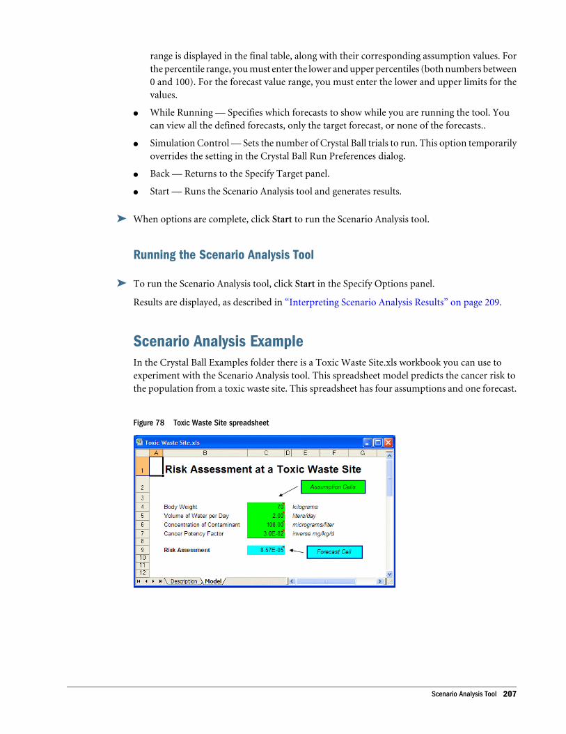
range is displayed in the final table, along with their corresponding assumption values. Forthe percentile range, you must enter the lower and upper percentiles (both numbers between0 and 100). For the forecast value range, you must enter the lower and upper limits for thevalues.
l While Running — Specifies which forecasts to show while you are running the tool. Youcan view all the defined forecasts, only the target forecast, or none of the forecasts..
l Simulation Control — Sets the number of Crystal Ball trials to run. This option temporarilyoverrides the setting in the Crystal Ball Run Preferences dialog.
l Back — Returns to the Specify Target panel.
l Start — Runs the Scenario Analysis tool and generates results.
ä When options are complete, click Start to run the Scenario Analysis tool.
Running the Scenario Analysis Tool
ä To run the Scenario Analysis tool, click Start in the Specify Options panel.
Results are displayed, as described in “Interpreting Scenario Analysis Results” on page 209.
Scenario Analysis ExampleIn the Crystal Ball Examples folder there is a Toxic Waste Site.xls workbook you can use toexperiment with the Scenario Analysis tool. This spreadsheet model predicts the cancer risk tothe population from a toxic waste site. This spreadsheet has four assumptions and one forecast.
Figure 78 Toxic Waste Site spreadsheet
Scenario Analysis Tool 207
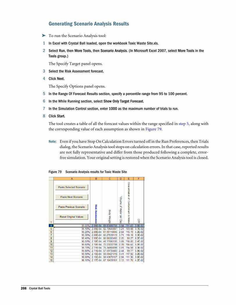
Generating Scenario Analysis Results
ä To run the Scenario Analysis tool:
1 In Excel with Crystal Ball loaded, open the workbook Toxic Waste Site.xls.
2 Select Run, then More Tools, then Scenario Analysis. (In Microsoft Excel 2007, select More Tools in theTools group.)
The Specify Target panel opens.
3 Select the Risk Assessment forecast.
4 Click Next.
The Specify Options panel opens.
5 In the Range Of Forecast Results section, specify a percentile range from 95 to 100 percent.
6 In the While Running section, select Show Only Target Forecast.
7 In the Simulation Control section, enter 1000 as the maximum number of trials to run.
8 Click Start.
The tool creates a table of all the forecast values within the range specified in step 5, along withthe corresponding value of each assumption as shown in Figure 79.
Note: Even if you have Stop On Calculation Errors turned off in the Run Preferences, then Trialsdialog, the Scenario Analysis tool stops on calculation errors. In that case, reported resultsare not fully representative and differ from those produced following a complete, error-free simulation. Your original setting is restored when the Scenario Analysis tool is closed.
Figure 79 Scenario Analysis results for Toxic Waste Site
208 Crystal Ball Tools
Note: For the next few steps, you might want to arrange the windows in Excel vertically, so thatyou can see the results next to the original workbook.
9 Select the row with the 98.00% (assuming default percentile settings).
10 Click Paste Selected Scenario.
The scenario of assumption values that produced the 98th percentile value of the target forecastis displayed in the Toxic Waste workbook. Crystal Ball recalculates the workbook and updatesthe forecast cells.
11 Click Paste Next Scenario.
In the workbook, the assumption and forecast values change to the values for the next scenario(for 98.10%).
12 Click Reset Original Values.
The original assumption and forecast values are displayed in the workbook.
Interpreting Scenario Analysis ResultsIn this example, the simulation generated 1,000 forecast values. Since you selected to analyzethe percentiles from 95 to 100, the resulting table lists 51 forecast values, or the top 5% of theforecast range, including the endpoints. The table sorts the values from lowest to highest valueand also includes the assumption values that Crystal Ball generated for each trial.
If you have the Probability Above A Value option selected in the Run Preferences, then Optionspanel, the percentiles will be reversed in meaning, so that the 1st percentile represents theuppermost 1% and the 99th percentile represents the lowest 1%.
One way to analyze the Scenario Analysis results is to identify a particular forecast value and seewhat assumption values created that forecast value.
Another way to analyze the Scenario Analysis results is to generate a scatter chart with the data.For example, you might create a scatter chart comparing the risk assessment with the CPF, asshown below.
Scenario Analysis Tool 209
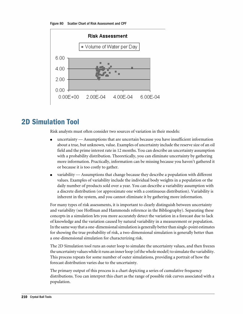
Figure 80 Scatter Chart of Risk Assessment and CPF
2D Simulation ToolRisk analysts must often consider two sources of variation in their models:
l uncertainty — Assumptions that are uncertain because you have insufficient informationabout a true, but unknown, value. Examples of uncertainty include the reserve size of an oilfield and the prime interest rate in 12 months. You can describe an uncertainty assumptionwith a probability distribution. Theoretically, you can eliminate uncertainty by gatheringmore information. Practically, information can be missing because you haven’t gathered itor because it is too costly to gather.
l variability — Assumptions that change because they describe a population with differentvalues. Examples of variability include the individual body weights in a population or thedaily number of products sold over a year. You can describe a variability assumption witha discrete distribution (or approximate one with a continuous distribution). Variability isinherent in the system, and you cannot eliminate it by gathering more information.
For many types of risk assessments, it is important to clearly distinguish between uncertaintyand variability (see Hoffman and Hammonds reference in the Bibliography). Separating theseconcepts in a simulation lets you more accurately detect the variation in a forecast due to lackof knowledge and the variation caused by natural variability in a measurement or population.In the same way that a one-dimensional simulation is generally better than single-point estimatesfor showing the true probability of risk, a two-dimensional simulation is generally better thana one-dimensional simulation for characterizing risk.
The 2D Simulation tool runs an outer loop to simulate the uncertainty values, and then freezesthe uncertainty values while it runs an inner loop (of the whole model) to simulate the variability.This process repeats for some number of outer simulations, providing a portrait of how theforecast distribution varies due to the uncertainty.
The primary output of this process is a chart depicting a series of cumulative frequencydistributions. You can interpret this chart as the range of possible risk curves associated with apopulation.
210 Crystal Ball Tools
Note: When using this tool, set the Seed Value option in the Crystal Ball Run Preferences dialogso that the resulting simulations are more comparable.
The following sections describe and show how to use the 2D Simulation tool and its results:
l “Using the 2D Simulation Tool” on page 211
l “2D Simulation Example” on page 213
l “Second-Order Assumptions” on page 218
Using the 2D Simulation ToolTo use the 2D Simulation tool, start the tool, select a forecast to analyze, sort assumptions intoUncertainty and Variability groups, set options, and run the tool. The following sections describethese procedures:
l “Starting the 2D Simulation Tool” on page 211
l “Using the 2D Simulation Welcome Panel” on page 211
l “Specifying a 2D Simulation Target Forecast” on page 212
l “Sorting Assumptions for 2D Simulation Analysis” on page 212
l “Setting 2D Simulation Options” on page 212
l “Running the 2D Simulation Tool” on page 213
Also see “2D Simulation Example” on page 213.
Starting the 2D Simulation Tool
ä To start the 2D Simulation tool, select Run, then More Tools, then 2D Simulation. (In MicrosoftExcel 2007, select More Tools in the Tools group.)
The first time you start 2D Simulation, the Welcome panel opens. Otherwise, the Target Forecastpanel opens.
Using the 2D Simulation Welcome PanelThe Welcome panel opens the first time you use the 2D Simulation tool. It describes the tooland its use. The controls for this panel include:
l Next — Opens the Target Forecast panel for specifying the forecast to analyze.
l Run — Runs the 2D Simulation tool if all required settings are complete.
2D Simulation Tool 211
ä If the Welcome panel opens, click Next to open the Target Forecast panel.
Specifying a 2D Simulation Target ForecastThe Target Forecast panel of the 2D Simulation tool indicates which forecast to analyze. Thecontrols for this panel include:
l Forecast list — Lists all the forecast cells in all open spreadsheets. The first forecast is selectedby default.
l Back — Opens the Welcome panel.
l Next — Opens the Assumption Types panel.
l Run — Runs the 2D Simulation tool if all required settings are complete.
ä When settings are complete on the Target Forecast panel, click Next to open the AssumptionTypes panel.
Sorting Assumptions for 2D Simulation AnalysisThe Assumption Types panel of the 2D Simulation tool separates the assumptions intouncertainty assumptions and variability assumptions. All the assumptions from all openworksheets start in the Uncertainty list by default. You must have at least one assumption ofeach type. When you save your spreadsheet model, the tool remembers the assumption typesfor the next time you run the tool. The controls for this panel include:
l >> — Moves any selected assumptions in the Uncertainty list to the Variability list.
l << — Moves any selected assumptions in the Variability list to the Uncertainty list.
l Back — Returns to the Target Forecast panel.
l Next — Opens the Options panel.
l Run — Runs the 2D Simulation tool if all required settings are complete.
ä When all assumptions have been sorted into the Uncertainty and Variability lists, click Next toopen the Options panel.
Setting 2D Simulation OptionsThe Options panel of the 2D Simulation tool sets simulation control, display, and report options.This panel includes the following controls:
l Simulation Control — Sets the number of trials for the outer (uncertainty) simulation andinner (variability) simulation. The default number of outer trials is 50 and the defaultnumber of inner trials is the number you have set on the Trials tab of the Run Preferencesdialog.
l While Running — Specifies which forecasts to show while you are running the tool. Youcan view the forecasts according to the display setting for each chart, only the target forecast,or none of the forecasts.
212 Crystal Ball Tools
l Report Options — Includes statistics, percentiles, and capability metrics in reports. You canalso specify how many simulations to include in accompanying output and overlay charts.
l Back — Opens the Assumption Types panel for identifying uncertainty and variabilityassumptions.
l Run — Runs the 2D Simulation tool if all required settings are complete.
ä When 2D Simulation tool settings are complete, click Run to run the tool and generate results,as shown in “Interpreting 2D Simulation Results” on page 214.
Running the 2D Simulation Tool
ä To run the 2D Simulation tool, confirm that all required settings are complete and then clickRun. Results are generated, as described in “Interpreting 2D Simulation Results” on page 214.
2D Simulation ExampleIn the Crystal Ball Examples folder there is a Toxic Waste Site.xls workbook you can use toexperiment with the 2D Simulation tool. This spreadsheet model predicts the cancer risk to thepopulation from a toxic waste site. This spreadsheet has two variability assumptions and twouncertainty assumptions.
The 2D Simulation tool example contains the following sections:
l “Interpreting 2D Simulation Results” on page 214
l “Interpreting 2D Simulation Results” on page 214
Generating 2D Simulation Results
ä To run the 2D Simulation tool:
1 In Excel with Crystal Ball loaded, open the workbook Toxic Waste Site.xls.
2 In the Run, then Run Preferences, then Sampling dialog:
l Set Random Number Generation to use the Same Sequence Of Random Numbers and AnInitial Seed Value of 999.
l Select Monte Carlo simulation.
When using this tool, use these options to make the resulting simulations comparable.
3 Select Run, then More Tools, then 2D Simulation. (In Microsoft Excel 2007, select More Tools in the Toolsgroup.)
If this is the first time you have opened the 2D Simulation tool, the Welcome panel opens.
4 If the Welcome panel opens, click Next.
The Target Forecast panel opens.
5 Be sure the Risk Assessment forecast is selected.
2D Simulation Tool 213
6 Click Next.
The Assumption Types panel opens.
7 Move Body Weight and Volume Of Water Per Day to the Variability list.
a. Select Body Weight.
b. Press Ctrl and then click Volume Of Water Per Day.
c. Click .
This separates the assumptions into the two types: Uncertainty and Variability.
8 Click Next.
The Options panel opens. The default number of trials for the outer (uncertainty) simulation is50. The default for the inner (variability) simulation is the number of trials currently set on theTrials tab of the Run Preferences dialog.
9 Set the following options.
l Run outer (uncertainty) simulation for 100 trials
l Run inner (variability) simulation for 1,000 trials
l Show Only Target Forecast is selected.
Use the default settings in the Report Options group.
10 Click Run.
The simulations start. The tool first single-steps one trial to generate a new set of values for theuncertainty assumptions. Then it freezes these assumptions and runs a simulation for thevariability assumptions in the inner loop.
The tool retrieves the Crystal Ball forecast information after each inner loop runs. The tool thenresets the simulation and repeats the process until the outer loop has run for the specified numberof simulations.
Interpreting 2D Simulation ResultsThe results of the simulations are displayed in a table containing the forecast means, theuncertainty assumption values, and the statistics (including percentiles) of the forecastdistribution for each simulation (Figure 81).
214 Crystal Ball Tools
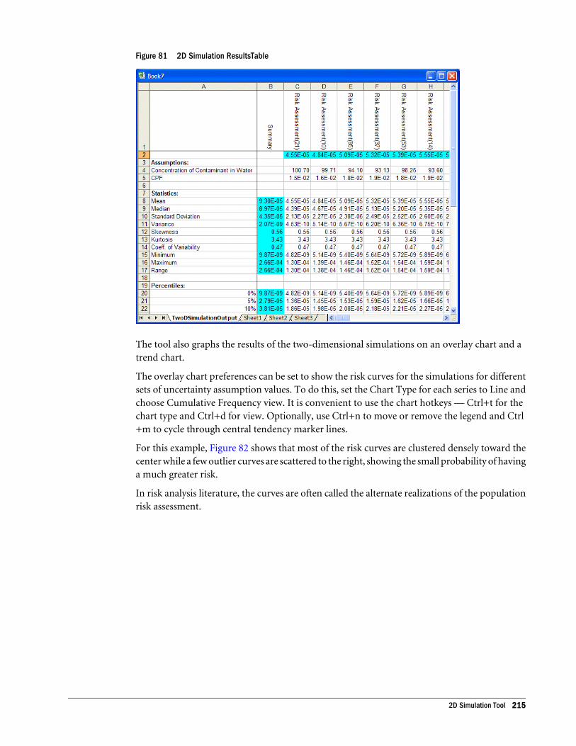
Figure 81 2D Simulation ResultsTable
The tool also graphs the results of the two-dimensional simulations on an overlay chart and atrend chart.
The overlay chart preferences can be set to show the risk curves for the simulations for differentsets of uncertainty assumption values. To do this, set the Chart Type for each series to Line andchoose Cumulative Frequency view. It is convenient to use the chart hotkeys — Ctrl+t for thechart type and Ctrl+d for view. Optionally, use Ctrl+n to move or remove the legend and Ctrl+m to cycle through central tendency marker lines.
For this example, Figure 82 shows that most of the risk curves are clustered densely toward thecenter while a few outlier curves are scattered to the right, showing the small probability of havinga much greater risk.
In risk analysis literature, the curves are often called the alternate realizations of the populationrisk assessment.
2D Simulation Tool 215
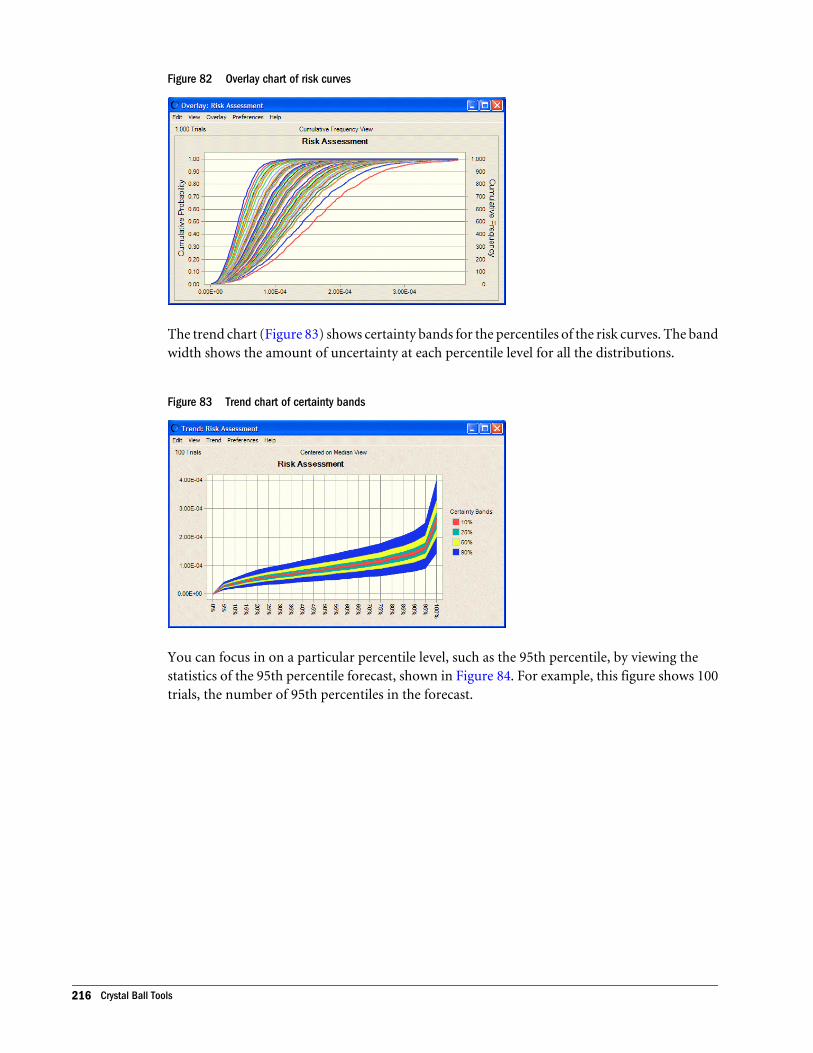
Figure 82 Overlay chart of risk curves
The trend chart (Figure 83) shows certainty bands for the percentiles of the risk curves. The bandwidth shows the amount of uncertainty at each percentile level for all the distributions.
Figure 83 Trend chart of certainty bands
You can focus in on a particular percentile level, such as the 95th percentile, by viewing thestatistics of the 95th percentile forecast, shown in Figure 84. For example, this figure shows 100trials, the number of 95th percentiles in the forecast.
216 Crystal Ball Tools

Figure 84 95th percentiles forecast statistics
If you have the Probability Above A Value option selected in the Run Preferences, then Optionspanel, the percentiles will be reversed in meaning, so that the 1st percentile represents theuppermost 1% and the 99th percentile represents the lowest 1%. For more information, see“Setting Statistics Preferences” on page 80.
Compare the results of the two-dimensional simulation to a one-dimensional simulation (withboth uncertainty and variability co-mingling together) of the same risk model, as in Figure 85,following .
The mean of the 95th percentiles in Figure 84, 1.45E-4, is lower than the 95th percentile risk ofthe one-dimensional simulation shown in Figure 85 at 2.06E-4. This indicates the tendency ofthe one-dimensional simulation results to overestimate the population risk, especially for highlyskewed distributions.
Figure 85 Forecast chart for one-dimensional simulation
2D Simulation Tool 217
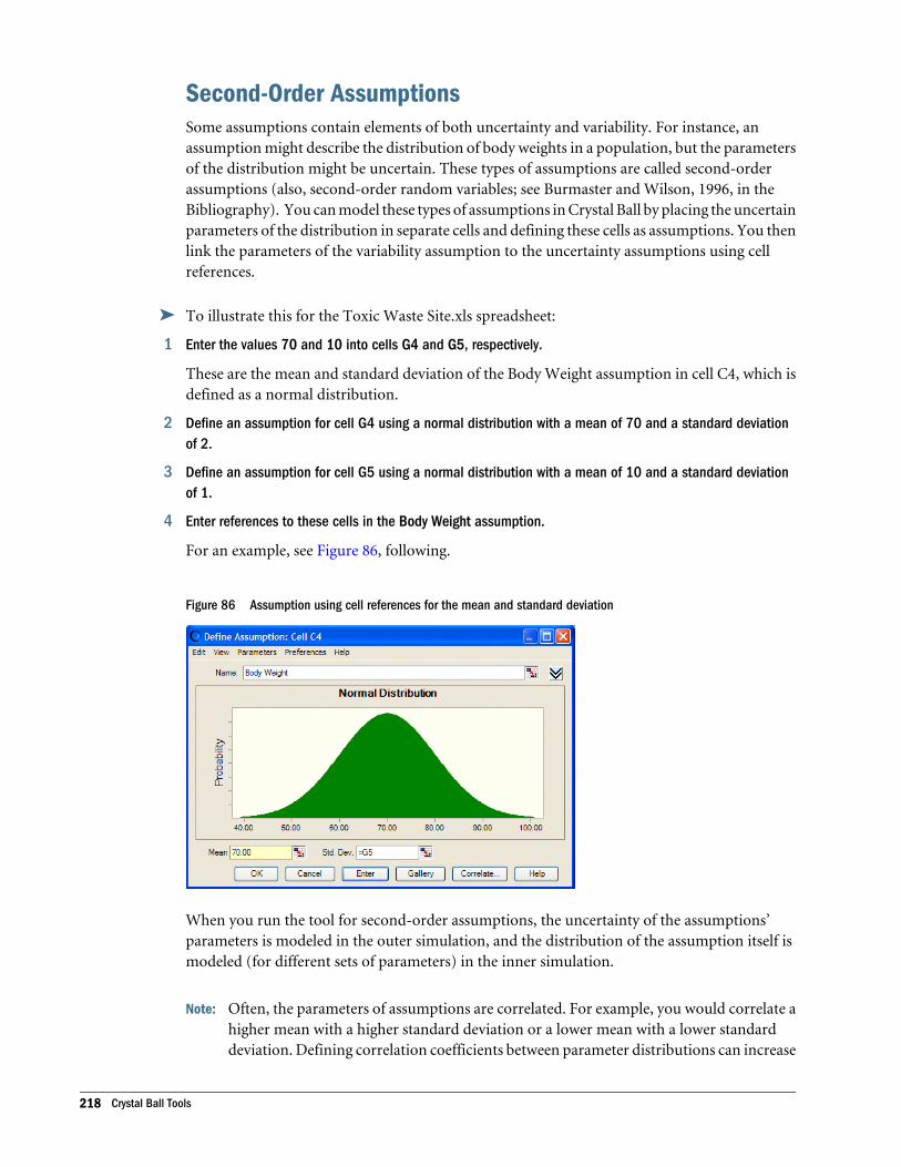
Second-Order AssumptionsSome assumptions contain elements of both uncertainty and variability. For instance, anassumption might describe the distribution of body weights in a population, but the parametersof the distribution might be uncertain. These types of assumptions are called second-orderassumptions (also, second-order random variables; see Burmaster and Wilson, 1996, in theBibliography). You can model these types of assumptions in Crystal Ball by placing the uncertainparameters of the distribution in separate cells and defining these cells as assumptions. You thenlink the parameters of the variability assumption to the uncertainty assumptions using cellreferences.
ä To illustrate this for the Toxic Waste Site.xls spreadsheet:
1 Enter the values 70 and 10 into cells G4 and G5, respectively.
These are the mean and standard deviation of the Body Weight assumption in cell C4, which isdefined as a normal distribution.
2 Define an assumption for cell G4 using a normal distribution with a mean of 70 and a standard deviationof 2.
3 Define an assumption for cell G5 using a normal distribution with a mean of 10 and a standard deviationof 1.
4 Enter references to these cells in the Body Weight assumption.
For an example, see Figure 86, following.
Figure 86 Assumption using cell references for the mean and standard deviation
When you run the tool for second-order assumptions, the uncertainty of the assumptions’parameters is modeled in the outer simulation, and the distribution of the assumption itself ismodeled (for different sets of parameters) in the inner simulation.
Note: Often, the parameters of assumptions are correlated. For example, you would correlate ahigher mean with a higher standard deviation or a lower mean with a lower standarddeviation. Defining correlation coefficients between parameter distributions can increase
218 Crystal Ball Tools
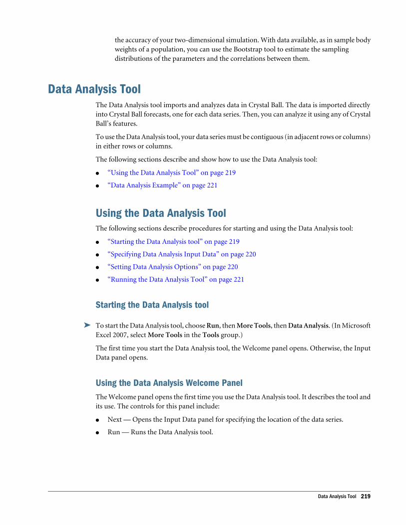
the accuracy of your two-dimensional simulation. With data available, as in sample bodyweights of a population, you can use the Bootstrap tool to estimate the samplingdistributions of the parameters and the correlations between them.
Data Analysis ToolThe Data Analysis tool imports and analyzes data in Crystal Ball. The data is imported directlyinto Crystal Ball forecasts, one for each data series. Then, you can analyze it using any of CrystalBall’s features.
To use the Data Analysis tool, your data series must be contiguous (in adjacent rows or columns)in either rows or columns.
The following sections describe and show how to use the Data Analysis tool:
l “Using the Data Analysis Tool” on page 219
l “Data Analysis Example” on page 221
Using the Data Analysis ToolThe following sections describe procedures for starting and using the Data Analysis tool:
l “Starting the Data Analysis tool” on page 219
l “Specifying Data Analysis Input Data” on page 220
l “Setting Data Analysis Options” on page 220
l “Running the Data Analysis Tool” on page 221
Starting the Data Analysis tool
ä To start the Data Analysis tool, choose Run, then More Tools, then Data Analysis. (In MicrosoftExcel 2007, select More Tools in the Tools group.)
The first time you start the Data Analysis tool, the Welcome panel opens. Otherwise, the InputData panel opens.
Using the Data Analysis Welcome PanelThe Welcome panel opens the first time you use the Data Analysis tool. It describes the tool andits use. The controls for this panel include:
l Next — Opens the Input Data panel for specifying the location of the data series.
l Run — Runs the Data Analysis tool.
Data Analysis Tool 219
ä If the Welcome panel opens, click Next to open the Input Data panel.
Specifying Data Analysis Input DataThe Input Data panel of the Data Analysis tool indicates the location of the data that to analyze.You can also set input-related options. The Data Analysis data selector chooses possible data forfitting. This information is displayed in the Location Of Data Series field and the illustration atthe right side of the panel. You can choose different data if necessary. The controls in this panelinclude:
l Location Of Data Series — Indicates the cells that contain data to analyze. If your data hasheaders or labels at the beginning of the rows or columns of data, include them in yourselection and select the appropriate Headers setting(s). The data must be in adjacent rowsor columns.
l Orientation — Sets whether your data is in rows or columns: Data In Rows indicates thatdata is in horizontal rows; Data In Columns indicates that data is in vertical columns.
l Headers — Indicates whether your data has headers and/or labels and whether they arelocated in the top row or the left header (varies with orientation). Checked items are usedin the output: Top Row Has Headers/Labels includes text in the top row in your selection;Left Column Has Labels/Headers includes text in the left column in your selection.
l Back — Returns to the Welcome panel.
l Next — Opens the Options panel.
l Run — Runs the Data Analysis tool, automatically generating forecasts for each selecteddata series.
ä Click Next to open the Options panel and set Data Analysis options.
Setting Data Analysis OptionsThe Options panel of the Data Analysis tool sets a variety of preferences for displaying generatedforecast charts, fitting probability distributions to generated forecast data, generatingcorrelations between forecast data series, and running simulations on opened models. TheOptions panel includes these controls:
l Automatically Open Forecast Charts — When checked, automatically opens forecast chartswhen the Data Analysis tool runs.
l View — Indicates which forecast chart view to use, similar to the forecast chart View menucommands.
l Split View — When checked, shows a chart in the left pane and statistics in the right pane.
l Fit A Probability Distribution To The Data — When checked, calculates and plots a curvefor the distribution that best fits the data in each series. Select Fit Options to review or changecurrent settings in the Fit Options panel.
l Generate Correlation Matrix Between Data Series — When checked, plots the rankcorrelation between pairs of forecasts. You can click the Scatter Chart button in the results
220 Crystal Ball Tools
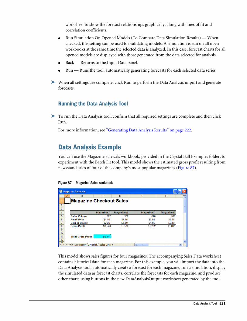
worksheet to show the forecast relationships graphically, along with lines of fit andcorrelation coefficients.
l Run Simulation On Opened Models (To Compare Data Simulation Results) — Whenchecked, this setting can be used for validating models. A simulation is run on all openworkbooks at the same time the selected data is analyzed. In this case, forecast charts for allopened models are displayed with those generated from the data selected for analysis.
l Back — Returns to the Input Data panel.
l Run — Runs the tool, automatically generating forecasts for each selected data series.
ä When all settings are complete, click Run to perform the Data Analysis import and generateforecasts.
Running the Data Analysis Tool
ä To run the Data Analysis tool, confirm that all required settings are complete and then clickRun.
For more information, see “Generating Data Analysis Results” on page 222.
Data Analysis ExampleYou can use the Magazine Sales.xls workbook, provided in the Crystal Ball Examples folder, toexperiment with the Batch Fit tool. This model shows the estimated gross profit resulting fromnewsstand sales of four of the company’s most popular magazines (Figure 87).
Figure 87 Magazine Sales workbook
This model shows sales figures for four magazines. The accompanying Sales Data worksheetcontains historical data for each magazine. For this example, you will import the data into theData Analysis tool, automatically create a forecast for each magazine, run a simulation, displaythe simulated data as forecast charts, correlate the forecasts for each magazine, and produceother charts using buttons in the new DataAnalysisOutput worksheet generated by the tool.
Data Analysis Tool 221
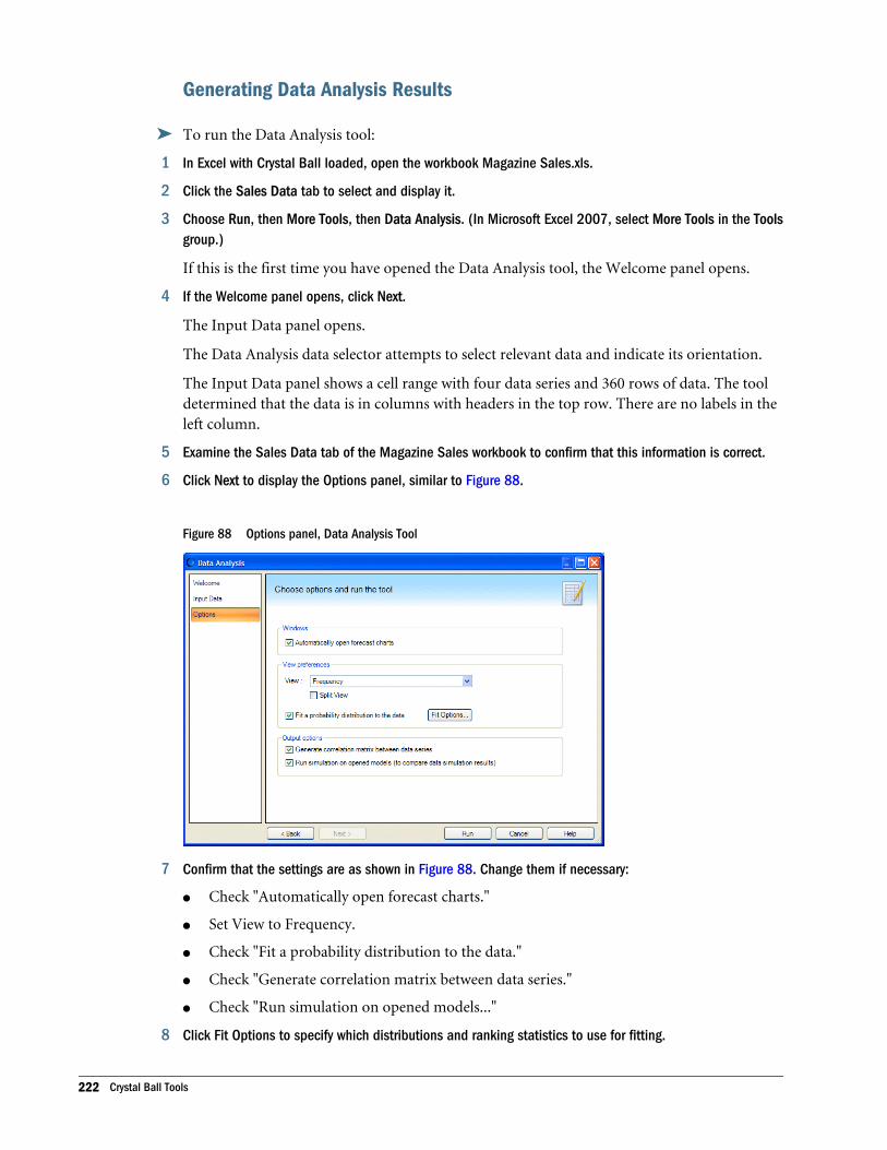
Generating Data Analysis Results
ä To run the Data Analysis tool:
1 In Excel with Crystal Ball loaded, open the workbook Magazine Sales.xls.
2 Click the Sales Data tab to select and display it.
3 Choose Run, then More Tools, then Data Analysis. (In Microsoft Excel 2007, select More Tools in the Toolsgroup.)
If this is the first time you have opened the Data Analysis tool, the Welcome panel opens.
4 If the Welcome panel opens, click Next.
The Input Data panel opens.
The Data Analysis data selector attempts to select relevant data and indicate its orientation.
The Input Data panel shows a cell range with four data series and 360 rows of data. The tooldetermined that the data is in columns with headers in the top row. There are no labels in theleft column.
5 Examine the Sales Data tab of the Magazine Sales workbook to confirm that this information is correct.
6 Click Next to display the Options panel, similar to Figure 88.
Figure 88 Options panel, Data Analysis Tool
7 Confirm that the settings are as shown in Figure 88. Change them if necessary:
l Check "Automatically open forecast charts."
l Set View to Frequency.
l Check "Fit a probability distribution to the data."
l Check "Generate correlation matrix between data series."
l Check "Run simulation on opened models..."
8 Click Fit Options to specify which distributions and ranking statistics to use for fitting.
222 Crystal Ball Tools
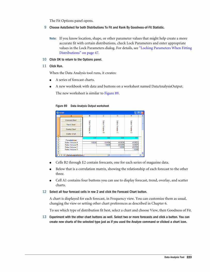
The Fit Options panel opens.
9 Choose AutoSelect for both Distributions To Fit and Rank By Goodness-of-Fit Statistic.
Note: If you know location, shape, or other parameter values that might help create a moreaccurate fit with certain distributions, check Lock Parameters and enter appropriatevalues in the Lock Parameters dialog. For details, see “Locking Parameters When FittingDistributions” on page 47.
10 Click OK to return to the Options panel.
11 Click Run.
When the Data Analysis tool runs, it creates:
l A series of forecast charts.
l A new workbook with data and buttons on a worksheet named DataAnalysisOutput.
The new worksheet is similar to Figure 89.
Figure 89 Data Analysis Output worksheet
l Cells B2 through E2 contain forecasts, one for each series of magazine data.
l Below that is a correlation matrix, showing the relationship of each forecast to the otherthree.
l Cell A1 contains four buttons you can use to display forecast, trend, overlay, and scattercharts.
12 Select all four forecast cells in row 2 and click the Forecast Chart button.
A chart is displayed for each forecast, in Frequency view. You can customize them as usual,changing the view or setting other chart preferences as described in Chapter 6.
To see which type of distribution fit best, select a chart and choose View, then Goodness of Fit.
13 Experiment with the other chart buttons as well. Select two or more forecasts and click a button. You cancreate new charts of the selected type just as if you used the Analyze command or clicked a chart icon.
Data Analysis Tool 223

224 Crystal Ball Tools
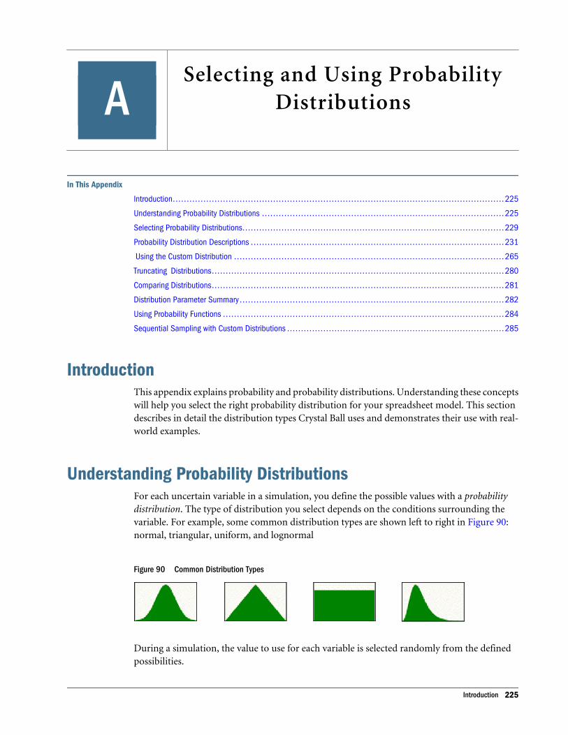
ASelecting and Using Probability
Distributions
In This Appendix
Introduction... . . . . . . . . . . . . . . . . . . . . . . . . . . . . . . . . . . . . . . . . . . . . . . . . . . . . . . . . . . . . . . . . . . . . . . . . . . . . . . . . . . . . . . . . . . . . . . . . . . . . . . . . . . . . . . . . . . . . 225
Understanding Probability Distributions ... . . . . . . . . . . . . . . . . . . . . . . . . . . . . . . . . . . . . . . . . . . . . . . . . . . . . . . . . . . . . . . . . . . . . . . . . . . . . . . . . . . . . 225
Selecting Probability Distributions... . . . . . . . . . . . . . . . . . . . . . . . . . . . . . . . . . . . . . . . . . . . . . . . . . . . . . . . . . . . . . . . . . . . . . . . . . . . . . . . . . . . . . . . . . . . 229
Probability Distribution Descriptions ... . . . . . . . . . . . . . . . . . . . . . . . . . . . . . . . . . . . . . . . . . . . . . . . . . . . . . . . . . . . . . . . . . . . . . . . . . . . . . . . . . . . . . . . . 231
Using the Custom Distribution ... . . . . . . . . . . . . . . . . . . . . . . . . . . . . . . . . . . . . . . . . . . . . . . . . . . . . . . . . . . . . . . . . . . . . . . . . . . . . . . . . . . . . . . . . . . . . . . 265
Truncating Distributions... . . . . . . . . . . . . . . . . . . . . . . . . . . . . . . . . . . . . . . . . . . . . . . . . . . . . . . . . . . . . . . . . . . . . . . . . . . . . . . . . . . . . . . . . . . . . . . . . . . . . . . 280
Comparing Distributions... . . . . . . . . . . . . . . . . . . . . . . . . . . . . . . . . . . . . . . . . . . . . . . . . . . . . . . . . . . . . . . . . . . . . . . . . . . . . . . . . . . . . . . . . . . . . . . . . . . . . . . 281
Distribution Parameter Summary ... . . . . . . . . . . . . . . . . . . . . . . . . . . . . . . . . . . . . . . . . . . . . . . . . . . . . . . . . . . . . . . . . . . . . . . . . . . . . . . . . . . . . . . . . . . . . 282
Using Probability Functions ... . . . . . . . . . . . . . . . . . . . . . . . . . . . . . . . . . . . . . . . . . . . . . . . . . . . . . . . . . . . . . . . . . . . . . . . . . . . . . . . . . . . . . . . . . . . . . . . . . . 284
Sequential Sampling with Custom Distributions ... . . . . . . . . . . . . . . . . . . . . . . . . . . . . . . . . . . . . . . . . . . . . . . . . . . . . . . . . . . . . . . . . . . . . . . . . . . . 285
IntroductionThis appendix explains probability and probability distributions. Understanding these conceptswill help you select the right probability distribution for your spreadsheet model. This sectiondescribes in detail the distribution types Crystal Ball uses and demonstrates their use with real-world examples.
Understanding Probability DistributionsFor each uncertain variable in a simulation, you define the possible values with a probabilitydistribution. The type of distribution you select depends on the conditions surrounding thevariable. For example, some common distribution types are shown left to right in Figure 90:normal, triangular, uniform, and lognormal
Figure 90 Common Distribution Types
During a simulation, the value to use for each variable is selected randomly from the definedpossibilities.
Introduction 225
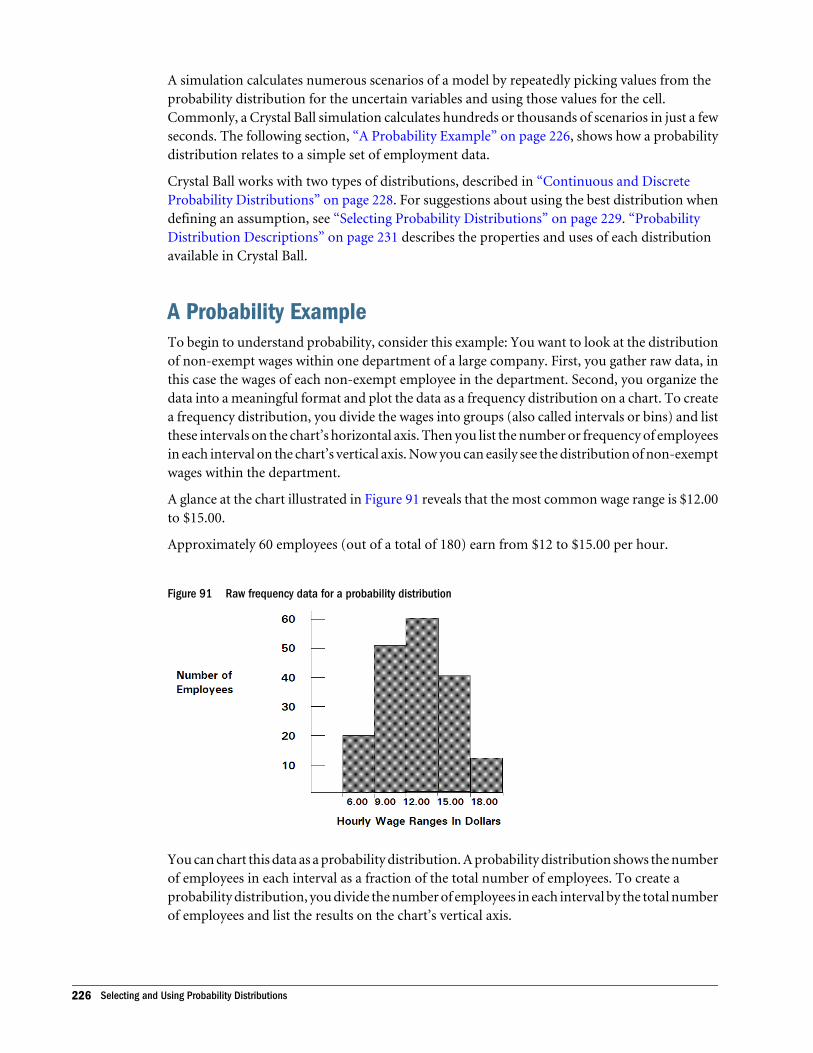
A simulation calculates numerous scenarios of a model by repeatedly picking values from theprobability distribution for the uncertain variables and using those values for the cell.Commonly, a Crystal Ball simulation calculates hundreds or thousands of scenarios in just a fewseconds. The following section, “A Probability Example” on page 226, shows how a probabilitydistribution relates to a simple set of employment data.
Crystal Ball works with two types of distributions, described in “Continuous and DiscreteProbability Distributions” on page 228. For suggestions about using the best distribution whendefining an assumption, see “Selecting Probability Distributions” on page 229. “ProbabilityDistribution Descriptions” on page 231 describes the properties and uses of each distributionavailable in Crystal Ball.
A Probability ExampleTo begin to understand probability, consider this example: You want to look at the distributionof non-exempt wages within one department of a large company. First, you gather raw data, inthis case the wages of each non-exempt employee in the department. Second, you organize thedata into a meaningful format and plot the data as a frequency distribution on a chart. To createa frequency distribution, you divide the wages into groups (also called intervals or bins) and listthese intervals on the chart’s horizontal axis. Then you list the number or frequency of employeesin each interval on the chart’s vertical axis. Now you can easily see the distribution of non-exemptwages within the department.
A glance at the chart illustrated in Figure 91 reveals that the most common wage range is $12.00to $15.00.
Approximately 60 employees (out of a total of 180) earn from $12 to $15.00 per hour.
Figure 91 Raw frequency data for a probability distribution
You can chart this data as a probability distribution. A probability distribution shows the numberof employees in each interval as a fraction of the total number of employees. To create aprobability distribution, you divide the number of employees in each interval by the total numberof employees and list the results on the chart’s vertical axis.
226 Selecting and Using Probability Distributions
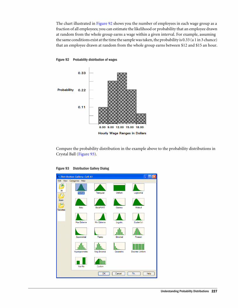
The chart illustrated in Figure 92 shows you the number of employees in each wage group as afraction of all employees; you can estimate the likelihood or probability that an employee drawnat random from the whole group earns a wage within a given interval. For example, assumingthe same conditions exist at the time the sample was taken, the probability is 0.33 (a 1 in 3 chance)that an employee drawn at random from the whole group earns between $12 and $15 an hour.
Figure 92 Probability distribution of wages
Compare the probability distribution in the example above to the probability distributions inCrystal Ball (Figure 93).
Figure 93 Distribution Gallery Dialog
Understanding Probability Distributions 227
The probability distribution in the example in Figure 92 has a shape similar to many of thedistributions in the Distribution Gallery. This process of plotting data as a frequency distributionand converting it to a probability distribution provides one starting point for selecting a CrystalBall distribution. Select the distributions in the gallery that is displayed similar to your probabilitydistribution, then read about those distributions in this chapter to find the correct distribution.
For information about the similarities between distributions, see “Comparing Distributions”on page 281. For a complete discussion of probability distributions, refer to the sources listedin the bibliography.
Continuous and Discrete Probability DistributionsNotice that the Distribution Gallery shows whether the probability distributions are continuousor discrete.
Continuous probability distributions, such as the normal distribution, describe values over arange or scale and are shown as solid figures in the Distribution Gallery. Continuousdistributions are actually mathematical abstractions because they assume the existence of everypossible intermediate value between two numbers. That is, a continuous distribution assumesthere is an infinite number of values between any two points in the distribution.
Discrete probability distributions describe distinct values, usually integers, with no intermediatevalues and are shown as a series of vertical columns, such as the binomial distribution at thebottom of Figure 93. A discrete distribution, for example, might describe the number of headsin four flips of a coin as 0, 1, 2, 3, or 4.
However, in many situations, you can effectively use a continuous distribution to approximatea discrete distribution even though the continuous model does not necessarily describe thesituation exactly.
In the dialogs for the discrete distributions, Crystal Ball displays the values of the variable on thehorizontal axis and the associated probabilities on the vertical axis. For the continuousdistributions, Crystal Ball does not display values on the vertical axis since, in this case,probability can only be associated with areas under the curve and not with single values.
Initially, the precision and format of the displayed numbers in the probability and frequencydistributions come from the cell itself. To change the format, see “Customizing Chart Axes andAxis Labels” on page 120.
The following sections list continuous and discrete distributions available in Crystal Ball:
l “Continuous Probability Distributions” on page 228
l “Discrete Probability Distributions” on page 229
Note: Custom distributions can be defined as continuous, discrete, or both. For moreinformation, see “Custom Distribution” on page 236.
Continuous Probability DistributionsThe following sections describe continuous distributions available in Crystal Ball:
228 Selecting and Using Probability Distributions
l “Beta Distribution” on page 231
l “BetaPERT Distribution” on page 233
l “Exponential Distribution” on page 238
l “Gamma Distribution” on page 240
l “Logistic Distribution” on page 247
l “Lognormal Distribution” on page 248
l “Maximum Extreme Distribution” on page 250
l “Minimum Extreme Distribution” on page 251
l “Normal Distribution” on page 253
l “Pareto Distribution” on page 255
l “Student’s t Distribution” on page 258
l “Triangular Distribution” on page 259
l “Uniform Distribution” on page 261
l “Weibull Distribution” on page 262
Discrete Probability DistributionsThe following sections describe discrete distributions available in Crystal Ball:
l “Binomial Distribution” on page 235
l “Discrete Uniform Distribution” on page 237
l “Geometric Distribution” on page 243
l “Hypergeometric Distribution” on page 245
l “Negative Binomial Distribution” on page 252
l “Poisson Distribution” on page 256
l “Yes-No Distribution” on page 264
l “Triangular Distribution” on page 259
l “Uniform Distribution” on page 261
l “Weibull Distribution” on page 262
Selecting Probability DistributionsPlotting data is one guide to selecting a probability distribution. The following steps provideanother process for selecting probability distributions that best describe the uncertain variablesin your spreadsheets.
To select the correct probability distribution:
1. Look at the variable in question. List everything you know about the conditions surroundingthis variable.
Selecting Probability Distributions 229
You might be able to gather valuable information about the uncertain variable fromhistorical data. If historical data are not available, use your own judgment, based onexperience, to list everything you know about the uncertain variable.
For example, look at the variable "patients cured" that is discussed in “Tutorial 2 — VisionResearch” on page 333. The company plans to test 100 patients. You know that the patientswill either be cured or not cured. And, you know that the drug has shown a cure rate ofaround 0.25 (25%). These facts are the conditions surrounding the variable.
2. Review the descriptions of the probability distributions.
“Probability Distribution Descriptions” on page 231 describes each distribution in detail,outlining the conditions underlying the distribution and providing real-world examples ofeach distribution type. As you review the descriptions, look for a distribution that featuresthe conditions you have listed for this variable.
3. Select the distribution that characterizes this variable.
A distribution characterizes a variable when the conditions of the distribution match thoseof the variable.
The conditions of the variable describe the values for the parameters of the distribution inCrystal Ball. Each distribution type has its own set of parameters, which are explained in thefollowing descriptions.
For example, look at the conditions of the binomial distribution, as described in “BinomialDistribution” on page 235:
l For each trial, only two outcomes are possible: success or failure.
l The trials are independent. What happens on the first trial does not affect the secondtrial, and so on.
l The probability of success remains the same from trial to trial.
Now check the "patients cured" variable in Tutorial 2 in the Crystal Ball Getting StartedGuide against the conditions of the binomial distribution:
l There are two possible outcomes: the patient is either cured or not cured.
l The trials (100) are independent of each other. What happens to the first patient doesnot affect the second patient.
l The probability of curing a patient 0.25 (25%) remains the same each time a patient istested.
Since the conditions of the variable match the conditions of the binomial distribution,the binomial distribution would be the correct distribution type for the variable inquestion.
4. If historical data are available, use distribution fitting to select the distribution that bestdescribes your data.
Crystal Ball can automatically select the probability distribution that most closelyapproximates your data’s distribution. The feature is described in detail in “FittingDistributions to Data” on page 44. You can also populate a custom distribution with yourhistorical data.
230 Selecting and Using Probability Distributions
After you select a distribution type, determine the parameter values for the distribution.Each distribution type has its own set of parameters. For example, there are two parametersfor the binomial distribution: trials and probability. The conditions of a variable containthe values for the parameters. In the example used, the conditions show 100 trials and 0.25(25%) probability of success.
In addition to the standard parameter set, each continuous distribution (except uniform) alsolets you choose from alternate parameter sets, which substitute percentiles for one or more ofthe standard parameters. For more information on alternate parameters, see “AlternateParameter Sets” on page 43.
Probability Distribution DescriptionsThis section contains descriptions of all the Crystal Ball probability distributions, listed inalphabetical order.
The following sections list continuous and discrete distributions described below:
l “Continuous Probability Distributions” on page 228
l “Discrete Probability Distributions” on page 229
See “Custom Distribution” on page 236 for a description of the Custom distribution, which canbe continuous, discrete, or both
As you work with the Crystal Ball probability distributions, you can use the Parameters menufound in the distribution menubar to specify different combinations of parameters. For moreinformation, see “Alternate Parameter Sets” on page 43.
Beta Distribution
The beta distribution is continuous. It is commonly used to represent variability over a fixedrange. It can represent uncertainty in the probability of occurrence of an event. It is also usedto describe empirical data and predict the random behavior of percentages and fractions andcan be used to represent the reliability of a company’s devices.
The following sections describe the parameters, conditions, and other features of thisdistribution:
l “Beta Distribution Parameters” on page 231
l “Beta Distribution Conditions” on page 232
l “Beta Distribution Example” on page 232
Beta Distribution ParametersMinimum, Maximum, Alpha, Beta
Probability Distribution Descriptions 231
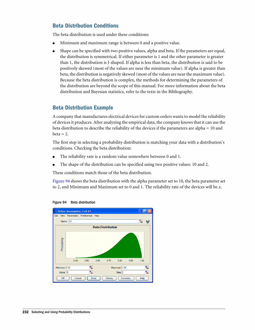
Beta Distribution ConditionsThe beta distribution is used under these conditions:
l Minimum and maximum range is between 0 and a positive value.
l Shape can be specified with two positive values, alpha and beta. If the parameters are equal,the distribution is symmetrical. If either parameter is 1 and the other parameter is greaterthan 1, the distribution is J-shaped. If alpha is less than beta, the distribution is said to bepositively skewed (most of the values are near the minimum value). If alpha is greater thanbeta, the distribution is negatively skewed (most of the values are near the maximum value).Because the beta distribution is complex, the methods for determining the parameters ofthe distribution are beyond the scope of this manual. For more information about the betadistribution and Bayesian statistics, refer to the texts in the Bibliography.
Beta Distribution ExampleA company that manufactures electrical devices for custom orders wants to model the reliabilityof devices it produces. After analyzing the empirical data, the company knows that it can use thebeta distribution to describe the reliability of the devices if the parameters are alpha = 10 andbeta = 2.
The first step in selecting a probability distribution is matching your data with a distribution’sconditions. Checking the beta distribution:
l The reliability rate is a random value somewhere between 0 and 1.
l The shape of the distribution can be specified using two positive values: 10 and 2.
These conditions match those of the beta distribution.
Figure 94 shows the beta distribution with the alpha parameter set to 10, the beta parameter setto 2, and Minimum and Maximum set to 0 and 1. The reliability rate of the devices will be x.
Figure 94 Beta distribution
232 Selecting and Using Probability Distributions
Models that use beta distributions will run more slowly because of the inverse CDF and alternateparameter calculations that take place when random numbers are handled as part of betadistributions.
BetaPERT Distribution
The betaPERT distribution is continuous. It describes a situation where you know the minimum,maximum, and most likely values to occur. It is useful with limited data. For example, you coulddescribe the number of cars sold per week when past sales show the minimum, maximum, andusual number of cars sold. It is similar to the triangular distribution, described in “TriangularDistribution” on page 259, except the curve is smoothed to reduce the peak. The betaPERTdistribution is often used in project management models to estimate task and project durations.
The following sections describe the parameters, conditions, and other features of thisdistribution:
l “BetaPERT Parameters” on page 233
l “BetaPERT Conditions” on page 233
l “BetaPERT Example” on page 233
BetaPERT ParametersMinimum, Likeliest, Maximum
BetaPERT ConditionsThe betaPERT distributions is used under these conditions:
l Minimum and maximum are fixed.
l It has a most likely value in this range, which forms a triangle with the minimum andmaximum; betaPERT forms a smoothed curve on the underlying triangle.
BetaPERT ExampleA project manager wants to estimate the time (number of days) required for completion of aproject. From the manager's past experience, similar projects typically take 7 days to finish, butcan be finished in 5 days given favorable conditions, and can take as long as 12 days if things donot happen as expected. The project manager wants to estimate the probability of finishingwithin 9 days.
The first step in selecting a probability distribution is matching available data with a distribution'sconditions. Checking the betaPERT distribution for this project:
Probability Distribution Descriptions 233
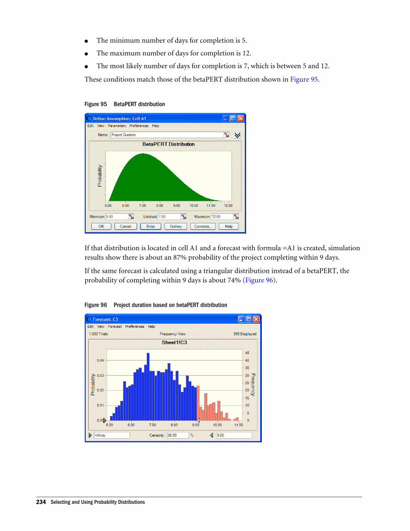
l The minimum number of days for completion is 5.
l The maximum number of days for completion is 12.
l The most likely number of days for completion is 7, which is between 5 and 12.
These conditions match those of the betaPERT distribution shown in Figure 95.
Figure 95 BetaPERT distribution
If that distribution is located in cell A1 and a forecast with formula =A1 is created, simulationresults show there is about an 87% probability of the project completing within 9 days.
If the same forecast is calculated using a triangular distribution instead of a betaPERT, theprobability of completing within 9 days is about 74% (Figure 96).
Figure 96 Project duration based on betaPERT distribution
234 Selecting and Using Probability Distributions
Binomial Distribution
The binomial distribution is discrete. It describes the number of times a particular event occursor fails to occur in a fixed number of trials, such as the number of heads in 10 flips of a coin orthe number of defective items in 50 items. It can also used for Boolean logic (true/false or on/off).
The following sections describe the parameters, conditions, and other features of thisdistribution:
l “Binomial Parameters” on page 235
l “Binomial Conditions” on page 235
l “Binomial Example 1” on page 235
l “Binomial Example 2” on page 236
Binomial ParametersProbability, Trials
Binomial ConditionsThe binomial distribution is used under these conditions:
l For each trial, only two outcomes are possible, such as success or failure.
l Trials are independent. Probability is the same from trial to trial.
l The Yes-No distribution is equivalent to the Binomial distribution with one trial.
Binomial Example 1You want to describe the number of defective items in a total of 50 manufactured items, 7% ofwhich (on the average) were found to be defective during preliminary testing.
The first step in selecting a probability distribution is matching your data with a distribution’sconditions. Checking the binomial distribution:
l There are only two possible outcomes: the manufactured item is either good or defective.
l The trials (50) are independent of one another. Any given manufactured item is eitherdefective or not, independent of the condition of any of the others.
l The probability of a defective item (7%) is the same each time an item is tested.
These conditions match those of the binomial distribution.
The parameters for the binomial distribution are Probability and Trials. In example one, thevalues for these parameters are 50 (Trials) and 0.07 (7% Probability of producing defective
Probability Distribution Descriptions 235
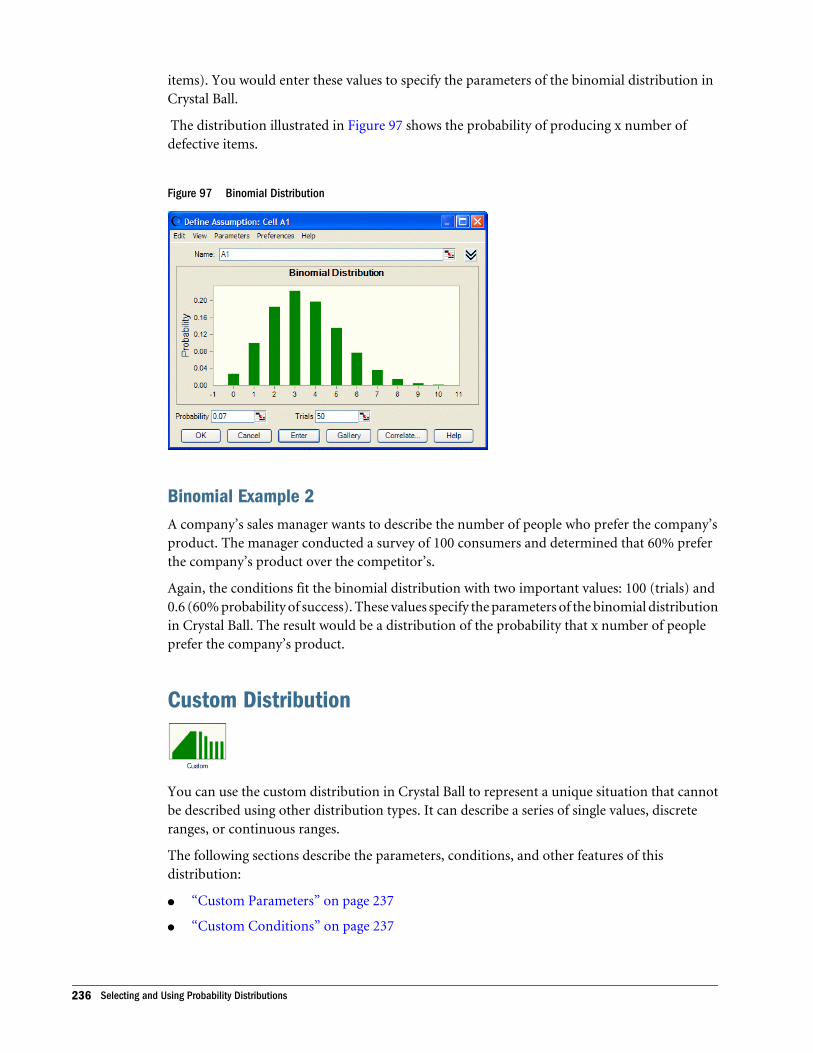
items). You would enter these values to specify the parameters of the binomial distribution inCrystal Ball.
The distribution illustrated in Figure 97 shows the probability of producing x number ofdefective items.
Figure 97 Binomial Distribution
Binomial Example 2A company’s sales manager wants to describe the number of people who prefer the company’sproduct. The manager conducted a survey of 100 consumers and determined that 60% preferthe company’s product over the competitor’s.
Again, the conditions fit the binomial distribution with two important values: 100 (trials) and0.6 (60% probability of success). These values specify the parameters of the binomial distributionin Crystal Ball. The result would be a distribution of the probability that x number of peopleprefer the company’s product.
Custom Distribution
You can use the custom distribution in Crystal Ball to represent a unique situation that cannotbe described using other distribution types. It can describe a series of single values, discreteranges, or continuous ranges.
The following sections describe the parameters, conditions, and other features of thisdistribution:
l “Custom Parameters” on page 237
l “Custom Conditions” on page 237
236 Selecting and Using Probability Distributions
Also see “ Using the Custom Distribution” on page 265.
Custom ParametersVariable, see “ Using the Custom Distribution” on page 265.
Custom ConditionsThe custom distribution is used under these conditions:
l It is a flexible distribution, used to represent a situation you cannot describe with otherdistribution types.
l It can be continuous, discrete, or a combination of both and can be used to input an entireset of data points from a range of cells.
For an example of a custom distribution, see the ClearView tutorial (“Growth Rate Assumption:Custom Distribution” on page 339). Also see “ Using the Custom Distribution” on page 265.
Discrete Uniform Distribution
In the discrete uniform distribution, you know the minimum and maximum values and youknow that all non-continuous values between the minimum and maximum are equally likely tooccur. It can be used to describe a real estate appraisal or a leak in a pipe. It is the discreteequivalent of the continuous uniform distribution (“Uniform Distribution” on page 261).
The following sections describe the parameters, conditions, and other features of thisdistribution:
l “Discrete Uniform Parameters” on page 237
l “Discrete Uniform Conditions” on page 237
l “Discrete Uniform Example” on page 238
Discrete Uniform ParametersMinimum, Maximum
Discrete Uniform ConditionsThe discrete uniform distribution is used under these conditions:
l Minimum is fixed.
l Maximum is fixed.
l All values in range are equally likely to occur.
Probability Distribution Descriptions 237
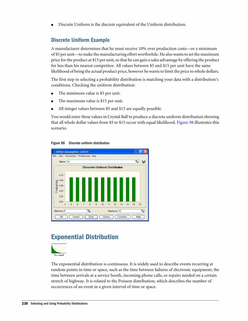
l Discrete Uniform is the discrete equivalent of the Uniform distribution.
Discrete Uniform ExampleA manufacturer determines that he must receive 10% over production costs—or a minimumof $5 per unit—to make the manufacturing effort worthwhile. He also wants to set the maximumprice for the product at $15 per unit, so that he can gain a sales advantage by offering the productfor less than his nearest competitor. All values between $5 and $15 per unit have the samelikelihood of being the actual product price, however he wants to limit the price to whole dollars.
The first step in selecting a probability distribution is matching your data with a distribution’sconditions. Checking the uniform distribution:
l The minimum value is $5 per unit.
l The maximum value is $15 per unit.
l All integer values between $5 and $15 are equally possible.
You would enter these values in Crystal Ball to produce a discrete uniform distribution showingthat all whole dollar values from $5 to $15 occur with equal likelihood. Figure 98 illustrates thisscenario.
Figure 98 Discrete uniform distribution
Exponential Distribution
The exponential distribution is continuous. It is widely used to describe events recurring atrandom points in time or space, such as the time between failures of electronic equipment, thetime between arrivals at a service booth, incoming phone calls, or repairs needed on a certainstretch of highway. It is related to the Poisson distribution, which describes the number ofoccurrences of an event in a given interval of time or space.
238 Selecting and Using Probability Distributions

The following sections describe the parameters, conditions, and other features of thisdistribution:
l “Exponential Parameter” on page 239
l “Exponential Conditions” on page 239
l “Exponential Example 1” on page 239
l “Exponential Example 2” on page 240
Exponential ParameterRate
Exponential ConditionsThe exponential distribution is used under these conditions:
l Distribution describes the time between occurrences.
l Distribution is not affected by previous events.
Exponential Example 1A travel agency wants to describe the time between incoming telephone calls when the calls areaveraging about 35 every 10 minutes. This same example was used for the Poisson distributionto describe the number of calls arriving every 10 minutes.
The first step in selecting a probability distribution is matching your data with a distribution’sconditions. Checking the exponential distribution:
l The travel agency wants to describe the time between successive telephone calls.
l The phone calls are not affected by previous history. The probability of receiving 35 callsevery 10 minutes remains the same.
The conditions in this example match those of the exponential distribution.
The exponential distribution has only one parameter: rate. The conditions outlined in thisexample include the value for this parameter: 35 (calls) every 10 minutes or a rate of 35. Enterthis value to set the parameter of the exponential distribution in Crystal Ball.
The distribution in Figure 99 shows the probability that x number of time units (10 minutes inthis case) will pass between calls.
Probability Distribution Descriptions 239
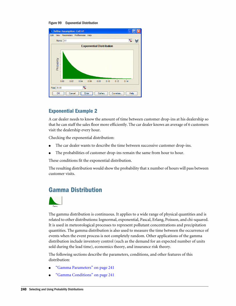
Figure 99 Exponential Distribution
Exponential Example 2A car dealer needs to know the amount of time between customer drop-ins at his dealership sothat he can staff the sales floor more efficiently. The car dealer knows an average of 6 customersvisit the dealership every hour.
Checking the exponential distribution:
l The car dealer wants to describe the time between successive customer drop-ins.
l The probabilities of customer drop-ins remain the same from hour to hour.
These conditions fit the exponential distribution.
The resulting distribution would show the probability that x number of hours will pass betweencustomer visits.
Gamma Distribution
The gamma distribution is continuous. It applies to a wide range of physical quantities and isrelated to other distributions: lognormal, exponential, Pascal, Erlang, Poisson, and chi-squared.It is used in meteorological processes to represent pollutant concentrations and precipitationquantities. The gamma distribution is also used to measure the time between the occurrence ofevents when the event process is not completely random. Other applications of the gammadistribution include inventory control (such as the demand for an expected number of unitssold during the lead time), economics theory, and insurance risk theory.
The following sections describe the parameters, conditions, and other features of thisdistribution:
l “Gamma Parameters” on page 241
l “Gamma Conditions” on page 241
240 Selecting and Using Probability Distributions
l “Gamma Example 1” on page 241
l “Gamma Example 2” on page 242
l “Chi-square and Erlang Distributions” on page 242
Gamma ParametersLocation, Scale, Shape
Gamma Conditionsl Possible occurrences in any unit of measurement are not limited.
l Occurrences are independent.
l Average numbers of occurrences are constant from unit to unit.
Gamma Example 1A computer dealership knows that the lead time for re-ordering their most popular computersystem is 4 weeks. Based upon an average demand of 1 unit per day, the dealership wants tomodel the number of business days it will take to sell 20 systems.
Checking the conditions of the gamma distribution:
l The number of possible customers demanding to buy the computer system is unlimited.
l The decisions of customers to buy the system are independent.
l The demand remains constant from week to week.
These conditions match those of the gamma distribution. (Note that in this example thedealership has made several simplifying assumptions about the conditions. In reality, the totalnumber of computer purchasers is finite, and some might have influenced the purchasingdecisions of others.)
The shape parameter is used to specify the r th occurrence of the Poisson event. In this example,you would enter 20 for the shape parameter (5 units per week times 4 weeks). The result is adistribution showing the probability that x number of business days will pass until the 20thsystem is sold.
Figure 100 illustrates the gamma distribution.
Probability Distribution Descriptions 241
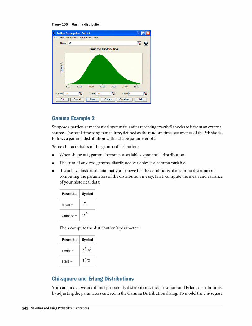
Figure 100 Gamma distribution
Gamma Example 2Suppose a particular mechanical system fails after receiving exactly 5 shocks to it from an externalsource. The total time to system failure, defined as the random time occurrence of the 5th shock,follows a gamma distribution with a shape parameter of 5.
Some characteristics of the gamma distribution:
l When shape = 1, gamma becomes a scalable exponential distribution.
l The sum of any two gamma-distributed variables is a gamma variable.
l If you have historical data that you believe fits the conditions of a gamma distribution,computing the parameters of the distribution is easy. First, compute the mean and varianceof your historical data:
Parameter Symbol
mean =
variance =
Then compute the distribution’s parameters:
Parameter Symbol
shape =
scale =
Chi-square and Erlang DistributionsYou can model two additional probability distributions, the chi-square and Erlang distributions,by adjusting the parameters entered in the Gamma Distribution dialog. To model the chi-square
242 Selecting and Using Probability Distributions
distributions with parameters N and S, where N = number of degrees of freedom and S = scale,set the parameters as follows:
Parameter Symbol
shape =
scale =
The chi-square distribution is the sum of the squares of N normal variates.
The Erlang distribution is identical to the gamma distribution, except the shape parameter isrestricted to integer values. Mathematically, the Erlang distribution is a summation of Nexponential distributions.
Geometric Distribution
The geometric distribution is discrete. It describes the number of trials until the first successfuloccurrence, such as the number of times you need to spin a roulette wheel before you win orhow many wells to dril before you strike oil.
The following sections describe the parameters, conditions, and other features of thisdistribution:
l “Geometric Parameter” on page 243
l “Geometric Conditions” on page 243
l “Geometric Example 1” on page 244
l “Geometric Example 2” on page 244
Geometric ParameterProbability
Geometric ConditionsThe geometric distribution is used under these conditions:
l Number of trials is not fixed.
l Trials continue until the first success.
l Probability of success is the same from trial to trial; if there is a 10% probability, this isentered 0.10.
Probability Distribution Descriptions 243
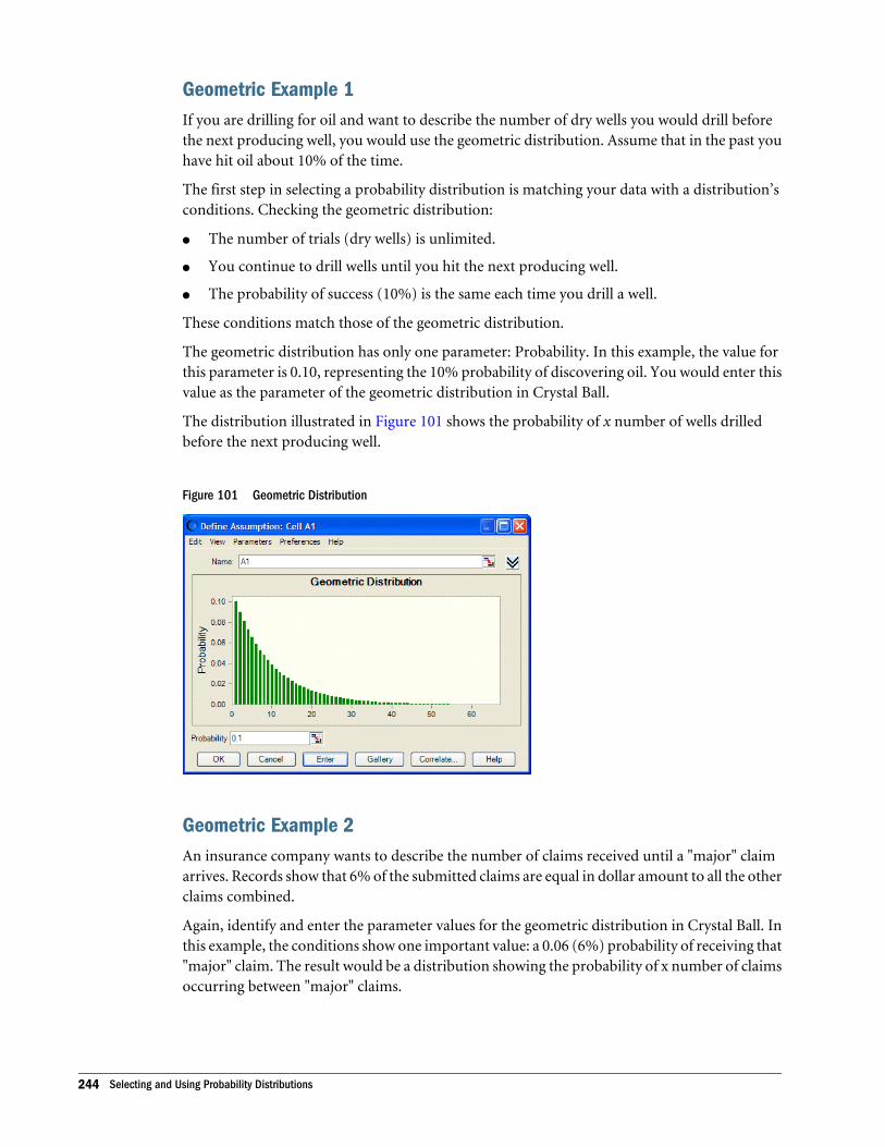
Geometric Example 1If you are drilling for oil and want to describe the number of dry wells you would drill beforethe next producing well, you would use the geometric distribution. Assume that in the past youhave hit oil about 10% of the time.
The first step in selecting a probability distribution is matching your data with a distribution’sconditions. Checking the geometric distribution:
l The number of trials (dry wells) is unlimited.
l You continue to drill wells until you hit the next producing well.
l The probability of success (10%) is the same each time you drill a well.
These conditions match those of the geometric distribution.
The geometric distribution has only one parameter: Probability. In this example, the value forthis parameter is 0.10, representing the 10% probability of discovering oil. You would enter thisvalue as the parameter of the geometric distribution in Crystal Ball.
The distribution illustrated in Figure 101 shows the probability of x number of wells drilledbefore the next producing well.
Figure 101 Geometric Distribution
Geometric Example 2An insurance company wants to describe the number of claims received until a "major" claimarrives. Records show that 6% of the submitted claims are equal in dollar amount to all the otherclaims combined.
Again, identify and enter the parameter values for the geometric distribution in Crystal Ball. Inthis example, the conditions show one important value: a 0.06 (6%) probability of receiving that"major" claim. The result would be a distribution showing the probability of x number of claimsoccurring between "major" claims.
244 Selecting and Using Probability Distributions
Hypergeometric Distribution
The hypergeometric distribution is discrete. It is similar to the binomial distribution. Bothdescribe the number of times a particular event occurs in a fixed number of trials. However,binomial distribution trials are independent, while hypergeometric distribution trials changethe success rate for each subsequent trial and are called "trials without replacement." Thehypergeometric distribution can be used for sampling problems such as the chance of pickinga defective part from a box (without returning parts to the box for the next trial).
The following sections describe the parameters, conditions, and other features of thisdistribution:
l “Hypergeometric Parameters” on page 245
l “Hypergeometric Conditions” on page 245
l “Hypergeometric Example 1” on page 245
l “Hypergeometric Example 2” on page 246
Hypergeometric ParametersSuccess, Trials, Population
Hypergeometric ConditionsThe hypergeometric distribution is used under these conditions:
l Total number of items (population) is fixed.
l Sample size (number of trials) is a portion of the population.
l Probability of success changes after each trial.
Hypergeometric Example 1You want to describe the number of consumers in a fixed population who prefer Brand X. Youare dealing with a total population of 40 consumers, of which 30 prefer Brand X and 10 preferBrand Y. You survey 20 of those consumers.
The first step in selecting a probability distribution is matching your data with a distribution’sconditions. Checking the hypergeometric distribution:
l The population size (40) is fixed.
l The sample size (20 consumers) represents a portion of the population.
l Initially, 30 of 40 consumers preferred Brand X so the initial success rate is 30. This ratechanges each time you question one of the 20 consumers, depending on the preference ofthe previous consumer.
Probability Distribution Descriptions 245
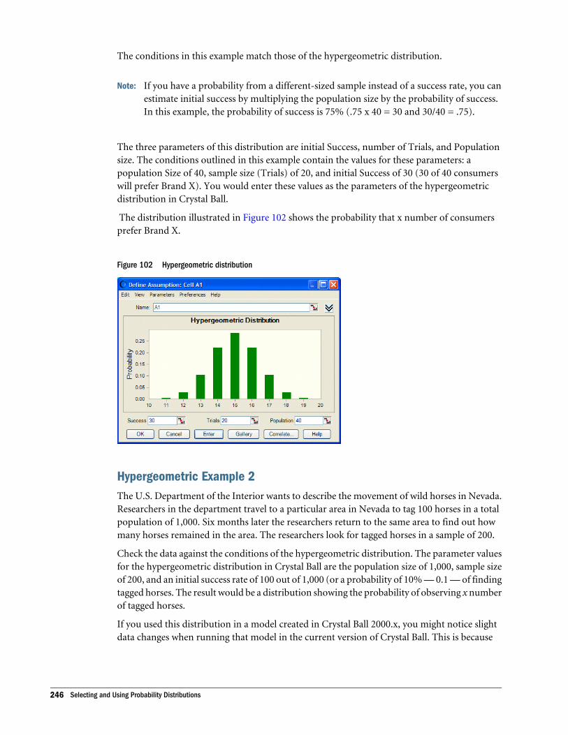
The conditions in this example match those of the hypergeometric distribution.
Note: If you have a probability from a different-sized sample instead of a success rate, you canestimate initial success by multiplying the population size by the probability of success.In this example, the probability of success is 75% (.75 x 40 = 30 and 30/40 = .75).
The three parameters of this distribution are initial Success, number of Trials, and Populationsize. The conditions outlined in this example contain the values for these parameters: apopulation Size of 40, sample size (Trials) of 20, and initial Success of 30 (30 of 40 consumerswill prefer Brand X). You would enter these values as the parameters of the hypergeometricdistribution in Crystal Ball.
The distribution illustrated in Figure 102 shows the probability that x number of consumersprefer Brand X.
Figure 102 Hypergeometric distribution
Hypergeometric Example 2The U.S. Department of the Interior wants to describe the movement of wild horses in Nevada.Researchers in the department travel to a particular area in Nevada to tag 100 horses in a totalpopulation of 1,000. Six months later the researchers return to the same area to find out howmany horses remained in the area. The researchers look for tagged horses in a sample of 200.
Check the data against the conditions of the hypergeometric distribution. The parameter valuesfor the hypergeometric distribution in Crystal Ball are the population size of 1,000, sample sizeof 200, and an initial success rate of 100 out of 1,000 (or a probability of 10% — 0.1 — of findingtagged horses. The result would be a distribution showing the probability of observing x numberof tagged horses.
If you used this distribution in a model created in Crystal Ball 2000.x, you might notice slightdata changes when running that model in the current version of Crystal Ball. This is because
246 Selecting and Using Probability Distributions
some rounding might occur when converting the probability parameter used in previous releasesto the success parameter used in this version of Crystal Ball.
Logistic Distribution
The logistic distribution is continuous. It is commonly used to describe growth (the size of apopulation expressed as a function of a time variable). It can also be used to describe chemicalreactions and the course of growth for a population or individual.
The following sections describe the parameters, conditions, and other features of thisdistribution:
l “Logistic Parameters” on page 247
l “Logistic Conditions” on page 247
l “Calculating Logistic Parameters” on page 247
Logistic ParametersMean, Scale
Logistic ConditionsThe logistic distribution is used under these conditions:
l Conditions and parameters are complex. See: Fishman, G. Springer Series in OperationsResearch. NY: Springer-Verlag, 1996.
Note: The mean parameter is the average value, which for this distribution is the same asthe mode, since this is a symmetrical distribution. After you select the meanparameter, you can estimate the scale parameter. The scale parameter is a numbergreater than 0. The larger the scale parameter, the greater the variance.
Calculating Logistic ParametersThere are two standard parameters for the logistic distribution: mean and scale. The meanparameter is the average value, which for this distribution is the same as the mode, since this isa symmetrical distribution.
After you select the mean parameter, you can estimate the scale parameter. The scale parameteris a number greater than 0. The larger the scale parameter, the greater the variance. The scaleparameter’s symbol is:
To calculate a more exact scale, you can estimate the variance and use the equation:
Probability Distribution Descriptions 247
Lognormal Distribution
The lognormal distribution is continuous. It is widely used in situations where values arepositively skewed, for example, for determining stock prices, real estate prices, pay scales, andoil reservoir size.
The following sections describe the parameters, conditions, and other features of thisdistribution:
l “Lognormal Parameters” on page 248
l “Lognormal Conditions” on page 248
l “Lognormal Example” on page 248
l “Lognormal Parameter Sets” on page 249
Lognormal ParametersLocation, Mean, Standard Deviation
Lognormal ConditionsThe lognormal distribution is used under these conditions:
l Upper and lower limits are unlimited, but the uncertain variable cannot fall below the valueof the location parameter.
l Distribution is positively skewed, with most values near lower limit.
l Natural logarithm of the distribution is a normal distribution.
Lognormal ExampleThe lognormal distribution can be used to model the price of a particular stock. You purchasea stock today at $50. You expect that the stock will be worth $70 at the end of the year. If thestock price drops at the end of the year, rather than appreciating, you know that the lowest valueit can drop to is $0.
On the other hand, the stock could end up with a price much higher than expected, thus implyingno upper limit on the rate of return. In summary, your losses are limited to your originalinvestment, but your gains are unlimited.
Using historical data, you can determine that the standard deviation of the stock’s price is $12.
248 Selecting and Using Probability Distributions
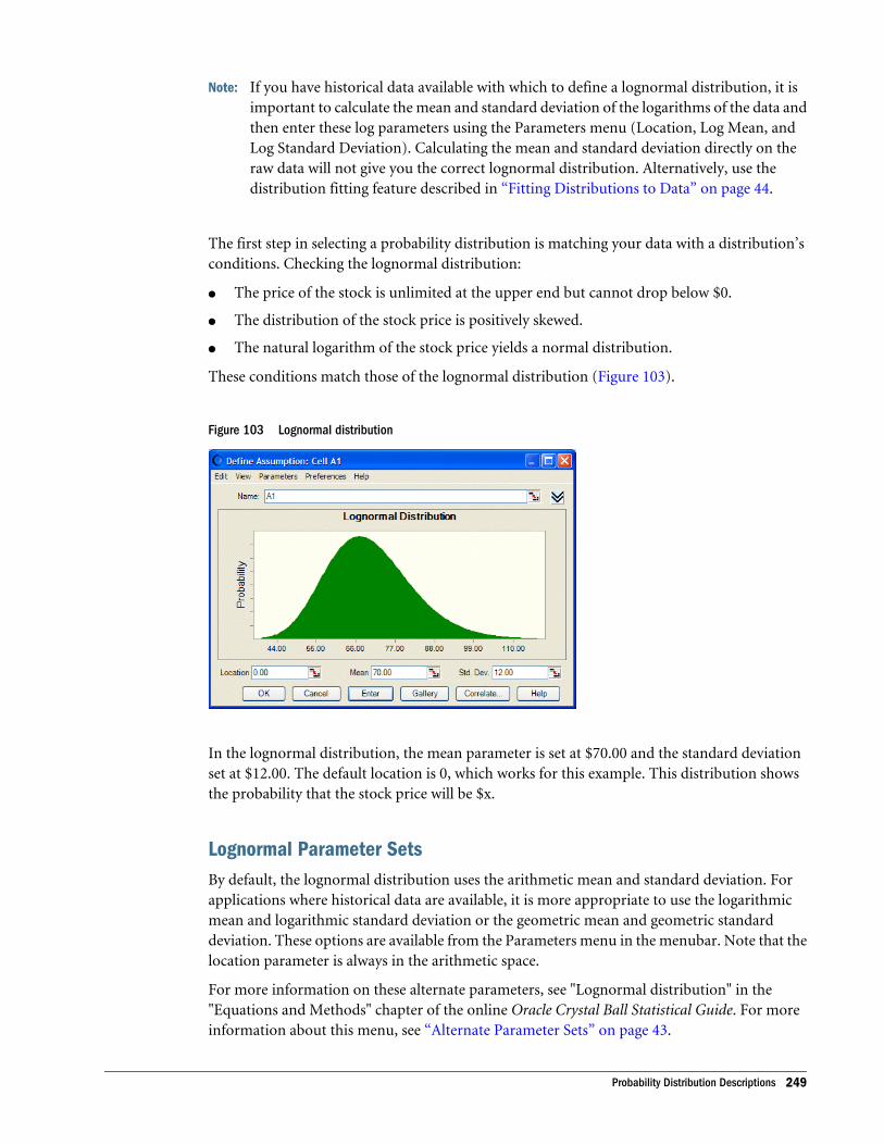
Note: If you have historical data available with which to define a lognormal distribution, it isimportant to calculate the mean and standard deviation of the logarithms of the data andthen enter these log parameters using the Parameters menu (Location, Log Mean, andLog Standard Deviation). Calculating the mean and standard deviation directly on theraw data will not give you the correct lognormal distribution. Alternatively, use thedistribution fitting feature described in “Fitting Distributions to Data” on page 44.
The first step in selecting a probability distribution is matching your data with a distribution’sconditions. Checking the lognormal distribution:
l The price of the stock is unlimited at the upper end but cannot drop below $0.
l The distribution of the stock price is positively skewed.
l The natural logarithm of the stock price yields a normal distribution.
These conditions match those of the lognormal distribution (Figure 103).
Figure 103 Lognormal distribution
In the lognormal distribution, the mean parameter is set at $70.00 and the standard deviationset at $12.00. The default location is 0, which works for this example. This distribution showsthe probability that the stock price will be $x.
Lognormal Parameter SetsBy default, the lognormal distribution uses the arithmetic mean and standard deviation. Forapplications where historical data are available, it is more appropriate to use the logarithmicmean and logarithmic standard deviation or the geometric mean and geometric standarddeviation. These options are available from the Parameters menu in the menubar. Note that thelocation parameter is always in the arithmetic space.
For more information on these alternate parameters, see "Lognormal distribution" in the"Equations and Methods" chapter of the online Oracle Crystal Ball Statistical Guide. For moreinformation about this menu, see “Alternate Parameter Sets” on page 43.
Probability Distribution Descriptions 249
Maximum Extreme Distribution
The maximum extreme distribution is continuous. It is commonly used to describe the largestvalue of a response over a period of time: for example, in flood flows, rainfall, and earthquakes.Other applications include the breaking strengths of materials, construction design, and aircraftloads and tolerances. This distribution is also known as the Gumbel distribution. and is closelyrelated to the minimum extreme distribution, its "mirror image."
The following sections describe the parameters, conditions, and other features of thisdistribution:
l “Maximum Extreme Parameters” on page 250
l “Maximum Extreme Conditions” on page 250
l “Calculating Maximum Extreme Parameters” on page 250
Maximum Extreme ParametersLikeliest, Scale
Maximum Extreme ConditionsThe maximum extreme distribution is used under these conditions:
l Conditions and parameters are complex. See: Castillo, Enrique. Extreme Value Theory inEngineering. London: Academic Press, 1988.
Note: After you select the Likeliest parameter, you can estimate the Scale parameter. TheScale parameter is a number greater than 0. The larger the Scale parameter, the greaterthe variance.
Calculating Maximum Extreme ParametersThere are two standard parameters for the maximum extreme value distribution: Likeliest andScale. The Likeliest parameter is the most likely value for the variable (the highest point on theprobability distribution, or mode).
After you select the Likeliest parameter, you can estimate the Scale parameter. The Scaleparameter is a number greater than 0. The larger the Scale parameter, the greater the variance.
The Scale parameter symbol is:
To calculate a more exact scale, you can estimate the mean and use the equation:
250 Selecting and Using Probability Distributions
Or estimate the variance and use the equation:
Minimum Extreme Distribution
The minimum extreme distribution is continuous. It is commonly used to describe the smallestvalue of a response over a period of time: for example, rainfall during a drought. This distributionis closely related to the maximum extreme distribution.
The following sections describe the parameters, conditions, and other features of thisdistribution:
l “Minimum Extreme Parameters” on page 251
l “Minimum Extreme Conditions” on page 251
l “Calculating Minimum Extreme Parameters” on page 251
Minimum Extreme ParametersLikeliest, Scale
Minimum Extreme ConditionsThe minimum extreme distribution is used under these conditions:
l Conditions and parameters are complex. See: Castillo, Enrique. Extreme Value Theory inEngineering. London: Academic Press, 1988.
Note: After you select the Likeliest parameter, you can estimate the Scale parameter. TheScale parameter is a number greater than 0. The larger the Scale parameter, the greaterthe variance.
Calculating Minimum Extreme ParametersThere are two standard parameters for the minimum extreme value distribution: Likeliest andScale. The Likeliest parameter is the most likely value for the variable (the highest point on theprobability distribution, or mode).
After you select the Likeliest parameter, you can estimate the Scale parameter. The Scaleparameter is a number greater than 0. The larger the Scale parameter, the greater the variance.
The Scale parameter symbol is:
Probability Distribution Descriptions 251
To calculate a more exact scale, you can estimate the mean and use the equation:
Or estimate the variance and use the equation:
Negative Binomial Distribution
The negative binomial distribution is discrete. It is useful for modeling the distribution of thenumber of trials until the rth successful occurrence, such as the number of sales calls you needto make to close ten orders. It is essentially a super-distribution of the geometric distribution.
The following sections describe the parameters, conditions, and other features of thisdistribution:
l “Negative Binomial Parameters” on page 252
l “Negative Binomial Conditions” on page 252
l “Negative Binomial Example” on page 252
Negative Binomial ParametersProbability, Shape
Negative Binomial ConditionsThe negative binomial distribution is used under these conditions:
l Number of trials is not fixed.
l Trials continue to the rth success (trials never less than r).
l Probability of success is the same from trial to trial.
Negative Binomial ExampleA manufacturer of jet engine turbines has an order to produce 50 turbines. Since about 20% ofthe turbines do not make it past the high-velocity spin test, the manufacturer will actually haveto produce more than 50 turbines.
Matching these conditions with the negative binomial distribution:
l The number of turbines to produce (trials) is not fixed.
252 Selecting and Using Probability Distributions
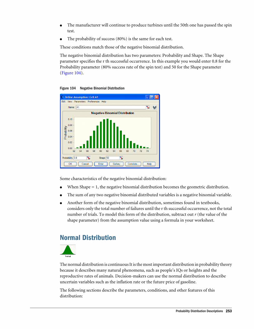
l The manufacturer will continue to produce turbines until the 50th one has passed the spintest.
l The probability of success (80%) is the same for each test.
These conditions match those of the negative binomial distribution.
The negative binomial distribution has two parameters: Probability and Shape. The Shapeparameter specifies the r th successful occurrence. In this example you would enter 0.8 for theProbability parameter (80% success rate of the spin test) and 50 for the Shape parameter(Figure 104).
Figure 104 Negative Binomial Distribution
Some characteristics of the negative binomial distribution:
l When Shape = 1, the negative binomial distribution becomes the geometric distribution.
l The sum of any two negative binomial distributed variables is a negative binomial variable.
l Another form of the negative binomial distribution, sometimes found in textbooks,considers only the total number of failures until the r th successful occurrence, not the totalnumber of trials. To model this form of the distribution, subtract out r (the value of theshape parameter) from the assumption value using a formula in your worksheet.
Normal Distribution
The normal distribution is continuous It is the most important distribution in probability theorybecause it describes many natural phenomena, such as people’s IQs or heights and thereproductive rates of animals. Decision-makers can use the normal distribution to describeuncertain variables such as the inflation rate or the future price of gasoline.
The following sections describe the parameters, conditions, and other features of thisdistribution:
Probability Distribution Descriptions 253
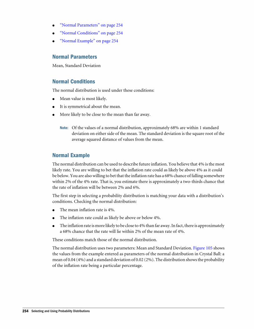
l “Normal Parameters” on page 254
l “Normal Conditions” on page 254
l “Normal Example” on page 254
Normal ParametersMean, Standard Deviation
Normal ConditionsThe normal distribution is used under these conditions:
l Mean value is most likely.
l It is symmetrical about the mean.
l More likely to be close to the mean than far away.
Note: Of the values of a normal distribution, approximately 68% are within 1 standarddeviation on either side of the mean. The standard deviation is the square root of theaverage squared distance of values from the mean.
Normal ExampleThe normal distribution can be used to describe future inflation. You believe that 4% is the mostlikely rate. You are willing to bet that the inflation rate could as likely be above 4% as it couldbe below. You are also willing to bet that the inflation rate has a 68% chance of falling somewherewithin 2% of the 4% rate. That is, you estimate there is approximately a two-thirds chance thatthe rate of inflation will be between 2% and 6%.
The first step in selecting a probability distribution is matching your data with a distribution’sconditions. Checking the normal distribution:
l The mean inflation rate is 4%.
l The inflation rate could as likely be above or below 4%.
l The inflation rate is more likely to be close to 4% than far away. In fact, there is approximatelya 68% chance that the rate will lie within 2% of the mean rate of 4%.
These conditions match those of the normal distribution.
The normal distribution uses two parameters: Mean and Standard Deviation. Figure 105 showsthe values from the example entered as parameters of the normal distribution in Crystal Ball: amean of 0.04 (4%) and a standard deviation of 0.02 (2%). The distribution shows the probabilityof the inflation rate being a particular percentage.
254 Selecting and Using Probability Distributions
Figure 105 Normal Distribution
Pareto Distribution
The Pareto distribution is continuous. It is widely used for the investigation of other distributionsassociated with such empirical phenomena as city population sizes, the occurrence of naturalresources, the size of companies, personal incomes, stock price fluctuations, and error clusteringin communication circuits.
The following sections describe the parameters, conditions, and other features of thisdistribution:
l “Pareto Parameters” on page 255
l “Pareto Conditions” on page 255
l “Calculating Pareto Parameters” on page 256
Pareto ParametersLocation, Shape
Pareto ConditionsThe Pareto distribution is used under these conditions:
l Conditions and parameters are complex. See: Fishman, G. Springer Series in OperationsResearch. NY: Springer-Verlag, 1996.
Note: Note: The location parameter is the lower bound for the variable. After you select theLocation parameter, you can estimate the shape parameter. The shape parameter is
Probability Distribution Descriptions 255
a number greater than 0, usually greater than 1. The larger the shape parameter, thesmaller the variance and the thicker the right tail of the distribution is displayed.
Calculating Pareto ParametersThere are two standard parameters for the Pareto distribution: Location and Shape. The Locationparameter is the lower bound for the variable.
After you select the Location parameter, you can estimate the Shape parameter. The Shapeparameter is a number greater than 0, usually greater than 1. The larger the Shape parameter,the smaller the variance and the thicker the right tail of the distribution is displayed.
The Shape parameter symbol is (beta).
The Location parameter symbol is L.
To calculate a more exact shape, you can estimate the mean and use the equation (for shapesgreater than 1):
Or estimate the variance and use the following equation (for shapes greater than 2):
Poisson Distribution
The Poisson distribution is discrete. It describes the number of times an event occurs in a giveninterval (usually time), such as the number of telephone calls per minute, the number of errorsper page in a document, or the number of defects per 100 yards of material.
The following sections describe the parameters, conditions, and other features of thisdistribution:
l “Poisson Parameter” on page 256
l “Poisson Conditions” on page 257
l “Poisson Example 1” on page 257
l “Poisson Example 2” on page 258
Poisson ParameterRate
256 Selecting and Using Probability Distributions
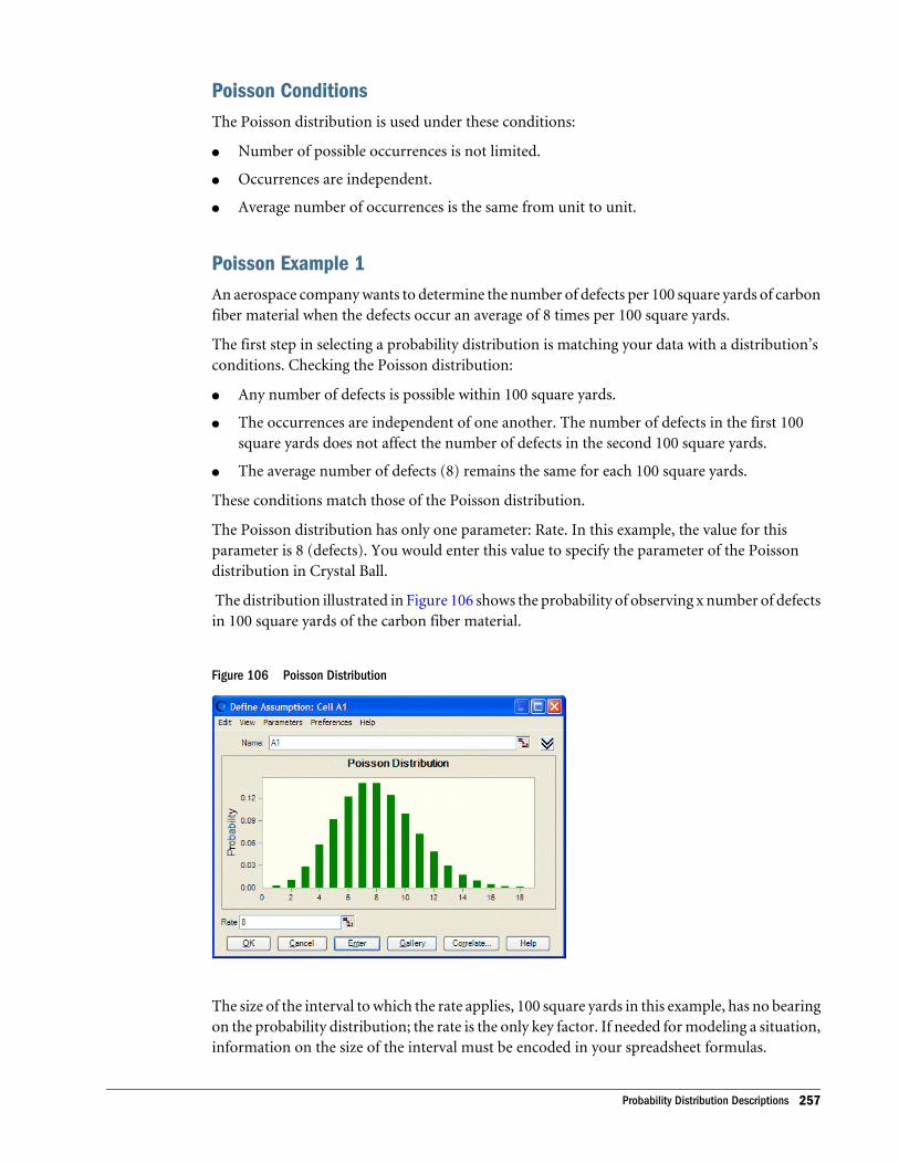
Poisson ConditionsThe Poisson distribution is used under these conditions:
l Number of possible occurrences is not limited.
l Occurrences are independent.
l Average number of occurrences is the same from unit to unit.
Poisson Example 1An aerospace company wants to determine the number of defects per 100 square yards of carbonfiber material when the defects occur an average of 8 times per 100 square yards.
The first step in selecting a probability distribution is matching your data with a distribution’sconditions. Checking the Poisson distribution:
l Any number of defects is possible within 100 square yards.
l The occurrences are independent of one another. The number of defects in the first 100square yards does not affect the number of defects in the second 100 square yards.
l The average number of defects (8) remains the same for each 100 square yards.
These conditions match those of the Poisson distribution.
The Poisson distribution has only one parameter: Rate. In this example, the value for thisparameter is 8 (defects). You would enter this value to specify the parameter of the Poissondistribution in Crystal Ball.
The distribution illustrated in Figure 106 shows the probability of observing x number of defectsin 100 square yards of the carbon fiber material.
Figure 106 Poisson Distribution
The size of the interval to which the rate applies, 100 square yards in this example, has no bearingon the probability distribution; the rate is the only key factor. If needed for modeling a situation,information on the size of the interval must be encoded in your spreadsheet formulas.
Probability Distribution Descriptions 257
Poisson Example 2A travel agency wants to describe the number of calls it receives in 10 minutes. The averagenumber of calls in 10 minutes is about 35.
Again, you begin by identifying and entering the values to set the parameters of the Poissondistribution in Crystal Ball. In this example, the conditions show one important value: 35 callsor a rate of 35. The result would be a distribution showing the probability of receiving x numberof calls in 10 minutes.
Student’s t Distribution
The Student’s t distribution is continuous. It is used to describe small sets of empirical data thatresemble a normal curve, but with thicker tails (more outliers). It is often used for econometricdata and exchange rates. For sets of data larger than 30, you can use the normal distributioninstead.
The following sections describe the parameters, conditions, and other features of thisdistribution:
l “Student’s t Parameters” on page 258
l “Student’s t Conditions” on page 258
l “Student’s t Example” on page 259
Student’s t ParametersMidpoint, Scale, Degrees of Freedom
Student’s t ConditionsThe Student’s t distribution is used under these conditions:
l Midpoint value is most likely.
l It is symmetrical about the mean.
l Approximates the Normal distribution when degrees of freedom are equal to or greater than30.
Note: Note: The Midpoint parameter is the central location of the distribution (also mode),the x-axis value where you want to place the peak of the distribution. The Degrees ofFreedom parameter controls the shape of the distribution. Smaller values result inthicker tails and less mass in the center. The Scale parameter affects the width of thedistribution by increasing the variance without affecting the overall shape andproportions of the curve. Scale can be used to widen the curve for easier reading and
258 Selecting and Using Probability Distributions
interpretation. For example, if the midpoint were a large number, say 5000, the scalecould be proportionately larger than if the midpoint were 500.
Student’s t ExampleFor examples, see “Normal Distribution” on page 253. The uses are the same except that thesample degrees of freedom will be < 30 for the Student’s t distribution.
Triangular Distribution
The triangular distribution is continuous. It describes a situation where you know the minimum,maximum, and most likely values to occur. It is useful with limited data in situations such assales estimates, the number of cars sold in a week, inventory numbers, and marketing costs. Forexample, you could describe the number of cars sold per week when past sales show theminimum, maximum, and usual number of cars sold.
The following sections describe the parameters, conditions, and other features of thisdistribution:
l “Triangular Parameters” on page 259
l “Triangular Conditions” on page 259
l “Triangular Example 1” on page 259
l “Triangular Example 2” on page 260
Triangular ParametersMinimum, Likeliest, Maximum
Triangular ConditionsThe triangular distribution is used under these conditions:
l Minimum and maximum are fixed.
l It has a most likely value in this range, which forms a triangle with the minimum andmaximum.
Triangular Example 1An owner needs to describe the amount of gasoline sold per week by his filling station. Past salesrecords show that a minimum of 3,000 gallons to a maximum of 7,000 gallons are sold per week,with most weeks showing sales of 5,000 gallons.
Probability Distribution Descriptions 259

The first step in selecting a probability distribution is matching your data with a distribution’sconditions. Checking the triangular distribution:
l The minimum number of gallons is 3,000.
l The maximum number of gallons is 7,000.
l The most likely number of gallons (5,000) falls between 3,000 and 7,000, forming a triangle.
These conditions match those of the triangular distribution.
The triangular distribution has three parameters: Minimum, Likeliest, and Maximum. Theconditions outlined in this example contain the values for these parameters: 3,000 (Minimum),5,000 (Likeliest), and 7,000 (Maximum). You would enter these values as the parameters of thetriangular distribution in Crystal Ball.
The following triangular distribution (Figure 107 on page 260shows the probability of x numberof gallons being sold per week.
Figure 107 Triangular Distribution
Triangular Example 2The triangular distribution also could be used to approximate a computer-controlled inventorysituation. The computer is programmed to keep an ideal supply of 25 items on the shelf, alwayskeep inventory at 10 items or more, and prevent inventory from ever rising above 30 items.
Check the triangular distribution conditions:
l The minimum inventory is 10 items.
l The maximum inventory is 30 items.
l The ideal level most frequently on the shelf is 25 items.
These conditions match those of the triangular distribution.
The result would be a distribution showing the probability of x number of items in inventory.
260 Selecting and Using Probability Distributions
Uniform Distribution
The uniform distribution is continuous. In the uniform distribution, you know the rangebetween the minimum and maximum values and you know that all values in the range are equallylikely to occur. It can be used to describe a real estate appraisal or a leak in a pipe.
The following sections describe the parameters, conditions, and other features of thisdistribution:
l “Uniform Parameters” on page 261
l “Uniform Conditions” on page 261
l “Uniform Example 1” on page 261
l “Uniform Example 2” on page 262
Uniform ParametersMinimum, Maximum
Uniform ConditionsThe uniform distribution is used under these conditions:
l Minimum is fixed.
l Maximum is fixed.
l All values in range are equally likely to occur.
l Discrete uniform is the discrete equivalent of the uniform distribution.
Uniform Example 1An investment company interested in purchasing a parcel of prime commercial real estate wantsto describe the appraised value of the property. The company expects an appraisal of at least$500,000 but not more than $900,000. They believe that all values between $500,000 and$900,000 have the same likelihood of being the actual appraised value.
The first step in selecting a probability distribution is matching your data with a distribution’sconditions. In this case:
l The minimum value is $500,000.
l The maximum value is $900,000.
l All values between $500,000 and $900,000 are equally possible.
These conditions match those of the uniform distribution. The uniform distribution has twoparameters: the Minimum ($500,000) and the Maximum ($900,000). You would enter thesevalues as the parameters of the uniform distribution in Crystal Ball (Figure 108).
Probability Distribution Descriptions 261
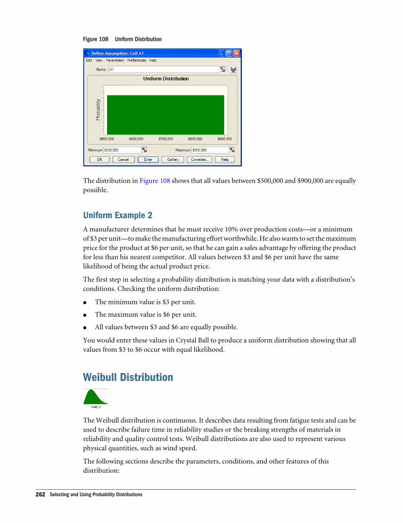
Figure 108 Uniform Distribution
The distribution in Figure 108 shows that all values between $500,000 and $900,000 are equallypossible.
Uniform Example 2A manufacturer determines that he must receive 10% over production costs—or a minimumof $3 per unit—to make the manufacturing effort worthwhile. He also wants to set the maximumprice for the product at $6 per unit, so that he can gain a sales advantage by offering the productfor less than his nearest competitor. All values between $3 and $6 per unit have the samelikelihood of being the actual product price.
The first step in selecting a probability distribution is matching your data with a distribution’sconditions. Checking the uniform distribution:
l The minimum value is $3 per unit.
l The maximum value is $6 per unit.
l All values between $3 and $6 are equally possible.
You would enter these values in Crystal Ball to produce a uniform distribution showing that allvalues from $3 to $6 occur with equal likelihood.
Weibull Distribution
The Weibull distribution is continuous. It describes data resulting from fatigue tests and can beused to describe failure time in reliability studies or the breaking strengths of materials inreliability and quality control tests. Weibull distributions are also used to represent variousphysical quantities, such as wind speed.
The following sections describe the parameters, conditions, and other features of thisdistribution:
262 Selecting and Using Probability Distributions
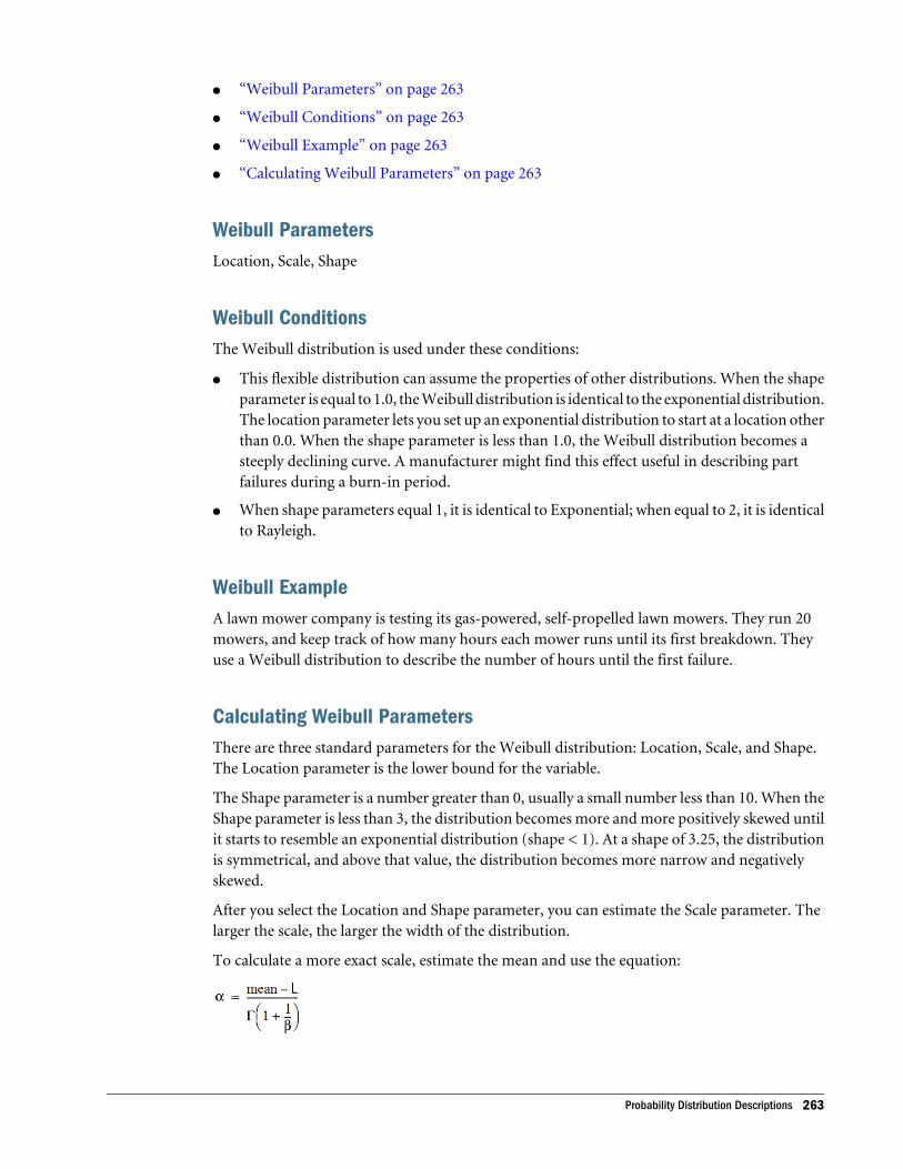
l “Weibull Parameters” on page 263
l “Weibull Conditions” on page 263
l “Weibull Example” on page 263
l “Calculating Weibull Parameters” on page 263
Weibull ParametersLocation, Scale, Shape
Weibull ConditionsThe Weibull distribution is used under these conditions:
l This flexible distribution can assume the properties of other distributions. When the shapeparameter is equal to 1.0, the Weibull distribution is identical to the exponential distribution.The location parameter lets you set up an exponential distribution to start at a location otherthan 0.0. When the shape parameter is less than 1.0, the Weibull distribution becomes asteeply declining curve. A manufacturer might find this effect useful in describing partfailures during a burn-in period.
l When shape parameters equal 1, it is identical to Exponential; when equal to 2, it is identicalto Rayleigh.
Weibull ExampleA lawn mower company is testing its gas-powered, self-propelled lawn mowers. They run 20mowers, and keep track of how many hours each mower runs until its first breakdown. Theyuse a Weibull distribution to describe the number of hours until the first failure.
Calculating Weibull ParametersThere are three standard parameters for the Weibull distribution: Location, Scale, and Shape.The Location parameter is the lower bound for the variable.
The Shape parameter is a number greater than 0, usually a small number less than 10. When theShape parameter is less than 3, the distribution becomes more and more positively skewed untilit starts to resemble an exponential distribution (shape < 1). At a shape of 3.25, the distributionis symmetrical, and above that value, the distribution becomes more narrow and negativelyskewed.
After you select the Location and Shape parameter, you can estimate the Scale parameter. Thelarger the scale, the larger the width of the distribution.
To calculate a more exact scale, estimate the mean and use the equation:
Probability Distribution Descriptions 263
where (alpha) is the scale, (beta) is the shape, L is the location, and (gamma) is the gammafunction. You can use the Excel GAMMALN function and Excel Solver to help you calculate thisparameter.
For this distribution, there is a 63% probability that x falls between a and a+L.
Or estimate the mode and use the equation:
where (alpha) is the scale, (beta) is the shape, and L is the location.
Yes-No Distribution
The yes-no distribution, also called the Bernoulli distribution, is a discrete distribution thatdescribes a set of observations that can have only one of two values, such as yes or no, successor failure, true or false, or heads or tails.
The following sections describe the parameters, conditions, and other features of thisdistribution:
l “Yes-No Parameters” on page 264
l “Yes-No Parameters” on page 264
l “Yes-No Example” on page 265
Yes-No ParametersProbability of Yes (1)
Yes-No ConditionsThe yes-no distribution is used under these conditions:
l For each trial, only 2 outcomes are possible, such as success or failure; the random variablecan have only one of two values, for example, 0 and 1.
l The mean is p, or probability (0 < p < 1).
l Trials are independent. Probability is the same from trial to trial.
l The Yes-No distribution is equivalent to the Binomial distribution with one trial.
264 Selecting and Using Probability Distributions
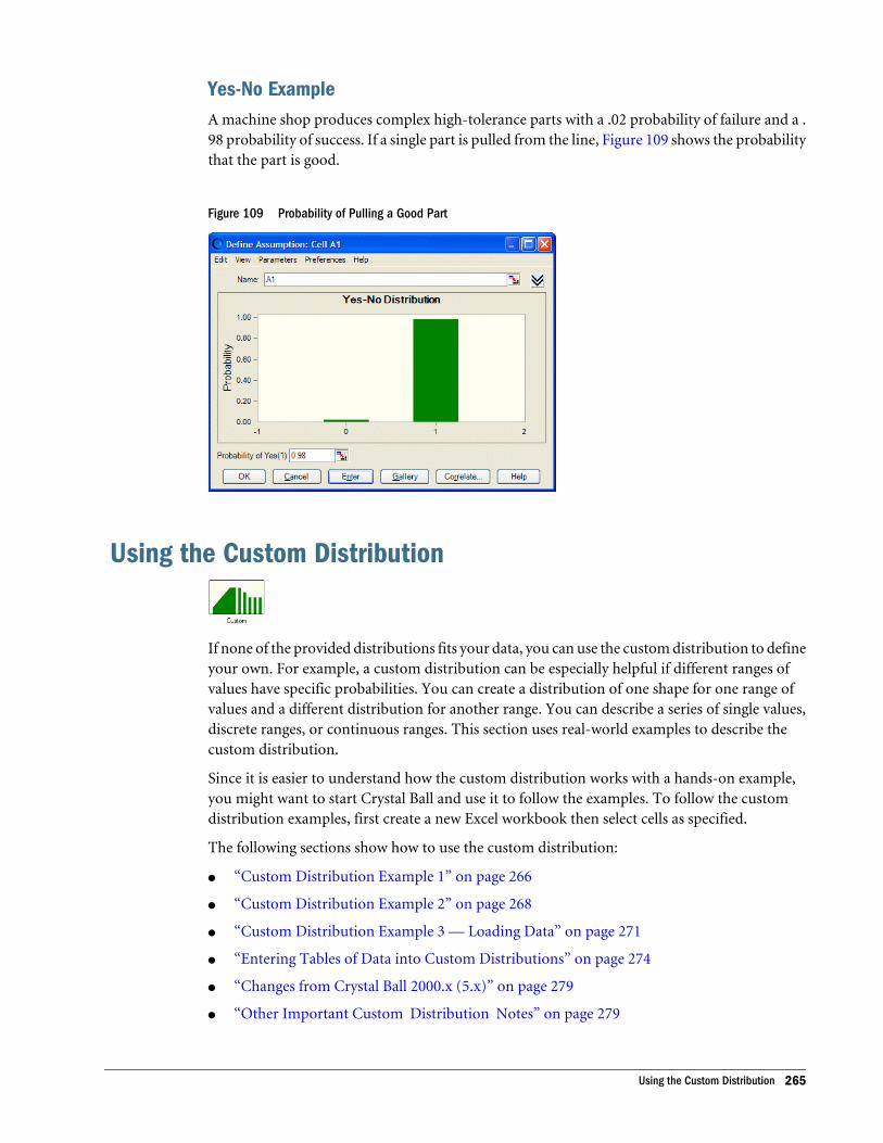
Yes-No ExampleA machine shop produces complex high-tolerance parts with a .02 probability of failure and a .98 probability of success. If a single part is pulled from the line, Figure 109 shows the probabilitythat the part is good.
Figure 109 Probability of Pulling a Good Part
Using the Custom Distribution
If none of the provided distributions fits your data, you can use the custom distribution to defineyour own. For example, a custom distribution can be especially helpful if different ranges ofvalues have specific probabilities. You can create a distribution of one shape for one range ofvalues and a different distribution for another range. You can describe a series of single values,discrete ranges, or continuous ranges. This section uses real-world examples to describe thecustom distribution.
Since it is easier to understand how the custom distribution works with a hands-on example,you might want to start Crystal Ball and use it to follow the examples. To follow the customdistribution examples, first create a new Excel workbook then select cells as specified.
The following sections show how to use the custom distribution:
l “Custom Distribution Example 1” on page 266
l “Custom Distribution Example 2” on page 268
l “Custom Distribution Example 3 — Loading Data” on page 271
l “Entering Tables of Data into Custom Distributions” on page 274
l “Changes from Crystal Ball 2000.x (5.x)” on page 279
l “Other Important Custom Distribution Notes” on page 279
Using the Custom Distribution 265
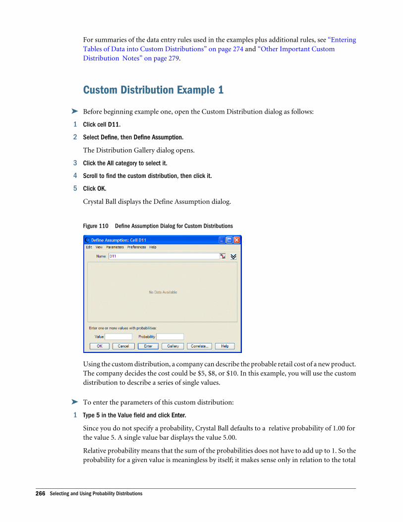
For summaries of the data entry rules used in the examples plus additional rules, see “EnteringTables of Data into Custom Distributions” on page 274 and “Other Important CustomDistribution Notes” on page 279.
Custom Distribution Example 1
ä Before beginning example one, open the Custom Distribution dialog as follows:
1 Click cell D11.
2 Select Define, then Define Assumption.
The Distribution Gallery dialog opens.
3 Click the All category to select it.
4 Scroll to find the custom distribution, then click it.
5 Click OK.
Crystal Ball displays the Define Assumption dialog.
Figure 110 Define Assumption Dialog for Custom Distributions
Using the custom distribution, a company can describe the probable retail cost of a new product.The company decides the cost could be $5, $8, or $10. In this example, you will use the customdistribution to describe a series of single values.
ä To enter the parameters of this custom distribution:
1 Type 5 in the Value field and click Enter.
Since you do not specify a probability, Crystal Ball defaults to a relative probability of 1.00 forthe value 5. A single value bar displays the value 5.00.
Relative probability means that the sum of the probabilities does not have to add up to 1. So theprobability for a given value is meaningless by itself; it makes sense only in relation to the total
266 Selecting and Using Probability Distributions
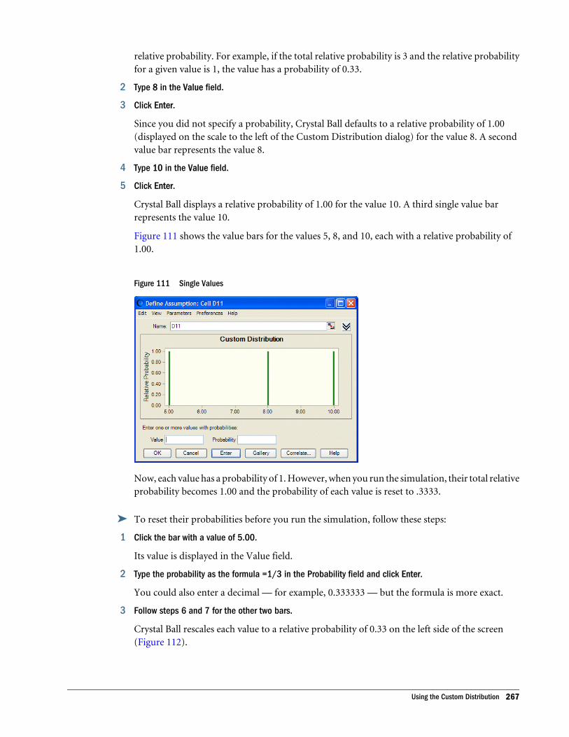
relative probability. For example, if the total relative probability is 3 and the relative probabilityfor a given value is 1, the value has a probability of 0.33.
2 Type 8 in the Value field.
3 Click Enter.
Since you did not specify a probability, Crystal Ball defaults to a relative probability of 1.00(displayed on the scale to the left of the Custom Distribution dialog) for the value 8. A secondvalue bar represents the value 8.
4 Type 10 in the Value field.
5 Click Enter.
Crystal Ball displays a relative probability of 1.00 for the value 10. A third single value barrepresents the value 10.
Figure 111 shows the value bars for the values 5, 8, and 10, each with a relative probability of1.00.
Figure 111 Single Values
Now, each value has a probability of 1. However, when you run the simulation, their total relativeprobability becomes 1.00 and the probability of each value is reset to .3333.
ä To reset their probabilities before you run the simulation, follow these steps:
1 Click the bar with a value of 5.00.
Its value is displayed in the Value field.
2 Type the probability as the formula =1/3 in the Probability field and click Enter.
You could also enter a decimal — for example, 0.333333 — but the formula is more exact.
3 Follow steps 6 and 7 for the other two bars.
Crystal Ball rescales each value to a relative probability of 0.33 on the left side of the screen(Figure 112).
Using the Custom Distribution 267
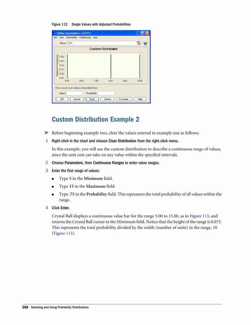
Figure 112 Single Values with Adjusted Probabilities
Custom Distribution Example 2
ä Before beginning example two, clear the values entered in example one as follows:
1 Right-click in the chart and choose Clear Distribution from the right-click menu.
In this example, you will use the custom distribution to describe a continuous range of values,since the unit cost can take on any value within the specified intervals.
2 Choose Parameters, then Continuous Ranges to enter value ranges.
3 Enter the first range of values:
l Type 5 in the Minimum field.
l Type 15 in the Maximum field.
l Type .75 in the Probability field. This represents the total probability of all values within therange.
4 Click Enter.
Crystal Ball displays a continuous value bar for the range 5.00 to 15.00, as in Figure 113, andreturns the Crystal Ball cursor to the Minimum field. Notice that the height of the range is 0.075.This represents the total probability divided by the width (number of units) in the range, 10(Figure 113).
268 Selecting and Using Probability Distributions
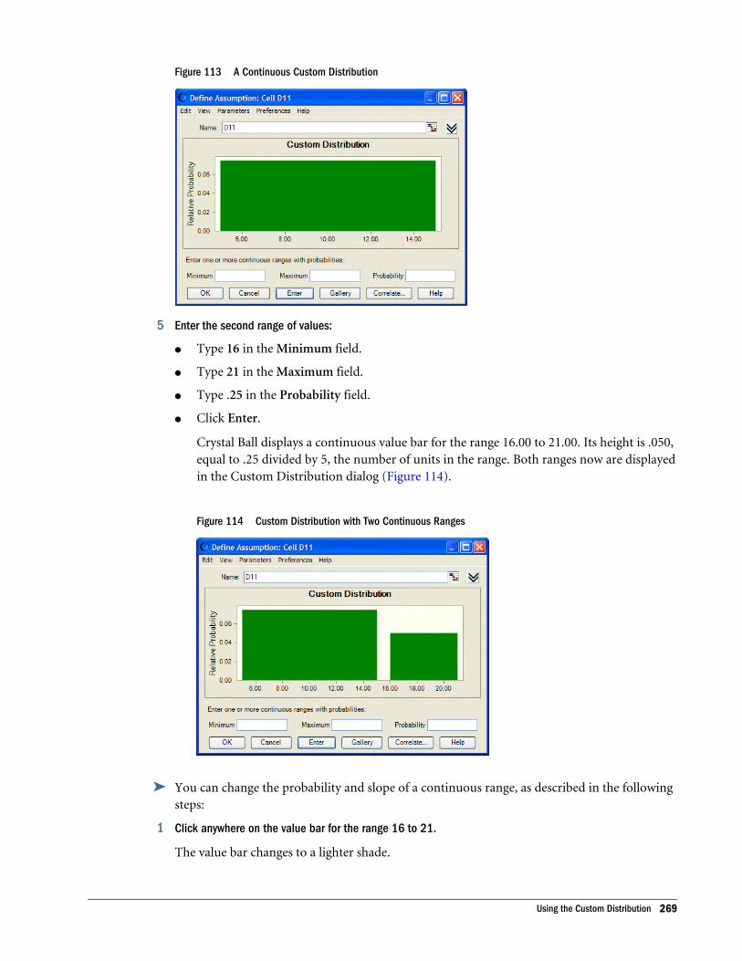
Figure 113 A Continuous Custom Distribution
5 Enter the second range of values:
l Type 16 in the Minimum field.
l Type 21 in the Maximum field.
l Type .25 in the Probability field.
l Click Enter.
Crystal Ball displays a continuous value bar for the range 16.00 to 21.00. Its height is .050,equal to .25 divided by 5, the number of units in the range. Both ranges now are displayedin the Custom Distribution dialog (Figure 114).
Figure 114 Custom Distribution with Two Continuous Ranges
ä You can change the probability and slope of a continuous range, as described in the followingsteps:
1 Click anywhere on the value bar for the range 16 to 21.
The value bar changes to a lighter shade.
Using the Custom Distribution 269
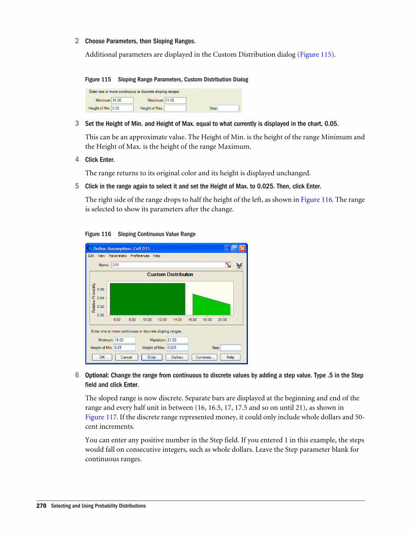
2 Choose Parameters, then Sloping Ranges.
Additional parameters are displayed in the Custom Distribution dialog (Figure 115).
Figure 115 Sloping Range Parameters, Custom Distribution Dialog
3 Set the Height of Min. and Height of Max. equal to what currently is displayed in the chart, 0.05.
This can be an approximate value. The Height of Min. is the height of the range Minimum andthe Height of Max. is the height of the range Maximum.
4 Click Enter.
The range returns to its original color and its height is displayed unchanged.
5 Click in the range again to select it and set the Height of Max. to 0.025. Then, click Enter.
The right side of the range drops to half the height of the left, as shown in Figure 116. The rangeis selected to show its parameters after the change.
Figure 116 Sloping Continuous Value Range
6 Optional: Change the range from continuous to discrete values by adding a step value. Type .5 in the Stepfield and click Enter.
The sloped range is now discrete. Separate bars are displayed at the beginning and end of therange and every half unit in between (16, 16.5, 17, 17.5 and so on until 21), as shown inFigure 117. If the discrete range represented money, it could only include whole dollars and 50-cent increments.
You can enter any positive number in the Step field. If you entered 1 in this example, the stepswould fall on consecutive integers, such as whole dollars. Leave the Step parameter blank forcontinuous ranges.
270 Selecting and Using Probability Distributions
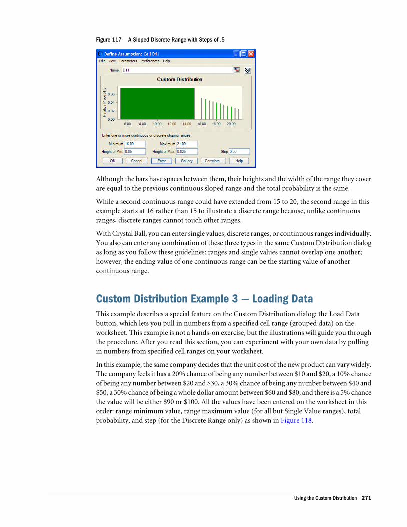
Figure 117 A Sloped Discrete Range with Steps of .5
Although the bars have spaces between them, their heights and the width of the range they coverare equal to the previous continuous sloped range and the total probability is the same.
While a second continuous range could have extended from 15 to 20, the second range in thisexample starts at 16 rather than 15 to illustrate a discrete range because, unlike continuousranges, discrete ranges cannot touch other ranges.
With Crystal Ball, you can enter single values, discrete ranges, or continuous ranges individually.You also can enter any combination of these three types in the same Custom Distribution dialogas long as you follow these guidelines: ranges and single values cannot overlap one another;however, the ending value of one continuous range can be the starting value of anothercontinuous range.
Custom Distribution Example 3 — Loading DataThis example describes a special feature on the Custom Distribution dialog: the Load Databutton, which lets you pull in numbers from a specified cell range (grouped data) on theworksheet. This example is not a hands-on exercise, but the illustrations will guide you throughthe procedure. After you read this section, you can experiment with your own data by pullingin numbers from specified cell ranges on your worksheet.
In this example, the same company decides that the unit cost of the new product can vary widely.The company feels it has a 20% chance of being any number between $10 and $20, a 10% chanceof being any number between $20 and $30, a 30% chance of being any number between $40 and$50, a 30% chance of being a whole dollar amount between $60 and $80, and there is a 5% chancethe value will be either $90 or $100. All the values have been entered on the worksheet in thisorder: range minimum value, range maximum value (for all but Single Value ranges), totalprobability, and step (for the Discrete Range only) as shown in Figure 118.
Using the Custom Distribution 271
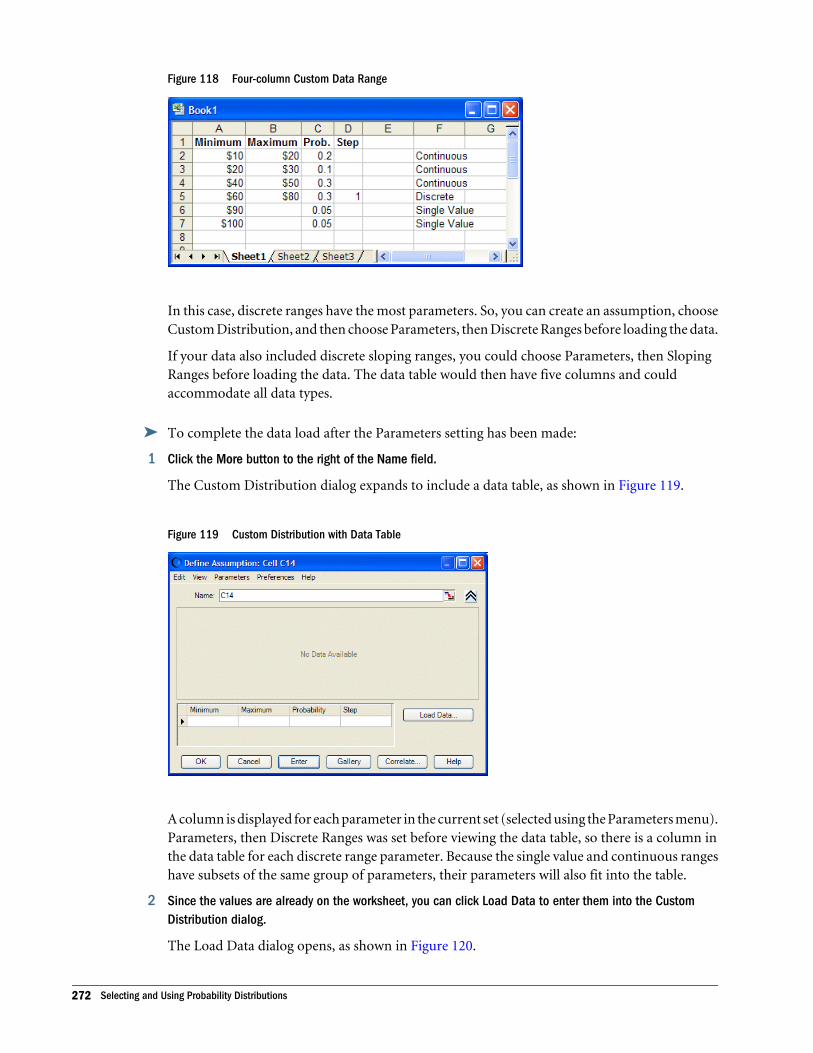
Figure 118 Four-column Custom Data Range
In this case, discrete ranges have the most parameters. So, you can create an assumption, chooseCustom Distribution, and then choose Parameters, then Discrete Ranges before loading the data.
If your data also included discrete sloping ranges, you could choose Parameters, then SlopingRanges before loading the data. The data table would then have five columns and couldaccommodate all data types.
ä To complete the data load after the Parameters setting has been made:
1 Click the More button to the right of the Name field.
The Custom Distribution dialog expands to include a data table, as shown in Figure 119.
Figure 119 Custom Distribution with Data Table
A column is displayed for each parameter in the current set (selected using the Parameters menu).Parameters, then Discrete Ranges was set before viewing the data table, so there is a column inthe data table for each discrete range parameter. Because the single value and continuous rangeshave subsets of the same group of parameters, their parameters will also fit into the table.
2 Since the values are already on the worksheet, you can click Load Data to enter them into the CustomDistribution dialog.
The Load Data dialog opens, as shown in Figure 120.
272 Selecting and Using Probability Distributions
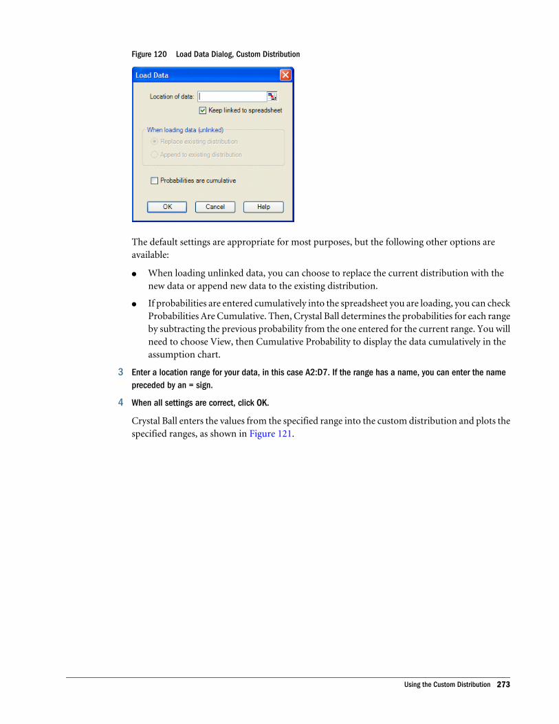
Figure 120 Load Data Dialog, Custom Distribution
The default settings are appropriate for most purposes, but the following other options areavailable:
l When loading unlinked data, you can choose to replace the current distribution with thenew data or append new data to the existing distribution.
l If probabilities are entered cumulatively into the spreadsheet you are loading, you can checkProbabilities Are Cumulative. Then, Crystal Ball determines the probabilities for each rangeby subtracting the previous probability from the one entered for the current range. You willneed to choose View, then Cumulative Probability to display the data cumulatively in theassumption chart.
3 Enter a location range for your data, in this case A2:D7. If the range has a name, you can enter the namepreceded by an = sign.
4 When all settings are correct, click OK.
Crystal Ball enters the values from the specified range into the custom distribution and plots thespecified ranges, as shown in Figure 121.
Using the Custom Distribution 273
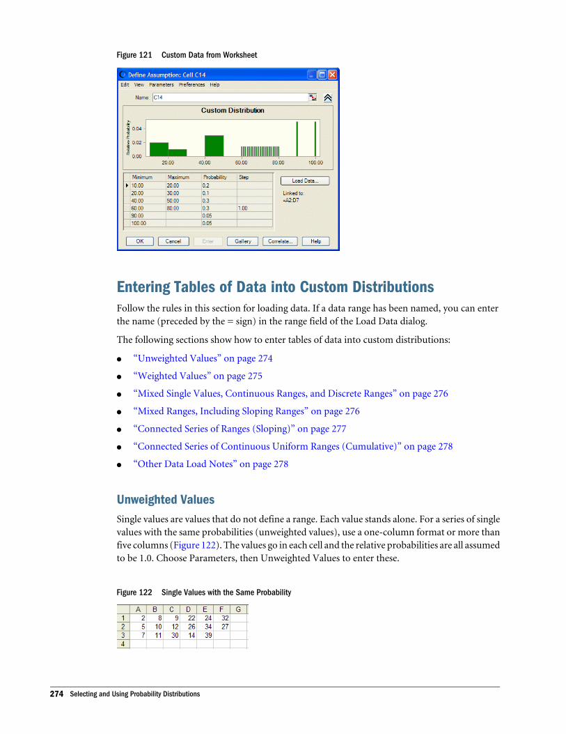
Figure 121 Custom Data from Worksheet
Entering Tables of Data into Custom DistributionsFollow the rules in this section for loading data. If a data range has been named, you can enterthe name (preceded by the = sign) in the range field of the Load Data dialog.
The following sections show how to enter tables of data into custom distributions:
l “Unweighted Values” on page 274
l “Weighted Values” on page 275
l “Mixed Single Values, Continuous Ranges, and Discrete Ranges” on page 276
l “Mixed Ranges, Including Sloping Ranges” on page 276
l “Connected Series of Ranges (Sloping)” on page 277
l “Connected Series of Continuous Uniform Ranges (Cumulative)” on page 278
l “Other Data Load Notes” on page 278
Unweighted ValuesSingle values are values that do not define a range. Each value stands alone. For a series of singlevalues with the same probabilities (unweighted values), use a one-column format or more thanfive columns (Figure 122). The values go in each cell and the relative probabilities are all assumedto be 1.0. Choose Parameters, then Unweighted Values to enter these.
Figure 122 Single Values with the Same Probability
274 Selecting and Using Probability Distributions
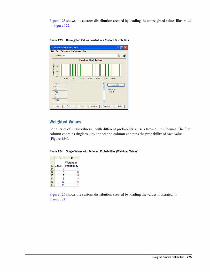
Figure 123 shows the custom distribution created by loading the unweighted values illustratedin Figure 122.
Figure 123 Unweighted Values Loaded in a Custom Distribution
Weighted ValuesFor a series of single values all with different probabilities, use a two-column format. The firstcolumn contains single values, the second column contains the probability of each value(Figure 124).
Figure 124 Single Values with Different Probabilities (Weighted Values)
Figure 125 shows the custom distribution created by loading the values illustrated inFigure 124.
Using the Custom Distribution 275
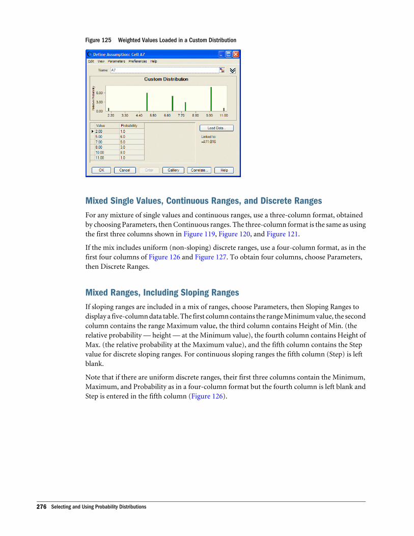
Figure 125 Weighted Values Loaded in a Custom Distribution
Mixed Single Values, Continuous Ranges, and Discrete RangesFor any mixture of single values and continuous ranges, use a three-column format, obtainedby choosing Parameters, then Continuous ranges. The three-column format is the same as usingthe first three columns shown in Figure 119, Figure 120, and Figure 121.
If the mix includes uniform (non-sloping) discrete ranges, use a four-column format, as in thefirst four columns of Figure 126 and Figure 127. To obtain four columns, choose Parameters,then Discrete Ranges.
Mixed Ranges, Including Sloping RangesIf sloping ranges are included in a mix of ranges, choose Parameters, then Sloping Ranges todisplay a five-column data table. The first column contains the range Minimum value, the secondcolumn contains the range Maximum value, the third column contains Height of Min. (therelative probability — height — at the Minimum value), the fourth column contains Height ofMax. (the relative probability at the Maximum value), and the fifth column contains the Stepvalue for discrete sloping ranges. For continuous sloping ranges the fifth column (Step) is leftblank.
Note that if there are uniform discrete ranges, their first three columns contain the Minimum,Maximum, and Probability as in a four-column format but the fourth column is left blank andStep is entered in the fifth column (Figure 126).
276 Selecting and Using Probability Distributions
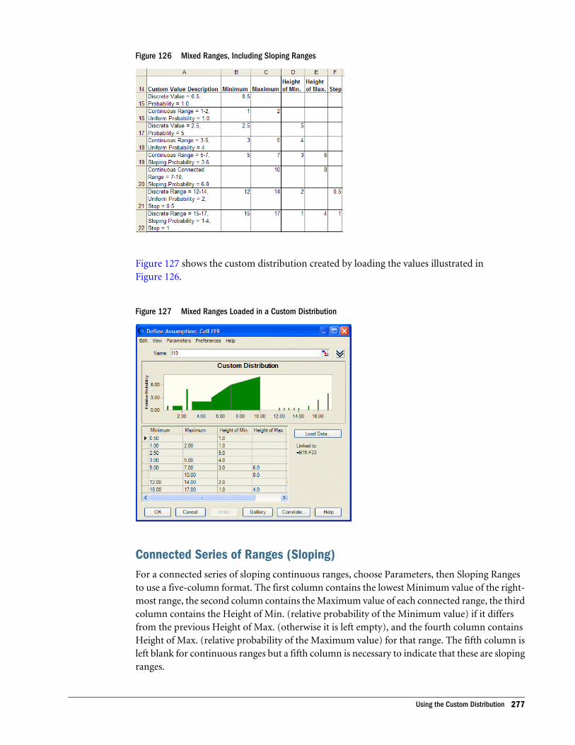
Figure 126 Mixed Ranges, Including Sloping Ranges
Figure 127 shows the custom distribution created by loading the values illustrated inFigure 126.
Figure 127 Mixed Ranges Loaded in a Custom Distribution
Connected Series of Ranges (Sloping)For a connected series of sloping continuous ranges, choose Parameters, then Sloping Rangesto use a five-column format. The first column contains the lowest Minimum value of the right-most range, the second column contains the Maximum value of each connected range, the thirdcolumn contains the Height of Min. (relative probability of the Minimum value) if it differsfrom the previous Height of Max. (otherwise it is left empty), and the fourth column containsHeight of Max. (relative probability of the Maximum value) for that range. The fifth column isleft blank for continuous ranges but a fifth column is necessary to indicate that these are slopingranges.
Using the Custom Distribution 277
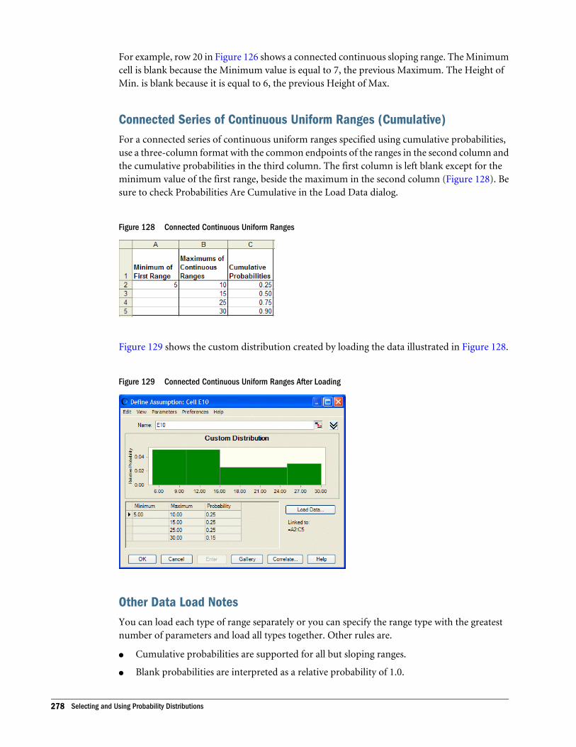
For example, row 20 in Figure 126 shows a connected continuous sloping range. The Minimumcell is blank because the Minimum value is equal to 7, the previous Maximum. The Height ofMin. is blank because it is equal to 6, the previous Height of Max.
Connected Series of Continuous Uniform Ranges (Cumulative)For a connected series of continuous uniform ranges specified using cumulative probabilities,use a three-column format with the common endpoints of the ranges in the second column andthe cumulative probabilities in the third column. The first column is left blank except for theminimum value of the first range, beside the maximum in the second column (Figure 128). Besure to check Probabilities Are Cumulative in the Load Data dialog.
Figure 128 Connected Continuous Uniform Ranges
Figure 129 shows the custom distribution created by loading the data illustrated in Figure 128.
Figure 129 Connected Continuous Uniform Ranges After Loading
Other Data Load NotesYou can load each type of range separately or you can specify the range type with the greatestnumber of parameters and load all types together. Other rules are.
l Cumulative probabilities are supported for all but sloping ranges.
l Blank probabilities are interpreted as a relative probability of 1.0.
278 Selecting and Using Probability Distributions
l Ranges or values with 0 probabilities are removed. Sloping ranges with Height of Min. andHeight of Max. equal to 0 are also removed.
l For continuous connected ranges, for either endpoint values or probabilities, if the startingcell is blank, the previous end value is used as the start for this range.
l When you load a discrete value that exists in the table already, its probability is incrementedby 1. For continuous ranges, this is not allowed; an error message about overlapping rangesopens.
Changes from Crystal Ball 2000.x (5.x)In versions of Crystal Ball earlier than version 7.0, discrete values with the same probability couldbe entered in ranges with five columns or more. Now, they cannot be entered in ranges with fivecolumns but can only be entered in single columns or ranges with six or more columns (todistinguish them from sloping ranges).
In versions of Crystal Ball earlier than version 7.0, continuous uniform ranges with cumulativeprobabilities could be entered in a two-column format. Now a three-column format is required,discussed in “Connected Series of Continuous Uniform Ranges (Cumulative)” on page 278.
The three-column sloping range format used in previous versions of Crystal Ball has beenreplaced by a five-column format, described in “Mixed Ranges, Including Sloping Ranges” onpage 276 and the section that follows it, “Connected Series of Ranges (Sloping)” on page 277
Other Important Custom Distribution NotesEven if you do not load data from the spreadsheet into the Custom Distribution dialog, you can
still add and edit data using the data table. To do this, click the More button, , to display thedata table. Then, you can:
l Enter a different value in the data table and click Enter to change the data.
l Type the minimum, maximum, probability, and step (if discrete data) into a blank row andclick Enter to add new data.
l To delete a single range of data, select that row of data, right-click, and choose Delete Row.
l To clear all data rows, right-click within the data table and choose Clear Distribution.
l To delete a single range of data without using the data table, click the range to select it andeither:
m Set the Probability or Height of Min. and Height of Max. to 0, or
m Choose Edit, then Delete Row or right-click and choose Delete Row.
l Statistics for custom distributions are approximate.
Using the Custom Distribution 279
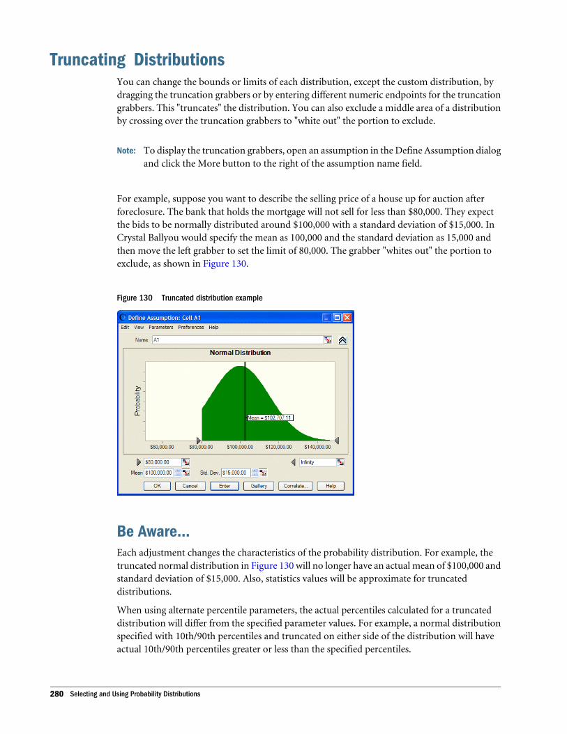
Truncating DistributionsYou can change the bounds or limits of each distribution, except the custom distribution, bydragging the truncation grabbers or by entering different numeric endpoints for the truncationgrabbers. This "truncates" the distribution. You can also exclude a middle area of a distributionby crossing over the truncation grabbers to "white out" the portion to exclude.
Note: To display the truncation grabbers, open an assumption in the Define Assumption dialogand click the More button to the right of the assumption name field.
For example, suppose you want to describe the selling price of a house up for auction afterforeclosure. The bank that holds the mortgage will not sell for less than $80,000. They expectthe bids to be normally distributed around $100,000 with a standard deviation of $15,000. InCrystal Ballyou would specify the mean as 100,000 and the standard deviation as 15,000 andthen move the left grabber to set the limit of 80,000. The grabber "whites out" the portion toexclude, as shown in Figure 130.
Figure 130 Truncated distribution example
Be Aware...Each adjustment changes the characteristics of the probability distribution. For example, thetruncated normal distribution in Figure 130 will no longer have an actual mean of $100,000 andstandard deviation of $15,000. Also, statistics values will be approximate for truncateddistributions.
When using alternate percentile parameters, the actual percentiles calculated for a truncateddistribution will differ from the specified parameter values. For example, a normal distributionspecified with 10th/90th percentiles and truncated on either side of the distribution will haveactual 10th/90th percentiles greater or less than the specified percentiles.
280 Selecting and Using Probability Distributions
Showing the mean line of the distribution is useful when truncating distributions. However, themean line value might differ from the Mean parameter field. The mean line shows the actualmean of the truncated distribution while the Mean parameter field shows the mean of thecomplete distribution.
Comparing DistributionsMany of the distributions discussed in this chapter are related to one another in various ways.For example, the geometric distribution is related to the binomial distribution. The geometricdistribution represents the number of trials until the next success while the binomial representsthe number of successes in a fixed number of trials. Similarly, the Poisson distribution is relatedto the exponential distribution. The exponential distribution represents the amount of time untilthe next occurrence of an event while the Poisson distribution represents the number of timesan event occurs within a given period of time.
In some situations, as when the number of trials for the binomial distribution becomes verylarge, the normal and binomial distributions become similar. For these two distributions, as thenumber of binomial trials approaches infinity, the probabilities become identical for any giveninterval. For this reason, you can use the normal distribution to approximate the binomialdistribution when the number of trials becomes too large for Crystal Ball to handle (more than1000 trials). You also can use the Poisson distribution to approximate the binomial distributionwhen the number of trials is large, but there is little advantage to this since Crystal Ball takes acomparable amount of time to compute both distributions.
Likewise, the normal and Student’s t distributions are related. With Degrees of Freedom, then30, Student’s t closely approximates the normal distribution.
The binomial and hypergeometric distributions are also closely related. As the number of trialsand the population size increase, the hypergeometric trials tend to become independent like thebinomial trials: the outcome of a single trial has a negligible effect on the probabilities ofsuccessive observations. The differences between these two types of distributions becomeimportant only when you are analyzing samples from relatively small populations. As with thePoisson and binomial distributions, Crystal Ball requires a similar amount of time to computeboth the binomial and hypergeometric distributions.
The yes-no distribution is simply the binomial distribution with Trials = 1.
The Weibull distribution is flexible. Actually, it consists of a family of distributions that canassume the properties of several distributions. When the Weibull shape parameter is 1.0, theWeibull distribution is identical to the exponential distribution. The Weibull location parameterlets you set up an exponential distribution to start at a location other than 0.0. When the shapeparameter is less than 1.0, the Weibull distribution becomes a steeply declining curve. Amanufacturer might find this effect useful in describing part failures during a burn-in period.When the shape parameter is equal to 2.0, a special form of the Weibull distribution, called theRayleigh distribution, results. A researcher might find the Rayleigh distribution useful foranalyzing noise problems in communication systems or for use in reliability studies. When theshape parameter is set to 3.25, the Weibull distribution approximates the shape of the normaldistribution; however, for applications when the normal distribution is appropriate, us it insteadof the Weibull distribution.
Comparing Distributions 281
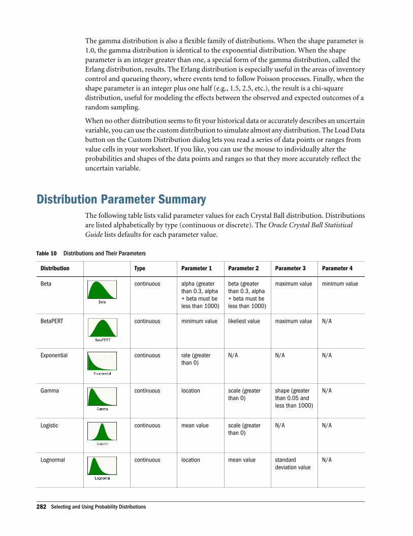
The gamma distribution is also a flexible family of distributions. When the shape parameter is1.0, the gamma distribution is identical to the exponential distribution. When the shapeparameter is an integer greater than one, a special form of the gamma distribution, called theErlang distribution, results. The Erlang distribution is especially useful in the areas of inventorycontrol and queueing theory, where events tend to follow Poisson processes. Finally, when theshape parameter is an integer plus one half (e.g., 1.5, 2.5, etc.), the result is a chi-squaredistribution, useful for modeling the effects between the observed and expected outcomes of arandom sampling.
When no other distribution seems to fit your historical data or accurately describes an uncertainvariable, you can use the custom distribution to simulate almost any distribution. The Load Databutton on the Custom Distribution dialog lets you read a series of data points or ranges fromvalue cells in your worksheet. If you like, you can use the mouse to individually alter theprobabilities and shapes of the data points and ranges so that they more accurately reflect theuncertain variable.
Distribution Parameter SummaryThe following table lists valid parameter values for each Crystal Ball distribution. Distributionsare listed alphabetically by type (continuous or discrete). The Oracle Crystal Ball StatisticalGuide lists defaults for each parameter value.
Table 10 Distributions and Their Parameters
Distribution Type Parameter 1 Parameter 2 Parameter 3 Parameter 4
Beta continuous alpha (greaterthan 0.3, alpha+ beta must beless than 1000)
beta (greaterthan 0.3, alpha+ beta must beless than 1000)
maximum value minimum value
BetaPERT continuous minimum value likeliest value maximum value N/A
Exponential continuous rate (greaterthan 0)
N/A N/A N/A
Gamma continuous location scale (greaterthan 0)
shape (greaterthan 0.05 andless than 1000)
N/A
Logistic continuous mean value scale (greaterthan 0)
N/A N/A
Lognormal continuous location mean value standarddeviation value
N/A
282 Selecting and Using Probability Distributions
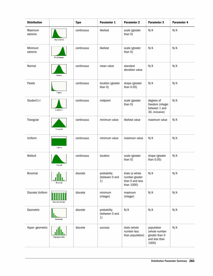
Distribution Type Parameter 1 Parameter 2 Parameter 3 Parameter 4
Maximumextreme
continuous likeliest scale (greaterthan 0)
N/A N/A
Minimumextreme
continuous likeliest scale (greaterthan 0)
N/A N/A
Normal continuous mean value standarddeviation value
N/A N/A
Pareto continuous location (greaterthan 0)
shape (greaterthan 0.05)
N/A N/A
Student’s t continuous midpoint scale (greaterthan 0)
degrees offreedom (integerbetween 1 and30, inclusive)
N/A
Triangular continuous minimum value likeliest value maximum value N/A
Uniform continuous minimum value maximum value N/A N/A
Weibull continuous location scale (greaterthan 0)
shape (greaterthan 0.05)
N/A
Binomial discrete probability(between 0 and1)
trials (a wholenumber greaterthan 0 and lessthan 1000)
N/A N/A
Discrete Uniform discrete minimum(integer)
maximum(integer)
N/A N/A
Geometric discrete probability(between 0 and1)
N/A N/A N/A
Hyper- geometric discrete success trials (wholenumber lessthan population)
population(whole numbergreater than 0and less than1000)
N/A
Distribution Parameter Summary 283
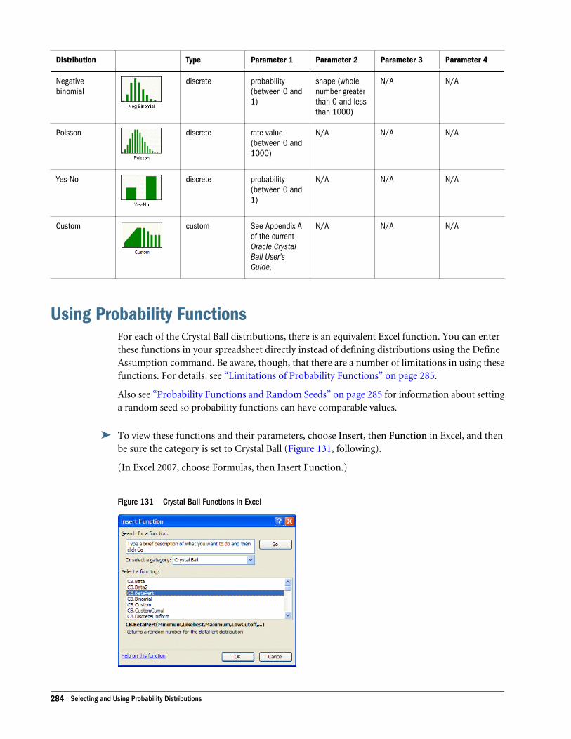
Distribution Type Parameter 1 Parameter 2 Parameter 3 Parameter 4
Negativebinomial
discrete probability(between 0 and1)
shape (wholenumber greaterthan 0 and lessthan 1000)
N/A N/A
Poisson discrete rate value(between 0 and1000)
N/A N/A N/A
Yes-No discrete probability(between 0 and1)
N/A N/A N/A
Custom custom See Appendix Aof the currentOracle CrystalBall User'sGuide.
N/A N/A N/A
Using Probability FunctionsFor each of the Crystal Ball distributions, there is an equivalent Excel function. You can enterthese functions in your spreadsheet directly instead of defining distributions using the DefineAssumption command. Be aware, though, that there are a number of limitations in using thesefunctions. For details, see “Limitations of Probability Functions” on page 285.
Also see “Probability Functions and Random Seeds” on page 285 for information about settinga random seed so probability functions can have comparable values.
ä To view these functions and their parameters, choose Insert, then Function in Excel, and thenbe sure the category is set to Crystal Ball (Figure 131, following).
(In Excel 2007, choose Formulas, then Insert Function.)
Figure 131 Crystal Ball Functions in Excel
284 Selecting and Using Probability Distributions
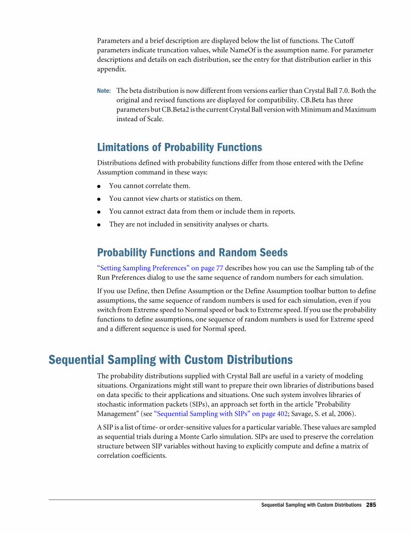
Parameters and a brief description are displayed below the list of functions. The Cutoffparameters indicate truncation values, while NameOf is the assumption name. For parameterdescriptions and details on each distribution, see the entry for that distribution earlier in thisappendix.
Note: The beta distribution is now different from versions earlier than Crystal Ball 7.0. Both theoriginal and revised functions are displayed for compatibility. CB.Beta has threeparameters but CB.Beta2 is the current Crystal Ball version with Minimum and Maximuminstead of Scale.
Limitations of Probability FunctionsDistributions defined with probability functions differ from those entered with the DefineAssumption command in these ways:
l You cannot correlate them.
l You cannot view charts or statistics on them.
l You cannot extract data from them or include them in reports.
l They are not included in sensitivity analyses or charts.
Probability Functions and Random Seeds“Setting Sampling Preferences” on page 77 describes how you can use the Sampling tab of theRun Preferences dialog to use the same sequence of random numbers for each simulation.
If you use Define, then Define Assumption or the Define Assumption toolbar button to defineassumptions, the same sequence of random numbers is used for each simulation, even if youswitch from Extreme speed to Normal speed or back to Extreme speed. If you use the probabilityfunctions to define assumptions, one sequence of random numbers is used for Extreme speedand a different sequence is used for Normal speed.
Sequential Sampling with Custom DistributionsThe probability distributions supplied with Crystal Ball are useful in a variety of modelingsituations. Organizations might still want to prepare their own libraries of distributions basedon data specific to their applications and situations. One such system involves libraries ofstochastic information packets (SIPs), an approach set forth in the article "ProbabilityManagement" (see “Sequential Sampling with SIPs” on page 402; Savage, S. et al, 2006).
A SIP is a list of time- or order-sensitive values for a particular variable. These values are sampledas sequential trials during a Monte Carlo simulation. SIPs are used to preserve the correlationstructure between SIP variables without having to explicitly compute and define a matrix ofcorrelation coefficients.
Sequential Sampling with Custom Distributions 285
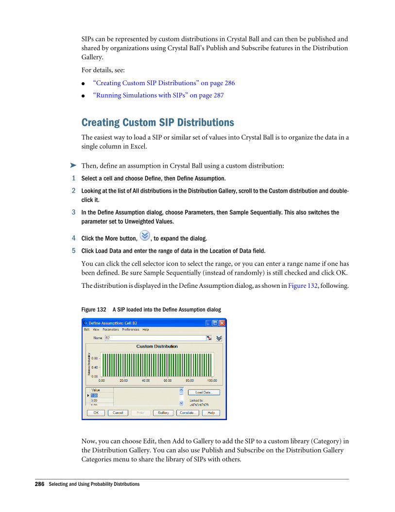
SIPs can be represented by custom distributions in Crystal Ball and can then be published andshared by organizations using Crystal Ball’s Publish and Subscribe features in the DistributionGallery.
For details, see:
l “Creating Custom SIP Distributions” on page 286
l “Running Simulations with SIPs” on page 287
Creating Custom SIP DistributionsThe easiest way to load a SIP or similar set of values into Crystal Ball is to organize the data in asingle column in Excel.
ä Then, define an assumption in Crystal Ball using a custom distribution:
1 Select a cell and choose Define, then Define Assumption.
2 Looking at the list of All distributions in the Distribution Gallery, scroll to the Custom distribution and double-click it.
3 In the Define Assumption dialog, choose Parameters, then Sample Sequentially. This also switches theparameter set to Unweighted Values.
4 Click the More button, , to expand the dialog.
5 Click Load Data and enter the range of data in the Location of Data field.
You can click the cell selector icon to select the range, or you can enter a range name if one hasbeen defined. Be sure Sample Sequentially (instead of randomly) is still checked and click OK.
The distribution is displayed in the Define Assumption dialog, as shown in Figure 132, following.
Figure 132 A SIP loaded into the Define Assumption dialog
Now, you can choose Edit, then Add to Gallery to add the SIP to a custom library (Category) inthe Distribution Gallery. You can also use Publish and Subscribe on the Distribution GalleryCategories menu to share the library of SIPs with others.
286 Selecting and Using Probability Distributions
Running Simulations with SIPsTo run a simulation with one or more SIPs, define assumptions in your model as usual, pullingin SIPs from a library (Category) in the Distribution Gallery as needed. When the simulationruns, Crystal Ball samples the SIP values sequentially instead of randomly. If the simulation hasmore trials than there are values in the SIP, sampling wraps around to the first value of thedistribution. If you are using several SIPs with different numbers of values, a warning is displayed.You can either continue, knowing that mismatched values will be sampled together aftersampling wraps for one SIP but not the other, or you can cancel the simulation and correct theproblem. You can also run fewer trials so that sampling doesn’t need to wrap for any SIP.
Correlations are not allowed for assumptions defined as SIPs, since the correlation structuresare implicitly defined for them. Warnings are displayed if correlations are defined for them.
Two Crystal Ball Developer Kit calls, CB.DefineAssumND and CB.GetAssum, support the newparameter for sequential sampling. The Developer Kit constant is called cbAsmIsSequential, aBoolean type.
Sequential Sampling with Custom Distributions 287

288 Selecting and Using Probability Distributions
BAccessibility
In This Appendix
Introduction... . . . . . . . . . . . . . . . . . . . . . . . . . . . . . . . . . . . . . . . . . . . . . . . . . . . . . . . . . . . . . . . . . . . . . . . . . . . . . . . . . . . . . . . . . . . . . . . . . . . . . . . . . . . . . . . . . . . . 289
Enabling Accessibility for Crystal Ball . . . . . . . . . . . . . . . . . . . . . . . . . . . . . . . . . . . . . . . . . . . . . . . . . . . . . . . . . . . . . . . . . . . . . . . . . . . . . . . . . . . . . . . . . . 289
Using the Tab and Arrow Keys in the Crystal Ball User Interface ... . . . . . . . . . . . . . . . . . . . . . . . . . . . . . . . . . . . . . . . . . . . . . . . . . . . . . . . . . 289
Toolbar and Menu Commands: Excel 2003 or Earlier . . . . . . . . . . . . . . . . . . . . . . . . . . . . . . . . . . . . . . . . . . . . . . . . . . . . . . . . . . . . . . . . . . . . . . . . 290
Using Crystal Ball in Excel 2007 ... . . . . . . . . . . . . . . . . . . . . . . . . . . . . . . . . . . . . . . . . . . . . . . . . . . . . . . . . . . . . . . . . . . . . . . . . . . . . . . . . . . . . . . . . . . . . 301
IntroductionThis appendix describes the accessibility features of Crystal Ball, including keyboard equivalentsfor application commands.
Enabling Accessibility for Crystal BallYou do not need to enable accessibility specifically for Crystal Ball; it is always in accessible mode.Crystal Ball output can be extracted to Excel spreadsheets and pasted into PowerPoint slides,which are accessible through Microsoft Office. For information about Excel or PowerPointaccessibility, refer to Microsoft Office product documentation.
Using the Tab and Arrow Keys in the Crystal Ball User InterfaceThe main Crystal Ball menubar and menu commands are accessed with shortcut keys. After amenu is open, the Tab key or Down Arrow key highlights commands in a circular sequence(tabbing from the last item moves focus to the first item). Using Shift+Tab or the Up Arrowhighlights commands in the opposite direction.
Default tab order in the Crystal Ball dialogs flows from left to right, top to bottom. Tab can beused to access the first item of a subwindow in a dialog, but then arrow keys are needed to moveto additional items. For example, in the Distribution Gallery, Alt+b displays six basicdistributions and places the focus on one of them. Using one of the arrow keys moves focus toan adjacent distribution. Tab moves focus to the OK button at the bottom of the dialog.
Introduction 289
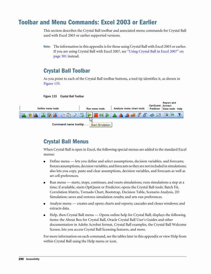
Toolbar and Menu Commands: Excel 2003 or EarlierThis section describes the Crystal Ball toolbar and associated menu commands for Crystal Ballused with Excel 2003 or earlier supported versions.
Note: The information in this appendix is for those using Crystal Ball with Excel 2003 or earlier.If you are using Crystal Ball with Excel 2007, see “Using Crystal Ball in Excel 2007” onpage 301 instead.
Crystal Ball ToolbarAs you point to each of the Crystal Ball toolbar buttons, a tool tip identifies it, as shown inFigure 133.
Figure 133 Crystal Ball Toolbar
Crystal Ball MenusWhen Crystal Ball is open in Excel, the following special menus are added to the standard Excelmenus:
l Define menu — lets you define and select assumptions, decision variables, and forecasts;freezes assumptions, decision variables, and forecasts so they are not included in simulations;also lets you copy, paste and clear assumptions, decision variables, and forecasts as well asset cell preferences.
l Run menu — starts, stops, continues, and resets simulations; runs simulations a step at atime; if available, starts OptQuest or Predictor; opens the Crystal Ball tools: Batch Fit,Correlation Matrix, Tornado Chart, Bootstrap, Decision Table, Scenario Analysis, 2DSimulation; saves and restores simulation results; and sets run preferences.
l Analyze menu — creates and opens charts and reports; cascades and closes windows; andextracts data.
l Help, then Crystal Ball menu — Opens online help for Crystal Ball; displays the followingitems: the About Box for Crystal Ball, Oracle Crystal Ball User's Guides and otherdocumentation in Adobe Acrobat format, Crystal Ball examples, the Crystal Ball WelcomeScreen, lets you access Crystal Ball licensing features, and more.
For more information on each command, see the tables later in this appendix or view Help fromwithin Crystal Ball using the Help menu or icon.
290 Accessibility
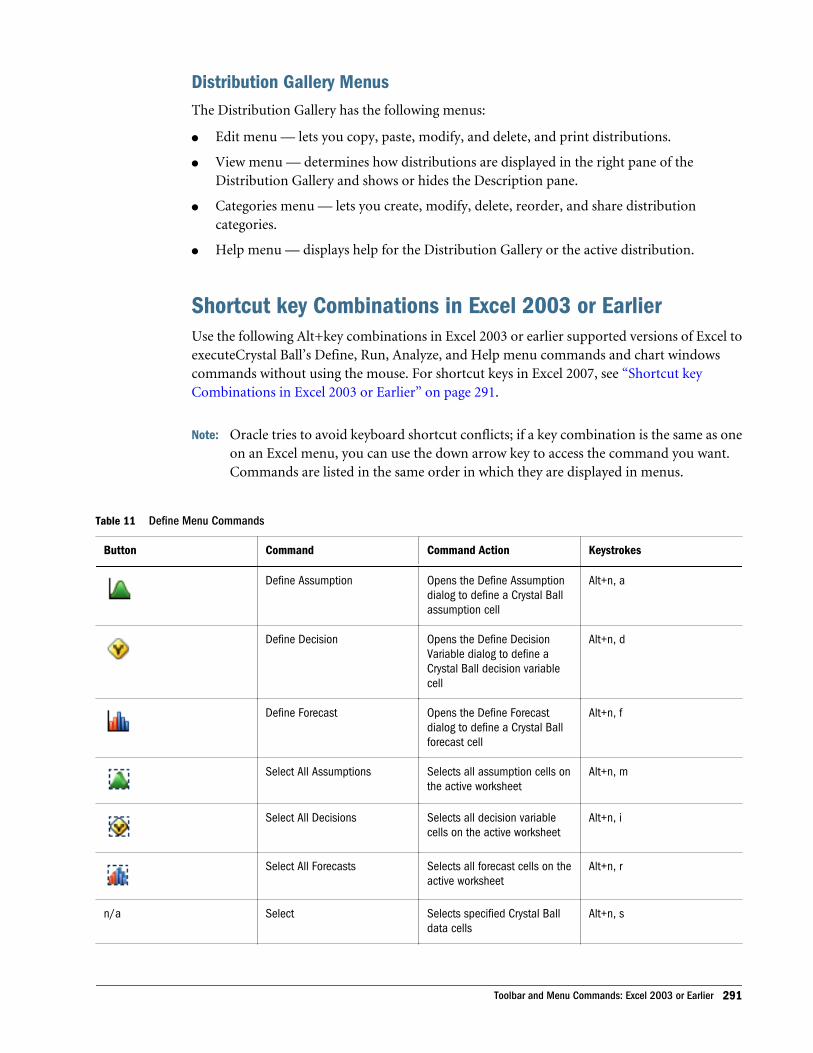
Distribution Gallery MenusThe Distribution Gallery has the following menus:
l Edit menu — lets you copy, paste, modify, and delete, and print distributions.
l View menu — determines how distributions are displayed in the right pane of theDistribution Gallery and shows or hides the Description pane.
l Categories menu — lets you create, modify, delete, reorder, and share distributioncategories.
l Help menu — displays help for the Distribution Gallery or the active distribution.
Shortcut key Combinations in Excel 2003 or EarlierUse the following Alt+key combinations in Excel 2003 or earlier supported versions of Excel toexecuteCrystal Ball’s Define, Run, Analyze, and Help menu commands and chart windowscommands without using the mouse. For shortcut keys in Excel 2007, see “Shortcut keyCombinations in Excel 2003 or Earlier” on page 291.
Note: Oracle tries to avoid keyboard shortcut conflicts; if a key combination is the same as oneon an Excel menu, you can use the down arrow key to access the command you want.Commands are listed in the same order in which they are displayed in menus.
Table 11 Define Menu Commands
Button Command Command Action Keystrokes
Define Assumption Opens the Define Assumptiondialog to define a Crystal Ballassumption cell
Alt+n, a
Define Decision Opens the Define DecisionVariable dialog to define aCrystal Ball decision variablecell
Alt+n, d
Define Forecast Opens the Define Forecastdialog to define a Crystal Ballforecast cell
Alt+n, f
Select All Assumptions Selects all assumption cells onthe active worksheet
Alt+n, m
Select All Decisions Selects all decision variablecells on the active worksheet
Alt+n, i
Select All Forecasts Selects all forecast cells on theactive worksheet
Alt+n, r
n/a Select Selects specified Crystal Balldata cells
Alt+n, s
Toolbar and Menu Commands: Excel 2003 or Earlier 291
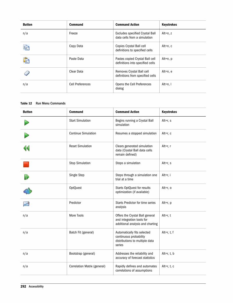
Button Command Command Action Keystrokes
n/a Freeze Excludes specified Crystal Balldata cells from a simulation
Alt+n, z
Copy Data Copies Crystal Ball celldefinitions to specified cells
Alt+n, c
Paste Data Pastes copied Crystal Ball celldefinitions into specified cells
Alt+n, p
Clear Data Removes Crystal Ball celldefinitions from specified cells
Alt+n, e
n/a Cell Preferences Opens the Cell Preferencesdialog
Alt+n, l
Table 12 Run Menu Commands
Button Command Command Action Keystrokes
Start Simulation Begins running a Crystal Ballsimulation
Alt+r, s
Continue Simulation Resumes a stopped simulation Alt+r, c
Reset Simulation Clears generated simulationdata (Crystal Ball data cellsremain defined)
Alt+r, r
Stop Simulation Stops a simulation Alt+r, s
Single Step Steps through a simulation onetrial at a time
Alt+r, i
OptQuest Starts OptQuest for resultsoptimization (if available)
Alt+r, o
Predictor Starts Predictor for time seriesanalysis
Alt+r, p
n/a More Tools Offers the Crystal Ball generaland integration tools foradditional analysis and charting
Alt+r, t
n/a Batch Fit (general) Automatically fits selectedcontinuous probabilitydistributions to multiple dataseries
Alt+r, t, f
n/a Bootstrap (general) Addresses the reliability andaccuracy of forecast statistics
Alt+r, t, b
n/a Correlation Matrix (general) Rapidly defines and automatescorrelations of assumptions
Alt+r, t, c
292 Accessibility
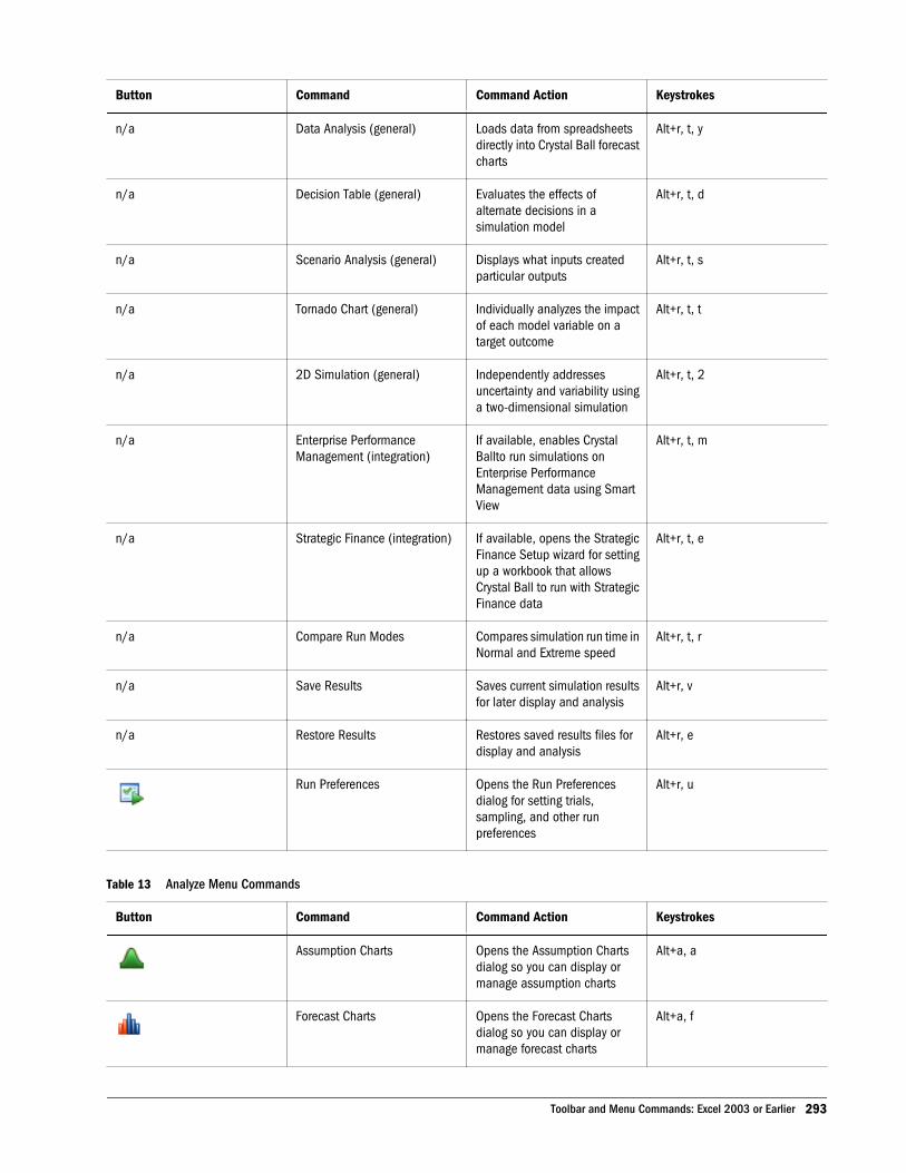
Button Command Command Action Keystrokes
n/a Data Analysis (general) Loads data from spreadsheetsdirectly into Crystal Ball forecastcharts
Alt+r, t, y
n/a Decision Table (general) Evaluates the effects ofalternate decisions in asimulation model
Alt+r, t, d
n/a Scenario Analysis (general) Displays what inputs createdparticular outputs
Alt+r, t, s
n/a Tornado Chart (general) Individually analyzes the impactof each model variable on atarget outcome
Alt+r, t, t
n/a 2D Simulation (general) Independently addressesuncertainty and variability usinga two-dimensional simulation
Alt+r, t, 2
n/a Enterprise PerformanceManagement (integration)
If available, enables CrystalBallto run simulations onEnterprise PerformanceManagement data using SmartView
Alt+r, t, m
n/a Strategic Finance (integration) If available, opens the StrategicFinance Setup wizard for settingup a workbook that allowsCrystal Ball to run with StrategicFinance data
Alt+r, t, e
n/a Compare Run Modes Compares simulation run time inNormal and Extreme speed
Alt+r, t, r
n/a Save Results Saves current simulation resultsfor later display and analysis
Alt+r, v
n/a Restore Results Restores saved results files fordisplay and analysis
Alt+r, e
Run Preferences Opens the Run Preferencesdialog for setting trials,sampling, and other runpreferences
Alt+r, u
Table 13 Analyze Menu Commands
Button Command Command Action Keystrokes
Assumption Charts Opens the Assumption Chartsdialog so you can display ormanage assumption charts
Alt+a, a
Forecast Charts Opens the Forecast Chartsdialog so you can display ormanage forecast charts
Alt+a, f
Toolbar and Menu Commands: Excel 2003 or Earlier 293
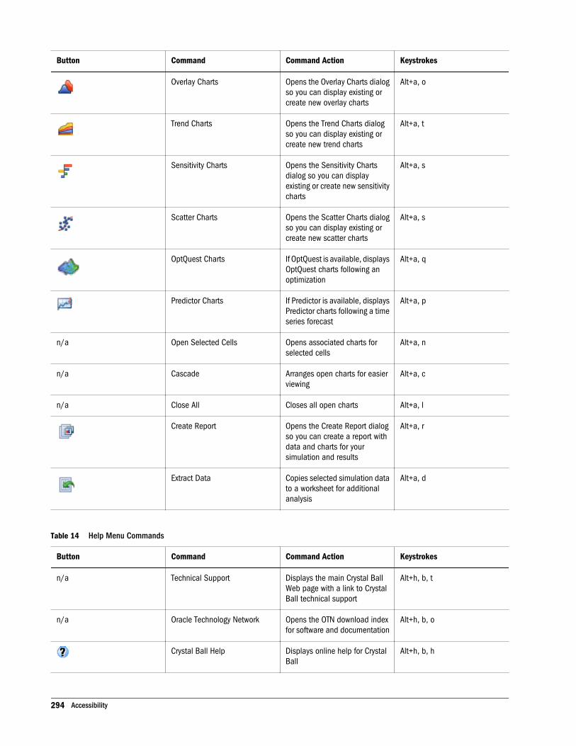
Button Command Command Action Keystrokes
Overlay Charts Opens the Overlay Charts dialogso you can display existing orcreate new overlay charts
Alt+a, o
Trend Charts Opens the Trend Charts dialogso you can display existing orcreate new trend charts
Alt+a, t
Sensitivity Charts Opens the Sensitivity Chartsdialog so you can displayexisting or create new sensitivitycharts
Alt+a, s
Scatter Charts Opens the Scatter Charts dialogso you can display existing orcreate new scatter charts
Alt+a, s
OptQuest Charts If OptQuest is available, displaysOptQuest charts following anoptimization
Alt+a, q
Predictor Charts If Predictor is available, displaysPredictor charts following a timeseries forecast
Alt+a, p
n/a Open Selected Cells Opens associated charts forselected cells
Alt+a, n
n/a Cascade Arranges open charts for easierviewing
Alt+a, c
n/a Close All Closes all open charts Alt+a, l
Create Report Opens the Create Report dialogso you can create a report withdata and charts for yoursimulation and results
Alt+a, r
Extract Data Copies selected simulation datato a worksheet for additionalanalysis
Alt+a, d
Table 14 Help Menu Commands
Button Command Command Action Keystrokes
n/a Technical Support Displays the main Crystal BallWeb page with a link to CrystalBall technical support
Alt+h, b, t
n/a Oracle Technology Network Opens the OTN download indexfor software and documentation
Alt+h, b, o
Crystal Ball Help Displays online help for CrystalBall
Alt+h, b, h
294 Accessibility
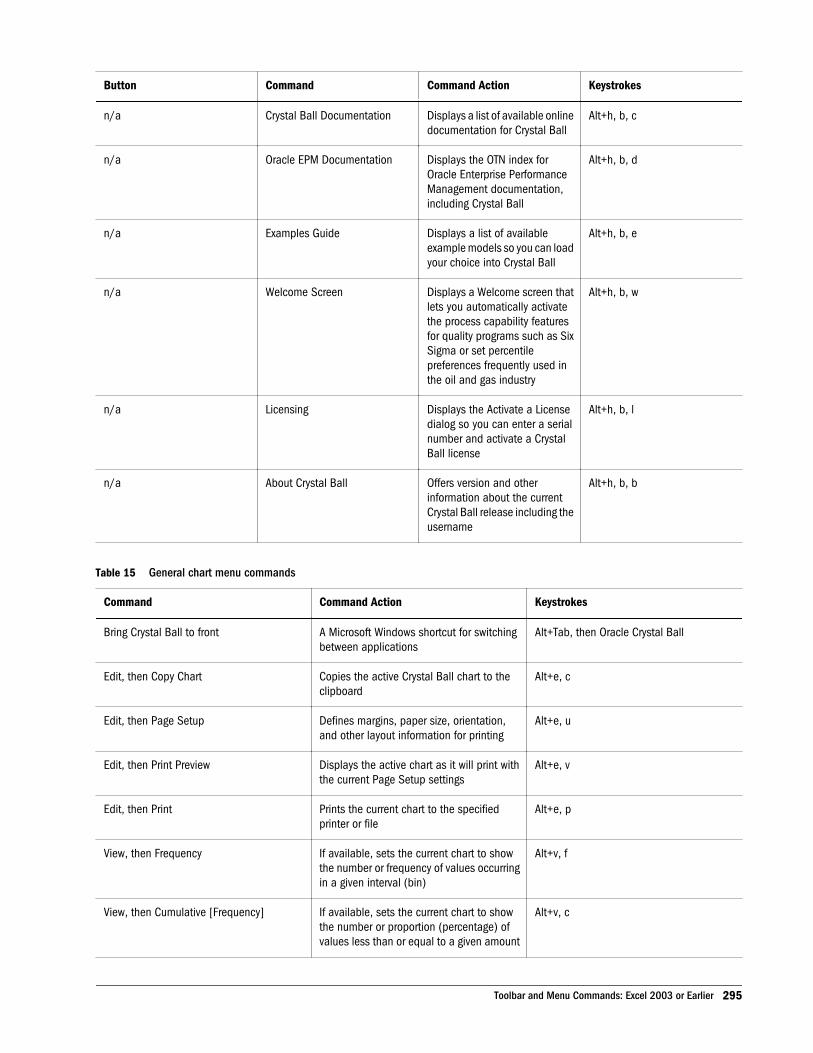
Button Command Command Action Keystrokes
n/a Crystal Ball Documentation Displays a list of available onlinedocumentation for Crystal Ball
Alt+h, b, c
n/a Oracle EPM Documentation Displays the OTN index forOracle Enterprise PerformanceManagement documentation,including Crystal Ball
Alt+h, b, d
n/a Examples Guide Displays a list of availableexample models so you can loadyour choice into Crystal Ball
Alt+h, b, e
n/a Welcome Screen Displays a Welcome screen thatlets you automatically activatethe process capability featuresfor quality programs such as SixSigma or set percentilepreferences frequently used inthe oil and gas industry
Alt+h, b, w
n/a Licensing Displays the Activate a Licensedialog so you can enter a serialnumber and activate a CrystalBall license
Alt+h, b, l
n/a About Crystal Ball Offers version and otherinformation about the currentCrystal Ball release including theusername
Alt+h, b, b
Table 15 General chart menu commands
Command Command Action Keystrokes
Bring Crystal Ball to front A Microsoft Windows shortcut for switchingbetween applications
Alt+Tab, then Oracle Crystal Ball
Edit, then Copy Chart Copies the active Crystal Ball chart to theclipboard
Alt+e, c
Edit, then Page Setup Defines margins, paper size, orientation,and other layout information for printing
Alt+e, u
Edit, then Print Preview Displays the active chart as it will print withthe current Page Setup settings
Alt+e, v
Edit, then Print Prints the current chart to the specifiedprinter or file
Alt+e, p
View, then Frequency If available, sets the current chart to showthe number or frequency of values occurringin a given interval (bin)
Alt+v, f
View, then Cumulative [Frequency] If available, sets the current chart to showthe number or proportion (percentage) ofvalues less than or equal to a given amount
Alt+v, c
Toolbar and Menu Commands: Excel 2003 or Earlier 295
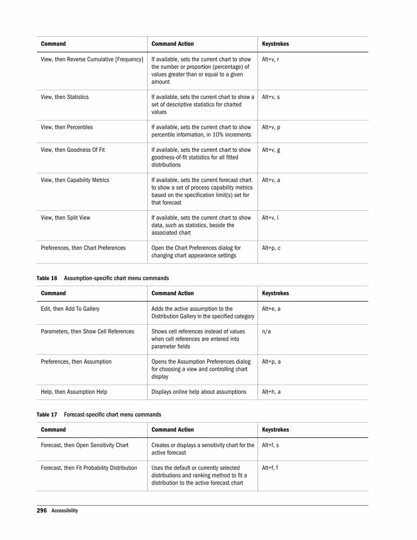
Command Command Action Keystrokes
View, then Reverse Cumulative [Frequency] If available, sets the current chart to showthe number or proportion (percentage) ofvalues greater than or equal to a givenamount
Alt+v, r
View, then Statistics If available, sets the current chart to show aset of descriptive statistics for chartedvalues
Alt+v, s
View, then Percentiles If available, sets the current chart to showpercentile information, in 10% increments
Alt+v, p
View, then Goodness Of Fit If available, sets the current chart to showgoodness-of-fit statistics for all fitteddistributions
Alt+v, g
View, then Capability Metrics If available, sets the current forecast chartto show a set of process capability metricsbased on the specification limit(s) set forthat forecast
Alt+v, a
View, then Split View If available, sets the current chart to showdata, such as statistics, beside theassociated chart
Alt+v, l
Preferences, then Chart Preferences Open the Chart Preferences dialog forchanging chart appearance settings
Alt+p, c
Table 16 Assumption-specific chart menu commands
Command Command Action Keystrokes
Edit, then Add To Gallery Adds the active assumption to theDistribution Gallery in the specified category
Alt+e, a
Parameters, then Show Cell References Shows cell references instead of valueswhen cell references are entered intoparameter fields
n/a
Preferences, then Assumption Opens the Assumption Preferences dialogfor choosing a view and controlling chartdisplay
Alt+p, a
Help, then Assumption Help Displays online help about assumptions Alt+h, a
Table 17 Forecast-specific chart menu commands
Command Command Action Keystrokes
Forecast, then Open Sensitivity Chart Creates or displays a sensitivity chart for theactive forecast
Alt+f, s
Forecast, then Fit Probability Distribution Uses the default or currently selecteddistributions and ranking method to fit adistribution to the active forecast chart
Alt+f, f
296 Accessibility
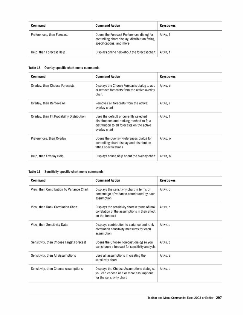
Command Command Action Keystrokes
Preferences, then Forecast Opens the Forecast Preferences dialog forcontrolling chart display, distribution fittingspecifications, and more
Alt+p, f
Help, then Forecast Help Displays online help about the forecast chart Alt+h, f
Table 18 Overlay-specific chart menu commands
Command Command Action Keystrokes
Overlay, then Choose Forecasts Displays the Choose Forecasts dialog to addor remove forecasts from the active overlaychart
Alt+o, c
Overlay, then Remove All Removes all forecasts from the activeoverlay chart
Alt+o, r
Overlay, then Fit Probability Distribution Uses the default or currently selecteddistributions and ranking method to fit adistribution to all forecasts on the activeoverlay chart
Alt+o, f
Preferences, then Overlay Opens the Overlay Preferences dialog forcontrolling chart display and distributionfitting specifications
Alt+p, o
Help, then Overlay Help Displays online help about the overlay chart Alt+h, o
Table 19 Sensitivity-specific chart menu commands
Command Command Action Keystrokes
View, then Contribution To Variance Chart Displays the sensitivity chart in terms ofpercentage of variance contributed by eachassumption
Alt+v, c
View, then Rank Correlation Chart Displays the sensitivity chart in terms of rankcorrelation of the assumptions in their effecton the forecast
Alt+v, r
View, then Sensitivity Data Displays contribution to variance and rankcorrelation sensitivity measures for eachassumption
Alt+v, s
Sensitivity, then Choose Target Forecast Opens the Choose Forecast dialog so youcan choose a forecast for sensitivity analysis
Alt+s, t
Sensitivity, then All Assumptions Uses all assumptions in creating thesensitivity chart
Alt+s, a
Sensitivity, then Choose Assumptions Displays the Choose Assumptions dialog soyou can choose one or more assumptionsfor the sensitivity chart
Alt+s, c
Toolbar and Menu Commands: Excel 2003 or Earlier 297
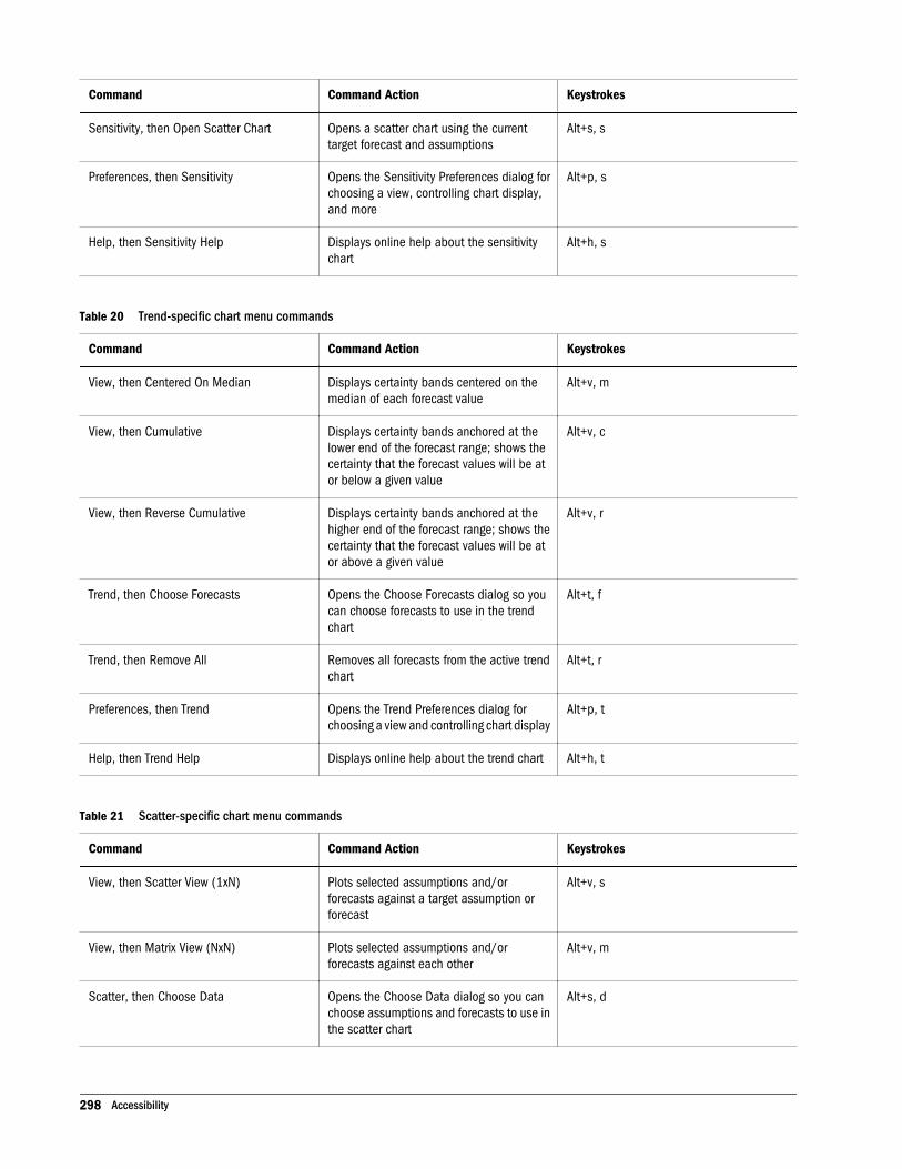
Command Command Action Keystrokes
Sensitivity, then Open Scatter Chart Opens a scatter chart using the currenttarget forecast and assumptions
Alt+s, s
Preferences, then Sensitivity Opens the Sensitivity Preferences dialog forchoosing a view, controlling chart display,and more
Alt+p, s
Help, then Sensitivity Help Displays online help about the sensitivitychart
Alt+h, s
Table 20 Trend-specific chart menu commands
Command Command Action Keystrokes
View, then Centered On Median Displays certainty bands centered on themedian of each forecast value
Alt+v, m
View, then Cumulative Displays certainty bands anchored at thelower end of the forecast range; shows thecertainty that the forecast values will be ator below a given value
Alt+v, c
View, then Reverse Cumulative Displays certainty bands anchored at thehigher end of the forecast range; shows thecertainty that the forecast values will be ator above a given value
Alt+v, r
Trend, then Choose Forecasts Opens the Choose Forecasts dialog so youcan choose forecasts to use in the trendchart
Alt+t, f
Trend, then Remove All Removes all forecasts from the active trendchart
Alt+t, r
Preferences, then Trend Opens the Trend Preferences dialog forchoosing a view and controlling chart display
Alt+p, t
Help, then Trend Help Displays online help about the trend chart Alt+h, t
Table 21 Scatter-specific chart menu commands
Command Command Action Keystrokes
View, then Scatter View (1xN) Plots selected assumptions and/orforecasts against a target assumption orforecast
Alt+v, s
View, then Matrix View (NxN) Plots selected assumptions and/orforecasts against each other
Alt+v, m
Scatter, then Choose Data Opens the Choose Data dialog so you canchoose assumptions and forecasts to use inthe scatter chart
Alt+s, d
298 Accessibility

Command Command Action Keystrokes
Scatter, then Remove All Removes all assumptions and forecastsfrom the active scatter chart
Alt+s, r
Preferences, then Scatter Opens the Scatter Preferences dialog forchoosing a view and controlling chart display
Alt+p, s
Help, then Scatter Help Displays online help about the scatter chart Alt+h, t
Distribution Gallery Shortcut Keys
Note: In Excel 2007, if you click the upper half of the Define Assumption icon, or if theassumption has already been defined, the Distribution Gallery opens. If you click the lowerhalf of the icon, a list of All, Basic, or Favorite distributions opens, depending on the activecategory in the Distribution Gallery.
You can use the keyboard to select distributions in the Distribution Gallery.
ä To do this:
1 Choose Define, then Define Assumption or click the Define Assumption button to open the Distribution
Gallery.
2 Type the first letter of the name of the target distribution, for example n for normal.
If more than one distribution starts with that letter, keep pressing to cycle through thedistributions.
3 When the target distribution is highlighted, type Alt+o (for OK) to open its Define Assumption dialog.
Or, you can press Alt+f to fit a distribution to it or Alt+c to cancel the selection and close thedialog.
ä To apply a shortcut key to a custom category:
1 Open the Crystal Ball Gallery.
2 Edit the category name:
For a new category, select Categories, then New. In the Name field, enter an ampersand (&)before a letter in your category name. That letter becomes the shortcut key. Click OK to save.
For an existing category, select Categories, then Properties, add the ampersand to the existingname, and click OK to save.
Each category should use a unique shortcut key. The shortcut keys for the default categories are:Alt+b for the Basic category, Alt+a for All, and Alt+i for Favorites.
Toolbar and Menu Commands: Excel 2003 or Earlier 299
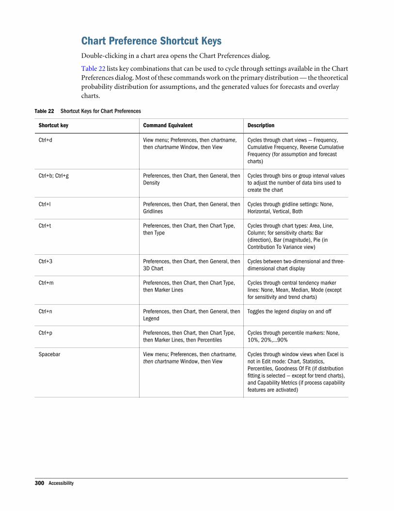
Chart Preference Shortcut KeysDouble-clicking in a chart area opens the Chart Preferences dialog.
Table 22 lists key combinations that can be used to cycle through settings available in the ChartPreferences dialog. Most of these commands work on the primary distribution — the theoreticalprobability distribution for assumptions, and the generated values for forecasts and overlaycharts.
Table 22 Shortcut Keys for Chart Preferences
Shortcut key Command Equivalent Description
Ctrl+d View menu; Preferences, then chartname,then chartname Window, then View
Cycles through chart views — Frequency,Cumulative Frequency, Reverse CumulativeFrequency (for assumption and forecastcharts)
Ctrl+b; Ctrl+g Preferences, then Chart, then General, thenDensity
Cycles through bins or group interval valuesto adjust the number of data bins used tocreate the chart
Ctrl+l Preferences, then Chart, then General, thenGridlines
Cycles through gridline settings: None,Horizontal, Vertical, Both
Ctrl+t Preferences, then Chart, then Chart Type,then Type
Cycles through chart types: Area, Line,Column; for sensitivity charts: Bar(direction), Bar (magnitude), Pie (inContribution To Variance view)
Ctrl+3 Preferences, then Chart, then General, then3D Chart
Cycles between two-dimensional and three-dimensional chart display
Ctrl+m Preferences, then Chart, then Chart Type,then Marker Lines
Cycles through central tendency markerlines: None, Mean, Median, Mode (exceptfor sensitivity and trend charts)
Ctrl+n Preferences, then Chart, then General, thenLegend
Toggles the legend display on and off
Ctrl+p Preferences, then Chart, then Chart Type,then Marker Lines, then Percentiles
Cycles through percentile markers: None,10%, 20%,…90%
Spacebar View menu; Preferences, then chartname,then chartname Window, then View
Cycles through window views when Excel isnot in Edit mode: Chart, Statistics,Percentiles, Goodness Of Fit (if distributionfitting is selected — except for trend charts),and Capability Metrics (if process capabilityfeatures are activated)
300 Accessibility
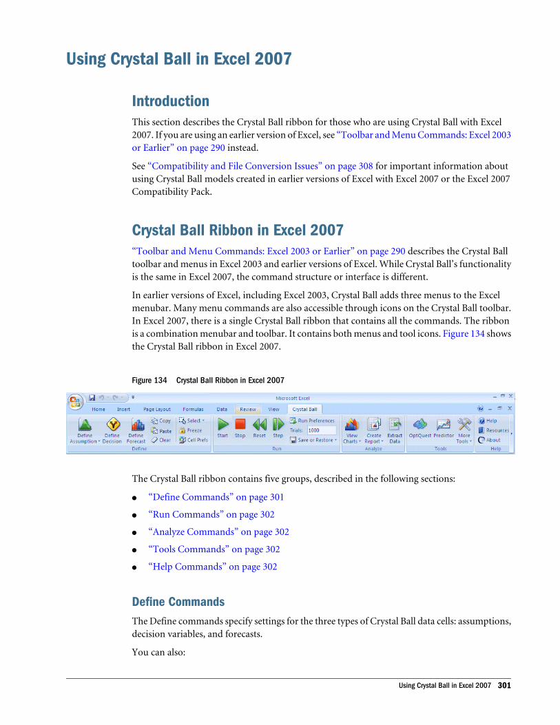
Using Crystal Ball in Excel 2007
IntroductionThis section describes the Crystal Ball ribbon for those who are using Crystal Ball with Excel2007. If you are using an earlier version of Excel, see “Toolbar and Menu Commands: Excel 2003or Earlier” on page 290 instead.
See “Compatibility and File Conversion Issues” on page 308 for important information aboutusing Crystal Ball models created in earlier versions of Excel with Excel 2007 or the Excel 2007Compatibility Pack.
Crystal Ball Ribbon in Excel 2007“Toolbar and Menu Commands: Excel 2003 or Earlier” on page 290 describes the Crystal Balltoolbar and menus in Excel 2003 and earlier versions of Excel. While Crystal Ball’s functionalityis the same in Excel 2007, the command structure or interface is different.
In earlier versions of Excel, including Excel 2003, Crystal Ball adds three menus to the Excelmenubar. Many menu commands are also accessible through icons on the Crystal Ball toolbar.In Excel 2007, there is a single Crystal Ball ribbon that contains all the commands. The ribbonis a combination menubar and toolbar. It contains both menus and tool icons. Figure 134 showsthe Crystal Ball ribbon in Excel 2007.
Figure 134 Crystal Ball Ribbon in Excel 2007
The Crystal Ball ribbon contains five groups, described in the following sections:
l “Define Commands” on page 301
l “Run Commands” on page 302
l “Analyze Commands” on page 302
l “Tools Commands” on page 302
l “Help Commands” on page 302
Define CommandsThe Define commands specify settings for the three types of Crystal Ball data cells: assumptions,decision variables, and forecasts.
You can also:
Using Crystal Ball in Excel 2007 301
l Set cell preferences
l Select Crystal Ball data cells
l Copy, paste, and clear Crystal Ball data
l Freeze data cells to exclude them from Crystal Ball simulations
Run CommandsYou can use the basic Run commands to start, stop, continue, reset, and single-step throughCrystal Ball simulations. You can use other Run commands to:
l Save or restore Crystal Ball simulation results
l Set run preferences, which control the number of trials, the sampling method, and othersimulation options
Analyze CommandsYou can use the Analyze commands to:
l Create and view Crystal Ball charts
l Create reports
l Extract data for external use
Tools CommandsYou can use the Tools commands to access the Crystal Ball tools, Predictor, and OptQuest withan appropriate license.
Help CommandsThe Help commands display online help, online documents, example models, the Crystal BallAbout Box, and more.
Shortcut Key Combinations in Excel 2007The following tables list Alt+key combinations in Excel 2007 so you can use the Define, Run,Analyze, and Help commands in the Crystal Ball ribbon without using the mouse:
l Table 23 on page 303
l Table 24 on page 304
l Table 25 on page 304
l Table 27 on page 307
For shortcut keys in Excel 2003, see “Shortcut key Combinations in Excel 2003 or Earlier” onpage 291.
302 Accessibility
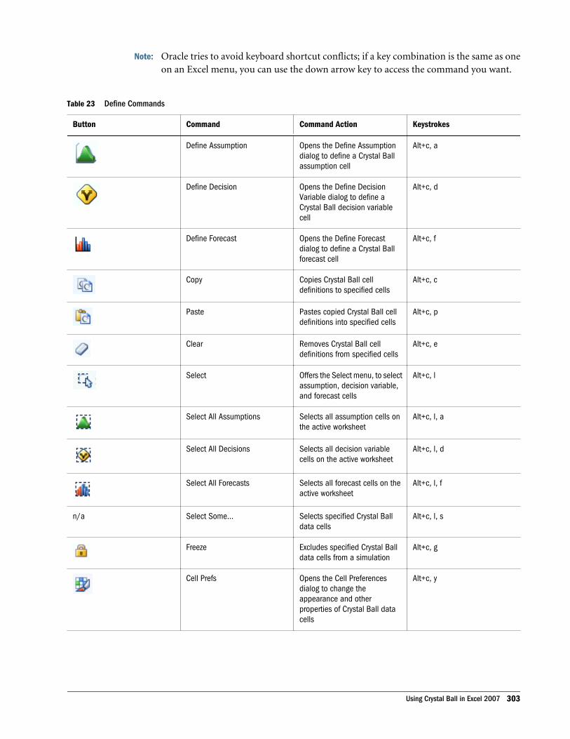
Note: Oracle tries to avoid keyboard shortcut conflicts; if a key combination is the same as oneon an Excel menu, you can use the down arrow key to access the command you want.
Table 23 Define Commands
Button Command Command Action Keystrokes
Define Assumption Opens the Define Assumptiondialog to define a Crystal Ballassumption cell
Alt+c, a
Define Decision Opens the Define DecisionVariable dialog to define aCrystal Ball decision variablecell
Alt+c, d
Define Forecast Opens the Define Forecastdialog to define a Crystal Ballforecast cell
Alt+c, f
Copy Copies Crystal Ball celldefinitions to specified cells
Alt+c, c
Paste Pastes copied Crystal Ball celldefinitions into specified cells
Alt+c, p
Clear Removes Crystal Ball celldefinitions from specified cells
Alt+c, e
Select Offers the Select menu, to selectassumption, decision variable,and forecast cells
Alt+c, l
Select All Assumptions Selects all assumption cells onthe active worksheet
Alt+c, l, a
Select All Decisions Selects all decision variablecells on the active worksheet
Alt+c, l, d
Select All Forecasts Selects all forecast cells on theactive worksheet
Alt+c, l, f
n/a Select Some... Selects specified Crystal Balldata cells
Alt+c, l, s
Freeze Excludes specified Crystal Balldata cells from a simulation
Alt+c, g
Cell Prefs Opens the Cell Preferencesdialog to change theappearance and otherproperties of Crystal Ball datacells
Alt+c, y
Using Crystal Ball in Excel 2007 303
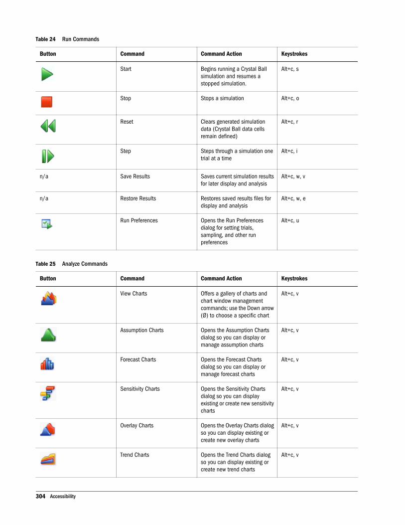
Table 24 Run Commands
Button Command Command Action Keystrokes
Start Begins running a Crystal Ballsimulation and resumes astopped simulation.
Alt+c, s
Stop Stops a simulation Alt+c, o
Reset Clears generated simulationdata (Crystal Ball data cellsremain defined)
Alt+c, r
Step Steps through a simulation onetrial at a time
Alt+c, i
n/a Save Results Saves current simulation resultsfor later display and analysis
Alt+c, w, v
n/a Restore Results Restores saved results files fordisplay and analysis
Alt+c, w, e
Run Preferences Opens the Run Preferencesdialog for setting trials,sampling, and other runpreferences
Alt+c, u
Table 25 Analyze Commands
Button Command Command Action Keystrokes
View Charts Offers a gallery of charts andchart window managementcommands; use the Down arrow(Ø) to choose a specific chart
Alt+c, v
Assumption Charts Opens the Assumption Chartsdialog so you can display ormanage assumption charts
Alt+c, v
Forecast Charts Opens the Forecast Chartsdialog so you can display ormanage forecast charts
Alt+c, v
Sensitivity Charts Opens the Sensitivity Chartsdialog so you can displayexisting or create new sensitivitycharts
Alt+c, v
Overlay Charts Opens the Overlay Charts dialogso you can display existing orcreate new overlay charts
Alt+c, v
Trend Charts Opens the Trend Charts dialogso you can display existing orcreate new trend charts
Alt+c, v
304 Accessibility
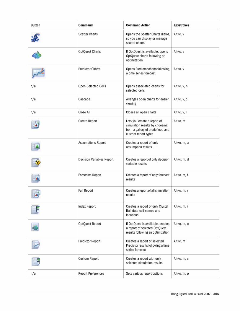
Button Command Command Action Keystrokes
Scatter Charts Opens the Scatter Charts dialogso you can display or managescatter charts
Alt+c, v
OptQuest Charts If OptQuest is available, opensOptQuest charts following anoptimization
Alt+c, v
Predictor Charts Opens Predictor charts followinga time series forecast
Alt+c, v
n/a Open Selected Cells Opens associated charts forselected cells
Alt+c, v, n
n/a Cascade Arranges open charts for easierviewing
Alt+c, v, c
n/a Close All Closes all open charts Alt+c, v, l
Create Report Lets you create a report ofsimulation results by choosingfrom a gallery of predefined andcustom report types
Alt+c, m
Assumptions Report Creates a report of onlyassumption results
Alt+c, m, a
Decision Variables Report Creates a report of only decisionvariable results
Alt+c, m, d
Forecasts Report Creates a report of only forecastresults
Alt+c, m, f
Full Report Creates a report of all simulationresults
Alt+c, m, r
Index Report Creates a report of only CrystalBall data cell names andlocations
Alt+c, m, i
OptQuest Report If OptQuest is available, createsa report of selected OptQuestresults following an optimization
Alt+c, m, o
Predictor Report Creates a report of selectedPredictor results following a timeseries forecast
Alt+c, m
Custom Report Creates a report with onlyselected simulation results
Alt+c, m, c
n/a Report Preferences Sets various report options Alt+c, m, p
Using Crystal Ball in Excel 2007 305
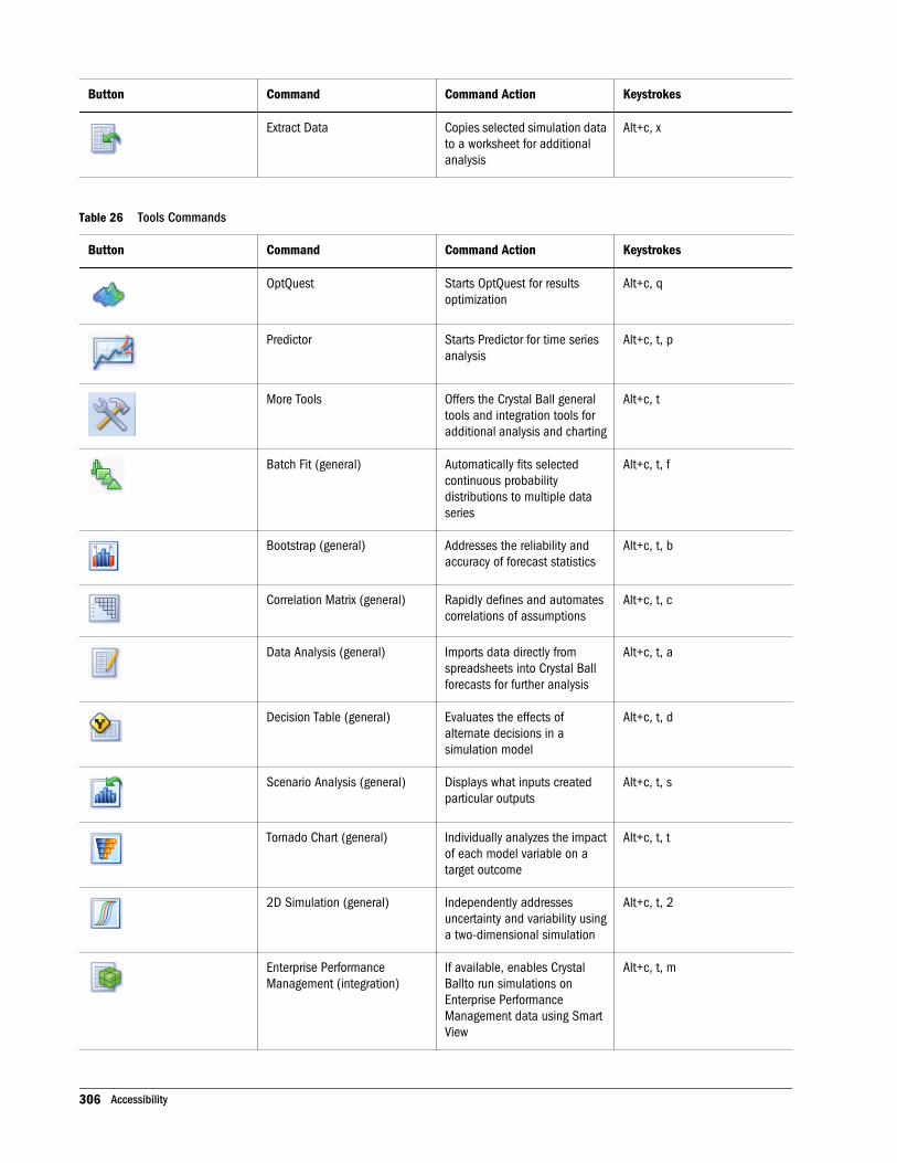
Button Command Command Action Keystrokes
Extract Data Copies selected simulation datato a worksheet for additionalanalysis
Alt+c, x
Table 26 Tools Commands
Button Command Command Action Keystrokes
OptQuest Starts OptQuest for resultsoptimization
Alt+c, q
Predictor Starts Predictor for time seriesanalysis
Alt+c, t, p
More Tools Offers the Crystal Ball generaltools and integration tools foradditional analysis and charting
Alt+c, t
Batch Fit (general) Automatically fits selectedcontinuous probabilitydistributions to multiple dataseries
Alt+c, t, f
Bootstrap (general) Addresses the reliability andaccuracy of forecast statistics
Alt+c, t, b
Correlation Matrix (general) Rapidly defines and automatescorrelations of assumptions
Alt+c, t, c
Data Analysis (general) Imports data directly fromspreadsheets into Crystal Ballforecasts for further analysis
Alt+c, t, a
Decision Table (general) Evaluates the effects ofalternate decisions in asimulation model
Alt+c, t, d
Scenario Analysis (general) Displays what inputs createdparticular outputs
Alt+c, t, s
Tornado Chart (general) Individually analyzes the impactof each model variable on atarget outcome
Alt+c, t, t
2D Simulation (general) Independently addressesuncertainty and variability usinga two-dimensional simulation
Alt+c, t, 2
Enterprise PerformanceManagement (integration)
If available, enables CrystalBallto run simulations onEnterprise PerformanceManagement data using SmartView
Alt+c, t, m
306 Accessibility
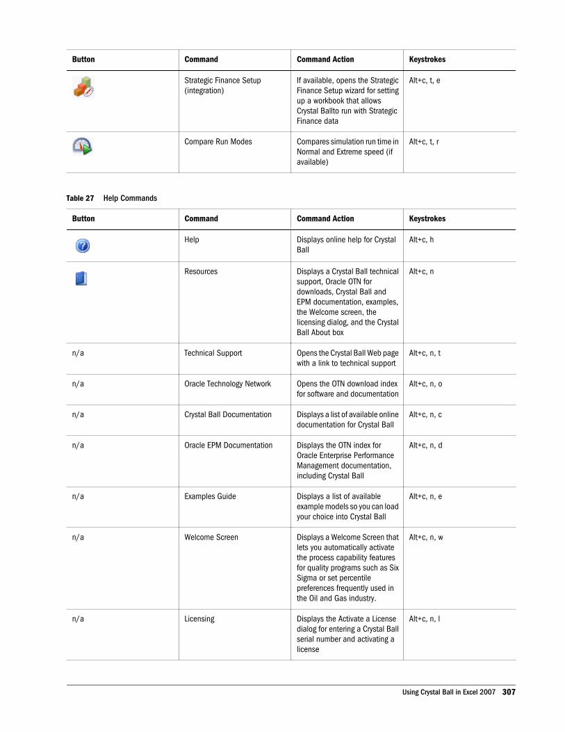
Button Command Command Action Keystrokes
Strategic Finance Setup(integration)
If available, opens the StrategicFinance Setup wizard for settingup a workbook that allowsCrystal Ballto run with StrategicFinance data
Alt+c, t, e
Compare Run Modes Compares simulation run time inNormal and Extreme speed (ifavailable)
Alt+c, t, r
Table 27 Help Commands
Button Command Command Action Keystrokes
Help Displays online help for CrystalBall
Alt+c, h
Resources Displays a Crystal Ball technicalsupport, Oracle OTN fordownloads, Crystal Ball andEPM documentation, examples,the Welcome screen, thelicensing dialog, and the CrystalBall About box
Alt+c, n
n/a Technical Support Opens the Crystal Ball Web pagewith a link to technical support
Alt+c, n, t
n/a Oracle Technology Network Opens the OTN download indexfor software and documentation
Alt+c, n, o
n/a Crystal Ball Documentation Displays a list of available onlinedocumentation for Crystal Ball
Alt+c, n, c
n/a Oracle EPM Documentation Displays the OTN index forOracle Enterprise PerformanceManagement documentation,including Crystal Ball
Alt+c, n, d
n/a Examples Guide Displays a list of availableexample models so you can loadyour choice into Crystal Ball
Alt+c, n, e
n/a Welcome Screen Displays a Welcome Screen thatlets you automatically activatethe process capability featuresfor quality programs such as SixSigma or set percentilepreferences frequently used inthe Oil and Gas industry.
Alt+c, n, w
n/a Licensing Displays the Activate a Licensedialog for entering a Crystal Ballserial number and activating alicense
Alt+c, n, l
Using Crystal Ball in Excel 2007 307
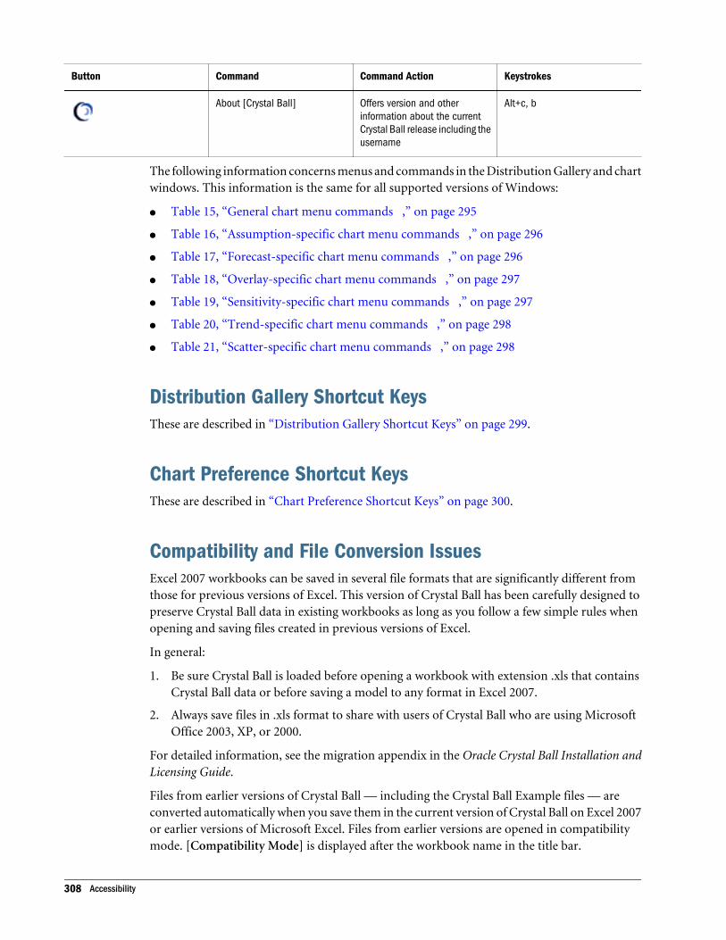
Button Command Command Action Keystrokes
About [Crystal Ball] Offers version and otherinformation about the currentCrystal Ball release including theusername
Alt+c, b
The following information concerns menus and commands in the Distribution Gallery and chartwindows. This information is the same for all supported versions of Windows:
l Table 15, “General chart menu commands ,” on page 295
l Table 16, “Assumption-specific chart menu commands ,” on page 296
l Table 17, “Forecast-specific chart menu commands ,” on page 296
l Table 18, “Overlay-specific chart menu commands ,” on page 297
l Table 19, “Sensitivity-specific chart menu commands ,” on page 297
l Table 20, “Trend-specific chart menu commands ,” on page 298
l Table 21, “Scatter-specific chart menu commands ,” on page 298
Distribution Gallery Shortcut KeysThese are described in “Distribution Gallery Shortcut Keys” on page 299.
Chart Preference Shortcut KeysThese are described in “Chart Preference Shortcut Keys” on page 300.
Compatibility and File Conversion IssuesExcel 2007 workbooks can be saved in several file formats that are significantly different fromthose for previous versions of Excel. This version of Crystal Ball has been carefully designed topreserve Crystal Ball data in existing workbooks as long as you follow a few simple rules whenopening and saving files created in previous versions of Excel.
In general:
1. Be sure Crystal Ball is loaded before opening a workbook with extension .xls that containsCrystal Ball data or before saving a model to any format in Excel 2007.
2. Always save files in .xls format to share with users of Crystal Ball who are using MicrosoftOffice 2003, XP, or 2000.
For detailed information, see the migration appendix in the Oracle Crystal Ball Installation andLicensing Guide.
Files from earlier versions of Crystal Ball — including the Crystal Ball Example files — areconverted automatically when you save them in the current version of Crystal Ball on Excel 2007or earlier versions of Microsoft Excel. Files from earlier versions are opened in compatibilitymode. [Compatibility Mode] is displayed after the workbook name in the title bar.
308 Accessibility

Note: When you open the Example files in Windows Vista, they are read-only. To edit orcustomize them, save them under another name before you run a simulation.
Using Crystal Ball in Excel 2007 309

310 Accessibility
CUsing the Extreme Speed Feature
In This Appendix
Overview ... . . . . . . . . . . . . . . . . . . . . . . . . . . . . . . . . . . . . . . . . . . . . . . . . . . . . . . . . . . . . . . . . . . . . . . . . . . . . . . . . . . . . . . . . . . . . . . . . . . . . . . . . . . . . . . . . . . . . . . . 311
Compatibility Issues ... . . . . . . . . . . . . . . . . . . . . . . . . . . . . . . . . . . . . . . . . . . . . . . . . . . . . . . . . . . . . . . . . . . . . . . . . . . . . . . . . . . . . . . . . . . . . . . . . . . . . . . . . . . 312
Numerical Differences and the Compare Run Modes Tool.. . . . . . . . . . . . . . . . . . . . . . . . . . . . . . . . . . . . . . . . . . . . . . . . . . . . . . . . . . . . . . . . . . 318
Other Important Differences ... . . . . . . . . . . . . . . . . . . . . . . . . . . . . . . . . . . . . . . . . . . . . . . . . . . . . . . . . . . . . . . . . . . . . . . . . . . . . . . . . . . . . . . . . . . . . . . . . . 319
Maximizing the Benefits of Extreme Speed ... . . . . . . . . . . . . . . . . . . . . . . . . . . . . . . . . . . . . . . . . . . . . . . . . . . . . . . . . . . . . . . . . . . . . . . . . . . . . . . . . . 321
OverviewExtreme speed, available in Crystal Ball Decision Optimizer, runs simulations up to 100 timesfaster than Normal speed. With Extreme speed, you won’t need to wait for simulation results orcompromise on the number of trials you run. Extreme speed makes it more practical to useCrystal Ball tools that run multi-simulations or to seek optimal solutions with OptQuest in areasonable length of time.
The Extreme Speed feature uses PSI Technology, a high-speed, Excel-compatible PolymorphicSpreadsheet Interpreter for running simulations on workbooks. This technology was developedby Frontline Systems, the maker of Excel’s Solver add-in. PSI Technology supports nearly all ofthe 320 standard Excel functions, including the financial, statistical, and engineering functionsthat are part of the Analysis Toolpak.
By default, Crystal Ball Decision Optimizer is set to use Extreme speed when initially loaded. Ifa model is not compatible with Extreme speed, a dialog offers the opportunity to downshift toNormal speed temporarily for that simulation. “Compatibility Issues” on page 312 below,explains conditions that cause a model to be incompatible with Extreme speed. The simulationspeed can be changed using the Speed tab in the Run Preferences dialogs (see “Setting SpeedPreferences” on page 78 for details).
This section contains the following main topics:
l “Compatibility Issues” on page 312
l “Numerical Differences and the Compare Run Modes Tool” on page 318
l “Other Important Differences” on page 319
l “Maximizing the Benefits of Extreme Speed” on page 321
Overview 311
Note: Because the Extreme Speed feature uses the Polymorphic Spreadsheet Interpreter, certainExtreme Speed functions may return slightly different results than the correspondingExcel function for extreme values of any input arguments. For example, this can occurwith statistical and inverse distribution functions.
Compatibility IssuesWhile Extreme speed can greatly decrease simulation run times, not all models are compatiblewith Extreme speed. When you start a simulation, Crystal Ball detects if your spreadsheet iscompatible with Extreme speed and warns you if it is incompatible. If you choose, you can runthe simulation in Normal speed using standard Excel, or you can change your spreadsheet modelto correct the incompatibility.
This section lists functions and formula constructs that are not compatible with Extreme speedand suggests workarounds. Besides the issues listed below, some differences may also exist dueto undocumented Excel behaviors, changes in the newest versions of Excel, and so on. Also,small differences in the last few decimal places of certain built-in function values should beexpected, due to minor algorithmic differences in the way formulas might be computed.
It is important to note that incompatibilities in functions and formula constructs only concernthe cells involved in the calculation of a forecast cell. If there are incompatibilities in cells thatare not part of that calculation path, these are not detected and the simulation is allowed to run.
This section discusses the following compatibility issues:
l “Multiple-Workbook Models” on page 312
l “Circular References” on page 313
l “Crystal Ball Excel Functions” on page 313
l “User-Defined Functions” on page 314
l “Running User-Defined Macros” on page 316
l “Special Functions” on page 316
l “Undocumented Behavior of Standard Functions” on page 316
l “Incompatible Range Constructs” on page 316
l “Data Tables” on page 318
Multiple-Workbook ModelsExtreme speed can now run simulations on multiple workbooks. If you are running in Extremespeed and the workbook contains external references to cells in other closed workbooks, CrystalBall obtains the current value from those workbooks. References to cells in other openworkbooks are dynamically updated if those cells depend on one or more assumptions. If theexternal reference is part of a formula (not a simple external reference), this is not compatiblewith Extreme speed:
312 Using the Extreme Speed Feature
l Example message: "Unable to interpret formula at cell location [Book1.xls]Sheet1!A1. (Code#5524 - Complex external reference)"
l Workaround: If possible, consolidate all of the variables and formulas from a multi-workbook model containing Crystal Ball data into a single workbook.
Circular ReferencesCircular references within a model are supported as long as Iteration is checked on the Tools,then Options, then Calculation tab in Excel.
(In Excel 2007, click the Office button and choose Excel Options, then Formulas, and then checkEnable Iterative Calculation in the Calculation Options group.)
If Crystal Ball detects a circular reference and Iteration is not checked, this error is displayed:
l Example message: "Circular reference detected at cell [Book1.xls]Sheet1!A1. (Code #5523)"
l Workaround: Stop the simulation and check Iteration on the Tools, then Options, thenCalculation tab.
In Extreme speed, circular references with short Iteration setting may not match Excel’svalues because of differences in calculation algorithms. For most consistent results, setIteration to at least 1,000.
However, if a circular reference is non-converging, its results can differ greatly when run at bothExtreme and Normal speed, regardless of the Iteration setting. If a circular reference is non-converging, this error message is displayed:
l Example message: "Unable to run in Extreme speed for the following reason: Circularreferences do not converge, results cannot be guaranteed to match Normal speed. To bypassthis message, turn off "Stop on calculation errors" in the Run Preferences dialog. (Code#5545)"
l Workaround: There is no workaround. Check the formulas in the workbook that havecreated this circular reference and look for a problem that keeps this circular reference fromconverging to a single value.
Simulations with circular references run in non-vectorized mode. For this reason, they willprobably run more slowly than simulations without circular references.
Crystal Ball Excel FunctionsThe following Crystal Ball spreadsheet functions are handled normally:
l CB.IterationsFN
l distribution functions (such as CB.Binomial)
These functions are not supported in Extreme speed during a simulation:
l CB.GetForeStatFN
l CB.GetForePercentFN
Compatibility Issues 313
l CB.GetRunPrefsFN
l CB.GetAssumPercentFN
l CB.GetCertaintyFN
While running in Extreme speed, all values for these functions return #VALUE. At the end ofthe simulation, Crystal Ball performs a final recalculation on the model so these functions areevaluated properly. Normally, this should not present a problem unless one of these functionswas defined as a forecast and you are expecting a valid value to be computed during thesimulation. If one of these "Get" functions feeds into a forecast during a simulation, this is notcompatible with Extreme speed:
l Example message: "Unsupported Excel or Crystal Ball function at cell location[Book1.xls]Sheet1!A1. (Code #5539)"
l Workaround: Defining forecasts on statistical functions that are dependent on otherforecasts is generally not a good modeling practice. If you need to have a forecast cell definedon a statistical result from another forecast, use the Auto Extract feature for the dependentforecast instead of using one of the above Crystal Ball functions.
User-Defined FunctionsCalls to user-defined or third-party functions are allowed. The functions may be written in VisualBasic or they may be in XLL or COM Automation DLL libraries that have been opened in Excel.
This section includes the following topics:
l “Pure Functions” on page 314
l “Range Arguments” on page 314
l “Volatile Functions and Array Arguments” on page 315
Pure FunctionsTo be compatible with Extreme Speed, user-defined functions must be "pure." A "pure function"is one that computes its value solely on the basis of values passed to it as arguments. A functionthat is not "pure" might reference global data not passed as an argument. For example, it mightget the value of a worksheet cell or a defined name and use this as an input to compute thefunction value. If the global data depends on the assumptions — if, for example, it is a worksheetcell with a formula computed from the assumptions — it will have a distribution of values inNormal Speed, but it will appear deterministic (have a single value) in Extreme Speed. This isbecause the worksheet cells change on every trial in Normal Speed, but they do not change inExtreme Speed.
Range ArgumentsRange arguments in user-defined functions are only compatible with Extreme Speed when theyare handled as Variant types. For example, for a function called on the worksheet as=MyFunc(A1:E4, 5, 4):
314 Using the Extreme Speed Feature
Function MyFunc (MyData As Variant, Rows As Long, Cols As Long) As Double For I = 1 to Rows For J = 1 to Cols MsgBox MyData(I, J) 'or otherwise work with the cell range as an array Next J Next IEnd Function
Volatile Functions and Array ArgumentsUser-defined functions whose arguments are static (their values do not change during asimulation) are not called by Extreme Speed unless the Volatile property of the function hasbeen set.
When a user-defined function is encountered in Extreme Speed, Crystal Ball first checks to seeif the function is Volatile. If Crystal Ball is denied access to the VBA project and the user-definedfunction is not passing array or cell range arguments, Crystal Ball treats the function as Volatile.
If access to the project is denied and the call is passing array or cell range arguments, the followingmessage is displayed:
Cannot interpret a user-defined function with array arguments. You must first check the ‘TrustAccess to Visual Basic Project’ checkbox in Excel’s macro security settings dialog. See AppendixC in the User's Guide for more information about this error.
Cause: The Excel Volatile property has not been set.
ä In that case, in order for Extreme Speed to determine the state of the Volatile property in Excel2002 (XP) and later, you must first make the following setting in Excel:
1 Go to the Tools, then Options panel.
2 Click the Security tab.
3 Click the Macro Security button.
4 Click the Trusted Publishers tab.
5 Check Trust Access To Visual Basic Project.
In Excel 2007, you should not encounter this specific problem with array arguments or anyothers involving the Analysis ToolPak, since the ToolPak is embedded directly into Excel 2007.
ä However, to set the "Trust access..." property in Excel 2007 to ensure that the Volatile propertyis set correctly, follow these steps:
1 Click the Office button.
2 Click the following sequence of buttons and links: Excel Options, then Trust Center, then Trust Center Settings,then Macro Settings.
3 On the Macro Settings page, under Developer Macro Settings, check "Trust access to the VBA project objectmodel."
Note that all user-defined functions are treated as Volatile in Excel 2000.
Compatibility Issues 315
Running User-Defined MacrosIn Extreme speed, it is not possible to run user-defined macros — such as CBBeforeTrial,CBAfterTrial, and CBAfterRecalc — during a simulation. Before- and after-simulation macrosare allowed, such as CBBeforeSimulation and CBAfterSimulation. If the former group ofsimulation macros are present, they will be flagged as incompatible:
l Example message: "One or more user-defined simulation macros were detected (e.g.,CBBeforeTrial, CBAfterTrial, etc.). (Code #5701)"
l Workaround: Use Normal speed to run these user-defined macros during a simulation.
Special FunctionsA small group of Excel functions are not supported in Extreme speed: CALL, CELL,GETPIVOTDATA, INFO, HYPERLINK, REGISTER.ID, and the CUBE functions added in Excel2007 (CUBEMEMBER, CUBEVALUE, CUBESET, CUBESETCOUNT,CUBERANKEDMEMBER, CUBEMEMBERPROPERTY, CUBEKPIMEMBER) . OFFSET hasalso been reported as incompatible. Any forecast formulas that contain one or more of thesefunctions will be flagged as incompatible:
l Example message: "Unsupported Excel or Crystal Ball function at cell location[Book1.xls]Sheet1!A1. (Code #5539)
l Workaround: Avoid using these functions if you want to run the model in Extreme speed.
Undocumented Behavior of Standard FunctionsExcel allows certain undocumented argument constructs for standard functions. Some of theseconstructs that were previously unsupported in Extreme speed are now allowed, for example:
=SUMPRODUCT(A1:A10*B1:B10)=SUMPRODUCT(A1:A10/B1:B10)
However, some of these argument constructs are still not supported in Extreme speed and willbe flagged as incompatible:
l Example message: "Unsupported Excel or Crystal Ball function at cell location[Book1.xls]Sheet1!A1. (Code #5539)"
l Workaround: For best results, always use standard syntax with fully valid arguments.
Incompatible Range ConstructsThe following sections discuss Excel range constructs that are not supported in Extreme speed:
l “Dynamic Ranges” on page 317
l “Labels in Formulas That Are Not Defined Names” on page 317
l “Multiple Area References” on page 317
l “3-D References” on page 317
316 Using the Extreme Speed Feature
Dynamic RangesExtreme speed does not support dynamic ranges, where the OFFSET function is used on one orboth sides of the range ":" constructor. For example,=AVERAGE(Cellname1:OFFSET(Cellname2, x, y)).
l Example message: "Unable to interpret formula at cell location [Book1.xls]Sheet1!A1. (Code#5504 - Invalid token)"
l Workaround: Avoid using the OFFSET function to construct dynamic ranges.
Labels in Formulas That Are Not Defined NamesExtreme speed supports defined names and their use in formulas, but not the Excel "Acceptlabels in formulas" option which allows cell labels to be used in formulas without defining themas names:
l Example message: "Unable to interpret formula at cell location [Book1.xls]Sheet1!A1. (Code#5514 - Undefined identifier)"
l Workaround: For best results, use defined names instead of cell labels in formulas.
Multiple Area ReferencesExtreme speed does not support multiple-area references such as (A1:A5,B1,C1:E1) except asused in standard functions such as SUM that accept a variable-length argument list of cell ranges.The only supported use of the comma is as the separator in the argument list of a standardfunction, not as a cell-range "union operator." A defined name whose value is a multiple-areareference is not accepted:
l Example message: "Multi-area reference not supported at cell location [Book1.xls]Sheet1!A1. (Code #5525)"
l Workaround: For best results, avoid using multiple-area references when defining namesor as arguments to any functions except those that accept a variable-length, comma-separated list of cell ranges.
3-D ReferencesExtreme speed does not support 3-D references, where a cell range – used as an argument in afunction call, for example – spans multiple workbooks:
l Example message: "Unable to interpret formula at cell location [Book1.xls]Sheet1!A1.("Code #5514 - Undefined identifier")
l Workaround: For best results, avoid using 3-D cell references.
Compatibility Issues 317
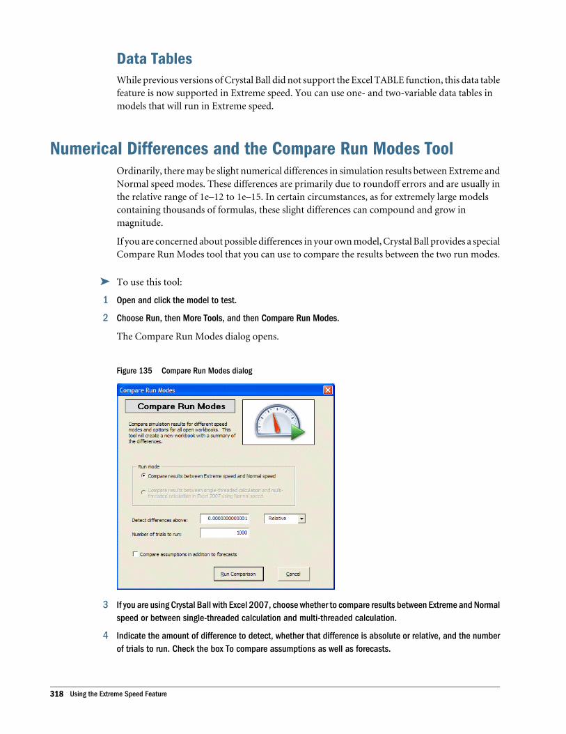
Data TablesWhile previous versions of Crystal Ball did not support the Excel TABLE function, this data tablefeature is now supported in Extreme speed. You can use one- and two-variable data tables inmodels that will run in Extreme speed.
Numerical Differences and the Compare Run Modes ToolOrdinarily, there may be slight numerical differences in simulation results between Extreme andNormal speed modes. These differences are primarily due to roundoff errors and are usually inthe relative range of 1e–12 to 1e–15. In certain circumstances, as for extremely large modelscontaining thousands of formulas, these slight differences can compound and grow inmagnitude.
If you are concerned about possible differences in your own model, Crystal Ball provides a specialCompare Run Modes tool that you can use to compare the results between the two run modes.
ä To use this tool:
1 Open and click the model to test.
2 Choose Run, then More Tools, and then Compare Run Modes.
The Compare Run Modes dialog opens.
Figure 135 Compare Run Modes dialog
3 If you are using Crystal Ball with Excel 2007, choose whether to compare results between Extreme and Normalspeed or between single-threaded calculation and multi-threaded calculation.
4 Indicate the amount of difference to detect, whether that difference is absolute or relative, and the numberof trials to run. Check the box To compare assumptions as well as forecasts.
318 Using the Extreme Speed Feature

Depending on the size of your model, differences might not become obvious until after a fairlylarge number of trials have run. You might want to run 5,000 or more trials for your test.
5 When you are ready, click Run Comparison.
If you are comparing speed results, the simulation runs once in Extreme speed and once inNormal speed. Otherwise, the simulation runs once with single-threaded and once with multi-threaded calculations. Results are displayed in a new workbook. The comparison Summary tabis displayed when the comparison is complete.
Figure 136 shows comparison results for the Tolerance Analysis.xls example file with 5,000 trials.In this case there were no differences in results and the model ran 28.8 times faster in Extremespeed.
Figure 136 Comparison results for Tolerance Analysis.xls, 5,000 trials
Because of variations in the random number seeds, you might see differences in comparisionresults if you use Excel’s RAND or Crystal Ball’s probability functions (such as CB.Uniform) inyour model.
Other Important DifferencesThis section discusses several other differences between Extreme speed and Normal speed:
l “OptQuest and other Crystal Ball Tools” on page 320
Other Important Differences 319
l “Precision Control and Cell Error Checking” on page 320
l “Spreadsheet Updating” on page 320
l “Very Large Models” on page 320
l “Memory Usage” on page 321
l “Spreadsheets with No Crystal Ball Data” on page 321
OptQuest and other Crystal Ball ToolsOptQuest and certain other Crystal Ball tools run multiple simulations of your spreadsheetmodel back-to-back. Since Extreme speed enhances the performance of each simulation, youwill see an overall speed improvement when using one of these tools. All of the compatibilityand other differences apply to these tools as well.
Precision Control and Cell Error CheckingExtreme speed uses a bursting feature to optimize the balance between speed and systemresponsiveness. Since bursts are usually several hundreds or thousands of trials at a time, thisfeature affects a number of features like precision control, confidence testing, and checking forcell errors.
Crystal Ball tests for precision control (and performs confidence testing in OptQuest) after eachburst of several hundred or thousands of trials. In Normal speed, these checks are performedevery 50 trials by default. As a result, you may see your simulations run more trials than usualwhen these features are turned on. Generally speaking, these features are not as critical tosimulation performance in Extreme speed as they are in Normal speed.
Because of bursting, Crystal Ball cannot check cell errors after every trial as it does in Normalspeed, only at the end of a burst. If cell errors occur in forecast cells (such as "Divide by zero" or"#VALUE") and the Run Preferences, then Stop On Calculation Errors option is selected, thesimulation stops at the end of the next burst.
Spreadsheet UpdatingWhile running simulations in Extreme speed, cells in your spreadsheet model appear to updateevery second or so after each burst. This is normal and does not affect simulation results. Single-stepping mode still updates cell values for every step.
Very Large ModelsVery large models (with greater than 10,000 formulas, for example), might take Crystal Ballmany seconds or minutes in Extreme speed to analyze the model and convert it into a form forhigh-speed simulation. When this happens, the following progress dialog opens.
320 Using the Extreme Speed Feature

Figure 137 Extreme Speed Progress Dialog Box
If you choose, you can cancel the simulation by pressing the Ctrl+Break keys or wait for theprocess to finish.
Memory UsageRunning simulations in Extreme speed is extremely memory-intensive. Depending on yourmachine, you may encounter issues with memory usage when running long simulations orworking with large models.
During a long simulation (greater than 100,000 trials), you might also see that your machine’svirtual memory is being used. For example, you might notice that your hard drive is beingaccessed continually and the simulation starts to slow down. No message is given when thiscondition occurs. If such a slow-down occurs and it is absolutely necessary that additional trialsbe run, you can try to disable the saving of assumption values (see the Run Preferences, thenOptions tab) and then restart the simulation.
If you run an Extreme Speed simulation multiple times on a large or complex model, you mightfind that you receive the "Sufficient memory may not..." warning dialog. This dialog lets youdisable the Store Assumption Values run preference and change the number of trials to run.Notice that these changes in the warning dialog reset those preferences in the Run Preferencesdialog on the Trials and Options tabs. They are then applied to other models unless you resetthem after the large model has run.
Spreadsheets with No Crystal Ball DataSpreadsheets without Crystal Ball data always run in Normal speed even if Extreme speed isselected in the Run Preferences dialog.
This could happen if you have Crystal Ball spreadsheet functions entered in the model but havenot defined assumptions, forecasts, or decision variables.
Maximizing the Benefits of Extreme SpeedTo get maximum benefit from running Crystal Ball in Extreme speed, you should be aware ofseveral issues in your models that could potentially cause simulations to run more slowly thanexpected.
When you first start a simulation in Extreme speed, the model is analyzed and converted into aspecial form for high-speed processing. This form involves the use of a technique calledvectorization to process batches of formula results together for maximum efficiency. Certain
Maximizing the Benefits of Extreme Speed 321
functions and formula constructs in your model can interfere with this vectorization process.Some of the more common cases are discussed in the following sections:
l “String Intermediate Results in Formulas” on page 322
l “Calls to User-Defined Functions” on page 322
l “Dynamic Assumptions” on page 322
l “Excel Functions” on page 323
If one or more cases are detected, Crystal Ball Decision Optimizer displays the message "non-vectored" on the Excel status bar while the simulation is running. Also, additional informationis usually written to the Crystal Ball log file, which can be found with the suffix CB Log andextension .txt in:
C:\Documents and Settings\username\Application Data\Oracle\ Crystal Ball\11.0\Logs\CB Log_x.txt
Note: If you have a very large number of trials, the virtual memory feature of Microsoft Windowsis activated. This can slow down processing. Too, if you have large numbers of forecastsand assumptions, managing these large arrays of values can take extra time. If you thinkarray management could be an issue, try unchecking Store Assumption Values ForSensitivity Analysis on the Options tab of the Run Preferences dialog.
String Intermediate Results in FormulasIn Excel, it is possible to construct formulas that produce an intermediate character string result,which is used in later formulas to produce a numeric result. For maximum speed gains, youshould avoid the use of strings in your formulas. Strings in formulas will not be flagged asincompatible, but will cause simulations to run much slower depending on the number of stringformulas in your model.
l Workaround: Some simple strings like "Yes" and "No" can be replaced with 1 and 0 values,or True and False Boolean values.
Calls to User-Defined FunctionsCalls to user-defined or third-party functions cannot be vectorized and will cause simulationsto run slower.
l Workaround: There is no workaround for this case other than minimizing the use of thesefunctions.
Dynamic AssumptionsAssumptions that contain cell references to parameter values that can change during a simulationare called dynamic assumptions. Crystal Ball needs to perform additional validation checks onthe parameters for these assumption types during a simulation, causing simulations to run moreslowly.
322 Using the Extreme Speed Feature
l Workaround: If the dynamic assumption feature is not needed, make sure that parametercell references do not point to other assumption cells in your model.
Cell references in custom distributions are treated as static instead of dynamic when a model isrun at Extreme speed.
Excel FunctionsCrystal Ball supports LOOKUP and OFFSET functions in both Normal and Extreme speed.However, if you use more than a thousand in a model, this can slow down the initial parsingtime and cause the simulation to run slowly.
Maximizing the Benefits of Extreme Speed 323

324 Using the Extreme Speed Feature
DCrystal Ball Tutorials
In This Appendix
Introduction... . . . . . . . . . . . . . . . . . . . . . . . . . . . . . . . . . . . . . . . . . . . . . . . . . . . . . . . . . . . . . . . . . . . . . . . . . . . . . . . . . . . . . . . . . . . . . . . . . . . . . . . . . . . . . . . . . . . . 325
Tutorial 1 — Futura Apartments ... . . . . . . . . . . . . . . . . . . . . . . . . . . . . . . . . . . . . . . . . . . . . . . . . . . . . . . . . . . . . . . . . . . . . . . . . . . . . . . . . . . . . . . . . . . . . . . 325
Tutorial 2 — Vision Research... . . . . . . . . . . . . . . . . . . . . . . . . . . . . . . . . . . . . . . . . . . . . . . . . . . . . . . . . . . . . . . . . . . . . . . . . . . . . . . . . . . . . . . . . . . . . . . . . . 333
Improving Process Quality — Tutorial 3 ... . . . . . . . . . . . . . . . . . . . . . . . . . . . . . . . . . . . . . . . . . . . . . . . . . . . . . . . . . . . . . . . . . . . . . . . . . . . . . . . . . . . . . 352
Packaging Pump Design — Tutorial 4 ... . . . . . . . . . . . . . . . . . . . . . . . . . . . . . . . . . . . . . . . . . . . . . . . . . . . . . . . . . . . . . . . . . . . . . . . . . . . . . . . . . . . . . . . 366
IntroductionThis appendix presents the basics you need to understand how Crystal Ball can be used to analyzeuncertainty in two financial settings, a process improvement setting, and a product designsetting.
l “Tutorial 1 — Futura Apartments” on page 325 is ready to run so you can quickly see howCrystal Ball works. If you work regularly with statistics and forecasting techniques, this mightbe all the introduction you need before running your own spreadsheets with Crystal Ball.
l “Tutorial 2 — Vision Research” on page 333 teaches more about defining and runningsimulations and interpreting their results.
l “Improving Process Quality — Tutorial 3” on page 352 shows howCrystal Ball supportsprocess improvement initiatives similar to Six Sigma.
l “Packaging Pump Design — Tutorial 4” on page 366 shows how Crystal Ball supportsquality initiatives for product and system design, such as Design for Six Sigma (DFSS).
Tutorial 1 — Futura ApartmentsThis tutorial contains the following sections::
l “Starting Crystal Ball” on page 326
l “Opening the Example Model” on page 327
l “Running Simulations” on page 328
l “Results Analysis — Determining Profit” on page 329
l “Take a Look Behind the Scenes” on page 330
l “Resetting and Single-Stepping” on page 331
Introduction 325
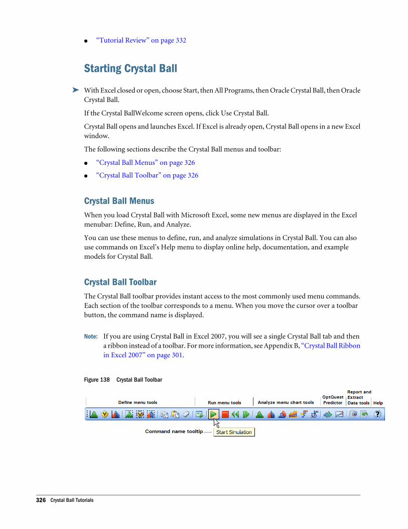
l “Tutorial Review” on page 332
Starting Crystal Ball
ä With Excel closed or open, choose Start, then All Programs, then Oracle Crystal Ball, then OracleCrystal Ball.
If the Crystal BallWelcome screen opens, click Use Crystal Ball.
Crystal Ball opens and launches Excel. If Excel is already open, Crystal Ball opens in a new Excelwindow.
The following sections describe the Crystal Ball menus and toolbar:
l “Crystal Ball Menus” on page 326
l “Crystal Ball Toolbar” on page 326
Crystal Ball MenusWhen you load Crystal Ball with Microsoft Excel, some new menus are displayed in the Excelmenubar: Define, Run, and Analyze.
You can use these menus to define, run, and analyze simulations in Crystal Ball. You can alsouse commands on Excel’s Help menu to display online help, documentation, and examplemodels for Crystal Ball.
Crystal Ball ToolbarThe Crystal Ball toolbar provides instant access to the most commonly used menu commands.Each section of the toolbar corresponds to a menu. When you move the cursor over a toolbarbutton, the command name is displayed.
Note: If you are using Crystal Ball in Excel 2007, you will see a single Crystal Ball tab and thena ribbon instead of a toolbar. For more information, see Appendix B, “Crystal Ball Ribbonin Excel 2007” on page 301.
Figure 138 Crystal Ball Toolbar
326 Crystal Ball Tutorials
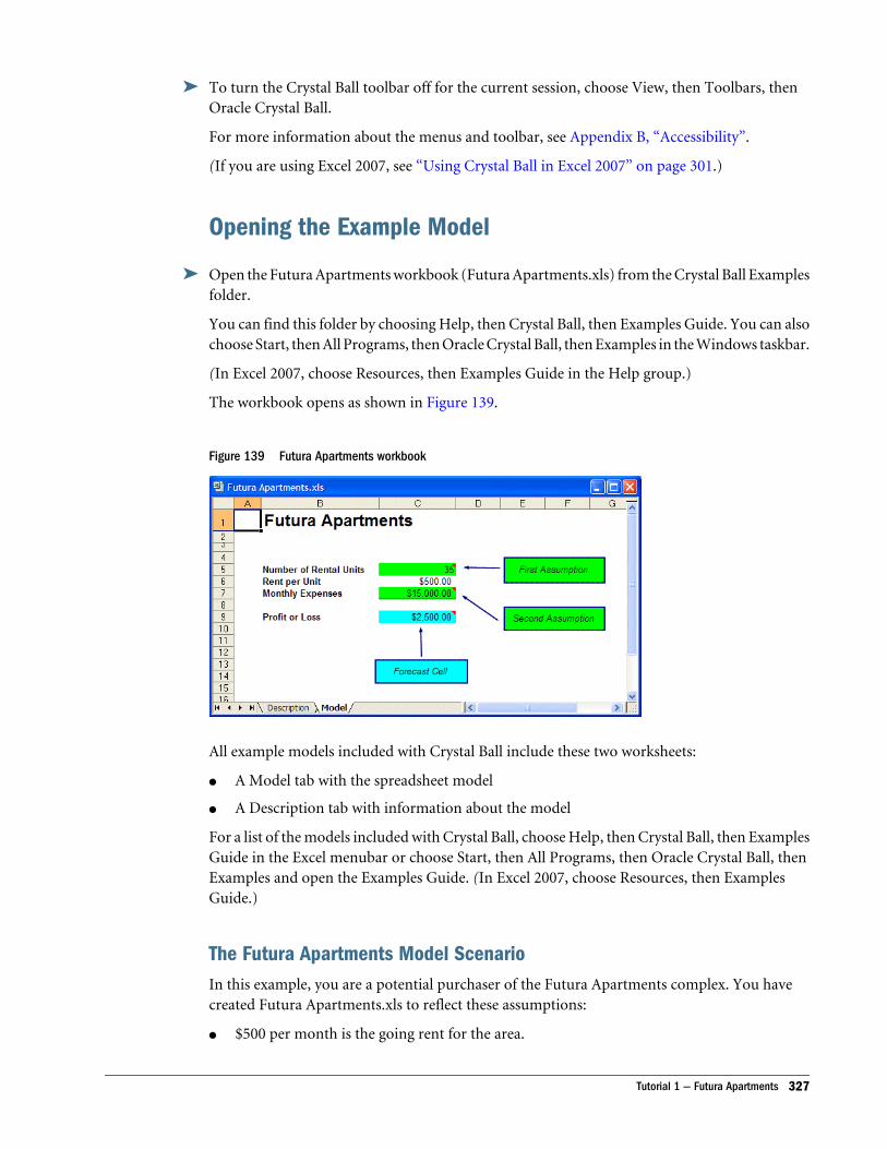
ä To turn the Crystal Ball toolbar off for the current session, choose View, then Toolbars, thenOracle Crystal Ball.
For more information about the menus and toolbar, see Appendix B, “Accessibility”.
(If you are using Excel 2007, see “Using Crystal Ball in Excel 2007” on page 301.)
Opening the Example Model
ä Open the Futura Apartments workbook (Futura Apartments.xls) from the Crystal Ball Examplesfolder.
You can find this folder by choosing Help, then Crystal Ball, then Examples Guide. You can alsochoose Start, then All Programs, then Oracle Crystal Ball, then Examples in the Windows taskbar.
(In Excel 2007, choose Resources, then Examples Guide in the Help group.)
The workbook opens as shown in Figure 139.
Figure 139 Futura Apartments workbook
All example models included with Crystal Ball include these two worksheets:
l A Model tab with the spreadsheet model
l A Description tab with information about the model
For a list of the models included with Crystal Ball, choose Help, then Crystal Ball, then ExamplesGuide in the Excel menubar or choose Start, then All Programs, then Oracle Crystal Ball, thenExamples and open the Examples Guide. (In Excel 2007, choose Resources, then ExamplesGuide.)
The Futura Apartments Model ScenarioIn this example, you are a potential purchaser of the Futura Apartments complex. You havecreated Futura Apartments.xls to reflect these assumptions:
l $500 per month is the going rent for the area.
Tutorial 1 — Futura Apartments 327
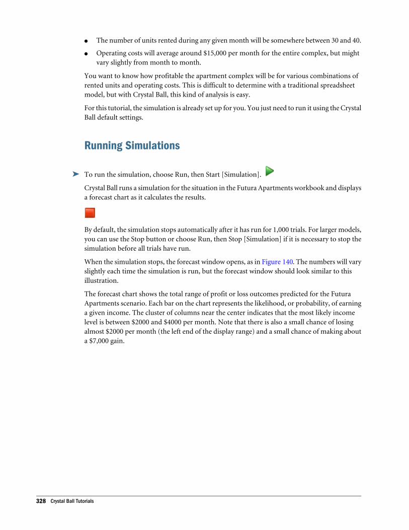
l The number of units rented during any given month will be somewhere between 30 and 40.
l Operating costs will average around $15,000 per month for the entire complex, but mightvary slightly from month to month.
You want to know how profitable the apartment complex will be for various combinations ofrented units and operating costs. This is difficult to determine with a traditional spreadsheetmodel, but with Crystal Ball, this kind of analysis is easy.
For this tutorial, the simulation is already set up for you. You just need to run it using the CrystalBall default settings.
Running Simulations
ä To run the simulation, choose Run, then Start [Simulation].
Crystal Ball runs a simulation for the situation in the Futura Apartments workbook and displaysa forecast chart as it calculates the results.
By default, the simulation stops automatically after it has run for 1,000 trials. For larger models,you can use the Stop button or choose Run, then Stop [Simulation] if it is necessary to stop thesimulation before all trials have run.
When the simulation stops, the forecast window opens, as in Figure 140. The numbers will varyslightly each time the simulation is run, but the forecast window should look similar to thisillustration.
The forecast chart shows the total range of profit or loss outcomes predicted for the FuturaApartments scenario. Each bar on the chart represents the likelihood, or probability, of earninga given income. The cluster of columns near the center indicates that the most likely incomelevel is between $2000 and $4000 per month. Note that there is also a small chance of losingalmost $2000 per month (the left end of the display range) and a small chance of making abouta $7,000 gain.
328 Crystal Ball Tutorials
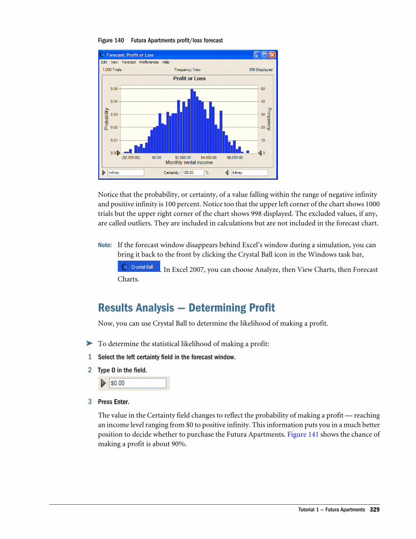
Figure 140 Futura Apartments profit/loss forecast
Notice that the probability, or certainty, of a value falling within the range of negative infinityand positive infinity is 100 percent. Notice too that the upper left corner of the chart shows 1000trials but the upper right corner of the chart shows 998 displayed. The excluded values, if any,are called outliers. They are included in calculations but are not included in the forecast chart.
Note: If the forecast window disappears behind Excel’s window during a simulation, you canbring it back to the front by clicking the Crystal Ball icon in the Windows task bar,
. In Excel 2007, you can choose Analyze, then View Charts, then ForecastCharts.
Results Analysis — Determining ProfitNow, you can use Crystal Ball to determine the likelihood of making a profit.
ä To determine the statistical likelihood of making a profit:
1 Select the left certainty field in the forecast window.
2 Type 0 in the field.
3 Press Enter.
The value in the Certainty field changes to reflect the probability of making a profit — reachingan income level ranging from $0 to positive infinity. This information puts you in a much betterposition to decide whether to purchase the Futura Apartments. Figure 141 shows the chance ofmaking a profit is about 90%.
Tutorial 1 — Futura Apartments 329
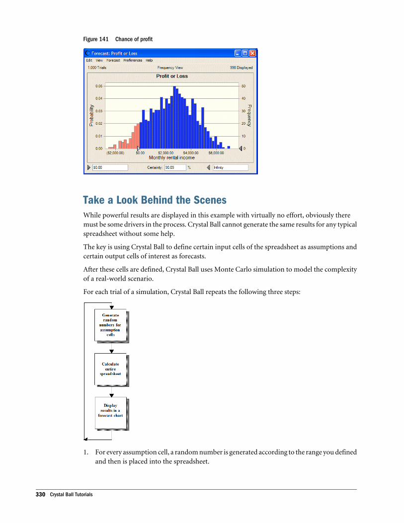
Figure 141 Chance of profit
Take a Look Behind the ScenesWhile powerful results are displayed in this example with virtually no effort, obviously theremust be some drivers in the process. Crystal Ball cannot generate the same results for any typicalspreadsheet without some help.
The key is using Crystal Ball to define certain input cells of the spreadsheet as assumptions andcertain output cells of interest as forecasts.
After these cells are defined, Crystal Ball uses Monte Carlo simulation to model the complexityof a real-world scenario.
For each trial of a simulation, Crystal Ball repeats the following three steps:
1. For every assumption cell, a random number is generated according to the range you definedand then is placed into the spreadsheet.
330 Crystal Ball Tutorials
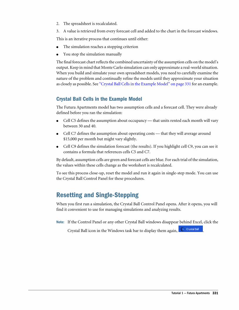
2. The spreadsheet is recalculated.
3. A value is retrieved from every forecast cell and added to the chart in the forecast windows.
This is an iterative process that continues until either:
l The simulation reaches a stopping criterion
l You stop the simulation manually
The final forecast chart reflects the combined uncertainty of the assumption cells on the model’soutput. Keep in mind that Monte Carlo simulation can only approximate a real-world situation.When you build and simulate your own spreadsheet models, you need to carefully examine thenature of the problem and continually refine the models until they approximate your situationas closely as possible. See “Crystal Ball Cells in the Example Model” on page 331 for an example.
Crystal Ball Cells in the Example ModelThe Futura Apartments model has two assumption cells and a forecast cell. They were alreadydefined before you ran the simulation:
l Cell C5 defines the assumption about occupancy — that units rented each month will varybetween 30 and 40.
l Cell C7 defines the assumption about operating costs — that they will average around$15,000 per month but might vary slightly.
l Cell C9 defines the simulation forecast (the results). If you highlight cell C9, you can see itcontains a formula that references cells C5 and C7.
By default, assumption cells are green and forecast cells are blue. For each trial of the simulation,the values within these cells change as the worksheet is recalculated.
To see this process close-up, reset the model and run it again in single-step mode. You can usethe Crystal Ball Control Panel for these procedures.
Resetting and Single-SteppingWhen you first run a simulation, the Crystal Ball Control Panel opens. After it opens, you willfind it convenient to use for managing simulations and analyzing results.
Note: If the Control Panel or any other Crystal Ball windows disappear behind Excel, click the
Crystal Ball icon in the Windows task bar to display them again, .
Tutorial 1 — Futura Apartments 331
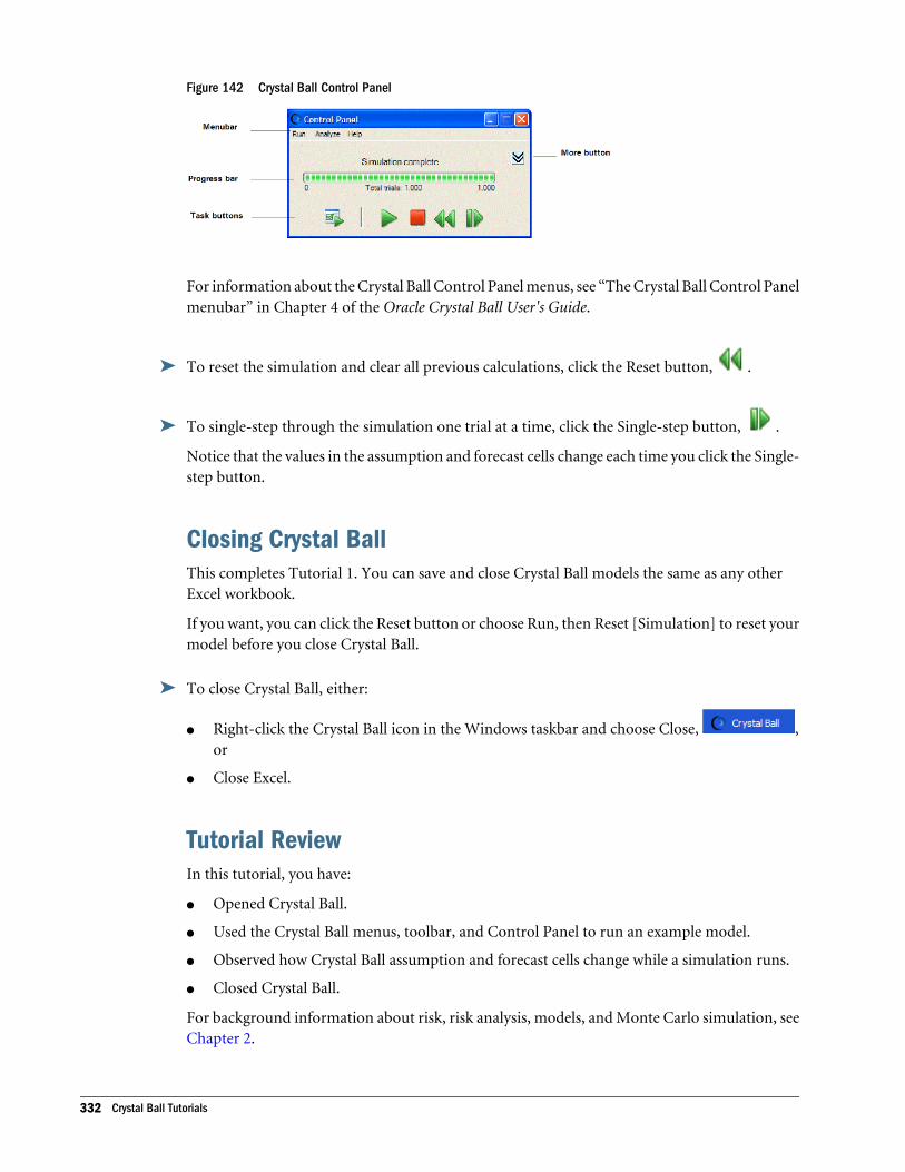
Figure 142 Crystal Ball Control Panel
For information about the Crystal Ball Control Panel menus, see “The Crystal Ball Control Panelmenubar” in Chapter 4 of the Oracle Crystal Ball User's Guide.
ä To reset the simulation and clear all previous calculations, click the Reset button, .
ä To single-step through the simulation one trial at a time, click the Single-step button, .
Notice that the values in the assumption and forecast cells change each time you click the Single-step button.
Closing Crystal BallThis completes Tutorial 1. You can save and close Crystal Ball models the same as any otherExcel workbook.
If you want, you can click the Reset button or choose Run, then Reset [Simulation] to reset yourmodel before you close Crystal Ball.
ä To close Crystal Ball, either:
l Right-click the Crystal Ball icon in the Windows taskbar and choose Close, ,or
l Close Excel.
Tutorial ReviewIn this tutorial, you have:
l Opened Crystal Ball.
l Used the Crystal Ball menus, toolbar, and Control Panel to run an example model.
l Observed how Crystal Ball assumption and forecast cells change while a simulation runs.
l Closed Crystal Ball.
For background information about risk, risk analysis, models, and Monte Carlo simulation, seeChapter 2.
332 Crystal Ball Tutorials
“Tutorial 2 — Vision Research” on page 333, shows how to define assumption and forecast cellsand gives more suggestions for analyzing the results.
Tutorial 2 — Vision ResearchThis tutorial contains the following sections for review and instruction:
l “Starting Crystal Ball” on page 333
l “Opening the Example Model” on page 333
l “Reviewing the Vision Research Scenario” on page 334
l “Defining Assumptions” on page 334
l “Defining Forecasts” on page 344
l “Running Simulations” on page 346
l “Interpreting the Results” on page 347
l “Closing Crystal Ball” on page 352
Starting Crystal BallIf Crystal Ball is not already started, follow the instructions in “Starting Crystal Ball” on page326.
Opening the Example Model
ä Open the Vision Research workbook (Vision Research.xls) from the Crystal Ball Examplesfolder.
You can find this folder by choosing Help, then Crystal Ball, then Examples Guide. You can alsochoose Start, then All Programs, then Oracle Crystal Ball, then Examples in the Windows taskbar.
(In Excel 2007, choose Resources, then Examples Guide.)
The Vision Research workbook for the ClearView project opens, as in Figure 143.
Tutorial 2 — Vision Research 333
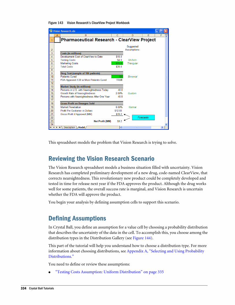
Figure 143 Vision Research’s ClearView Project Workbook
This spreadsheet models the problem that Vision Research is trying to solve.
Reviewing the Vision Research ScenarioThe Vision Research spreadsheet models a business situation filled with uncertainty. VisionResearch has completed preliminary development of a new drug, code-named ClearView, thatcorrects nearsightedness. This revolutionary new product could be completely developed andtested in time for release next year if the FDA approves the product. Although the drug workswell for some patients, the overall success rate is marginal, and Vision Research is uncertainwhether the FDA will approve the product.
You begin your analysis by defining assumption cells to support this scenario.
Defining AssumptionsIn Crystal Ball, you define an assumption for a value cell by choosing a probability distributionthat describes the uncertainty of the data in the cell. To accomplish this, you choose among thedistribution types in the Distribution Gallery (see Figure 144).
This part of the tutorial will help you understand how to choose a distribution type. For moreinformation about choosing distributions, see Appendix A, “Selecting and Using ProbabilityDistributions.”
You need to define or review these assumptions:
l “Testing Costs Assumption: Uniform Distribution” on page 335
334 Crystal Ball Tutorials
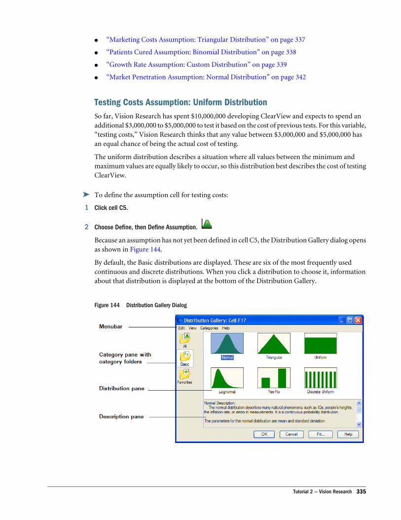
l “Marketing Costs Assumption: Triangular Distribution” on page 337
l “Patients Cured Assumption: Binomial Distribution” on page 338
l “Growth Rate Assumption: Custom Distribution” on page 339
l “Market Penetration Assumption: Normal Distribution” on page 342
Testing Costs Assumption: Uniform DistributionSo far, Vision Research has spent $10,000,000 developing ClearView and expects to spend anadditional $3,000,000 to $5,000,000 to test it based on the cost of previous tests. For this variable,“testing costs,” Vision Research thinks that any value between $3,000,000 and $5,000,000 hasan equal chance of being the actual cost of testing.
The uniform distribution describes a situation where all values between the minimum andmaximum values are equally likely to occur, so this distribution best describes the cost of testingClearView.
ä To define the assumption cell for testing costs:
1 Click cell C5.
2 Choose Define, then Define Assumption.
Because an assumption has not yet been defined in cell C5, the Distribution Gallery dialog opensas shown in Figure 144.
By default, the Basic distributions are displayed. These are six of the most frequently usedcontinuous and discrete distributions. When you click a distribution to choose it, informationabout that distribution is displayed at the bottom of the Distribution Gallery.
Figure 144 Distribution Gallery Dialog
Tutorial 2 — Vision Research 335
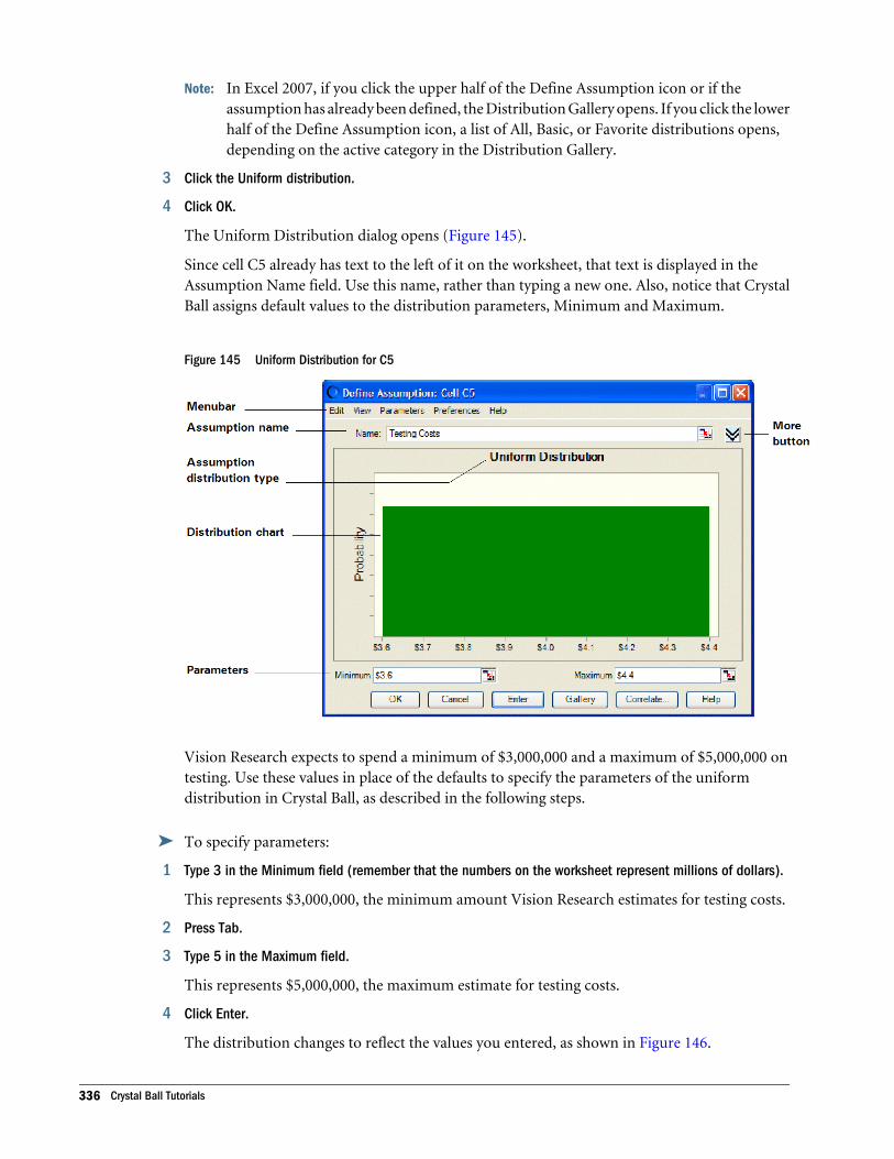
Note: In Excel 2007, if you click the upper half of the Define Assumption icon or if theassumption has already been defined, the Distribution Gallery opens. If you click the lowerhalf of the Define Assumption icon, a list of All, Basic, or Favorite distributions opens,depending on the active category in the Distribution Gallery.
3 Click the Uniform distribution.
4 Click OK.
The Uniform Distribution dialog opens (Figure 145).
Since cell C5 already has text to the left of it on the worksheet, that text is displayed in theAssumption Name field. Use this name, rather than typing a new one. Also, notice that CrystalBall assigns default values to the distribution parameters, Minimum and Maximum.
Figure 145 Uniform Distribution for C5
Vision Research expects to spend a minimum of $3,000,000 and a maximum of $5,000,000 ontesting. Use these values in place of the defaults to specify the parameters of the uniformdistribution in Crystal Ball, as described in the following steps.
ä To specify parameters:
1 Type 3 in the Minimum field (remember that the numbers on the worksheet represent millions of dollars).
This represents $3,000,000, the minimum amount Vision Research estimates for testing costs.
2 Press Tab.
3 Type 5 in the Maximum field.
This represents $5,000,000, the maximum estimate for testing costs.
4 Click Enter.
The distribution changes to reflect the values you entered, as shown in Figure 146.
336 Crystal Ball Tutorials
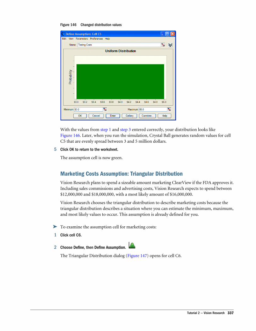
Figure 146 Changed distribution values
With the values from step 1 and step 3 entered correctly, your distribution looks likeFigure 146. Later, when you run the simulation, Crystal Ball generates random values for cellC5 that are evenly spread between 3 and 5 million dollars.
5 Click OK to return to the worksheet.
The assumption cell is now green.
Marketing Costs Assumption: Triangular DistributionVision Research plans to spend a sizeable amount marketing ClearView if the FDA approves it.Including sales commissions and advertising costs, Vision Research expects to spend between$12,000,000 and $18,000,000, with a most likely amount of $16,000,000.
Vision Research chooses the triangular distribution to describe marketing costs because thetriangular distribution describes a situation where you can estimate the minimum, maximum,and most likely values to occur. This assumption is already defined for you.
ä To examine the assumption cell for marketing costs:
1 Click cell C6.
2 Choose Define, then Define Assumption.
The Triangular Distribution dialog (Figure 147) opens for cell C6.
Tutorial 2 — Vision Research 337
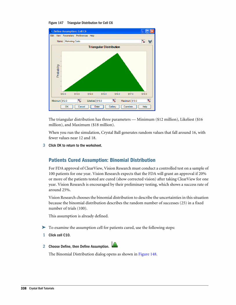
Figure 147 Triangular Distribution for Cell C6
The triangular distribution has three parameters — Minimum ($12 million), Likeliest ($16million), and Maximum ($18 million).
When you run the simulation, Crystal Ball generates random values that fall around 16, withfewer values near 12 and 18.
3 Click OK to return to the worksheet.
Patients Cured Assumption: Binomial DistributionFor FDA approval of ClearView, Vision Research must conduct a controlled test on a sample of100 patients for one year. Vision Research expects that the FDA will grant an approval if 20%or more of the patients tested are cured (show corrected vision) after taking ClearView for oneyear. Vision Research is encouraged by their preliminary testing, which shows a success rate ofaround 25%.
Vision Research chooses the binomial distribution to describe the uncertainties in this situationbecause the binomial distribution describes the random number of successes (25) in a fixednumber of trials (100).
This assumption is already defined.
ä To examine the assumption cell for patients cured, use the following steps:
1 Click cell C10.
2 Choose Define, then Define Assumption.
The Binomial Distribution dialog opens as shown in Figure 148.
338 Crystal Ball Tutorials

Figure 148 Binomial Distribution Dialog
The binomial distribution has two parameters: Probability and Trials. Because Vision Researchexperienced a 25% success rate during preliminary testing, the Probability parameter is set to0.25 to show the likelihood of success.
Note: You can express probabilities either as decimals between 0 and 1, such as 0.03, or as wholenumbers followed by the percent sign, such as 3%.
Because the FDA expects Vision Research to test 100 people, the Trials parameter is set to 100.When you run the simulation, Crystal Ball generates random integers between 0 and 100,simulating the number of patients that would be cured in the FDA test.
3 Click OK to return to the worksheet.
Growth Rate Assumption: Custom DistributionVision Research has determined that nearsightedness afflicts nearly 40 million people in theUnited States, and an additional 0% to 5% of these people will develop this condition duringthe year in which ClearView is tested.
However, the marketing department has learned that a 25% chance exists that a competingproduct will be released on the market soon. This product would decrease ClearView’s potentialmarket by 5% to 15%.
Since the uncertainties in this situation require a unique approach, Vision Research choosesCrystal Ball’s custom distribution to define the growth rate.
The method for specifying parameters in the custom distribution is quite unlike the otherdistribution types, so follow the directions carefully. If you make a mistake, click Gallery to returnto the distribution gallery, then start again at step 4.
Tutorial 2 — Vision Research 339
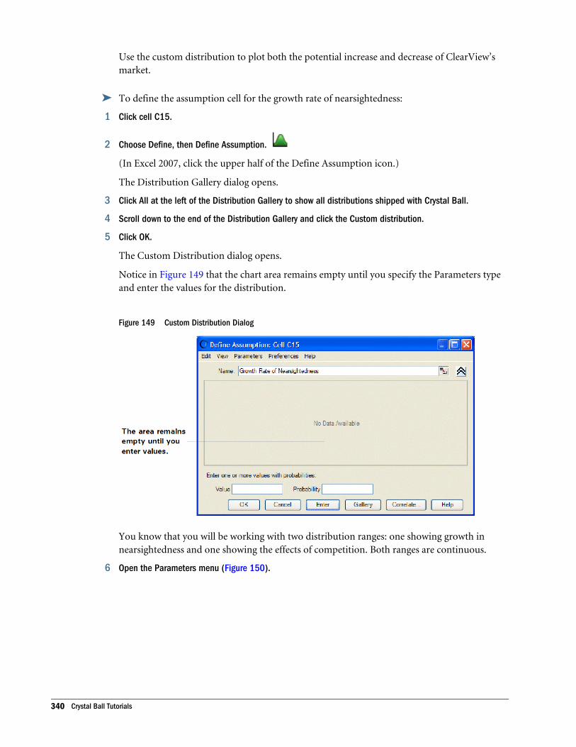
Use the custom distribution to plot both the potential increase and decrease of ClearView’smarket.
ä To define the assumption cell for the growth rate of nearsightedness:
1 Click cell C15.
2 Choose Define, then Define Assumption.
(In Excel 2007, click the upper half of the Define Assumption icon.)
The Distribution Gallery dialog opens.
3 Click All at the left of the Distribution Gallery to show all distributions shipped with Crystal Ball.
4 Scroll down to the end of the Distribution Gallery and click the Custom distribution.
5 Click OK.
The Custom Distribution dialog opens.
Notice in Figure 149 that the chart area remains empty until you specify the Parameters typeand enter the values for the distribution.
Figure 149 Custom Distribution Dialog
You know that you will be working with two distribution ranges: one showing growth innearsightedness and one showing the effects of competition. Both ranges are continuous.
6 Open the Parameters menu (Figure 150).
340 Crystal Ball Tutorials
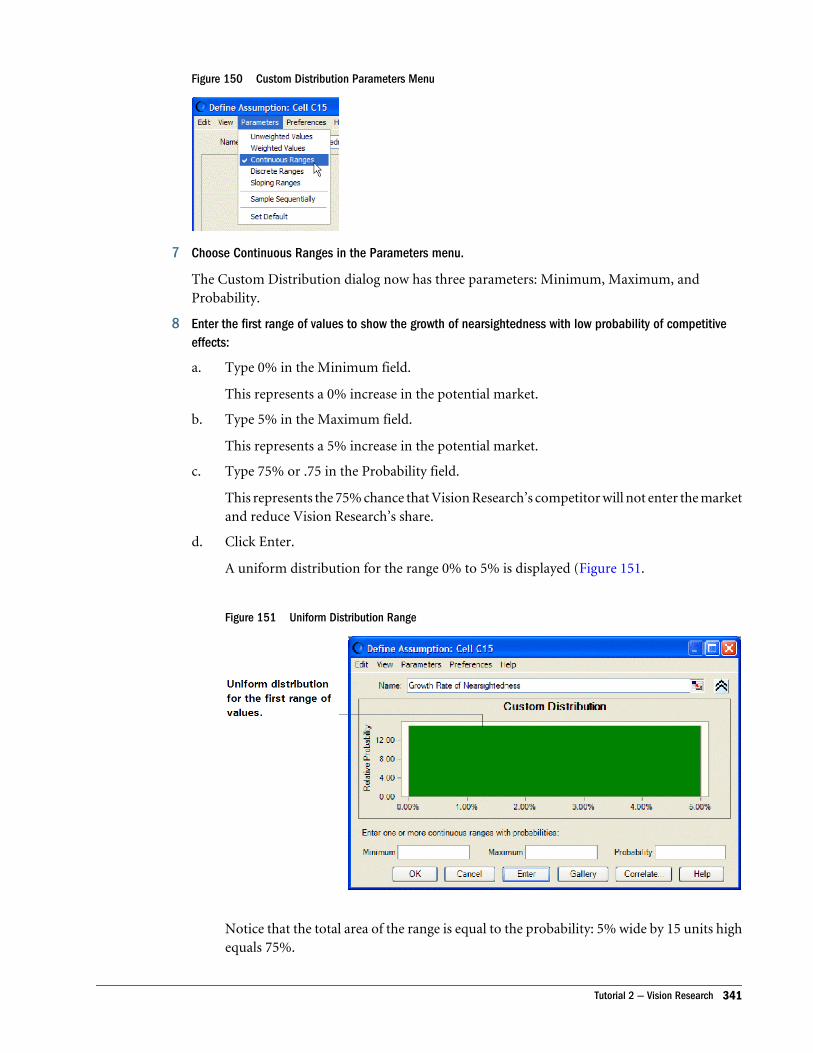
Figure 150 Custom Distribution Parameters Menu
7 Choose Continuous Ranges in the Parameters menu.
The Custom Distribution dialog now has three parameters: Minimum, Maximum, andProbability.
8 Enter the first range of values to show the growth of nearsightedness with low probability of competitiveeffects:
a. Type 0% in the Minimum field.
This represents a 0% increase in the potential market.
b. Type 5% in the Maximum field.
This represents a 5% increase in the potential market.
c. Type 75% or .75 in the Probability field.
This represents the 75% chance that Vision Research’s competitor will not enter the marketand reduce Vision Research’s share.
d. Click Enter.
A uniform distribution for the range 0% to 5% is displayed (Figure 151.
Figure 151 Uniform Distribution Range
Notice that the total area of the range is equal to the probability: 5% wide by 15 units highequals 75%.
Tutorial 2 — Vision Research 341
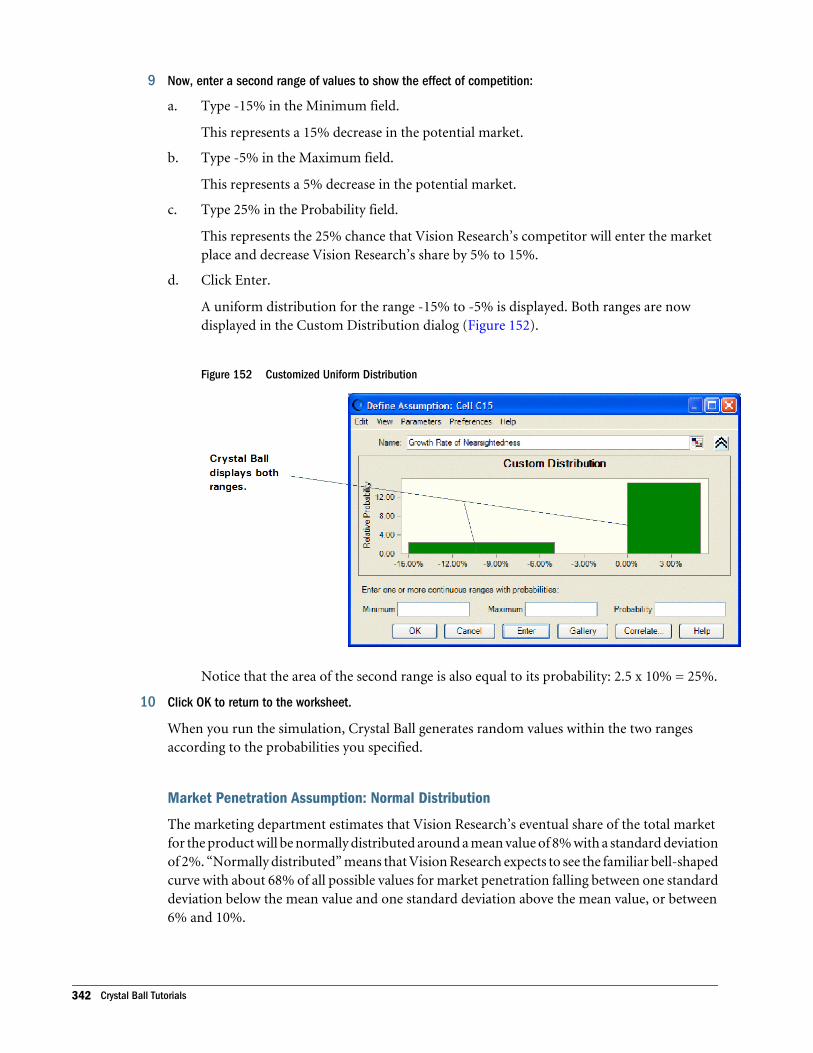
9 Now, enter a second range of values to show the effect of competition:
a. Type -15% in the Minimum field.
This represents a 15% decrease in the potential market.
b. Type -5% in the Maximum field.
This represents a 5% decrease in the potential market.
c. Type 25% in the Probability field.
This represents the 25% chance that Vision Research’s competitor will enter the marketplace and decrease Vision Research’s share by 5% to 15%.
d. Click Enter.
A uniform distribution for the range -15% to -5% is displayed. Both ranges are nowdisplayed in the Custom Distribution dialog (Figure 152).
Figure 152 Customized Uniform Distribution
Notice that the area of the second range is also equal to its probability: 2.5 x 10% = 25%.
10 Click OK to return to the worksheet.
When you run the simulation, Crystal Ball generates random values within the two rangesaccording to the probabilities you specified.
Market Penetration Assumption: Normal Distribution
The marketing department estimates that Vision Research’s eventual share of the total marketfor the product will be normally distributed around a mean value of 8% with a standard deviationof 2%. “Normally distributed” means that Vision Research expects to see the familiar bell-shapedcurve with about 68% of all possible values for market penetration falling between one standarddeviation below the mean value and one standard deviation above the mean value, or between6% and 10%.
342 Crystal Ball Tutorials
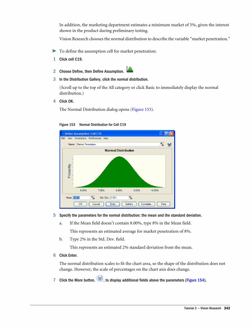
In addition, the marketing department estimates a minimum market of 5%, given the interestshown in the product during preliminary testing.
Vision Research chooses the normal distribution to describe the variable “market penetration.”
ä To define the assumption cell for market penetration:
1 Click cell C19.
2 Choose Define, then Define Assumption.
3 In the Distribution Gallery, click the normal distribution.
(Scroll up to the top of the All category or click Basic to immediately display the normaldistribution.)
4 Click OK.
The Normal Distribution dialog opens (Figure 153).
Figure 153 Normal Distribution for Cell C19
5 Specify the parameters for the normal distribution: the mean and the standard deviation.
a. If the Mean field doesn’t contain 8.00%, type 8% in the Mean field.
This represents an estimated average for market penetration of 8%.
b. Type 2% in the Std. Dev. field.
This represents an estimated 2% standard deviation from the mean.
6 Click Enter.
The normal distribution scales to fit the chart area, so the shape of the distribution does notchange. However, the scale of percentages on the chart axis does change.
7 Click the More button, , to display additional fields above the parameters (Figure 154).
Tutorial 2 — Vision Research 343
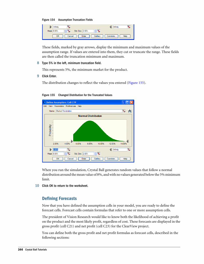
Figure 154 Assumption Truncation Fields
These fields, marked by gray arrows, display the minimum and maximum values of theassumption range. If values are entered into them, they cut or truncate the range. These fieldsare then called the truncation minimum and maximum.
8 Type 5% in the left, minimum truncation field.
This represents 5%, the minimum market for the product.
9 Click Enter.
The distribution changes to reflect the values you entered (Figure 155).
Figure 155 Changed Distribution for the Truncated Values
When you run the simulation, Crystal Ball generates random values that follow a normaldistribution around the mean value of 8%, and with no values generated below the 5% minimumlimit.
10 Click OK to return to the worksheet.
Defining ForecastsNow that you have defined the assumption cells in your model, you are ready to define theforecast cells. Forecast cells contain formulas that refer to one or more assumption cells.
The president of Vision Research would like to know both the likelihood of achieving a profiton the product and the most likely profit, regardless of cost. These forecasts are displayed in thegross profit (cell C21) and net profit (cell C23) for the ClearView project.
You can define both the gross profit and net profit formulas as forecast cells, described in thefollowing sections:
344 Crystal Ball Tutorials
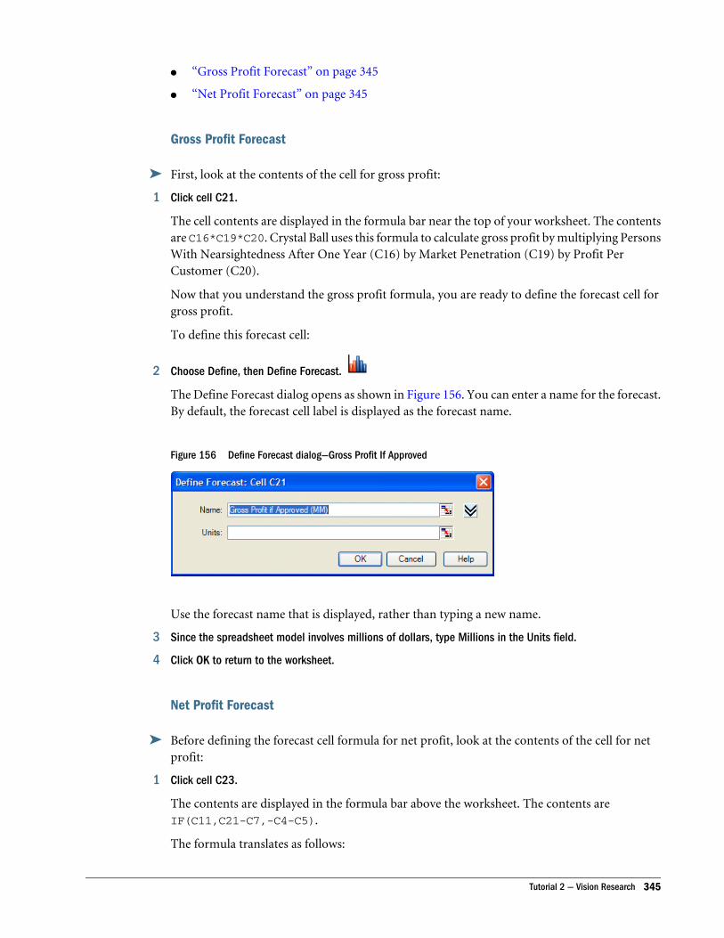
l “Gross Profit Forecast” on page 345
l “Net Profit Forecast” on page 345
Gross Profit Forecast
ä First, look at the contents of the cell for gross profit:
1 Click cell C21.
The cell contents are displayed in the formula bar near the top of your worksheet. The contentsare C16*C19*C20. Crystal Ball uses this formula to calculate gross profit by multiplying PersonsWith Nearsightedness After One Year (C16) by Market Penetration (C19) by Profit PerCustomer (C20).
Now that you understand the gross profit formula, you are ready to define the forecast cell forgross profit.
To define this forecast cell:
2 Choose Define, then Define Forecast.
The Define Forecast dialog opens as shown in Figure 156. You can enter a name for the forecast.By default, the forecast cell label is displayed as the forecast name.
Figure 156 Define Forecast dialog—Gross Profit If Approved
Use the forecast name that is displayed, rather than typing a new name.
3 Since the spreadsheet model involves millions of dollars, type Millions in the Units field.
4 Click OK to return to the worksheet.
Net Profit Forecast
ä Before defining the forecast cell formula for net profit, look at the contents of the cell for netprofit:
1 Click cell C23.
The contents are displayed in the formula bar above the worksheet. The contents areIF(C11,C21-C7,-C4-C5).
The formula translates as follows:
Tutorial 2 — Vision Research 345
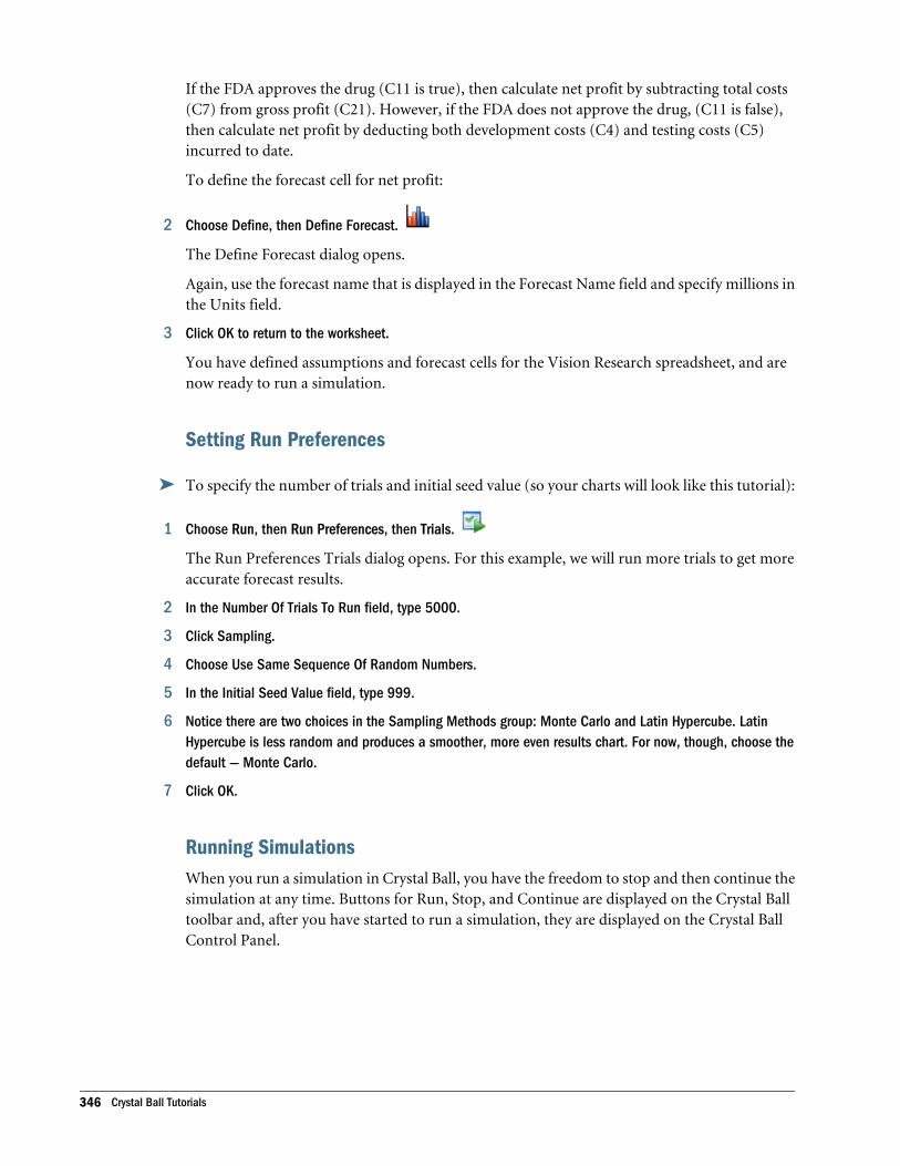
If the FDA approves the drug (C11 is true), then calculate net profit by subtracting total costs(C7) from gross profit (C21). However, if the FDA does not approve the drug, (C11 is false),then calculate net profit by deducting both development costs (C4) and testing costs (C5)incurred to date.
To define the forecast cell for net profit:
2 Choose Define, then Define Forecast.
The Define Forecast dialog opens.
Again, use the forecast name that is displayed in the Forecast Name field and specify millions inthe Units field.
3 Click OK to return to the worksheet.
You have defined assumptions and forecast cells for the Vision Research spreadsheet, and arenow ready to run a simulation.
Setting Run Preferences
ä To specify the number of trials and initial seed value (so your charts will look like this tutorial):
1 Choose Run, then Run Preferences, then Trials.
The Run Preferences Trials dialog opens. For this example, we will run more trials to get moreaccurate forecast results.
2 In the Number Of Trials To Run field, type 5000.
3 Click Sampling.
4 Choose Use Same Sequence Of Random Numbers.
5 In the Initial Seed Value field, type 999.
6 Notice there are two choices in the Sampling Methods group: Monte Carlo and Latin Hypercube. LatinHypercube is less random and produces a smoother, more even results chart. For now, though, choose thedefault — Monte Carlo.
7 Click OK.
Running SimulationsWhen you run a simulation in Crystal Ball, you have the freedom to stop and then continue thesimulation at any time. Buttons for Run, Stop, and Continue are displayed on the Crystal Balltoolbar and, after you have started to run a simulation, they are displayed on the Crystal BallControl Panel.
346 Crystal Ball Tutorials
ä To run the simulation, click Run, .
Interpreting the ResultsNow that you have run the simulation, you are ready to interpret the forecast results. ShouldVision Research scrap the ClearView project or proceed to develop and market this revolutionarynew drug? For the answer, review the forecast charts.
The following sections describe how to analyze results for this scenario:
l “Reviewing the Net Profit Forecast Chart” on page 347
l “Determining the Net Profit Certainty Level” on page 348
l “Customizing Forecast Charts” on page 350
Note: Crystal Ball windows are separate from Excel windows. If Crystal Ball’s windows or chartsdisappear from your screen, they are usually simply behind the main Excel window. Tobring them to the front, click the Crystal Ball icon in the Windows taskbar or press Alt
+Tab and choose Crystal Ball, .
Note: To display forecast charts in Excel 2007, choose Analyze, then View Charts, then ForecastCharts.
Reviewing the Net Profit Forecast Chart
Forecast charts are frequency distributions. They show the number or frequency of valuesoccurring in a given bin or group interval and show how the frequencies are distributed. InFigure 157, the bin that contains the most values has a frequency of about 280.
Crystal Ball forecasts the entire range of results for the Vision Research project. However, theforecast charts don’t display the most extreme values (outliers). Here, the display range includesvalues from approximately –$15 million to $38 million.
Tutorial 2 — Vision Research 347
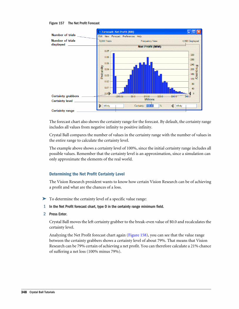
Figure 157 The Net Profit Forecast
The forecast chart also shows the certainty range for the forecast. By default, the certainty rangeincludes all values from negative infinity to positive infinity.
Crystal Ball compares the number of values in the certainty range with the number of values inthe entire range to calculate the certainty level.
The example above shows a certainty level of 100%, since the initial certainty range includes allpossible values. Remember that the certainty level is an approximation, since a simulation canonly approximate the elements of the real world.
Determining the Net Profit Certainty Level
The Vision Research president wants to know how certain Vision Research can be of achievinga profit and what are the chances of a loss.
ä To determine the certainty level of a specific value range:
1 In the Net Profit forecast chart, type 0 in the certainty range minimum field.
2 Press Enter.
Crystal Ball moves the left certainty grabber to the break-even value of $0.0 and recalculates thecertainty level.
Analyzing the Net Profit forecast chart again (Figure 158), you can see that the value rangebetween the certainty grabbers shows a certainty level of about 79%. That means that VisionResearch can be 79% certain of achieving a net profit. You can therefore calculate a 21% chanceof suffering a net loss (100% minus 79%).
348 Crystal Ball Tutorials

Figure 158 Net Profit Forecast—$0 Minimum
Now, the president of Vision Research would like to know the certainty of achieving a minimumprofit of $2,000,000. With Crystal Ball, you can easily answer this question.
ä To do so:
1 Type 2 in the certainty range minimum field.
2 Press Enter.
As Figure 159 shows, Crystal Ball moves the left certainty grabber to $2.0 and recalculates thecertainty level. Vision Research can be about 72% certain of achieving a minimum net profit of$2,000,000.
Figure 159 Recalculated Certainty Level
Vision Research is encouraged by the forecast result. The president now wants to know howcertain Vision Research can be of achieving a minimum net profit of $4,000,000. If Crystal Ball
Tutorial 2 — Vision Research 349
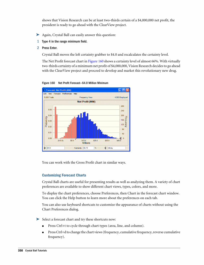
shows that Vision Research can be at least two-thirds certain of a $4,000,000 net profit, thepresident is ready to go ahead with the ClearView project.
ä Again, Crystal Ball can easily answer this question:
1 Type 4 in the range minimum field.
2 Press Enter.
Crystal Ball moves the left certainty grabber to $4.0 and recalculates the certainty level.
The Net Profit forecast chart in Figure 160 shows a certainty level of almost 66%. With virtuallytwo-thirds certainty of a minimum net profit of $4,000,000, Vision Research decides to go aheadwith the ClearView project and proceed to develop and market this revolutionary new drug.
Figure 160 Net Profit Forecast—$4.0 Million Minimum
You can work with the Gross Profit chart in similar ways.
Customizing Forecast Charts
Crystal Ball charts are useful for presenting results as well as analyzing them. A variety of chartpreferences are available to show different chart views, types, colors, and more.
To display the chart preferences, choose Preferences, then Chart in the forecast chart window.You can click the Help button to learn more about the preferences on each tab.
You can also use keyboard shortcuts to customize the appearance of charts without using theChart Preferences dialog.
ä Select a forecast chart and try these shortcuts now:
l Press Ctrl+t to cycle through chart types (area, line, and column).
l Press Ctrl+d to change the chart views (frequency, cumulative frequency, reverse cumulativefrequency).
350 Crystal Ball Tutorials
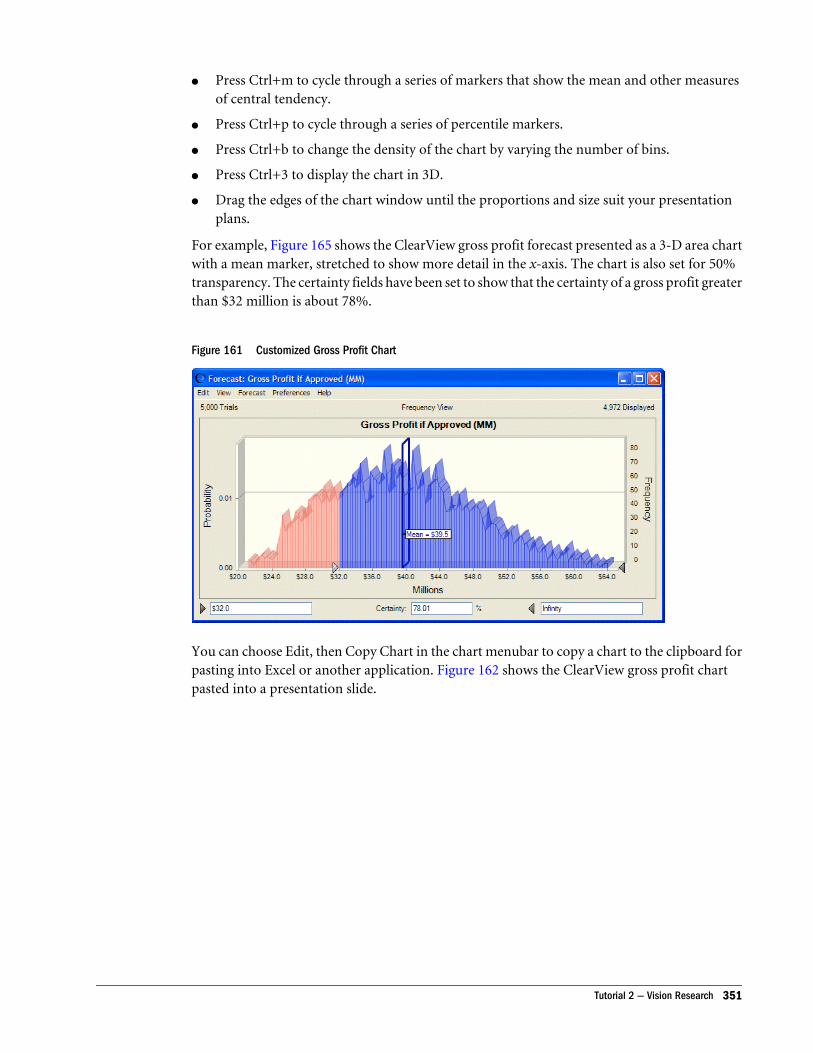
l Press Ctrl+m to cycle through a series of markers that show the mean and other measuresof central tendency.
l Press Ctrl+p to cycle through a series of percentile markers.
l Press Ctrl+b to change the density of the chart by varying the number of bins.
l Press Ctrl+3 to display the chart in 3D.
l Drag the edges of the chart window until the proportions and size suit your presentationplans.
For example, Figure 165 shows the ClearView gross profit forecast presented as a 3-D area chartwith a mean marker, stretched to show more detail in the x-axis. The chart is also set for 50%transparency. The certainty fields have been set to show that the certainty of a gross profit greaterthan $32 million is about 78%.
Figure 161 Customized Gross Profit Chart
You can choose Edit, then Copy Chart in the chart menubar to copy a chart to the clipboard forpasting into Excel or another application. Figure 162 shows the ClearView gross profit chartpasted into a presentation slide.
Tutorial 2 — Vision Research 351
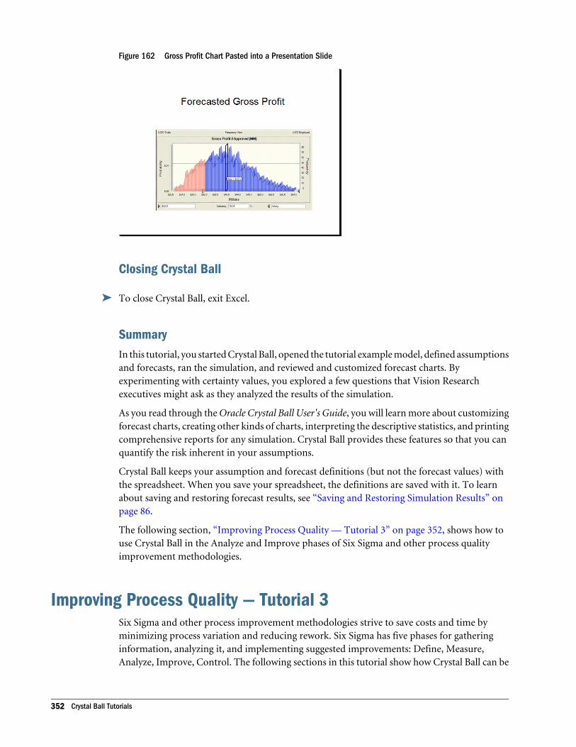
Figure 162 Gross Profit Chart Pasted into a Presentation Slide
Closing Crystal Ball
ä To close Crystal Ball, exit Excel.
SummaryIn this tutorial, you started Crystal Ball, opened the tutorial example model, defined assumptionsand forecasts, ran the simulation, and reviewed and customized forecast charts. Byexperimenting with certainty values, you explored a few questions that Vision Researchexecutives might ask as they analyzed the results of the simulation.
As you read through the Oracle Crystal Ball User's Guide, you will learn more about customizingforecast charts, creating other kinds of charts, interpreting the descriptive statistics, and printingcomprehensive reports for any simulation. Crystal Ball provides these features so that you canquantify the risk inherent in your assumptions.
Crystal Ball keeps your assumption and forecast definitions (but not the forecast values) withthe spreadsheet. When you save your spreadsheet, the definitions are saved with it. To learnabout saving and restoring forecast results, see “Saving and Restoring Simulation Results” onpage 86.
The following section, “Improving Process Quality — Tutorial 3” on page 352, shows how touse Crystal Ball in the Analyze and Improve phases of Six Sigma and other process qualityimprovement methodologies.
Improving Process Quality — Tutorial 3Six Sigma and other process improvement methodologies strive to save costs and time byminimizing process variation and reducing rework. Six Sigma has five phases for gatheringinformation, analyzing it, and implementing suggested improvements: Define, Measure,Analyze, Improve, Control. The following sections in this tutorial show how Crystal Ball can be
352 Crystal Ball Tutorials

used in the Analyze and Improve phases to discover inconsistencies and reduce variation in abank’s loan processing system:
l “Overall Approach” on page 353
l “Using the Loan Processing Model” on page 355
“Packaging Pump Design — Tutorial 4” on page 366, shows how to use Crystal Ball in designquality programs such as Design for Six Sigma (DFSS).
Overall ApproachSuppose you are assigned the task of improving loan processing quality at a bank. You want tominimize average processing time, keeping below the bank’s target. At the same time, you wantto evaluate and improve processing time consistency using the following techniques:
l Define — You plan to talk with stakeholders in various departments to learn how they arecurrently working, how they view of the problem, and what outcome they hope to see.
l Measure — You will determine current processing times and the amount of variation withinthem.
l Analyze — You plan to use Crystal Ball to help you discover process capability, or howclosely the processing times map to process requirements.
l Improve — You will use information gathered in the previous phases to design andimplement improvements in processing time and consistency.
l Control — You need to ensure permanent improvements by setting up a system of feedbackloops to continuously measure process results and change the output if measures exceeddesired control targets and control limits.
In the Define and Measure phases, you obtain and use information to build a Crystal Ball model.Then, you use Crystal Ball to simulate real-world variations that occur in processing loans.Finally, you can use sensitivity analysis and further optimization to arrive at the best balancebetween time and consistency.
The following sections give details of each phase:
l “Define Phase” on page 353
l “Measure Phase” on page 354
l “Analyze Phase” on page 354
l “Improve Phase” on page 354
l “Control Phase” on page 355
Define PhaseThe bank’s loan processing procedures involve six steps. You interview staff involved with eachstep and learn that marketing and management groups are hoping for completion of all six stepswithin 96 working hours. Based on these interviews, you establish both the target and upper
Improving Process Quality — Tutorial 3 353
specification limit (USL) at 96 hours. There is no lower specification limit (LSL), althoughconsistency (the sigma level) seems to be an issue. You decide to obtain more concrete data.
Measure PhaseYou document time and time variation data for each processing step, as follows:
l Customer Inquiry involves the creation of an initial rate quote following the first customercontact by phone, in-person visit, or the Internet. Historical data indicates this cycle time islognormally distributed with a mean of one hour and a standard deviation of 0.25 hours.
l Loan Application involves the completion of forms by customers, with or without staffassistance. This step takes from one to five eight-hour days, but usually takes three days.
l Document Verification and processing occurs in the bank, where a loan specialist reviewscredit data, presents loan alternatives to customers, and independently verifies information.This step usually takes between two and four eight-hour days. However, about two out often times, the loan is suspended and takes between four and six days for additional reviewsand documentation.
l Underwriting, or loan approval, usually takes from one hour to 8 hours. All lengths of timehave the same likelihood of occurrence.
l Loan Closing includes the preparation of the final documentation, locking in an interestrate, and arranging where to deposit funds. Historical data show that this step has a meanof two days, but you don’t yet know how the data are distributed.
l Loan Disbursement, moving the funds to the customer’s bank, usually takes 16 hours, withsome variation. Two-thirds of disbursement times fall within 12 and 20 hours.
After gathering this information, you decide to load it into Excel and use Crystal Ball to analyzeit.
Analyze PhaseDuring the Analyze phase, you create an Excel workbook that includes historical data on loanclosing times. Then, you can capture the time and variation information for each step as a CrystalBall assumption. Finally, you can define overall processing time as a Crystal Ball forecast. Whenthe simulation runs, you can view capability metrics to gain insight into the degree of processvariation, or inconsistency. You can also generate a sensitivity chart to learn more about themain sources of inconsistency.
“Using the Loan Processing Model” on page 355, shows how to use a Crystal Ball model in theAnalyze and Improve phases to accomplish your quality goals.
Improve PhaseYou can experiment with the effects of changing the main sources of inconsistency. If you haveOptQuest, you can also define decision variables and optimize for the shortest processing timeand least time variation.
354 Crystal Ball Tutorials
Control PhaseYou set up a system of measuring cycle times for each step and analyzing them on a regular basis.You run a Crystal Ball simulation on real data once a month with a program of corrective actionsto take whenever results exceed desired limits by a specified amount.
Using the Loan Processing ModelThis section shows how to construct a model that effectively simulates each step of the loanprocess with dual goals of minimizing processing time and maximizing time consistency. Then,you run the model and analyze the output using Crystal Ball’s process capability features.
The following sections describe how to work with the loan processing model and analyze datafrom it:
l “Introduction” on page 325
l “Activating the Process Capability Features” on page 355
l “Setting the Sampling Seed Value” on page 356
l “Opening the Example Model” on page 333
l “Reviewing the Vision Research Scenario” on page 334
l “Reviewing the Assumptions” on page 357
l “Reviewing the Forecast” on page 359
l “Running Simulations” on page 360
l “Analyzing Simulations” on page 360
l “Investigating Improvement Possibilities” on page 362
Starting Crystal BallIf Crystal Ball is not already started, start it as usual (“Starting Crystal Ball” on page 326). If theCrystal Ball Welcome screen opens, check Quality in the upper left, and then click Use CrystalBall at the right.
Activating the Process Capability Features
ä To confirm that the process capability features have been activated and activate them, ifnecessary:
1 Choose Run, then Run Preferences.
2 Click the Statistics tab in the Run Preferences dialog.
3 Check Calculate Capability Metrics.
4 Click the Options button to confirm the settings.
Improving Process Quality — Tutorial 3 355
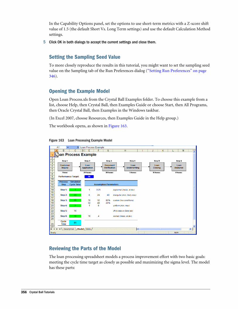
In the Capability Options panel, set the options to use short-term metrics with a Z-score shiftvalue of 1.5 (the default Short Vs. Long Term settings) and use the default Calculation Methodsettings.
5 Click OK in both dialogs to accept the current settings and close them.
Setting the Sampling Seed ValueTo more closely reproduce the results in this tutorial, you might want to set the sampling seedvalue on the Sampling tab of the Run Preferences dialog (“Setting Run Preferences” on page346).
Opening the Example ModelOpen Loan Process.xls from the Crystal Ball Examples folder. To choose this example from alist, choose Help, then Crystal Ball, then Examples Guide or choose Start, then All Programs,then Oracle Crystal Ball, then Examples in the Windows taskbar.
(In Excel 2007, choose Resources, then Examples Guide in the Help group.)
The workbook opens, as shown in Figure 163.
Figure 163 Loan Processing Example Model
Reviewing the Parts of the ModelThe loan processing spreadsheet models a process improvement effort with two basic goals:meeting the cycle time target as closely as possible and maximizing the sigma level. The modelhas these parts:
356 Crystal Ball Tutorials
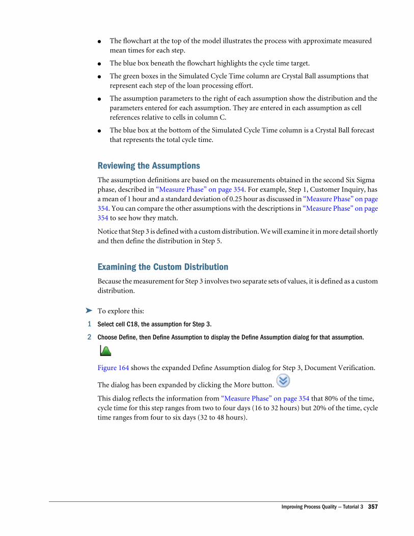
l The flowchart at the top of the model illustrates the process with approximate measuredmean times for each step.
l The blue box beneath the flowchart highlights the cycle time target.
l The green boxes in the Simulated Cycle Time column are Crystal Ball assumptions thatrepresent each step of the loan processing effort.
l The assumption parameters to the right of each assumption show the distribution and theparameters entered for each assumption. They are entered in each assumption as cellreferences relative to cells in column C.
l The blue box at the bottom of the Simulated Cycle Time column is a Crystal Ball forecastthat represents the total cycle time.
Reviewing the AssumptionsThe assumption definitions are based on the measurements obtained in the second Six Sigmaphase, described in “Measure Phase” on page 354. For example, Step 1, Customer Inquiry, hasa mean of 1 hour and a standard deviation of 0.25 hour as discussed in “Measure Phase” on page354. You can compare the other assumptions with the descriptions in “Measure Phase” on page354 to see how they match.
Notice that Step 3 is defined with a custom distribution. We will examine it in more detail shortlyand then define the distribution in Step 5.
Examining the Custom DistributionBecause the measurement for Step 3 involves two separate sets of values, it is defined as a customdistribution.
ä To explore this:
1 Select cell C18, the assumption for Step 3.
2 Choose Define, then Define Assumption to display the Define Assumption dialog for that assumption.
Figure 164 shows the expanded Define Assumption dialog for Step 3, Document Verification.
The dialog has been expanded by clicking the More button.
This dialog reflects the information from “Measure Phase” on page 354 that 80% of the time,cycle time for this step ranges from two to four days (16 to 32 hours) but 20% of the time, cycletime ranges from four to six days (32 to 48 hours).
Improving Process Quality — Tutorial 3 357
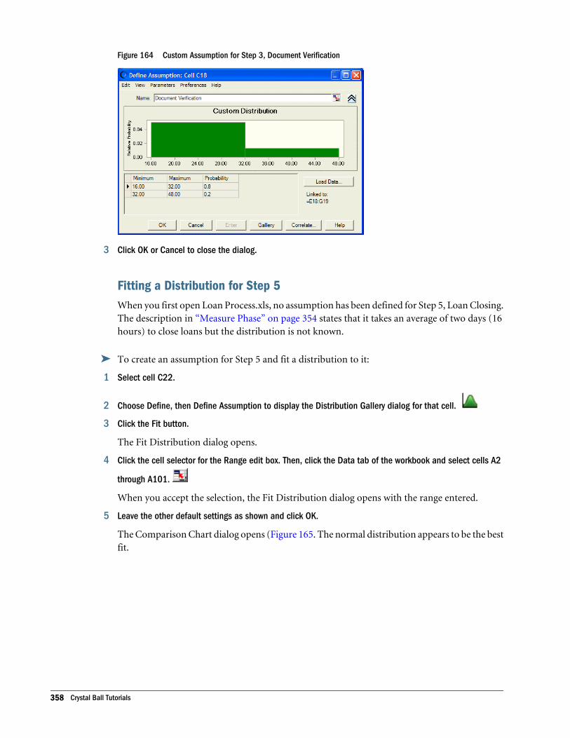
Figure 164 Custom Assumption for Step 3, Document Verification
3 Click OK or Cancel to close the dialog.
Fitting a Distribution for Step 5When you first open Loan Process.xls, no assumption has been defined for Step 5, Loan Closing.The description in “Measure Phase” on page 354 states that it takes an average of two days (16hours) to close loans but the distribution is not known.
ä To create an assumption for Step 5 and fit a distribution to it:
1 Select cell C22.
2 Choose Define, then Define Assumption to display the Distribution Gallery dialog for that cell.
3 Click the Fit button.
The Fit Distribution dialog opens.
4 Click the cell selector for the Range edit box. Then, click the Data tab of the workbook and select cells A2
through A101.
When you accept the selection, the Fit Distribution dialog opens with the range entered.
5 Leave the other default settings as shown and click OK.
The Comparison Chart dialog opens (Figure 165. The normal distribution appears to be the bestfit.
358 Crystal Ball Tutorials
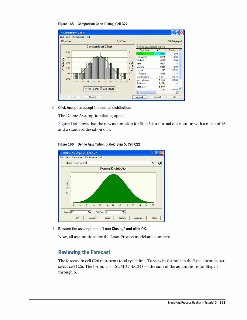
Figure 165 Comparison Chart Dialog, Cell C22
6 Click Accept to accept the normal distribution.
The Define Assumption dialog opens.
Figure 166 shows that the new assumption for Step 5 is a normal distribution with a mean of 16and a standard deviation of 4.
Figure 166 Define Assumption Dialog, Step 5, Cell C22
7 Rename the assumption to "Loan Closing" and click OK.
Now, all assumptions for the Loan Process model are complete.
Reviewing the ForecastThe forecast in cell C26 represents total cycle time. To view its formula in the Excel formula bar,select cell C26. The formula is =SUM(C14:C24) — the sum of the assumptions for Steps 1through 6.
Improving Process Quality — Tutorial 3 359
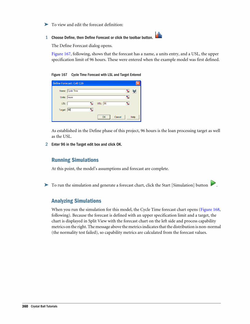
ä To view and edit the forecast definition:
1 Choose Define, then Define Forecast or click the toolbar button.
The Define Forecast dialog opens.
Figure 167, following, shows that the forecast has a name, a units entry, and a USL, the upperspecification limit of 96 hours. These were entered when the example model was first defined.
Figure 167 Cycle Time Forecast with LSL and Target Entered
As established in the Define phase of this project, 96 hours is the loan processing target as wellas the USL.
2 Enter 96 in the Target edit box and click OK.
Running SimulationsAt this point, the model’s assumptions and forecast are complete.
ä To run the simulation and generate a forecast chart, click the Start [Simulation] button .
Analyzing SimulationsWhen you run the simulation for this model, the Cycle Time forecast chart opens (Figure 168,following). Because the forecast is defined with an upper specification limit and a target, thechart is displayed in Split View with the forecast chart on the left side and process capabilitymetrics on the right. The message above the metrics indicates that the distribution is non-normal(the normality test failed), so capability metrics are calculated from the forecast values.
360 Crystal Ball Tutorials
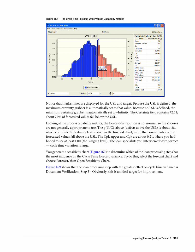
Figure 168 The Cycle Time Forecast with Process Capability Metrics
Notice that marker lines are displayed for the USL and target. Because the USL is defined, themaximum certainty grabber is automatically set to that value. Because no LSL is defined, theminimum certainty grabber is automatically set to –Infinity. The Certainty field contains 72.31;about 72% of forecasted values fall below the USL.
Looking at the process capability metrics, the forecast distribution is not normal, so the Z scoresare not generally appropriate to use. The p(N/C)-above (defects above the USL) is about .28,which confirms the certainty level shown in the forecast chart; more than one-quarter of theforecasted values fall above the USL. The Cpk-upper and Cpk are about 0.21, where you hadhoped to see at least 1.00 (the 3-sigma level). The loan specialists you interviewed were correct— cycle time variation is large.
You generate a sensitivity chart (Figure 169) to determine which of the loan processing steps hasthe most influence on the Cycle Time forecast variance. To do this, select the forecast chart andchoose Forecast, then Open Sensitivity Chart.
Figure 169 shows that the loan processing step with the greatest effect on cycle time variance isDocument Verification (Step 3). Obviously, this is an ideal target for improvement.
Improving Process Quality — Tutorial 3 361
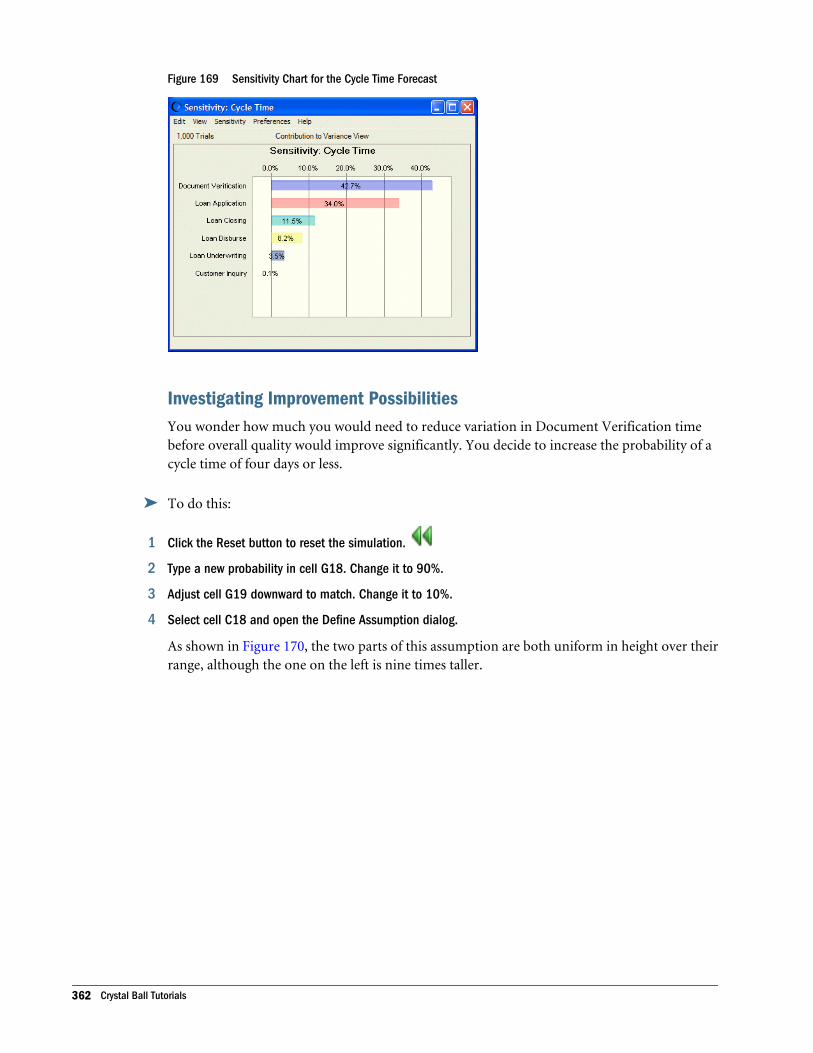
Figure 169 Sensitivity Chart for the Cycle Time Forecast
Investigating Improvement PossibilitiesYou wonder how much you would need to reduce variation in Document Verification timebefore overall quality would improve significantly. You decide to increase the probability of acycle time of four days or less.
ä To do this:
1 Click the Reset button to reset the simulation.
2 Type a new probability in cell G18. Change it to 90%.
3 Adjust cell G19 downward to match. Change it to 10%.
4 Select cell C18 and open the Define Assumption dialog.
As shown in Figure 170, the two parts of this assumption are both uniform in height over theirrange, although the one on the left is nine times taller.
362 Crystal Ball Tutorials

Figure 170 Document Verification Assumption, Adjusted
This assumption was previously displayed in Figure 164. Because the probabilities in the tableare linked to workbook cells, when you adjusted the workbook, you also adjusted the asumptionprobabilities.
5 Close the Define assumption dialog and run the simulation.
6 Review the forecast chart in Figure 171.
Figure 171 The Cycle Time Forecast with Process Capability Metrics
Crystal Ball sets the upper certainty level at the USL/Target value (96). If the lower certaintygrabber is not located at –Infinity, click the lower grabber and drag it to the left end of the chartas shown in Figure 171. Now, the certainty of cycle time falling at or below the USL is about78%. You decide to make a drastic change and edit the assumption parameters for DocumentVerification as follows (change 32 to 24 in the first row; change 90% to 100% and 10% to 0%):
Improving Process Quality — Tutorial 3 363
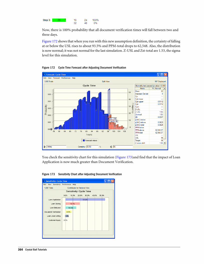
Now, there is 100% probability that all document verification times will fall between two andthree days.
Figure 172 shows that when you run with this new assumption definition, the certainty of fallingat or below the USL rises to about 93.5% and PPM-total drops to 62,548. Also, the distributionis now normal; it was not normal for the last simulation. Z-USL and Zst-total are 1.53, the sigmalevel for this simulation.
Figure 172 Cycle Time Forecast after Adjusting Document Verification
You check the sensitivity chart for this simulation (Figure 173)and find that the impact of LoanApplication is now much greater than Document Verification.
Figure 173 Sensitivity Chart after Adjusting Document Verification
364 Crystal Ball Tutorials
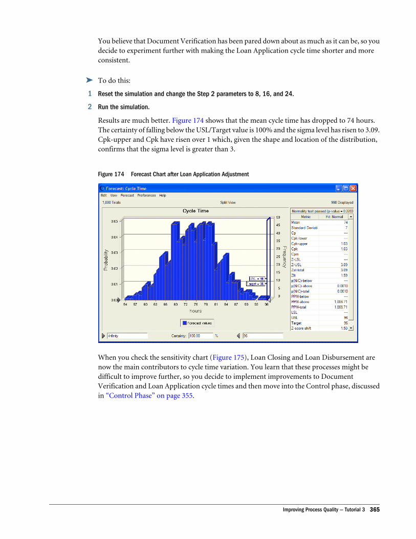
You believe that Document Verification has been pared down about as much as it can be, so youdecide to experiment further with making the Loan Application cycle time shorter and moreconsistent.
ä To do this:
1 Reset the simulation and change the Step 2 parameters to 8, 16, and 24.
2 Run the simulation.
Results are much better. Figure 174 shows that the mean cycle time has dropped to 74 hours.The certainty of falling below the USL/Target value is 100% and the sigma level has risen to 3.09.Cpk-upper and Cpk have risen over 1 which, given the shape and location of the distribution,confirms that the sigma level is greater than 3.
Figure 174 Forecast Chart after Loan Application Adjustment
When you check the sensitivity chart (Figure 175), Loan Closing and Loan Disbursement arenow the main contributors to cycle time variation. You learn that these processes might bedifficult to improve further, so you decide to implement improvements to DocumentVerification and Loan Application cycle times and then move into the Control phase, discussedin “Control Phase” on page 355.
Improving Process Quality — Tutorial 3 365
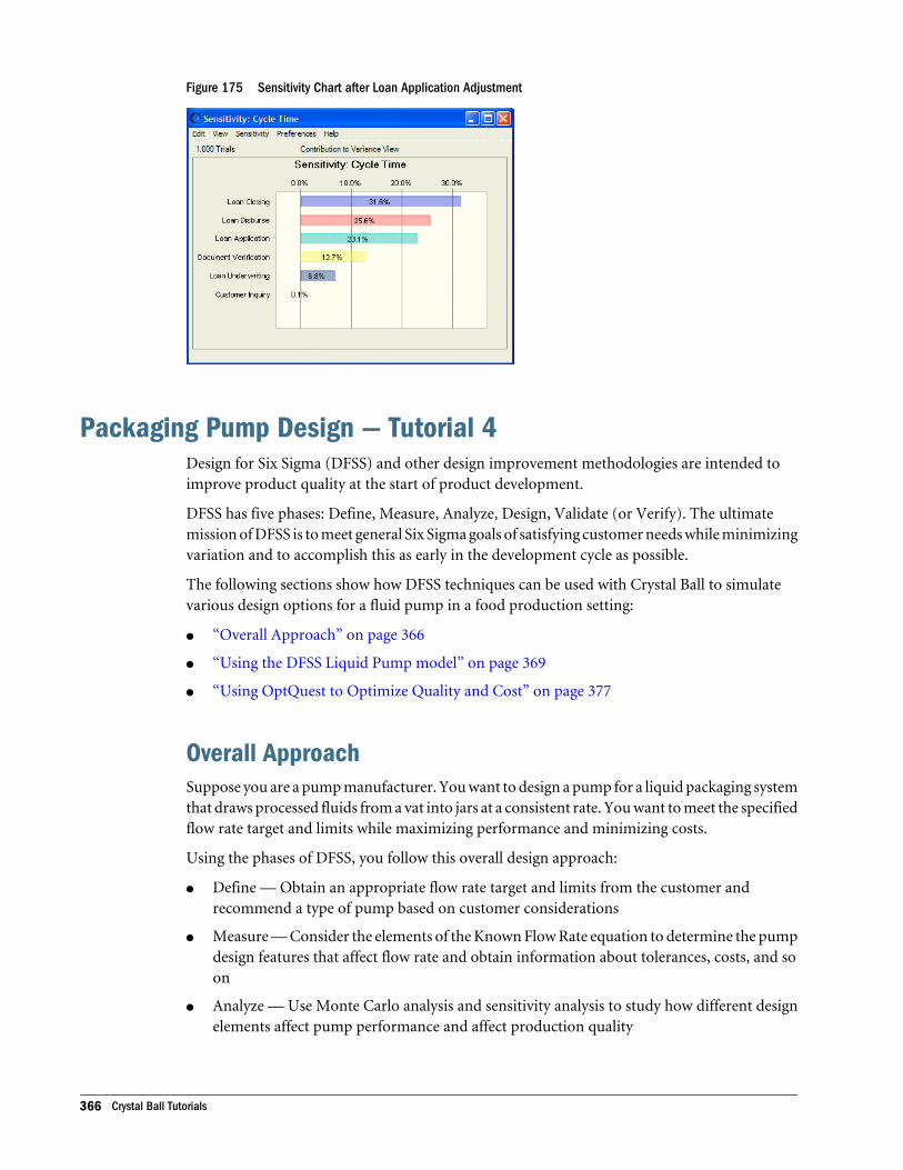
Figure 175 Sensitivity Chart after Loan Application Adjustment
Packaging Pump Design — Tutorial 4Design for Six Sigma (DFSS) and other design improvement methodologies are intended toimprove product quality at the start of product development.
DFSS has five phases: Define, Measure, Analyze, Design, Validate (or Verify). The ultimatemission of DFSS is to meet general Six Sigma goals of satisfying customer needs while minimizingvariation and to accomplish this as early in the development cycle as possible.
The following sections show how DFSS techniques can be used with Crystal Ball to simulatevarious design options for a fluid pump in a food production setting:
l “Overall Approach” on page 366
l “Using the DFSS Liquid Pump model” on page 369
l “Using OptQuest to Optimize Quality and Cost” on page 377
Overall ApproachSuppose you are a pump manufacturer. You want to design a pump for a liquid packaging systemthat draws processed fluids from a vat into jars at a consistent rate. You want to meet the specifiedflow rate target and limits while maximizing performance and minimizing costs.
Using the phases of DFSS, you follow this overall design approach:
l Define — Obtain an appropriate flow rate target and limits from the customer andrecommend a type of pump based on customer considerations
l Measure — Consider the elements of the Known Flow Rate equation to determine the pumpdesign features that affect flow rate and obtain information about tolerances, costs, and soon
l Analyze — Use Monte Carlo analysis and sensitivity analysis to study how different designelements affect pump performance and affect production quality
366 Crystal Ball Tutorials
l Design — Use optimization techniques with defined tradeoffs between flow rateperformance and total cost to determine the design parameters that best meet a definedquality level while reducing cost
l Validate — Based on the optimized design parameters, create physical prototypes and testto confirm that this design configuration yields the best-performing, most cost-effectivepump
In the Define and Measure phases, you obtain and use information to build a Crystal Ball model.Then, you use Crystal Ball to simulate real-world variations that occur in the actualmanufacturing of the product. Finally, if you have Crystal Ball Decision Optimizer, you can usesensitivity analysis and further optimization to arrive at the best balance between quality andcost.
The following sections give details of each phase:
l “Define Phase” on page 367
l “Measure Phase” on page 368
l “Analyze Phase” on page 368
l “Design Phase” on page 368
l “Validate Phase” on page 369
The next main section, “Using the DFSS Liquid Pump model” on page 369, works through thesephases using a Crystal Ball example model.
Define PhaseMarketing and production considerations determine the acceptable range of flow rates basedon how many units should be produced daily to meet market demand, what is useful productiontime per day based on plant setup and productivity, and how many pumps are placed in eachplant.
The food processing company translates marketing requirements into these engineeringspecifications and provides them to you:
l Lower specification limit (LSL) = 47.26 ml/sec
l Upper specification limit (USL) = 53.92 ml/sec
l Target = 50.595 ml/sec
Based on these requirements, you propose a displacement pump with a reciprocating piston.Figure 176, following, shows a basic schematic of the system.
Packaging Pump Design — Tutorial 4 367
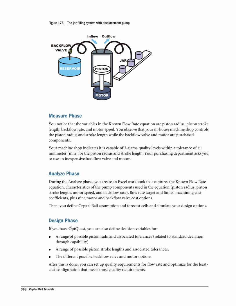
Figure 176 The jar-filling system with displacement pump
Measure PhaseYou notice that the variables in the Known Flow Rate equation are piston radius, piston strokelength, backflow rate, and motor speed. You observe that your in-house machine shop controlsthe piston radius and stroke length while the backflow valve and motor are purchasedcomponents.
Your machine shop indicates it is capable of 3-sigma quality levels within a tolerance of ±1millimeter (mm) for the piston radius and stroke length. Your purchasing department asks youto use an inexpensive backflow valve and motor.
Analyze PhaseDuring the Analyze phase, you create an Excel workbook that captures the Known Flow Rateequation, characteristics of the pump components used in the equation (piston radius, pistonstroke length, motor speed, and backflow rate), flow rate target and limits, machining costcoefficients, plus nine motor and backflow valve cost options.
Then, you define Crystal Ball assumption and forecast cells and simulate your design options.
Design PhaseIf you have OptQuest, you can also define decision variables for:
l A range of possible piston radii and associated tolerances (related to standard deviationthrough capability)
l A range of possible piston stroke lengths and associated tolerances,
l The different possible backflow valve and motor options
After this is done, you can set up quality requirements for flow rate and optimize for the least-cost configuration that meets those quality requirements.
368 Crystal Ball Tutorials
Validate PhaseThis phase involves the physical creation of a prototype based on simulation forecasts followedby physical testing to validate the design. Because so much preliminary work was done withspreadsheet modeling instead of building additional prototypes, a final design can be developedquickly and at minimal cost.
Using the DFSS Liquid Pump modelNow, see how to construct a model that effectively simulates the design process with dual goalsof maximizing quality and minimizing cost. Then, you run the model and analyze the outputusing Crystal Ball’s process capability features.
This tutorial contains the following review and lesson sections::
l “Starting Crystal Ball” on page 369
l “Activating the Process Capability Features” on page 369
l “Setting the Sampling Seed Value” on page 370
l “Opening the Example Model” on page 370
l “Reviewing the Parts of the Model” on page 371
l “Running Simulations” on page 373
l “Analyzing Simulations” on page 373
l “Adjusting Models” on page 375
If you have Crystal Ball Decision Optimizer, see “Using OptQuest to Optimize Quality and Cost”on page 377 for a useful optimization example.
Starting Crystal BallIf Crystal Ball is not already started, start it as usual (“Starting Crystal Ball” on page 326).
Activating the Process Capability Features
ä To confirm that the process capability features have been activated.
1 Choose Run, then Run Preferences.
2 Click the Statistics tab in the Run Preferences dialog.
3 Check Calculate Capability Metrics.
4 Click the Options button to confirm the settings.
For this example, use the defaults: use short-term metrics, calculate metrics from the normaldistribution with a significance level of 0.05, and, if the normality test fails, calculate metricsfrom the forecast values.
5 Click OK in both dialogs to accept the current settings and close them.
Packaging Pump Design — Tutorial 4 369
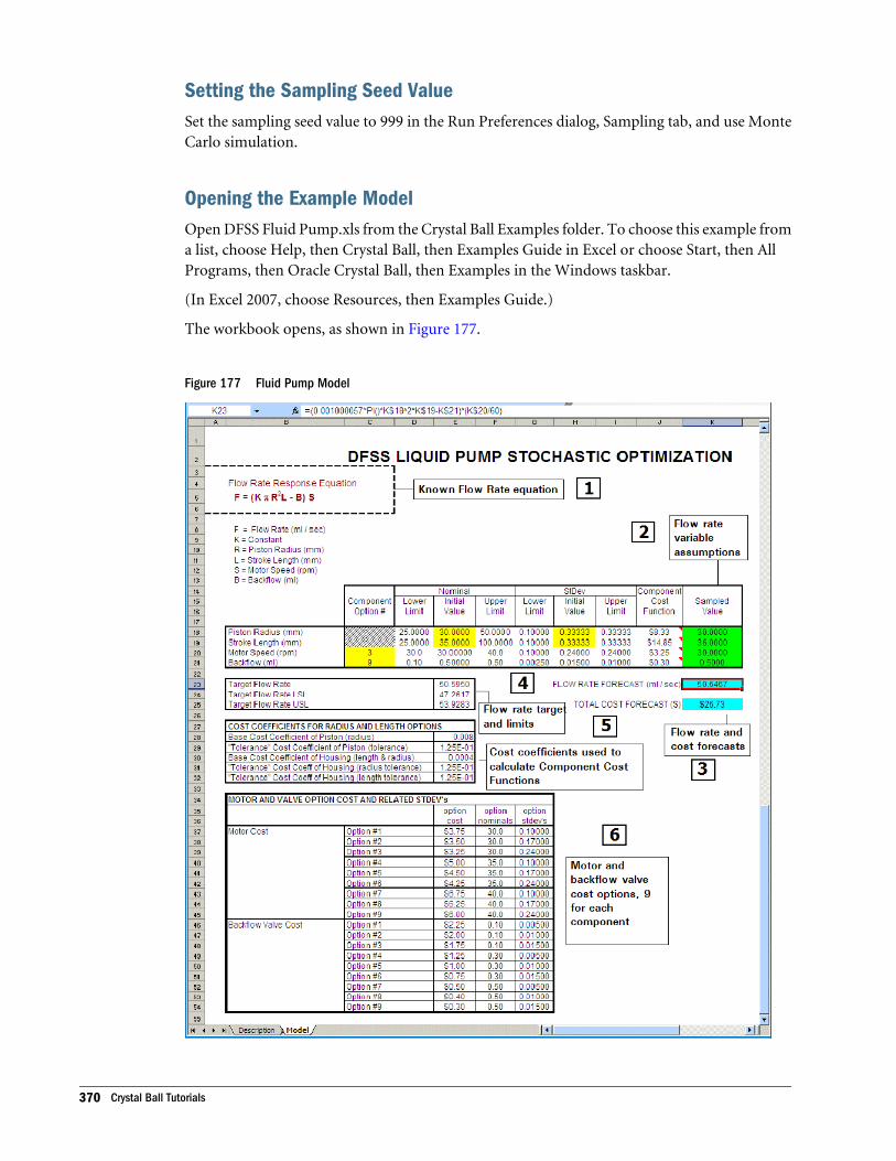
Setting the Sampling Seed ValueSet the sampling seed value to 999 in the Run Preferences dialog, Sampling tab, and use MonteCarlo simulation.
Opening the Example ModelOpen DFSS Fluid Pump.xls from the Crystal Ball Examples folder. To choose this example froma list, choose Help, then Crystal Ball, then Examples Guide in Excel or choose Start, then AllPrograms, then Oracle Crystal Ball, then Examples in the Windows taskbar.
(In Excel 2007, choose Resources, then Examples Guide.)
The workbook opens, as shown in Figure 177.
Figure 177 Fluid Pump Model
370 Crystal Ball Tutorials
This spreadsheet models the fluid pump design problem to be solved.
Reviewing the Parts of the ModelThe liquid pump spreadsheet models a design effort with two basic goals: meeting the flow ratetarget as closely and consistently as possible and minimizing cost. The following sections describesix main parts of the model, indicated by numbers in Figure 177:
l “Known Flow Rate Formula” on page 371
l “Flow Rate Variable Assumptions” on page 371
l “Flow Rate and Cost Forecasts” on page 372
l “Flow Rate Target and Limits” on page 372
l “Cost Coefficients” on page 372
l “Motor and Backflow Valve Cost Options” on page 373
Known Flow Rate Formula
The Known Flow Rate formula specifies the relevant variables discussed earlier: piston radius,piston stroke length, backflow rate, and motor speed.
Flow Rate Variable Assumptions
The flow rate variable assumptions are Crystal Ball assumptions that allow each of the flow ratevariables, listed under the Known Flow Rate formula (1), to be included in the Monte Carlosimulation.
ä To see how these are defined:
1 Select cell K18 and click the Define Assumption button.
2 Optional: Look at K19, K20, and K21.
Each assumption is defined as a normal distribution with a mean equal to the Nominal InitialValue in the column toward the left of the table and a standard deviation equal to the StDevInitial Value in the middle of the table. the Mean and Standard Deviation parameters are notentered directly. Instead, they are entered as cell references to the Initial Value cells in the tableto their left.
Note: In this model, whenever you see the word "nominal," it means approximate, designed, ortheoretical, as opposed to the actual measured value.
Packaging Pump Design — Tutorial 4 371
Flow Rate and Cost Forecasts
The flow rate and cost forecasts are Crystal Ball forecasts, the output of the Monte Carlosimulation.
The Flow Rate Forecast is based on the Known Flow Rate formula (1).
ä To view it:
1 Select cell K23.
The formula in that cell is the Known Flow Rate formula (a function of the flow rate variables)expressed in Excel format.
2 Click the Define Forecast button.
3 Notice that the values in cells E24, E25, and E23 are displayed in the Define Forecast dialog as the processcapability lower specification limit (LSL), upper specification limit (USL), and target value, respectively.
They are defined as cell references. To demonstrate this, click in one of the text boxes. The relatedcell reference is displayed. (Note: If you don’t see these text boxes in the Define Forecast dialog,process capability features have not been activated in the Run Preferences dialog.)
The Total Cost Forecast is the sum of the Component Cost Function column values in the uppertable. To view it:
4 Select cell K25.
Notice its formula is simply the sum of the component costs in cells J18 through J21. No targetor limits have been established for this forecast.
Flow Rate Target and Limits
The flow rate target and upper and lower specification limits (4) are values defined by the foodprocessing plant in the Define phase of the DFSS process. The previous section shows how theycan be used to set the Target, LSL, and USL for the Flow Rate Forecast in cell K23.
Cost Coefficients
The cost coefficients table contains values used to calculate the component cost functions,summed to yield the Total Cost Forecast (3).
372 Crystal Ball Tutorials
ä To see how these are used to calculate the component cost functions:
1 Select cell J18.
This formula uses the Base Cost Coefficient of the piston, the initial value of the piston radius,the "Tolerance" Cost Coefficient of the piston, and the initial value of the standard deviation.The cost is directly proportional to the radius squared due to raw material usage and inverselyproportional to the standard deviation squared (a common method to relate tolerance to cost).
2 Optional: View the contents of cells J19, J20, and J21.
These formulas are also similarly derived from cost coefficients or nominal costs relevant to eachparticular flow rate variable.
Motor and Backflow Valve Cost Options
The motor and backflow valve cost options are two sets of nine options each provided by themotor and backflow valve vendors. Different performance specifications have different costsassociated with them.
Running SimulationsAt this point you have created assumptions and forecasts.
ä To run the simulation and generate forecast charts, click the Start [Simulation] button .
Analyzing SimulationsWhen you run the simulation for this model, two forecast charts are displayed.
The Total Cost Forecast (Figure 178, following) includes no assumption cells. It is displayed asa single value instead of a range of predicted values. The forecasted total cost is $26.73 for thepump (shown here with the Mean marker line displayed).
Packaging Pump Design — Tutorial 4 373
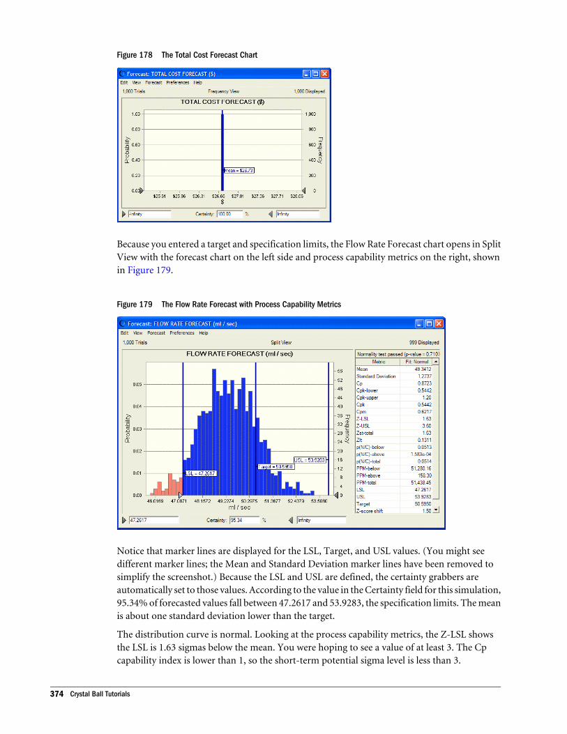
Figure 178 The Total Cost Forecast Chart
Because you entered a target and specification limits, the Flow Rate Forecast chart opens in SplitView with the forecast chart on the left side and process capability metrics on the right, shownin Figure 179.
Figure 179 The Flow Rate Forecast with Process Capability Metrics
Notice that marker lines are displayed for the LSL, Target, and USL values. (You might seedifferent marker lines; the Mean and Standard Deviation marker lines have been removed tosimplify the screenshot.) Because the LSL and USL are defined, the certainty grabbers areautomatically set to those values. According to the value in the Certainty field for this simulation,95.34% of forecasted values fall between 47.2617 and 53.9283, the specification limits. The meanis about one standard deviation lower than the target.
The distribution curve is normal. Looking at the process capability metrics, the Z-LSL showsthe LSL is 1.63 sigmas below the mean. You were hoping to see a value of at least 3. The Cpcapability index is lower than 1, so the short-term potential sigma level is less than 3.
374 Crystal Ball Tutorials
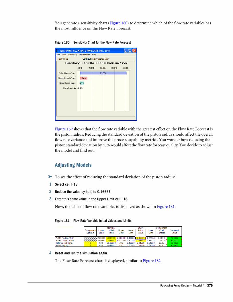
You generate a sensitivity chart (Figure 180) to determine which of the flow rate variables hasthe most influence on the Flow Rate Forecast.
Figure 180 Sensitivity Chart for the Flow Rate Forecast
Figure 169 shows that the flow rate variable with the greatest effect on the Flow Rate Forecast isthe piston radius. Reducing the standard deviation of the piston radius should affect the overallflow rate variance and improve the process capability metrics. You wonder how reducing thepiston standard deviation by 50% would affect the flow rate forecast quality. You decide to adjustthe model and find out.
Adjusting Models
ä To see the effect of reducing the standard deviation of the piston radius:
1 Select cell H18.
2 Reduce the value by half, to 0.16667.
3 Enter this same value in the Upper Limit cell, I18.
Now, the table of flow rate variables is displayed as shown in Figure 181.
Figure 181 Flow Rate Variable Initial Values and Limits
4 Reset and run the simulation again.
The Flow Rate Forecast chart is displayed, similar to Figure 182.
Packaging Pump Design — Tutorial 4 375
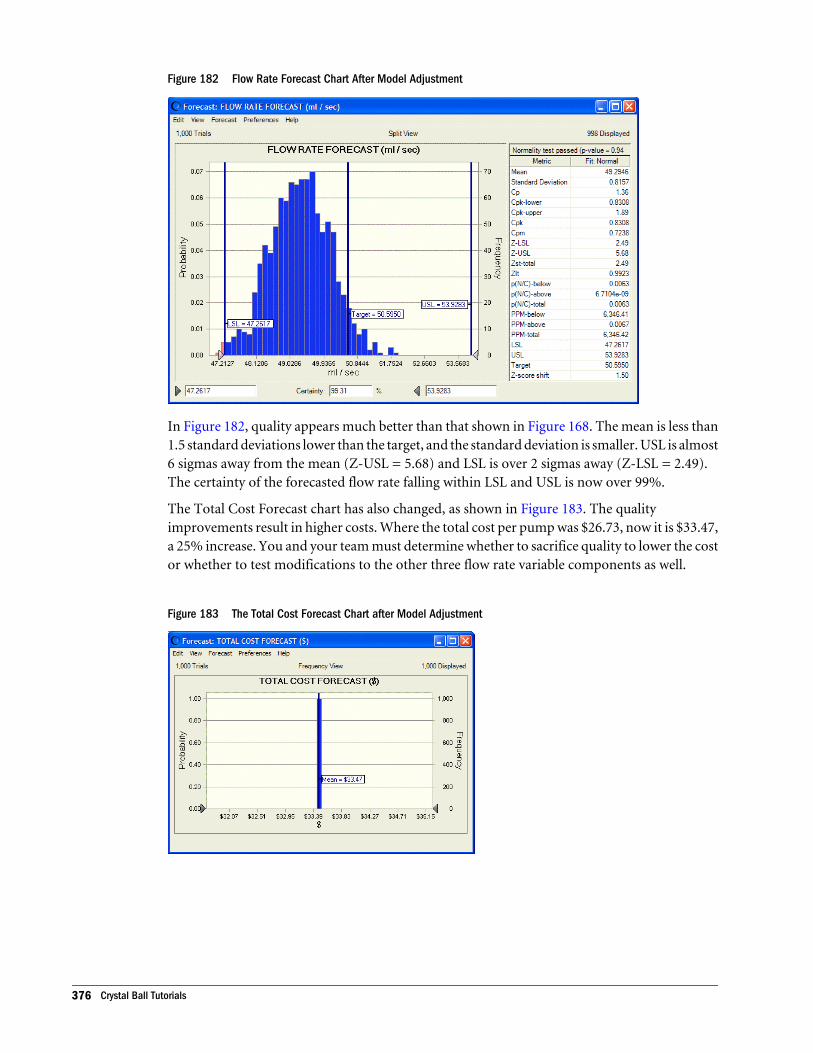
Figure 182 Flow Rate Forecast Chart After Model Adjustment
In Figure 182, quality appears much better than that shown in Figure 168. The mean is less than1.5 standard deviations lower than the target, and the standard deviation is smaller. USL is almost6 sigmas away from the mean (Z-USL = 5.68) and LSL is over 2 sigmas away (Z-LSL = 2.49).The certainty of the forecasted flow rate falling within LSL and USL is now over 99%.
The Total Cost Forecast chart has also changed, as shown in Figure 183. The qualityimprovements result in higher costs. Where the total cost per pump was $26.73, now it is $33.47,a 25% increase. You and your team must determine whether to sacrifice quality to lower the costor whether to test modifications to the other three flow rate variable components as well.
Figure 183 The Total Cost Forecast Chart after Model Adjustment
376 Crystal Ball Tutorials
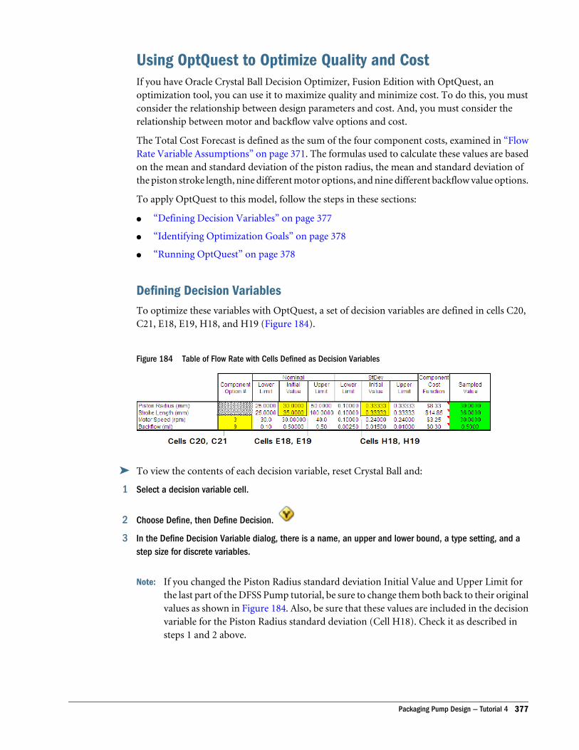
Using OptQuest to Optimize Quality and CostIf you have Oracle Crystal Ball Decision Optimizer, Fusion Edition with OptQuest, anoptimization tool, you can use it to maximize quality and minimize cost. To do this, you mustconsider the relationship between design parameters and cost. And, you must consider therelationship between motor and backflow valve options and cost.
The Total Cost Forecast is defined as the sum of the four component costs, examined in “FlowRate Variable Assumptions” on page 371. The formulas used to calculate these values are basedon the mean and standard deviation of the piston radius, the mean and standard deviation ofthe piston stroke length, nine different motor options, and nine different backflow value options.
To apply OptQuest to this model, follow the steps in these sections:
l “Defining Decision Variables” on page 377
l “Identifying Optimization Goals” on page 378
l “Running OptQuest” on page 378
Defining Decision VariablesTo optimize these variables with OptQuest, a set of decision variables are defined in cells C20,C21, E18, E19, H18, and H19 (Figure 184).
Figure 184 Table of Flow Rate with Cells Defined as Decision Variables
ä To view the contents of each decision variable, reset Crystal Ball and:
1 Select a decision variable cell.
2 Choose Define, then Define Decision.
3 In the Define Decision Variable dialog, there is a name, an upper and lower bound, a type setting, and astep size for discrete variables.
Note: If you changed the Piston Radius standard deviation Initial Value and Upper Limit forthe last part of the DFSS Pump tutorial, be sure to change them both back to their originalvalues as shown in Figure 184. Also, be sure that these values are included in the decisionvariable for the Piston Radius standard deviation (Cell H18). Check it as described insteps 1 and 2 above.
Packaging Pump Design — Tutorial 4 377
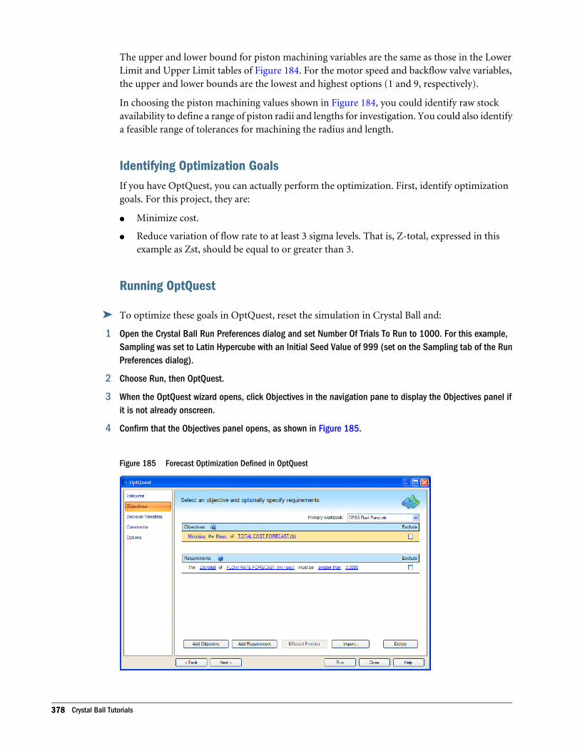
The upper and lower bound for piston machining variables are the same as those in the LowerLimit and Upper Limit tables of Figure 184. For the motor speed and backflow valve variables,the upper and lower bounds are the lowest and highest options (1 and 9, respectively).
In choosing the piston machining values shown in Figure 184, you could identify raw stockavailability to define a range of piston radii and lengths for investigation. You could also identifya feasible range of tolerances for machining the radius and length.
Identifying Optimization GoalsIf you have OptQuest, you can actually perform the optimization. First, identify optimizationgoals. For this project, they are:
l Minimize cost.
l Reduce variation of flow rate to at least 3 sigma levels. That is, Z-total, expressed in thisexample as Zst, should be equal to or greater than 3.
Running OptQuest
ä To optimize these goals in OptQuest, reset the simulation in Crystal Ball and:
1 Open the Crystal Ball Run Preferences dialog and set Number Of Trials To Run to 1000. For this example,Sampling was set to Latin Hypercube with an Initial Seed Value of 999 (set on the Sampling tab of the RunPreferences dialog).
2 Choose Run, then OptQuest.
3 When the OptQuest wizard opens, click Objectives in the navigation pane to display the Objectives panel ifit is not already onscreen.
4 Confirm that the Objectives panel opens, as shown in Figure 185.
Figure 185 Forecast Optimization Defined in OptQuest
378 Crystal Ball Tutorials
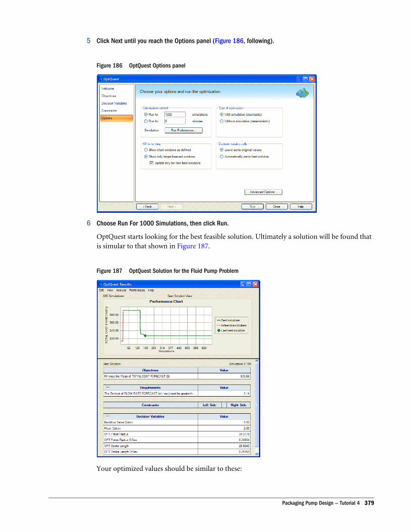
5 Click Next until you reach the Options panel (Figure 186, following).
Figure 186 OptQuest Options panel
6 Choose Run For 1000 Simulations, then click Run.
OptQuest starts looking for the best feasible solution. Ultimately a solution will be found thatis simular to that shown in Figure 187.
Figure 187 OptQuest Solution for the Fluid Pump Problem
Your optimized values should be similar to these:
Packaging Pump Design — Tutorial 4 379
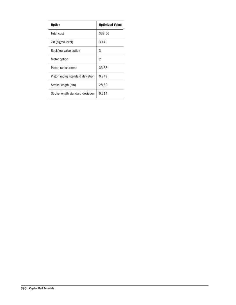
Option Optimized Value
Total cost $33.66
Zst (sigma level) 3.14
Backflow valve option 3
Motor option 2
Piston radius (mm) 33.38
Piston radius standard deviation 0.249
Stroke length (cm) 28.60
Stroke length standard deviation 0.214
380 Crystal Ball Tutorials
EUsing the Process Capability
Features
In This Appendix
Introduction... . . . . . . . . . . . . . . . . . . . . . . . . . . . . . . . . . . . . . . . . . . . . . . . . . . . . . . . . . . . . . . . . . . . . . . . . . . . . . . . . . . . . . . . . . . . . . . . . . . . . . . . . . . . . . . . . . . . . 381
About Crystal Ball’s Process Capability Features ... . . . . . . . . . . . . . . . . . . . . . . . . . . . . . . . . . . . . . . . . . . . . . . . . . . . . . . . . . . . . . . . . . . . . . . . . . . 381
About Quality Improvement Methodologies ... . . . . . . . . . . . . . . . . . . . . . . . . . . . . . . . . . . . . . . . . . . . . . . . . . . . . . . . . . . . . . . . . . . . . . . . . . . . . . . . . 382
How Crystal Ball Supports Quality .. . . . . . . . . . . . . . . . . . . . . . . . . . . . . . . . . . . . . . . . . . . . . . . . . . . . . . . . . . . . . . . . . . . . . . . . . . . . . . . . . . . . . . . . . . . . . 384
Working Through Process Capability Tutorials .. . . . . . . . . . . . . . . . . . . . . . . . . . . . . . . . . . . . . . . . . . . . . . . . . . . . . . . . . . . . . . . . . . . . . . . . . . . . . . . . 386
Preparing to Use Process Capability Features... . . . . . . . . . . . . . . . . . . . . . . . . . . . . . . . . . . . . . . . . . . . . . . . . . . . . . . . . . . . . . . . . . . . . . . . . . . . . . . 386
Analyzing Process Capability Results .. . . . . . . . . . . . . . . . . . . . . . . . . . . . . . . . . . . . . . . . . . . . . . . . . . . . . . . . . . . . . . . . . . . . . . . . . . . . . . . . . . . . . . . . . 388
Capability Metrics List . . . . . . . . . . . . . . . . . . . . . . . . . . . . . . . . . . . . . . . . . . . . . . . . . . . . . . . . . . . . . . . . . . . . . . . . . . . . . . . . . . . . . . . . . . . . . . . . . . . . . . . . . . . 393
IntroductionThis appendix describes Crystal Ball’s process capability features, which support qualityimprovement methodologies such as Six Sigma, DFSS (Design for Six Sigma), and Leanprinciples.
The following sections introduce the process capability features and describe how to use them:
l “About Crystal Ball’s Process Capability Features” on page 381
l “Preparing to Use Process Capability Features” on page 386
l “Analyzing Process Capability Results” on page 388
l “Capability Metrics List” on page 393
About Crystal Ball’s Process Capability FeaturesUse the Statistics tab of the Run Preferences dialog to activate the process capability features.After they are activated, you can:
l Add upper and lower specification limits and target values to forecast definitions (“SettingSpecification Limits and Targets” on page 387).
l Display the Capability Metrics view in the forecast window, in addition to the basicFrequency, Cumulative Frequency, Reverse Cumulative Frequency, Statistics, andPercentiles views (“Viewing Capability Metrics” on page 388).
Introduction 381
l Use Crystal Ball’s Split View feature to display the Capability Metrics view to the right ofone of the forecast chart views (“Viewing Forecast Charts and Capability Metrics Together”on page 389). This is the default.
l View marker lines for specification limits and the target value on forecast charts (“ViewingLSL, USL, and Target Marker Lines” on page 391).
l Extract capability metrics to a worksheet using Analyze, then Extract Data or the AutoExtract forecast preferences (“Extracting Capability Metrics” on page 391).
l Include capability metrics in reports (“Including Capability Metrics in Reports” on page392).
l Include several capability metrics in OptQuest, if you have a license for it, and specify themas objectives or requirements.
l Access capability metrics in the Crystal Ball Developer Kit using these calls: CB.SetFore,CB.GetFore, CB.DefineForeND, CB.SetView, CB.GetForeStat, CB.RunPrefsND,CB.GetRunPrefs, CB.CreateRptND, and CB.ExtractDataND (see the Crystal Ball DeveloperKit User's Guide for more information)
Several of these calls have equivalent spreadsheet functions and can be used in worksheet cellsinstead of VBA macros.
The following sections summarize process capability initiatives for quality improvement anddescribe how Crystal Ball's process capability features support those initiatives:
l “About Quality Improvement Methodologies” on page 382
l “How Crystal Ball Supports Quality” on page 384
l “Working Through Process Capability Tutorials” on page 386
About Quality Improvement MethodologiesStarting about 1975, competitive pressures on manufacturers encouraged them to discover newquality methodologies. Leading companies developed a variety of techniques to save costs andtime by improving processes, designing more effectively, and increasing the value of productmodifications.
Some of the most successful methodologies have been Six Sigma, Design for Six Sigma (DFSS),Lean principles, and similar tools for quality improvement. The following sections summarizeseveral of these:
l “Methodologies for Improving Processes — Six Sigma” on page 382
l “Methodologies for Improving Design — DFSS” on page 383
l “Methodologies for Adding Value — Lean Principles” on page 383
Methodologies for Improving Processes — Six SigmaBroken processes reduce quality in a variety of organizations, from banking to manufacturingto healthcare, and more. In the United States, Six Sigma is probably the best known process
382 Using the Process Capability Features
improvement methodology, although other techniques have similar goals and effectiveness inthe field.
Six Sigma is a methodology for improving processes to achieve any or all of the following goals:
l Reducing the defect rate to 3.4 per million (outside the range of 6 standard deviations aboveand below the mean)
l Creating improvements of 70% or better
l Using the Define-Measure-Analyze-Improve-Control methodology of informationgathering, analysis, and action
l Producing rapid improvement of an organization’s financial "bottom-line."
Six Sigma methodology is data-driven and focuses on the relationship between system inputsand outputs, both of which can vary. The inputs, or independent variables, are symbolized byX; the outputs, or dependent variables, are symbolized by Y. The goal of a Six Sigma program isto yield maximum quality and minimum variation in Y by controlling variation in all the Xvariables, the factors that influence it.
Six Sigma teams talk about the "hidden factory" of workers behind the scenes who rework defectsand perform other extra tasks to make up for broken processes. Six Sigma programs achievetheir goals by discovering the hidden factory in their organization and releasing its workers formore productive tasks.
Methodologies for Improving Design — DFSSDesign for Six Sigma (DFSS) developed following the success of Six Sigma and other processimprovement methodologies. If a similar multi-phase improvment technique could be appliedto design, costs and time could be saved by eliminating waste and unnecessary prototyping.Successful designs could move to production quicker, reducing costs and increasing anorganization’s competitive edge. DFSS proved to be a successful tool for improving design in avariety of settings. The five phases of DFSS are Define, Measure, Analyze, Design, and Verify(DMADV).
The ultimate mission of DFSS is to address general Six Sigma goals of meeting customer needswhile minimizing variation and to accomplish this as early in the development cycle as possible.
Methodologies for Adding Value — Lean PrinciplesThe Lean approach to quality focuses on eliminating waste, improving efficiency, and increasingvalue. Lean techniques seek to increase value by improving the flow of value stream activitiesand reducing waste. Other Lean principles include just-in-time delivery driven by customer pull— not push — and a constant, incremental search for perfection (sometimes called kaizen).
Lean practitioners use value stream mapping to identify process steps with the greatest impacton the overall product. Then, Lean projects are created to improve those processes. The "hiddenfactory" is a major target for Lean programs, as practitioners seek to eliminate rework and scrap.Lean principles are often used with statistical methodologies such as Six Sigma.
About Quality Improvement Methodologies 383
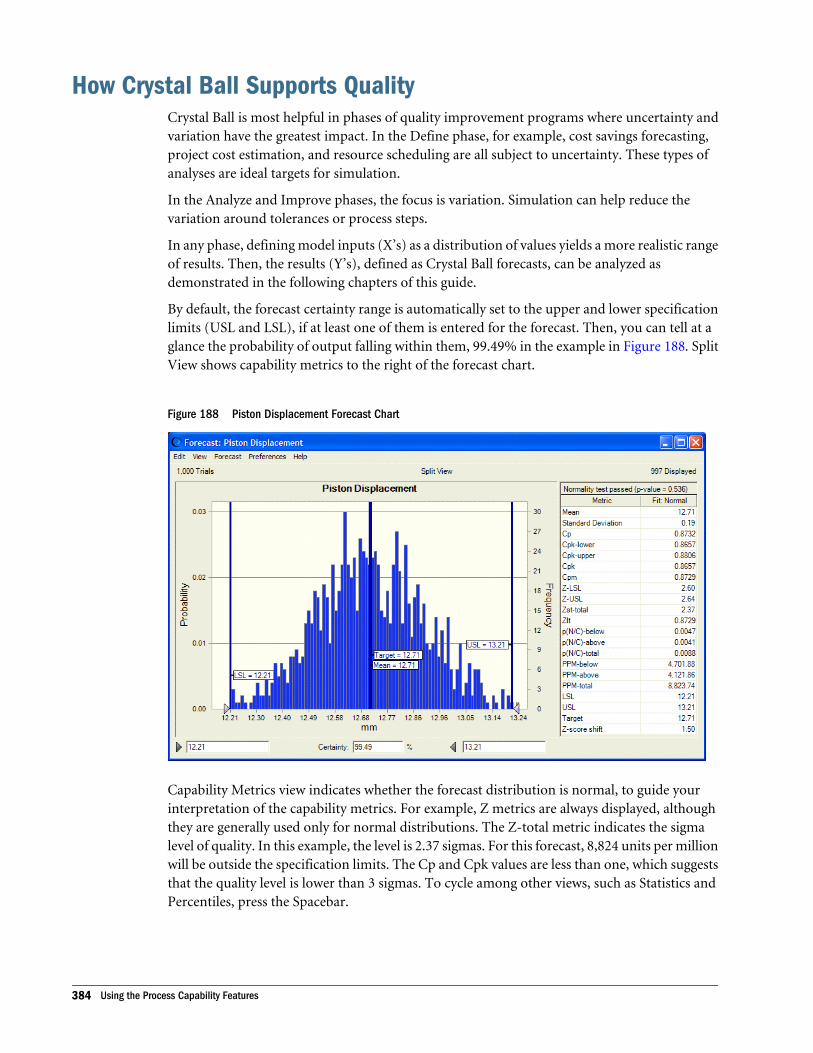
How Crystal Ball Supports QualityCrystal Ball is most helpful in phases of quality improvement programs where uncertainty andvariation have the greatest impact. In the Define phase, for example, cost savings forecasting,project cost estimation, and resource scheduling are all subject to uncertainty. These types ofanalyses are ideal targets for simulation.
In the Analyze and Improve phases, the focus is variation. Simulation can help reduce thevariation around tolerances or process steps.
In any phase, defining model inputs (X’s) as a distribution of values yields a more realistic rangeof results. Then, the results (Y’s), defined as Crystal Ball forecasts, can be analyzed asdemonstrated in the following chapters of this guide.
By default, the forecast certainty range is automatically set to the upper and lower specificationlimits (USL and LSL), if at least one of them is entered for the forecast. Then, you can tell at aglance the probability of output falling within them, 99.49% in the example in Figure 188. SplitView shows capability metrics to the right of the forecast chart.
Figure 188 Piston Displacement Forecast Chart
Capability Metrics view indicates whether the forecast distribution is normal, to guide yourinterpretation of the capability metrics. For example, Z metrics are always displayed, althoughthey are generally used only for normal distributions. The Z-total metric indicates the sigmalevel of quality. In this example, the level is 2.37 sigmas. For this forecast, 8,824 units per millionwill be outside the specification limits. The Cp and Cpk values are less than one, which suggeststhat the quality level is lower than 3 sigmas. To cycle among other views, such as Statistics andPercentiles, press the Spacebar.
384 Using the Process Capability Features
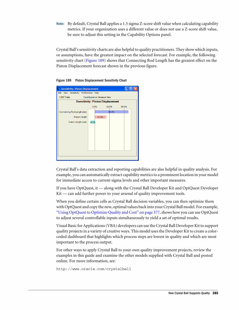
Note: By default, Crystal Ball applies a 1.5 sigma Z-score shift value when calculating capabilitymetrics. If your organization uses a different value or does not use a Z-score shift value,be sure to adjust this setting in the Capability Options panel.
Crystal Ball’s sensitivity charts are also helpful to quality practitioners. They show which inputs,or assumptions, have the greatest impact on the selected forecast. For example, the followingsensitivity chart (Figure 189) shows that Connecting Rod Length has the greatest effect on thePiston Displacement forecast shown in the previous figure.
Figure 189 Piston Displacement Sensitivity Chart
Crystal Ball’s data extraction and reporting capabilities are also helpful in quality analysis. Forexample, you can automatically extract capability metrics to a prominent location in your modelfor immediate access to current sigma levels and other important measures.
If you have OptQuest, it — along with the Crystal Ball Developer Kit and OptQuest DeveloperKit — can add further power to your arsenal of quality improvement tools.
When you define certain cells as Crystal Ball decision variables, you can then optimize themwith OptQuest and copy the new, optimal values back into your Crystal Ball model. For example,“Using OptQuest to Optimize Quality and Cost” on page 377, shows how you can use OptQuestto adjust several controllable inputs simultaneously to yield a set of optimal results.
Visual Basic for Applications (VBA) developers can use the Crystal Ball Developer Kit to supportquality projects in a variety of creative ways. This model uses the Developer Kit to create a color-coded dashboard that highlights which process steps are lowest in quality and which are mostimportant to the process output.
For other ways to apply Crystal Ball to your own quality improvement projects, review theexamples in this guide and examine the other models supplied with Crystal Ball and postedonline. For more information, see:
http://www.oracle.com/crystalball
How Crystal Ball Supports Quality 385
Working Through Process Capability TutorialsAs you learn about the Crystal Ball process capability features, consider working through thefollowing tutorials:
l “Improving Process Quality — Tutorial 3” on page 352
l “Packaging Pump Design — Tutorial 4” on page 366
They show how the process capability features can be used within quality improvementmethodologies to simplify quality initiatives in a variety of settings.
Preparing to Use Process Capability FeaturesBefore you can use the process capability features, you must activate them, set options, and enterlimits and target values for at least one forecast. The following sections describe these procedures:
l “Activating the Process Capability Features” on page 386
l “Setting Capability Calculation Options” on page 386
l “Setting Specification Limits and Targets” on page 387
Activating the Process Capability Features
ä To activate Crystal Ball’s process capability features:
1 Choose Run, then Run Preferences to display the Run Preferences dialog.
2 Click the Statistics tab.
3 Check Calculate Capability Metrics.
4 Click the Options button to set the capability calculation options, described in the next section.
5 Click OK when setting changes are complete.
Setting Capability Calculation OptionsAfter you activate the process capability features, you can set a variety of options to furthercustomize these features for your situation.
ä To set the process capability options:
1 Display the Statistics tab of the Run Preferences dialog.
2 Click the Options button as described in step 5 of the previous section.
The Capability Options panel opens.
3 Indicate whether metrics should use short-term or long-term formulas, depending on the time-span of yourmodel.
4 Optionally, specify a Z-score shift value to be used in long-term formulas.
386 Using the Process Capability Features
You can specify a value from 0 to 100.
The default is 1.5. If don’t want to use a Z-score shift value, enter 0 in the box or delete thecurrent value and leave it empty.
5 Indicate whether metrics should be calculated from a fitted distribution or directly from the forecast values(“Calculation Method” on page 387).
6 When settings are complete, click OK.
Calculation MethodBy default, Crystal Ball tries to fit a normal distribution to the forecast values. You can enter asignificance level to specify the threshold below which the assumption of normality is rejected.The default level of 0.05 translates into a 95% confidence that a rejection of normality will becorrect. Other significance levels typically used are 0.01, 0.025, and 0.1, which translate into 99%,97.5%, and 90% confidences, respectively.
If normality is rejected, Crystal Ball will then either calculate the metrics directly from the forecastvalues (the default) or, if you choose, perform a best fit to select the most appropriate continuousprobability distribution from which to calculate the metrics.
The normality test and non-normal best fit (if normality is rejected) use the goodness-of-fit testand distribution selection that is set in the Forecast Window tab of the Forecast Preferencesdialog (opened by choosing Preferences, then Forecast in the forecast window).
Before you choose to calculate from the best fitting distribution if the distribution is not normal,consider that:
l You are not guaranteed of attaining a good fit to the forecast values, and
l The fitting process might take a long time depending on how many simulation trials youare running.
Note: In unusual circumstances, it is possible for the normality test to fail and the best fittingdistribution still be a normal distribution, or for the normality test to pass and thebest fitting distribution be non-normal.
Alternatively, you can choose the second main setting, Calculate Metrics From Forecast Values,to bypass the normality test and always calculate the metrics directly from the forecast data.
Setting Specification Limits and TargetsThe capability metrics only display if you specify either an upper or lower specification limit (orboth) for the forecast. You can also specify an optional target.
ä To specify these limits:
1 Either define a new forecast or select an existing forecast and choose Define, then Define Forecast.
The Define Forecast dialog opens. With process capability features activated, it includes Name,Units, LSL, USL, and Target fields..
Preparing to Use Process Capability Features 387
2 Enter specification limits and target values for this forecast into the appropriate fields.
LSL = lower specification limit, USL = upper specification limit, and Target = target value forthis forecast. If you prefer, you can enter cell references by typing or browsing.
All of these fields are optional, but Crystal Ball only calculates capability metrics if a value isentered for one or both of the specification limits.
3 To set forecast preferences at the same time, click the More button, , to the right of the Name field.
4 When all settings are complete, click OK.
For information about the relationship of the LSL and USL to the certainty range, see “ViewingLSL, USL, and Target Marker Lines” on page 391
Analyzing Process Capability ResultsWhen capability metrics have been activated and appropriate information entered, run a CrystalBall simulation as usual. Then, you can perform the following capability analyses:
l “Viewing Capability Metrics” on page 388
l “Extracting Capability Metrics” on page 391
l “Including Capability Metrics in Reports” on page 392
Viewing Capability MetricsAfter you have defined a forecast with at least one specification limit (and, optionally, a target),you can run a simulation and display capability metrics for the forecast.
ä To display capability metrics:
1 Define a forecast with LSL, USL, and Target values as described in “Setting Specification Limits and Targets”on page 387.
2 Run the simulation and display the chart for that forecast.
3 In the forecast window, choose View, then Capability Metrics.
A table of metrics opens, similar to Figure 190.
388 Using the Process Capability Features
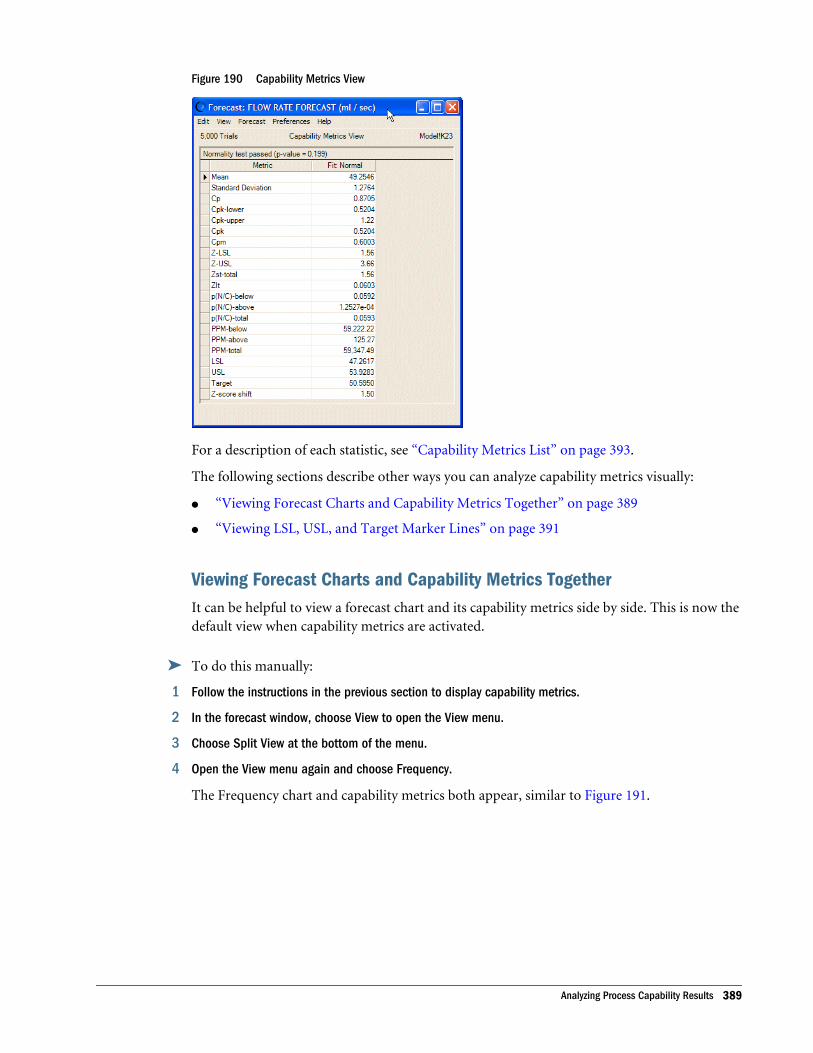
Figure 190 Capability Metrics View
For a description of each statistic, see “Capability Metrics List” on page 393.
The following sections describe other ways you can analyze capability metrics visually:
l “Viewing Forecast Charts and Capability Metrics Together” on page 389
l “Viewing LSL, USL, and Target Marker Lines” on page 391
Viewing Forecast Charts and Capability Metrics TogetherIt can be helpful to view a forecast chart and its capability metrics side by side. This is now thedefault view when capability metrics are activated.
ä To do this manually:
1 Follow the instructions in the previous section to display capability metrics.
2 In the forecast window, choose View to open the View menu.
3 Choose Split View at the bottom of the menu.
4 Open the View menu again and choose Frequency.
The Frequency chart and capability metrics both appear, similar to Figure 191.
Analyzing Process Capability Results 389
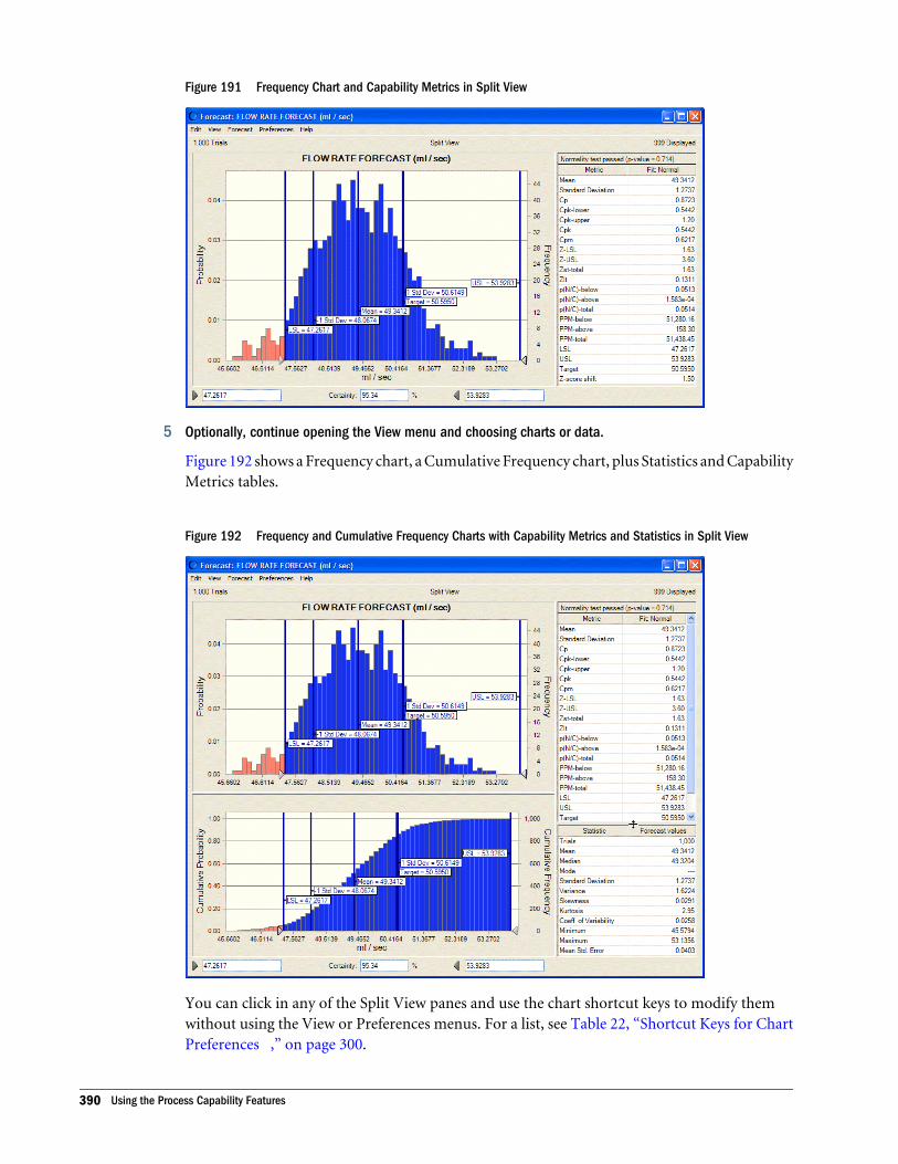
Figure 191 Frequency Chart and Capability Metrics in Split View
5 Optionally, continue opening the View menu and choosing charts or data.
Figure 192 shows a Frequency chart, a Cumulative Frequency chart, plus Statistics and CapabilityMetrics tables.
Figure 192 Frequency and Cumulative Frequency Charts with Capability Metrics and Statistics in Split View
You can click in any of the Split View panes and use the chart shortcut keys to modify themwithout using the View or Preferences menus. For a list, see Table 22, “Shortcut Keys for ChartPreferences ,” on page 300.
390 Using the Process Capability Features
You can also resize the chart window and drag the horizontal and vertical pane splitters to resizeeach part of the Split View window.
Viewing LSL, USL, and Target Marker LinesBy default, after you add specification limits and a target to a forecast, markers for these valuesare displayed on the forecast chart. For an example, see Figure 192.
Notice that the certainty range on the forecast chart changes to match the LSL and USL values.The certainty indicates the probability of falling within those specification limits. To show thecertainty of different values, type them into the Minimum and Maximum fields or click thecertainty grabbers and drag them to a new position.
ä To add specification limit and target marker lines manually or to remove them:
1 Choose Preferences, then Chart Preferences in a forecast chart window, or double-click the chart.
2 Click the Chart Type tab in the Chart Preferences dialog.
3 Scroll down to the bottom of the Marker Lines list.
4 Be sure LSL, USL, Target is checked to display the specification limit and target marker lines on that forecastchart.
To hide the markers, uncheck LSL, USL, Target.
5 When all settings are complete, click OK.
Notice that you can display the mean and other marker lines in addition to the specificationlimit and target markers.
Extracting Capability MetricsYou can extract capability metrics automatically or manually, as described in the followingsections:
l “Extracting Capability Metrics Automatically” on page 391
l “Extracting Capability Metrics Manually” on page 392
Extracting Capability Metrics Automatically
ä You can automatically extract capability metrics whenever a simulation runs. To extract metricsautomatically:
1 In a forecast window, choose Preferences, then Forecast and display the Auto Extract tab of the ForecastPreferences dialog.
2 Check Extract Forecast Statistics Automatically... and scroll down to the bottom of the data selection list.
3 Check Capability Metrics, enter a Starting Cell, and then click OK.
Now, when you run a simulation, capability metrics are written to the specified area of yourworksheet, along with any other data you have requested.
Analyzing Process Capability Results 391
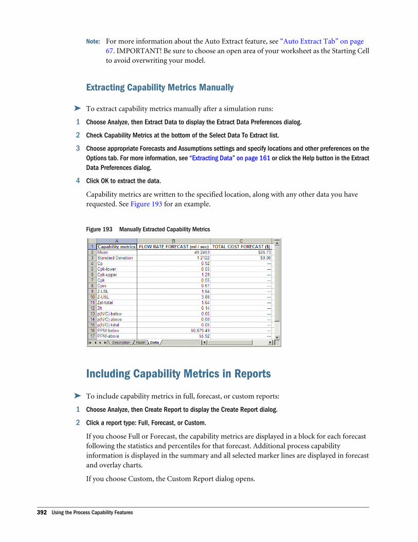
Note: For more information about the Auto Extract feature, see “Auto Extract Tab” on page67. IMPORTANT! Be sure to choose an open area of your worksheet as the Starting Cellto avoid overwriting your model.
Extracting Capability Metrics Manually
ä To extract capability metrics manually after a simulation runs:
1 Choose Analyze, then Extract Data to display the Extract Data Preferences dialog.
2 Check Capability Metrics at the bottom of the Select Data To Extract list.
3 Choose appropriate Forecasts and Assumptions settings and specify locations and other preferences on theOptions tab. For more information, see “Extracting Data” on page 161 or click the Help button in the ExtractData Preferences dialog.
4 Click OK to extract the data.
Capability metrics are written to the specified location, along with any other data you haverequested. See Figure 193 for an example.
Figure 193 Manually Extracted Capability Metrics
Including Capability Metrics in Reports
ä To include capability metrics in full, forecast, or custom reports:
1 Choose Analyze, then Create Report to display the Create Report dialog.
2 Click a report type: Full, Forecast, or Custom.
If you choose Full or Forecast, the capability metrics are displayed in a block for each forecastfollowing the statistics and percentiles for that forecast. Additional process capabilityinformation is displayed in the summary and all selected marker lines are displayed in forecastand overlay charts.
If you choose Custom, the Custom Report dialog opens.
392 Using the Process Capability Features
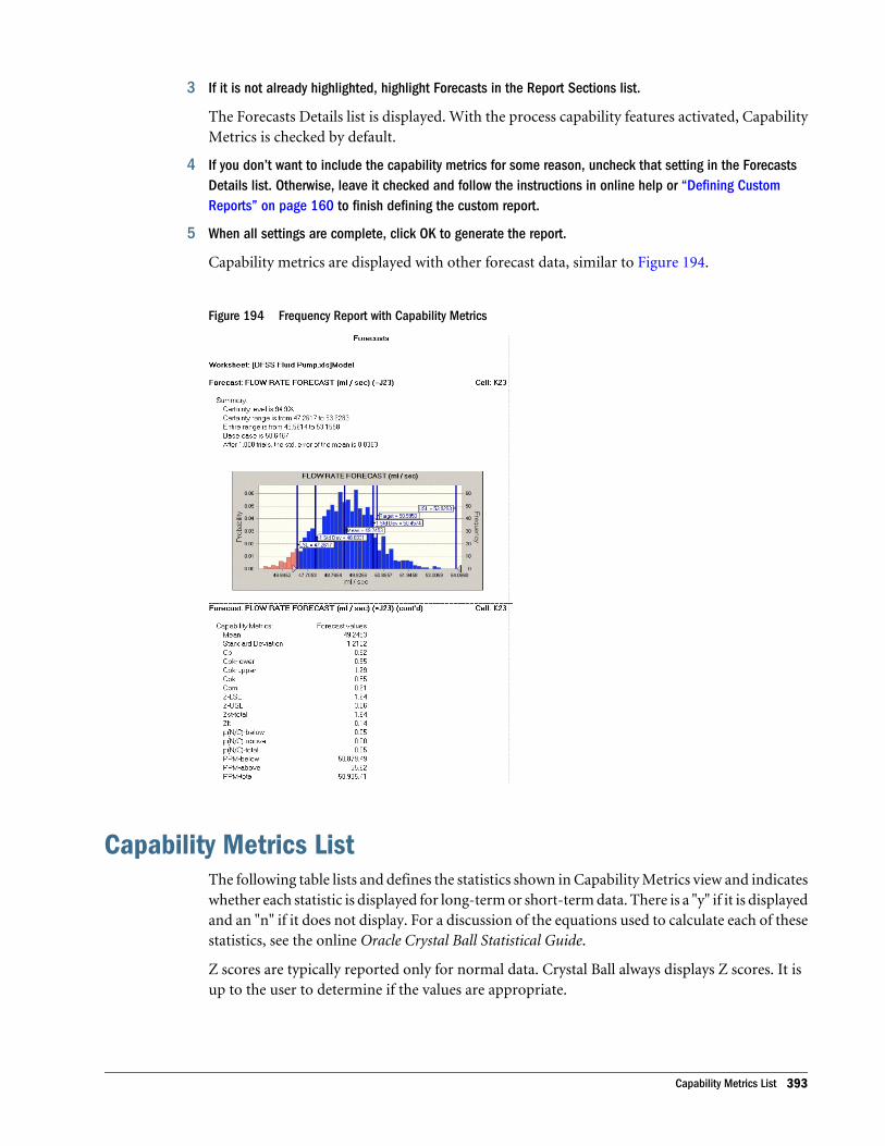
3 If it is not already highlighted, highlight Forecasts in the Report Sections list.
The Forecasts Details list is displayed. With the process capability features activated, CapabilityMetrics is checked by default.
4 If you don’t want to include the capability metrics for some reason, uncheck that setting in the ForecastsDetails list. Otherwise, leave it checked and follow the instructions in online help or “Defining CustomReports” on page 160 to finish defining the custom report.
5 When all settings are complete, click OK to generate the report.
Capability metrics are displayed with other forecast data, similar to Figure 194.
Figure 194 Frequency Report with Capability Metrics
Capability Metrics ListThe following table lists and defines the statistics shown in Capability Metrics view and indicateswhether each statistic is displayed for long-term or short-term data. There is a "y" if it is displayedand an "n" if it does not display. For a discussion of the equations used to calculate each of thesestatistics, see the online Oracle Crystal Ball Statistical Guide.
Z scores are typically reported only for normal data. Crystal Ball always displays Z scores. It isup to the user to determine if the values are appropriate.
Capability Metrics List 393
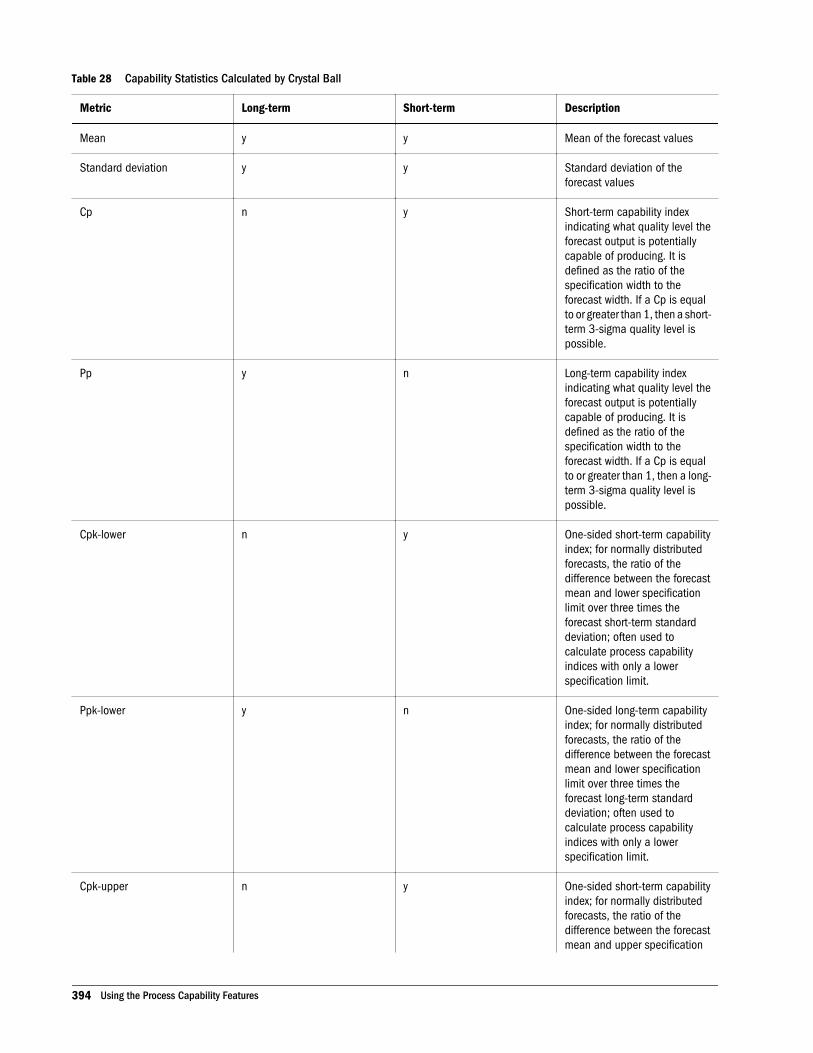
Table 28 Capability Statistics Calculated by Crystal Ball
Metric Long-term Short-term Description
Mean y y Mean of the forecast values
Standard deviation y y Standard deviation of theforecast values
Cp n y Short-term capability indexindicating what quality level theforecast output is potentiallycapable of producing. It isdefined as the ratio of thespecification width to theforecast width. If a Cp is equalto or greater than 1, then a short-term 3-sigma quality level ispossible.
Pp y n Long-term capability indexindicating what quality level theforecast output is potentiallycapable of producing. It isdefined as the ratio of thespecification width to theforecast width. If a Cp is equalto or greater than 1, then a long-term 3-sigma quality level ispossible.
Cpk-lower n y One-sided short-term capabilityindex; for normally distributedforecasts, the ratio of thedifference between the forecastmean and lower specificationlimit over three times theforecast short-term standarddeviation; often used tocalculate process capabilityindices with only a lowerspecification limit.
Ppk-lower y n One-sided long-term capabilityindex; for normally distributedforecasts, the ratio of thedifference between the forecastmean and lower specificationlimit over three times theforecast long-term standarddeviation; often used tocalculate process capabilityindices with only a lowerspecification limit.
Cpk-upper n y One-sided short-term capabilityindex; for normally distributedforecasts, the ratio of thedifference between the forecastmean and upper specification
394 Using the Process Capability Features
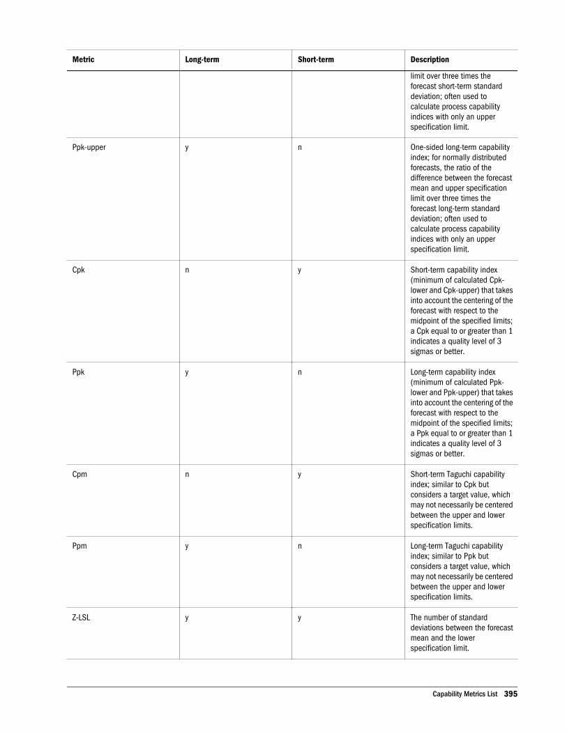
Metric Long-term Short-term Description
limit over three times theforecast short-term standarddeviation; often used tocalculate process capabilityindices with only an upperspecification limit.
Ppk-upper y n One-sided long-term capabilityindex; for normally distributedforecasts, the ratio of thedifference between the forecastmean and upper specificationlimit over three times theforecast long-term standarddeviation; often used tocalculate process capabilityindices with only an upperspecification limit.
Cpk n y Short-term capability index(minimum of calculated Cpk-lower and Cpk-upper) that takesinto account the centering of theforecast with respect to themidpoint of the specified limits;a Cpk equal to or greater than 1indicates a quality level of 3sigmas or better.
Ppk y n Long-term capability index(minimum of calculated Ppk-lower and Ppk-upper) that takesinto account the centering of theforecast with respect to themidpoint of the specified limits;a Ppk equal to or greater than 1indicates a quality level of 3sigmas or better.
Cpm n y Short-term Taguchi capabilityindex; similar to Cpk butconsiders a target value, whichmay not necessarily be centeredbetween the upper and lowerspecification limits.
Ppm y n Long-term Taguchi capabilityindex; similar to Ppk butconsiders a target value, whichmay not necessarily be centeredbetween the upper and lowerspecification limits.
Z-LSL y y The number of standarddeviations between the forecastmean and the lowerspecification limit.
Capability Metrics List 395
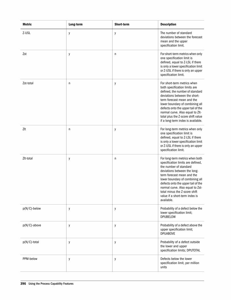
Metric Long-term Short-term Description
Z-USL y y The number of standarddeviations between the forecastmean and the upperspecification limit.
Zst y n For short-term metrics when onlyone specification limit isdefined, equal to Z-LSL if thereis only a lower specification limitor Z-USL if there is only an upperspecification limit.
Zst-total n y For short-term metrics whenboth specification limits aredefined, the number of standarddeviations between the short-term forecast mean and thelower boundary of combining alldefects onto the upper tail of thenormal curve. Also equal to Zlt-total plus the Z-score shift valueif a long-term index is available.
Zlt n y For long-term metrics when onlyone specification limit isdefined, equal to Z-LSL if thereis only a lower specification limitor Z-USL if there is only an upperspecification limit.
Zlt-total y n For long-term metrics when bothspecification limits are defined,the number of standarddeviations between the long-term forecast mean and thelower boundary of combining alldefects onto the upper tail of thenormal curve. Also equal to Zst-total minus the Z-score shiftvalue if a short-term index isavailable.
p(N/C)-below y y Probability of a defect below thelower specification limit;DPUBELOW
p(N/C)-above y y Probability of a defect above theupper specification limit;DPUABOVE
p(N/C)-total y y Probability of a defect outsidethe lower and upperspecification limits; DPUTOTAL
PPM-below y y Defects below the lowerspecification limit, per millionunits
396 Using the Process Capability Features
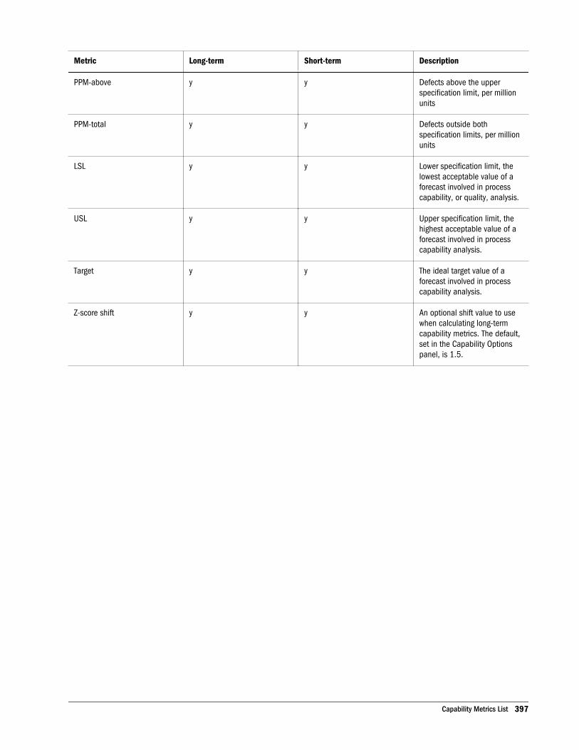
Metric Long-term Short-term Description
PPM-above y y Defects above the upperspecification limit, per millionunits
PPM-total y y Defects outside bothspecification limits, per millionunits
LSL y y Lower specification limit, thelowest acceptable value of aforecast involved in processcapability, or quality, analysis.
USL y y Upper specification limit, thehighest acceptable value of aforecast involved in processcapability analysis.
Target y y The ideal target value of aforecast involved in processcapability analysis.
Z-score shift y y An optional shift value to usewhen calculating long-termcapability metrics. The default,set in the Capability Optionspanel, is 1.5.
Capability Metrics List 397

398 Using the Process Capability Features
FBibliography
In This Appendix
Bootstrap ... . . . . . . . . . . . . . . . . . . . . . . . . . . . . . . . . . . . . . . . . . . . . . . . . . . . . . . . . . . . . . . . . . . . . . . . . . . . . . . . . . . . . . . . . . . . . . . . . . . . . . . . . . . . . . . . . . . . . . . 399
Monte Carlo Simulation ... . . . . . . . . . . . . . . . . . . . . . . . . . . . . . . . . . . . . . . . . . . . . . . . . . . . . . . . . . . . . . . . . . . . . . . . . . . . . . . . . . . . . . . . . . . . . . . . . . . . . . . 399
Probability Theory and Statistics.. . . . . . . . . . . . . . . . . . . . . . . . . . . . . . . . . . . . . . . . . . . . . . . . . . . . . . . . . . . . . . . . . . . . . . . . . . . . . . . . . . . . . . . . . . . . . . . 400
Random Variate Generation Methods... . . . . . . . . . . . . . . . . . . . . . . . . . . . . . . . . . . . . . . . . . . . . . . . . . . . . . . . . . . . . . . . . . . . . . . . . . . . . . . . . . . . . . . . 400
Specific Distributions ... . . . . . . . . . . . . . . . . . . . . . . . . . . . . . . . . . . . . . . . . . . . . . . . . . . . . . . . . . . . . . . . . . . . . . . . . . . . . . . . . . . . . . . . . . . . . . . . . . . . . . . . . . 401
Tornado Charts and Sensitivity Analysis .. . . . . . . . . . . . . . . . . . . . . . . . . . . . . . . . . . . . . . . . . . . . . . . . . . . . . . . . . . . . . . . . . . . . . . . . . . . . . . . . . . . . . . 401
Two-Dimensional Simulation... . . . . . . . . . . . . . . . . . . . . . . . . . . . . . . . . . . . . . . . . . . . . . . . . . . . . . . . . . . . . . . . . . . . . . . . . . . . . . . . . . . . . . . . . . . . . . . . . . 402
Uncertainty Analysis .. . . . . . . . . . . . . . . . . . . . . . . . . . . . . . . . . . . . . . . . . . . . . . . . . . . . . . . . . . . . . . . . . . . . . . . . . . . . . . . . . . . . . . . . . . . . . . . . . . . . . . . . . . . . 402
Sequential Sampling with SIPs ... . . . . . . . . . . . . . . . . . . . . . . . . . . . . . . . . . . . . . . . . . . . . . . . . . . . . . . . . . . . . . . . . . . . . . . . . . . . . . . . . . . . . . . . . . . . . . . 402
BootstrapEfron, Bradley, and Robert J. Tibshirani. "An Introduction to the Bootstrap," Monographs onStatistics and Applied Probability, vol. 57. New York: Chapman and Hall, 1993.
Mooney, C. Z., and R.D. Duval. "Bootstrapping: A Nonparametric Approach to StatisticalInference," Sage University Paper Series on Quantitative Applications in the Social Sciences,series no. 07-095. Newbury Park, CA: Sage, 1993.
Monte Carlo SimulationBurmaster, D.E., and P.D. Anderson, "Principles of Good Practice for the Use of Monte CarloTechniques in Human Health and Ecological Risk Assessments," Risk Analysis 14(4): 477-481(1994).
Hammersley, J.M., and D.C. Handscomb. Monte Carlo Methods. New York: Chapman andHall, 1965.
Kalos, Malvin H., and Paula A. Whitlock. Monte Carlo Methods. New York: John Wiley & Sons,1986.
Morgan, Byron J.T. Elements of Simulation. Portland, ME: Chapman and Hall, 1984.
Rubinstein, Reuven Y. Simulation and the Monte Carlo Method. New York: John Wiley & Sons,1981.
Thommes, M.C. Proper Spreadsheet Design. Boston: Boyd and Fraser Publishing Co., 1992.
Bootstrap 399
Thompson, K.M., D.E. Burmaster, and E.A.C. Crouch. "Monte Carlo Techniques forQuantitative Uncertainty Analysis in Public Health Risk Assessments," Risk Analysis 12(1):53-63 (1992).
Yakowitz, Sidney J. Computational Probability and Simulation. Reading, MA: Addison-WesleyPublishing Co., 1977.
Probability Theory and StatisticsAlder, Henry L., and Edward B. Roessler. Introduction to Probability and Statistics, 6th Ed. SanFrancisco: W.H. Freeman & Co, 1977.
Biswas, Suddhendu. Topics in Statistical Methodology. New York: John Wiley & Sons, Inc., 1991.
Fraser, D.A.S. Probability and Statistics: Theory and Applications. North Scituate, MA: DuxburyPress, 1976.
Johnson, Norman L., and Samuel Kotz. Distributions in Statistics: Continuous MultivariateDistributions. New York: John Wiley & Sons, Inc., 1972.
Kapur, K.C., and L.R. Lamberson. Reliability in Engineering Design. New York: John Wiley &Sons, 1977.
Larson, Harold J. Introduction to Probability Theory and Statistical Inference, 2nd Ed. NewYork: John Wiley & Sons, 1974.
Logothetis, N., and V. Rothschild. Probability Distributions. New York: John Wiley & Sons, Inc.,1986.
Spurr, William, and Charles P. Bonini. Statistical Analysis for Business Decisions. Homewood,IL: Richard D. Irwin, Inc., 1973.
Wadsworth, George P., and Joseph G. Bryan. Introduction to Probability and Random Variables.New York: McGraw-Hill Book Co., 1960.
Winkler, Robert L., and William L. Hays. Statistics: Probability, Inference, and Decision. NewYork: Holt, Rinehart, and Winston, 1975.
Random Variate Generation MethodsDevroye, Luc. Non-Uniform Random Variate Generation. New York: Springer-Verlag, 1986.
Iman, Ronald L., and W.J. Conover. "A Distribution-Free Approach to Inducing RankCorrelation Among Input Variables," Communications in Statistics B11(3):1982.
Iman, Ronald L., and J.M. Davenport. "Rank Correlation Plots for Use With Correlated InputVariables," Communications in Statistics B11(3): (1982).
Iman, Ronald L., and J.M. Davenport. Latin Hypercube Sampling (A Program User’s Guide).Technical Report SAND79-1473, Sandia National Laboratories, 1980.
Kennedy, William J., Jr., and James E. Gentle. Statistical Computing. New York: Marcel Dekker,Inc., 1980.
400 Bibliography
Knuth, Donald E. The Art of Computer Programming, Vols I-III. Reading, MA: Addison-WesleyPublishing Co., 1969.
Newman, Thomas G., and Patrick L. Odell. The Generation of Random Variates. New York:Hafner Publishing Co., 1971.
Press, William H., et al. Numerical Recipes in C, 2nd Ed. Cambridge, England: CambridgeUniversity Press, 1993.
Odeh, R.E., and J.O. Evans. "Percentage Points of the Normal Distribution," Applied Statistics.London: Royal Statistical Society, 1974.
Sedgewich, Robert. Algorithms. Reading, MA: Addison Wesley Publishing Co., 1983.
Specific Distributions
Extreme Value DistributionCastillo, Enrique. Extreme Value Theory in Engineering. London: Academic Press, 1988.
Lognormal DistributionAitchison, J., and J.A. Brown. The Lognormal Distribution. New York: Cambridge UniversityPress, 1973.
Weibull DistributionKing, James R. Probability Charts for Decision Making, Rev. Ed. New York: Industrial Press,Inc., 1981.
Henley, Ernest J., and Hiromitsu Kumamoto. Reliability Engineering and Risk Assessment.Englewood Cliffs, NJ: Prentice Hall, Inc., 1981.
Tornado Charts and Sensitivity AnalysisClemen, Robert T. Making Hard Decisions: An Introduction to Decision Analysis, 2nd Ed.Belmont, CA: Duxbury Press, 1997.
Morgan, M. Granger, and Max Henrion; with a chapter by Mitchell Small. Uncertainty: A Guideto Dealing with Uncertainty in Quantitative Risk and Policy Analysis. New York: CambridgeUniversity Press, 1990.
Specific Distributions 401
Two-Dimensional SimulationBurmaster, David E., and Andrew M. Wilson. "An Introduction to Second-Order RandomVariables in Human Health Risk Assessments," Human and Ecological Risk Assessment 2(4):892-919 (1996).
Frey, H. Christopher, and David S. Rhodes. "Characterizing, Simulating, and AnalyzingVariability and Uncertainty: An Illustration of Methods Using an Air Toxics EmissionsExample," Human and Ecological Risk Assessment 2(4): 762-797 (1996).
Hoffman, F.O., and J.S. Hammonds. "Propagation of Uncertainty in Risk Assessments: The Needto Distinguish Between Uncertainty Due to Lack of Knowledge and Uncertainty Due toVariability" Risk Analysis 14(5): 707-712 (1994).
Rai, S. N., D. Drewski, and S. Bartlett. "A General Framework for the Analysis of Uncertaintyand Variability in Risk Assessment," Human and Ecological Risk Assessment 2(4): 972-989(1996).
Uncertainty AnalysisMorgan, M. Granger, and Max Henrion; with a chapter by Mitchell Small. Uncertainty: A Guideto Dealing with Uncertainty in Quantitative Risk and Policy Analysis. New York: CambridgeUniversity Press, 1990.
Hoffman, F.O., and J.S. Hammonds. "Propagation of Uncertainty in Risk Assessments: The Needto Distinguish Between Uncertainty Due to Lack of Knowledge and Uncertainty Due toVariability" Risk Analysis 14(5): 707-712 (1994).
International Atomic Energy Agency, "Evaluating the Reliability of Predictions Made UsingEnvironmental Transfer Models," IAEA Safety Series No. 100:1-106. STI/PUB/835. Vienna,Austria, 1989.
Kelton, W. David, and Averill M. Law. Simulation Modeling & Analysis, 3rd Ed. New York:McGraw-Hill, Inc. 2000.
Sequential Sampling with SIPsThe SIPs format described in “Sequential Sampling with Custom Distributions” on page 285conforms to the Stochastic Library approach set forth in the following articles:
Savage, Sam, Stefan Scholtes, and Daniel Zweidler. "Probability Management, Part 1," OR/MSToday 33(1): 21-28 (February 2006).
Savage, Sam, Stefan Scholtes, and Daniel Zweidler. "Probability Management, Part 2," OR/MSToday 33(2): 60-66 (April 2006).
These articles are available for download at:
http://www.probabilitymanagement.org
402 Bibliography
Glossary
algorithm A rule that specifies how to solve a particular
problem.
assumption An estimated value or input to a spreadsheet
model.
assumption cell A value cell in a spreadsheet model that has
been defined as a probability distribution.
base case The value in a Crystal Ball assumption, decision
variable, or forecast cell at the start of a simulation.
CDF Cumulative distribution function that represents the
probability that a variable will fall at or below a given value.
certainty bands In a trend chart, a graphic depiction of a
particular certainty range for each forecast.
certainty level The percentage of values in the certainty range
compared to the number of values in the entire range.
certainty range The linear distance for the set of values
between the certainty grabbers on the forecast chart.
coefficient of variability also coefficient of variance or coefficient of
variation A measure of relative variation that relates the
standard deviation to the mean. Results can be represented
in percentages for comparison purposes.
continuous probability distribution A probability distribution
that describes a set of uninterrupted values over a range. In
contrast to the discrete distribution, the continuous
distribution assumes there is an infinite number of possible
values.
correlation In Crystal Ball, a dependency that exists between
assumption cells.
correlation coefficient A number between -1 and 1 that
specifies mathematically the degree of positive or negative
correlation between assumption cells. A correlation of 1
indicates a perfect positive correlation, minus 1 indicates a
perfect negative correlation, and 0 indicates there is no
correlation.
cumulative frequency distribution A chart that shows the
number or proportion (or percentage) of values less than or
equal to a given amount.
decision variable A Crystal Ball variable in your model that
you can control.
decision variable cell Cells that contain the values or variables
that are within your control to change. The decision variable
cells must contain simple numeric values, not formulas or
text.
deterministic model Another name for a spreadsheet model
which yields single-valued results.
discrete probability distribution A probability distribution that
describes distinct values, usually integers, with no
intermediate values. In contrast, the continuous
distribution assumes there is an infinite number of possible
values.
display range The linear distance for the set of values
displayed on the forecast chart.
dominant A relationship between distributions in which one
distribution's values for all percentile levels are higher than
another's. See also subordinate.
entire range The linear distance from the minimum forecast
value to the maximum forecast value.
forecast A statistical summary of the assumptions in a
spreadsheet model, output graphically or numerically.
Glossary 403
forecast cell Cells that contain formulas that refer to one or
more assumption and decision variable cells and combine
the values in the assumption, decision, and other cells to
calculate a result.
forecast definition The forecast name and parameters
assigned to a cell in a Crystal Ball dialog.
forecast filtering A process by which Crystal Ball discards
forecast values outside or inside a specified range.
forecast formula A formula that has been defined as a forecast
cell.
forecast value also trial A value calculated by the forecast
formula during an iteration. These values are kept in a list
for each forecast, and are summarized graphically in the
forecast chart and numerically in the descriptive statistics.
formula cell A cell that contains a mathematical formula.
frequency also frequency count The number of times a value
recurs in a group interval.
frequency distribution A chart that graphically summarizes a
list of values by sub-dividing them into groups and
displaying their frequency counts.
goodness-of-fit A set of mathematical tests performed to find
the best fit between a standard probability distribution and
a data set.
grabber also certainty grabber or truncation grabber A control
that lets you use the mouse to change values and settings.
group interval A subrange of a distribution that allows similar
values to be grouped together and given a frequency count.
iteration also trial A three-step process in which Crystal Ball
generates random numbers for assumption cells,
recalculates the spreadsheet model or models, and displays
the results in a forecast chart.
kurtosis The measure of the degree of peakedness of a curve.
The higher the kurtosis, the closer the points of the curve lie
to the mode of the curve. A normal distribution curve has
a kurtosis of 3.
Latin Hypercube sampling In Crystal Ball, a sampling method
that divides an assumption's probability distribution into
intervals of equal probability. The number of intervals
corresponds to the Minimum Sample Size option available
in the Run Preferences dialog. A random number is then
generated for each interval.
Compared with conventional Monte Carlo sampling, Latin
Hypercube sampling is more precise because the entire
range of the distribution is sampled in a more even,
consistent manner. The increased accuracy of this method
comes at the expense of added memory requirements to
hold the full Latin Hypercube sample for each assumption.
(See “Setting Sampling Preferences” on page 77.)
mean The familiar arithmetic average of a set of numerical
observations: the sum of the observations divided by the
number of observations.
mean standard error The Standard Deviation of the
distribution of possible sample means. This statistic gives
one indication of how accurate the simulation is.
median The value midway (in terms of order) between the
smallest possible value and the largest possible value.
mode That value which, if it exists, occurs most often in a
data set.
model sensitivity The overall effect that a change in an
assumption cell produces in a forecast cell. This effect is
solely determined by the formulas in the spreadsheet model.
Monte Carlo simulation A system which uses random numbers
to measure the effects of uncertainty in a spreadsheet model.
outliers also outlying values Values generated during a
simulation on the extreme end of a distribution and are
excluded from the display range.
PDF Probability density function that represents the
probability that an infinitely small variable interval will fall
at a given value.
probabilistic model A system whose output is a distribution
of possible values. In Crystal Ball, this system includes a
spreadsheet model (containing mathematical
relationships), probability distributions, and a mechanism
for determining the combined effect of the probability
distributions on the model's output (Monte Carlo
simulation).
probability (Classical Theory) The likelihood of an event.
404 Glossary
probability distribution also distribution A set of all possible
events and their associated probabilities.
random number A mathematically selected value which is
generated (by a formula or selected from a table) to conform
to a probability distribution.
random number generator A method implemented in a
computer program that is capable of producing a series of
independent, random numbers.
range The difference between the largest and smallest values
in a data set.
rank correlation also Spearman's rank correlation A method
whereby assumption values are replaced with their ranking
from lowest value to highest value using the integers 1 to N
prior to computing the correlation coefficient. This method
allows the distribution types to be ignored when correlating
assumptions.
relative probability also relative frequency A value, not
necessarily between 0 and 1, that indicates probability when
used in a proportion.
reverse cumulative frequency distribution A chart that shows the
number or proportion (or percentage) of values greater
than or equal to a given amount.
risk The uncertainty or variability in the outcome of some
event or decision.
seed value The first number in a sequence of random
numbers. A given seed value produces the same sequence of
random numbers every time you run a simulation.
sensitivity The amount of uncertainty in a forecast cell that
is a result of both the uncertainty (probability distribution)
and model sensitivity of an assumption cell.
sensitivity analysis The computation of a forecast cell's
sensitivity with respect to the assumption cells.
skewed An asymmetrical distribution.
skewed, negatively A distribution in which most of the values
occur at the upper end of the range.
skewed, positively A distribution in which most of the values
occur at the lower end of the range.
skewness The amount a curve differs from a normal,
symmetrical distribution. The greater the degree of
skewness, the more points of the curve lie to either side of
the peak of the curve. A normal distribution curve, having
no skewness, is symmetrical. Skewness is computed by
finding the third moment about the mean and dividing by
the cube of the standard deviation.
spreadsheet model Any spreadsheet that represents an actual
or hypothetical system or set of relationships.
standard deviation The square root of the variance for a
distribution. A measurement of the variability of a
distribution, i.e., the dispersion of values around the mean.
(See formulas in "Standard deviation" in the "Statistical
Definitions" chapter of the online Oracle Crystal Ball
Statistical Guide.)
subordinate A relationship between distributions in which
one distribution's values for all percentile levels are lower
than another's. See also dominant.
trial also iteration A three-step process in which Oracle
Crystal Ball, Fusion Edition generates random numbers for
assumption cells, recalculates the spreadsheet model or
models, and displays the results in a forecast chart.
trial as used to describe a parameter in certain probability
distributions The number of times a given experiment is
repeated.
value cell A cell that contains a simple numeric value.
variable A quantity that can assume any one of a set of values
and is usually referenced by a formula.
variance The square of the standard deviation; i.e., the
average of the squares of the deviations of a number of
observations from their mean value.
Variance can also be defined as a measure of the dispersion,
or spread, of a set of values about a mean. When values are
close to the mean, the variance is small. When values are
widely scattered about the mean, the variance is large. (See
formulas in "Variance" in the "Statistical Definitions"
chapter of the online Oracle Crystal Ball Statistical Guide.)
virtual memory Memory which uses your hard drive space to
store information after you run out of random access
memory. Virtual memory supplements your random access
memory.
workbook An Excel file composed of at least one worksheet.
Glossary 405

worksheet An Excel file in which you work and store your
data. A worksheet is part of a workbook.
406 Glossary
Index
Numbers2D Simulation tool, 302D simulation tool, 210
Aabsolute cell references, 42, 43activating process capability features, 355, 369alternate parameters, 43, 231analysis, simulation, 360, 373Analyze menu, 290Analyze phase
liquid pump example, 368loan processing example, 354
analyzing simulation results, 93analyzing time-series data, 31Anderson-Darling test, 45, 109Apply To, 120applying settings, 120assumption
preferences, 50assumption cells
defined, 37liquid pump example, 371loan processing example, 357
assumption charts, 26assumption parameters
alternate, 43assumptions
correlated, 47correlating, 47defining, 38, 334entering, 38freezing, 80selecting and reviewing, 70
assumptions, fitting to distributions, 358Auto Extract preferences, 67
BBatch Fit
example, 172tool, 169
Batch Fit tool, 29bibliography, 401Bootstrap
example, 195tool, 191
Bootstrap tool, 29
Ccapability metrics, 87, 381
liquid pump example, 373, 375loan processing example, 362
categoriescreating distribution, 57deleting distribution, 58rearranging distribution, 58sharing distribution, 59, 60, 61viewing and editing distribution properties, 58
categories of distributions, 57Category pane of the Distribution Gallery, 52caveats for tornado and spider charts, 191Cell menu, 290cell preferences, 72cell references, 42
absolute, 43dynamic and static, 42relative, 42
cellsfreezing, 80
certainty level, 329, 348certainty levels
forecast chart, 96trend charts, 137
chart preferences, 112
A B C D E F G H I K L M N O P Q R S T U V W Z
Index 407
shortcut keys, 300chart preferences shortcut keys, 112charts, 27
assumptionr, 26closing, 123copying, 122customizing, 112, 350deleting, 124displaying, 121forecast, 22interpreting, 347managing, 121OptQuest, 27overlay, 23overlay with 2D Simulation, 216pasting, 122preferences, 112printing, 123scatter, 25, 149sensitivity, 24, 138spider, 185tornado, 183trend, 24trend with 2D Simulation, 216
chi-square distribution, 242chi-square test, 45, 110closing charts, 123Compare Run Modes tool, 31, 318comparing distributions, 281compatibility, file, 308consulting, 16contact information, 16continuing a simulation, 81continuous
distributions, 228Control Panel
Crystal Ball, 83showing after reset, 83
Control Panel, Crystal Ball, 331Control Panel, hiding, 83Control phase
loan processing example, 355conversion, file, 308copying charts, 122copying distributions, 54correlating assumptions, 47Correlation chart, 49
Correlation Matrixexample, 180tool, 177
Correlation Matrix tool, 29correlations
defined, 177specifying, 47
creating distribution categories, 57creating distributions, 54Crystal Ball
Monte Carlo simulation, 21quality support, 384starting, 355, 369system requirements, 14
Crystal Ball Control Panel, 83, 331Crystal Ball menus, 290Crystal Ball toolbar buttons, 290, 301Crystal Ball tools, 29custom distribution, 265
important notes, 279sequential sampling, 285
custom distributions, 339customizing
charts, 350customizing charts, 112
Ddata
editing, 68entering custom, 274extracting, 28grouped, 271
Data Analysisexample, 221
Data Analysis tool, 30Decision Table
example, 202tool, 199
Decision Table tool, 30decision variable cells, 377
defined, 37decision variables
defining, 63optimizing, 31
default settings, 120Define Forecast dialog, 65Define phase
A B C D E F G H I K L M N O P Q R S T U V W Z
408 Index
liquid pump example, 367loan processing example, 353
definingassumption cells, 38assumptions, 334forecasts, 344
defining assumptions, 38deleting charts, 124deleting distribution categories, 58deleting distributions, 56Description pane,Distribution Gallery, 53Design for Six Sigma, 383
defined, 366phases, 366tutorial, 366
Design phaseliquid pump example, 368
DFSS, 383defined, 366DMADV, 366phases, 366tutorial, 366
DFSS exampleliquid pump example, 366
DFSS Fluid Pump.xls, 370DFSS liquid pump model, using, 369dialogs
Select, 72discrete
distributions, 228, 229ranges, 271
display range preferences, 100displaying charts, 121distribution
preferences, 50distribution categories, 57
creating, 57deleting, 58rearranging, 58sharing, 59, 60, 61
distribution category propertiesediting and viewing, 58
distribution fitting, 44overlay charts, 130, 131overview, 44
Distribution GalleryCategory pane, 52
Description pane, 53displaying, 51Distribution pane, 52managing categories, 57managing distributions, 53menubar and buttons, 52using, 51window, 51
Distribution Gallery menus, 291Distribution Gallery, Basic, 335Distribution pane,Distribution Gallery, 52distributions, 231
binomial, 338continuous, 228copying, 54creating, 54custom, 339deleting, 56discrete, 229discrete or continuous, 228managing, 53modifying, 55normal, 342parameters, 231, 282pasting, 54triangular, 337truncating, 280, 342uniform, 335
distributions as Excel functions, 284DMADV, 366DMAIC, 353dynamic cell referencing, 42
Eediting distribution category properties, 58emailing distribution categories, 60entering custom data, 274Enterprise Performance Management, 30Enterprise Performance Management integration
tool, 168Enterprise Performance Management tool, 30erlang distribution, 242examples
Batch Fit, 172Bootstrap, 195Correlation Matrix, 180Data Analysis, 221
A B C D E F G H I K L M N O P Q R S T U V W Z
Index 409
Decision Table, 202Scenario Analysis, 207Tornado Chart, 188Two-dimensional Simulation, 213
Excel chartspasting to, 122
Excel functions and distributions, 284expanded Define Forecast dialog, 65extract data, 161extracting data, 28
Ffile compatibility and conversion, 308Filter preferences, 67fitting distributions
locking parameters, 47overview, 44
fitting distributions to assumptions, 358fitting distributions to data, 44forecast cells, 359
defined, 37liquid pump model, 372
forecast charts, 22analyzing, 93distribution types, 102format, 101groups, 111
Forecast Preference dialog, 65forecast preferences, 65Forecast Preferences dialog
Auto Extract tab, 67Filter tab, 67Forecast Window tab, 66Precision tab, 66
Forecast Window preferences, 66forecasts
defining, 64fitting distributions, 44percentiles view, 105selecting and reviewing, 70statistics view, 105understanding, 95
forecasts, defining, 344formulas in parameters, 43freezing assumptions, 80freezing cells, 80functions in Crystal Ball spreadsheets, 88
Futura Apartments model, 327
Gglobal macros, 91grouped data, 271groups, 111guidelines
analyzing simulation results, 93
Hhelp, 16Help menu, 290hidden factory, 383how this manual is organized, 14
IImprove phase
loan processing, 362loan processing example, 354
insufficient memory warning, 79integration, 30, 168integration tools, 30, 168interpreting charts, 347
KKolmogorov-Smirnov test, 45, 110
LLean principles, 383liquid pump example
adjusting, 375Analyze, 368capability metrics, 375Define, 367Design, 368illustrated, 370limits and target, 372Measure, 368parts, 371Validate, 369viewing, 370
Loan Process.xls, 356loan processing example, 353
Analyze phase, 354Control phase, 355
A B C D E F G H I K L M N O P Q R S T U V W Z
410 Index
Define phase, 353Improve phase, 354, 362Measure phase, 354metrics, 362using, 355
loan processing model, 356locking parameters, 47lognormal distribution
parameter sets, 249LSL, 372
Mmacros
global, 91user-defined, 88
managing categoriesDistribution Gallery, 57
managing charts, 121managing distirbutions
Distribution Gallery, 53marker lines, limits and target, 360, 373Measure phase
liquid pump example, 368loan processing example, 354
memorywarning of insufficient, 79
menusAnalyze, 290Cell, 290Crystal Ball, 290Distribution Gallery, 291Help, 290Run, 290
model sensitivity, 138modifying distributions, 55monotonic relationships, 184Monte Carlo simulation, 330
benefits, 21defined, 20in Crystal Ball, 21
Nnormal distributions, 342
Oonline help, 16
optimization goals, 378optimizing decision variables, 31Options preferences, 79OptQuest, 31
running, 378using, 375
OptQuest charts, 27outliers, 95outlying values, 95overlay chart
2D Simulation, 216overlay charts, 23
customizing, 130distribution fitting, 130, 131overview, 126
Overlay Example, 128
Pp(N/C)-above, 360parameters
alternate, 43, 231formulas, 43locking, 47range names, 43
Parameters menu, 231, 341parameters, distribution, 282pasting charts, 122pasting distributions, 54percentiles
view, 105PPM-above, 360PPM-total, 360precision control
defining with forecast, 64displayed percentiles, 105displayed statistics, 105
Precision preferences, 66predicting trends, 31Predictor, 27, 31Predictor charts, 27preferences for charts, 112Preferences menu
distributions, 50printing charts, 123probability, 226probability distributions, 231
chi-square, 242
A B C D E F G H I K L M N O P Q R S T U V W Z
Index 411
comparing, 281custom, 265erlang, 242selecting, 229
process capability features, 31, 381activating, 355, 369
profit, determining, 329properties
distribution category, 58publishing distribution categories, 59pump example, 366
Qquality features, 31, 381quality improvement, loan processing example, 362quality methodologies
and Crystal Ball, 384
Rrange names in parameters, 43rearranging distribution categories, 58references, 401
absolute cell, 43cell, 42dynamic and static, 42relative cell, 42
relative cell references, 42relative cell referencing, 42relative probability, 266reports, 27
overview, 157requirements, 14resetting a simulation, 81restoring results, 86restoring simulation results, 87results, saving and restoring, 86Run menu, 290run preferences, 76running a simulation, 81, 360, 373running OptQuest, 378running simulations, 328, 346
SSampling preferences, 77saving and restoring simulation results, 86saving results, 86
saving simulation results, 86scatter charts, 25
creating, 150customizing, 152overview, 149
Scenario Analysisexample, 207tool, 205
Scenario Analysis tool, 30screen capture notes, 16second-order variables, 218Select dialog, 72selecting assumptions, forecasts, and other data types,
126selecting some data, 72sending distribution categories, 60sensitivity analysis
calculation, 141sensitivity chart, 360, 375sensitivity charts, 24
creating, 139customizing, 143overview, 138
sequential sampling, 285setting defaults, 120setting forecast preferences, 65setting preferences
Options, 79Sampling, 77Statistics, 80Trials, 77
sharing distribution categories, 59, 60, 61shortcut keys for charts, 112, 300simulation
analyzing, 360, 373running, 360, 373
simulation resultsrestoring, 87saving, 86using, 87
simulation results, saving and restoring, 86simulations
running, 328, 346starting, 81
Single Step, 82SIPs, 285Six Sigma, 382
A B C D E F G H I K L M N O P Q R S T U V W Z
412 Index
DMAIC, 353Six Sigma features, 31, 381specification limits
liquid pump example, 372spider chart, 185spreadsheet functions in Crystal Ball, 88starting Crystal Ball, 355, 369starting simulations, 81static cell referencing, 42Statistics preferences, 80statistics view, 105stopping a simulation, 81Strategic Finance integration tool, 168Strategic Finance tool, 30subscribing to distribution categories, 59support resources, 16system requirements, 14
Ttables of 2D Simulation results, 215target, 372
tt, 360
technical support, 16time-series analysis, 31tool for comparing run modes, 318toolbar buttons, 290, 301tools, 30, 168
2D Simulation, 30, 210Batch Fit, 29, 169Bootstrap, 29, 191Compare Run Modes, 31Correlation Matrix, 29, 177Data Analysis, 30Decision Table, 30, 199Scenario Analysis, 30, 205Strategic Finance, 30Tornado Chart, 30, 183
Tornado Chartdescription, 183example, 188tool, 183uses, 183
Tornado Chart tool, 30training, 16trend analysis, 31trend chart with 2D Simulation, 216
trend charts, 24certainty levels, 137creating, 133customizing, 133overview, 131value axis, 137
Trials preferences, 77triangular distributions, 337truncating distributions, 280, 342Tutorial 1, loan processing example, 353Tutorial 2, pump design with DFSS, 366Two-dimensional Simulation
example, 213
Uuncertainty, 210uniform distributions, 335unpublishing distribution categories, 61user-defined macros, 88using OptQuest, 375using simulation results, 87USL, 372
LL, 360
VValidate phase
liquid pump example, 369value axis settings, 137variability
vs. uncertainty, 210variables
defining decision, 63second-order, 218
viewing distribution category properties, 58Vision Research model, 334
WWelcome screen, 33who should use this program, 14
ZZ scores, 360
A B C D E F G H I K L M N O P Q R S T U V W Z
Index 413

A B C D E F G H I K L M N O P Q R S T U V W Z
414 Index