crop classiﬁcation with multi-temporal satellite...

Crop Classification with Multi-Temporal Satellite Imagery

Rose M. Rustowicz,[email protected]

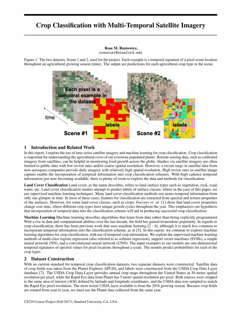
Figure 1: The two datasets, Scene 1 and 2, used for the project. Each example is a temporal signature of a pixel scene locationthroughout an agricultural growing season (time). The output are predictions for each agricultural crop type in the scene.

1 Introduction and Related WorkIn this report, I explore the use of time series satellite imagery and machine learning for crop classification. Crop classificationis important for understanding the agricultural cover of our evermore populated planet. Remote sensing data, such as calibratedimagery from satellites, can be helpful in monitoring food growth across the globe. Studies via satellite imagery are oftenlimited to public data with low revisit rates and/or coarse spatial resolution. However, a recent surge in satellite data fromnew-aerospace companies provide daily imagery with relatively high spatial resolution. High revisit rates in satellite imagecapture enable the incorporation of temporal information into crop classification schemes. With high cadence temporalinformation just now becoming available, there is plenty of room to explore the data and methods for classification.

Land Cover Classification Land cover, as the name describes, refers to land surface types such as vegetation, rock, road,water, etc. Land cover classification studies attempt to predict labels of surface classes, where in the case of this paper, weuse supervised machine learning techniques. Many land cover classification methods use mono-temporal information fromonly one glimpse in time. In most of these cases, features for classification are extracted from spectral and texture propertiesof the surfaces. However, for some land cover classes, such as crops, Foerster et. al. [1] show that land cover propertieschange over time, where different crop types have unique growth cycles throughout the year. This emphasizes our hypothesisthat incorporation of temporal data into the classification scheme will aid in producing successful crop classification.

Machine Learning Machine learning describes algorithms that learn from data rather than being explicitly programmed.With a rise in data and computational abilities over the last decade, the field has gained tremendous popularity. In regards tocrop classification, there has been previous work that uses machine learning [2 - 4], although it is much less common toincorporate temporal information into the classification scheme, as in [5]. In this report, we continue to explore machinelearning algorithms for crop classification, with use of temporal crop information. We explore the supervised machine learningmethods of multi-class logistic regression (also referred to as softmax regression), support vector machines (SVMs), a simpleneural network (NN), and a convolutional neural network (CNN). The input examples to our models are one-dimensionaltemporal signatures of spectral values for pixel locations throughout a scene. The models predict probabilities for each of thecrop types.

2 Dataset ConstructionWith no current standard for temporal crop classification datasets, two separate datasets were constructed. Satellite dataof crop fields was taken from the Planet Explorer API [6], and labels were constructed from the USDA Crop Data Layerdatabase [7]. The USDA Crop Data Layer provides annual crop maps throughout the United States at 30 meter spatialresolution per pixel, while the Rapid Eye data from Planet has 5 meter spatial resolution per pixel. Both sources were croppedto the same area of interest (AOI) defined by latitude and longitude coordinates, and the USDA data was sampled to matchthe Rapid Eye pixel resolution. The most recent USDA layer available is from the 2016 growing season. Because crop fieldsare rotated from year to year, we must use the Planet data collected from the same year.

CS229 Course Project (Fall 2017), Stanford University, CA, USA.

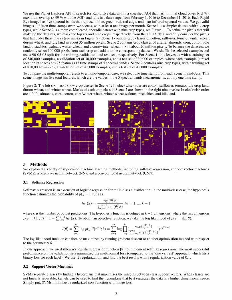
We use the Planet Explorer API to search for Rapid Eye data within a specified AOI that has minimal cloud cover (< 5 %),maximum overlap (> 99 % with the AOI), and falls in a date range from February 1, 2016 to December 31, 2016. Each RapidEye image has five spectral bands that represent blue, green, red, red edge, and near infrared spectral values. We get validimages at fifteen time stamps over two scenes, with at least one image per month. Scene 1 is a simpler dataset with six croptypes, while Scene 2 is a more complicated, sporadic dataset with nine crop types, see Figure 1. To define the pixels that willmake up the datasets, we mask the top six and nine crops, respectively, from the USDA data, and only consider the pixelsthat fall under these masks (see masks in Figure 2). Scene 1 contains crop classes of cotton, safflower, tomato, winter wheat,durum wheat, and idle land in about 35 million pixels. Scene 2 contains crop classes of alfalfa, almonds, corn, cotton, idleland, pistachios, walnuts, winter wheat, and a corn/winter wheat mix in about 20 million pixels. To balance the datasets, werandomly select 100,000 pixels from each crop and add it to the corresponding dataset. We shuffle the selected examples anduse a 90-05-05 split for the training, validation, and test sets, respectively. For Scene 1, this leaves us with a training setof 540,000 examples, a validation set of 30,000 examples, and a test set of 30,000 examples, where each example (a pixellocation in space) has 75 features (15 time stamps of 5 spectral bands). Scene 2 contains nine crop types, with a training setof 810,000 examples, a validation set of 45,000 examples, and a test set of 45,000 examples.

To compare the multi-temporal results to a mono-temporal case, we select one time stamp from each scene in mid-July. Thisscene image has five total features, which are the values in the 5 spectral bands measurements, at only one time stamp.

Figure 2: The left six masks show crop classes in Scene 1: In clockwise order are cotton, safflower, tomato, idle crop land,durum wheat, and winter wheat. Masks of each crop class in Scene 2 are shown in the right nine masks: In clockwise orderare alfalfa, almonds, corn, cotton, corn/winter wheat, winter wheat,walnuts, pistachios, and idle land.

3 MethodsWe explored a variety of supervised machine learning methods, including softmax regression, support vector machines(SVMs), a one-layer neural network (NN), and a convolutional neural network (CNN).

3.1 Softmax Regression

Softmax regression is an extension of logistic regression for multi-class classification. In the multi-class case, the hypothesisfunction estimates the probability of p(y = i|x; θ) as

hθi(x) =exp(θTi x)∑k−1j=1 exp(θTi x)

,∀i = 1, ..., k − 1

where k is the number of output predictions. The hypothesis function is defined in k−1 dimensions, where the last dimensionp(y = k|x; θ) = 1−

∑k−1i=1 hθi(x). To obtain an objective function, we take the log likelihood of p(y = i|x; θ):

l(θ) =

m∑i=1

log p(y(i)|x(i); θ) =

m∑i=1

log

k∏l=1

(exp(θTl x

1)∑kj=1 exp(θTj x

(i)))1y

(i)=l

The log-likelihood function can then be maximized by running gradient descent or another optimization method with respectto the parameters θ.

In our approach, we used sklearn’s logistic regression function [8] to implement softmax regression. The most successfulperformance on the validation sets minimized the multinomial loss (compared to the ’one vs. rest’ approach, which fits abinary loss for each label). We use l2 regularization, and find the best results with a regularization value of 0.1.

3.2 Support Vector Machines

SVMs separate classes by finding a hyperplane that maximizes the margins between class support vectors. When classes arenot linearly separable, kernels can be used to find the hyperplane that best separates the data in a higher dimensional space.Simply put, SVMs minimize a regularized cost function with hinge loss.

2

Hinge loss is defined as: L(z, y) = max(0, 1− yz). The goal of SVMs is to find w ∈ Rn and b ∈ R that minimize

J(w, b) = Σmi=1L(wx(i) − b, y(i)) +λ

2||w||2

We use sklearn’s SVM functions [9] to implement the SVM classifier. The most successful performance on the validationsets used a RBF kernel with a small regularization value, λ = 1e-6, and a gamma value of 0.1, which is used in the sklearnimplementation to specify the importance of each individual example. As gamma was increased, the training score increased,while validation score decreased. This indicates that a large value of gamma leads to over fitting. As regularization weightdecreased, validation score increased. In this case, increasing the regularization weight does not seem to help the model,but rather hurt it. The SVM models were trained on a smaller training set of 60,000 examples to produce these results. Thevalidation and test sets remained the same.

3.3 Simple Neural Network (NN)

At a high level, NNs mimic neural connections inspired by the human brain. As long as the path of each mathematicalconnection is differentiable, the weights of the network can be learned through backpropagation. We implement a simpleone-layer neural network with the Keras sequential modeling framework [10]. The model has a hidden layer with 200neurons, uses a rectified linear unit (relu) activation function for the hidden layer and a softmax activation function at theoutput, cross entropy loss, a dropout rate of 0.1, and a regularization strength of λ = 1e-5. Adadelta [11], a technique thatuses an adaptive learning rate, is used to optimize for the model parameters. The Xavier initialization method [12] is used toinitialize weights, and biases are initialized to zero. We train for 100 epochs with a batch size of 1000 examples. The samenumber of hidden units and output predictions are used in the mono-temporal case, except that the model input only has fivefeatures, and so the model is also retrained for this case.

3.4 Convolutional Neural Network (CNN)

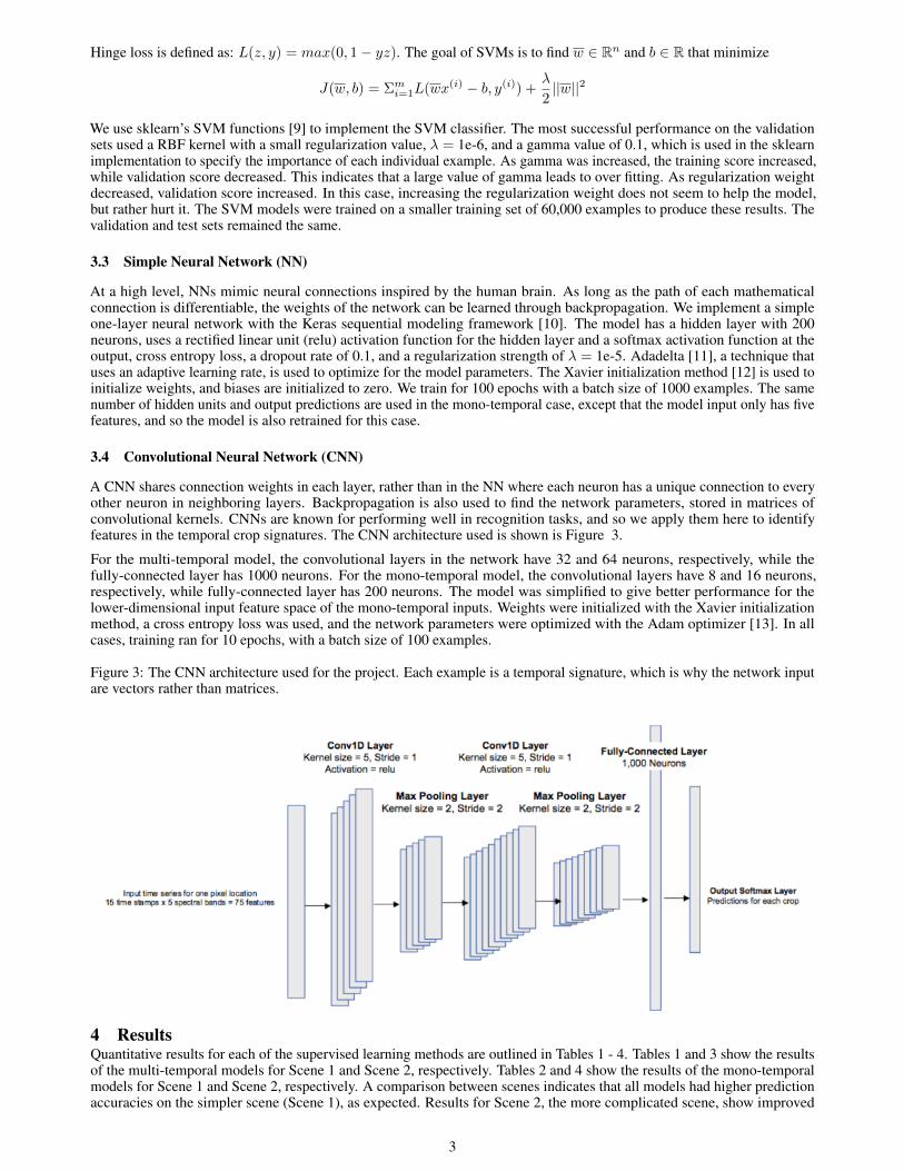
A CNN shares connection weights in each layer, rather than in the NN where each neuron has a unique connection to everyother neuron in neighboring layers. Backpropagation is also used to find the network parameters, stored in matrices ofconvolutional kernels. CNNs are known for performing well in recognition tasks, and so we apply them here to identifyfeatures in the temporal crop signatures. The CNN architecture used is shown is Figure 3.

For the multi-temporal model, the convolutional layers in the network have 32 and 64 neurons, respectively, while thefully-connected layer has 1000 neurons. For the mono-temporal model, the convolutional layers have 8 and 16 neurons,respectively, while fully-connected layer has 200 neurons. The model was simplified to give better performance for thelower-dimensional input feature space of the mono-temporal inputs. Weights were initialized with the Xavier initializationmethod, a cross entropy loss was used, and the network parameters were optimized with the Adam optimizer [13]. In allcases, training ran for 10 epochs, with a batch size of 100 examples.

Figure 3: The CNN architecture used for the project. Each example is a temporal signature, which is why the network inputare vectors rather than matrices.

4 ResultsQuantitative results for each of the supervised learning methods are outlined in Tables 1 - 4. Tables 1 and 3 show the resultsof the multi-temporal models for Scene 1 and Scene 2, respectively. Tables 2 and 4 show the results of the mono-temporalmodels for Scene 1 and Scene 2, respectively. A comparison between scenes indicates that all models had higher predictionaccuracies on the simpler scene (Scene 1), as expected. Results for Scene 2, the more complicated scene, show improved

3

prediction accuracy as the models become more complicated, going from left to right in table columns. A comparisonbetween multi-temporal and mono-temporal results shows an increase in performance from added temporal information.This provides an important insight that temporal information is helpful for crop classification, showing that crops havedistinguishable temporal signatures throughout the growing season.

Table 1: Scene 1 Multi-Temporal ResultsSoftmax Reg. SVMs Simple NN CNN

Train Accuracy 92.38 96.46 92.88 95.66Test Accuracy 92.06 92.21 92.06 92.64

Table 2: Scene 1 Mono-Temporal ResultsSoftmax Reg. SVMs Simple NN CNN


Table 3: Scene 2 Multi-Temporal ResultsSoftmax Reg. SVMs Simple NN CNN


Table 4: Scene 2 Mono-Temporal ResultsSoftmax Reg. SVMs Simple NN CNN


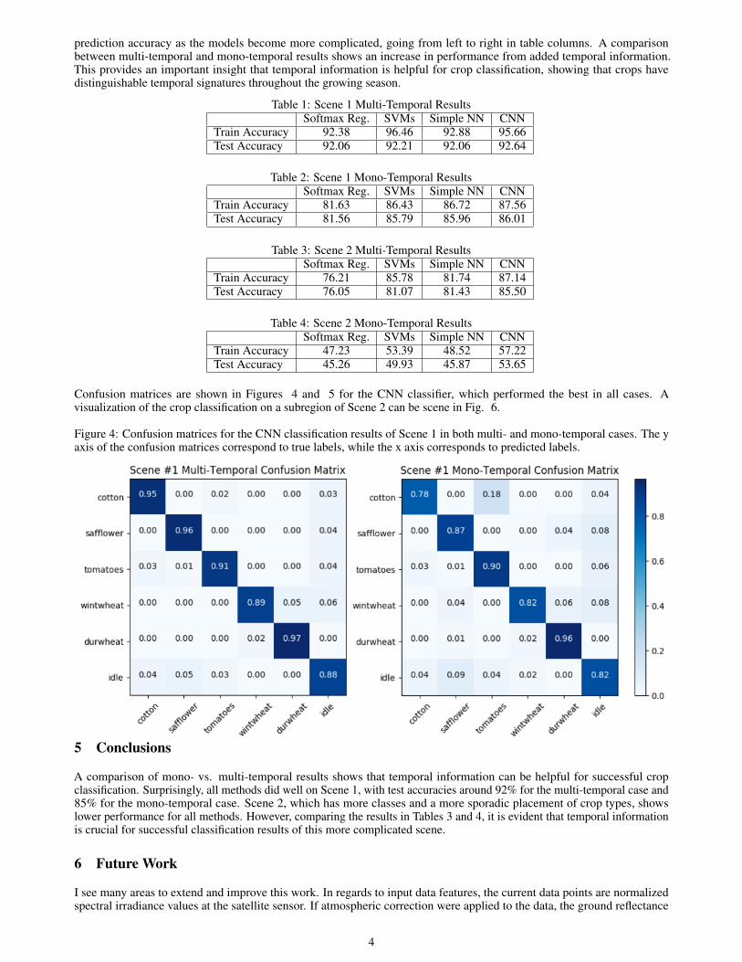
Confusion matrices are shown in Figures 4 and 5 for the CNN classifier, which performed the best in all cases. Avisualization of the crop classification on a subregion of Scene 2 can be scene in Fig. 6.

Figure 4: Confusion matrices for the CNN classification results of Scene 1 in both multi- and mono-temporal cases. The yaxis of the confusion matrices correspond to true labels, while the x axis corresponds to predicted labels.

5 Conclusions

A comparison of mono- vs. multi-temporal results shows that temporal information can be helpful for successful cropclassification. Surprisingly, all methods did well on Scene 1, with test accuracies around 92% for the multi-temporal case and85% for the mono-temporal case. Scene 2, which has more classes and a more sporadic placement of crop types, showslower performance for all methods. However, comparing the results in Tables 3 and 4, it is evident that temporal informationis crucial for successful classification results of this more complicated scene.

6 Future Work

I see many areas to extend and improve this work. In regards to input data features, the current data points are normalizedspectral irradiance values at the satellite sensor. If atmospheric correction were applied to the data, the ground reflectance

4

Figure 5: Confusion matrices for the CNN classification results of Scene 2 in both multi- and mono-temporal cases. The yaxis of the confusion matrices correspond to true labels, while the x axis corresponds to predicted labels.

Figure 6: A qualitative visual result of the crop classification in an arbitrary region selected from Scene 2. The left imageshows the ground truth labels of the crops from the USDA database, while the right image shows the predicted labels fromthe CNN model. The resolution is clearly finer in the predicted labels, which is expected since the Rapid Eye data has 5mresolution (compared to the 30m resolution of the ground truth).

values would be invariant to illumination changes. This would yield more stable and consistent input features for training,which would also allow the model to generalize to other regions, regardless of illumination fluctuations. Textural features(such as from local binary patterns (LBP) or the gray level co-occurence matrix) may provide helpful spatial informationfrom pixels in local neighborhoods. Incorporation of spatial information will likely boost performance.

I would like to continue this work using Planet data from 2017 for a similar analysis once the USDA Crop Data Layer isreleased for the year. The current cadence of Planet satellites is near daily, providing even richer temporal informationcompared to what was used in this project with 2016 data (approximately one image per month). It would be interesting toinvestigate the performance of LSTMs on the temporal dataset, as well as semantic segmentation methods that take the entireimage as input.

5

7 Acknowledgments

I would like to thank Professor Andrew Ng and Professor Dan Boneh for a fantastic class in machine learning. I would alsolike to thank Kat Scott and the Image Analytics team at Planet Labs, who have provided guidance throughout this project andhave introduced me to Planet’s amazing set of global imagery.

8 Contributions

The project was completed by one student. Therefore, all contributions of work for this project has been completed by theauthor.

References

[1] Foerster, S. & Kaden, K. & Forster, M. & Itzerott, S. (2012) Crop type mapping using spectral-temporal profiles and phenologicalinformation, Computers and Electronics in Agriculture, 89, pp. 30–40.

[2] Peña, J., Gutierrez, P., Hervas-Martinez, C., Six, J., Plant, R., & Lopez-Granados, F. (2014) Object-Based Image Classification ofSummer Crops with Machine Learning Methods Remote Sensing, 6; doi:10.3390/rs6065019, pp. 5019–5041.

[3] Tripathi, M., & Maktedar, D. (2016). Recent machine learning based approaches for disease detection and classifica-tion of agricultural products IEEE International Conference on Computing Communication Control and Automation (ICCUBEA);doi:10.1109/ICCUBEA.2016.7860043

[4] Mishra, S., Mishra, D., & Harri, S. (2016). Applications of Machine Learning Techniques in Agricultural Crop Production: A ReviewPaper. Indian Journal of Science and Technology, 9; doi:10.17485/ijst/2016/v9i38/95032

[5] Rubwurm, M. & Korner, M. (2017) Multi-temporal land cover classification with long short-term memory neural networks TheInternational Archives of Photogrammetry, Remote Sensing, and Spatial Information Sciences (ISPRS), XLII-1/W1, pp. 551–558.

[6] Planet Explorer Beta, Planet Labs, https://www.planet.com/explorer/

[7] CropScape - Crop Data Layer, United States Department of Agriculture, National Agriculture Statistics Service,https://nassgeodata.gmu.edu/CropScape/

[8] Scikit learn, sklearn.linear_model.LogisticRegression, http://scikit-learn.org/stable/modules/generated/sklearn.linear_model.LogisticRegression.html

[9] Scikit learn, Support Vector Machines, http://scikit-learn.org/stable/modules/svm.html

[10] Keras, Getting started with the Keras Sequential model, Keras Documentation, https://keras.io/getting-started/sequential-model-guide/

[11] Glorot, X., & Bengio, Y. (2010). Understanding the difficulty of training deep feedforward neural networks, Proceedings of theThirteenth International Conference on Artificial Intelligence and Statistics, PLMR, 9: pp. 249–256.

[12] Zeiler, M. (2012). ADADELTA: An Adaptive Learning Rate Method, arXiv:1212.5701

[13] Kingma, D. P., & Ba, J. (2015). Adam: A method for Stochastic Optimization, 3rd International Conference for LearningRepresentations, San Diego

6

crop classiﬁcation with multi-temporal satellite...

Documents