Optical Microlithography XVII, Bruce W. Smith – Editor, Proceedings of SPIE Vol. 5377-207 (2004)

Critical evaluation of focus analysis methods

Bill Robertsa, Matthew McQuillana,b, Nicholas Loukaa, Terrence Zavecz#c , Patrick Reynoldsd, Mircea Dusae

a)Infineon Technologies, 6000 Technology Boulevard, Richmond VA 23150 b)Rochester Institute of Technology, Rochester, NY c)TEA Systems Corp., 65 Schlossburg St., Alburtis, PA 18011 d) Benchmark Technologies, 7-E Kimball Lane, Lynnfield, MA 01940 e)ASML, Suite 400, TS-TDC, 4800 Great America Parkway, Santa Clara, CA 95054

1. ABSTRACT Device Design criteria and product complexity have reduced the Focus Budget on today's technologies to near zero. Recent years have seen the introduction of a number of focus monitor methods involving new designs and processes that attempt more accurately or more easily to define the focus performance of our imaging systems.

We have evaluated several focus monitoring techniques and compared their relative strengths and speed. The objective of this study is to demonstrate each technology’s ability to evaluate exposure tool lens performance and quantify those factors that directly degrade depth-of-focus in the process. Baseline focus for process exposure and lens aerial image aberration analysis is evaluated using focus matrices. The remaining contributors to depth-of-focus (DOF) degradation are derived from the opto-mechanical interactions of the tool during full-wafer exposures. Full-wafer exposures, biased to –100 nm focus, were used in the determination of these error sources.

Exposing all test sequences on the same 193 nm scanner provided consistency of the comparison. A valid analytical comparison of the technologies was further guaranteed by using a single software tool, Weir PSFM software from Benchmark Technologies, to calibrate, analyze and model all metrology.

Two of the four techniques we evaluated were found to require focus matrices for analysis. This prohibited them from being able to analyze the fixed-focus exposure detractors to the DOF. One technique was found to be ineffective at the 193 nm because of the high-contrast response of the photoresists used.

An analysis of the aerial image was validated by comparison of each technique to the Z5 Zernike as measured by ASML’s ARTEMIS™ analysis. The ASML FOCAL™ and Benchmark PGM targets, both replicating dense- packed feature response, best tracked ARTEMIS signature.

A whole-wafer, fixed exposure tool focus analysis is used to evaluate wafer, photoresist and dynamic scan contributions to the focus budget. Of the four techniques considered only the PSFM and PGM patterns could be used for this evaluation. Performance response is reported for detractors involving the wafer as well as the mechanical scan direction of the reticle stage.

Keywords: Lithography, exposure tool, aberrations, focus, models, Zernike, Line-end shortening, LES, lens, aberrations, IDOF., Depth-of-Focus, Resolution, scan-slit, astigmatism, scanner

# For additional correspondence address questions to tzavecz@enter.net. ((01) 610 682 - 4146

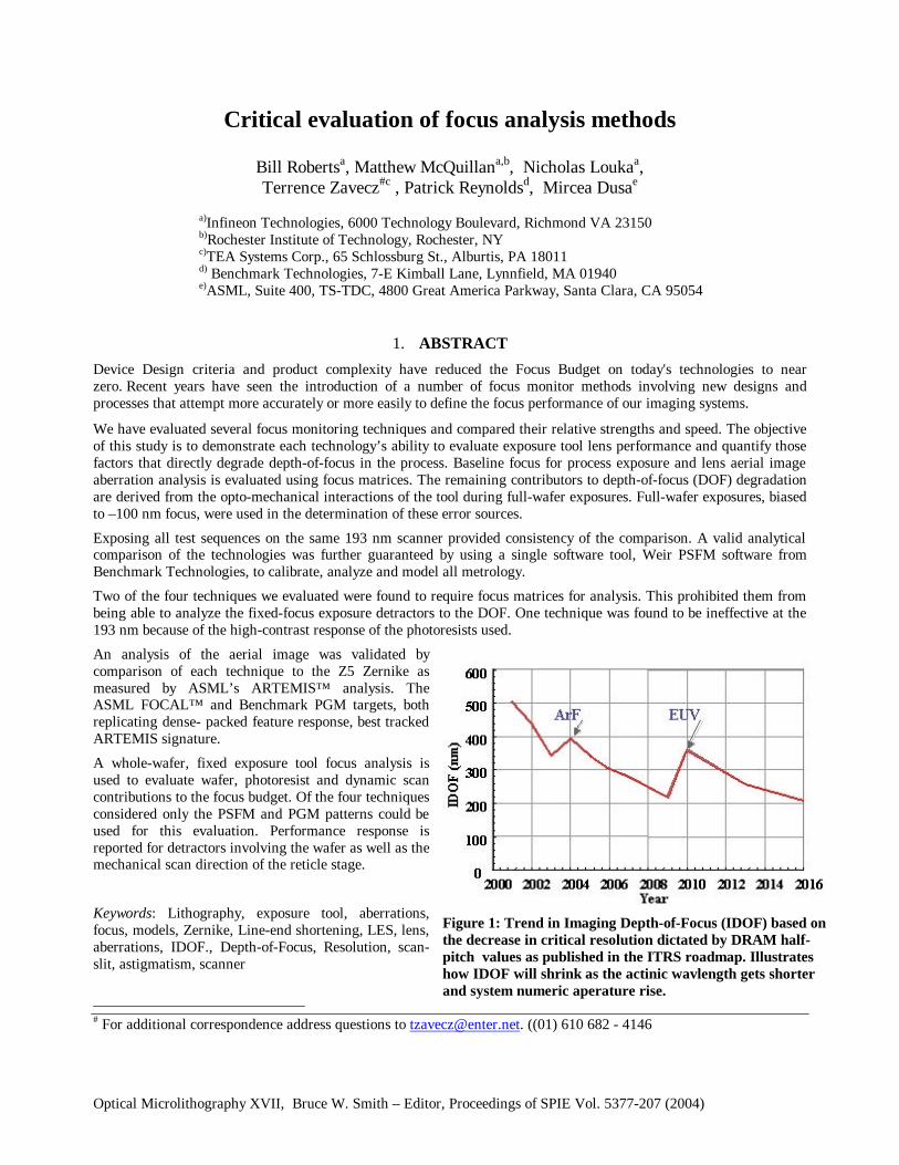
Figure 1: Trend in Imaging Depth-of-Focus (IDOF) based on the decrease in critical resolution dictated by DRAM half-pitch values as published in the ITRS roadmap. Illustrates how IDOF will shrink as the actinic wavlength gets shorter and system numeric aperature rise.

Proc. SPIE Vol. 5377 – 207 - Page 2 -

2. INTRODUCTION

Focus and dose have always been the primary variables of concern in the lithographic process. The influence of Dose is easily measured using the linear behavior of critical feature sizes. Focus is by far the most difficult to manage because of the indirect methods that must be employed in its metrology. Our understanding of the variable is challenged by the broad variability incurred during imaging through perturbations introduced by optical, mechanical and substrate sources in the process.

Difficulties in obtaining focus metrology are compounded by the fact that the tolerable depth of focus for successful imaging of the patterns is continually being driven down by our industry’s ongoing quest for smaller feature sizes and greater packing density. The depth-of-focus variable, being directly derived as a corollary to the Raleigh criteria of resolution as proportional to the actinic wavelength of the system and inversely to the square of the numeric aperture, is thereby also reduced in our quest for smaller features.

The ITRS Roadmap can be used as a source for projecting the imaging depth-of-focus (IDOF) by assuming the critical feature size will follow the DRAM half-pitch and that ArF, F2 and EUV Lithography are introduced respectively in 2004, 2007 and 2010. On this basis, Figure 1 predicts a systematic reduction in the IDOF contributing to a corresponding reduction in process margins.1, 2

The IDOF is further degraded beyond the theoretical value by aberrations as well as manufacturing-induced perturbations in the optical train and electro-mechanical–optical interaction during scanning of the slit.

Historically, lithographic focus has been determined manually by microscopic examination of threshold-resolution line/space patterns as exposed in a focus matrix (FM). More advanced methods employed the microscopic observation of dot arrays through focus or the shortening of tapered features or “daggers”.3

More automated empirical techniques have employed FM arrays of critical-sized features measured using optical or Scanning Electron Microscopic (SEM) tools to generate a family of curves representing linewidth change through focus, which is called a Bossung plot.4 From these plots, the best focus and depth of focus can be estimated based on the design-tolerable limits of feature size. More recently this concept has been employed using the characteristic shortening of line-ends (LES) to emulate feature pattern shifts with defocus.5

These methods all suffer from a quadratic response of the measured variable with focus. This symmetric response curve limits the functionality of the technique for process automation because the technique cannot discriminate between focus errors that lie above or below the point of best focus. The automation problem had been inadvertently solved by Brunner in 1993 by the introduction of a new concept focus metrology tool that employed a ninety (90) degree phase shift element that resulted in an apparent shifting of the feature’s position in the field. The key solution here is that the shift was now linearly related to the focus error. This product is called the phase-shift focus monitor.6 Phase Shift Focus Monitor (PSFM) - Focus features could now be directly measured using a positional feature metrology overlay tool.

The phase shift concept best replicated the focus response of isolated lines because of the large features sizes used in the design. A dense-packed feature’s response to focus is quite different and even more critical than those of isolated lines. To address the response of dense structures ASML uses their alignment techniques to measure the Fourier transform response of gratings in an automated analysis procedure called FOCAL.7 FOCAL response works well for focus-matrices but exhibits a symmetric, quadratic response to defocus similar to LES and the other non-PSFM methods.

The use of blaze-gratings provides another method of dense-structure focus-response evaluation and Zernike extraction.8 These structures form a two-beam interferometer that, by changing the angular orientation of the grating, allows the intensity profile of the exit pupil to be mapped and correlated to the aberrations of the lens. Blaze gratings are addressed in another paper at this conference.9

More recently the PSFM concept was extrapolated from phase offsets of isolated features to an implementation on line/space gratings10, 11. These new structures, referred to as Phase Grating Focus Monitors (PGM), now replicate a shift in the pattern that is linear and asymmetric with focus for dense structures. This behavior lends itself well to optimal focus mapping across the lens for focus matrices and quite uniquely to analyses where the exposure tool focus is fixed for evaluation of focus response across the entire wafer and under all conditions of stage travel and exposure. The PSFM and PGM toolset used in unison for an analysis therefore provide a complete package for evaluation of focus response for both isolated and dense-packed structures.

Proc. SPIE Vol. 5377 – 207 - Page 3 -

2.1. Objectives

Four methods of focus metrology have been comparatively evaluated in their capability to be used as both a lens focus-diagnostic toolset and as a daily focus monitor of depth of focus:

?? Line End Shortening (LES) ?? ASML FOCAL™ ?? PSFM Phase shift focus monitor patterns for isolated structures and ?? PGM Phase-grating focus monitor patterns for dense-packed feature sets.

To obtain a thorough understanding of an exposure tool’s depth-of-focus response the user needs to measure those detractors contributed by the lens and from the electro-mechanical elements of the scanned exposure. This involves an analysis of:

?? The average or “Best Focus” of the tool o For use in baseline process setup during exposure adjustment.

?? A mapping of the lens aerial image planarity o To assist in an understanding of the base lens and scan aberrations and

?? A characterization of the across-wafer behavior of focus where fields are exposed at constant tool focus covering the wafer

o Thus providing a quantification of the opto-mechanical depth-of-focus detractors of wafer planarity, edge bead, auto-leveling and slit-scan contributions to the focus error budget.

3. PRINCIPALS OF THE COMPARISON

For consistency, exposures were made on a single ASML PAS \1100B slit-scanner. However the behavior reported here is not tool or model specific. Responses similar to and even exceeding these have been observed on other exposure tools both from this and other vendors in the market. The exposure source is ArF. PSFM 180, PSFM 160, PGM and LES metrology data were gathered using a Nikon NRM overlay tool. The PSFM designations indicate the metrology response for 180 and 160 nm isolated structure targets directly. The ASML scanner was also used in a self-analysis of the FOCAL data as presented. Aerial image analysis of the lens contribution is performed using focus matrices at the exposure setups detailed in table #1. The fixed-focus analysis of opto-mechanical and process perturbations uses the same dose as shown but biased in tool focus offset to –100 nanometers (nm). Analysis objective and the methods used for each are shown in table #2.

All of the techniques could be used with focus matrices as a focus monitor and in an analysis of the exposure tool’s Best Focus estimation of the lens focus aberrations. However, only the PSFM and PGM technologies allow the analysis of fixed-focus perturbations resulting from wafer film and slit-scan direction contributions.

PGM and FOCAL employed features that correspond in size and packing design. However, we could not perform an immediate and direct comparison between the two techniques because the FOCAL-analysis required an extended exposure tool exposure and metrology time of over four hours for an analysis. We therefore used the most recent FOCAL analysis available, which unfortunately incorporated a ring-aperture exposure setting as opposed to the standard exposure of the other data sets.

Each focus-metrology method employs its own proprietary models and analysis methods that

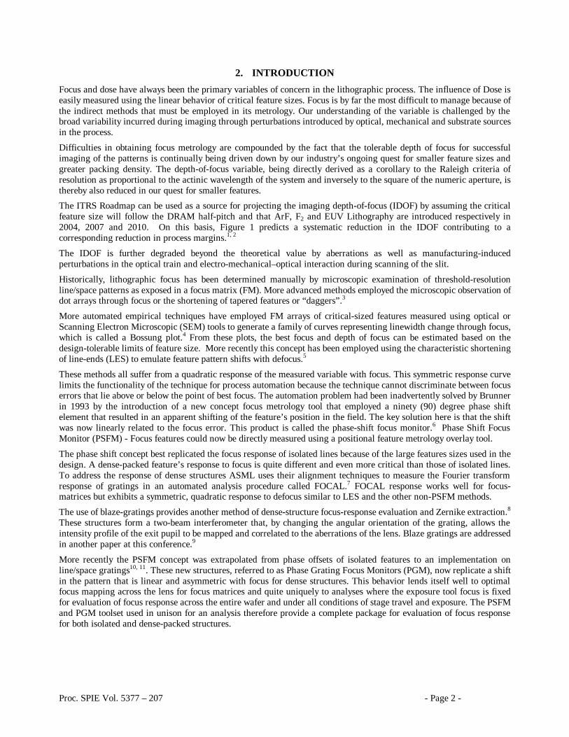
Method Dose (mj) Focus NA Sigma Cycle Time

LES 17 FM 1.5 hr

FOCAL 360 FM 0.75 0.55/0.85 Ring 4.5 hours

PSFM 17 FM 0.7 0.349 1.5 hr

PGM 22.5 FM 0.7 0.349 1.5 hr

Table 1: Summary of exposure conditions for each of the four analysis methods.

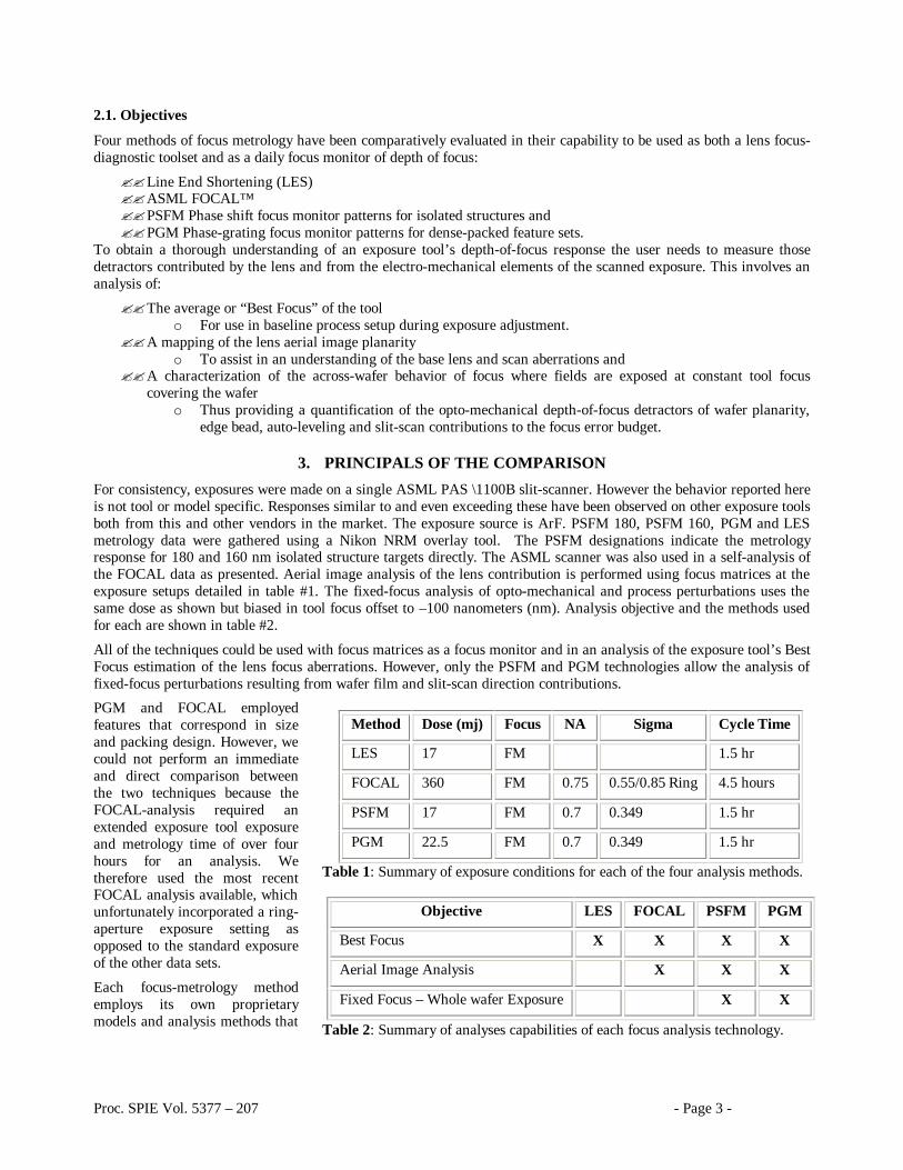
Objective LES FOCAL PSFM PGM

Best Focus X X X X

Aerial Image Analysis X X X

Fixed Focus – Whole wafer Exposure X X

Table 2: Summary of analyses capabilities of each focus analysis technology.

Proc. SPIE Vol. 5377 – 207 - Page 4 -

make a direct performance comparison difficult or impossible. This study employed the Weir PSFM software from Benchmark Technologies to gather the data, analyze and model results in a consistent framework thereby avoiding analysis inconsistencies.

3.1 Validation of the techniques

The functionality of LES, Focal, PSFM and the PGM techniques were confirmed wherever possible by correlating results with characterizations of the system using other methods. Data was obtained from the same exposure tool using the ASML ARTEMIS® method of Zernike coefficient extrapolation to correlate the lens-focus measured Astigmatism with the ARTEMIS measured Z5 coefficient.12 Only the Zernike Z5 coefficient was used for the comparison and was felt to be adequate since the original study was performed under a dynamic scan condition. Under these conditions, the Zernike evaluation method of ARTEMIS also calculates “Lithographer’s” Astigmatism as the (Y-X) focus difference at each site12. The net effect of the dynamic exposure-scan is to average out the Y-scan oriented aberrations so across-slit Zernike values actually only represent perturbations as measured in the lens-slit direction.

The method of the fixed focus, whole wafer study is to evaluate focus variation across the wafer, at it’s edges and across each individual field while the optimum tool focus value is fixed. That is, the technique emulates the behavior of the exposure tool during daily lot exposure. In this phase the exposure tool itself was used as the standard for validation by programming some field-exposures with known exposure tool focus offsets. Selected fields were offset in focus by amounts as small as 70 nm. Valid operation of the focus-method was confirmed by the technique’s level of resolution of these offsets.

4. BEST FOCUS ANALYSIS

4.1. Best Focus

Optimum focus for any feature set depends upon the feature size and duty cycle. Most techniques respond quadratically to defocus. As a result, a derivation of the optimum focus for process exposure typically involves a focus matrix. Modeling across the focus matrix also reduces the influence of local process variation.

Line End Shortening (LES) does not work efficiently for 193 nm and lower wavelengths. For longer wavelengths, best focus can be quickly analyzed using the LES technique by measuring the effective line length as a function of focus. However, the high-contrast photoresists used at the 193 nm wavelength lowers the accuracy of the technique beyond acceptable limits.

FOCAL, PSFM 180, PSFM 160 and the PGM patterns all were able to easily accommodate the 193 nm exposure sequence. Comparative results are presented to the next section.

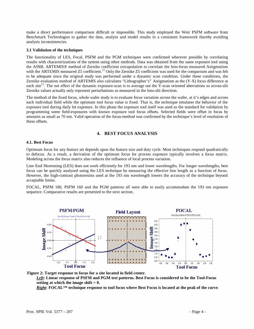
Figure 2: Target response to focus for a site located in field center.

Left: Linear response of PSFM and PGM test patterns. Best Focus is considered to be the Tool-Focus setting at which the image shift = 0. Right: FOCAL™ technique response to tool focus where Best Focus is located at the peak of the curve.

Proc. SPIE Vol. 5377 – 207 - Page 5 -

4.2. Aerial image analysis

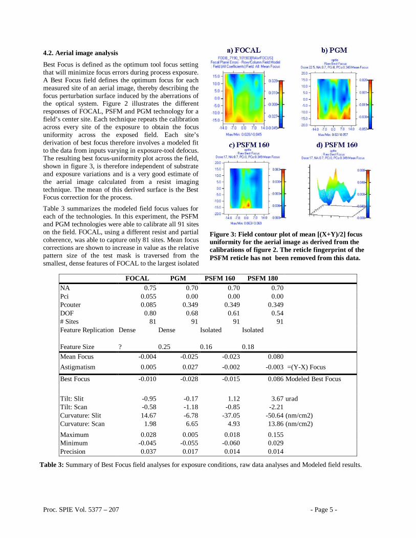
Best Focus is defined as the optimum tool focus setting that will minimize focus errors during process exposure. A Best Focus field defines the optimum focus for each measured site of an aerial image, thereby describing the focus perturbation surface induced by the aberrations of the optical system. Figure 2 illustrates the different responses of FOCAL, PSFM and PGM technology for a field’s center site. Each technique repeats the calibration across every site of the exposure to obtain the focus uniformity across the exposed field. Each site’s derivation of best focus therefore involves a modeled fit to the data from inputs varying in exposure-tool defocus. The resulting best focus-uniformity plot across the field, shown in figure 3, is therefore independent of substrate and exposure variations and is a very good estimate of the aerial image calculated from a resist imaging technique. The mean of this derived surface is the Best Focus correction for the process.

Table 3 summarizes the modeled field focus values for each of the technologies. In this experiment, the PSFM and PGM technologies were able to calibrate all 91 sites on the field. FOCAL, using a different resist and partial coherence, was able to capture only 81 sites. Mean focus corrections are shown to increase in value as the relative pattern size of the test mask is traversed from the smallest, dense features of FOCAL to the largest isolated

Figure 3: Field contour plot of mean [(X+Y)/2] focus uniformity for the aerial image as derived from the calibrations of figure 2. The reticle fingerprint of the PSFM reticle has not been removed from this data.

FOCAL PGM PSFM 160 PSFM 180 NA 0.75 0.70 0.70 0.70 Pci 0.055 0.00 0.00 0.00 Pcouter 0.085 0.349 0.349 0.349 DOF 0.80 0.68 0.61 0.54 # Sites 81 91 91 91 Feature Replication Dense Dense Isolated Isolated

Feature Size ? 0.25 0.16 0.18 Mean Focus -0.004 -0.025 -0.023 0.080 Astigmatism 0.005 0.027 -0.002 -0.003 =(Y-X) Focus

Best Focus -0.010 -0.028 -0.015 0.086 Modeled Best Focus Tilt: Slit -0.95 -0.17 1.12 3.67 urad Tilt: Scan -0.58 -1.18 -0.85 -2.21 Curvature: Slit 14.67 -6.78 -37.05 -50.64 (nm/cm2) Curvature: Scan 1.98 6.65 4.93 13.86 (nm/cm2)

Maximum 0.028 0.005 0.018 0.155 Minimum -0.045 -0.055 -0.060 0.029 Precision 0.037 0.017 0.014 0.014

Table 3: Summary of Best Focus field analyses for exposure conditions, raw data analyses and Modeled field results.

Proc. SPIE Vol. 5377 – 207 - Page 6 -

patterns of the PSFM 180 target.

The PSFM 180 target exhibits an anomalous shift in best focus from that of the other PSFM 160, PGM and FOCAL results. This shift may be the result of patterning errors on the PSFM target selected. Simulations have shown that the PSFM aerial image shift is weakly sensitive to changes in the size of the chrome reticle pattern if one side of the box pattern is significantly different in width from it’s opposite edge. A significant offset in feature size will therefore result in a fixed offset of the calculated best focus and could explain the shift seen with the PSFM 180 target. The experiment did not evaluate the data for the presence or absence of signatures that may result from reticle patterning errors. This artifact is an offset and will not influence the computation of focus variations as encountered when examining focus uniformity across a wafer. PGM targets, because of their small chrome-feature design, are not sensitive to this shift.

If present, etch depth variations during reticle manufacture influence the slope of the calibration. However the presence of any slope variations are removed from the computation since each site is separately calibrated.

Weir PSFM used a 2nd order expansion model, equation 1, to evaluate coefficients corresponding to piston (focus offset=A), field tilt (=B) and curvature (=C) for each focus metrology method.

Focus = A + Bx + Cx2 … .. [1]

The slit-and-scan nature of scan exposure encourages each of the coefficients to be separately calculated for X and Y Cartesian coordinates. Exposure tool process corrections however are reported for the average of the two axes best focus values = (Xfocus + Yfocus)/2.

X-focus values record the response to defocus of vertical-oriented feature edges and also represent the contribution of the lens-slit to the IDOF. Horizontal feature edge response is reported by Y-scan values. The Y-scan axis is subjected to the scan averaging of the reticle-scan stage.

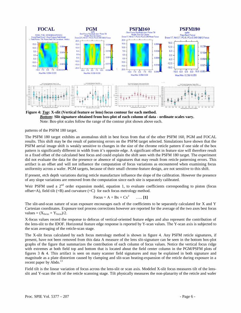
The X-slit focus calculated by each focus metrology method is shown in figure 4. Any PSFM reticle signatures, if present, have not been removed from this data A measure of the lens slit-signature can be seen in the bottom box-plot graphs of the figure that summarizes the contribution of each column of focus values. Notice the vertical focus ridge with extremes at both field top and bottom that is located about the field center column in the PGM/PSFM plots of figures 3 & 4. This artifact is seen on many scanner field signatures and may be explained in both signature and magnitude as a plate distortion caused by clamping and slit-scan heating-expansion of the reticle during exposure in a recent paper by Abdo.13

Field tilt is the linear variation of focus across the lens-slit or scan axis. Modeled X-slit focus measures tilt of the lens-slit and Y-scan the tilt of the reticle scanning stage. Tilt physically measures the non-planarity of the reticle and wafer

Figure 4: Top: X-slit (Vertical feature or lens) focus contour for each method.

Bottom: Slit signature obtained from box-plot of each column of data - ordinate scales vary. Note: Box-plot scales follow the range of the contour plot shown above each.

Proc. SPIE Vol. 5377 – 207 - Page 7 -

planes. The focus-matrix method of exposure records the average aerial image value of the scanner. The scanner however exposes bi-directionally, scanning the reticle up or down over the exposure slit. As a result, differences in field tilt result from hysteresis of the physical travel of the scan and accelerations typically found at the start and termination of the exposure.

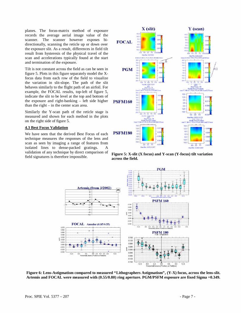
Tilt is not constant across the field as can be seen in figure 5. Plots in this figure separately model the X-focus data from each row of the field to visualize the variation in slit-slope. The path of the slit behaves similarly to the flight path of an airfoil. For example, the FOCAL results, top-left of figure 5, indicate the slit to be level at the top and bottom of the exposure and right-banking – left side higher than the right – in the center scan area.

Similarly the Y-scan path of the reticle stage is measured and shown for each method in the plots on the right side of figure 5.

4.3 Best Focus Validation

We have seen that the derived Best Focus of each technique measures the responses of the lens and scan as seen by imaging a range of features from isolated lines to dense-packed gratings. A validation of any technique by direct comparison of field signatures is therefore impossible.

Figure 5: X-slit (X focus) and Y-scan (Y-focus) tilt variation across the field.

Figure 6: Lens-Astigmatism compared to measured “Lithographers Astigmatism”, (Y-X) focus, across the lens-slit. Artemis and FOCAL were measured with (0.55/0.80) ring aperture. PGM/PSFM exposure are fixed Sigma =0.349.

Proc. SPIE Vol. 5377 – 207 - Page 8 -

The lens for this scanner was previously evaluated using the ARTEMIS technique of ASML, plotting the Z5 coefficient in the upper-left plot of figure 6.

The remaining graphs of figure 6 plot the (Y-X) focus values calculated for each best focus field as a function of their location in the slit. This is sometimes known as “Lithographers Astigmatism” and is a more useful evaluation for the process engineer since the majority of pattern features are Cartesian oriented by design.

Note that the displayed astigmatic contribution of the ARTEMIS Z5 coefficient’s magnitude is exceeded by all other methods. However, both the FOCAL and PGM techniques faithfully replicate the signature, particularly in the center of the lens. Variation at lens edges can be explained by variations in response of the exit pupil to the image frequencies employed by each method’s pattern and the fact that the FOCAL and ARTEMIS analyses used ring apertures.

5. WHOLE-WAFER FOCUS

5.1 Fixed-Focus metrology validation

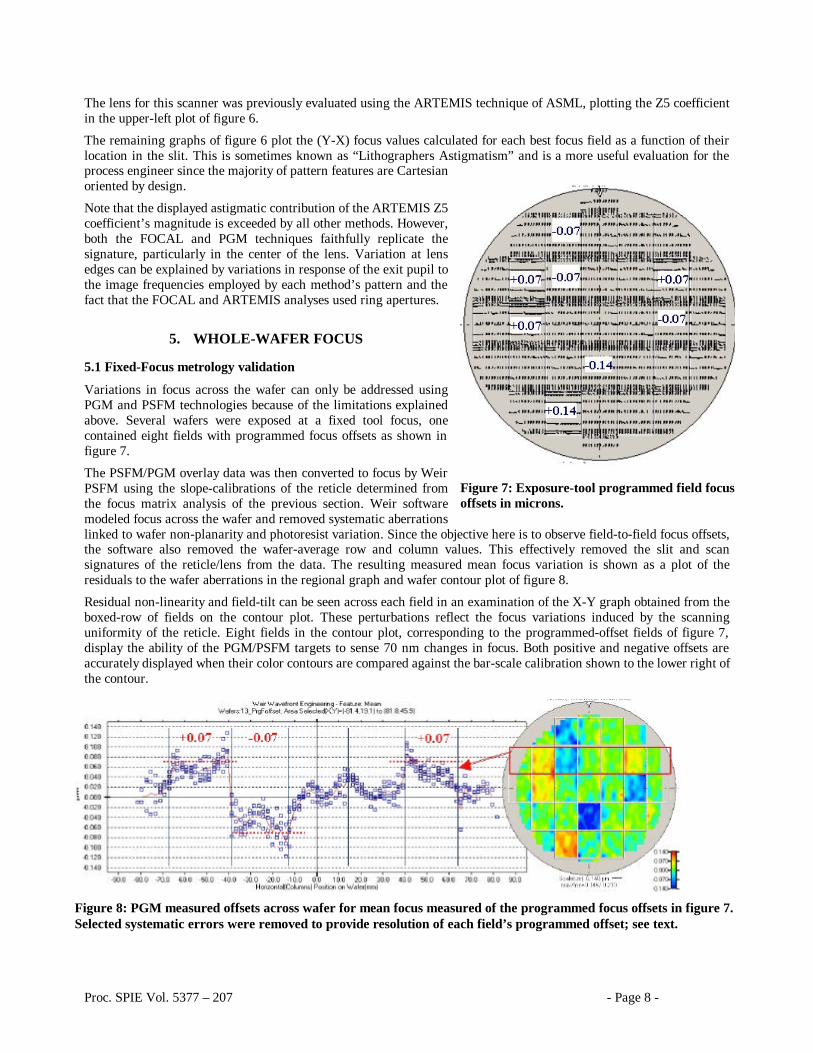
Variations in focus across the wafer can only be addressed using PGM and PSFM technologies because of the limitations explained above. Several wafers were exposed at a fixed tool focus, one contained eight fields with programmed focus offsets as shown in figure 7.

The PSFM/PGM overlay data was then converted to focus by Weir PSFM using the slope-calibrations of the reticle determined from the focus matrix analysis of the previous section. Weir software modeled focus across the wafer and removed systematic aberrations linked to wafer non-planarity and photoresist variation. Since the objective here is to observe field-to-field focus offsets, the software also removed the wafer-average row and column values. This effectively removed the slit and scan signatures of the reticle/lens from the data. The resulting measured mean focus variation is shown as a plot of the residuals to the wafer aberrations in the regional graph and wafer contour plot of figure 8.

Residual non-linearity and field-tilt can be seen across each field in an examination of the X-Y graph obtained from the boxed-row of fields on the contour plot. These perturbations reflect the focus variations induced by the scanning uniformity of the reticle. Eight fields in the contour plot, corresponding to the programmed-offset fields of figure 7, display the ability of the PGM/PSFM targets to sense 70 nm changes in focus. Both positive and negative offsets are accurately displayed when their color contours are compared against the bar-scale calibration shown to the lower right of the contour.

Figure 7: Exposure-tool programmed field focus offsets in microns.

Figure 8: PGM measured offsets across wafer for mean focus measured of the programmed focus offsets in figure 7. Selected systematic errors were removed to provide resolution of each field’s programmed offset; see text.

Proc. SPIE Vol. 5377 – 207 - Page 9 -

A more exacting analysis of the focus can be seen in the graph on the left side of figure 8. Using the mouse to drag a box around the dice as shown in the red box on the wafer contour generated this graph. Focus variations in this area are plotted as a function of their X location across the wafer. The plot clearly shows the 70 nm step induced by the programmed offset. We can also see an induced tilt of the field in the second die from the right side of the wafer. The tendency for a tool to induce tilt because of programmed focus offset or a wafer’s edge suggests caution for some techniques requiring separate focus offsets for real-time focus control.14

Precision of the measurement is about 17 nm for this PGM reticle. Each method replicates the scan signature of the exposure tool, slightly modified by the fields individual focus offset, tilt and difference in travel path of the slit relative to the wafer surface as it scans either up or down the field. We now investigate scan-direction dependence of the tool by removing the across-wafer focus variations.

5.2 Scan-slit behavior

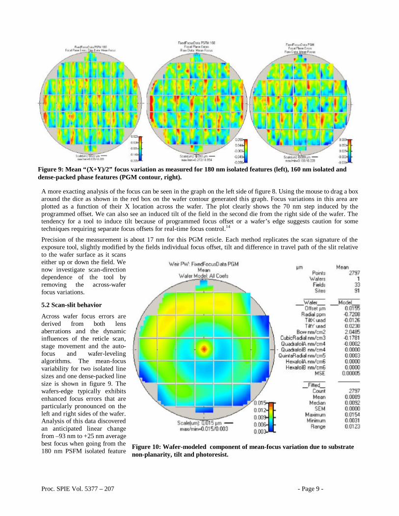
Across wafer focus errors are derived from both lens aberrations and the dynamic influences of the reticle scan, stage movement and the auto-focus and wafer-leveling algorithms. The mean-focus variability for two isolated line sizes and one dense-packed line size is shown in figure 9. The wafers-edge typically exhibits enhanced focus errors that are particularly pronounced on the left and right sides of the wafer. Analysis of this data discovered an anticipated linear change from –93 nm to +25 nm average best focus when going from the 180 nm PSFM isolated feature

Figure 9: Mean “(X+Y)/2” focus variation as measured for 180 nm isolated features (left), 160 nm isolated and dense-packed phase features (PGM contour, right).

Figure 10: Wafer-modeled component of mean-focus variation due to substrate non-planarity, tilt and photoresist.

Proc. SPIE Vol. 5377 – 207 - Page 10 -

to the dense-packed PGM response.

Wafer planarity and photoresist deposition can also influence focus uniformity across the wafer. Weir PSFM was used with the PGM reticle raw data, plotted in the right side of figure 9 to model the wafer induced focus variations shown in figure 10. PSFM data is similar and is therefore not presented in this report.

The wafer planarity is shown to range only a total of 12.3 nm, a significant portion of this being contributed by the cubic-radial deposition pattern exhibited as concentric rings in the figure. Wafer tilt, relatively small in this instance, can be a significant contributor to the loss of depth-of –focus in the process and is separately corrected from the field tilt.

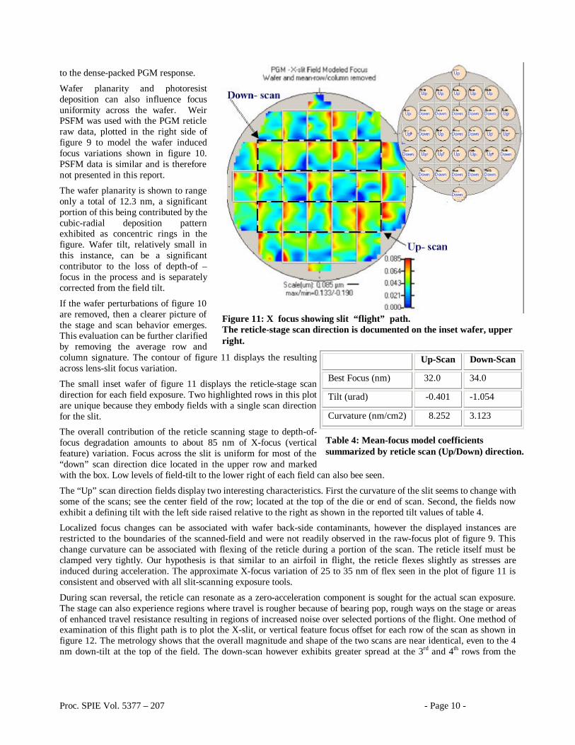
If the wafer perturbations of figure 10 are removed, then a clearer picture of the stage and scan behavior emerges. This evaluation can be further clarified by removing the average row and column signature. The contour of figure 11 displays the resulting across lens-slit focus variation.

The small inset wafer of figure 11 displays the reticle-stage scan direction for each field exposure. Two highlighted rows in this plot are unique because they embody fields with a single scan direction for the slit.

The overall contribution of the reticle scanning stage to depth-of-focus degradation amounts to about 85 nm of X-focus (vertical feature) variation. Focus across the slit is uniform for most of the “down” scan direction dice located in the upper row and marked with the box. Low levels of field-tilt to the lower right of each field can also bee seen.

The “Up” scan direction fields display two interesting characteristics. First the curvature of the slit seems to change with some of the scans; see the center field of the row; located at the top of the die or end of scan. Second, the fields now exhibit a defining tilt with the left side raised relative to the right as shown in the reported tilt values of table 4.

Localized focus changes can be associated with wafer back-side contaminants, however the displayed instances are restricted to the boundaries of the scanned-field and were not readily observed in the raw-focus plot of figure 9. This change curvature can be associated with flexing of the reticle during a portion of the scan. The reticle itself must be clamped very tightly. Our hypothesis is that similar to an airfoil in flight, the reticle flexes slightly as stresses are induced during acceleration. The approximate X-focus variation of 25 to 35 nm of flex seen in the plot of figure 11 is consistent and observed with all slit-scanning exposure tools.

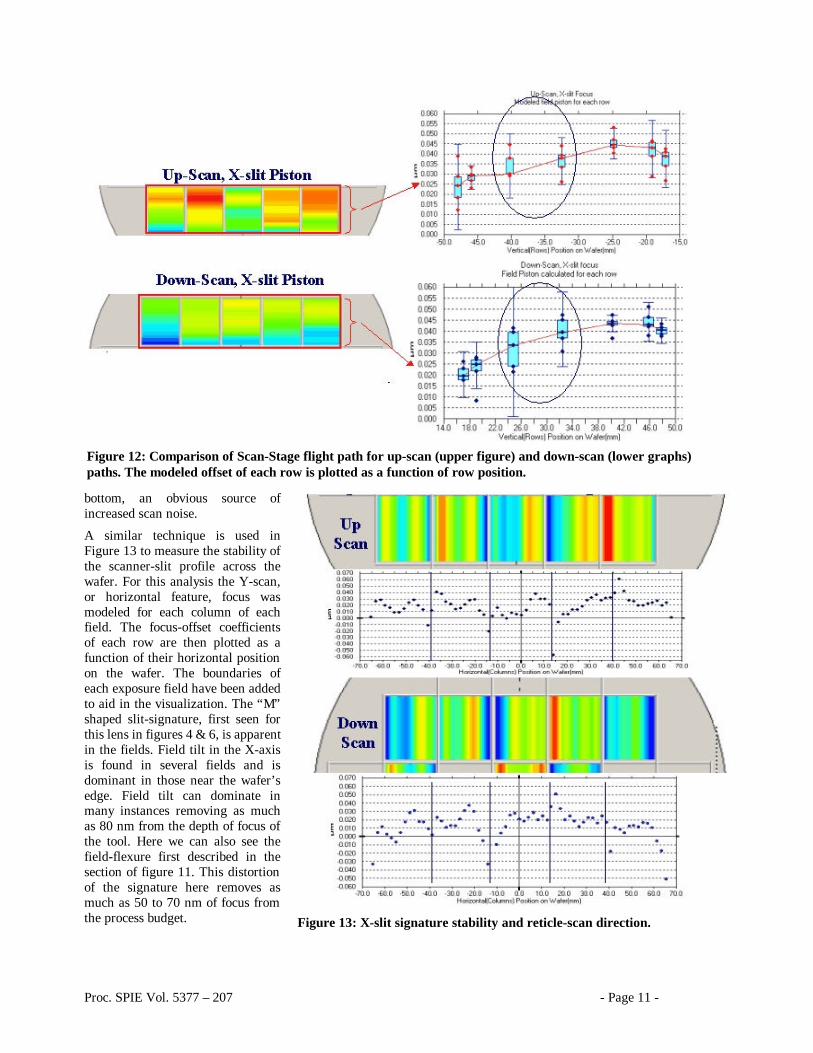
During scan reversal, the reticle can resonate as a zero-acceleration component is sought for the actual scan exposure. The stage can also experience regions where travel is rougher because of bearing pop, rough ways on the stage or areas of enhanced travel resistance resulting in regions of increased noise over selected portions of the flight. One method of examination of this flight path is to plot the X-slit, or vertical feature focus offset for each row of the scan as shown in figure 12. The metrology shows that the overall magnitude and shape of the two scans are near identical, even to the 4 nm down-tilt at the top of the field. The down-scan however exhibits greater spread at the 3rd and 4th rows from the

Figure 11: X focus showing slit “flight” path. The reticle-stage scan direction is documented on the inset wafer, upper right.

Up-Scan Down-Scan

Best Focus (nm) 32.0 34.0

Tilt (urad) -0.401 -1.054

Curvature (nm/cm2) 8.252 3.123

Table 4: Mean-focus model coefficients summarized by reticle scan (Up/Down) direction.

Proc. SPIE Vol. 5377 – 207 - Page 11 -

bottom, an obvious source of increased scan noise.

A similar technique is used in Figure 13 to measure the stability of the scanner-slit profile across the wafer. For this analysis the Y-scan, or horizontal feature, focus was modeled for each column of each field. The focus-offset coefficients of each row are then plotted as a function of their horizontal position on the wafer. The boundaries of each exposure field have been added to aid in the visualization. The “M” shaped slit-signature, first seen for this lens in figures 4 & 6, is apparent in the fields. Field tilt in the X-axis is found in several fields and is dominant in those near the wafer’s edge. Field tilt can dominate in many instances removing as much as 80 nm from the depth of focus of the tool. Here we can also see the field-flexure first described in the section of figure 11. This distortion of the signature here removes as much as 50 to 70 nm of focus from the process budget.

Figure 12: Comparison of Scan-Stage flight path for up-scan (upper figure) and down-scan (lower graphs) paths. The modeled offset of each row is plotted as a function of row position.

Figure 13: X-slit signature stability and reticle-scan direction.

Proc. SPIE Vol. 5377 – 207 - Page 12 -

Figure 14: Astigmatism and the scan direction. Top: Up-Scan direction of the stage. Bottom: Down-Scan variation in astigmatism.

5.3 Astigmatic changes with scan direction

In section 4.3 we first addressed the topic of Lithographers Astigmatism and its variation across the scan-slit. The base concept of a scanner is to increase the NA of the lens in the scan direction and simultaneously average across-slit lens aberrations for each columnar point in the slit. Ideally Astigmatism = (Yscan-Xslit) focus should not change from the top to the bottom of the field. The plotted values of figure 14 however demonstrate that the astigmatism values do change and the changes can be sensitive to the direction of scan.

The up-scan direction maintains its characteristic on this tool for being the quieter of the two scans by varying in mean astigmatic behavior by on 10 nm at the bottom of the scan. A small 5 nm upswing is also visible at the end of scan. The down-scan direction exhibits the same 5 nm astigmatic behavior at the start of scan and then, in the 3rd row from the end, rebounds in a 10 nm upswing at the end of scan.

6. CONCLUSIONS

Multiple methods of measuring focus are available to the technologist. Lens-derived focus errors can be derived using focus-matrix analyses. Stage and scan induced errors can only be fully analyzed using a full wafer exposure of fields conducted with a fixed exposure tool focus. Of the four methods investigated, only the PSFM and PGM technologies provided a capability for fixed-focus analysis.

7. REFERENCE 1 International Technology Roadmap for Semiconductors (ITRS), http://public.itrs.net. 2 B. La Fontaine, M. et al, “Analysis of Focus Errors in Lithography using Phase-shift monitors”, Proc. SPIE, Vol 5040-47, (2003) 3 S. Stalnaker et al., “Focal plane determination for sub-half micron optical steppers”, Microelectronic Engineering 21 (1993), p.33. 4 J. W. Bossung, “Projection Printing Characterization”, Developments in Semiconductor Microlithography II, Proc. SPIE(1977) Vol. 100, pp. 80-84 5 M.A.Zuniga, G.M.Wallraff, A.R.Neureuther, Proc. SPIE 2438 (1995) 6 T.A. Brunner, “New focus metrology technique using special test mask”, OCG Interface ’93, Sept. 26, 1993, San Diego, CA. Reprinted in Microlithography World, 3 (1) (Winter 1994) 7 “Image Sensor System”, ASML PAS 5500 System Introduction 4022-502 – 43124, pp,. 77-81, 1995 8 J. Kirk et al, “Aberration measurement using in situ two-beam interferometry”, Proc. SPIE Vol. 4346 (2001) pp. 8 to 14.

9 W. Roberts, G. Kunkel, “Optimization and characterization of the Blazed Phase Grating focus Monitoring Technique”, Proc. SPIE, Vol 5377-206 (2004). 10 B. La Fontaine, M. et al, “Analysis of Focus Errors in Lithography using Phase-shift monitors”, Proc. SPIE, Vol. 5040-47, (2003) 11 H. Nomura, “New phase shift gratings for measuring aberrations”, Proc. SPIE Vol. 4346 (2001) pp 25-35. 12 M. Moers et al, “Application of the aberration ring test (ARTEMIS™ ) to determine lens quality and predict it’s lithographic performance”, Proc. of SPIE Vol 4346 (2001) pp. 1379 to 1387. 13 A.Y.Abdo et al, “Equivalent modeling technique for predicting the transient thermomechanical response of optical reticles during exposure”, Proc. Of SPIE vol 537-151 (2004) 14 C. Ausschnitt, C. Progler, W. Chu, “CD control of low k-factor step-and-scan lithography”, Proc. SPIE Vol 4346 (2001), pp. 293 – 302.