creating firewall rules with machine learning techniques

Creating firewall rules with machine learning

techniques

Author:Roland Verbruggen, Student at Kerckhoffs institute [email protected]

Supervisor:Tom Heskes, Radboud Universiteit Nijmegen

Abstract

The war against cybercrime is a constant battle. While cybercriminals keep using the same basic attack techniques [M.v.j.], the amountand diversity of malware grows [M. Fossi]. This renders security defensesineffective such that millions of computers are infected with malware inthe form of computer viruses, internet worms and Trojan horses. Thesecybercrimes cost the society money [G. Lovet, M. Clement, C. Kanich]and are a threat to our privacy. Intrusion detection is a critical compo-nent when fighting cybercrime in the area of network security. Intrusiondetection systems (IDS) look at characteristics of network packets or se-ries of packets to determine whether the packets are malicious or not. Thegoal of this thesis is to show how better and more complex firewall rulescan be created with the use of machine learning algorithms. These newfirewall rules contribute to better computer intrusion detection systems.This thesis looks at existing machine learning methods such as randomforests [L. Breiman] and neural networks [K. Hornik] and how firewallrules can be extracted from the resulting models. The models are trainedand tested on a novel labeled network data set containing malicious andnormal packets. This data set was created for this thesis and has not beenused before. How the data set is created is also presented in this thesis.However, as machine learning techniques work well on networks with sim-ilar traffic such as SCADA networks, a special chapter in Appendix A isincluded to this thesis on SCADA networks.

1

Contents

1 Introduction 41.1 Motivation . . . . . . . . . . . . . . . . . . . . . . . . . . . . . . 41.2 Our contributions . . . . . . . . . . . . . . . . . . . . . . . . . . . 41.3 Organisation of this thesis . . . . . . . . . . . . . . . . . . . . . . 5

2 Machine learning methods 62.1 Multilayer perceptron . . . . . . . . . . . . . . . . . . . . . . . . 62.2 Decision tree . . . . . . . . . . . . . . . . . . . . . . . . . . . . . 9

2.2.1 Random tree . . . . . . . . . . . . . . . . . . . . . . . . . 102.2.2 Random forests . . . . . . . . . . . . . . . . . . . . . . . . 10

3 Methodology 113.1 Creating the data set . . . . . . . . . . . . . . . . . . . . . . . . . 123.2 Feature extraction of data . . . . . . . . . . . . . . . . . . . . . . 13

3.2.1 N-grams . . . . . . . . . . . . . . . . . . . . . . . . . . . . 153.2.2 Dimensionality . . . . . . . . . . . . . . . . . . . . . . . . 163.2.3 Clustering . . . . . . . . . . . . . . . . . . . . . . . . . . . 173.2.4 Combined packets . . . . . . . . . . . . . . . . . . . . . . 17

3.3 Train model . . . . . . . . . . . . . . . . . . . . . . . . . . . . . . 183.4 Test model . . . . . . . . . . . . . . . . . . . . . . . . . . . . . . 19

3.4.1 Percentage split . . . . . . . . . . . . . . . . . . . . . . . . 193.4.2 Cross validation . . . . . . . . . . . . . . . . . . . . . . . 193.4.3 Confusion matrix . . . . . . . . . . . . . . . . . . . . . . . 20

3.5 Visualize model . . . . . . . . . . . . . . . . . . . . . . . . . . . . 20

4 Data sets 214.1 The motivation for creating the data set . . . . . . . . . . . . . . 214.2 Data sets . . . . . . . . . . . . . . . . . . . . . . . . . . . . . . . 21

5 Performance evaluation 245.1 Depth of random tree . . . . . . . . . . . . . . . . . . . . . . . . 245.2 Neural networks . . . . . . . . . . . . . . . . . . . . . . . . . . . 245.3 Grouped packets . . . . . . . . . . . . . . . . . . . . . . . . . . . 255.4 Jripper . . . . . . . . . . . . . . . . . . . . . . . . . . . . . . . . . 26

6 Resulting rules 28

7 Conclusion 30

Appendices 31

2

A Creating firewall rules for SCADA networks 31A.1 Introduction . . . . . . . . . . . . . . . . . . . . . . . . . . . . . . 31

A.1.1 SCADA . . . . . . . . . . . . . . . . . . . . . . . . . . . . 31A.1.2 Number of SCADA systems connected to the Internet . . 31

A.2 Obtaining the data set . . . . . . . . . . . . . . . . . . . . . . . . 34A.3 Sample attack (Kingview) . . . . . . . . . . . . . . . . . . . . . . 35A.4 Project determination and specification . . . . . . . . . . . . . . 36

B List of abbreviations 38

C Summary of send documents (21 july) 39

D Application of machine learning technique for ArcSight 40D.1 Introduction . . . . . . . . . . . . . . . . . . . . . . . . . . . . . . 40D.2 The machine learning and visualisation method . . . . . . . . . . 40D.3 The resulting firewall rules in ArcSight . . . . . . . . . . . . . . . 42D.4 Remarks . . . . . . . . . . . . . . . . . . . . . . . . . . . . . . . . 43

E Visualised experiments 44E.0.1 Experiment 0 . . . . . . . . . . . . . . . . . . . . . . . . . 44E.0.2 Experiment 1 . . . . . . . . . . . . . . . . . . . . . . . . . 44E.0.3 Experiment 2 . . . . . . . . . . . . . . . . . . . . . . . . . 44E.0.4 experiment 3 . . . . . . . . . . . . . . . . . . . . . . . . . 45

E.1 Experiment 4 . . . . . . . . . . . . . . . . . . . . . . . . . . . . . 45E.1.1 experiment 6 . . . . . . . . . . . . . . . . . . . . . . . . . 47

E.2 Experiment 7 . . . . . . . . . . . . . . . . . . . . . . . . . . . . . 47E.3 Experiment 8 . . . . . . . . . . . . . . . . . . . . . . . . . . . . . 48

3

1 Introduction

This chapter explains how machine learning techniques can help in the area ofIDS and motivates the development of IDS systems.

1.1 Motivation

Secure computer systems should assure the following services: integrity, authen-tication, non-repudiation, confidentiality and availability[A. Simmonds]. In-tegrity assures that no cyber criminals change data that is stored on computersystems or being transmitted between computers. Confidentiality assures thatno information is disclosed to unauthorized people. Availability assures thatthe information on a network can be requested if it is needed. If cyber criminalsviolate these services this costs our society money. It is hard to estimate howmuch money because it is hard to see what costs need to be taken into accountand what costs should not be taken into account: there is no framework toaccess the economic costs [M. Eeten]. What also makes it harder to estimatethe costs is that corporations do not like to make it public when they sufferfrom computer intrusions [B. Cashell]. However, cost estimates have been made[G. Lovet, M. Clement, C. Kanich]. A report of McAfee reports that the globalcybercrimes costs range from $300 billion to $1 trillion and from $ 24 billion to$120 billion in the US alone [McAfee].

Intrusion detection systems are needed to put a stop to cyber attacks. Thesesystems require a model of intrusion: what should the IDS look for? This modelthat distinguishes between an attack and normal data is created with machinelearning techniques. Research on computer security with machine learning algo-rithms has been done before, for example, by Konrad Rieck [K. Rieck]. Othershave tried to discover patterns or features that can be used to recognize anoma-lies and known intrusions [S. Mukkamala]. Using machine learning algorithmsto detect intrusions has several advantages; zero-day malware can be detectedthrough statistical analysis of previous examples. Machine learning can alsohelp data analysts to analyze large amounts of data by classifying programsor data in groups that might be malicious or not. Traditionally data analystslooked at patterns in connections from certain IP addresses with histories ofintrusive behavior. However, intrusions have become more complex. For ex-ample, intrusions can be low and slow which means that an attack consists ofintrusive behavior over hours, days or weeks and they can have more than onenetwork source. Machine learning can be used to help the data analyst by doingcomplex pattern recognition. Automating this work has the advantage that itcan monitor and correlate large numbers of intrusive signatures or patterns.

1.2 Our contributions

This thesis contributes to the war against cybercrime. This is done by creatingmore complex firewall rules with the use of machine learning algorithms. Thispaper contributes by giving insight in how to use machine learning algorithms

4

to create these better firewall rules. This method is novel in the sense of howthe dataset is created on which the machine learning algorithms are applied.How the data set is created is also described in this paper.

The goal of this thesis is to to create a model using machine learning tech-niques that can differentiate between malicious and normal network traffic, ex-tract a set of rules from this model and then extract useful firewall rules fromthis set. The model can not directly be used in a real environment or as afirewall because it is unrealistic to assume that a model can be created of whichthe false positive rate of this model is low enough while still having a good truepositive rate. The research Question therefore is:

Can one use machine learning techniques to build a model that differentiatesbetween malicious and normal traffic, extract a set of rules from these modelsand then create useful firewall rules from this set that can be used in a realenvironment?

This question is answered by creating the model, testing its performance,extracting a set of rules and investigating these rules.

1.3 Organisation of this thesis

The introduction of this thesis explains why it is important to invest in computerintrusion detection systems and briefly motivates the goal of using machinelearning methods to automate intrusion detection. The research question isalso introduced in the first chapter. Chapter 2 describes the machine learningmethods that are being used in this thesis. The third chapter describes themethodology for achieving the answer of the research question. In particular,it explains how the data set is created and how to apply the machine learningmethods. The fourth chapter describes the data sets that are used to train andtest the models on. The experiments that are run on the data set and theirresults are given in chapter 5. The empirical evaluation and the conclusionsof the experiments are also presented in chapter 5. In chapter 6 the resultingfirewall rules are given. The conclusions are discussed in Chapter 7. AppendixA suggests to create firewall rules for SCADA networks with machine learningtechniques. Appendix D contains visualisations of models that resulted fromthe machine learning techniques.

5

2 Machine learning methods

Machine learning concerns the construction of systems that can learn from data.A broad definition of machine learning is given by [M. Tom]: ”A computerprogram is said to learn from experience E with respect to some class of tasksT and performance measure P , if its performance at tasks in T , as measured byP , improves with experience E.” In our case a machine learning system learnsto distinguish between malicious and normal network traffic.

Its performance gets increased each time it trains on another example orinstance during the training phase. Inputting a training instance can be seen asan experience. There are various kinds of machine learning methods. Machinelearning can be supervised or unsupervised. If it is supervised the data thatthe computer program learns form is labelled. In other words, the computerprogram can learn from examples with the right answer. If the data does nothave labels this means that the data does not contain the class to which theinstance belongs. This is also called clustering. In our research the data islabeled, so it is a supervised machine learning task. In the subsections belowsome supervised machine learning approaches are discussed.

2.1 Multilayer perceptron

A multilayer perceptron (MLP) or neural network is a computational modelthat consists of interconnected perceptrons or nodes that can recognize pat-terns. Warren McCulloch and Walter Pitts were the first (1943) to create acomputational model for neural networks based on mathematics and algorithms[S. Warren]. An MLP consists of at least 2 columns of nodes. On the first col-umn the input is clamped and the last column outputs the results.The outputneuron that has the biggest output is the class to which the input is classified.Each node is fully connected to all nodes in the column after it, the connectionsbetween them have weights. An MLP learns by adjusting these weights w. Anetwork with only 2 column is called a pattern associator (PA). The PA is alinear classifier. When the PA is working correctly the output unit j linked tothe correct class should have the highest activation. The activation a is calcu-lated by taking the net-input n through sigmod function where the net input nis the sum of the input units i, times its weight w:

aj =1

1− e−naj

where

naj =

i∑1

ai ∗ wij

A PA cannot solve all input patterns. For example, the XOR-problem cannotbe learned by the PA [M. Eldracher]. A multilayer perceptron network is usedin this thesis. This is different from a pattern associator in the sense that it

6

has one or more hidden layers: the multilayer perceptron network has at least3 columns of nodes. This network can learn the XOR-problem.

Before the MLP network is capable of linking the input data to the correctclass, the correct weights should be determined. This is done by training thenetwork with the supervised data set and updating the weights. How this worksis explained with just one hidden layer. The learning process in an MLP is calledback propagation. Back propagation has three stages:

1. Forward propagation. The network calculates the output o by subse-quently computing:

The activation of the hidden units k

ak =1

1− e−nak

where

nak =

k∑i=1

ai · wik

oj =1

1− e−naj

where

naj =

j∑i=1

hk · wkj

This is illustrated in figure 1:

Figure 1: Illustration of forward propagation

2. Backward propagation

In the back propagating phase the learning takes place. The weights learnthrough the error e (= activation Output o minus the desired outcome t (thetarget) computed at the output layer:

e = o− t

The weight is then changed by e times the activation output aj times the acti-vation of the hidden neuron hk. e Is a variable is a variable defined by the user.If it is higher it trains faster but it could jump over a global optimum.

∆wkj = e · aj · hk

7

3. Update weights

The new weight will become:

wkj = wkj + ∆wkj

The learning will stop after some termination criteria (a number of epochsfor example) or when certain recognition performances have been reached.

As mentioned earlier the MLP is good at being able to learn not only fromlinear but also nonlinear data. A quote from Hornik: ”The MLP is capable ofapproximating any measurable function to any desired degree of accuracy, in avery specific and satisfying sense.” [K. Hornik]. Hornik even goes as far as callingthe MLP a universal approximator. The MLP also has disadvantages. For one,there are difficulties in implementing and training the network [M. W. Gardner].For example a common mistake is leaking information from the test set to thetraining set. Creating easy to use programs might solve this problem or makeit easier but background knowledge of MLP is still required when using MLP’s.Another disadvantage of the MLP is the difficulty of interpreting the MLP. Theresulting model of the training phase is complex and it is hard to see why certaininstances are classified into a certain class. There do however exist visualizationmethods for MLP’s [F. Piekniewski].

The last disadvantage of the MLP classification method is the complexityof the classification process. Using an MLP in combination with large datasets requires alot of time to perform classification. Below the complexity of theforward propagation of the MLP is evaluated.

First the node net-input needs to be computed. The complexity of this is2dn where d the number of training instances and n the number of features.The number of features is also the amount of input neurons.

Then the input is evaluated, this is done by activating each node in eachlayer. The complexity of the node activation is:

d

N∑s=2

Ps

where Ps is the number of nodes at layer s. The activation of the nodes generatesoutput. This needs to be evaluated. This is done with a residual evaluation.The residual evaluation gives simply the distance between the right outcome andthe outcome given by the model. This needs to be calculated for each outputnode and for each training instance. The complexity of this is dPN . We alsoneed to calculate the Error. The complexity of Calculating the SSE is: 2dPN

The complexity of residual evaluation is dPN . The complexity of the backwardpass is also primarily dependant on the number of instances, the number offeatures and the number of nodes [E. Mizutani]. So when using large data setswith a large amount of features, this gives problems. Also using large amountsof hidden units in the MLP increases the complexity drastically.

8

2.2 Decision tree

Next to MLPs also decision trees were used to learn patterns from the networkdata. The decision tree takes as input the attributes of the messages and returnsa ”decision” - the predicted output value for the input. The input values canbe discrete or continuous, this is an advantage over the MLP where the inputcannot be continuous. The decision tree makes its decision by performing asequence of tests. Each node in the tree corresponds to a test of the value ofone of the attributes. The values of the leaves of the tree are returned andrepresent the class to which the instance belongs.

The basic idea behind decision tree learning is to test the most importantattribute first. The most important attribute is the attribute that makes thebiggest difference to the classification of a sample, put in other words, the at-tribute that has the highest information gain. The measure for information gainis called entropy. If an instance can be classified into C different values, thenthe entropy of S relative to this c-wise classification is defined as:

Entropy(S) =

c∑i=1

P i log2 pi

where pi is the proportion of instance S belonging to class i and the logarithmis base 2. [M. Tom].

By testing the most important attributes it is hoped that one gets the rightclassification with a small number of tests (small tree). As mentioned before,one advantage is that input values can be discrete or continuous. The outputvalues of the decision tree are discrete. Another advantage is that decision treesare robust to errors. The training data may contain missing attribute values. Achallenge in decision trees is determining the depth of the decision tree. If thetree becomes too large and the depth to high the tree is overfitted on the trainingdata. If there is some noise in the data or when the number of training examplesis too small to be representative for the real data set the overtrained model willnot perform well on real data. The solution would be to stop at the correcttree size or stop the training early. The correct tree size could be determinedby using separate data from the training data to evaluate the decision tree.This technique was also used in this research and is also called training andvalidation set approach. A simpler solution that was also used in this researchis to determine a maximum depth to which one lets the decision tree expandor use another explicit measure to measure the complexity of the tree and haltat a certain threshold. Another option would be to use a statistical test toestimate whether the expanding of a particular node will improve the decisiontree. For example, the chi-square test can be used. This method was not usedin this research. Choosing the shortest decision tree for the observed data isalso in line with Occams Razor. Occams Razor is a principle that states thatamong competing hypotheses (decision trees), the hypothesis with the fewestassumptions should be selected [A. Blumer].

The learning algorithms differ for each technique and will be discussed below.

9

2.2.1 Random tree

A Random decision tree is a decision tree where the input is not only the in-stances but also some random vector Ok. An example of a random tree is usingsplit selection where at each node the split is selected at random from among theK best splits. Another approach to introduce randomness is to use bagging. Ifone has a training set S of size N , one creates m new training sets Si each of sizeN . These subsets Si are created by taking samples from D. It is possible thatthere are duplicate elements in the subsets. Bagging has several advantages.Bagging works good when there is classification noise [T. Dietterich]. Classifi-cation noise means that a small amount of the labels are wrong. Bagging alsohelps to avoid overtraining, this is shown in section 2 of [L. Breiman].

2.2.2 Random forests

A random forest is an ensemble of multiple random decision trees, in otherwords, a bag of random trees. In our setup we used an ensemble of 10 randomtrees. Each random tree in the forest is fully grown (no pruning). The definitionof a random forest is given by Breiman [L. Breiman]: ”A random forest is aclassifier consisting of a collection of tree structured classifiers h(x,Ok), k = 1, ...where the Ok are independent identically distributed random vectors and eachtree casts a unit vote for the most popular class at input x.”

The output of all trees is combined with a combination rule. One exampleof such a combination rule is majority voting. In majority voting, for eachinstance, the majority voting rule lets each classifier classify it into a class. Itthen just outputs the class that most of the trees classified it into. An advantageof majority voting is that it is straightforward.

10

3 Methodology

The methodology of this thesis is explained in the following six steps:

1. Create data

2. Feature extraction of data

3. Combine data

4. Train model

5. Test model

6. Visualize and interpret results

The methodology that is explained in this chapter is depicted in figure 2.

Figure 2: Based on the generated data mathematical models are created thatcan classify packets. These models can also be visualized. From these visualizedmodels firewall rules can be created.

The main advantage of the machine learning methodology used is that at-tacks and exploits similar to the ones used in Kali [Kali] or Metasploit [Metasploit]will be detected. Another advantage is that the packets that are similar to nor-mal data will not be marked as an attack thus reducing false positives. It issuspected that many attacks these days are run with tools like Kali or Metas-ploit. If the attack is not performed by a tool the chance is big that the attackis an altered existing attack from Kali or Metasploit or a similar tool.

11

3.1 Creating the data set

One way data is created is by placing 2 computers next to each other on aLAN and generating traffic. The attacking computer that is running Kali iscalled the attacking machine and the computer that is being hacked is calledthe target machine. The traffic generated needs to be both normal traffic andmalicious traffic. To achieve this a specific setup was used. On one laptopthe special hacking operating system Kali Linux was installed. This operatingsystem contains the Metasploit framework that contains over 1,200 exploits andan average of 1.2 new exploits are added every day. These exploits can beexecuted against the target machine. In order for the exploits to work, certainservices and programs that contain vulnerabilities need to be running on thetarget machine. For this, Metasploitable 2.0 is used. A list of some of thevulnerabilities of Metasploitable 2.0 can be read here [vulns]. Some examplesof vulnerable applications that run on Metasploitable 2.0 are phpMyAdmin,tikiwiki and webdav.

During the attack of the attacking machine on the target machine, all net-work data is logged on the target machine. This is done by making tcpdumps[tcpDump] on the target machine. tcpdump is a command in unix that capturesall network traffic from a specified ethernet adapter. By setting the -s flag to 0we make sure that we capture the whole packet (65535 bytes is the maximumsize of a packet). When all attacks are run and the PCAP file is created thatcontains all packets, the PCAP file is loaded into Wireshark to visualize andinspect the data. Wireshark is also used to filter out everything but TCP/IPtraffic: all traffic that is not TCP/IP is thrown away. A sample of resultingdata is shown in figure 3.

Figure 3: Sample of 38 TCP packets in Wireshark

The normal data is generated by normally using the target machine andperform activities such as web-browsing, downloading files, and e-mailing. Inthis case the pcap files containing the packets are also created using the tcpdump

12

command.

3.2 Feature extraction of data

The network traffic that is captured consists of packets. They can be seen asletters being send over a network. These packets also have things like an addressand sender. Information like the address, sender, the time the packet was sentand the time to live are in header information. We want to separate the headerinformation from the actual message of the packet. The actual message of apacket is called the payload. Figure 4 displays one packet. In the top of theimage one can see all the header information and the payload starts with theblue selected text GET. The blue selection matches the hexadecimal selectedbytes and with the corresponding ASCII characters that these bytes represent:47 45 54. In the ASCII figure 5 we can see that the hexidecimal numbers 47,45 and 54 indeed correspond to the capital letters G,E and T.

Figure 4: Sample of a single Packet

13

Figure 5: ASCII table (Not all 256 bytes but only until 127), Source:[LookupTables]

One way features are extracted from the payload of the packet is by countingthe frequency of each possible byte. This is also called a bag of bytes. Moreadvanced methods for the feature extraction are possible and will be explainedbelow. There are 256 possible bytes so that gives 256 numerical features. Next tothe features a label is added to specify to which class a packet belongs (maliciousor normal). The actual extracting of the payload of the packets and the countingof the bytes is done in a JAVA program. This Java program uses the winpcaplibrary to be able to read in pcap files [Winpcap].

Next to these 256 features other features are extracted from the packet:

• Len: total length of packet

• Length: length of header

• Caplen: amount of actual data which was stored

• Ident: identifier

• Flag: flagged true or false

14

• StdevTime: The standard deviation of the time the packet itself was re-ceived and the last 7 packets send before it. It is a measure of the amountof variation or dispersion there is between the times of the last 8 receivedpackets.

3.2.1 N-grams

A more advanced method to extract features from packets is to use n− grams.In this case a Packet has many features; one for each possible n − gram. Ann − gram is a contiguous sequence of n bytes. The value of the feature is thefrequency of occurrence of that n − gram. For example, of the 6 consecutivebytes (hexadecimal coding) 00, 01, 02, 03, 04, 05 the 2-gram is 00 01, 02 03, 0405 and the 3-gram is 00 01 02, 03 04 05. Not only n− grams are used but alsoskip grams or n−v−grams. The difference here is that a space v is left betweeneach pair of bytes. One can imagine this as if a v+2 long sliding window witha gap of length v between the first and last byte that goes over the bytes of thepayload. This is illustrated in figure 6 and 7; the pictures are a representationof the payload of a packet.

Figure 6: The sliding window moves on one step and sees ”47, 20”. So thefrequency of that skip gram is increased with one.

15

Figure 7: The sliding window sees the 2-2-gram ”45,2f”. So the frequency ofthat skip gram is increased with one.

3.2.2 Dimensionality

The reason that gaps were used between the bytes is because the amount offeatures and thus dimensionality greatly increases with n and it is wanted toextract structural information. The amount of possible features grows exponen-tially with n. By using a gap v it is still possible to extract some informationrelated to the n− grams, with n >2. With n = 2 the amount of dimensions isstill large (65536). This means that the frequency matrix will also be that large.The frequency matrix will have a lot of zero values because a lot of skip gramswill not occur in the payload. Another common use of n−grams and frequencymatrix is in document classification, were documents are classified into cate-gories based on n − grams (word pieces in the document). It has been shownthat even if they have to deal with very large amounts of features (more than10000) and thus more than 10000 dimensions; SVM classifiers still work for textcategorization [T. Jaochims]. In this thesis SVMs are used to categorize packetsas malicious or normal. SVM classifiers still work in case of high dimensionalproblems because the documents are very sparse and only the n− grams thatoccur in the document are considered. You could effectively process feature vec-tors of 10 000 dimensions, given that these are sparse. Even though skip gramsare used, our feature space is big. The dimensionality of the feature space can

16

be reduced by applying a clustering algorithm. The cluster algorithm used is aclustering algorithm proposed by Dhillon et al in [I. S. Dhillon]. This clusteringalgorithm is somewhat similar to well-known k-means algorithm [C. Mihaescu].

3.2.3 Clustering

ClusteringThe clustering algorithm uses the following as input:

• The occurrence frequency matrix of skip grams.

• The desired number of clusters k. (This is also the number of featuresthat each item will have after clustering. So this is also the number ofdimensions you will have).

• The tolerable information loss t.

It then initializes random clusters. This just means that each feature israndomly assigned to one of the k clusters. Each feature is then moved fromcluster to cluster until the information loss is less than t. The information loss iscalculated with Kullback-Leibler divergence. The Kullback-Leibler divergenceof Q from P is a measure of the information lost when Q is used to approximateP . KullbackLeibler divergence measures the expected number of extra bitsrequired to code (code to binary) samples from P when using a code based onQ, rather than using a code based on P . The output of the clustering algorithmare the k clusters, where each cluster is the sum of a set of features (addingup the probabilities). The features themselves are cells from the conditionalprobability matrix. Each cell in this matrix is still the conditional probabilitymatrix holds the probability that a skip gram occurs with relation to the targetclass P (X | T ). So each new feature in the new k-dimensional feature space canbe computed in the following way:

P (Sh|f i) =∑

Xj∈Sh

P (X j|f i)

Where h = 1,...,k and P (Sh|F i) is the conditional probability that the set ofskip grams S occurs in file i. If there are ten features, which all have a chanceof 0.1 of occurring in the payload of a packet, and one wants to decrease this to9 features, 2 features have to be put together in a cluster where the chance ofeither of the features occurring is the sum of the 2 features.

3.2.4 Combined packets

Because computer intrusions or attacks over a computer network usually consistof more than one packet it is preferred to use groups of packets. This meansmultiple packets are put into a group and the group of packets is classifiedas malicious or normal. In our case the group consists of only malicious oronly normal packets. Our case is not to be confused with an other method of

17

grouping packets together called Multiple Instance learning [O. Maron] wheregroups can consist of malicious and normal packets and a group is maliciousif one packet of the group is malicious and normal otherwise. How to createthe groups is based on other papers. In [I. Weon] it is suggested to use timerelated and risk related parameters. It is decided to use a simple time relatedparameter: timestamps. A packet is stamped with the time at which it arrivesat the destination machine. This is done by making bags of all packets thatarrived in the first 0.001 seconds, then another bag of all packets in the 0.001seconds after that etc. A disadvantage of this method is that sometimes the bagsonly contain 1 instance because there is only one packet in those 5 seconds. Butnormally the bags are of size of about 8. This was tuned to 8 because in mostdata sets the attacks were also consisting of about 8 packets. As explainedin [I. Weon], many other bag sizes can be used, ranging from 20 to even 50packets. This might be different for each data set but is interesting for furtherinvestigation.

3.3 Train model

The model is trained on the resulting data set. This is a two-class classificationproblem (malicious and normal data). A simple and easy to understand andvisualize way of classifying is to use decision trees. The disadvantage of decisiontrees is that they are not good at obtaining good classification rates and lowfalse positives. In a first attempt the following decision tree was created as asample that can be seen in figure 8.

Figure 8: Sample tree

In the tree every node and leaf is numbered, and behind the number ofthe node and the ”:” is a number indicating which byte is used by that node.The frequency of that byte determines what path through the tree should be

18

followed. This is a simple tree and gives an idea of the technique. However thisdecision tree did give a recognition rate of 91.5%.

Next to decision trees there are many more machine learning techniques tocreate a model. Some examples are a neural network, random trees, randomforest, and many more.

3.4 Test model

In this chapter some validation methods that are used in this research are ex-plained. In order to test the performance of the model, benchmarking methodsare used. In this process, a model is trained and tested using different partitionsof the benchmark data. For each sample of the data, the output hypothesis ofthe model is compared to the corresponding (known) category. It is desired totrain our model on a data set with targets and outliers. The resulting modelshould give as many true positives and true negatives as possible, and as fewfalse negatives and false positives as possible. A false negative occurs if thehypothesis says it should be negative but in fact it is positive (the data sampleis normal data but is wrongly classified as an attack). A false positive occurs ifthe hypothesis says that the data sample is an outlier (attack), whereas in factit is a target (normal). A true positive is when the hypothesis says it should bea positive and it is in fact a positive. A true negative is when the hypothesissays it should be a negative and it is in fact a negative. A model is tested bycounting how many false positives and false negatives there are. As few as pos-sible false positives and false negatives are desired. In the case the model is useddirectly in practice it is very important to have a very low false positive rate ofthe data set because in the kind of data sets that is used there are hundreds orthousands of normal data packets. Even if there is a false positive rate of 0.01%there will still be a lot of false alarms going on.

3.4.1 Percentage split

A model such as a decision tree or MLP is a classifier. It is a function that mapsan unlabelled instance to a label. The validation is often done on a separate partof the (labeled) data set. The easiest validation method is to use a percentagesplit. The original data set is split into a training set and a test set. The model istrained on the train set then the test sets without the labels are inputted into themodel. After the model is trained the output of the model is compared with thelabel and the amount of errors are calculated. The percentage of instances thatare correctly classified is called the recognition rate. The validation methodsneed to measure the accuracy of the model (classifier) so that we can comparethem. Another validation method is the cross validation method.

3.4.2 Cross validation

Cross validation is done in a number of rounds. At each round the data setis split up in a train set and a test set. The model is trained on the train set

19

and then tested on the test set, at each round a different part of the data setis the test set. The rounds are often called folds. For example a 10 fold crossvalidation means splitting the data up in 10 parts and doing 10 rounds. Crossvalidation is also called the ”leave one out method” because at each round youleave one part of the data set out to test on. At the end the average of theperformance of all the rounds is calculated.

Figure 9: Illustration of 4 fold cross validation, also called leave one out.

An advantage of cross validation is that one can test and train the model on alimited amount of data. Another advantage is that your test and training is moreprecise since it was tested and trained on the whole data set. A disadvantageis that at each round a model is trained and tested. The training of the modeltakes time and at the end all but one of these models are discarded.

3.4.3 Confusion matrix

In this thesis the Confusion matrix is also used as a validation method. AConfusion matrix is a matrix where the each row represents the target class towhich a value belongs and each column represent the target class to which itwas classified. In this matrix one can easily see if the model is confusing classes.Figure 10 is an illustration of a small example of a confusion matrix.

Figure 10: Example of small confusion matrix.

If the values on the diagonal are high it means the results are good, if thevalues on the diagonal are low and the other values high it is an indication thatthe classifier did not work well.

3.5 Visualize model

The resulting model can be visualized in the form of a decision tree. A hu-man can interpret the results and decide what rules should be extracted andimplemented into the firewall. The visualised models are given in Appendix D.

20

4 Data sets

All data sets were created with the methodology described in the methodologychapter. In this chapter first the motivation for creating the data set with thismethodology is described. After the motivation for the data set the descriptionsof specific data sets are given.

4.1 The motivation for creating the data set

Before one can create an intrusion detection model data is needed. Data isoften hard to obtain because of privacy issues. Not many corporations want toshare network traffic data. Network packets often contain private information.Especially labeled data is hard to obtain because labeling the data is laborintensive. Half of the work of this thesis is creating the labeled data set. Aquote:

It is very difficult and expensive to obtain a labeled data set thatis representative of real network activates and contains both normaland attack traffic

[J. McHugh].

Obtaining network traffic from a network is hard because not many corporationswill want to give data. Other researchers also have trouble with obtaining thesedata sets. Papers nowadays still discuss data sets that are from the year 1999and older. The most used data set is the DARPA data set [DARPA]. This dataset is from 1999. Of course this 15 year old data set is outdated. The normaltraffic is not representative for traffic of these days, also the data of attacks isoutdated because different attacks are used these days. Many papers still usethis data set. An example of a paper of 2014 that still uses this data set is[K. Rajitha]. Next to the DARPA data set there is also the KDD Cup data set[KDDcup]. The KDD Cup data set is a subset of the DARPA data set. A paperfrom 2011 that still used this data set is [J. Jonathan], there are even paperspublished in 2013 and 2014 that use the 1999 KKD cup data set to test modelson. Fore example [P. Ahmed], [S. Kumar], and [U. Subramanian]. Many moreof these papers can be found, this shows the need of a new data set and howdifficult it is for researchers to obtain these data sets.

4.2 Data sets

All data sets consist of 1876 maliciouse packets and 11444 normal packets. Indata sets 1,2,3 and 4 the feature extraction of the packets were done with uni-gram. The unigrams give 256 features. In data set 1 the amount of millisecondsthe packets needs to travel, the source port and the destination port were addedas a feature. Data set 2 was the same as data set 1 but the following featureswere added:

• len: total length of packet

21

• length: length of header

• caplen: amount of actual data which was stored

• ident: identifier

• flag: flagged true or false

Data set 3 is the same as data set 2 but the source port and destinationport features were removed. Also a new feature was introduced: the standarddeviation of the time between the last 8 packets that were received. This givesinformation of how fast packets were send after each other. Data set 4 usescombined packets. Each row consists of the last eight packets send. In orderto reduce dimensionality not all 256 bytes of each of the eight packets are used.The following features where used for each packet and combined together:

• Bytes 1 and 2

• Bytes 30 trough 63

• Bytes 120 trough 142

• srcPort: source port

• destPort: port destination

• len: length of header

• length: length of packet

• stdevTime: standard deviation between the time of last eight packets

• ident: identifier


• flag: flagged true or false

Data set 5 is special because it uses the skip grams or n grams discussedin chapter 3.2.2. In this data set a gap size of 1 between each combination of2 bytes is used. This results in 256 * 256 = 65536 features, this is too much.Therefore dimensionality reduction is used as described in section 3.2.3. In thisdata set the dimensionality is reduced from 65536 to 260. This is still a highdimensionality for this data set because there are only about 14000 instances.Therefore datas set 6 is created where the dimensionality is reduced from 65536to 45.

Next to the 260 clusters of skip bytes the following features were added:

• srcPort source port

• destPort port destination

22

• len: length of header

• length: length of packet

• stdev: standard deviation of time last 8 packets received


Data set 6 is similar to data set 5 with the only difference that the amountof skip bytes are clustered together to 45 clusters instead of to 260.

Data set 7 is a data set where packets are grouped together. The packetsin a group are either all malicious or all normal. Packets are grouped togetherbased on time. The time between the first and the last packet in a group is nomore than 10000 ms. Also groups are never bigger than 8 packets.

This is not typical multiple instance learning. In the case of multiple instancelearning bags are mixed positive and negative packets and a bag is considerednegative if one packet in the bag is negative.

Just like data set 6 this data set also contains 45 features containing infor-mation of byte frequency’s and the same extra features as in data set 5 and 6such as source port and length.

23

5 Performance evaluation

This chapter describes the performance of various machine learning methodswith different parameters applied to a number of data sets. In each section anumber of experiments, their differences and the performances are discussed.All data sets were created with the methodology described in the methodologychapter. In chapter 4.2 the data sets where also numbered, in this chapter 3is a reference to these data sets with these same numbers. In column three ofeach table the number of the data set used is given.

5.1 Depth of random tree

In the first five experiments random trees were used. The depth parameter Dindicates how many nodes one needs to follow to get from the first node tothe leaf of the tree. In every experiment a different depth was used in orderto investigate the effect of the depth on the recognition rate (rr). A smalldepth generates a smaller tree that is more simple to interpret. A higher depthgenerates a more complex tree with better recognition rates. For example, witha depth of 9 the recognition rate is 99.744%.

nr Method Data set parameter’s rr TP FP0 Random Tree 1 D = 4 94.099% 0.785% 0.035%1 Random Tree 2 D = 9 99.744% 0.997% 0.007%2 Random Tree 3 D = 3 93.210% 0.932% 0.223%3 Random Tree 3 D = 4 94.400% 0.944% 0.157%4 Random Tree 3 D = 5 95.910% 0.959% 0.156%16 Random Forest 6 D = 22 99.825% 0.995% 0.009

Table 1: Performance results of Random Trees. D is the depth of the tree, rrstands for recognition rate.

5.2 Neural networks

In this section neural networks with various parameters and data sets are com-pared. The recognition rate of experiment five is very low. In the confusionmatrix in Appendix E.1 one can see the problem: the model just classified ev-erything as normal data. This is because there is only one hidden layer makingit impossible for the neural network to learn the complex patterns. The recogni-tion rate is still 85.6% and not 50% because there are more normal packets thanmalicious packets in the original data set. In experiment 6 this experiment isrepeated without the indent feature and with 2 extra hidden layers. The higheramount of hidden layers results in a better recognition rate of 98.65%.

From experiment 5 it was learned that the ident attribute weighs very heavy.One can see this as a fault in the data set or as ”cheating”. Ident is probably

24

unique to many instances, this is not what one wants the model to learn, there-fore the ident variable is left out in experiment 6.

In the third column of experiment 5 and 6 it is noted that ”66% of data set3 is used. This just means that 66% of the packets of data set 3 are used. Thisis because neural networks take a long time to train and test and using the fulldata set would take even longer.

In experiment 14,15 and 16 the only difference is the amount of hidden layers.If the number of hidden layers is increased the recognition rate also increases.Experiment 20 was run with 7 hidden layers. 7 was chosen because this is agood trade off between the amount of time needed to train and test the modeland the recognition rate. The difference between experiment 20 and 15 is thedata set. The difference between data set 6 and 7 is that in data set 7 packetsare grouped together. The results of these experiments show that grouping thepackets together this way increases the recognition rate with 0.32%.

nr Method Data set Vars excluded parameter’s rr TP FP5 Neural network 66% of 3 - N = 133, L = 1 85.600% 0.000% 0.055%6 Neural network 66% of 3 ident N = 133,L = 3 98.650% 0.987% 0.077%14 Neural network 6 - N = 27, L = 4 99.051% 0.95% 0.003%15 Neural network 6 - N = 27 , L = 7 99.119% 0.957% 0.003%17 Neural network 6 - N = 27, L = 10 99.149% 0.954% 0.003%20 Neural network 7 - N = 27,L = 7 99.151% 0.992% 0.036%

Table 2: Performance results. N is the number of nodes per hidden layer, Lis the number of hidden layers and D is the depth of the tree, rr stands forrecognition rate.

5.3 Grouped packets

Experiment 19, 20 and 21 were all run on data set 7. In data set 7 packetsare grouped together. In the table 5.3 the results of the learning algorithmsapplied on data set 7 are shown (experiment 13, 15 and 22). Next to the resultsof algorithms applied to data set 7 the results of machine learning algorithmsapplied to data set 6 are also shown. Data set 6 is the same as data set 7 with theonly difference that the packets are not grouped. It can be seen that our way ofgrouping packets together does not increase performance in the case of randomtrees. The performance of the Neural Network is increased in performance with0.32% when packets are grouped together. In the case of the random forestthere is a small increase of 0.001% when packets are grouped together.

25

nr Method Data set Vars excluded parameter’s rr TP FP13 Random tree 6 - D = 9 99.006% 0.956% 0.005%20 Random tree 7 - D = 9 98.970% 0.954% 0.004%15 Neural network 6 - N = 27 , L = 7 99.119% 0.957% 0.003%20 Neural network 7 - N = 27,L = 7 99.151% 0.992% 0.036%22 Random forest 6 - D = 9 99.741% 0.997% 0.01%21 Random forest 7 - D = 9 99.742% 0.997% 0.01%


5.4 Jripper

Experiments 8, 9, 12 and 18 are performed with Jripper. All results are verygood, it appears that Jripper is the best overall performer of all methods tested.The best performance by Jripper is when it is applied to data set 5, here theskip gram is used. The second best is experiment 6, here also skip grams areused, but there are only 45 clusters used instead of 260. It is logically expectedthat when the amount of clusters is reduced the performance is lower becauseone throws information away.

nr Method Data set Vars excluded parameter’s rr TP FP8 Jripper 1 - - 99.804% 0.998% 0.006%9 Jripper 1 src and dest port - 98.678% 0.987% 0.038%12 Jripper 5 - - 99.835% 0.994% 0.001%18 Jripper 6 - - 99.704% 0.985% 0.001%

Table 4: Performance results of Jripper. rr stands for recognition rate.

26

Table 5 shows all the results together.

nr Method data set Vars excluded parameter’s rr TP FP0 Random tree 1 - D = 4 94.099% 0.785% 0.035%1 Random tree 2 - D = 9 99.744% 0.997% 0.007%2 Random tree 3 - D = 3 93.210% 0.932% 0.223%3 Random tree 3 - D = 4 94.400% 0.944% 0.157%4 Random tree 3 - D = 5 95.910% 0.959% 0.156%5 Neural network 66% of 3 - N = 133, L = 1 85.600% 0.000% 0.055%6 Neural Network 66% of 3 ident N = 133,L = 3 98.650% 0.987% 0.077%7 Random tree 4 - D = 3 95.872% 0.987% 0.077%8 Jripper 1 - - 99.804% 0.998% 0.006%9 Jripper 1 src and dest port - 98.678% 0.987% 0.038%10 Neural network 5 - N = 133, L = 3 98.717% 0.947% 0.006%11 Random tree 5 - D = 9 98.975% 0.939% 0.002%12 Jripper 5 - - 99.835% 0.994% 0.001%13 Random tree 6 - D = 9 99.006% 0.956% 0.005%14 Neural network 6 - N = 27, L = 4 99.051% 0.95% 0.003%15 Neural network 6 - N = 27 , L = 7 99.119% 0.957% 0.003%16 Random forest 6 - D = 22 99.825% 0.995% 0.001%17 Neural network 6 - N = 27, L = 10 99.149% 0.954% 0.003%18 Jripper 6 - - 99.704% 0.985% 0.001%19 Random tree 7 - D = 9 98.970% 0.954% 0.004%20 Neural network 7 - N = 27,L = 7 99.151% 0.992% 0.036%21 Random forest 7 - D = 9 99.742% 0.997% 0.01%


27

6 Resulting rules

In this chapter methods are compared and resulting rules that can be drawnfrom the experiments are discussed.

It is clear that more complex models have better recognition rates. Neuralnetworks also work well (the recognition rates are over 98.6%).

After looking at the the images in the Apendix E it appears that the impor-tant ASCII characters are 0, 8, 12, 32, 39, 43, 50, 58, 67, 73, 98, 110, 115, 142,237, 250. With important it is meant that

Some resulting Jripper rules from experiment 8:

(destPort ≤ 56118)and(srcPort ≤ 55177)and(3 ≤ 1)⇒ category = mal(1513.0/0.0)

(0 ≤ 0)and(53 ≤ 3)and(50 ≥ 10)and(47 ≥ 7)⇒ category = mal(101.0/0.0)

(destPort ≤ 55757)and(srcPort ≥ 57277)⇒ category = mal(78.0/0.0)

(destPort ≤ 55757)and(srcPort ≤ 56118)and(0 ≥ 12)⇒ category = mal(87.0/2.0)

(destPort ≥ 57314)⇒ category = mal(36.0/0.0)

(0 ≤ 0)and(58 ≤ 4)and(srcPort ≥ 6667)and(77 ≥ 1)⇒ category = mal(22.0/1.0)

(0 ≤ 0)and(55 ≤ 1)and(87 ≥ 4)and(1 ≤ 0)⇒ category = mal(9.0/0.0)

(srcPort ≥ 8080)and(srcPort ≤ 55757)and(99 ≥ 5)and(132 ≤ 3)⇒ category =mal(13.0/1.0)

Some Resulting Jripper rules from experiment 9:

(0 ≤ 0)and(42 ≤ 0)and(85 ≥ 1)and(46 ≥ 7)and(40 ≥ 1) ⇒ category =mal(1171.0/1.0)

(44 ≤ 0)and(3 ≤ 1)and(10 ≤ 0)and(32 ≥ 1)and(34 ≤ 0) ⇒ category =mal(291.0/5.0)

(123 ≤ 0)and(58 ≤ 5)and(3 ≤ 1)and(115 ≥ 4)⇒ category = mal(111.0/15.0)

(44 ≤ 0)and(3 ≤ 1)and(60 ≤ 0)and(68 ≤ 0)and(0 ≥ 3) ⇒ category =mal(107.0/10.0)

(58 ≤ 1)and(3 ≤ 0)and(255 ≤ 0)and(0 ≤ 18)and(10 ≤ 0) ⇒ category =mal(71.0/10.0)

28

Some resulting Jripper rules from experiment 19:

(23 ≤ 21)and(23 ≤ 5)and(destPort ≤ 56553)⇒ category = mal(1257.0/0.0)

(23 ≤ 23)and(lenght ≥ 315)and(destPort ≤ 56915)⇒ category = mal(147.0/1.0)

(stdevT ime ≥ 14813)and(23 ≤ 17)and(srcPort ≤ 55609)and(0 ≤ 0)and(srcPort ≤6667)⇒ category = mal(106.0/1.0)

Rules can also be created from the models that resulted from the experi-ments. One must first interpet the visualised model, For example, in the result-ing model of Figure 8 one can derive the following rule: If ascii character ”*”occurs less than 0.5 times and character ”H” occurs more than 5 times and the”start of heading” occurs more than 0,5 times the packet is normal.

29

7 Conclusion

The research question was :Can one use machine learning techniques to build a model that differentiates

between malicious and normal traffic, extract a set of rules from these modelsand then create useful firewall rules from this set that can be used in a realenvironment?

The answer to the research question is yes. In this thesis a data set withmalicious and normal traffic was created as described in chapter 3.1. Chapter 3also describes and defines the difference between malicious and normal traffic forthis thesis. After these feature extraction steps where done and machine learningtechniques were applied to this pre-processed data. The resulting models leadto rules as described in chapter 6.

In this conclusion it is assumed that the data set is realistic and correspondsto a real environment. Compared to the KDD [KDDcup] data set this data setis very realistic, the data set used in the KDD cup is a simulated network andis from the year 1999. For future work I suggest to repeat the technique andexperiments on other bigger labeled data sets from various environments. Whenthis is done resulting models, rules and recognition rates can be compared.

Another conclusion that can be drawn from the research done in this thesisthat the high amount of false positives is a problem. Using the models describedin this thesis on normal personal computers or in the office environment is notrealistic at this time. If a program with such a classificaton model would beinstalled on a personal computer of a normal person that uses it in everydaylife it would not work. The false positives and false negatives are still too high.What false positive rate is desired is different for different applications. If forexample 1000 packets travel over a small network every day a false positive rateof 0.0001 is manageable. You would have one false alarm every day on average.It might be worth it to develop a machine learning algorithm for very specificgoals. For example, in SCADA networks it could work because the networktraffic is more constant (see Appendix A).

30

Appendices

A Creating firewall rules for SCADA networks

A more specialised area of applying machine learning techniques to create fire-wall rules is the area of SCADA networks. However, because SCADA networktraffic is more similar and constant machine learning methods will work betterhere. This is one reason a special SCADA chapter is included in this thesisbut there are more reasons why developing IDS in SCADA networks should beinvestigated.

In our commercial world Supervisory Control and Data Acquisition (SCADA)systems are often modernized and connected to the Internet to reduce costs andincrease efficiency [R. Williams]. This introduces the risk of being targeted bycyber criminals and even governments[C. Saeed]. Cyber criminals keep tryingto compromise the integrity, confidentiality or availability of SCADA Systems.Cyber criminals keep using the same basic attack techniques [M.v.j.] but theamount and diversity of malware grows [M. Fossi]. This renders security de-fenses ineffective such that millions of computer networks and also SCADAnetworks connected to the Internet are infected with malicious software. Gov-ernments attack SCADA systems as part of their cyber warfare. One way gov-ernments do this is by hiring hackers [Infosecurity], another way is by puttingtogether teams of cyberwarriors [Army magazine]. The hackers spy, or sabotageSCADA systems. A well known example of this is the U.S. and possibly Israelattacking the centrifuges in a Iranian uranium enrichment facility[C. Saeed].This chapter explains how and why machine learning methods are useful in IDSon SCADA networks and presents an idea how to create a labeled data set withmalicious SCADA network traffic and normal SCADA network traffic.

A.1 Introduction

A.1.1 SCADA

SCADA systems collect, transmit, process and visualize measurement and con-trol signals of remote equipment. SCADA sytems are deployed in many criticalinfrastructures such as power generation, public transport and industrial man-ufacturing [A. Nicholson].

A.1.2 Number of SCADA systems connected to the Internet

The precise number of SCADA systems that are connected to the Internet isunknown. Researchers from Free university used Shodan find SCADA systemsconnected to the internet worldwide[Cyber arms]. On Shodan one can searchfor computers connected to the Internet based on software, geography, operatingsystem, IP address, manufacturer and other properties. Shodan is also called theGoogle for hackers because one can use it to find specific vulnerable computersconnected to the Internet. The researchers from Free university published the

31

figure 11 showing the SCADA systems created by German manufacturers thatare connected to the Internet.

Figure 11: Amount of SCADA systems of German manufacturer connected tothe Internet in Europe. Source: [Cyber arms]

If one is a clever searcher and uses for example manufacturers names andspecifies a country or region parameter one can find vulnerable SCADA systemsnearby. Table A.1.2 is created to give an idea what SCADA systems and howmany one can be find on the internet. The table tells how many SCADA systemsof a manufacture can be found on one day (16th of April 2014) in the Netherlandsalone:

32

Search query Info n-resultsPLC country:NL programmable logic controller (PLC) 40Allen Bradley country:NL Allen Bradley manufacturers PLC 2Rockwel country:NL automation company 2Citect country:NL company creates SCADA systems 2RTU country:NL interfaces real objects with SCADA systems 30Modbus Bridge country:NL device that connects Modbus serial products 1telemetry gateway country:NL Building Automation and Control Network (BACNET) 1Simatec country:NL a PLC manufractured by Siemens 30Siemens -...er -Subscriber part of ISP infrastructure (Siemens) 301Schneider country:NL Energy infrastructure management systems 6

Table 6: Table showing how many SCADA devices where found (n-result) foreach search query in the first column

Figure 12: Example of vulnerable PLC

33

Figure 13: PLC that is vulnerable and accessible

A.2 Obtaining the data set

Before one can create a intrusion detection model data is needed. Data is oftenhard to obtain because of privacy issues. Network packets often contain privateinformation. Especially labeled data is hard to obtain because labeling the datais labor intensive. Half of the work of this thesis is creating the labeled dataset. A quote:

It is very difficult and expensive to obtain a labeled data set thatis representative of real network activates and contains both normaland attack traffic

[J. McHugh].

The work of creating the data set can be split up in 2 parts:

1. The actual obtaining of network traffic on a SCADA network and captur-ing raw packets.

2. Processing the data set: removing mistakes, labeling and doing featureextraction.

34

Part one: obtaining network traffic from a SCADA system is hard becausenot many corporations will want to give data. Also other researches have troublewith obtaining these data sets. Papers of this time still discuss data sets thatare from the year 1999 and older. The most used data set is the DARPA dataset [DARPA]. This data set is from 1999. Of course this 15 year old data set isoutdated. The normal traffic is not representative for traffic of these days, alsothe data of attacks is outdated because different attacks are used these days.Many papers still use this data set. An example of a paper of 2014 that still usesthis data set is [K. Rajitha]. Next to the DARPA data set there is also the KDDCup data set [KDDcup]. The KDD Cup data set is a subset of the DARPA dataset. A paper from 2011 that still used this data set is [J. Jonathan], there areeven papers published in 2013 and 2014 that use the 1999 KKD cup data set totest models on. Fore example [P. Ahmed], [S. Kumar], and [U. Subramanian].Many more of these papers can be found, this shows the need of a new data setand how difficult it is for researchers to obtain these data sets.

A.3 Sample attack (Kingview)

This chapter gives an idea of how the data set with malicious instances canbe generated. It will be explain by giving a example of how malicious networktraffic can be created by interacting with the Kingview software.

Kingview is a program that that can be installed on MAC OSX or windows.In our example we will install Kingview on windows XP. Kingview is softwarethat is used worldwide for SCADA applications. A description of Kingview fromthe developers website:

KingView software is a high-performance production which can beused to building a data information service platform in automaticfield. KingView software can provide graphic visualization whichtakes your operations management, control and optimization. KingViewis widely used in power, water conservancy, buildings, coalmine, en-vironmental protection, metallurgy and so on.

The machine to be exploited should be installed first. This is a small networkwith a computer with Kingview installed on it. This is a small network with itsown Internet connection. The machine on which Kingview is installed runs onwindows xp sp3 and has some other software installed.

On a other machine Kali [Kali] will have to be installed which includesMetasploit [Metasploit]. The ruby and python exploit modules will be down-loaded from [Symantec]. These modules will be placed in the applicable moduledirectory of Metasploit and then used. The module exploits a buffer overflow inKingview 6.53. By sending a specially crafted request to port 777. The payloadof the specially crafted request is depicted in figure 14.

It must be noted here that the exploit has to run about 10 times before itsucceeds. After having success one has the meterpreter shell and control of theKingView Server.

35

Figure 14: Kingview Heap Overflow [Symantec]

The network traffic will be captured with Wireshark [Wireshark]. Wiresharkwill be installed on the target machine or on a computer attached to the network.This is a network monitoring tool. We will be able to capture all network packetsthat are part of the attack (malicious) by looking at the time the packets weresend (we know the exact time since I execute the attack).

In figure 14 one can see the payload of the packet that Wireshark captures.In this message one can see shellcode. This is typical for an attack and is anexample of a pattern that could be learned by a machine learning algorithm.(this will be further explained later on)

A.4 Project determination and specification

It is important to determine and specify the project. This chapter describes theproject and explains how the project’s boundary’s are determined.

A important reason for determining the project and its boundary’s is theData that is needed for the project. Raw network data is hard to obtain. If rawdata cannot be obtained one alternative solution is to not use all the networkdata but only look at data flows. In the data flow approach the flow of datathrough the network is analyzed, instead of the contents of each individual

36

packet. This way privacy is preserved. Another advantage of using data flowsis that it can be performed at high-speeds. A disadvantage is that this throwsaway allot of information.

There are various possibilities to create intrusion detection systems. Belowis a summation of some options. For each option the data that is required isdescribed and some possible ways of how to obtain it. The advantages anddisadvantages are also discussed.

1. SCADA system with labeled data SCADA systems have more regulardata. When the data is more regular it is easier to distinguish betweennormal traffic and intrusions. Having labeled data also makes it easier totrain on the malicious traffic. Labeled data is probably hard to come bybecause labeling the data is labor intensive. Another problem is that dataalso varies for each SCADA network.

2. Anomaly detection on SCADA system Anomaly detection is less dif-ficult than intrusion detection. Intrusion detection is a one class machinelearning problem. This means that one learns only on normal data. Whennew network traffic is inputted into the model the similarity of that trafficwith the normal traffic is measured. If the dissimilarity is above someconfigured threshold an alarm goes off. No labeled data is needed. Oneonly needs normal traffic from a SCADA network. Obtaining normal datamight still be a challenge because of privacy issues.

3. Create own labeled data on SCADA system Creating a labeleddata set is also challenging because one would have to attack or infect anexisting SCADA system. The attacks could be performed with existingtools such as Kali [Kali]. Kali contains a lot of programs and scripts Theseprograms and are also altered and then used to perform attacks.

4. Labeled data from some network When using just any network itis hard to have a high recognition rate. On normal big networks thereis a high degree of traffic going over the lines with much variation. Oneproblem is that this causes high false positive rates. If one can create somemodel that has a false positive rate of 0.001% this still means that alarmsare going off all day because so many network traffic is generated.

5. Create own labeled data on some network One could easily setupsome network of some computers with different operating systems, installprograms and generate network traffic. This network could then also beattacked by the scrips that are in Kali. One could track the packetscaused by the attackers from Kali and this way create a labeled data set.The disadvantage of this approach is that the real data is not that real(its ”simulated”) and you will only detect attacks that are similar to theattacks performed by scripts in Kali.

37

B List of abbreviations

NN Neural networkML Machine learningIDS Intrusion detection systemsSCADA Supervisory control and data cquisitionMLP Multiplayer perceptronPA Pattern associatorLAN Local area networkPCAP Packet captureASCII American Standard Code for Information Interchangerr Recognition rate

38

C Summary of send documents (21 july)

The document ”Application of machine learning technique for Arcsight” con-tains a short description of how machine learning techniques can be used tocreate new firewall rules for Arcsight. Machine learning is a technique that canlearn from data. In this case the machine learning technique learns a model thatcan distinguish between malicious and normal network traffic. This is done bylooking at a data set of normal traffic and malicious traffic where you know whatdata is malicious and what data is normal (reinforced learning). The model thatis generated by the machine learning algorithm can be visualised and interpretedby humans to be used to create more complex and better firewall rules. Thisresults in lower false positive rates,lower false negative rates, higher true posi-tive rates and higher true negative rates. It also gives the ability to measure,and show, how well the rules that you have generated or currently have work(by for example, creating ROC curves or calculating the false positive rates).

The document ”Master Final Thesis draft” is my master thesis project sofar, it is not expected to be read entirely but parts can be read of somethingis unclear or are found interesting by the reader. This document also containschapters on SCADA systems because the initial plan was to use it in the SCADAsystem environment.

39

D Application of machine learning technique forArcSight

D.1 Introduction

This is a separate document from the actual thesis. In the actual thesis amachine learning method is described that creates a model that can discriminatebetween malicious and normal traffic. This machine learning method is trainedon a specific data set that contains normal traffic and malicouse traffic. Inthis document it is explained how the resulting model of the machine learningmethod can be visualised and used to create firewall rules that can be used inArcSight. This document is more practical and contains less technical details.After the introduction the relevant parts of the machine learning method andvisualisation technique will be described in Appendix A.2. In Appendix A.3 itis explained where the firewall rules can be inserted into ArcSight. Finally someremarks are given in Appendix A.4

D.2 The machine learning and visualisation method

Machine learning concerns the construction and study of systems that can learnfrom a data set. In this case the data set consists of 2 types of network traffic:malicious network traffic and normal network traffic. Network traffic is not acontinuous flow of data but consists of packets being send one after another.These packets can be visualised with Wireshark, see figure 3.

The data set is labeled, so it is known for all the network traffic in the dataset whether it is either malicious network traffic or normal network traffic. Themalicious traffic is generated by performing attacks with Metasploit on a ma-chine with Metasploitable installed. We want the machine learning algorithmto learn a model that distinguishes between malicious or normal traffic whenunlabeled network traffic (network traffic of which it is not known whether itis malicious or normal) is handed to the model. The machine learning algo-rithm learning a model is called the training phase, and is phase 1 in figure15. Some examples of machine learning algorithms that can create such modelare ”random forests”,”neural networks”, ”multiple instance diverse density”, ordecision trees”. In phase 2 called ”the test phase” the models performance canbe tested. There are many techniques for testing the performance, some exam-ple of measurements of the model performance are the false positive rate, truepositive rate and ROC curves. If the performance is not as desired the modelcreated in the training phase should be further optimized. In phase 3 the modelis visualised and interpreted by a human that can create advanced firewall rulesfor ArcSight.

40

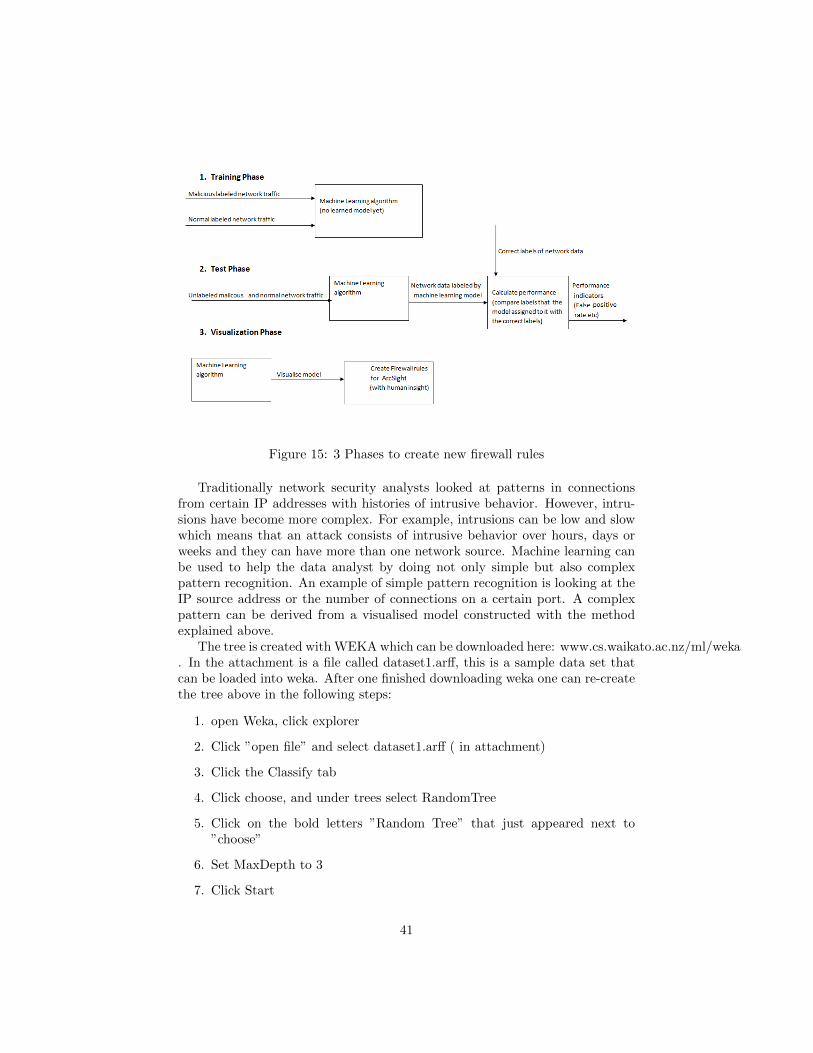
Figure 15: 3 Phases to create new firewall rules

Traditionally network security analysts looked at patterns in connectionsfrom certain IP addresses with histories of intrusive behavior. However, intru-sions have become more complex. For example, intrusions can be low and slowwhich means that an attack consists of intrusive behavior over hours, days orweeks and they can have more than one network source. Machine learning canbe used to help the data analyst by doing not only simple but also complexpattern recognition. An example of simple pattern recognition is looking at theIP source address or the number of connections on a certain port. A complexpattern can be derived from a visualised model constructed with the methodexplained above.

The tree is created with WEKA which can be downloaded here: www.cs.waikato.ac.nz/ml/weka. In the attachment is a file called dataset1.arff, this is a sample data set thatcan be loaded into weka. After one finished downloading weka one can re-createthe tree above in the following steps:

1. open Weka, click explorer

2. Click ”open file” and select dataset1.arff ( in attachment)

3. Click the Classify tab

4. Click choose, and under trees select RandomTree

5. Click on the bold letters ”Random Tree” that just appeared next to”choose”

6. Set MaxDepth to 3

7. Click Start

41

8. In the white area below where you just click start some text saying some-thing like ” trees.RandomTree” appeared, right click it and click visualisetree.

Network data is not a constant flow of data but consists of network packets.For each packet or for a group of packets one could determine whether thepacket or the group of packets is malicious or not. For simplicity in the examplewe determine per packet whether it is maliciouse or not. In the tree every nodeand leaf is numbered, and behind the number of the node and the ”:” is anumber indicating which byte is used by that node. The frequency of that bytedetermines what path through the tree should be followed. This is a very simpletree and this tree is not usable yet but gives an idea of the technique. Howeverthis decision tree did gave a recognition rate of 91.5% on the test set. If one hasa packet where the ”*” character occurs more than 0.5 times, the unit separatoroccurs less than 1.5 times, the NULL character occurs more than 128,5 timesand the destination port is smaller than the packet is classified as malicious.This can be seen by starting at the top of the tree, and following the decisionsdownward to the right leaf.

Using machine learning algorithms to detect intrusions has several advan-tages; it can detect zero-day malware because it can determine the statisticallikelihood that a program is malware based on previous examples.

D.3 The resulting firewall rules in ArcSight

From the model shown in 8 firewall rules can be created. In order to explainhow to create these rules, first examples of currently existing firewall rules inArcSight are shown below.

1. Rule Name: High Number of Connections Rule Desc: This rule detectsfirewall accept events for MSSQL, Terminal Services, and TFTP connec-tions (default destination ports: MSSQL=1433, Terminal Services=2289,TFTP=69). The rule triggers when ten events from the same device occurwithin 2 minutes. Rule Conditions:

event1 : ( Type = Base AND Category Behavior = /Access AND CategoryDevice Group = /Firewall AND Category Object = /Host/Application/ServiceAND Category Outcome = /Success AND ( Target Port = 1433 OR TargetPort = 3389 OR Target Port = 69 ) AND NotInActiveList(”Event-basedRule Exclusions”) )

2. Rule name: Possible Internal Network Sweep Rule Description: This ruledetects a single host trying to communicate with at least ten other hostson the same target port within the network, within a minute. This rule,combined with a spike in target port activity by the same host, resultsin the worm outbreak detected rule being triggered. Rule Conditions: 10matches in 1 minute of events. The 10 events that have different targetaddress but same target port and source address.

42

3. Data Monitor Name: Covert Channel DM Desc: This data monitor dis-plays event information indicating that there is a covert channel. Port 53is a well-known port for DNS, but DNS activity is generally UDP. Suchactivity can be correlated with covert channels. DM uses a filter that looksfor Destination Port = 53 and Transport Protocol = TCP.

If one looks at the visualised model one could use common sense and createmore of these rules. These rules can be much more advanced and complex.These complexer rules will lead to less false positives and less false negatives.This makes a better firewall. How good these rules are can be shown and provenwith statistics (phase 2 in 15). Without the machine learning certain complexrules will never be thought off because creating these rules is a very complexand difficult task.

D.4 Remarks

There are some remarks that need to be kept in mind when using this techniquein practice:

1. The data set containing normal and malicious packets on which machinelearning methods are applied and on which the model is trained is veryimportant. The machine learning method will learn to differentiate be-tween these malicious and normal packets. In this project malicious pack-ets are generated by performing attacks with Metasploit on a machinewith Metasploitable installed. Normal data is just dumps of capture ofnormal network traffic generated by browsing the Internet, downloadingsome files, reading mail and playing a video game online. So the modelwill learn to differentiate between these 2 different data sets.

2. The rules have to be derived from the visualised model. Human interpre-tation is needed in this process.

3. The model that is created should be tested, this is done by calculating falsepositive and false negative rates on a test set. This gives an indicationhow good the model is.

43

E Visualised experiments

E.0.1 Experiment 0

mal normclassified as mal 1497 379classified as norm 407 11037

Figure 16: Resulting tree of Experiment 0

E.0.2 Experiment 1


The tree of experiment 1 is omitted because it is too large.

E.0.3 Experiment 2


44

Figure 17: Resulting tree of experiment 2

E.0.4 experiment 3


The tree of experiment 3 is omitted because it is too large.

E.1 Experiment 4


Figure 18: Part 0 of the resulting tree of experiment 4

45



Confusion matrix:

46


E.1.1 experiment 6

Neural network:

Figure 21: Neural network of experiment 6

The confusion matrix:


E.2 Experiment 7

Confusion matrix:

47


Resulting Tree:

Figure 22: The resulting tree of experiment 7. The number after the P indicateswhich of the 8 packets, then comes the attribute

E.3 Experiment 8

Confusion matrix:


48

References

[C. Saeed] Chen Saeed, Thomas M., Abu-Nimeh. (2011) Lessons from stuxnet.Computer Volume:44 Issue: 4.

[R. Williams] Ronald D. Williams, Vinay M. Igure, Sean A. Laughter. (2006)Security issues in SCADA networks. Elsevier, Computers and security.

[M. Fossi] M. Fossi, D. Turner,T. Adams, J. Blackbird, S.Entwise, B.Graveland,D.McKinney, J. Mulcahy, C. Wueest, K Haley, E Johnson. (2009) Symantec,Internet Security Threat Report 2009. Symantec.

[A. Nicholson] A. Nicholson, S. Webber, S. Dyer, T. Patel, H. Janicke. (2012)SCADA security in the light of Cyber Warfare, Computers and security.

[Infosecurity] InfoSecurity-Magazine. (2009) MI5 hires teenage hackers in fightagainst cyberterrorism.

[V. Jyothsna] V. Jyothsna, V. Rama Prasad, K. Munivara Prasad. (2011)A Review of Anomaly based Intrusion Detection Systems. InternationalJournal of Computer Applications.

[O. Linda] Ondrej Linda, Todd Vollmer, Milos Manic. (2009) Neural networkBased Intrusion Detection System for Critical Infrastructures, InternationalJoint Conference on Neural networks.

[E. pleijsier] Erik Pleijsier. (2009) Towards Anomaly Detection in SCADANetworks using Connection Patterns, International Joint Conference onNeural networks.

[K. Rieck] Konrad Rieck, Philipp Trinius, Carsten Willems, Thorsten Holz.(2011) Automatic analysis of malware behavior using machine learning,Journal of computer security IOS Press.

[Kali] Offensive security. (2014) Kali Linux, Website: www.Kali.org, date ofdownload: 1 June 2014.

[Cyber arms] Cyberarms wordpress. (2013) worldwide map of internet con-nected SCADA Systems.

49

[Wireshark] Wireshark. (2014) Wireshark. Website: www.Wireshark.org, dateof download: 1 June 2014.

[Symantec] Symantec connect. (2010) KingView Heap Based Buffer OverflowVulnerability. Website: www.securityfocus.com/bid/45727/exploit, Date ofdownload: 1 june 2014.

[Metasploit] Rapid 7. (2014) Metasploit. Website: www.Metasploit.com, dateof download: 1 June 2014.

[Army magazine] Army magazine. (2014) Building Teams of Cyber Warriors.

[J. McHugh] J. McHugh. (2000) Testing intrusion detection systems: a critiqueof the 1998 and 1999 DARPA intrusion detection system evaluations asperformed by Lincoln Laboratory, ACM Transactions on Information andSystem Security.

[J. Jonathan] J. Jonathan, Davisa, K. Andrew, Clark. (2011) Data Preprocess-ing for Anomaly Based Network Intrusion Detection: A Review, Compuerand Security.

[KDDcup] Knowledge discovery and datamining. (1999) KDD Cup 1999:Computer network intrusion detection. Website: www.sigkdd.org/kdd-cup-1999-computer-network-intrusion-detection, date of download: 1 May 2014.

[P. Ahmed] P. Ahmed, Amrita. (2013) A Hybrid-Based Feature SelectionApproach for IDS, NetCom 2013

[S. Kumar] A. Arya, S. Kumar. (2014) Information theoretic feature extractionto reduce dimensionality of Genetic Network Programming based intrusiondetection model. ICIT 2014.

[U. Subramanian] U. Subramanian, Hang See Ong. (2014)Analysis of the Effectof Clustering the Training Data in Naive Bayes Classifier for AnomalyNetwork Intrusion Detection. Journal of Advances in Computer Networks.

[DARPA] MIT. (1999) DARPA Intrusion Detection Data Sets. Website:www.ll.mit.edu/mission/communications/cyber/CSTcorpora/ideval/data,date of download: 1 may 2014.

50

[K. Rajitha] K. Rajitha, Dr.D. Vijaya Lakshmi, R. Udaya, Sreekanth. (2014)Mining Technique For DARPA 99 Intrusion Detection Data Set. Interna-tional Conference on Computer and Communication Technologies 2K14.

[R. Perdisci] Roberto Perdisci. (2008) McPAD : A Multiple Classier System forAccurate Payload-based Anomaly Detection. Elsevier Science.

[LookupTables] lookup tables. Website: www.lookupTables.com, date ofdownload: 1 may 2014.

[Rapid7] Metasploitable 2.0. Website: www.information.rapid7.com/Metasploitable-download.html, date of download: 1 june 2014.

[vulns] Vulnerabilities in Metasploitable 2.0. Website:www.hackertarget.com/sample/nexpose-Metasploitable-test.pdf, date ofdownload: 1 may 2014.

[tcpDump] tcpdump. Website: www.tcpdump.org/manpages/tcpdump.1.html,date of download: 1 may 2014.

[Winpcap] WinPcap a pcap library for JAVA. Website: www.winpcap.org/,date of download: 15 may 2014.

[I. S. Dhillon] ] I. S. Dhillon, S. Mallela, and R. Kumar. (2003) A divisiveinformation-theoreticfeature clustering algorithm for text classifica-tion, Journal of MachineLearning Research, 3:12651287, 2003. Website:www.dl.acm.org/citation.cfm?id=944973, date of download: 15 june 2014.

[S. Warren] S. Warren, McCulloch and Walter Pitts. (1943) A logical calculusof the ideas immanent in nervous activity, Bulletin of mathematicalbiophysics 5.

[C. Mihaescu] Dr. Ing. Cristian Mihaescu. Flat Clustering K-means algorithm.Website: www-users.cs.umn.edu/ han/dmclass/cluster survey 10 02 00.pdf,date of download: 1 may 2014.

[M. Eldracher] M. Eldracher. (1992) Classification of Non-Linear-SeparableReal-World-Problems Using deltaRule, Perceptrons, and TopologicallyDistributed Encoding. Applied Computing: Technological Challenges of the1990s.

51

[K. Hornik] Kur Hornik. (1989) Multilayer feedforward networks are universalapproximators, Neural networks Vol. 2.

[M. W. Gardner] M. W. Gardner, S. R. Dorling. (1998) Artificial neuralnetworks (the multilayer perceptron) - A review of applications in theatmospheric sciences, Atmospheric environment Vol.32 Elsevier.

[F. Piekniewski] F. Piekniewski and Leszek Rybicki. (2004) Visualizing andAnalyzing Multidimensional Output from MLP Networks via BarycentricProjections, Departament of Mathematics and Computer Science.

[M. Tom] M. Tom. Mitchell. (1997) Machine Learning, McGraw-Hill Sci-ence/Engineering/Math.

[A. Blumer] A. Blumer. (1987) Occam’s Razor, Information processing lettersvolume 24.

[G. Lovet] Guillaume Lovet. (2006) Dirty Money on the Wires: The BusinessModels of Cyber Criminals. Virus Bulletin Conference 2006.

[M. Clement] M. Clement. (2008) The Cost Impact of Spam Filters: Mea-suring the Effect of Information System Technologies in Organizations.University of Hamburg Institute for Marketing and Media. Website:www.d-nb.info/1006920315/34, date of download: 15 april 2014.

[C. Kanich] C. Kanich, C. Kreibich, K. Levchenko, B. Enright, G. M. Voelker,V. Paxson, and S. Savage. Spamalytics: An empirical analysis of spam mar-keting conversion. In Proceedings of the 15th ACM Conference on Computerand Communications Security.

[M. Fossi] M. Fossi, D. Turner, T. Adams, J. Blackbird, S.Entwise,B.Graveland, D.McKinney, J. Mulcahy, C. Wueest. , K Haley, E Johnson.(2010) Symantec, Internet Security Threat Report 2009. Methodology, 2008Symantec.

[S. Mukkamala] S. Mukkamala. (2002) Intrusion detection using neural net-works and Support Vector machines, New Mexico Institute of Mining andTechnology.

[L. Breiman] Leo Breiman. (2001) Random Forests, Machine learning Springer.

52

[M. Eeten] M. van Eeten, J.M. Bauer, S. Tabatabaie. (2009) Damages frominternet security incidents. A framework and toolkit for assessing theeconomic costs of security breaches. TU Delft.

[B. Cashell] B. Cashell, William D. Jackson, M. Jickling, and B. Webel. (2004)The Economic Impact of Cyber-Attacks, Government and Finance Division.

[McAfee] McAfee, center for strategic and international studies. (2013) TheImpact of Cybercrime and cyber espionage.

[T. Dietterich] Thomas G. Dietterich. (2000) An Experimental Comparison ofThree Methods for Constructing Ensembles of Decision Trees: Bagging,Boosting, and Randomization, Machine Learning, springer.

[O. Maron] Oded Maron, Tomas Lozano-Perez. (1998) A Framework forMultiple-Instance Learning, AI Lab , M.I.T.Website: www.lis.csail.mit.edu/pubs/tlp/maron98framework.pdf, date ofdownload: 15 june 2014.

[M.v.j.] Ministerie van Veiligheid en Justitie. (2010) Nationaal TrendrapportCybercrime en Digitale Veiligheid.

[T. Jaochims] Thorsten Jaochims, Dortmunt. (1997) Text categorization withsupport vector machines: learning with many relevant features, Universityof Dortmund.

[E. Mizutani] Eiji Mizutani and Stuart E. Dreyfus. (2001) On complexityanalysis of supervised MLP-learning for algorithmic comparisons, IEEE.

[I. Weon] Ill-Young Weon, Doo-Heon Song, Sung-Bum Ko, Chang-Hoon Lee.(2005) Multiple Instance Learning Problem Approach Model to AnomalyNetwork Intrusion Detection, International Journal of Information Process-ing Systems Vol.1, No.1.

[A. Simmonds] Andrew Simmonds, Peter Sandilands, Louis van Ekert. (2004)Lecture Notes in Computer Science Volume 3285, 2004.

53

creating firewall rules with machine learning techniques

Documents