coupled mathematical programming and cge modelling … · coupled mathematical programming and cge...

Coupled mathematical programming and CGE modelling for drought policy assessment

C. D. Pérez-Blanco, FEEM & CMCC

Mathematical programming and CGE modelling

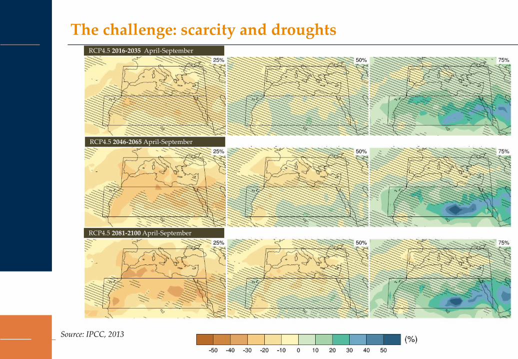
The challenge: scarcity and droughts

Source: IPCC, 2013

RCP4.5 2016-2035 April-September




The challenge: scarcity and droughts

> Water crises are perceived as the most relevant global risk in terms of impact> Irrigation represents 70% of total water withdrawals worldwide> CC will reduce supply. Demand for crop irrigation is expected to increase by more than 40% up to 2080

> Absolute scarcity is a reality already

> How can we adapt? What will be the repercussions?


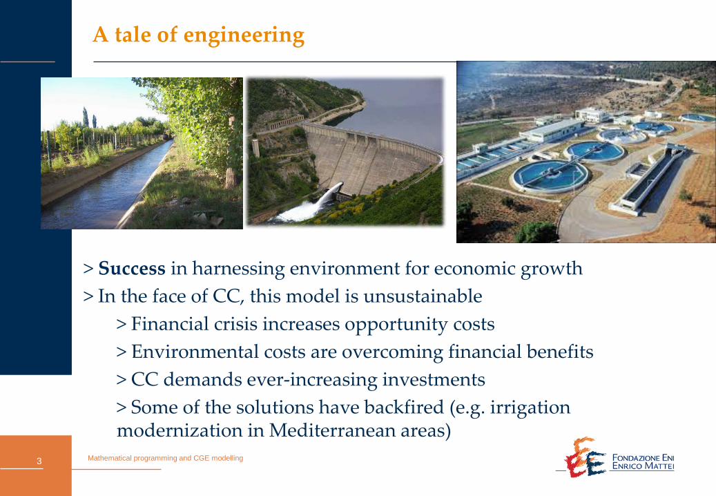
A tale of engineering

> Success in harnessing environment for economic growth> In the face of CC, this model is unsustainable

> Financial crisis increases opportunity costs> Environmental costs are overcoming financial benefits> CC demands ever-increasing investments> Some of the solutions have backfired (e.g. irrigation modernization in Mediterranean areas)

3


Managing demand

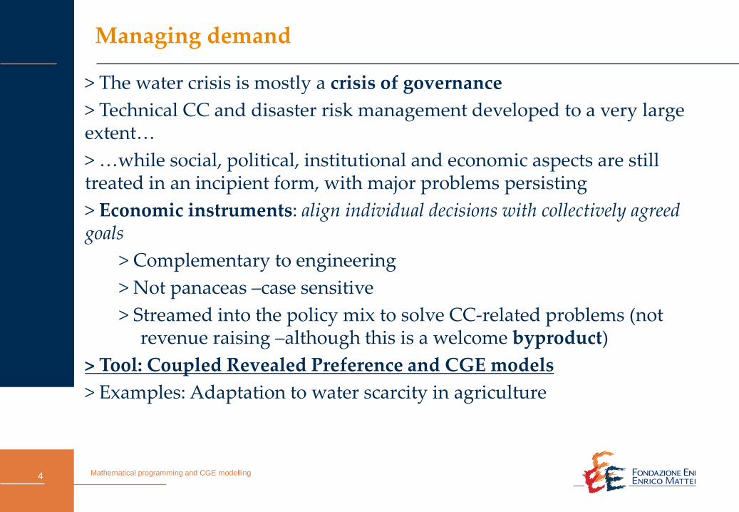
> The water crisis is mostly a crisis of governance> Technical CC and disaster risk management developed to a very large extent…> …while social, political, institutional and economic aspects are still treated in an incipient form, with major problems persisting> Economic instruments: align individual decisions with collectively agreed goals

> Complementary to engineering> Not panaceas –case sensitive> Streamed into the policy mix to solve CC-related problems (not

revenue raising –although this is a welcome byproduct)> Tool: Coupled Revealed Preference and CGE models> Examples: Adaptation to water scarcity in agriculture

4

Chapter 1: Coupling with droughts in the Regione Emilia Romagna (Italy)


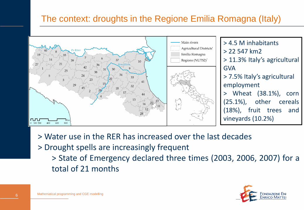
The context: droughts in the Regione Emilia Romagna (Italy)

> Water use in the RER has increased over the last decades> Drought spells are increasingly frequent

> State of Emergency declared three times (2003, 2006, 2007) for atotal of 21 months

> 4.5 M inhabitants> 22 547 km2> 11.3% Italy’s agriculturalGVA> 7.5% Italy’s agriculturalemployment> Wheat (38.1%), corn(25.1%), other cereals(18%), fruit trees andvineyards (10.2%)

6


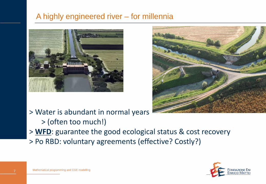
A highly engineered river – for millennia

> Water is abundant in normal years > (often too much!)

> WFD: guarantee the good ecological status & cost recovery> Po RBD: voluntary agreements (effective? Costly?)

7


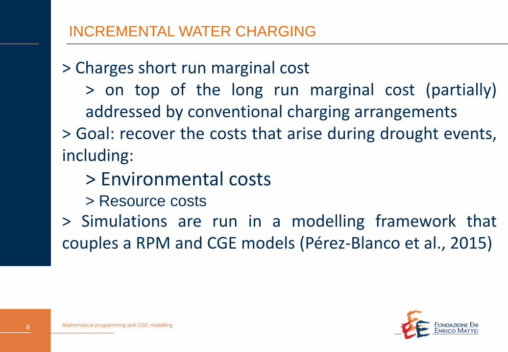
INCREMENTAL WATER CHARGING

> Charges short run marginal cost> on top of the long run marginal cost (partially)addressed by conventional charging arrangements

> Goal: recover the costs that arise during drought events,including:

> Environmental costs> Resource costs

> Simulations are run in a modelling framework thatcouples a RPM and CGE models (Pérez-Blanco et al., 2015)

8


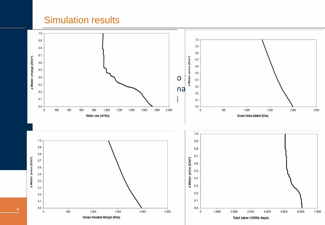
Simulation results

> Incremental charges from 0 to 100 Eurocents/m3 are tested> Water use, gross variable margin, employment generation andgross value added are assessed

9


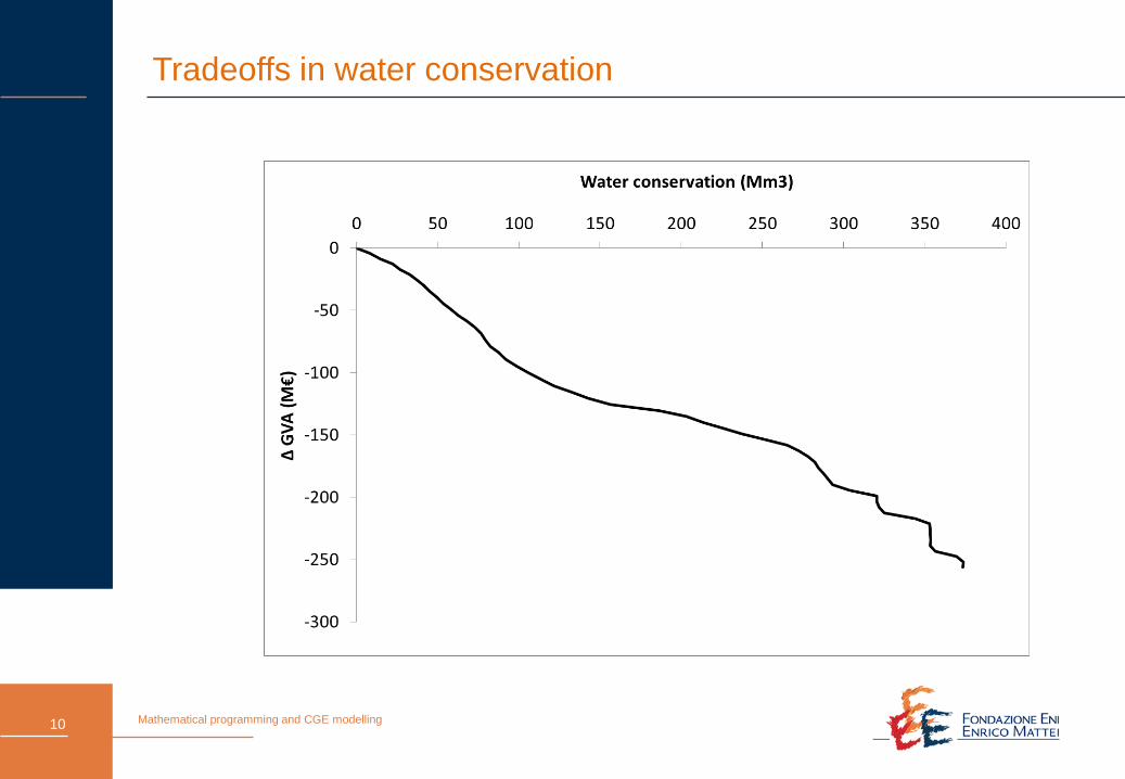
Tradeoffs in water conservation

10


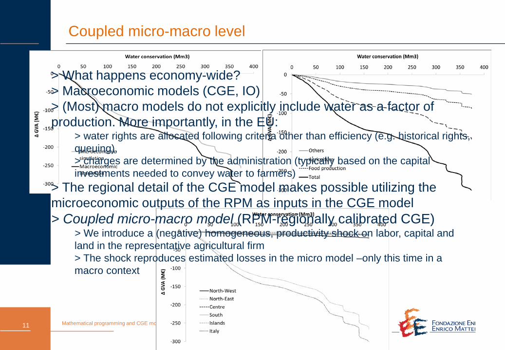
Coupled micro-macro level

> What happens economy-wide?> Macroeconomic models (CGE, IO)> (Most) macro models do not explicitly include water as a factor of production. More importantly, in the EU:

> water rights are allocated following criteria other than efficiency (e.g. historical rights, queuing), > charges are determined by the administration (typically based on the capital investments needed to convey water to farmers)

> The regional detail of the CGE model makes possible utilizing the microeconomic outputs of the RPM as inputs in the CGE model > Coupled micro-macro model (RPM-regionally calibrated CGE)

> We introduce a (negative) homogeneous, productivity shock on labor, capital and land in the representative agricultural firm> The shock reproduces estimated losses in the micro model –only this time in a macro context

11


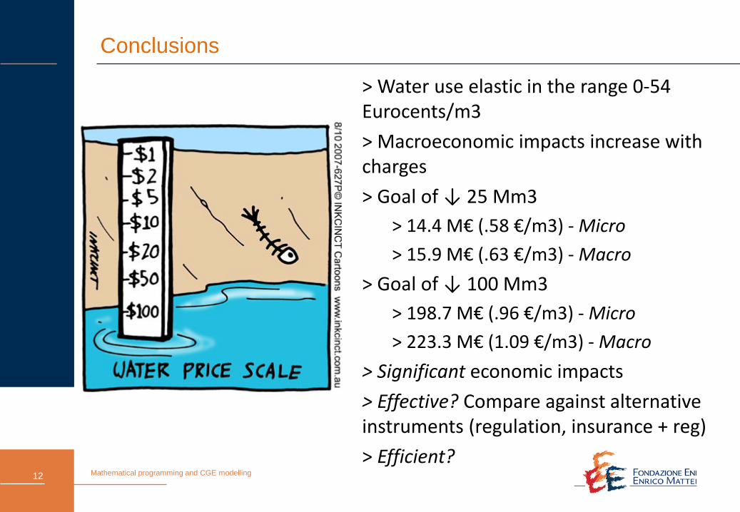
Conclusions

> Water use elastic in the range 0-54 Eurocents/m3> Macroeconomic impacts increase with charges> Goal of ↓ 25 Mm3

> 14.4 M€ (.58 €/m3) - Micro> 15.9 M€ (.63 €/m3) - Macro

> Goal of ↓ 100 Mm3> 198.7 M€ (.96 €/m3) - Micro> 223.3 M€ (1.09 €/m3) - Macro

> Significant economic impacts> Effective? Compare against alternative instruments (regulation, insurance + reg)> Efficient?

12

Chapter 2: The absolute water scarce Segura River Basin (Spain)


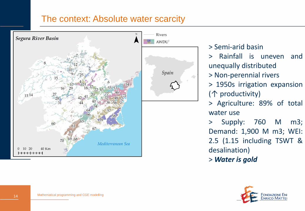
> Semi-arid basin> Rainfall is uneven andunequally distributed> Non-perennial rivers> 1950s irrigation expansion(↑ productivity)> Agriculture: 89% of totalwater use> Supply: 760 M m3;Demand: 1,900 M m3; WEI:2.5 (1.15 including TSWT &desalination)> Water is gold

The context: Absolute water scarcity

14


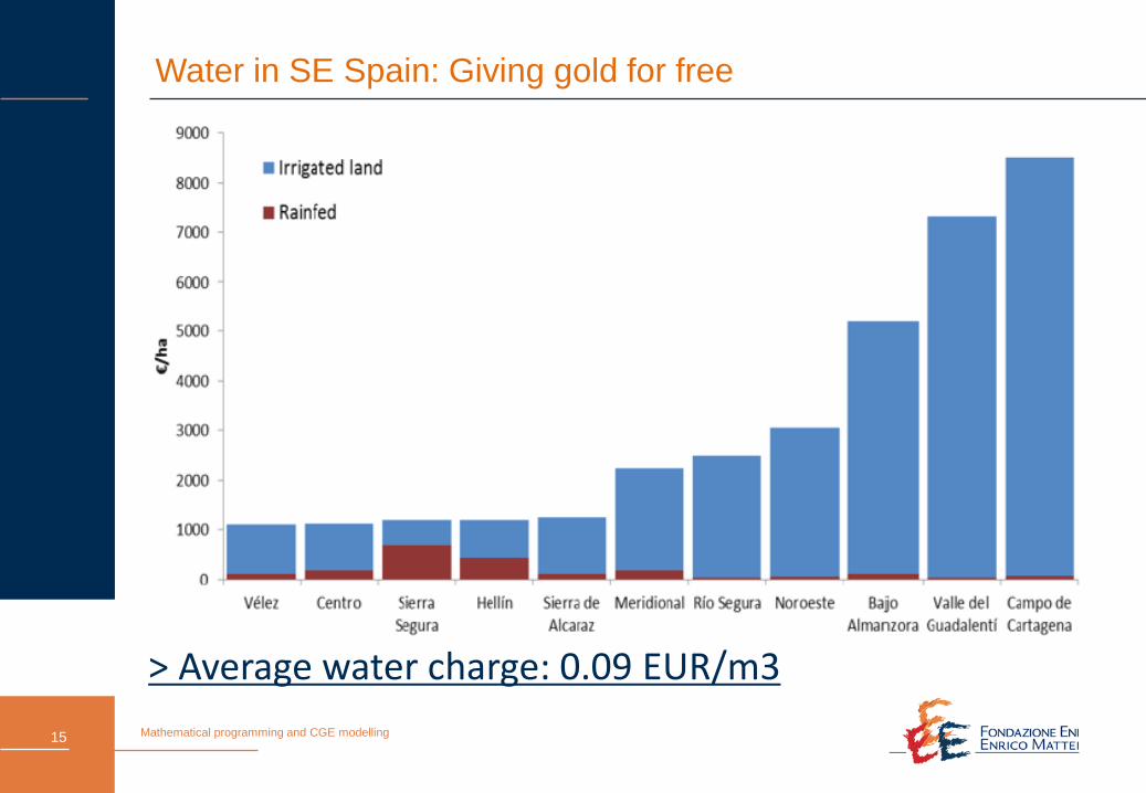
Water in SE Spain: Giving gold for free

> Average water charge: 0.09 EUR/m315


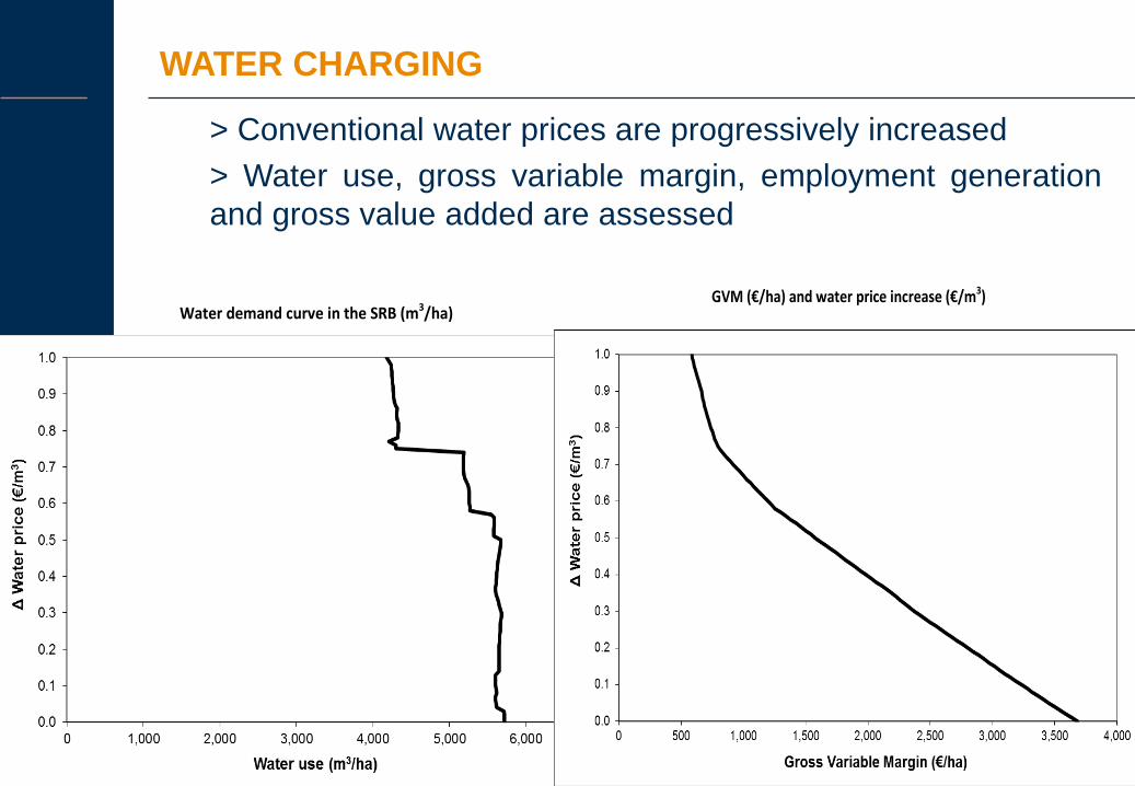
WATER CHARGING

> Conventional water prices are progressively increased> Water use, gross variable margin, employment generationand gross value added are assessed

Water demand curve in the SRB (m3/ha)

GVM (€/ha) and water price increase (€/m3)


Conclusions

> EU belief: ↑ water Prices => ↓ Water use (EC, 2000, 2012)> This is at best debatable (Cornish et al., 2004; Perry, 2005; Steenbergen et al., 2007…)> ↑ P may ↓ GVM, marginal impact on W

>What about the SRB?> ↑ P improve low CR ratios (54-81%)> But are insufficient to ↓ W

> Until unrealistic ↑ P over 600%

> What can be done?

17


WATER BUYBACK

> De iure, RBAs are entitled to limit/revoke water concessions thatharm the environment, without compensation> De facto, concessions are renewed automatically

> Transaction costs> Negative economic impact on rural areas

> Water buyback aims at:> restoring environmental flows;> compensating farmers (& overcome resistance); and> compensating other possible negative feedbacks

> Since 2006 government agencies can use exchange centers to buywater concessions> We estimate a benchmark to inform and assess water purchasetenders (compensating variation)

18


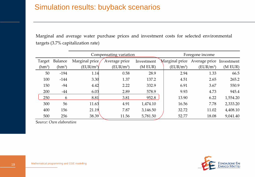
Simulation results: buyback scenarios

Marginal and average water purchase prices and investment costs for selected environmental targets (3.7% capitalization rate)

Compensating variation Foregone income Target (hm3)

Balance (hm3)

Marginal price (EUR/m3)

Average price (EUR/m3)

Investment (M EUR)

Marginal price (EUR/m3)

Average price (EUR/m3)

Investment (M EUR)

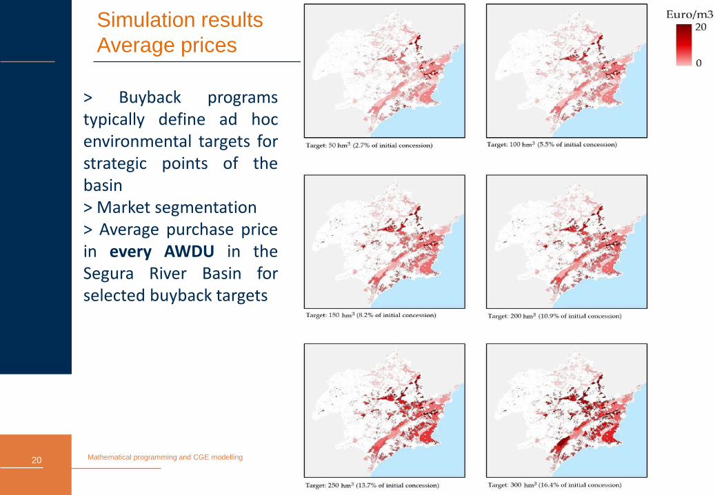
50 -194 1.14 0.58 28.9 2.94 1.33 66.5 100 -144 3.30 1.37 137.2 4.51 2.65 265.2 150 -94 4.42 2.22 332.9 6.91 3.67 550.9 200 -44 6.03 2.89 578.9 9.93 4.73 945.4 250 6 8.81 3.81 952.8 13.90 6.22 1,554.20 300 56 11.63 4.91 1,474.10 16.56 7.78 2,333.20 400 156 21.19 7.87 3,146.50 32.72 11.02 4,408.10 500 256 38.39 11.56 5,781.50 52.77 18.08 9,041.40

Source: Own elaboration

19


Simulation resultsAverage prices

> Buyback programstypically define ad hocenvironmental targets forstrategic points of thebasin> Market segmentation> Average purchase pricein every AWDU in theSegura River Basin forselected buyback targets

20


Conclusions> Water buyback can help restore the balance

> Average price about 3.8 EUR/m3

> A few caveats:

> Informal abstractions: track and ban, do not empower (not again!)> Use water bought for environmental purposes

> not to maintain allotments during droughts (define ecologicalflows)

> Define priority areas for buyback (downstream vs upstream)> This is but a policy option –others may exist

> Charges> Insurance> etc.

> Explore complementarities, sequencing> Transaction costs are the key

21

Chapter 3: No silver bullets…


Some remarks

> Economic instruments complement supply policies> Both are preconditions for a successful policy mix

> Putting all together –be aware of:> Institutional setup – the peril of transaction costs> Policy mix> Sequencing and spillovers

> And remember: there are no silver bullets> You better learn from other experiences… > …but it is the context what ultimately determines the solution

23

Thanks for your attention

This research is part of a project that has received funding fromthe European Union’s Horizon 2020 research and innovationprogramme under the Marie Skłodowska-Curie grant agreementNo 660608.

http://wateragora.eu/24

http://wateragora.eu/

Annex

25


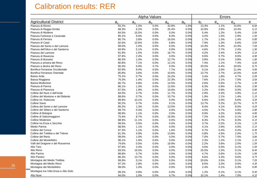
Calibration results: RERAlpha Values Errors

Agricultural District a1 a2 a3 a4 a5 ef ea ed ePianura di Rimini 55.2% 1.0% 0.0% 42.8% 1.0% 13.3% 1.1% 14.6% 6.6%Pianura di Reggio Emilia 68.3% 6.2% 0.0% 25.4% 0.0% 10.9% 2.6% 10.4% 5.1%Pianura di Modena 84.5% 15.5% 0.0% 0.0% 0.0% 5.4% 1.2% 5.4% 2.6%Pianura Forlivese e Cesenate 85.1% 6.6% 0.0% 8.3% 0.0% 3.2% 1.5% 2.9% 1.5%Pianura di Ferrara 80.7% 2.8% 0.0% 16.5% 0.0% 1.7% 1.3% 1.4% 0.8%Pianura di Carpi 82.6% 10.6% 0.0% 6.8% 0.0% 7.9% 1.3% 6.6% 3.5%Pianura del Senio e del Lamone 99.0% 1.0% 0.0% 0.0% 0.0% 14.3% 5.4% 14.3% 7.0%Pianura dell’Idice e del Santerno 94.9% 5.1% 0.0% 0.0% 0.0% 4.6% 2.7% 2.4% 1.9%Pianura del Lamone 81.9% 1.5% 0.0% 16.7% 0.0% 4.2% 2.4% 4.3% 2.1%Pianura di Ravenna 97.6% 2.4% 0.0% 0.0% 0.0% 9.6% 5.7% 9.6% 4.9%Pianura di Busseto 86.3% 1.0% 0.0% 12.7% 0.0% 3.8% 0.1% 3.8% 1.8%Pianura a sinistra del Reno 80.8% 7.1% 0.0% 12.1% 0.0% 7.4% 1.1% 7.4% 3.5%Pianura a destra del Reno 90.4% 5.9% 3.7% 0.0% 0.0% 20.5% 6.4% 19.5% 9.7%Bonifica Ferrarese Occidentale 82.9% 9.4% 0.0% 7.7% 0.0% 9.1% 2.0% 11.4% 4.9%Bonifica Ferrarese Orientale 85.8% 3.6% 0.0% 10.6% 0.0% 13.7% 2.7% 14.0% 6.6%Basso Arda 75.1% 0.7% 0.0% 24.2% 0.0% 3.4% 1.8% 4.7% 2.0%Bassa Reggiana 76.3% 1.4% 0.0% 22.3% 0.0% 7.6% 2.1% 7.0% 3.5%Bassa Modenese 80.7% 4.8% 0.0% 14.5% 0.0% 2.6% 0.5% 2.7% 1.3%Pianura di Parma 86.1% 1.3% 0.0% 12.6% 0.0% 6.3% 0.9% 6.0% 2.9%Pianura di Piacenza 87.5% 1.9% 0.0% 10.6% 0.0% 2.2% 0.9% 0.0% 0.8%Colline del Nure e dell’Arda 84.5% 3.7% 0.0% 11.7% 0.0% 2.9% 4.3% 3.9% 2.1%Colline del Montone e del Bidente 88.6% 0.7% 0.0% 10.7% 0.0% 1.9% 2.1% 1.4% 1.1%Colline int. Rubicone 89.9% 10.1% 0.0% 0.0% 0.0% 6.6% 2.0% 6.6% 3.2%Colline Savio 90.2% 0.7% 0.0% 9.1% 0.0% 13.7% 5.2% 13.7% 6.7%Collina del Senio e del Lamone 85.2% 1.3% 0.0% 13.5% 0.0% 8.4% 4.1% 8.5% 4.2%Colline del Sillaro e del Santerno 99.7% 0.3% 0.0% 0.0% 0.0% 4.5% 5.7% 4.5% 2.8%Colline di Bologna 98.9% 1.1% 0.0% 0.0% 0.0% 9.9% 4.2% 9.9% 4.9%Colline di Salsomaggiore 75.4% 8.7% 0.0% 15.9% 0.0% 7.2% 0.3% 0.1% 2.4%Colline Modenesi 88.9% 11.1% 0.0% 0.0% 0.0% 8.3% 3.7% 8.3% 4.1%Colline tra Enza e Secchia 99.5% 0.5% 0.0% 0.0% 0.0% 3.7% 0.2% 0.1% 1.2%Medio Parma 98.9% 1.1% 0.0% 0.0% 0.0% 4.1% 2.9% 4.0% 2.1%Colline del Conca 97.3% 1.1% 0.0% 1.6% 0.0% 0.7% 0.4% 0.4% 0.3%Colline del Trebbia e del Tidone 81.3% 4.9% 0.0% 13.8% 0.0% 0.8% 4.5% 2.0% 1.7%Colline del Reno 99.0% 1.0% 0.0% 0.0% 0.0% 7.0% 5.7% 7.0% 3.8%Colline del Montefeltro 98.1% 1.9% 0.0% 0.0% 0.0% 2.3% 1.2% 2.1% 1.1%Valli del Dragone e del Rossenna 79.6% 0.5% 0.0% 19.9% 0.0% 2.2% 3.6% 2.0% 1.5%Alto Taro 97.6% 2.4% 0.0% 0.0% 0.0% 4.6% 0.5% 0.1% 1.5%Alto Reno 83.5% 16.5% 0.0% 0.0% 0.0% 25.0% 2.3% 0.1% 8.4%Alto Parma 98.8% 0.7% 0.0% 0.5% 0.0% 4.7% 0.6% 0.1% 1.6%Alto Panaro 86.3% 13.7% 0.0% 0.0% 0.0% 9.6% 3.3% 9.6% 4.7%Montagna del Medio Trebbia 99.9% 0.1% 0.0% 0.0% 0.0% 20.6% 3.5% 0.1% 7.0%Montagna del Medio Reno 97.2% 2.8% 0.0% 0.0% 0.0% 8.5% 3.3% 9.0% 4.3%Montagna del Montefeltro 99.0% 1.0% 0.0% 0.0% 0.0% 2.4% 0.1% 0.3% 0.8%Montagna tra l’Alto Enza e Alto Dolo 99.2% 0.8% 0.0% 0.0% 0.0% 1.2% 0.1% 0.1% 0.4%Alto Nure 94.0% 1.0% 0.0% 4.7% 0.0% 10.1% 1.4% 7.0% 4.1%

26


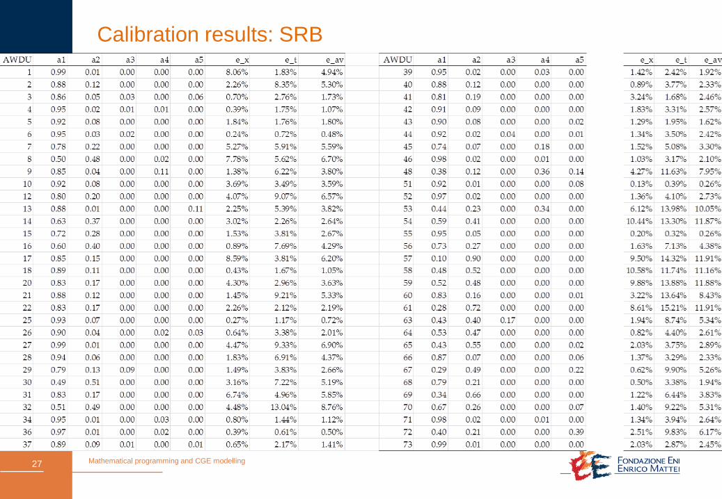
Calibration results: SRB

27


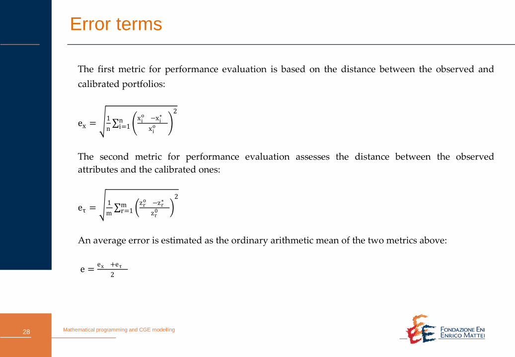
Error terms

The first metric for performance evaluation is based on the distance between the observed and calibrated portfolios:

ex = �1n∑ �xi

o −xi∗

xio �

2ni=1

The second metric for performance evaluation assesses the distance between the observed attributes and the calibrated ones:

eτ = �1m∑ �zr

o −zr∗

zr0 �

2mr=1

An average error is estimated as the ordinary arithmetic mean of the two metrics above:

e = ex +eτ2

28

coupled mathematical programming and cge modelling … · coupled mathematical programming and cge...

Documents