Counting spanning trees

Question Given a graph G, how many spanning trees does G have?

⌧ (G) = number of distinct spanning trees of G

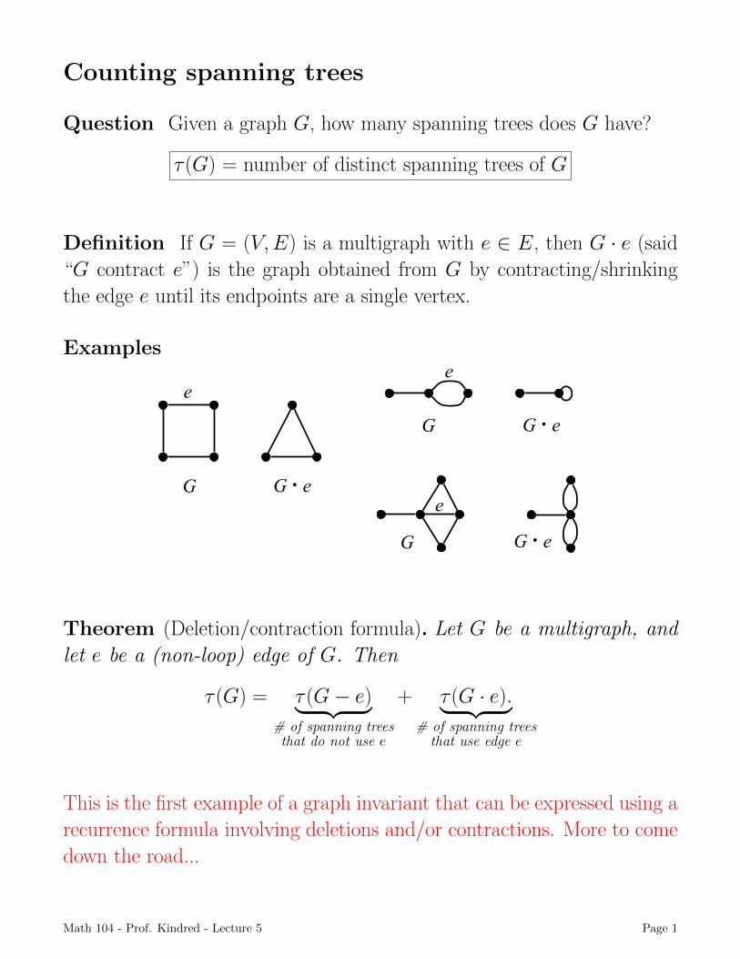
Definition If G = (V,E) is a multigraph with e 2 E, then G · e (said

“G contract e”) is the graph obtained from G by contracting/shrinking

the edge e until its endpoints are a single vertex.

Examples

G

e

G ･ e

G

e

G ･ e

e

G G ･ e

Theorem (Deletion/contraction formula). Let G be a multigraph, and

let e be a (non-loop) edge of G. Then

⌧ (G) = ⌧ (G� e)| {z }# of spanning trees

that do not use e

+ ⌧ (G · e).| {z }# of spanning trees

that use edge e

This is the first example of a graph invariant that can be expressed using a

recurrence formula involving deletions and/or contractions. More to come

down the road...

Math 104 - Prof. Kindred - Lecture 5 Page 1

Comment on proof Need to show a one-to-one correspondence between

spanning trees of G that include e and spanning trees of G · e.spanning tree T of G that uses e ! T · e, a spanning tree of G · e

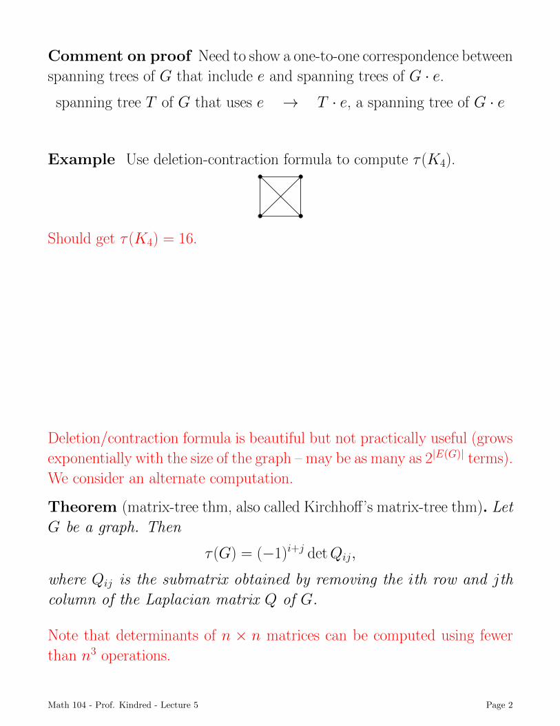
Example Use deletion-contraction formula to compute ⌧ (K4).

Should get ⌧ (K4) = 16.

Deletion/contraction formula is beautiful but not practically useful (grows

exponentially with the size of the graph – may be as many as 2|E(G)| terms).

We consider an alternate computation.

Theorem (matrix-tree thm, also called Kirchho↵’s matrix-tree thm). Let

G be a graph. Then

⌧ (G) = (�1)i+j detQij,

where Qij is the submatrix obtained by removing the ith row and jth

column of the Laplacian matrix Q of G.

Note that determinants of n ⇥ n matrices can be computed using fewer

than n3 operations.

Math 104 - Prof. Kindred - Lecture 5 Page 2

Remark Alternatively, we can express the matrix-tree theorem as

⌧ (G) =1

n�1�2 · · ·�n�1

where �1, . . . ,�n�1 are n� 1 largest eigenvalues of Laplacian matrix of G.

This calculation was first devised by Gustav Kircho↵ in 1847 as a way of

obtaining values of current flow in electrical networks. (Matrices were first

emerging as a powerful mathematical tool about the same time.)

Theorem (Cayley1, 1889).

⌧ (Kn) = nn�2.

Proof. We prove as a special case of the matrix-tree theorem. Let A be

the adjacency matrix of Kn. Then

A =

2

640

.

.

.

0

3

751

10

0= J � I ,

where J is the n⇥ n matrix of all ones and I is the identity matrix. The

Laplacian matrix, Q, of Kn is

Q = D�A = (n� 1)I� (J� I) = nI�J =

2

666664

n � 1

n � 1

.

.

.

n � 1

n � 1

3

777775-1

-1

Note that the vector of all ones is an eigenvector of Q for � = 0, and2

664

1

�1

0

0

.

.

.

0

3

775 ,

2

664

0

1

�1

0

.

.

.

0

3

775 , · · · ,

2

664

0

0

.

.

.

0

1

�1

3

775 ,

1Cayley was interested in representing hydrocarbons by graphs, and in particular, by trees.

Math 104 - Prof. Kindred - Lecture 5 Page 3

are linearly independent eigenvectors for � = n. Thus,

⌧ (Kn) =1

n(nn�1) = nn�2.

⌅

Remark Cayley’s formula may also be viewed as the number of possible

trees on the vertex set [n] = {1, 2, . . . , n}, i.e., the # of labelled trees on

n vtcs.

We have now answered the following question:

Of the 2(n2

) simple graphs with vertex set {1, 2, . . . , n}, how many

are trees?

? Book gives a proof of Cayley’s theorem using Prufer codes (unique se-

quence of length n� 2 assigned to a tree on n vtcs).

Math 104 - Prof. Kindred - Lecture 5 Page 4

Minimum spanning trees

Definition A weighted graph is a graph G = (V,E) with weight func-

tion w : E ! R.

Weights usually represent costs, distances, etc.

Minimum spanning tree problem – given a weighted con-

nected graph, find a spanning tree T with minimum

weight

w(T ) =X

e2E(T )

w(e).

We may see later that one application of minimum spanning trees is for an

approximation algorithm for the Traveling Salesman Problem (TSP).

Brute-force: construct all possible spanning trees and find one with mini-

mum weight.

Greedy algorithm =) any algorithm that makes a locally optimal

choice at each step with the aim of finding the

global optimum

(Downfall – can get locked into certain choices too early which prevent them

from finding the best overall solution later.)

Kruskal’s algorithm (greedy algorithm)

1. Order edges e1, . . . , em so that w(ei) w(ej) for any i < j.

2. T ;.

3. For k = 1 to m, if T + ek is acyclic, then T T + ek.

4. Output T .

Math 104 - Prof. Kindred - Lecture 5 Page 5

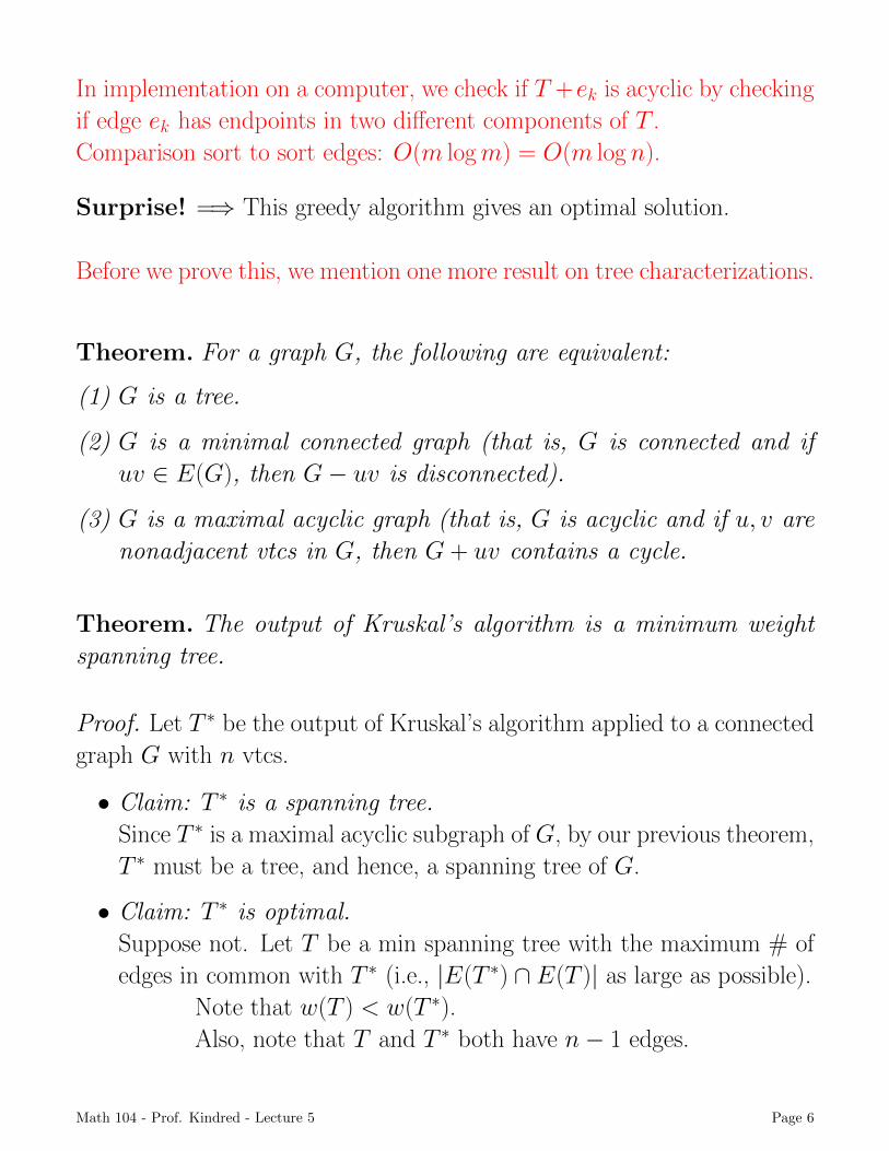
In implementation on a computer, we check if T +ek is acyclic by checking

if edge ek has endpoints in two di↵erent components of T .

Comparison sort to sort edges: O(m logm) = O(m log n).

Surprise! =) This greedy algorithm gives an optimal solution.

Before we prove this, we mention one more result on tree characterizations.

Theorem. For a graph G, the following are equivalent:

(1) G is a tree.

(2) G is a minimal connected graph (that is, G is connected and if

uv 2 E(G), then G� uv is disconnected).

(3) G is a maximal acyclic graph (that is, G is acyclic and if u, v are

nonadjacent vtcs in G, then G + uv contains a cycle.

Theorem. The output of Kruskal’s algorithm is a minimum weight

spanning tree.

Proof. Let T ⇤ be the output of Kruskal’s algorithm applied to a connected

graph G with n vtcs.

• Claim: T ⇤ is a spanning tree.

Since T ⇤ is a maximal acyclic subgraph of G, by our previous theorem,

T ⇤ must be a tree, and hence, a spanning tree of G.

• Claim: T ⇤ is optimal.

Suppose not. Let T be a min spanning tree with the maximum # of

edges in common with T ⇤ (i.e., |E(T ⇤) \ E(T )| as large as possible).Note that w(T ) < w(T ⇤).

Also, note that T and T ⇤ both have n� 1 edges.

Math 104 - Prof. Kindred - Lecture 5 Page 6

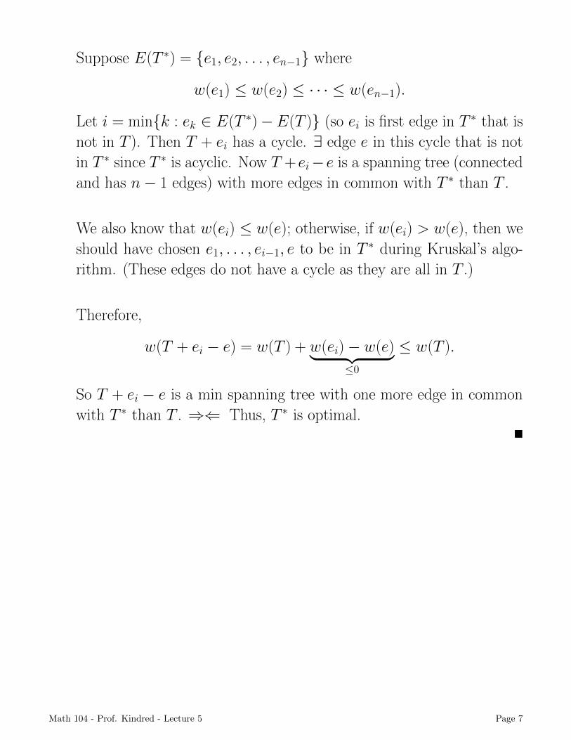
Suppose E(T ⇤) = {e1, e2, . . . , en�1} where

w(e1) w(e2) · · · w(en�1).

Let i = min{k : ek 2 E(T ⇤)�E(T )} (so ei is first edge in T ⇤ that is

not in T ). Then T + ei has a cycle. 9 edge e in this cycle that is not

in T ⇤ since T ⇤ is acyclic. Now T +ei�e is a spanning tree (connected

and has n� 1 edges) with more edges in common with T ⇤ than T .

We also know that w(ei) w(e); otherwise, if w(ei) > w(e), then we

should have chosen e1, . . . , ei�1, e to be in T ⇤ during Kruskal’s algo-

rithm. (These edges do not have a cycle as they are all in T .)

Therefore,

w(T + ei � e) = w(T ) + w(ei)� w(e)| {z }0

w(T ).

So T + ei � e is a min spanning tree with one more edge in common

with T ⇤ than T . )( Thus, T ⇤ is optimal.⌅

Math 104 - Prof. Kindred - Lecture 5 Page 7

Spanning treesMath 104, Graph TheoryTuesday, February 5, 2013

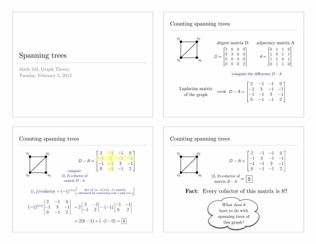
Counting spanning trees

v1 v2

v3 v4D =

�

⇧⇧⇤

2 0 0 00 3 0 00 0 3 00 0 0 2

⇥

⌃⌃⌅

degree matrix D adjacency matrix A

A =

�

⇧⇧⇤

0 1 1 01 0 1 11 1 0 10 1 1 0

⇥

⌃⌃⌅

D � A =

�

⇧⇧⇤

2 �1 �1 0�1 3 �1 �1�1 �1 3 �10 �1 �1 2

⇥

⌃⌃⌅=)Laplacian matrix of the graph

compute the di!erence D - A

Counting spanning trees

D � A =

�

⇧⇧⇤

2 �1 �1 0�1 3 �1 �1�1 �1 3 �10 �1 �1 2

⇥

⌃⌃⌅

compute (2, 2)-cofactor of

matrix D - A

(�1)2+2������

2 �1 0�1 3 �10 �1 2

������= 2

����3 �1�1 2

����� (�1)�����1 �10 2

����

= 2(6� 1) + (�2� 0) = 8

v1 v2

v3 v4

(i, j)-cofactor = (�1)

i+jh

det of (n�1)⇥(n�1) matrix

obtained by removing row i and col j

i

Counting spanning trees

D � A =

�

⇧⇧⇤

2 �1 �1 0�1 3 �1 �1�1 �1 3 �10 �1 �1 2

⇥

⌃⌃⌅

(2, 2)-cofactor of matrix D - A = 8

Fact: Every cofactor of this matrix is 8!!

v1 v2

v3 v4

What does 8 have to do with spanning trees of

this graph?

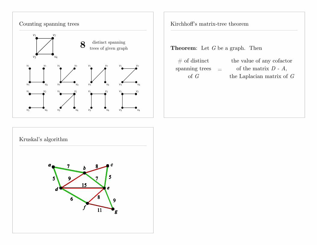
Counting spanning treesv1 v2

v3 v4

v1 v2

v3 v4

v1 v2

v3 v4

v1 v2

v3 v4

v1 v2

v3 v4

v1 v2

v3 v4

v1 v2

v3 v4

v1 v2

v3 v4

v1 v2

v3 v4

8 distinct spanning trees of given graph

Kirchho!’s matrix-tree theorem

Theorem: Let G be a graph. Then

# of distinct spanning trees

of G=

the value of any cofactor of the matrix D - A,

the Laplacian matrix of G

Kruskal’s algorithm

ab

c

d e

fg

7

7

8

515

5 9

6

11

98

ab

c

d e

fg

7

7

8

515

5 9

6

11

98

ab

c

d e

fg

7

7

8

515

5 9

6

11

98

ab

c

d e

fg

7

7

8

515

5 9

6

11

98

ab

c

d e

fg

7

7

8

515

5 9

6

11

98

ab

c

d e

fg

7

7

8

515

5 9

6

11

98

ab

c

d e

fg

7

7

8

515

5 9

6

11

98

ab

c

d e

fg

7

7

8

515

5 9

6

11

98

ab

c

d e

fg

7

7

8

515

5 9

6

11

98