Electronic copy available at: http://ssrn.com/abstract=1107998

Costly Information Processing: Evidence from Earnings Announcements∗

Joseph Engelberg¥

January 10, 2008

Abstract: I examine the role of information processing costs on post earnings announcement drift. I distinguish between hard information —quantitative information that is more easily processed — and soft information which has higher processing costs. I find that qualitative earnings information has additional predictability for asset prices beyond the predictability in quantitative information. I also find that qualitative information has greater predictability for returns at longer horizons, suggesting that frictions in information processing generate price drift. Using a tool from natural language processing called typed dependency parsing, I demonstrate that qualitative information relating to positive fundamentals and future performance is the most difficult information to process.

Key words: post earnings announcement drift, underreaction, information processing, financial media

∗ I have benefited from discussions with Torben Andersen, Nick Barberis, Paul Gao, Zhiguo He, Andrew Hertzberg, Ravi Jagannathan, Jiro Kondo, Robert Korajczyk , David Matsa, Jonathan Parker, Jared Williams and Beverley Walther. I am indebted to Mitchell Petersen and Paola Sapienza for advice and support. I also thank the Zell Center for Risk Research for its financial support. All errors are my own. ¥ Kellogg School of Management, Northwestern University, 2001 Sheridan Road, Evanston, IL 60208. Email: j- engelberg@northwestern.edu.

Electronic copy available at: http://ssrn.com/abstract=1107998

2

One of the most puzzling—and robust—challenges to the market efficiency hypothesis is the

evidence that security prices underreact to public news. Researchers have found evidence of

underreaction to earnings announcements (Ball and Brown (1968), Bernard and Thomas (1989, 1990)),

share repurchases (Ikenberry et al. (1995)), dividend initiations and omissions (Michaely et al. (1995)),

seasoned equity offerings (Loughran and Ritter (1995)), and stock splits (Ikenberry et al. (1996)). These

results are puzzling because an efficient market should incorporate all publicly available information

immediately; thus, future returns should not be predictable based on current information.

As the evidence has mounted for underreaction to information, many have begun to argue that the

assumption that financial agents have unlimited capacity to process information is too strong. If

information processing is costly, some information may not be immediately incorporated into prices.

Empirical papers that link costly information processing to underreaction have almost exclusively focused

on the idea that limited attention makes information hard to process at certain times. According to this

literature, limited attention may explain why underreaction to earnings announcements is greater on

Fridays (Della Vigna and Pollet, (2006)), when agents are distracted by other earnings announcements

(Hirshleifer et al. (2006)), among low volume stocks and in down markets (Hou et al. (2006)).

In this paper, rather than focusing on time series variation in attention, I focus on cross sectional

differences in the objective costs of information processing that are intrinsically embedded in each type of

information. The motivation behind this analysis is simple: information is not homogeneous in type.

While some news is easy to decipher and is incorporated quickly into market prices, other news requires

more costly processing and–depending on the size of the information processing costs–will be

incorporated into market prices only over time. For example, Plumlee (2003) argues that the complexity

of information is one reason why analyst forecasts may not incorporate public information. She shows

that the rate of incorporation of tax information into forecasts is decreasing in complexity.

To measure differential information processing costs, I classify news into hard/quantitative

information that is more easily processed and soft/qualitative information that is more costly to process.

To illustrate this point, consider the difference between evaluating a firm's income statement and the

transcript of its conference call. An income statement is made up largely of numbers organized in a

standardized fashion so that individuals can process it quickly and efficiently. A summary of its content

(like earnings per share) can be easily created, stored, compared to other firms, and transmitted. On the

other hand, the text of a conference call may not be so easy to process. Understanding its content may

take a sophisticated understanding of language, tone or nuance. A summary of its content may be more

difficult to create, more subjective, less comparable across firms, and more difficult to transmit. Similar

arguments about the processing costs of hard and soft information are given by Petersen (2004).

3

I study the differential effect of information processing cost in the context of earnings

announcements and the post-earnings announcement drift (PEAD). I choose this particular event as it

contains both hard and soft information, is repeated over time, and is the “granddaddy of underreaction

events” (Fama (1998)). To measure the qualitative content of the earnings surprise, I apply a method

introduced by Tetlock (2007) that counts the number of negative words as defined by the Harvard

Psychological Dictionary in the text of Dow Jones News Service (DJNS) stories about firms' earnings

announcements. To measure the quantitative content of the surprise, I use the Standardized Unexpected

Earnings (SUE), which is defined as the difference between firm earnings and the analyst median forecast

scaled by a normalization factor. I find that qualitative earnings information embedded in the DJNS has

additional predictability for asset prices beyond the predictability in SUE. The qualitative information

predicts larger price changes at longer horizons than SUE, consistent with the hypothesis that information

with high processing costs diffuses slowly into asset prices.

I then perform a series of robustness checks that exploit heterogeneity in the cross section of

investors and firms. With respect to investor heterogeneity, I find that stocks held by superior processors

of information–those with high institutional ownership–experience less predictability from costly

information. With respect to firm heterogeneity, I find that stocks in complex information environments–

high-tech firms and those with large R&D expense –experience more predictability from costly

information.

Finally, I explore the kind of soft information that is most difficult to process. Using a tool from

natural language processing called typed dependency parsing, I pair negative words with words that

belong to several different categories in order to identify the kind of qualitative information embedded in

the news reports that is most difficult to process. I find that qualitative information about positive

fundamentals and future performance is most important for the prediction of future returns; however, this

is not the case for analysts’ forecasts. To my knowledge, this is one of the few times natural language

processing —a way of processing language through models of sentence structure—has been used in

accounting or finance.1

My findings build upon several literatures. First, my results are consistent with Hong and Stein

(1999) where underreaction is modeled as the slow diffusion of information. Hong and Stein argue that

their model can be applied to public news if there is differential processing of that news. Although Hong

and Stein do not describe the channel by which information diffuses slowly and admit their mechanism

1 In the past, methods of machine learning like Naïve Bayes have been used (Antweiler and Frank (2003, 2004)). These methods search for the appearance of words in text in order to classify the text in predetermined categories. They differ from Natural Language Processing because they do not attempt to understand the meaning of the text, which requires, among other things, identifying parts of speech, sentence structure and grammar. Das and Chen (2007) consider several methods to classify sentiment in text including one method which identifies part of speech.

4

“may appear to be more ad hoc” relative to models built upon psychological biases, my results could be

described using their approach of modeling costly information processing as I illustrate in the Appendix.2

Second, there is a growing trend in the literature demonstrating the key role of the media as an

information intermediary (Huberman and Regev (2001), Dick and Zingales (2002, 2003), Miller (2006),

Tetlock (2007), Tetlock et al. (2007), Bushee et al. (2007), Bhattacharya et al. (2008) and Mullainathan

and Shleifer (2005)). My results are the first to show that the content of financial media can predict asset

prices in the medium term. Tetlock et al. (2007) explore similar themes, focusing on the information

content of financial media prior to the earnings announcement and finding that such content can predict

period-ahead SUE and next-day returns. However, the sample in Tetlock et al. (2007) concentrates on

S&P 500 firms. My sample has a shorter time series but a larger cross section of firms which I exploit in

cross-sectional tests. Finally, my paper relates to the corporate finance literature that analyzes the

differences in soft and hard information (Petersen (2004)) and their impact on lending decisions (Stein

(2002)). Whereas the corporate finance literature often argues that soft information increases the cost of

transmission and therefore affects corporate decisions, here I will argue that soft information’s increases

the cost of transmission and therefore affects asset prices.

Section I describes my data and variables. Section II examines the differential predictability of

hard and soft information in event time and calendar time and performs cross-section al tests. Section III

considers the market and analyst response to different categories of soft information. Section IV

considers alternative explanations for my findings. Section V summarizes my conclusions.

I. Description of Data and Variables

The data in this study come from five different sources. Compustat provides accounting

information and earnings announcement days. The Center for Research in Securities Prices (CRSP)

reports prices and returns. The Institutional Brokers Estimate System (I/B/E/S) supplies analyst forecast

data. CDA/Spectrum provides institutional holdings data. Article text for earnings announcement news

comes from the Dow Jones News Service (DJNS) as reported in Factiva, Unique identifiers in each data

source are matched to CRSP permnos.3

2 Although other models consider the cost of information acquisition (Grossman and Stiglitz (1980), Verrechia (1982) and Admati (1985)), these models are not concerned with explaining underreaction. A key difference between these rational expectation equilibrium (REE) models and a difference of opinion (DOO) model like Hong and Stein (1999) is the assumption in REE that agents can extract other agents’ information from prices. Banerjee et al. (2007) point out that price drift exists in standard DOO models but not in standard REE models. 3 Compustat's gvkey is matched to permno using CRSP Link (available through WRDS), I/B/E/S's ticker is matched to permno using the matched table generated by the sas program iclink.sas (avaliable through WRDS), CDA/Spectrum data are matched via cusip and Factiva's company code is matched to permno through a text matching program that I wrote (see the Appendix for details).

5

Firms included in the sample must have the following: a book value in Compustat and a market

value in CRSP at the end of the previous calendar year, an earnings announcement date in Compustat that

matches the date given in I/B/E/S, at least one analyst with an estimate no later than 50 days before the

earnings announcement date, and an article in the DJNS on the earning announcement day. These filters

create a sample of 51,207 earnings announcements from January, 4, 1999, to November 18, 2005, by

4,700 unique firms. This will be the sample of interest for the majority of the paper.

A. Description of Textual Data

Factiva is a database that provides access to archived articles from thousands of newspapers,

magazines, and other sources, including more than 400 continuously updated newswires such as the Dow

Jones newswires. A newswire is a service that transmits news stories, stock market results and other up-

to-the-minute information in electronic form to subscribers. The Dow Jones newswires are a collection of

wires covering all asset classes and reporting from more than 90 bureaus around the world. I choose the

Dow Jones News Service as the text for my analysis because it has been widely used in the literature and

has considerable coverage. According to Chan (2003), "by far the services with the most complete

coverage across time and stocks are the Dow Jones newswires. This service does not suffer from gaps in

coverage, and it is the best approximation of public news for traders."

i. Matching Firms to Articles

Studies that seek to relate media articles to firms face serious challenges in accomplishing this

task. First of all, it is hard to determine whether a firm is the subject of an article or merely mentioned in

passing. For example, a news story about AMD might mention Intel as its competitor or a story about

Alice Walton might mention that she drives a Ford. These are not stories about Intel or Ford and should

be distinct from stories that are. Secondly, some firms have names that are difficult to distinguish from

other firms, are different from their official company name, or resemble common English words. This

makes identifying the correct company—or whether a company is mentioned at all—problematic. For

example, articles might refer to Southwest Airlines as simply "Southwest" which makes it difficult to

distinguish from other companies with "Southwest" in their name. Articles often refer to Apple Inc. as

“Apple,” which makes it difficult to distinguish from the common word "apple." Moreover, it takes some

institutional knowledge of the catalogue of firms to understand how they might be referred to in an article.

For example, International Business Machines is almost always called IBM (which is also its ticker

symbol) whereas AMR Corp is almost always referred to by its popular subsidiary American Airlines.

6

The literature has addressed the problem of matching firms to articles in a variety of ways. Some

authors depend on the data provider to do the matching (Bushee et al. (2007), Antweiler and Frank

(2005)); some attempt to do the textual matching themselves (Tetlock et al. (2007)); some combine these

two strategies (Bhattacharya et al. (2008)); and some avoid describing how the matching is done (Chan

(2003)). I opt for the first approach and allow Factiva to do the matching for two reasons. First, by using

Factiva's indexing and not my own subjective judgment, the results in this paper can be replicated.

Second, Factiva has more expertise, manpower and computing power to do the matching. Since 1999,

Factiva has used a combination of computer technology and human editors to systematically assign

indexing codes to its articles identifying their key features in a process called Intelligent Indexing. These

features include the company or companies that are the subject of the article (see the Appendix for more

details). For each company, Factiva creates a unique identifier called a Factiva Company Code. I match

CRSP permnos to the Factiva Company Codes via an algorithm that makes a primary match based on

ticker symbol mentioned in the DJNS text and a confirming match based on the textual similarity of

company names (see the Appendix for more details).

However, there are two clear disadvantages to using Factiva's indexing. First, Factiva’s indexing

process is proprietary so I cannot know how it is done and how the process might influence my results.

Secondly, because Factiva only attaches a company code when it believes a company is the subject of an

article, I find that there are times when Factiva's threshold is too high. This non-indexing will lead to

some articles being left out of my sample.

ii. Predictability and Timing of Dow Jones News Service Articles

Because my sample is restricted to firm earnings announcements that appear in the DJNS, I first

examine the characteristics of firms and earnings news that predict coverage by the DJNS. I do this by

running a series of logistic regressions for whether an article appears in the DJNS or not. My results are

presented in Table 1. Of the 170,096 firm earnings announcement dates in Compustat for firms that I was

able to match Factiva codes with permnos, 80,935 (47.58%) had a story on the earnings announcement

day in the DJNS. Panels A and B suggest that both firm characteristics and story characteristics influence

coverage. Panel A indicates that firms with large market capitalizations and high analyst coverage are

most likely to receive coverage by the DJNS. A one standard deviation increase in log market

capitalization (analyst coverage) increases the odds of being covered by 50.2% (49.9%). Panel A

suggests that other characteristics such as a firm’s book-to-market ratio, idiosyncratic volatility, and

turnover appear unrelated to coverage by the DJNS. The strong correlation between market capitalization

and coverage is not surprising. Newswire reporters cater to their clients, and firms with large market

7

capitalization are most likely to have a larger base of shareholders and clients of the DJNS.4 Additional

evidence for this fact comes from Panel B. Since the DJNS is available through terminals like Bloomberg

and Thompson ONE, the DJNS is most likely to have institutional (rather than retail) clients. When I

consider the dollar amount of market capitalization held by institutions and non-institutions using

CDA/Spectrum data, I find that the market capitalization associated with institutions is more important

for determining coverage by the DJNS. A one standard deviation increase in the log market capitalization

held by institutions (the log market capitalization not held by institutions) increases the odds of being

covered by 57.0% (2.70%). These results suggest that the DJNS considers demand for their service when

determining which stories to cover. The fact that there is a positive relationship between analyst coverage

and DJNS coverage suggests that reporters consider supply as well. Reporters need sources for their

stories, and a firm with many analysts has a larger potential supply of sources than a firm with few

analysts. However, it is also possible that analyst coverage proxies for some omitted demand-related

variables. The same demand-related variables that lead analysts to cover firms might lead reporters to

cover the same firms.

Panels A and B include industry dummies, and although the coefficients on the 49 dummies are

omitted for brevity, a Wald Test that tests the joint hypothesis that the coefficients on the industry

dummies are jointly zero is rejected at the one percent level. Coverage in the DJNS appears to favor the

automobile, steel and wholesale industries and disfavor the telecom, software and banking industries.

News characteristics are also important for determining coverage, although their economic

significance is smaller than that of the market capitalization and analyst coverage. Firms with extreme

returns are more likely to receive coverage, and this result is slightly asymmetric. For positive abnormal

returns, a one standard deviation increase corresponds with a 12% increase in the probability of coverage.

For negative abnormal returns, a one standard deviation decrease corresponds with a 8.81% increase in

the probability of coverage.5

Figure 1 plots the distribution of DJNS articles in my sample throughout the day. Consistent with

past studies that find most corporate disclosures are released outside of U.S. market hours (Patell and

Wolfson (1982)), I find the media articles covering earnings announcements are also concentrated outside

of market hours. Figure 1 is bimodal with peaks at 8:00 a.m. and 4:00 p.m. EST. During market hours,

the fewest number of earnings stories occur around 1:30 p.m.

4 Some newswire reporters with whom I spoke claimed there was a market capitalization threshold which determined whether they would cover firms. However, I found no evidence of such a threshold in my data. 5 Positive abnormal returns are defined as max(0, CAR[-1,1]) and negative abnormal returns are defined as min(0, CAR[-1,1]). If I insert an indicator variable for whether the abnormal return was positive (or negative), its coefficient becomes economically and statistically insignificant.

8

B. Defining Hard and Soft Measures of Earnings News

Although the concept of hard and soft information has existed in finance literature for quite some

time, there is no rigorous definition of what distinguishes the two. Instead, as Petersen (2004) argues, we

should consider classifying information along a continuum between hard and soft and allow certain

properties of information to determine where a particular piece of information falls along the continuum.

Soft information is often communicated with text; thus, it is costly to store, more subjective, and difficult

to pass along without loss of information. In contrast, hard information is often communicated with

numbers; thus, it is more objective and easily comparable. An individual’s height, an equity return, and a

bond rating are all examples of hard information. A movie review, an interview of a loan applicant, and

the text of a conference call are all examples of soft information.

Using this as a foundation, I define hard and soft content of earnings news. Hard earnings news

will be based on the accounting data (earnings) released at the earnings announcement, whereas soft

earnings news will be based on the text of media articles written about the earnings announcement.

Earnings data are quantitative, easily comparable across firms (e.g., $3 EPS versus $4 EPS), independent

of who collects it, easy to store and easily passed on without loss of information. The textual data is

qualitative, not easily comparable across firms (e.g., it is not easy to compare “demand is weak” with

“management is inexperienced”), dependent upon who collects it (e.g., not everyone may agree that

“demand is weak”), and thus, difficult to interpret, store and pass on without loss of information.

i. Soft Measure of Earnings News

My soft measure of earnings news is very similar to that used by Tetlock (2007) who examines

the qualitative content of financial media. Tetlock uses a program called the General Inquirer (GI) to

count the number of times words occur within text from predetermined categories as determined by the

Harvard IV-4 psychological dictionary. Although there are 77 different word categories in the dictionary

ranging from "pain" to "expressive" to "virtue", Tetlock finds that words from the "negative" category

predict both one-day market returns and firm-specific returns. Like Tetlock, I only consider negative

words in my analysis since it appears they capture qualitative information better than positive words.

Tetlock explains that this might be the case if negations ("no", "not", etc.) are more often paired with

positive words than negative words. However, I find very few negations in the DJNS. A critical purpose

of a newswire service is to communicate information quickly and efficiently, and it is more efficient to

write "bad" than "not good." The failure of positive words in qualitative language analysis may be caused

by the large number of common financial terms that are erroneously classified as positive.6

6 For example, consider the sentence: "Dell is a terrible company with 100 shares outstanding" which contains the commom financial terms "company", "shares" and "outstanding." The General Inquirer will classify each of those

9

I download the headline and lead paragraph of DJNS articles from Factiva through a computer

program that systematically sends queries to Factiva's database. Using the headline and lead paragraph

from the Dow Jones News Service takes advantage of the practice by journalists of summarizing the

articles content in the headline and lead sentence (King and Loi [2003]). I count the fraction of negative

words as defined by the Harvard Psychological Dictionary in the DJNS article on the earnings

announcement day. Formally, I define the fraction of negative words as7:

Negative Fractionit = ( (total negative words for firm i on day t)/ (total words for firm i on day t) )

For multiple articles on the same earnings announcement day, I combine the headline and lead paragraph

from each article and count the fraction of negative words. As an illustration, consider the DJNS article

that followed Dow Chemical's earnings announcement on January 28, 1999. The headline and lead

paragraph read:

DOW CHEM 4Q SUFFERS FROM LOW PRICES; PROBLEM TO PERSIST. Dow

Chemical Co. (DOW) reported fourth quarter profit that shrunk from year ago levels and

continuing low chemical prices will likely undermine any near term turnaround.

The headline and lead paragraph contain 36 words, five of which are classified as negative: "suffers",

"problem", "undermine" and "low" (two times). For this observation the value of Negative Fraction is

5/36 = .139 and is among the most negative in my sample (in the 97th percentile). This crudely captures

the fact that the soft information in the article is considerably negative.

ii. Hard Measure of Earnings' News

For a quantitative measure of earnings news, I calculate Standardized Unexpected Earnings

(SUE), where expected earnings are defined relative to the median analyst forecast.8 Formally:

terms as positive and only “terrible” as negative. (see http://www.webuse.umd.edu:9090/GI?sentence=Dell+is+a+terrible+company+with+100+shares+outstanding.%0D%0A). The sentence will appear considerably positive although its sentiment is negative. 7 Tetlock et al. (2007) consider year-over-year changes in Negative Fraction and standardize by the standard deviation of negative words in each year. My results remain qualitatively unchanged when I define Negative Fraction in this way as well. 8 Other papers (e.g., Bernard and Thomas (1989)) use a time series model. Such a model uses the prior calendar year's quarter-matched earnings and standardizes by the historical standard deviation of unexpected earnings defined in this way. Kothari (2001) argues "...in recent years it is common practice to (implicitly) assume that analysts' forecasts are a better surrogate for market's expectations than time-series forecasts." Mendenhall (2006) shows that

10

SUEit = UEit/σy-1 = (Ait - Eit) / σy-1

where Ait is the actual (unadjusted by splits or dividends) EPS as reported by I/B/E/S for firm i on day t,

Eit is the median of the analysts' forecasts in the last survey before the earnings announcement that is less

than 50 days before the announcement, UEit = (Ait - Eit) is defined as the unexpected earnings, and σy-1 is

the standard deviation of the unexpected earnings in the previous calendar year.

C. Calculation of Abnormal Returns

To evaluate whether a stock has superior or inferior performance following an earnings

announcement, I establish a benchmark return and calculate an abnormal return as deviation from the

benchmark. As Vega (2006) notes, the choice of the appropriate benchmark return has varied over time.

Some authors simply use the market return or a size-matched portfolio return, while others estimate factor

loadings outside an event window in some model specification (like the Fama-French three factor model)

and use the factor observations inside the event window to estimate a benchmark return. Barber and Lyon

(1997) and Daniel and Titman (1997) argue that benchmark returns calculated using matched book-to-

market and size sorted portfolios result in better test statistics, and I adopt this approach.9

To construct the matched book-to-market and size sorted portfolios, I follow the approach of

Fama and French (1992). In each year, I collect the market capitalization of each firm at the end of June

according to CRSP, and the book value of each firm at the end of December of the prior year according to

Compustat. I use these to calculate book-to-market quintile breakpoints and size quintile breakpoints and

sort the universe of firms into 25 bins. For every firm, this will specify its matched portfolio from July to

June of the next year when the process will repeat. The abnormal return for each firm is then defined as

the difference between that firm's return and the matched portfolio return. Formally:

ARit = Rit - Mit

where ARit is the abnormal return for firm i on day t, R_it is the equity return, and Mit is the matched

portfolio return. Then the cumulative abnormal return (CAR) for firm i in calendar quarter q beginning

on event day a and ending on day b is:

CARiq[a,b] = ∑=

=

bt

atiqtAR

PEAD is larger when unexpected earnings are defined using analyst forecasts. My results throughout the paper do not change qualitatively when I use a time series model to estimate the quantitative earnings surprise. 9 I also replicated the results herein by defining the abnormal return as the difference between the actual return and the Fama-French three factor benchmark. For brevity, I do not report these results, but they are qualitatively similar.

11

Throughout the paper a and b will be specified in event time where the event is an earnings

announcement. For example, CAR[2,81] is the sum of 80 abnormal returns beginning the second day

after the earnings announcement. The q subscript is included because firms make multiple earnings

announcements in my sample.

D. Summary Statistics

Table 2 Panel A includes summary statistics for Negative Fraction. 47.5% of my observations

have no negative words in the headline or lead paragraph. The mean (median) fraction of negative words

in my sample is 3.6% (1.8%) with a standard deviation of 4.6%. As Panel B illustrates, Negative Fraction

has little correlation with other variables associated with earnings surprise: SUE and CAR[-1,1]. The

correlation between CAR [-1,1] is -.06 and the correlation between Negative Fraction and SUE is -.09. In

comparison, the correlation between SUE and CAR [-1,1] is .19. Negative Fraction also appears to have

little correlation with other variables linked to PEAD, including size (log market capitalization),

dispersion of beliefs (standard deviation of analyst forecasts and average turnover), uncertainty

(idiosyncratic volatility) and price momentum (40-day CAR before announcement).

My sample is biased against small firms since both financial media and analysts are more likely

to cover large firms. The average firm in my sample is larger than the average firm in CRSP. This

statistic is shown in Panel C, which plots the yearly log market capitalization of the median firm in my

sample and the median firm in CRSP. Panel C illustrates that a firm in the 75th percentile of the CRSP

universe is about the size of a median firm in my sample. The median (lower quartile, upper quartile)

market capitalization of a firm in my sample grew from $413 million ($117 million, $1.67 billion) in

1999 to $1.19 billion ($370 million, $4.03 billion) in 2005.

II. Does Soft Earnings News Contain Information in Addition to SUE?

Firms announce much more than earnings-per-share at an earnings announcement (Rajgopal,

Shevlin and Venkatachalam (2003), Gu (2004)). For example, there is often a lengthy press release that

accompanies an income statement, and firms often hold conference calls to address questions about

performance. Along with interviews of managers, analysts, and shareholders, these qualitative data are

important inputs for journalists who write articles about the summary of a firm's earnings announcement.

Before I can examine the differential predictability of quantitative and qualitative information, I must

show qualitative content has some additional predictability and that this predictability is captured by

Negative Fraction.

12

A. Event-time Abnormal Returns

I first examine PEAD for different SUE quintiles. In each calendar quarter, I use the previous

period's calendar quarter to determine quintile cutoffs for SUE. I then sort each earnings surprise into its

appropriate SUE bin and examine the 80-day CAR that follows.

The upper panel of Table 3 provides evidence that PEAD exists in my sample. The size of PEAD

increases almost monotonically across the SUE quintiles with the lowest quintile experiencing an average

80-day CAR of -0.60% and the highest quintile experiencing an average 80-day CAR of 1.90%. The

difference of 2.59% is statistically significant under both a parametric two-sample t-test and the non-

parametric Wilcoxon sum rank test (which tests whether the Hodges-Lehman measure of central tendency

is non-zero). The size of PEAD is small relative to older studies (Bernard and Thomas (1989)) and is

consistent with more recent studies (Brandt et al. (2006)).

To see whether the qualitative measure of earnings contains information related to PEAD, I

further sort each quintile into bins based on Negative Fraction. The first bin is for articles that have no

negative words (Negative Fraction = 0%), the second bin is for articles where 0-5% of words are negative

(0 < Negative Fraction ≤ 5%), and the third bin is for the remaining articles (Negative Fraction > 5%). I

sort on absolute values of Negative Fraction rather than quartiles or quintiles, because almost half of the

articles have no negative words in the headline and lead paragraph. Sorting on the measure of soft

information creates dispersion in future returns within SUE quintiles, and the results are most pronounced

for the higher SUE quintiles. For example, within SUE quintile 5, the average 80-Day CAR is 3.90% for

firms with Negative Fraction = 0 and .28% for firms with Negative Fraction > 5%. Within SUE quintile

4, the average 80-Day CAR is 2.28% for firms with Negative Fraction = 0 and -1.23% for firms with

Negative Fraction > 5%.

These results suggest that the qualitative information embedded in the DJNS contains information

in addition to SUE, and that, like SUE, this information is not immediately incorporated into prices. The

concentration of Negative Fraction's predictability in high-SUE quintiles is also interesting. If negative

words are being used about a firm with a low SUE, those negative words might simply be reiterating the

content of the quantitative negative surprise. In other words, in low SUE bins the qualitative measure

may simply mirror the quantitative measure. However, in high SUE bins, the presence of negative words

makes it more likely the qualitative measure is adding new information (since a description of a positive

earnings surprise is less likely to have negative words). Such an observation makes it tempting to

examine the additional predictability of positive words in low SUE bins. However, as discussed in

Section I.B, there is a noisiness inherent in positive words. The predictability of positive words in a

regression framework is discussed in the Appendix.

13

Table 4 demonstrates my results in a linear regression framework with additional controls. The

dependent variable is CAR[2,81], and the key independent variables are the accounting surprise SUE, the

market response CAR[-1,1], and Negative Fraction. I include additional variables to control for other

variables related to PEAD. The literature has found PEAD is most pronounced for small firms, so I

include Log Market Cap and (Log Market Cap * SUE); for firms with high differences of opinion so I

include Average Turnover and (Average Past Turnover * SUE)10; for firms with high information

uncertainty so I include Idiosyncratic Volatility and (Idiosyncratic Volatility * SUE) and for firms with

low analyst coverage so I include Number of Analysts and (Number of Analysts * SUE). I also include

the Fama-French 49 industry dummies, because certain industries may be more likely to use negative

words than others. SUE, CAR[-1,1], Log Market Cap, Average Past Turnover, Idiosyncratic Volatility,

and Number of Analysts are all de-meaned in order to better interpret the coefficients on the main effects.

Specifically, the coefficients on the independent variables can be interpreted as the dependent variable’s

sensitivity to a unit change in the independent variable conditional on all other variables being set to their

mean. Standard errors reported in Table 4 (Panel 1, Panel 2) are robust and clustered by the (earnings

announcement date, calendar quarter of the earnings announcement) to allow for correlation in error

terms.11

In this linear regression framework, I find that Negative Fraction, CAR[-1,1] and SUE all predict

CAR over the next 80 days. Assuming all other variables are set to their mean, a one standard deviation

increase in Negative Fraction (CAR[-1,1], SUE) leads to a 79 bps (65 bps, 47 bps) increase in CAR over

the next 80 days. As Tetlock et al. (2007) admit and is intuitively clear, Negative Fraction is a rather

crude measure of the content of textual information given that measurement error will bias its coefficient

downward. Despite this, Negative Fraction bears a remarkably economically significant predictive power

relative to SUE and CAR[-1,1].

10 Using the standard deviation of analyst forecasts as an alternative measure of difference of opinion does not qualitatively change any of the results. I do not use this variable as a control because it reduces my sample size by about 15% (the standard deviation of analyst forecasts is not defined for firms followed by one analyst). 11 I cluster the standard errors in this way after investigating features of the panel data as suggested by Petersen (2008). For example, in Panel 2 of Table 4 the dependent variable is CAR[2,81] and the independent variables of interest are Negative Fraction, CAR[-1,1] and SUE. The robust standard errors without clustering in any dimension for (Negative Fraction, CAR[-1,1] and SUE) are (.02996, .02059, .00151). After clustering the errors by firm, I find no qualitative change in standard errors: (.03226, .02022, .00154) which suggests there is no substantial firm effect in the data (permanent or temporary). When I cluster the standard errors by calendar quarter, they increase to (.06848, .03651, .00205). I find similar results when I cluster by “majority quarter” (the calendar quarter in which the majority of CAR[2,81] falls). If I include calendar quarter dummies rather than cluster the errors by calendar quarter, I find the standard errors of the variables of interest to be (.02967, .02066, .00152). This suggests the presence of a non-constant time effect in the data (see Petersen 2008).

14

B. Calendar-time Returns

Cumulative abnormal returns in a panel data setting do not have the interpretation of profits from

a trading strategy, so I consider the profits from five trading strategies based on Negative Fraction, CAR[-

1,1] and SUE:

Strategy 1: Going long firms in the highest SUE quintile and short firms in the lowest

SUE quintile.

Strategy 2: Going long firms with Negative Fraction = 0 and short firms with Negative

Fraction > 5%.

Strategy 3: Going long firms in the highest CAR[-1,1] quintile and short firms in the

lowest CAR[-1,1] quintile.

Strategy 4: Going long firms in the highest SUE quintile with Negative Fraction = 0 and

short firms in the lowest SUE quintile with Negative Fraction > 5%.

Strategy 5: Going long firms in the highest CAR[-1,1] quintile with Negative Fraction =

0 and short firms in the lowest CAR[-1,1] quintile with Negative Fraction > 5%.

Positions are opened two days after the earnings announcement and held for 40 days in the top panel.

Positions are opened 42 days after the earnings announcement and held for 40 days in the bottom panel.

The daily return from each strategy is the equally weighted return of the securities that make up the

position.12

The daily profits from each strategy are then regressed against the Fama-French three factors and

a momentum factor.13 The details from these regressions are reported in Table 5. For all five strategies,

the loading on the momentum factor is positive and significant. This is consistent with previous studies

that suggest that the momentum factor explains some – but not all – of the profits from a PEAD strategy

(Chan et al. (1996), Chordia and Shivakumar (2006)). The returns to Strategies 2, 4 and 5 that

incorporate soft earnings news load more negatively on the Fama-French Small-Minus-Big (SMB) factor,

which suggest that this strategy overweights large firms. Concerning profitability, all five trading

12 Equally weighting the composite returns assumes constant rebalancing of the securities which make up the portfolio. Weighting by the cumulative return of the composite securities in the portfolio (i.e. assuming no rebalancing) has little effect on my results. 13 The daily returns to each of the four factors are taken from Ken French’s website at: http://mba.tuck.dartmouth.edu/pages/faculty/ken.french/data_library.html

15

strategies generate statistically and economically meaningful profits at some horizon. Strategy 1 is based

only on SUE and generates a statistically significant daily alpha of 2.3 bps (48 bps a month) in the first 40

days but a statistically insignificant daily alpha of 0.5 bps (11 bps a month) in the next 40 days. Strategy

2 is based only on Negative Fraction and generates a statistically insignificant daily alpha of 1.3 bps (27

bps a month) in the first 40 days but a statistically significant daily alpha of 3.1 bps (65 bps a month) in

the next 40 days. Strategies 4 and 5 suggest combining information in the announcement return or SUE

with the soft information in Negative Fraction can lead to additional trading profits. For example,

Strategy 4 is based on SUE and Negative Fraction and generates daily alpha of 4.7 bps (99 bps a month)

in the first 40 days and daily alpha of 2.9 bps (61 bps a month) in the next 40 days. These results provide

additional evidence that the soft earnings news in Negative Fraction generates additional predictability for

future returns.

Having established that the qualitative earnings news contains information in addition to SUE

and CAR[-1,1], I next examine the timing of that additional information's incorporation into prices.

C. The Timing and Magnitude of the Predictability of Hard and Soft Earnings Information

As I argue in Section I.B using Petersen (2004), soft information is costly to process relative to

hard information. Because Negative Fraction is my proxy for the content of soft earnings news and SUE

is my proxy for the content of hard earnings news, I interpret the differential predictability of Negative

Fraction and SUE as the effect of costly information processing. If information is costly to process, then

soft information should diffuse slowly into asset prices relative to hard information. While interpreting

the differential predictability of hard and soft earnings news, the reader should keep in mind the relative

measurement error of Negative Fraction and SUE. In the forthcoming regressions, measurement error

will undoubtedly bias downward the estimated coefficient on Negative Fraction. This fact, however, will

work against any results I find. My results will likely be understated to the extent that I find greater

predictability of future returns from Negative Fraction relative to SUE.

My results are presented in Table 6. In each regression, I include the same controls for log

market capitalization, analyst coverage, idiosyncratic volatility, average past turnover, and industry as in

Table 4. All variables are also demeaned to better interpret the coefficients on the main effects. When

CAR[2,41] is the dependent variable, SUE has greater predictive power than Negative Fraction. A one

standard deviation change in SUE corresponds with a 52 bps change in CAR[2,41], whereas a one

standard deviation change in Negative Fraction corresponds with a 24 bps change in CAR[2,41], and only

SUE is statistically significant (at the 1% level). When CAR[42,81] is the dependent variable, Negative

Fraction has greater predictive power. A one-standard deviation change in SUE corresponds with a 5 bps

change in CAR[42,81], whereas a one standard deviation change in Negative Fraction corresponds with a

16

55 bps change in CAR[42,81], and only Negative Fraction is statistically significant (at the 5% level).

Figure 2 illustrates the above results in the 80 days after the earnings announcement. The top line plots

the difference in average CAR between SUE quintile 5 and SUE quintile 1 in event time. The bottom line

plots the difference in average CAR between the low (Negative Fraction = 0) and high (Negative Fraction

> 5%) bins for Negative Fraction. The figure demonstrates the differential predictability of the

quantitative and qualitative measures of earnings news in event time.

The third panel of Table 6 points to the source of the predictability of Negative Fraction in the

second 40 days after the earnings announcement. Among SUE, Negative Fraction, and CAR[-1,1], only

Negative Fraction is a statistically significant predictor of the next earnings announcement return. Table

4 also demonstrates that Negative Fraction continues to be a predictor of earnings announcement

abnormal returns two, three and four quarters ahead. A one standard deviation in Negative Fraction

predicts a 22 (25, 14) bps increase in earnings announcement abnormal returns two (three, four) quarters

ahead, whereas a one standard deviation in SUE predicts a 13 (7, 3) bps increase in these returns.

Taken together, the results provide evidence that the return predictability from Negative Fraction

is larger and occurs further away from the earnings announcement relative to SUE. I interpret this as

evidence that Negative Fraction is more costly to process than SUE and that costly information diffuses

more slowly into asset prices.

D. Sorts on Institutional Ownership

I have thus far argued that soft information is costly to process, and this underlying theme has

been the driving force behind my results in the previous sections. Here I consider the predictability of

soft information among firms with varying levels of institutional ownership. This analysis has two

underlying assumptions: (1) that institutions are better processors than individuals, because they have

more resources to process information; and (2) that equity-holders scrutinize the information of the stocks

they hold.14 If this is the case, we should expect to find less predictability from soft information among

stocks held by institutions.

I perform a series of cross sectional regressions to test this hypothesis. Institutional data are from

CDA/Spectrum Institutional Holdings data gathered from 13f forms filed with the SEC. Institutional

holdings are defined as the total amount held by institutions who file 13f forms divided by total shares

outstanding at the beginning of the calendar quarter of the earnings announcement.

14 Although the second assumption seems intuitive, it is also plausible if there are limits to arbitrage in the form of short-selling. If the costs of shorting a stock are high, then processing information about owned stocks has a distinct advantage over those that are not owned because, in the case of no ownership, negative information may not be able to be acted upon.

17

My results are in Table 7, and they support the hypothesis. When CAR[2,81] is the dependent

variable, the coefficient on Negative Fraction declines almost monotonically from the low institutional

ownership bin to the high institutional ownership bin. The coefficient on Negative Fraction in the lowest

(highest) bin is -0.2705 (-0.044). The coefficient on Negative Fraction in the lowest bin is significantly

different from zero (t-stat -2.36), but the coefficient on Negative Fraction in the highest bin is

indistinguishable from zero (t-stat -0.54). My results are similar if the dependent variable is the abnormal

return around the subsequent earnings announcement.

An alternative interpretation of these results is that newswire reports are only available to

institutions. Access to the DJNS is by paid subscription and is often retrieved via a terminal like

Bloomberg or Thompson ONE. I view this as a distinction but not a difference. Costly information

acquisition has two apparent key components: the cost of accessing data and the cost of processing those

data into information about discounted future cash flows (“information processing”). It may be that the

information cost that institutions bear comes from at least one of these components.

E. Sorts on R&D Expense and High-Tech Firms

In the previous section I sorted the cross section of firms by institutional ownership with the idea

that institutions are better processors of information. Here I sort the cross section of firms by the

complexity of the information environment with the idea that soft information will be more costly among

firms with newer production technologies. I approach this in two ways. First, I sort by R&D expense (as a

fraction of total expense) and rerun my baseline regressions in each R&D quintile. Second, I use the

American Electronic Association’s classification of high-tech firms and rerun my baseline regressions

among high-tech and non high-tech firms.15

The results are in Tables 8 and 9, and they suggest that soft information has greater predictability

among firms with complex information environments. When the dependent variable is CAR[2,81], the

coefficient on Negative Fraction is -0.5779 (-0.0138) in the quintile of firms with the highest (lowest)

fraction of R&D expense. To understand the relative economic magnitude of these coefficients, a one

standard deviation increase in Negative Fraction among high R&D firms corresponds to a 278 bps

increase in CAR[2,81], whereas a one standard deviation increase in Negative Fraction among low R&D

firms corresponds to a 6 bps increase in CAR[2,81]. I find similar results concerning the relative

magnitude of coefficients when the dependent variable is the abnormal return around the subsequent

earnings announcement. I also find vastly different coefficients on Negative Fraction among high-tech

15 The AeA considers the following SIC codes High-Tech: 3571, 3572, 3575, 3577, 3578, 3579, 3651, 3652, 3661, 3663, 3669, 3671, 3672, 3675, 3676, 3677, 3678, 3679, 3674, 3821, 3822, 3823, 3824, 3825, 3826, 3829, 3827, 3861, 3812, 3844, 3845, 4812, 4813, 4822, 4841, 4899, 7371, 7372, 7373, 7374, 7375, 7376, 7377, 7378, 7379. See http://www.aeanet.org/Publications/IDMK_definition.asp#List.

18

and non high-tech firms. When the dependent variable is CAR[2,81], the coefficient on Negative Fraction

is -0.5893 (-0.0606) among high-tech (non high-tech) firms.

F. Sorts on Idiosyncratic Volatility

As Shleifer and Vishny (1997) point out, agents may not trade on information they have if they

face limits like arbitrage risk or short-selling constraints. Here I consider whether the profitability from

soft information is related to arbitrage risk. While this will not explain why the market underreacts to soft

information, it helps to explain why this underreaction is not arbitraged away. To proxy for arbitrage risk,

I use idiosyncratic volatility, which is the most common proxy in the finance literature. I define

idiosyncratic volatility as the standard deviation of abnormal returns in the 40 days before the earnings

announcement. My results are reported in Table 10. When CAR[2,81] is the dependent variable, the

coefficient on Negative Fraction declines almost monotonically from the low idiosyncratic volatility

quintile bin to the high idiosyncratic volatility quintile bin. The coefficient on Negative Fraction in the

lowest (highest) bin is 0.0544 (-0.5444). The difference in magnitude is both statistically and

economically significant. A one standard deviation increase in Negative Fraction among high volatility

firms corresponds to a 257 bps increase in CAR[2,81], whereas a one standard deviation increase in

Negative Fraction among low volatility firms corresponds to a 22 bps increase in CAR[2,81].

III. Categories of Soft Information

Thus far I have shown evidence that soft information predicts returns around subsequent earnings

announcements. Not all soft information is the same, so here I consider what kind of soft information

predicts returns. This analysis can sharpen our understanding of costly information processing, because it

examines what kind of soft information is most difficult for the market to process.

At first glance, it might seem as if subject categorization techniques used in the prior literature

(Antweiler and Frank (2003, 2005)) would be an appropriate approach. This approach would sort each

article into predefined subjects. For example, consider the sentence: “Although sales remained steady,

the firm continues to suffer from rising oil prices.” Based on key words in the sentence, with

categorization techniques I could know that the sentence is negative and it concerns sales and oil prices.

But this is not enough. In order to refine my analysis, I need to know that the negative sentiment is about

oil prices. Identifying this relationship requires an understanding of the sentence structure, grammar and

part of speech. Tools designed to do exactly that belong to a broad discipline that joins linguistics and

computer science called Natural Language Processing (NLP).

19

For my analysis, I use the Stanford Parser to perform typed dependency parsing.16 Typed

dependency parsing refers to the decomposition of a sentence into a series of relationships between

individual words from a set of grammatical relation types. For example, the sentence, "The sluggish

economy created the decline," can be parsed into a series of word relations17:

Word Pair Relation

(economy, the) "the" is a determiner which modifies "economy"

(economy, sluggish) "sluggish" is an adjective which modifies "economy"

(created, economy) "economy" is a nominal subject with argument "created"

(decline, the) "the" is a determiner which modifies "decline"

(created, decline) "decline" is the direct object of "created"

I use the Stanford Parser to find the typed dependencies that include the negative words in the

text. In other words, I am not only interested in whether the text contains the negative word

"disappointing" but also in what the word "disappointing" relates to. For example, if "disappointing"

modifies the word "sales" then my soft information may concern positive fundamentals, but if

"disappointing" modifies the word "outlook" then my soft information may have to do with future

performance. Unfortunately, there are no word list categories that I know of that might divide earnings

news into categories, so I create six categories: positive fundamentals, negative fundamentals, future

outlook, environment, operations, and other.18

For each category on each earnings announcement date, I divide the sum of grammatical relations

among the set of negative words and words in the category by the total number of relations in the text.

For a sentence with N words, there will be N-1 grammatical relations generated by the parser. Using the

16 The Stanford Parser is available at http://nlp.stanford.edu/software/lex-parser.shtml 17 The output from the Stanford Parser codes these relations as: det(economy-3, the-1), amod(economy-3, sluggish-2), nsubj(created-4, economy-3), det(decline-6, the-5) and dobj(created-4, decline-6). The text before each abbreviation indicates the type of relation (e.g. "amod" stands for adjective modifier) and the numbers after the dashes indicate the position in the text. There are a total of 48 grammatical relations (see http://nlp.stanford.edu/pubs/LREC06_dependencies.pdf for the complete list) which the parser can assign. 18 Words I associate with positive fundamentals are: earnings, sales, results, revenue, profit and income; words I associate with negative fundamentals are: costs, expenses, spending, and charges; words I associate with future outlook are: guidance, outlook, plans and forecast; words I associate with environment are: demand, environment, conditions, economy, customers and competition; words I associate with operations are: business, operations, production, product, division and services. Other includes all words not in the other five categories. For each word in each category, I include all words whose word "stem" maps to the word. For example, along with the word "forecast", I include "forecasts", "forecasted", "forecasting", "forecaster" and "forecasters."

20

sentence above as an example, environment = (1/5), because one of the five relations in the text is

between a negative word ("sluggish") and a word in the environment category ("economy").

I replace Negative Fraction with the six new variables in my baseline regression to predict

CAR[2,81] and the abnormal return around the subsequent earnings announcement, and I report my

results these results in Table 11. The coefficient on each of my six variables are negative with the

exception of negative fundamentals. This makes sense, because negative words in relation to words like

"costs" and "expenses" can have either positive meaning (e.g. "low costs") or negatives ones (e.g.

"disappointing costs"). Of the other five categories, only positive fundamentals, future, and other have

statistically and economically significant negative coefficients. In other words, soft information about

positive fundamentals and future performance are most predictive of future returns. The fact that the

coefficient on other is significant suggests that there are additional categories of soft information that

predict future returns that have yet to be identified. Taken together these results suggest that some of the

information that is most difficult to process relates to current positive fundamentals and future

performance. Moreover, there are additional unidentified categories of information that are also difficult

to process.

A. Analyst Response to Soft Information

The above results suggest that there are certain important categories of soft information that are

not incorporated into prices. To explore these results further, I consider how analysts respond to soft

information. To do this, I consider the effect of soft information in quarter t on the median analyst

forecast for quarter t + 1. Specifically, I let Change in Estimate at quarter t = (the median analyst estimate

for quarter t + 1’s earnings in the first I/B/E/S survey after quarter t’s earnings announcement) – (median

analyst estimate for quarter t + 1’s earnings in the last I/B/E/S survey before quarter t’s earnings

announcement).19 This variable captures how the information in quarter t’s forecast affected the analyst’s

estimate of quarter t + 1. I then perform my baseline regression with Change in Estimate as the

dependent variable in Panel A of Table 12 and consider categories of soft information in Panel B.

Panel A suggests that analysts do respond to soft information, although the economic significance

of Negative Fraction is dwarfed by that of SUE and CAR[-1,1]. The standardized coefficient on SUE and

CAR[-1,1] is about 10-12 times larger than the standardized coefficient on Negative Fraction. This could

be due to the measurement error of Negative Fraction, or it could suggest that the information in SUE and

CAR[-1,1] is easier for analysts to process. Panel B provides some evidence for the latter. Recall from

19 In untabulated results, I have also considered defining Change in Estimate as the difference in mean estimates, scaling it by price or making it a ternary variable with values (-1,0,1) to represent (decrease, no change, increase). My results do not change qualitatively in each specification.

21

Table 11 that of the six earnings categories I identify, soft information about positive fundamentals and

the future seem to be most important for predicting future returns. However, neither coefficient is

statistically significant in Panel B, and environment is the only one of the identifiable categories that has

bearing in this case. In other words, the two categories of soft information that seem to be most important

for future returns appear less important to analysts. This suggests a possible channel by which this

information fails to get into prices. However, the Other category predicts both the change in analyst

forecasts as well as future returns so that there is some evidence that analysts do correctly incorporate yet-

to-be determined categories of soft information which are important for future returns.

IV. Alternative Explanations/Robustness Checks

A. Soft Information as a Measure of Accruals

I have argued that negative fraction captures the qualitative content of earnings surprises, but it is

also possible that Negative Fraction captures other pieces of hard information that have been shown to

predict future returns. For example, it is well known in the accounting literature that positive (negative)

accruals predict negative (positive) future returns, and that the predictability from accruals is distinct from

PEAD (Collins and Hribar (2000)). In untabulated results, I find that the correlation between Negative

Fraction and quarterly accruals as defined in Collins and Hribar (2000)20 is -.038 and that including

accruals into the baseline regressions of Tables 4 and 6 does not qualitatively change the results.

B. Regulation Fair Disclosure and the Bubble Period

The time period of my sample includes two key events that might affect the results: the bursting

of the “Internet Bubble” in March of 2000 and the implementation of Regulation Fair Disclosure (Reg

FD) in October of 2000. For example, it is possible that before Reg FD, financial journalists were able to

obtain private information from firms. This would explain the predictability of Negative Fraction

(although it would not explain why investors do not immediately incorporate this information after it is

reported by journalists) and why soft information was only important during the Internet Bubble when

traditional measures of performance were being reconsidered. For this reason, I split my sample into two

periods: 1999-2001 and 2002-2005 and reran my baseline regressions. The results are in Table A.2 and

show some support for the hypothesis that soft information was a better predictor of future returns before

20 Accruals are defined as the difference between earnings from operations and cash flow from operations scaled by total assets: [Compustat Data Item 76 – (Compustat Data Item 108 – Compustat Data Item 78)] / Compustat Data Item 44. Data items are calculated to reflect that fact that data items in the statement of cash flow represent are year-to-date. See Collins and Hribar (2000).

22

the Bubble, and that hard information has been a better predictor after the Bubble. However, I still find

evidence that soft information diffuses more slowly into prices in each subperiod.

V. Conclusion

In this paper, I have provided evidence that soft earnings news predicts larger changes in future

returns at longer horizons. I infer from this evidence that underreaction may be the product of frictions in

information processing. I also find support for this inference in the cross-section of firms: predictability

from soft earnings news is largest among technology firms and firms with low institutional ownership.

The empirical facts herein are also related to other issues. For example, there has been recent

speculation in the press that hedge funds have become interested in using computational techniques like

the ones herein to process textual data and to trade on the information gathered.21 These results as well as

the those found in Tetlock et al. (2007) suggest that such endeavors are promising. Hedge funds are

sophisticated processors of soft information and an important part of a financial market that, to date, has

failed to immediately incorporate such information. Second, I document a difference between soft

information which is relevant for analysts and soft information which is relevant for future returns. The

disconnect may be related to well-documented biases of sell-side analysts or the cost function of

producing information. For example, it may be that analysts collect macro-related soft information (see

Section III.A) because there are economies of scale in doing so. Disentangling these two could shed light

on the mechanism by which information is incorporated into prices. Finally, my results suggest that in

addition to exploring the asset pricing effects of heterogeneity in agent type (e.g., rational vs. irrational)

when seeking to explain and correct market inefficiencies, we should also consider the effects of

heterogeneity in information type (e.g., soft vs. hard). Much of the debate on the long-run status of

market efficiency has focused on economic agents (DeLong et al. (1991), Kogan et al. (2006))—namely

that irrational agents disappear through a natural selection process (e.g., they either learn or go broke) and

that rational agents can spot inefficiencies and, by trading, rectify them. Future research which also

explores the evolution of information type and its consequences for market efficiency seems promising.

Appendix

Matching Factiva Company Codes to Permnos

Factiva uses a proprietary software called Intelligent Indexing in order to assign unique company

codes to DJNS articles that represent the companies that are the subject of the articles. For example, an

21 See, for example, http://www.economist.com/finance/displaystory.cfm?story_id=9370718 or http://www.usatoday.com/money/markets/2007-06-25-news-mining_N.htm

23

article which describes a new partnership between Ford and Sony to develop a limited edition Ford Focus

would have the company codes as "FRDMO: Ford Motor Company" and "SNYCO: Sony Corp" attached

to the article as part of the Intelligent Indexing. "FRDMO" and "SNYCO" are the unique company codes

that Factiva assigned to Ford and Sony, while "Ford Motor Company" and "Sony Corp" are the company

names associated with the company codes. As Bhattacharya et al. (2008) point out, company codes are

not assigned to articles simply because the company name is mentioned in the article; the indexing

procedure assigns company codes to articles when the articles "are more related to the firm and therefore

more focused." For example, searching the DJNS for a mention of the word "Qualcomm" during the year

2005 generates 1007 articles, but searching the DJNS for an article in which Qualcomm is indexed with

its unique Factiva Code "QCOM" results in 390 articles.22

Linking my database of DJNS articles to the CRSP database requires matching the

aforementioned unique Factiva Company Codes with CRSP's permno. I use the fact that DJNS typically

reports the ticker symbol of a publicly traded company after its company name. For example, a January

24, 2005, DJNS article about a contract extension with General Motors began, "Quantum Fuel Systems

Technologies Worldwide Inc. (QTWW) extended its contract with General Motors Corp. (GM) to

develop and make natural gas fuel systems for special versions of Chevy Silverado and GMC Sierra pick-

up trucks." The matching procedure (of Factiva Company Codes to CRSP permnos) is done in several

steps. First, a computer program scans the lead paragraph of each DJNS article and looks for character

strings that look like ticker symbols—for example, all-capital character strings that follow a "(" character.

The program then takes the first word of each company that was indexed by Factiva for that article and

looks for this word in the characters that immediately preceded the ticker symbol. If it finds this word in

the characters preceding the ticker symbol, the program uses a text-similarity algorithm to assign a score

that represents the similarity between the company name as recorded by Factiva and the company name

as recorded by CRSP (details of the text-similarity algorithm are lengthy and available on request). If the

similarity score is above a certain threshold then the program has a match between the Factiva Company

Code and a CRSP permno. I then inspect the matches myself and throw out any incorrect ones. My

visual inspection revealed that the computer program resulted in very few bad matches; this is because the

program makes a tentative match based on date-matched tickers and a confirming match based on

company names.

22 The first search requires entering "sc=DJ and Qualcomm" into the Factiva search field with the date restriction 1/1/2005 to 12/31/2005. The second search requires entering "sc=DJ and fds=QCOM" into the Factiva search field with the same date restriction. "sc=DJ" searches only the Dow Jones Newswires and "fds=QCOM" searches for articles that have been indexed with Qualcomm's unique Factiva code "QCOM."

24

Positive Words

Although I follow the method in Tetlock (2007) and Tetlock et al. (2007) that uses the

fraction of negative words in text, here I examine the additional predictability of positive words. The

results in Table A.1 demonstrate that the fraction of positive words are positively related to the earnings

announcement return but have less predictability for future returns relative to the fraction of negative

words. This is consistent with the findings in Tetlock (2007) and Tetlock et al. (2007).

Subsamples

Because my sample runs from 1999-2005, it is possible that my results are affected by the

“Internet Bubble” period or the absence of Reg FD in the first half of the sample. Because of this

concern, I split my sample from 1999-2001 and 2002-2005 and redid my analysis. The results in Table

A.2. demonstrate that the predictability of soft information is similar in both subsamples.

Model

Here I present a simple model to illustrate the potential effects of information processing costs.

The model is nearly identical to Hong and Stein (2007) which is a simplified version of Hong and Stein

(1999). The Hong and Stein model seems appropriate since it was designed to capture the idea that “each

type of agent is only able to ‘process’ some subset of the available public information” (Hong and Stein

(1999)).

There are two periods and two assets in the economy—a risky asset in zero net supply which pays

D at time 2 and a risk-free asset with a return normalized to zero in each period. D = A + B + C where A,

B and C i.i.d. mean zero normal random variables each with variance s2. There is a continuum of agents

on [0, 1], and each have CARA utility with risk parameter θ. At time 1, a fraction α of the agents observe

(or “process”) A while the remaining agents process A and B. The critical assumption here (and in Hong

and Stein (1999)) is that agents do not learn from price: α of the agents believe A is the only relevant

piece of information for forecasting D and the remaining (1 – α) of the agents believe B is the only

relevant piece of information for forecasting D.23 If agents did learn from price, we would be in the case

of Grossman (1976), and there would be no underreaction.

23 We could introduce another set of agents who do learn from price. However, as long as these arbitrageurs have some risk aversion, the model will still deliver price drift. See Hong and Stein (1999). If all agents in the model learn from price and the supply of the risky asset is noisy, then the model will actually deliver negative autocorrelation in price (see Banerjee et al. (2007)).

25

Given the assumptions of CARA utility, it is easy to show that, at time 1, α of the agents demand

(A – P1) / (2s2*θ) * while the other (1- α) of the agents demand (A + B – P1) / (s2*θ) where P1 is the price

of the risky security at time 1. By market clearing and the assumption of zero net supply of the risky

asset, P1 = A + B*(2 -2α)/(2 – α). Since (2 -2α)/(2 – α) < 1 for all α > 0 the price at time 1 does not fully

impound the information in B. Moreover, since P0 = 0 and P2 = A + B, it can be easily shown that there is

price drift (i.e. E[P2 - P1 | P1 - P0] > 0 if 0 < α < 1).

In the model, B is the costly piece of information. Moreover, we can think of variation in

information processing cost with respect to B as variation in α. If B is hard to process (1-α) will be small

(few agents process B) and if B is easy to process then (1-α) will be large (many agents process B). This

motivates several empirical predictions with respect to the information in B. First, the information in B

will predict larger future returns when (1-α) is small. In other words, costly information predicts larger

returns. Second, if agents have superior information processing skills then we would expect (1-α) to be

large and the predictability of B to be small. Third, if the information environment is complex we would

expect (1-α) to be small and the predictability of B to be large. These predictions motivate examination

of the differential predictability of costly information in the time series and among the cross section of

firms.

26

27

References

Admati, A. R., 1985, A noisy rational expectations equilibrium for multi-asset securities markets,

Econometrica, 53(3), 629-658.

Antweiler, W., and M. Z. Frank, 2004, Is all that talk just noise? The information content of

internet stock message boards, The Journal of Finance, 59(3), 1259-1294.

Antweiler, W., and M. Z. Frank, 2005. Do US Stock Markets Typically Overreact to Corporate

News Stories? Working Paper.

Ball, R., and P. Brown, 1968, An empirical evaluation of accounting income numbers, Journal of

Accounting Research, 6(2), 159-178.

Banerjee, S., R. Kaniel and I. Kremer, 2007, Price drift as an outcome in higher order beliefs,

Working Paper.

Barber, B. M., and J. D. Lyon, 1997, Detecting long-run abnormal stock returns: The empirical

power and specification of test statistics, Journal of Financial Economics, 43(3), 341-372.

Barberis, N., A. Shleifer and R. Vishny, 1998, A model of investor sentiment, Journal of

Financial Economics, 49(3), 307-343.

Bartov, E., S. Radhakrishnan, and I. Krinsky, 2000, Investor sophistication and patterns in stock

returns after earnings announcements, The Accounting Review, 75(1), 43-63.

Bernard, V. L., and J. Thomas, 1990, Evidence that stock prices do not fully reflect the

implications of current earnings for future earnings, Journal of Accounting and Economics,

13(4), 305-340.

Bhattacharya, U., N. Galpin, R. Ray and X. Yu, The Role of the Media in the Internet IPO

Bubble, Journal of Financial and Quantitative Analysis, Forthcoming (2008).

Brandt, M., R. Kishore, P. Santa-Clara, and M. Venkatachalam, 2006, Earnings Announcements

are Full of Surprises, Working Paper.

28

Brav, A., C. Geczy, and P.A. Gompers, 2000, Is the abnormal return following equity issuances

anomalous?, Journal of Financial Economics, 56(2), 209-249.

Bushee, B. J., J. Core, W. Guay, and J. Wee, 2006, The role of the business press as an

information intermediary, Working Paper.

Chan, L. K. C., Jegadeesh, N., & Lakonishok, J., 1996, Momentum strategies. The Journal of

Finance, 51(5), 1681-1713.

Chan, W. S., 2003, Stock price reaction to news and no-news: Drift and reversal after headlines,

Journal of Financial Economics, 70(2), 223-260.

Chordia, T., and L. Shivakumar, 2002, Momentum, business cycle, and time-varying expected

returns, The Journal of Finance, 57(2), 985-1019.

Chordia, T., and L. Shivakumar, 2006, Earnings and price momentum, Journal of Financial

Economics, 80(3), 627-656.

Collins, D., and P. Hribar, 2000, Earnings-based and accrual-based market anomalies: one effect

or two?, Journal of Accounting and Economics, 29, 101-123.

Daniel, K., 2004, Discussion of "Testing behavioral finance theories using trends and sequences

in financial performance," (by Wesley Chan, Richard Frankel, and S.P. Kothari). Journal of

Accounting and Economics, 38, 51-64.

Daniel, K., D. Hirschleifer and A. Subrahmanyam, 1998, Investor psychology and security

market under-and overreactions, The Journal of Finance, 53(6), 1839-1885.

Daniel, K., and S. Titman, 1997, Evidence on the characteristics of cross sectional variation in

stock returns, The Journal of Finance, 52(1), 1-33.

Das, S. R., & Chen, M. Y., 2007, Yahoo! for amazon: Sentiment extraction from small talk on

the web. Management Science, 53(9), 1375.

29

De Long, J.B., A. Shleifer, L. Summers, and R. Waldman, 1991, The Survival of Noise Traders

in Financial Markets, Journal of Business, 64 (1), 1-19.

De Marneffe, M. C., B. MacCartney, and C.D. Manning, 2006, Generating typed dependency

parses from phrase structure parses, LREC 2006.

DellaVigna, S., and Pollet, J., 2006, Investor Inattention, Firm Reaction, and Friday Earnings

Announcements, Working Paper.

Diether, K. B., C. J. Malloy, and A. Scherbina, 2002, Differences of opinion and the cross

section of stock returns, The Journal of Finance, 57(5), 2113-2141.

Dyck, A., N. Volchkova, L. Zingales, 2006, The corporate governance role of the media:

Evidence from Russia, Working Paper.

Dyck, A., and L. Zingales, 2003, The media and asset prices, Working Paper.

Fama, E. F., 1998, Market efficiency, long-term returns, and behavioral finance, Journal of

Financial Economics, 49(3), 283-306.

Fama, E. F., and K. R. French, 1993, Common risk factors in the returns on stocks and bonds,

Journal of Financial Economics, 33(1), 3-56.

Francis, J., R. Lafond, P. Olsson, and K. Schipper, 2007, Information uncertainty and post-

earnings-announcement-drift, Journal of Business Finance and Accounting, 34(3-4), 403.

Grossman, S., 1976, On the efficiency of competitive stock markets where trades have diverse

information, The Journal of Finance, 31(2), 573-585.

Grossman, S. J., and J.E. Stiglitz, 1980, On the impossibility of informationally efficient

markets, The American Economic Review, 70(3), 393-408.

Gu, F., 2004, Innovation, future earnings, and market efficiency, Journal of Accounting, Auditing

and Finance, 20(4), 385–418.

30

Hirshleifer, D., Lim, S. S., & Teoh, S. H., 2006, Driven to distraction: Extraneous events and

underreaction to earnings news, Working Paper.

Hirshleifer, D., & Teoh, S. H., 2003, Limited attention, information disclosure, and financial

reporting. Journal of Accounting and Economics, 36(1-3), 337-386.

Hong, H., and J.C. Stein,1999, A unified theory of underreaction, momentum trading, and

overreaction in asset markets, The Journal of Finance, 54(6), 2143-2184.

Hong, H., & Stein, J. C., 2007, Disagreement and the stock market. The Journal of Economic

Perspectives, 21(2), 109-128.

Hou, K., Peng, L., & Xiong, W., 2006, A Tale of Two Anomalies: The Implication of Investor

Attention for Price and Earnings Momentum, Working Paper.

Huberman, G., and T. Regev, 2001, Contagious speculation and a cure for cancer: A nonevent

that made stock prices soar, The Journal of Finance, 56(1), 387-396.

Ikenberry, D., Lakonishok, J., & Vermaelen, T., 1995, Market underreaction to open market

share repurchases. Journal of Financial Economics, 39(2-3), 181-208.

Ikenberry, D. L., & Ramnath, S., 2002, Underreaction to self-selected news events: The case of

stock splits. Review of Financial Studies, 15(2), 489-526.

Ikenberry, D. L., G. Rankine, and E.K. Stice, 1996, What do stock splits really signal? The

Journal of Financial and Quantitative Analysis, 31(3), 357-375.

Jegadeesh, N., and S. Titman, 1993, Returns to buying winners and selling losers: Implications

for stock market efficiency, The Journal of Finance, 48(1), 65-91.

King, G., and W. Lowe, 2003, An automated information extraction tool for international

conflict data with performance as good as human coders: A rare events evaluation design,

International Organization, 57(03), 617-642.

31

Kogan, L., S. Ross, J. Wang, and M. Westerfield, 2006, The price impact and survival of

irrational traders, Journal of Finance, 61(1), 195–229.

Kothari, S, 2001, Capital markets research in accounting, Journal of Accounting and Economics,

31(1-3), 105-231.

Kothari, S.,and J.B. Warner, 1997, Measuring long-horizon security price performance, Journal

of Financial Economics, 43(3), 301-339.

Lee, C. M. C., 2001, Market efficiency and accounting research: A discussion of ‘Capital market

research in Accounting’ by S.P. Kothari, Journal of Accounting and Economics, 31(1-3),

233-253.

Li, F., 2006, Do stock market investors understand the risk sentiment of corporate annual

reports? Working Paper.

Long, J. B. D., A. Shleifer, L. H. Summers, and R. J. Waldmann, 1991, The survival of noise

traders in financial markets, The Journal of Business, 64(1), 1-19.

Loughran, T., and J. R. Ritter, 1995, The new issues puzzle, The Journal of Finance, 50(1), 23-

51.

Loughran, T., and J. R. Ritter, 1997, The operating performance of firms conducting seasoned

equity offerings, The Journal of Finance, 52(5), 1823-1850.

Loughran, T., and J. R. Ritter, 2000, Uniformly least powerful tests of market efficiency, Journal

of Financial Economics, 55(361), 389.

Mendenhall, A., 2006, Comparing the Post–Earnings announcement drift for surprises calculated

from analyst and time series forecasts, Journal of Accounting Research, 44(1).

Michaely, R., R. H. Thaler, and K. L. Womack, 1995, Price reactions to dividend initiations and

omissions: Overreaction or drift? The Journal of Finance, 50(2), 573-608.

32

Miller, G. S., 2006, The press as a watchdog for accounting fraud, Journal of Accounting

Research, 44(5), 1001-1033.

Mullainathan, S., and A. Shleifer, 2005, The market for news, American Economic Review,

95(4), 1031-1053.

Patell, J. M., and M. A. Wolfson, 1982, Good news, bad news, and the intraday timing of

corporate disclosures, The Accounting Review, 57(3), 509-527.

Peng, L., 2005, Learning with information capacity constraints. Journal of Financial and

Quantitative Analysis, 40(2), 307–329.

Petersen, M.A., Estimating standard errors in finance panel data sets: comparing approaches,

Review of Financial Studies, Forthcoming (2008).

Petersen, M., 2004. Information: Hard and soft , Working Paper.

Plumlee, M. A., 2003, The effect of information complexity on analysts’ use of that information.

The Accounting Review, 78(1), 275-296.

Rajgopal, S., T. Shevlin, and M. Venkatachalam, 2003, Does the stock market fully appreciate

the implications of leading indicators for future earnings? Evidence from order backlog,

Review of Accounting Studies, 8(4), 461-492.

Ritter, J. R.,1991, The long-run performance of initial public offerings, The Journal of Finance,

46(1), 3-27.

Shleifer, A., and R. W. Vishny, 1997, The limits of arbitrage, The Journal of Finance, 52(1), 35-

55.

Stein, J. C., 2002, Information production and capital allocation: Decentralized versus

hierarchical firms, The Journal of Finance, 57(5), 1891-1921.

Tetlock, P. C., 2007, Giving content to investor sentiment: The role of media in the stock market,

The Journal of Finance, 62(3), 1139-1168.

33

Tetlock, P. C., M. Saar-Tsechansky, and S. Macskassy, More than words: Quantifying language

to measure firms’ fundamentals, Forthcoming, Journal of Finance.

Titman, S., 2002, Discussion of “Underreaction to self-selected news events”, Review of

Financial Studies, 15(2), 527-532.

Verrecchia, R. E., 1982, Information acquisition in a noisy rational expectations economy.

Econometrica, 50(6), 1415-1430.

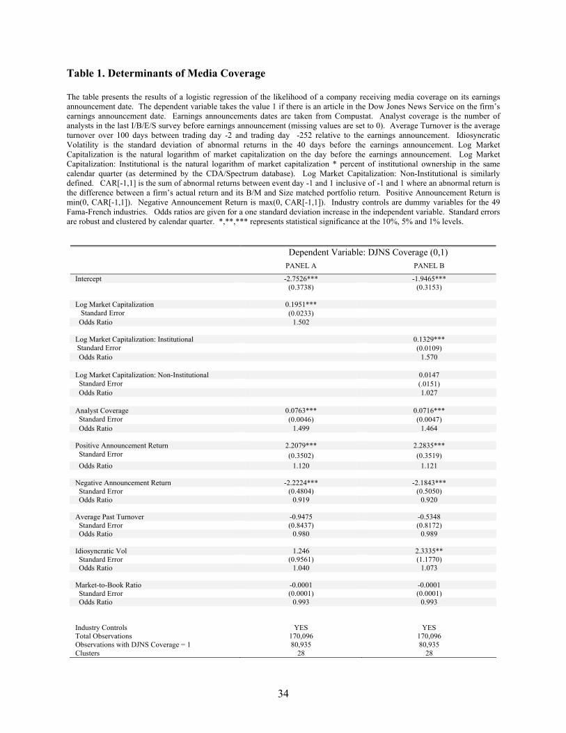
34

Table 1. Determinants of Media Coverage The table presents the results of a logistic regression of the likelihood of a company receiving media coverage on its earnings announcement date. The dependent variable takes the value 1 if there is an article in the Dow Jones News Service on the firm’s earnings announcement date. Earnings announcements dates are taken from Compustat. Analyst coverage is the number of analysts in the last I/B/E/S survey before earnings announcement (missing values are set to 0). Average Turnover is the average turnover over 100 days between trading day -2 and trading day -252 relative to the earnings announcement. Idiosyncratic Volatility is the standard deviation of abnormal returns in the 40 days before the earnings announcement. Log Market Capitalization is the natural logarithm of market capitalization on the day before the earnings announcement. Log Market Capitalization: Institutional is the natural logarithm of market capitalization * percent of institutional ownership in the same calendar quarter (as determined by the CDA/Spectrum database). Log Market Capitalization: Non-Institutional is similarly defined. CAR[-1,1] is the sum of abnormal returns between event day -1 and 1 inclusive of -1 and 1 where an abnormal return is the difference between a firm’s actual return and its B/M and Size matched portfolio return. Positive Announcement Return is min(0, CAR[-1,1]). Negative Announcement Return is max(0, CAR[-1,1]). Industry controls are dummy variables for the 49 Fama-French industries. Odds ratios are given for a one standard deviation increase in the independent variable. Standard errors are robust and clustered by calendar quarter. *,**,*** represents statistical significance at the 10%, 5% and 1% levels.

Dependent Variable: DJNS Coverage (0,1)

PANEL A PANEL B

Intercept -2.7526*** -1.9465*** (0.3738) (0.3153) Log Market Capitalization 0.1951*** Standard Error (0.0233) Odds Ratio 1.502 Log Market Capitalization: Institutional 0.1329*** Standard Error (0.0109) Odds Ratio 1.570 Log Market Capitalization: Non-Institutional 0.0147 Standard Error (.0151) Odds Ratio 1.027 Analyst Coverage 0.0763*** 0.0716*** Standard Error (0.0046) (0.0047) Odds Ratio 1.499 1.464 Positive Announcement Return 2.2079*** 2.2835*** Standard Error (0.3502) (0.3519) Odds Ratio 1.120 1.121 Negative Announcement Return -2.2224*** -2.1843*** Standard Error (0.4804) (0.5050) Odds Ratio 0.919 0.920 Average Past Turnover -0.9475 -0.5348 Standard Error (0.8437) (0.8172) Odds Ratio 0.980 0.989 Idiosyncratic Vol 1.246 2.3335** Standard Error (0.9561) (1.1770) Odds Ratio 1.040 1.073 Market-to-Book Ratio -0.0001 -0.0001 Standard Error (0.0001) (0.0001) Odds Ratio 0.993 0.993 Industry Controls YES YES Total Observations 170,096 170,096 Observations with DJNS Coverage = 1 80,935 80,935 Clusters 28 28

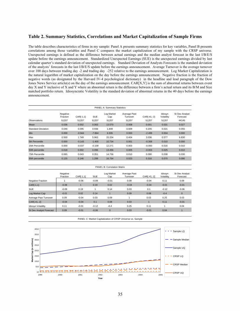
35

Table 2. Summary Statistics, Correlations and Market Capitalization of Sample Firms The table describes characteristics of firms in my sample: Panel A presents summary statistics for key variables, Panel B presents correlations among those variables and Panel C compares the market capitalization of my sample with the CRSP universe. Unexpected earnings is defined as the difference between actual earnings and the median analyst forecast in the last I/B/E/S update before the earnings announcement. Standardized Unexpected Earnings (SUE) is the unexpected earnings divided by last calendar quarter’s standard deviation of unexpected earnings. Standard Deviation of Analysts Forecasts is the standard deviation of the analysts’ forecasts in the last I/B/E/S update before the earnings announcement. Average Turnover is the average turnover over 100 days between trading day -2 and trading day -252 relative to the earnings announcement. Log Market Capitalization is the natural logarithm of market capitalization on the day before the earnings announcement. Negative fraction is the fraction of negative words (as designated by the Harvard IV-4 psychological dictionary) in the headline and lead paragraph of the Dow Jones News Service article(s) on the day of the earnings announcement. CAR[X,Y] is the sum of abnormal returns between event day X and Y inclusive of X and Y where an abnormal return is the difference between a firm’s actual return and its B/M and Size matched portfolio return. Idiosyncratic Volatility is the standard deviation of abnormal returns in the 40 days before the earnings announcement.

Negative Fraction CAR[-1,1] SUE

Log Market Cap

Average Past Turnover CAR[-41,-2]

Idiosyn Volatility

St Dev Analyst Forecast

Observations 51207 51207 51207 51207 51207 51207 51207 44145

Mean 0.036 0.002 0.063 13.570 0.008 0.001 0.031 0.027

Standard Deviation 0.046 0.095 0.936 1.849 0.009 0.205 0.021 0.055

Min 0.000 -0.944 -7.864 6.935 0.000 -2.499 0.004 0.000

Max 0.500 1.749 5.963 20.204 0.404 3.036 0.577 6.830

5th Percentile 0.000 -0.143 -1.400 10.734 0.001 -0.308 0.010 0.000

25th Percentile 0.000 -0.037 -0.109 12.271 0.003 -0.093 0.016 0.010

50th percentile 0.018 0.002 0.096 13.456 0.005 -0.003 0.025 0.010

75th Percentile 0.065 0.043 0.351 14.756 0.010 0.090 0.038 0.030

95th percentile 0.125 0.146 1.299 16.754 0.023 0.316 0.070 0.090

Negative Fraction CAR[-1,1] SUE

Log Market Cap

Average Past Turnover CAR[-41,-2]

Idiosyn Volatility

St Dev Analyst Forecast

Negative Fraction 1 -0.06 -0.09 -0.01 0.09 -0.04 0.11 0.09

CAR[-1,1] -0.06 1 0.19 0.02 -0.04 -0.04 -0.01 -0.01

SUE -0.09 0.19 1 0.14 0.03 0.1 -0.12 -0.06

Log Market Cap -0.01 0.02 0.14 1 0.09 0.08 -0.4 0

Average Past Turnover 0.09 -0.04 0.03 0.09 1 0.03 0.25 0.03

CAR[-41,-2] -0.04 -0.04 0.1 0.08 0.03 1 0.11 -0.01

Idiosyn Volatility 0.11 -0.01 -0.12 -0.4 0.25 0.11 1 0.04

St Dev Analyst Forecast 0.09 -0.01 -0.06 0 0.03 -0.01 0.04 1

PANEL B: Correlation Matrix

PANEL A: Summary Statistics

PANEL C: Market Capitalization of CRSP Universe vs. Sample

10

510

1010

1510

2010

2510

3010

3510

4010

1999 2000 2001 2002 2003 2004 2005

Year

Mar

ket C

ap (i

n m

illio

ns)

Sample LQ

Sample Median

Sample UQ

CRSP LQ

CRSP Median

CRSP UQ

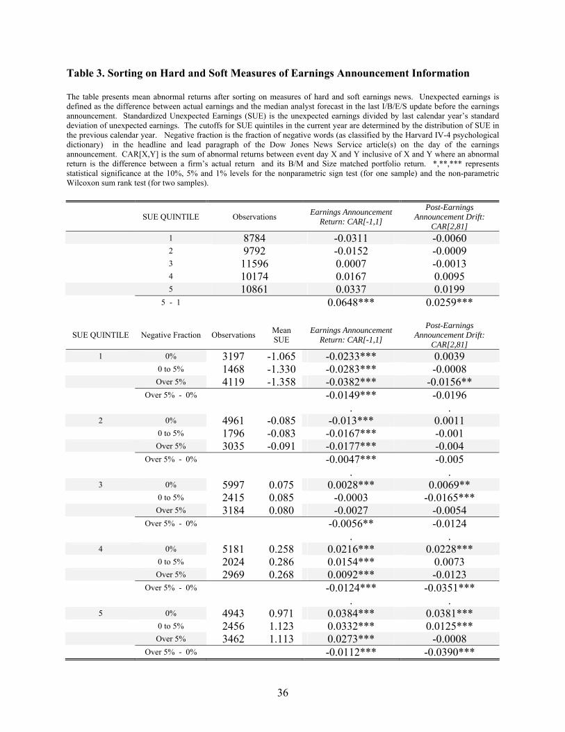
36

Table 3. Sorting on Hard and Soft Measures of Earnings Announcement Information The table presents mean abnormal returns after sorting on measures of hard and soft earnings news. Unexpected earnings is defined as the difference between actual earnings and the median analyst forecast in the last I/B/E/S update before the earnings announcement. Standardized Unexpected Earnings (SUE) is the unexpected earnings divided by last calendar year’s standard deviation of unexpected earnings. The cutoffs for SUE quintiles in the current year are determined by the distribution of SUE in the previous calendar year. Negative fraction is the fraction of negative words (as classified by the Harvard IV-4 psychological dictionary) in the headline and lead paragraph of the Dow Jones News Service article(s) on the day of the earnings announcement. CAR[X,Y] is the sum of abnormal returns between event day X and Y inclusive of X and Y where an abnormal return is the difference between a firm’s actual return and its B/M and Size matched portfolio return. *,**,*** represents statistical significance at the 10%, 5% and 1% levels for the nonparametric sign test (for one sample) and the non-parametric Wilcoxon sum rank test (for two samples).

SUE QUINTILE Observations Earnings Announcement Return: CAR[-1,1]

Post-Earnings Announcement Drift:

CAR[2,81] 1 8784 -0.0311 -0.0060 2 9792 -0.0152 -0.0009 3 11596 0.0007 -0.0013 4 10174 0.0167 0.0095 5 10861 0.0337 0.0199 5 - 1 0.0648*** 0.0259***

SUE QUINTILE Negative Fraction Observations Mean SUE

Earnings Announcement Return: CAR[-1,1]

Post-Earnings Announcement Drift:

CAR[2,81] 1 0% 3197 -1.065 -0.0233*** 0.0039 0 to 5% 1468 -1.330 -0.0283*** -0.0008 Over 5% 4119 -1.358 -0.0382*** -0.0156** Over 5% - 0% -0.0149*** -0.0196 . . 2 0% 4961 -0.085 -0.013*** 0.0011 0 to 5% 1796 -0.083 -0.0167*** -0.001 Over 5% 3035 -0.091 -0.0177*** -0.004 Over 5% - 0% -0.0047*** -0.005 . . 3 0% 5997 0.075 0.0028*** 0.0069** 0 to 5% 2415 0.085 -0.0003 -0.0165*** Over 5% 3184 0.080 -0.0027 -0.0054 Over 5% - 0% -0.0056** -0.0124 . . 4 0% 5181 0.258 0.0216*** 0.0228*** 0 to 5% 2024 0.286 0.0154*** 0.0073 Over 5% 2969 0.268 0.0092*** -0.0123 Over 5% - 0% -0.0124*** -0.0351*** . . 5 0% 4943 0.971 0.0384*** 0.0381*** 0 to 5% 2456 1.123 0.0332*** 0.0125*** Over 5% 3462 1.113 0.0273*** -0.0008 Over 5% - 0% -0.0112*** -0.0390***

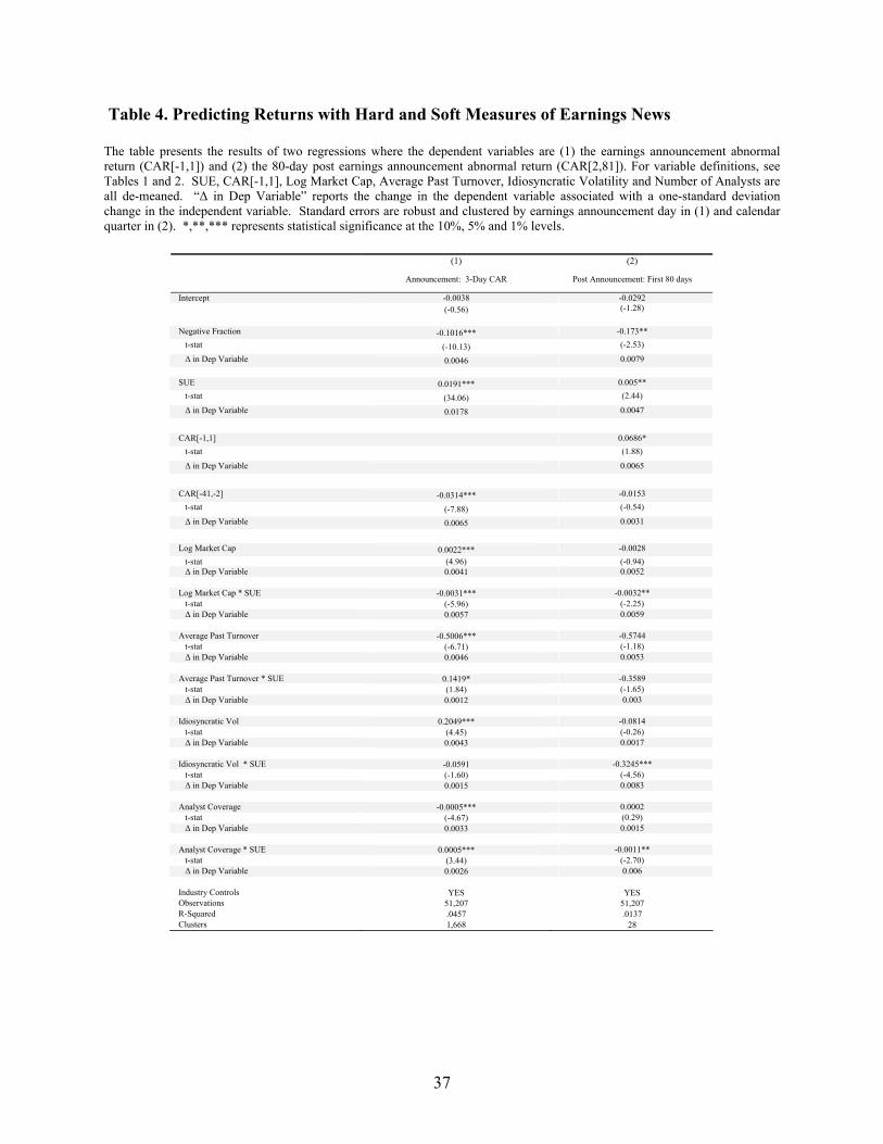
37

Table 4. Predicting Returns with Hard and Soft Measures of Earnings News The table presents the results of two regressions where the dependent variables are (1) the earnings announcement abnormal return (CAR[-1,1]) and (2) the 80-day post earnings announcement abnormal return (CAR[2,81]). For variable definitions, see Tables 1 and 2. SUE, CAR[-1,1], Log Market Cap, Average Past Turnover, Idiosyncratic Volatility and Number of Analysts are all de-meaned. “Δ in Dep Variable” reports the change in the dependent variable associated with a one-standard deviation change in the independent variable. Standard errors are robust and clustered by earnings announcement day in (1) and calendar quarter in (2). *,**,*** represents statistical significance at the 10%, 5% and 1% levels.

(1) (2)

Announcement: 3-Day CAR Post Announcement: First 80 days

Intercept -0.0038 -0.0292 (-0.56) (-1.28) Negative Fraction -0.1016*** -0.173** t-stat (-10.13) (-2.53)

Δ in Dep Variable 0.0046 0.0079 SUE 0.0191*** 0.005** t-stat (34.06) (2.44)

Δ in Dep Variable 0.0178 0.0047

CAR[-1,1] 0.0686* t-stat (1.88)

Δ in Dep Variable 0.0065

CAR[-41,-2] -0.0314*** -0.0153 t-stat (-7.88) (-0.54)

Δ in Dep Variable 0.0065 0.0031 Log Market Cap 0.0022*** -0.0028 t-stat (4.96) (-0.94) Δ in Dep Variable 0.0041 0.0052 Log Market Cap * SUE -0.0031*** -0.0032** t-stat (-5.96) (-2.25) Δ in Dep Variable 0.0057 0.0059 Average Past Turnover -0.5006*** -0.5744 t-stat (-6.71) (-1.18) Δ in Dep Variable 0.0046 0.0053 Average Past Turnover * SUE 0.1419* -0.3589 t-stat (1.84) (-1.65) Δ in Dep Variable 0.0012 0.003 Idiosyncratic Vol 0.2049*** -0.0814 t-stat (4.45) (-0.26) Δ in Dep Variable 0.0043 0.0017 Idiosyncratic Vol * SUE -0.0591 -0.3245*** t-stat (-1.60) (-4.56) Δ in Dep Variable 0.0015 0.0083 Analyst Coverage -0.0005*** 0.0002 t-stat (-4.67) (0.29) Δ in Dep Variable 0.0033 0.0015 Analyst Coverage * SUE 0.0005*** -0.0011** t-stat (3.44) (-2.70) Δ in Dep Variable 0.0026 0.006 Industry Controls YES YES Observations 51,207 51,207 R-Squared .0457 .0137 Clusters 1,668 28

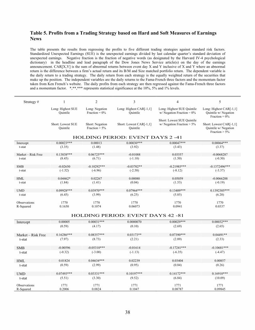
38

Table 5. Profits from a Trading Strategy based on Hard and Soft Measures of Earnings News The table presents the results from regressing the profits to five different trading strategies against standard risk factors. Standardized Unexpected Earnings (SUE) is the unexpected earnings divided by last calendar quarter’s standard deviation of unexpected earnings. Negative fraction is the fraction of negative words (as designated by the Harvard IV-4 psychological dictionary) in the headline and lead paragraph of the Dow Jones News Service article(s) on the day of the earnings announcement. CAR[X,Y] is the sum of abnormal returns between event day X and Y inclusive of X and Y where an abnormal return is the difference between a firm’s actual return and its B/M and Size matched portfolio return. The dependent variable is the daily return to a trading strategy. The daily return from each strategy is the equally weighted return of the securities that make up the position. The independent variables are the daily returns to the Fama-French three factors and the momentum factor taken from Ken French’s website. The daily profits from each strategy are then regressed against the Fama-French three factors and a momentum factor. *,**,*** represents statistical significance at the 10%, 5% and 1% levels.

Strategy # 1 2 3 4 5

Long: Highest SUE Quintile

Short: Lowest SUE Quintile

Long: Negation Fraction = 0%

Short: Negation Fraction > 5%

Long: Highest CAR[-1,1] Quintile

Short: Lowest CAR[-1,1] Quintile

Long: Highest SUE Quintile w/ Negation Fraction = 0%

Short: Lowest SUE Quintile w/ Negation Fraction > 5%

Long: Highest CAR[-1,1] Quintile w/ Negation

Fraction = 0%

Short: Lowest CAR[-1,1] Quintile w/ Negation

Fraction > 5%

HOLDING PERIOD: EVENT DAYS 2 -41 Intercept 0.00023*** 0.00013 0.00030*** 0.00047*** 0.00064*** t-stat (3.35) (1.48) (3.92) (3.43) (3.37) Market – Risk Free 0.13838*** 0.06725*** -0.01088 0.03557 -0.0068287 t-stat (8.45) (6.71) (-1.10) (1.50) (-0.30) SMB -0.02650 -0.10292*** -0.03702** -0.21985*** -0.1372496*** t-stat (-1.52) (-6.96) (-2.58) (-8.12) (-3.37) HML 0.04462* 0.02267 0.00080 0.05059 -0.0066288 t-stat (1.84) (1.41) (0.04) (1.53) (-0.19) UMD 0.09928*** 0.03970*** 0.07964*** 0.13409*** 0.1392305*** t-stat (6.45) (3.99) (6.25) (5.85) (6.20) Observations 1770 1770 1770 1770 1770 R-Squared 0.1650 0.1074 0.06073 0.0941 0.0337

HOLDING PERIOD: EVENT DAYS 42 -81

Intercept 0.00005 0.00031*** 0.0000070 0.00029*** 0.00032*** (0.59) (4.17) (0.10) (2.69) (2.65) Market – Risk Free 0.16286*** 0.08357*** 0.03173** 0.07390*** 0.04491** t-stat (7.97) (8.73) (2.21) (2.89) (2.33) SMB -0.00596 -0.05310*** -0.01614 -0.17241*** -0.10681*** t-stat (-0.32) (-3.00) (-1.13) (-6.35) (-4.47) HML 0.01824 0.04634*** 0.02239 0.03404 0.00857 t-stat (0.59) (2.99) (0.95) (0.84) (0.26) UMD 0.07493*** 0.03331*** 0.10197*** 0.14172*** 0.16910*** t-stat (5.51) (3.30) (9.52) (6.84) (10.09) Observations 1771 1771 1771 1771 1771 R-Squared 0.2006 0.0824 0.1047 0.08787 0.09845

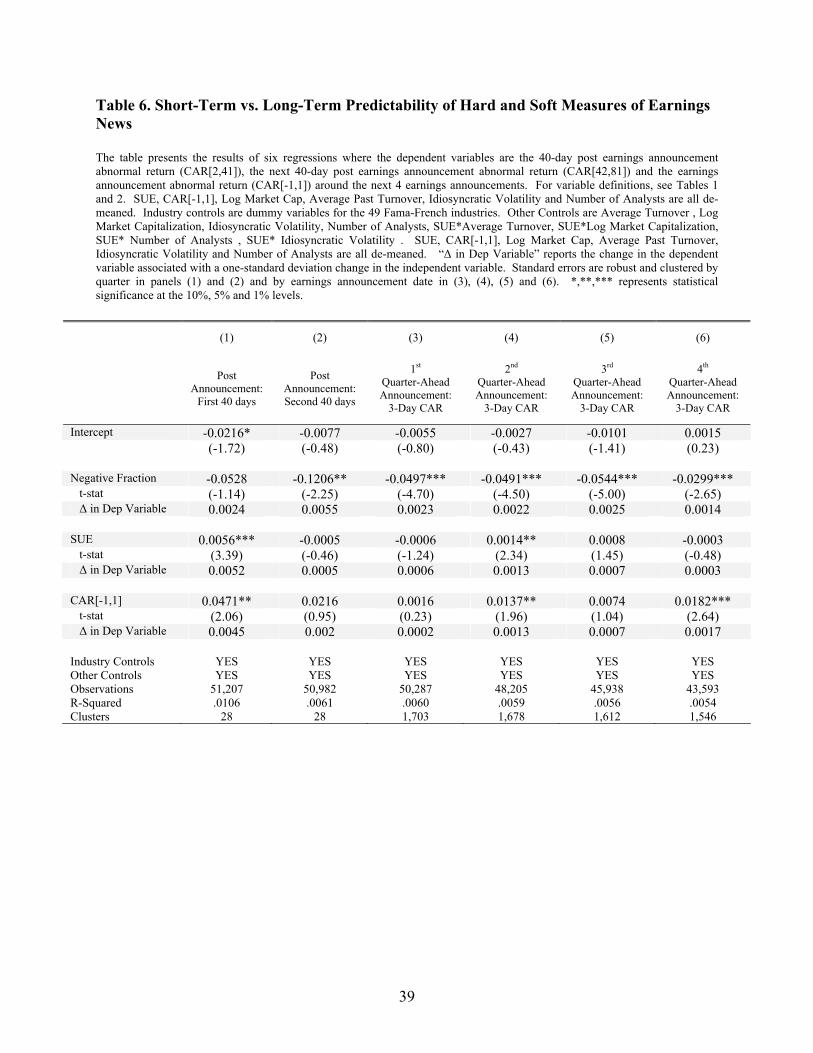
39

Table 6. Short-Term vs. Long-Term Predictability of Hard and Soft Measures of Earnings News The table presents the results of six regressions where the dependent variables are the 40-day post earnings announcement abnormal return (CAR[2,41]), the next 40-day post earnings announcement abnormal return (CAR[42,81]) and the earnings announcement abnormal return (CAR[-1,1]) around the next 4 earnings announcements. For variable definitions, see Tables 1 and 2. SUE, CAR[-1,1], Log Market Cap, Average Past Turnover, Idiosyncratic Volatility and Number of Analysts are all de-meaned. Industry controls are dummy variables for the 49 Fama-French industries. Other Controls are Average Turnover , Log Market Capitalization, Idiosyncratic Volatility, Number of Analysts, SUE*Average Turnover, SUE*Log Market Capitalization, SUE* Number of Analysts , SUE* Idiosyncratic Volatility . SUE, CAR[-1,1], Log Market Cap, Average Past Turnover, Idiosyncratic Volatility and Number of Analysts are all de-meaned. “Δ in Dep Variable” reports the change in the dependent variable associated with a one-standard deviation change in the independent variable. Standard errors are robust and clustered by quarter in panels (1) and (2) and by earnings announcement date in (3), (4), (5) and (6). *,**,*** represents statistical significance at the 10%, 5% and 1% levels.

(1) (2) (3) (4) (5) (6)

Post

Announcement: First 40 days

Post Announcement: Second 40 days

1st Quarter-Ahead Announcement:

3-Day CAR

2nd Quarter-Ahead Announcement:

3-Day CAR

3rd Quarter-Ahead Announcement:

3-Day CAR

4th Quarter-Ahead Announcement:

3-Day CAR

Intercept -0.0216* -0.0077 -0.0055 -0.0027 -0.0101 0.0015 (-1.72) (-0.48) (-0.80) (-0.43) (-1.41) (0.23) Negative Fraction -0.0528 -0.1206** -0.0497*** -0.0491*** -0.0544*** -0.0299*** t-stat (-1.14) (-2.25) (-4.70) (-4.50) (-5.00) (-2.65) Δ in Dep Variable 0.0024 0.0055 0.0023 0.0022 0.0025 0.0014 SUE 0.0056*** -0.0005 -0.0006 0.0014** 0.0008 -0.0003 t-stat (3.39) (-0.46) (-1.24) (2.34) (1.45) (-0.48) Δ in Dep Variable 0.0052 0.0005 0.0006 0.0013 0.0007 0.0003 CAR[-1,1] 0.0471** 0.0216 0.0016 0.0137** 0.0074 0.0182*** t-stat (2.06) (0.95) (0.23) (1.96) (1.04) (2.64) Δ in Dep Variable 0.0045 0.002 0.0002 0.0013 0.0007 0.0017 Industry Controls YES YES YES YES YES YES Other Controls YES YES YES YES YES YES Observations 51,207 50,982 50,287 48,205 45,938 43,593 R-Squared .0106 .0061 .0060 .0059 .0056 .0054 Clusters 28 28 1,703 1,678 1,612 1,546

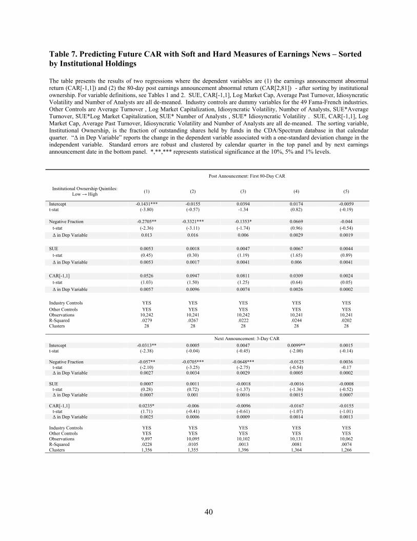
40

Table 7. Predicting Future CAR with Soft and Hard Measures of Earnings News – Sorted by Institutional Holdings The table presents the results of two regressions where the dependent variables are (1) the earnings announcement abnormal return (CAR[-1,1]) and (2) the 80-day post earnings announcement abnormal return (CAR[2,81]) - after sorting by institutional ownership. For variable definitions, see Tables 1 and 2. SUE, CAR[-1,1], Log Market Cap, Average Past Turnover, Idiosyncratic Volatility and Number of Analysts are all de-meaned. Industry controls are dummy variables for the 49 Fama-French industries. Other Controls are Average Turnover , Log Market Capitalization, Idiosyncratic Volatility, Number of Analysts, SUE*Average Turnover, SUE*Log Market Capitalization, SUE* Number of Analysts , SUE* Idiosyncratic Volatility . SUE, CAR[-1,1], Log Market Cap, Average Past Turnover, Idiosyncratic Volatility and Number of Analysts are all de-meaned. The sorting variable, Institutional Ownership, is the fraction of outstanding shares held by funds in the CDA/Spectrum database in that calendar quarter. “Δ in Dep Variable” reports the change in the dependent variable associated with a one-standard deviation change in the independent variable. Standard errors are robust and clustered by calendar quarter in the top panel and by next earnings announcement date in the bottom panel. *,**,*** represents statistical significance at the 10%, 5% and 1% levels.

Post Announcement: First 80-Day CAR

Institutional Ownership Quintiles: Low → High (1) (2) (3) (4) (5)

Intercept -0.1431*** -0.0155 0.0394 0.0174 -0.0059 t-stat (-3.80) (-0.57) -1.34 (0.82) (-0.19) Negative Fraction -0.2705** -0.3321*** -0.1353* 0.0669 -0.044 t-stat (-2.36) (-3.11) (-1.74) (0.96) (-0.54) Δ in Dep Variable 0.013 0.016 0.006 0.0029 0.0019 SUE 0.0053 0.0018 0.0047 0.0067 0.0044 t-stat (0.45) (0.30) (1.19) (1.65) (0.89) Δ in Dep Variable 0.0053 0.0017 0.0041 0.006 0.0041 CAR[-1,1] 0.0526 0.0947 0.0811 0.0309 0.0024 t-stat (1.03) (1.50) (1.25) (0.64) (0.05) Δ in Dep Variable 0.0057 0.0096 0.0074 0.0026 0.0002 Industry Controls YES YES YES YES YES Other Controls YES YES YES YES YES Observations 10,242 10,241 10,242 10,241 10,241 R-Squared .0279 .0267 .0222 .0244 .0202 Clusters 28 28 28 28 28 Next Announcement: 3-Day CAR Intercept -0.0313** 0.0005 0.0047 0.0099** 0.0015 t-stat (-2.38) (-0.04) (-0.45) (-2.00) (-0.14) Negative Fraction -0.057** -0.0705*** -0.0648*** -0.0125 0.0036 t-stat (-2.10) (-3.25) (-2.75) (-0.54) -0.17 Δ in Dep Variable 0.0027 0.0034 0.0029 0.0005 0.0002 SUE 0.0007 0.0011 -0.0018 -0.0016 -0.0008 t-stat (0.28) (0.72) (-1.37) (-1.36) (-0.52) Δ in Dep Variable 0.0007 0.001 0.0016 0.0015 0.0007 CAR[-1,1] 0.0235* -0.006 -0.0096 -0.0167 -0.0155 t-stat (1.71) (-0.41) (-0.61) (-1.07) (-1.01) Δ in Dep Variable 0.0025 0.0006 0.0009 0.0014 0.0013 Industry Controls YES YES YES YES YES Other Controls YES YES YES YES YES Observations 9,897 10,095 10,102 10,131 10,062 R-Squared .0228 .0105 .0013 .0081 .0074 Clusters 1,356 1,355 1,396 1,364 1,266

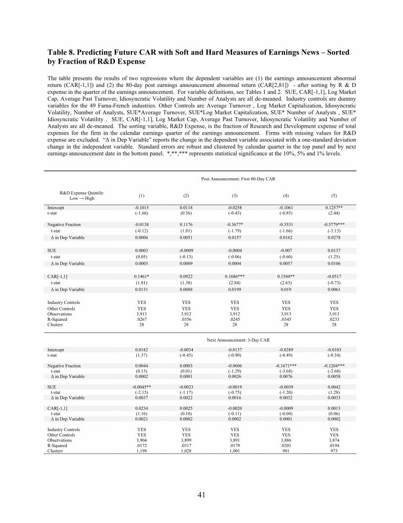
41

Table 8. Predicting Future CAR with Soft and Hard Measures of Earnings News – Sorted by Fraction of R&D Expense The table presents the results of two regressions where the dependent variables are (1) the earnings announcement abnormal return (CAR[-1,1]) and (2) the 80-day post earnings announcement abnormal return (CAR[2,81]) - after sorting by R & D expense in the quarter of the earnings announcement. For variable definitions, see Tables 1 and 2. SUE, CAR[-1,1], Log Market Cap, Average Past Turnover, Idiosyncratic Volatility and Number of Analysts are all de-meaned. Industry controls are dummy variables for the 49 Fama-French industries. Other Controls are Average Turnover , Log Market Capitalization, Idiosyncratic Volatility, Number of Analysts, SUE*Average Turnover, SUE*Log Market Capitalization, SUE* Number of Analysts , SUE* Idiosyncratic Volatility . SUE, CAR[-1,1], Log Market Cap, Average Past Turnover, Idiosyncratic Volatility and Number of Analysts are all de-meaned. The sorting variable, R&D Expense, is the fraction of Research and Development expense of total expenses for the firm in the calendar earnings quarter of the earnings announcement. Firms with missing values for R&D expense are excluded. “Δ in Dep Variable” reports the change in the dependent variable associated with a one-standard deviation change in the independent variable. Standard errors are robust and clustered by calendar quarter in the top panel and by next earnings announcement date in the bottom panel. *,**,*** represents statistical significance at the 10%, 5% and 1% levels.

Post Announcement: First 80-Day CAR

R&D Expense Quintile: Low → High (1) (2) (3) (4) (5)

Intercept -0.1015 0.0118 -0.0258 -0.1061 0.1257** t-stat (-1.66) (0.56) (-0.43) (-0.85) (2.44) Negative Fraction -0.0138 0.1176 -0.3677* -0.3531 -0.5779*** t-stat (-0.12) (1.01) (-1.79) (-1.66) (-3.13) Δ in Dep Variable 0.0006 0.0051 0.0157 0.0162 0.0278 SUE 0.0003 -0.0009 -0.0004 -0.007 0.0137 t-stat (0.05) (-0.13) (-0.06) (-0.60) (1.25) Δ in Dep Variable 0.0003 0.0009 0.0004 0.0057 0.0106 CAR[-1,1] 0.1461* 0.0922 0.1686*** 0.1544** -0.0517 t-stat (1.81) (1.38) (2.84) (2.63) (-0.73) Δ in Dep Variable 0.0131 0.0088 0.0199 0.019 0.0061 Industry Controls YES YES YES YES YES Other Controls YES YES YES YES YES Observations 3,913 3,912 3,912 3,913 3,913 R-Squared .0267 .0356 .0245 .0345 .0233 Clusters 28 28 28 28 28

Next Announcement: 3-Day CAR

Intercept 0.0182 -0.0034 -0.0137 -0.0289 -0.0103 t-stat (1.37) (-0.45) (-0.90) (-0.49) (-0.34) Negative Fraction 0.0044 0.0003 -0.0606 -0.1671*** -0.1204*** t-stat (0.13) (0.01) (-1.29) (-3.68) (-2.68) Δ in Dep Variable 0.0002 0.0001 0.0026 0.0076 0.0058 SUE -0.0045** -0.0023 -0.0019 -0.0039 0.0042 t-stat (-2.15) (-1.17) (-0.75) (-1.20) (1.28) Δ in Dep Variable 0.0037 0.0022 0.0016 0.0032 0.0033 CAR[-1,1] 0.0234 0.0025 -0.0020 -0.0009 0.0013 t-stat (1.16) (0.10) (-0.11) (-0.04) (0.06) Δ in Dep Variable 0.0021 0.0002 0.0002 0.0001 0.0002 Industry Controls YES YES YES YES YES Other Controls YES YES YES YES YES Observations 3,904 3,899 3,891 3,886 3,874 R-Squared .0172 .0317 .0179 .0201 .0194 Clusters 1,198 1,028 1,001 981 973

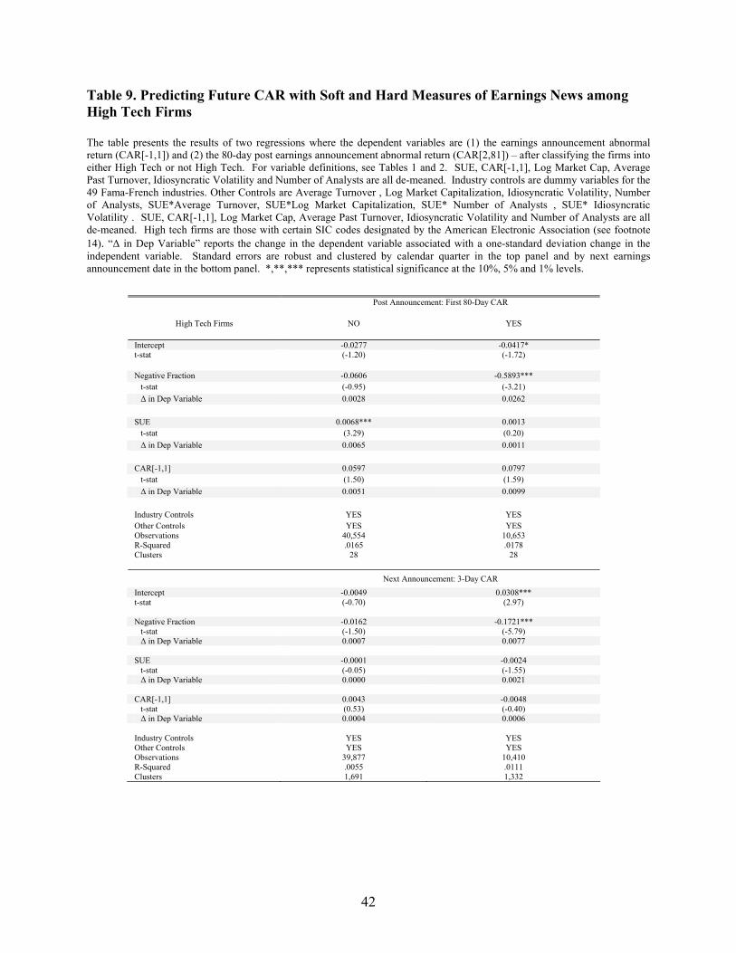
42

Table 9. Predicting Future CAR with Soft and Hard Measures of Earnings News among High Tech Firms The table presents the results of two regressions where the dependent variables are (1) the earnings announcement abnormal return (CAR[-1,1]) and (2) the 80-day post earnings announcement abnormal return (CAR[2,81]) – after classifying the firms into either High Tech or not High Tech. For variable definitions, see Tables 1 and 2. SUE, CAR[-1,1], Log Market Cap, Average Past Turnover, Idiosyncratic Volatility and Number of Analysts are all de-meaned. Industry controls are dummy variables for the 49 Fama-French industries. Other Controls are Average Turnover , Log Market Capitalization, Idiosyncratic Volatility, Number of Analysts, SUE*Average Turnover, SUE*Log Market Capitalization, SUE* Number of Analysts , SUE* Idiosyncratic Volatility . SUE, CAR[-1,1], Log Market Cap, Average Past Turnover, Idiosyncratic Volatility and Number of Analysts are all de-meaned. High tech firms are those with certain SIC codes designated by the American Electronic Association (see footnote 14). “Δ in Dep Variable” reports the change in the dependent variable associated with a one-standard deviation change in the independent variable. Standard errors are robust and clustered by calendar quarter in the top panel and by next earnings announcement date in the bottom panel. *,**,*** represents statistical significance at the 10%, 5% and 1% levels.

Post Announcement: First 80-Day CAR

High Tech Firms NO YES

Intercept -0.0277 -0.0417* t-stat (-1.20) (-1.72) Negative Fraction -0.0606 -0.5893*** t-stat (-0.95) (-3.21) Δ in Dep Variable 0.0028 0.0262 SUE 0.0068*** 0.0013 t-stat (3.29) (0.20) Δ in Dep Variable 0.0065 0.0011 CAR[-1,1] 0.0597 0.0797 t-stat (1.50) (1.59) Δ in Dep Variable 0.0051 0.0099 Industry Controls YES YES Other Controls YES YES Observations 40,554 10,653 R-Squared .0165 .0178 Clusters 28 28 Next Announcement: 3-Day CAR Intercept -0.0049 0.0308*** t-stat (-0.70) (2.97) Negative Fraction -0.0162 -0.1721*** t-stat (-1.50) (-5.79) Δ in Dep Variable 0.0007 0.0077 SUE -0.0001 -0.0024 t-stat (-0.05) (-1.55) Δ in Dep Variable 0.0000 0.0021 CAR[-1,1] 0.0043 -0.0048 t-stat (0.53) (-0.40) Δ in Dep Variable 0.0004 0.0006 Industry Controls YES YES Other Controls YES YES Observations 39,877 10,410 R-Squared .0055 .0111 Clusters 1,691 1,332

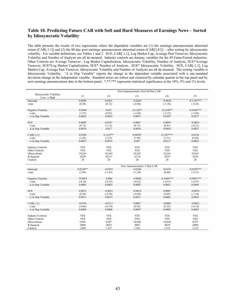
43

Table 10. Predicting Future CAR with Soft and Hard Measures of Earnings News – Sorted by Idiosyncratic Volatility The table presents the results of two regressions where the dependent variables are (1) the earnings announcement abnormal return (CAR[-1,1]) and (2) the 80-day post earnings announcement abnormal return (CAR[2,81]) - after sorting by idiosyncratic volatility. For variable definitions, see Tables 1 and 2. SUE, CAR[-1,1], Log Market Cap, Average Past Turnover, Idiosyncratic Volatility and Number of Analysts are all de-meaned. Industry controls are dummy variables for the 49 Fama-French industries. Other Controls are Average Turnover , Log Market Capitalization, Idiosyncratic Volatility, Number of Analysts, SUE*Average Turnover, SUE*Log Market Capitalization, SUE* Number of Analysts , SUE* Idiosyncratic Volatility. SUE, CAR[-1,1], Log Market Cap, Average Past Turnover, Idiosyncratic Volatility and Number of Analysts are all de-meaned. The sorting variable is Idiosyncratic Volatility. “Δ in Dep Variable” reports the change in the dependent variable associated with a one-standard deviation change in the independent variable. Standard errors are robust and clustered by calendar quarter in the top panel and by next earnings announcement date in the bottom panel. *,**,*** represents statistical significance at the 10%, 5% and 1% levels.

Post Announcement: First 80-Day CAR Idiosyncratic Volatility:

Low → High (1) (2) (3) (4) (5)

Intercept 0.0209 0.0365 -0.0269 -0.0924 -0.1162*** t-stat (0.50) (0.72) (-0.96) (-1.58) (-5.45) Negative Fraction 0.0544 0.051 -0.1225* -0.2198** -0.5444*** t-stat (1.57) (0.95) (-2.04) (-2.22) (-3.09) Δ in Dep Variable 0.0022 0.0022 0.0057 0.0107 0.0257 SUE 0.0083 0.0187 0.0041 0.0059 -0.0025 t-stat (0.72) (1.13) (0.71) (0.81) (-0.21) Δ in Dep Variable 0.0076 0.017 0.0034 0.0054 0.0027 CAR[-1,1] 0.0549 0.1107** 0.0838* 0.1307*** 0.0154 t-stat (1.29) (2.53) (1.99) (3.31) (0.28) Δ in Dep Variable 0.0027 0.0076 0.007 0.0137 0.0022 Industry Controls YES YES YES YES YES Other Controls YES YES YES YES YES Observations 10,241 10,242 10,242 10,241 10,241 R-Squared .0299 .02311 .0174 .0255 .0236 Clusters 28 28 28 28 28 Next Announcement: 3-Day CAR Intercept 0.0238** -0.0255 -0.0186 0.0124 -0.0382*** t-stat (1.99) (-1.63) (-1.28) (0.80) (-5.51) Negative Fraction -0.0024 -0.006 -0.0046 -0.1046*** -0.0981*** t-stat (-0.16) (-0.35) (-0.22) (-4.51) (-2.97) Δ in Dep Variable 0.0001 0.0003 0.0002 0.0051 0.0046 SUE 0.0012 -0.0021 -0.0014 0.0001 -0.0034 t-stat (0.28) (-0.38) (-0.50) (0.05) (-1.34) Δ in Dep Variable 0.0011 0.0019 0.0011 0.0001 0.0036 CAR[-1,1] -0.0101 -0.0111 0.0081 0.0048 -0.0022 t-stat (-0.66) (-0.74) (0.56) (0.35) (-0.18) Δ in Dep Variable 0.0005 0.0008 0.0007 0.0005 0.0003 Industry Controls YES YES YES YES YES Other Controls YES YES YES YES YES Observations 9,943 9,987 10,048 10,058 9,937 R-Squared .0090 .0033 .0087 .0070 .0090 Clusters 1,058 1,337 1,382 1,355 1,215

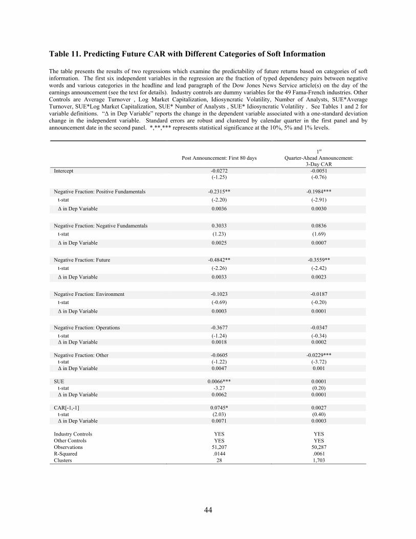
44

Table 11. Predicting Future CAR with Different Categories of Soft Information The table presents the results of two regressions which examine the predictability of future returns based on categories of soft information. The first six independent variables in the regression are the fraction of typed dependency pairs between negative words and various categories in the headline and lead paragraph of the Dow Jones News Service article(s) on the day of the earnings announcement (see the text for details). Industry controls are dummy variables for the 49 Fama-French industries. Other Controls are Average Turnover , Log Market Capitalization, Idiosyncratic Volatility, Number of Analysts, SUE*Average Turnover, SUE*Log Market Capitalization, SUE* Number of Analysts , SUE* Idiosyncratic Volatility . See Tables 1 and 2 for variable definitions. “Δ in Dep Variable” reports the change in the dependent variable associated with a one-standard deviation change in the independent variable. Standard errors are robust and clustered by calendar quarter in the first panel and by announcement date in the second panel. *,**,*** represents statistical significance at the 10%, 5% and 1% levels.

Post Announcement: First 80 days 1st

Quarter-Ahead Announcement: 3-Day CAR

Intercept -0.0272 -0.0051 (-1.25) (-0.76) Negative Fraction: Positive Fundamentals -0.2315** -0.1984*** t-stat (-2.20) (-2.91) Δ in Dep Variable 0.0036 0.0030 Negative Fraction: Negative Fundamentals 0.3033 0.0836 t-stat (1.23) (1.69) Δ in Dep Variable 0.0025 0.0007 Negative Fraction: Future -0.4842** -0.3559** t-stat (-2.26) (-2.42) Δ in Dep Variable 0.0033 0.0023 Negative Fraction: Environment -0.1023 -0.0187 t-stat (-0.69) (-0.20) Δ in Dep Variable 0.0003 0.0001 Negative Fraction: Operations -0.3677 -0.0347 t-stat (-1.24) (-0.34) Δ in Dep Variable 0.0018 0.0002 Negative Fraction: Other -0.0605 -0.0229*** t-stat (-1.22) (-3.72) Δ in Dep Variable 0.0047 0.001 SUE 0.0066*** 0.0001 t-stat -3.27 (0.20) Δ in Dep Variable 0.0062 0.0001 CAR[-1,-1] 0.0745* 0.0027 t-stat (2.03) (0.40) Δ in Dep Variable 0.0071 0.0003 Industry Controls YES YES Other Controls YES YES Observations 51,207 50,287 R-Squared .0144 .0061 Clusters 28 1,703

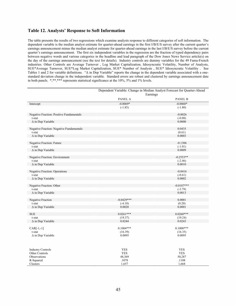
45

Table 12. Analysts’ Response to Soft Information The table presents the results of two regressions which examine analysts response to different categories of soft information. The dependent variable is the median analyst estimate for quarter-ahead earnings in the first I/B/E/S survey after the current quarter’s earnings announcement minus the median analyst estimate for quarter-ahead earnings in the last I/B/E/S survey before the current quarter’s earnings announcement. The first six independent variables in the regression are the fraction of typed dependency pairs between negative words and various categories in the headline and lead paragraph of the Dow Jones News Service article(s) on the day of the earnings announcement (see the text for details). Industry controls are dummy variables for the 49 Fama-French industries. Other Controls are Average Turnover , Log Market Capitalization, Idiosyncratic Volatility, Number of Analysts, SUE*Average Turnover, SUE*Log Market Capitalization, SUE* Number of Analysts , SUE* Idiosyncratic Volatility . See Tables 1 and 2 for variable definitions. “Δ in Dep Variable” reports the change in the dependent variable associated with a one-standard deviation change in the independent variable. Standard errors are robust and clustered by earnings announcement date in both panels. *,**,*** represents statistical significance at the 10%, 5% and 1% levels. Dependent Variable: Change in Median Analyst Forecast for Quarter-Ahead

Earnings PANEL A PANEL B Intercept -0.0069* -0.0060* (-1.85) (-1.80) Negative Fraction: Positive Fundamentals -0.0026 t-stat (-0.08) Δ in Dep Variable 0.0000 Negative Fraction: Negative Fundamentals 0.0435 t-stat (0.61) Δ in Dep Variable 0.0003 Negative Fraction: Future -0.1306 t-stat (-1.01) Δ in Dep Variable 0.0009 Negative Fraction: Environment -0.2553** t-stat (-2.46) Δ in Dep Variable 0.0010 Negative Fraction: Operations -0.0416 t-stat (-0.61) Δ in Dep Variable 0.0002 Negative Fraction: Other -0.0187*** t-stat (-3.79) Δ in Dep Variable 0.0013 Negative Fraction -0.0429*** 0.0001 t-stat (-4.10) (0.20) Δ in Dep Variable 0.0020 0.0001 SUE 0.0261*** 0.0260*** t-stat (19.37) (19.24) Δ in Dep Variable 0.0244 0.0243 CAR[-1,-1] 0.1004*** 0.1000*** t-stat (16.39) (16.35) Δ in Dep Variable 0.0095 0.0095 Industry Controls YES YES Other Controls YES YES Observations 48,369 50,287 R-Squared .1078 .1108 Clusters 1,657 1,668

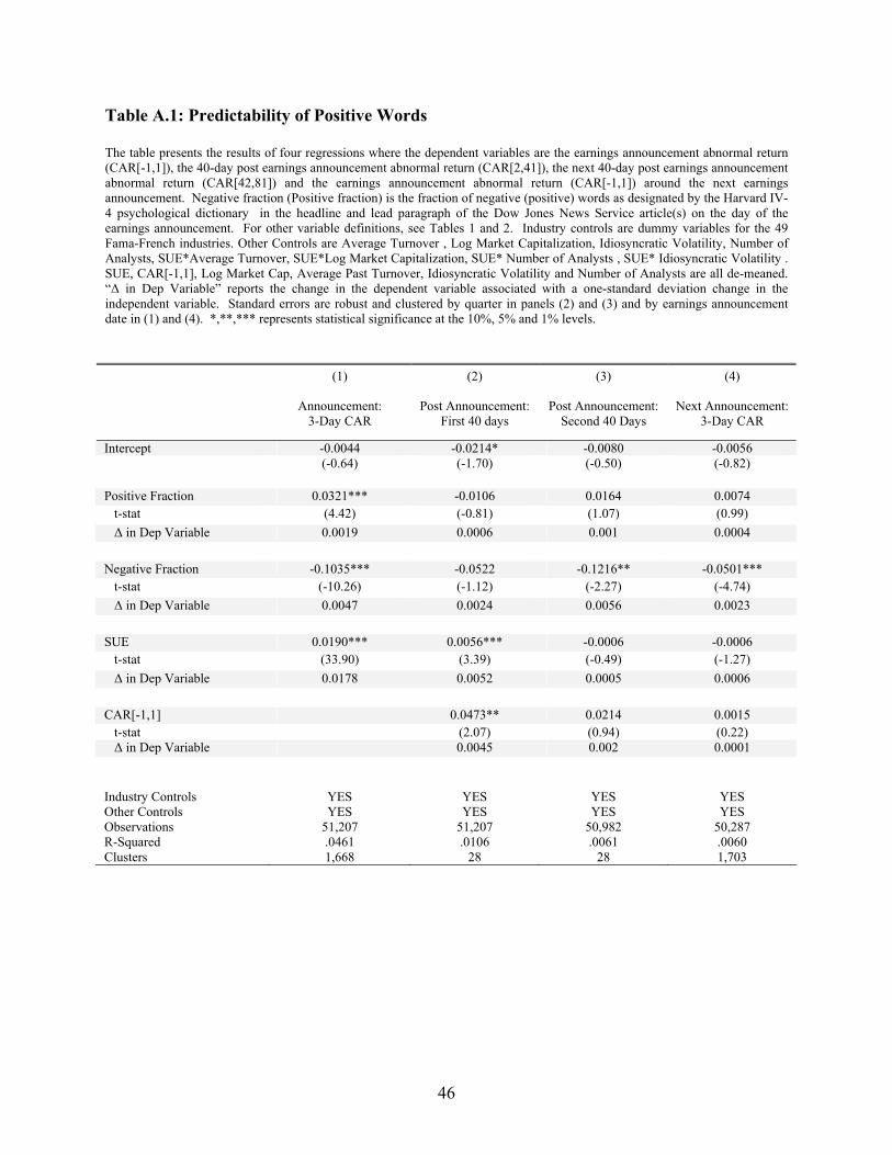
46

Table A.1: Predictability of Positive Words The table presents the results of four regressions where the dependent variables are the earnings announcement abnormal return (CAR[-1,1]), the 40-day post earnings announcement abnormal return (CAR[2,41]), the next 40-day post earnings announcement abnormal return (CAR[42,81]) and the earnings announcement abnormal return (CAR[-1,1]) around the next earnings announcement. Negative fraction (Positive fraction) is the fraction of negative (positive) words as designated by the Harvard IV-4 psychological dictionary in the headline and lead paragraph of the Dow Jones News Service article(s) on the day of the earnings announcement. For other variable definitions, see Tables 1 and 2. Industry controls are dummy variables for the 49 Fama-French industries. Other Controls are Average Turnover , Log Market Capitalization, Idiosyncratic Volatility, Number of Analysts, SUE*Average Turnover, SUE*Log Market Capitalization, SUE* Number of Analysts , SUE* Idiosyncratic Volatility . SUE, CAR[-1,1], Log Market Cap, Average Past Turnover, Idiosyncratic Volatility and Number of Analysts are all de-meaned. “Δ in Dep Variable” reports the change in the dependent variable associated with a one-standard deviation change in the independent variable. Standard errors are robust and clustered by quarter in panels (2) and (3) and by earnings announcement date in (1) and (4). *,**,*** represents statistical significance at the 10%, 5% and 1% levels. (1) (2) (3) (4)

Announcement: 3-Day CAR

Post Announcement: First 40 days

Post Announcement: Second 40 Days

Next Announcement: 3-Day CAR

Intercept -0.0044 -0.0214* -0.0080 -0.0056 (-0.64) (-1.70) (-0.50) (-0.82) Positive Fraction 0.0321*** -0.0106 0.0164 0.0074 t-stat (4.42) (-0.81) (1.07) (0.99) Δ in Dep Variable 0.0019 0.0006 0.001 0.0004 Negative Fraction -0.1035*** -0.0522 -0.1216** -0.0501*** t-stat (-10.26) (-1.12) (-2.27) (-4.74) Δ in Dep Variable 0.0047 0.0024 0.0056 0.0023 SUE 0.0190*** 0.0056*** -0.0006 -0.0006 t-stat (33.90) (3.39) (-0.49) (-1.27) Δ in Dep Variable 0.0178 0.0052 0.0005 0.0006 CAR[-1,1] 0.0473** 0.0214 0.0015 t-stat (2.07) (0.94) (0.22) Δ in Dep Variable 0.0045 0.002 0.0001 Industry Controls YES YES YES YES Other Controls YES YES YES YES Observations 51,207 51,207 50,982 50,287 R-Squared .0461 .0106 .0061 .0060 Clusters 1,668 28 28 1,703

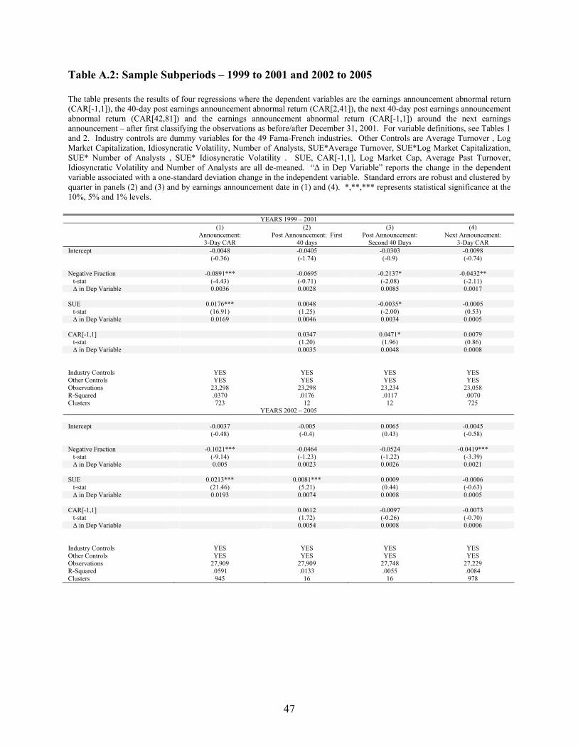
47

Table A.2: Sample Subperiods – 1999 to 2001 and 2002 to 2005 The table presents the results of four regressions where the dependent variables are the earnings announcement abnormal return (CAR[-1,1]), the 40-day post earnings announcement abnormal return (CAR[2,41]), the next 40-day post earnings announcement abnormal return (CAR[42,81]) and the earnings announcement abnormal return (CAR[-1,1]) around the next earnings announcement – after first classifying the observations as before/after December 31, 2001. For variable definitions, see Tables 1 and 2. Industry controls are dummy variables for the 49 Fama-French industries. Other Controls are Average Turnover , Log Market Capitalization, Idiosyncratic Volatility, Number of Analysts, SUE*Average Turnover, SUE*Log Market Capitalization, SUE* Number of Analysts , SUE* Idiosyncratic Volatility . SUE, CAR[-1,1], Log Market Cap, Average Past Turnover, Idiosyncratic Volatility and Number of Analysts are all de-meaned. “Δ in Dep Variable” reports the change in the dependent variable associated with a one-standard deviation change in the independent variable. Standard errors are robust and clustered by quarter in panels (2) and (3) and by earnings announcement date in (1) and (4). *,**,*** represents statistical significance at the 10%, 5% and 1% levels.

YEARS 1999 – 2001 (1) (2) (3) (4) Announcement:

3-Day CAR Post Announcement: First

40 days Post Announcement:

Second 40 Days Next Announcement:

3-Day CAR Intercept -0.0048 -0.0405 -0.0303 -0.0098 (-0.36) (-1.74) (-0.9) (-0.74) Negative Fraction -0.0891*** -0.0695 -0.2137* -0.0432** t-stat (-4.43) (-0.71) (-2.08) (-2.11) Δ in Dep Variable 0.0036 0.0028 0.0085 0.0017 SUE 0.0176*** 0.0048 -0.0035* -0.0005 t-stat (16.91) (1.25) (-2.00) (0.53) Δ in Dep Variable 0.0169 0.0046 0.0034 0.0005 CAR[-1,1] 0.0347 0.0471* 0.0079 t-stat (1.20) (1.96) (0.86) Δ in Dep Variable 0.0035 0.0048 0.0008 Industry Controls YES YES YES YES Other Controls YES YES YES YES Observations 23,298 23,298 23,234 23,058 R-Squared .0370 .0176 .0117 .0070 Clusters 723 12 12 725

YEARS 2002 – 2005 Intercept -0.0037 -0.005 0.0065 -0.0045 (-0.48) (-0.4) (0.43) (-0.58) Negative Fraction -0.1021*** -0.0464 -0.0524 -0.0419*** t-stat (-9.14) (-1.23) (-1.22) (-3.39) Δ in Dep Variable 0.005 0.0023 0.0026 0.0021 SUE 0.0213*** 0.0081*** 0.0009 -0.0006 t-stat (21.46) (5.21) (0.44) (-0.63) Δ in Dep Variable 0.0193 0.0074 0.0008 0.0005 CAR[-1,1] 0.0612 -0.0097 -0.0073 t-stat (1.72) (-0.26) (-0.70) Δ in Dep Variable 0.0054 0.0008 0.0006 Industry Controls YES YES YES YES Other Controls YES YES YES YES Observations 27,909 27,909 27,748 27,229 R-Squared .0591 .0133 .0055 .0084 Clusters 945 16 16 978

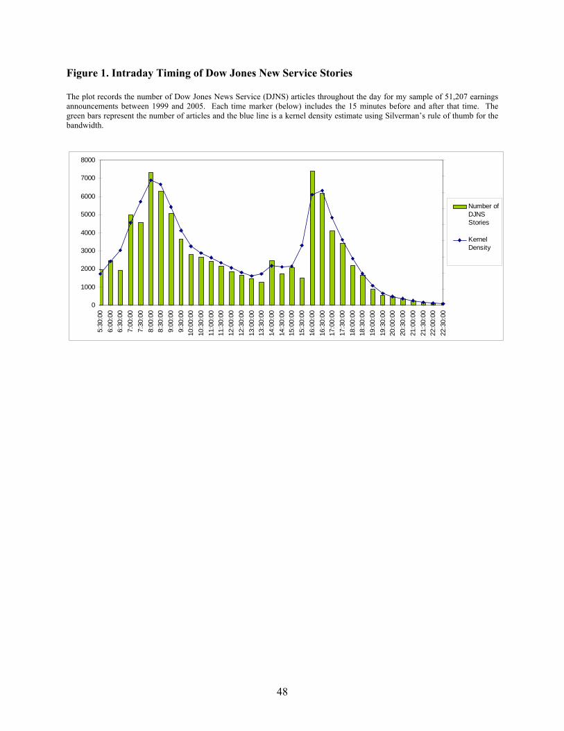
48

Figure 1. Intraday Timing of Dow Jones New Service Stories The plot records the number of Dow Jones News Service (DJNS) articles throughout the day for my sample of 51,207 earnings announcements between 1999 and 2005. Each time marker (below) includes the 15 minutes before and after that time. The green bars represent the number of articles and the blue line is a kernel density estimate using Silverman’s rule of thumb for the bandwidth.

0

1000

2000

3000

4000

5000

6000

7000

8000

5:30

:00

6:00

:00

6:30

:00

7:00

:00

7:30

:00

8:00

:00

8:30

:00

9:00

:00

9:30

:00

10:0

0:00

10:3

0:00

11:0

0:00

11:3

0:00

12:0

0:00

12:3

0:00

13:0

0:00

13:3

0:00

14:0

0:00

14:3

0:00

15:0

0:00

15:3

0:00

16:0

0:00

16:3

0:00

17:0

0:00

17:3

0:00

18:0

0:00

18:3

0:00

19:0

0:00

19:3

0:00

20:0

0:00

20:3

0:00

21:0

0:00

21:3

0:00

22:0

0:00

22:3

0:00

0.0000%

0.0005%

0.0010%

0.0015%

0.0020%

0.0025%

0.0030%

0.0035%

0.0040%

0.0045%

Number ofDJNSStories

KernelDensity

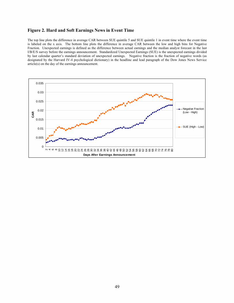
49

Figure 2. Hard and Soft Earnings News in Event Time The top line plots the difference in average CAR between SUE quintile 5 and SUE quintile 1 in event time where the event time is labeled on the x axis. The bottom line plots the difference in average CAR between the low and high bins for Negative Fraction. Unexpected earnings is defined as the difference between actual earnings and the median analyst forecast in the last I/B/E/S survey before the earnings announcement. Standardized Unexpected Earnings (SUE) is the unexpected earnings divided by last calendar quarter’s standard deviation of unexpected earnings. Negative fraction is the fraction of negative words (as designated by the Harvard IV-4 psychological dictionary) in the headline and lead paragraph of the Dow Jones News Service article(s) on the day of the earnings announcement.

0

0.005

0.01

0.015

0.02

0.025

0.03

0.035

2 4 6 8 10 12 14 16 18 20 22 24 26 28 30 32 34 36 38 40 42 44 46 48 50 52 54 56 58 60 62 64 66 68 70 72 74 76 78 80

Days After Earnings Announcement

CA

R

Negative Fraction(Low - High)

SUE (High - Low)