cooperative localization in wireless networked systems
TRANSCRIPT

University of South FloridaScholar Commons
Graduate Theses and Dissertations Graduate School
2007
Cooperative localization in wireless networkedsystemsMauricio Castillo-EffenUniversity of South Florida
Follow this and additional works at: http://scholarcommons.usf.edu/etd
Part of the American Studies Commons
This Dissertation is brought to you for free and open access by the Graduate School at Scholar Commons. It has been accepted for inclusion inGraduate Theses and Dissertations by an authorized administrator of Scholar Commons. For more information, please [email protected].
Scholar Commons CitationCastillo-Effen, Mauricio, "Cooperative localization in wireless networked systems" (2007). Graduate Theses and Dissertations.http://scholarcommons.usf.edu/etd/662

Cooperative Localization In Wireless Networked Systems
by
Mauricio Castillo-Effen
A dissertation submitted in partial fulfillment of the requirements for the degree of
Doctor of Philosophy Department of Electrical Engineering
College of Engineering University of South Florida
Co-Major Professor: Wilfrido A. Moreno, Ph.D. Co-Major Professor: Kimon P. Valavanis, Ph.D.
Miguel A. Labrador, Ph.D. James T. Leffew, Ph.D. Fernando Falquez, Ph.D.
Date of Approval: October 22, 2007
Keywords: inertial navigation, monte carlo methods, position estimation, cooperative systems, wireless networks, protocols
© Copyright 2007 , Mauricio Castillo-Effen

Dedication
“Perfection is achieved, not when there is nothing more to add, but when there
is nothing left to take away.” –Antoine de Saint-Exupéry
To each and every member of my beloved family…

Acknowledgements
I would like to express my most sincere gratitude to my two co-major professors,
Dr. Wilfrido Moreno and Dr. Kimon Valavanis. I thank them for their direction, support
and for creating the ideal research environment. The environment they have created for
their students possessed all the challenges, freedom and resources required for
completion of my research. They complemented each other perfectly.
During this research endeavor, I had the privilege of working with Dr. Miguel
Labrador. Dr. Labrador always provided important insight and guidance. In his subtle
and expert manner he showed me the beauty of academic rigor and good scientific
practices.
I also thank the other members of my committee. Dr. James Leffew and Dr.
Fernando Falquez read my documentation and provided important feedback from the
time of my research proposal until the completion of this dissertation.
I must also extend by deep appreciation to my fellow Master and Doctoral
students. With these people I worked on projects, performed experiments, wrote papers
and engaged in discussions. If it could only be true that such enjoyable pursuits will
comprise the rest of my professional life. They have all become dear friends to me.
This research was also partially supported by two grants: ARO W911NF-06-1-
0069 and SPAWAR N00039-06-C-0062.

i
Table of Contents
List of Tables vi
List of Figures vii
Abstract xi
Chapter 1 Introduction 1
1.1. Technologies on the Rise and the Emergence of Computing Paradigms 1
1.1.1. Everywhere Computing 1
1.1.2. Everything Networked 2
1.1.3. Open Spectrum 4
1.1.4. The Inertial Sensor Revolution 5
1.2. The Need for Location Information 7
1.2.1. Wireless Sensor Networks for Flash-Flood Alerting 7
1.2.2. Multi-Robot Teams With Cooperation and Coordination 11
1.3. Research Question 14
1.4. Contributions 15
1.5. Methodology 16
1.6. Document structure 17
Chapter 2 Related Work 19
2.1. A Taxonomy of Solutions for Localization 19
2.1.1. Definitions of Location 20
2.1.2. Research Communities 20
2.1.2.1. Navigation 20

ii
2.1.2.2. Robotics 21
2.1.2.3. Wireless Networking 21
2.1.2.4. Localization Theory 22
2.1.3. Categories According to Processing and Infrastructure 22
2.1.3.1. Centralized Localization 22
2.1.3.2. Infrastructure-Based Localization 23
2.1.3.3. Cooperative Localization 23
2.1.4. Sensors and Measurements 24
2.2. Salient Work 25
2.2.1. The Localization Problem from the Robotics Perspective 26
2.2.1.1. Thrun, Burgard and Fox 26
2.2.1.2. Kurazume and Nagata 26
2.2.1.3. Roumeliotis and Bekey 27
2.2.1.4. Howard, Mataric and Sukhatme 28
2.2.2. Projects in Radio-Localization 29
2.2.2.1. Active Badge and Active Office 29
2.2.2.2. Cricket 30
2.2.2.3. Radar 30
2.2.2.4. Calamari 31
2.2.2.5. Place Lab 31
2.2.3. Localization in Wireless Sensor Networks 32
2.2.4. Contributions from Inertial Navigation 33
2.2.4.1. Gustafson 33
2.2.4.2. Sukkarieh 34
2.3. Some Commercially Available Products 34
2.3.1. Northstar Robot Localization System 35
2.3.2. Liberty Latus 35
2.3.3. Vicon MX 35
2.3.4. IS900 Precision Motion Tracker 36
2.3.5. Navizon 36
2.3.6. Motorola’s Mesh Enabled Architecture 36

iii
2.4. Conclusions 37
Chapter 3 A Flexible Localization Solution 39
3.1. Definition of Localization 39
3.2. The Systems Engineering Approach 40
3.3. Requirements and Metrics 43
3.4. Structuring the Cooperative Localization Problem 48
3.4.1. Challenges and Issues in Localization 48
3.4.1.1. A Trilateration Experiment 48
3.4.1.2. Inertial Measurement Experiment 52
3.4.1.3. Summary of Challenges and Issues 55
3.4.2. Cooperative Localization and Distributed Estimation 56
3.5. Functional Analysis and Allocation 58
3.5.1. The “Localizer” – A Conceptual Solution for Cooperative Localization 60
3.5.2. Application Examples 62
3.5.2.1. A Localizer-Enabled Cell Phone 62
3.5.2.2. UAV–WSN Cooperative Localization 63
3.5.2.3. A Swarm of Ground Robots 65
3.6. The Role of Ranging 66
3.7. Summary 66
Chapter 4 Cooperative Localization in the Case of Fixed Nodes 68
4.1. Probabilistic Approach to Localization 69
4.1.1. Bayes Filter 71
4.1.1.1. Illustrating the Experiment 72
4.1.2. Particle Filters 75
4.1.3. Implementation of Resampling 79
4.2. General Assumptions 81
4.3. Varying the Number of Particles 83
4.4. Adapting Particle Filters 84
4.4.1. Tuning parameters 91

iv
4.5. Experimental Results 92
4.5.1. Experiment 1: Sensor Characterization 92
4.5.2. Experiment 2: Three Beacons and Twenty Listeners in Range 95
4.5.3. Experiment 3: Incremental Localization 97
4.6. Summary 99
Chapter 5 Localization of Mobile Nodes 101
5.1. Navigation Structure 101
5.1.1. The INS Module 104
5.1.2. The Navigation Aiding Module 105
5.1.3. The Wireless Network Interface Module 106
5.2. Assumptions 106
5.3. Probabilistic Motion Model 108
5.3.1. Preliminary Analysis of the Probabilistic Motion Model 110
5.3.2. Basic Navigation Aiding 115
5.4. Measurement Update with Respect to Non-Deterministic Reference Nodes 121
5.4.1. Gaussian Measurement: Uniform Landmark Position 123
5.4.2. Gaussian Measurement, Gaussian Reference Node Position 124
5.5. Experiments in Cooperative Localization 130
5.5.1. Cooperative Localization of Two “Passing-By” Nodes 130
5.5.2. Cooperative Localization of a Robot Swarm Moving in Formation 132
5.6. Summary 135
Chapter 6 The Role of Protocols 136
6.1. The Cricket Platform 138
6.1.1. Cricket V2.0 Protocol 138
6.1.2. The RobustLoc Application 142
6.2. Chirp Reception Frequency 143
6.3. Basic Outline of the Protocol 148
6.4. Summary 150

v
Chapter 7 Conclusions and Future Work 151
7.1. Conclusions 151
7.2. Future Work 154
References 156
About the Author End Page

vi
List of Tables
Table 1: Requirements for Localization 45
Table 2: Bayes Filter Algorithm 71
Table 3: Particle Filter Algorithm 76
Table 4: Particle Adaptation Algorithm 87
Table 5: Measurement Errors for Range Readings 94
Table 6: Quantitative Results of Experiments with the Motion Model 114
Table7: Quantitative Results of Experiments with the Motion Model and Range Measurements 120
Table 8: Experiment Conditions for two Moving and Cooperating Nodes 131
Table 9: Experimental Results Showing the Effect of Cooperation and no Cooperation for a Mobile Node 132
Table 10: Experimental Conditions for Localization of a Robot Swarm 133
Table 11: Results of Cooperative Localization in a Robot Swarm 134

vii
List of Figures
Figure 1: Ubiquitous Computing Example 2
Figure 2: A Wireless Sensor Node for Flash-flood Alerting 3
Figure 3: Conceptual SDR Platform 5
Figure 4: Analog Devices’ ADIS16350 Block Diagram 6
Figure 5: Flash-Flood Prone Zone in Venezuela 8
Figure 6: Wireless Sensor Network-Based Flash-Flood Alert System 10
Figure 7: Robots and Sensors for Cooperative Exploration of Occluded Spaces 14
Figure 8: Block Diagram of a GNC System 42
Figure 9: Setup for a Trilateration Experiment 49
Figure 10: Results of a Trilateration Experiment 50
Figure 11: The Microstrain’s 3DM-GX1 Inertial Measurement Unit 52
Figure 12: Measured Acceleration with Basic Statistical Parameters 53
Figure13: Measured Angular Rate with Basic Statistical Parameters 53
Figure 14: “Virtual” Motion of a Static Object Due to Errors 54
Figure 15: Three Aspects of Cooperative Localization 56
Figure16: Cooperative Estimation 58
Figure 17: Main Functions of the Cooperative Estimation Solution 58
Figure 18: Simplified Representation of the “Localizer” 61
Figure 19: A Localizer-Enabled Cell Phone for Pedestrian Navigation 63
viii
Figure 20: UAV-WSN Cooperative Localization 64
Figure 21: A Swarm of Ground Robots Equipped with Localizers 65
Figure 22: Localization as a Hidden Markov Model 70
Figure 23: Configuration of Beacons and a Listener 72
Figure 24: Belief after one Range Measurement 73
Figure 25: Belief after two Range Measurements 73
Figure 26: Belief after three Range Measurements 74
Figure 27: Particle Filter Initialization 77
Figure 28: Particles after the First Range Measurement 77
Figure 29: Particles after a Second Range Measurement 78
Figure 30: Particles after a Third Range Measurement 78
Figure 31: Set of Uniformly Distributed Particles and Their Histogram 79
Figure 32: Weighted Particles 80
Figure 33: Cumulative Weight of Weighted Particles 80
Figure 34: Resampled Set of Particles with Corresponding Histogram 81
Figure 35: Convergence as a Function of Particle Size 83
Figure 36: Particle Updating 86
Figure 37: Measurement Distributions 93
Figure 38: Position of the COGs of Particles after 12 Chirps, (1 unit ≡ 0.3m) 96
Figure 39: Convergence of the Average Position Error 97
Figure 40: Incremental Localization Experiment: Estimates after 100 Chirps, (1 unit ≡ 0.3m) 98
Figure 41: Convergence of Position Error in Incremental Localization 99
Figure 42: A Common GPS/INS Integration Topology 102
ix
Figure 43: Proposed Structure for Aided Navigation 103
Figure 44: PMM for 1m sv = / and 0rad sω = / 111
Figure 45: PMM for 1m sv = / and 0 05rad sω = . / 112
Figure 46: PMM for 1m sv = / and [0 1( 10) ( 0 1)( 10)]rad st tω = . < + − . ≥ / 112
Figure 47: PMM with Greater Uncertainty in v : 1 2 0 5α , = . , 3 4 5 6 0 05α , , , = . 113
Figure 48: PMM with Greater Uncertainty inω : 3 4 0 5α , = . , 1 2 5 6 0 05α , , , = . 113
Figure 49: PMM with Greater Uncertainty in γ : 5 6 0 5α , = . , 1 2 3 4 0 05α , , , = . 114
Figure 50: Measurement Probability, ( )t tp z x| 116
Figure 51: PMM for 1m sv = / and 0rad sω = / with Measurement Updates 117
Figure 52: PMM for 1m sv = / and 0 05rad sω = . / with Measurement Updates 117
Figure 53: PMM for 1m sv = / and Varying ω with Measurement Updates 118
Figure 54: PMM with Greater Uncertainty in v With Measurement Updates 118
Figure 55: PMM with Greater Uncertainty in ω with Measurement Updates 119
Figure 56: PMM with Greater Uncertainty in γ with Measurement Updates 119
Figure 57: Combination of Measurement Distributions with Position Belief 124
Figure 58: Position Belief of the Reference Node 128
Figure 59: PDF of the Range Measurement 128
Figure 60: PDF of the Range Measurement Obtained from Convolution 129
Figure 61: Belief after Applying a Measurement Update with a Convolved PDF 130
Figure 62: Two “Passing-by” Nodes 1m sv = / and 0rad sω = / 131
Figure 63: Robots moving in a Square-Shaped Formation 132
Figure 64: Cooperative Localization in a Robot Swarm 134

x
Figure 65: The Two Lower Layers of the OSI Model 137
Figure 66: Cricket V2.0 Configuration 140
Figure 67: Cricket V2.0 Protocols 142
Figure 68: RobustLoc Protocol 143
Figure 69: Histograms for the Inter-Arrival Time from Six Nodes 146
Figure 70: Probability of, n , Chirps Received; { (1 ) }P N s n= 147
Figure 71: Basic Localization Protocol for a WSN 150
xi
Localization in Wireless Networked Systems
Mauricio Castillo Effen
Abstract
A novel solution for the localization of wireless networked systems is presented.
The solution is based on cooperative estimation, inter-node ranging and strap-down
inertial navigation. This approach overrides limitations that are commonly found in
currently available localization/positioning solutions. Some solutions, such as GPS,
make use of previously deployed infrastructure. In other methods, computations are
performed in a central fusion center. In the robotics field, current localization techniques
rely on a simultaneous localization and mapping, (SLAM), process, which is slow and
requires sensors such as laser range finders or cameras.
One of the main attributes of this research is the holistic view of the problem and
a systems-engineering approach, which begins with analyzing requirements and
establishing metrics for localization. The all encompassing approach provides for
concurrent consideration and integration of several aspects of the localization problem,
from sensor fusion algorithms for position estimation to the communication protocols
required for enabling cooperative localization. As a result, a conceptual solution is
presented, which is flexible, general and one that can be adapted to a variety of
application scenarios. A major advantage of the solution resides in the utilization of
wireless network interfaces for communications and for exteroceptive sensing. In

xii
addition, the localization solution can be seamlessly integrated into other localization
schemes, which will provide faster convergence, higher accuracy and less latency.
Two case-studies for developing the main aspects of cooperative localization were
employed. Wireless sensor networks and multi-robot systems, composed of ground
robots, provided an information base from which this research was launched. In the
wireless sensor network field, novel nonlinear cooperative estimation algorithms are
proposed for sequential position estimation. In the field of multi-robot systems the issues
of mobility and proprioception, which uses inertial measurement systems for estimating
motion, are contemplated. Motion information, in conjunction with range information
and communications, can be used for accurate localization and tracking of mobile nodes.
A novel partitioning of the sensor fusion problem is presented, which combines an
extended Kalman filter for dead-reckoning and particle filters for aiding navigation.

1
Chapter 1
Introduction
1.1. Technologies on the Rise and the Emergence of Computing Paradigms
Cooperative localization, as presented in this dissertation, lies at the heart of the
rise of technological advances, which are poised to change the day-to-day life of the
world’s societies. In order to allow for the reader to place this research in its proper
context, the current technological developments, which motivate and enable the practical
realization of the ideas and concepts presented, are summarized.
1.1.1. Everywhere Computing
As in the realm of Mark Weiser’s vision of “Ubiquitous Computing”, currently,
people come into contact with objects that incorporate embedded processors, without
giving any consideration to how things work internally, [1]. Advances in semiconductor
fabrication capabilities provide the verification that Moore’s law still holds. Larger
computing power, larger memory capacity in ever-shrinking electronic packaging and
reduction of prices are reported daily. Inevitably, the pervasiveness of these devices will
provide for the creation of, so called, smart or situation-aware environments, [2]. Smart
environments work on behalf of humans. The attempt to serve their occupants needs and
fulfill their expressed desires. In addition, smart environments are conceived, which will
attempt to deduce their occupants desires and requirements. Embedded computers may

2
someday become a part of a person’s physical makeup. Currently, computers, which are
veiled in clothing, are available to be carried by people. Such capability has, in the last
few years, been extensively researched in the wearable computing field, [3]. Figure 1,
presents an experimental office environment with, what the authors term, “roomware”
components, [4].
Figure 1: Ubiquitous Computing Example:
Streitz et al., 2005, [4]
Roomware components such as computers and their interfaces form part of the
walls and furniture and provide interactive collaboration tools. The ultimate goal consists
in having people not perceive of computers as such. Rather, people, while performing
their activities, will interact intuitively with their computational assistants to produce
more efficient and error free activities.
1.1.2. Everything Networked
Developments do not stop at everywhere computing. The latest communications
and networking technologies have enabled embedded systems to communicate among
3
each other and to connect to and through the largest interconnected system in the world,
the Internet. The communications modality with the fastest pace of growth is wireless
with its key thrust stemming from personal communications. Aside from the rather
trivial personal communications applications, it is widely accepted that, in a not so distant
future, hordes of tiny and low-cost sensors will be pervasively installed for collecting
data related to physical quantities of every imaginable kind [5]. This development has
already started, [6]. The usefulness of the, so called, Wireless Sensor Networks, (WSNs),
has been studied extensively presented and in several publications. For instance, WSNs
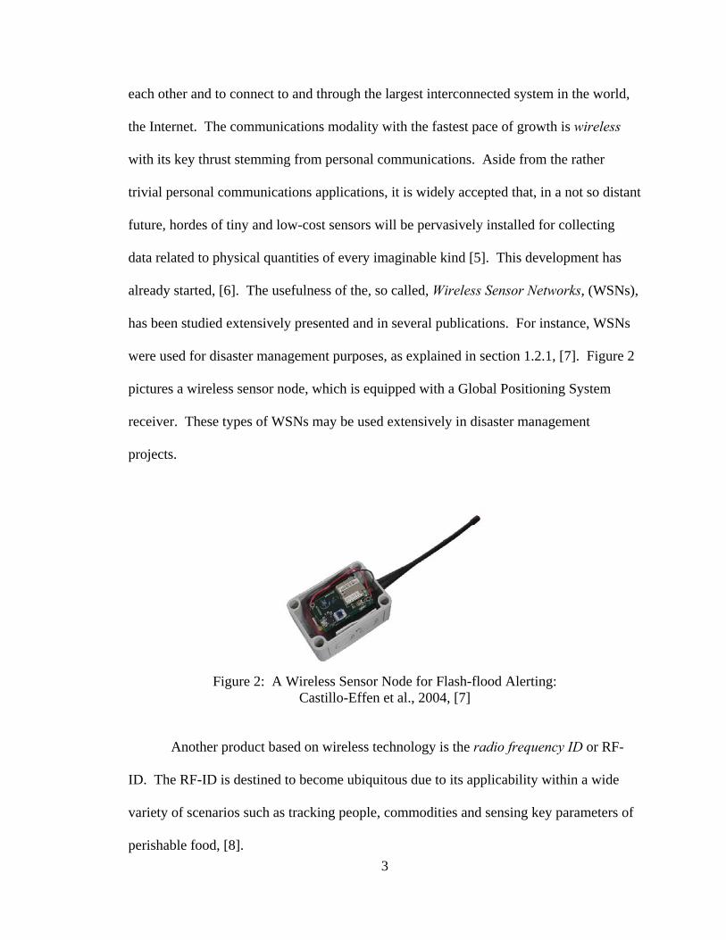
were used for disaster management purposes, as explained in section 1.2.1, [7]. Figure 2
pictures a wireless sensor node, which is equipped with a Global Positioning System
receiver. These types of WSNs may be used extensively in disaster management
projects.
Figure 2: A Wireless Sensor Node for Flash-flood Alerting:
Castillo-Effen et al., 2004, [7]
Another product based on wireless technology is the radio frequency ID or RF-
ID. The RF-ID is destined to become ubiquitous due to its applicability within a wide
variety of scenarios such as tracking people, commodities and sensing key parameters of
perishable food, [8].

4
While technical issues with respect to spectrum band allocation are being
resolved, it seems that the, so-called, Fixed to Mobile Convergence, (FMC), and the
Mobile to Mobile Convergence, (MMC), are imminent, [9]. As a result, these
technologies will provide for a high degree of integration of cell phones into corporate
fixed line telecommunications/networking infrastructures. These infrastructures will
allow services to be provided to users regardless of location, the terminals, physical radio
technology or protocols they may employ.
1.1.3. Open Spectrum
The constant growth of users of wireless communication devices has generated a
congested and inadequately utilized electromagnetic spectrum, which is considered by
many as a “precious natural resource” [10]. This development has generated a
completely new approach to the use of the radiofrequency spectrum. Ideally, this new
approach should fulfill some basic requirements such as, [10]:
• Provide highly reliable communication channels between users,
• Use the electromagnetic frequency spectrum efficiently,
• Do not interfere with communications of frequency bands licensed to
primary users.
Undoubtedly, the achievement of these goals can only be obtained if communication
devices have a degree of “intelligence” and if they are aware of the presence of other
communication parties by sensing the event of instantaneous spectrum occupation.
These concepts have been summarized and well documented under the definition
of cognitive radio [11]. The key enabler, at the core of cognitive radio, is a highly

5
flexible platform, which is known as Software Defined Radio, (SDR). Conceptually,
SDR is nothing more than a digital signal processing device. Together with a wideband
receiving and transmitting front-end and wideband signal converters, the SDR processes
signals at the baseband. Figure 3 depicts this conceptual platform.
Figure 3: Conceptual SDR Platform
Developments in reconfigurable computing indicate that the best way to perform signal
processing within the SDR platform may be based on programmable hardware such as
Field-Programmable Gate Arrays, (FPGAs). Reconfigurable computing will make the
basic objectives of cognitive radio possible. In addition, reconfigurable computing opens
up new possibilities of having full interoperability among devices equipped with wireless
communications interfaces. These capabilities are currently being tested in the Joint
Tactical Radio System, (JTRS), military research program, [12]. These efforts are
important steps towards the “everything networked” future.
1.1.4. The Inertial Sensor Revolution
The MEMS, (Micro Electro-Mechanical Systems), revolution has engendered a
wide variety of devices aimed at sensing motion in all things that move. Inertial sensors
is the term applied to these motion sensors. These devices have experienced a drop in
their cost. Therefore, they are used more and more in everyday life. The price drop has
6
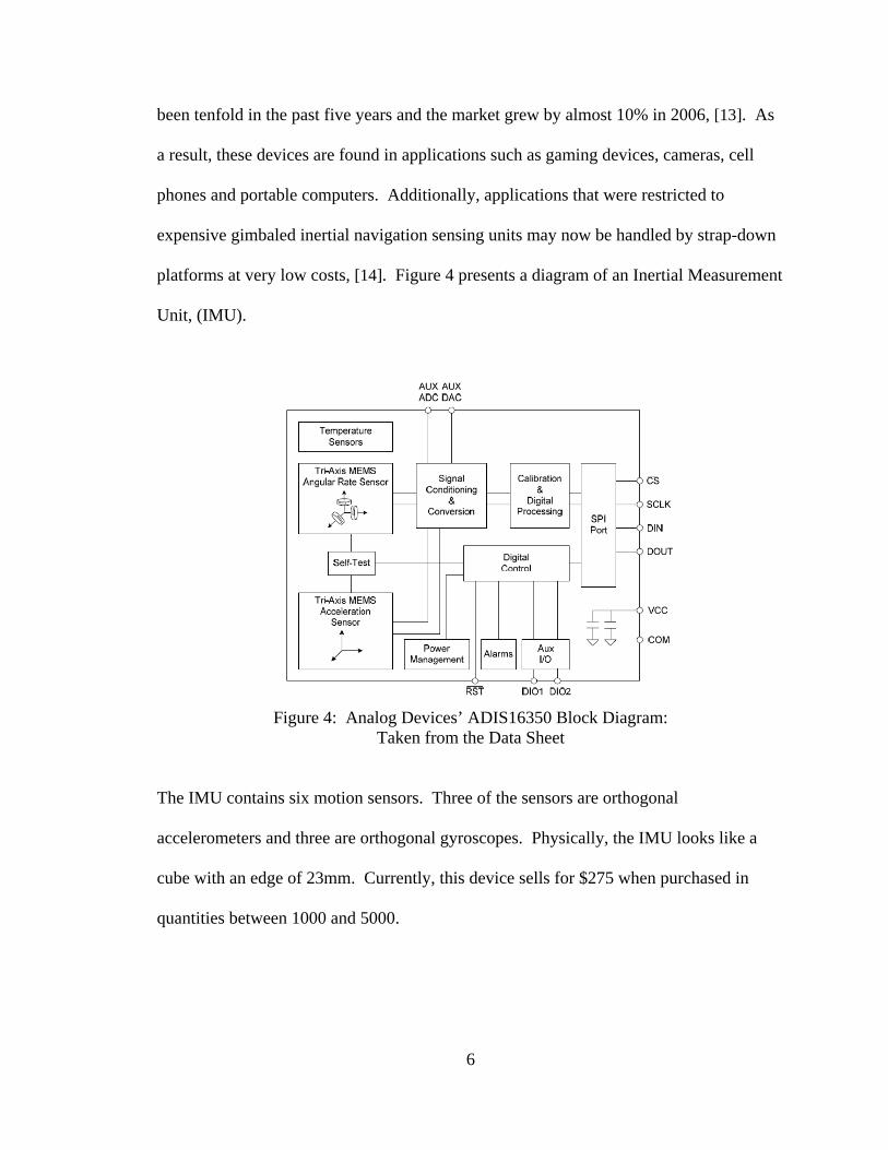
been tenfold in the past five years and the market grew by almost 10% in 2006, [13]. As
a result, these devices are found in applications such as gaming devices, cameras, cell
phones and portable computers. Additionally, applications that were restricted to
expensive gimbaled inertial navigation sensing units may now be handled by strap-down
platforms at very low costs, [14]. Figure 4 presents a diagram of an Inertial Measurement
Unit, (IMU).
Figure 4: Analog Devices’ ADIS16350 Block Diagram:
Taken from the Data Sheet
The IMU contains six motion sensors. Three of the sensors are orthogonal
accelerometers and three are orthogonal gyroscopes. Physically, the IMU looks like a
cube with an edge of 23mm. Currently, this device sells for $275 when purchased in
quantities between 1000 and 5000.
7
1.2. The Need for Location Information
The possibility exists of having mobile computing devices, which build wireless
networks spontaneously or in an ad-hoc manner. Such a possibility has generated a
multiplicity of potential applications. Furthermore, “location-awareness” is supposed to
become mainstream as part of the pervasive computing revolution [15]. Location aware
computing encompasses applications such as everyday office productivity, personal
navigation, emergency preparedness and intelligent transportation systems.
Two research projects, where localization plays a crucial role, are presented next.
They are introduced to highlight the need for real-time location information. Such data is
crucial in applications where devices incorporate wireless networking interfaces. These
projects, wherein this author was actively involved, served also as motivation for
pursuing this research.
1.2.1. Wireless Sensor Networks for Flash-Flood Alerting
The primary purpose of the Rapid Organization and Situation Assessment project
was to aid the population of the Andean region of Venezuela. Specifically, the city of
Merida and its neighboring towns were chosen as the area for development of an Early
Alert System based on a WSN. Large amounts of property damage and resident
casualties caused by flash-floods were reported over the years. Additionally,
hydrological and geological studies had shown that the region was highly prone to similar
events in near future.
A flash-flood is a sudden discharge of large amounts of water. It results from a
particular confluence and chain of meteorological and geological events. The mountains

8
that surround the borders of the rivers have geologically unstable characteristics. In the
event of high precipitation levels, some zones of the mountains provide origin to
landslides that fall into the rivers, which occludes the flow of water. Eventually, these
naturally built barriers cannot sustain the high potential energy of the accumulated water.
When the barriers finally break, a rush of water occurs, which affects the villages
downstream. This chain of events happens in a short period of time, (few hours), which
poses a serious challenge for authorities who try to protect the population. Figure 5
pictures a set of houses, which are prone to be wiped out by the interaction between the
mountains and the rivers in the formation of a flash-flood.
Figure 5: Flash-Flood Prone Zone in Venezuela:
Matthew C. Larsen, USGS
The solution to this problem involves the application of several communication
and information technologies. The flash-flood alert system is presented in Figure 6.
Basically, the alert system consists of three major components:
• A WSN for collecting information in the places where variables need to be
measured. The self-healing/self-forming multi-hopping nature of a WSN

9
allows for a robust low-cost sensing solution that can be deployed swiftly and
easily. The main variables to be measured are:
• Soil humidity, for detecting landslides,
• Precipitation, (rainfall),
• Water level sensors, situated in strategic locations of the rivers,
• Other meteorological sensors, such as wind speed, temperature, sun
radiation and barometric pressure, for disaster prediction.
• A sink node, located close to the sensor network whose function is collecting
data from the wireless sensor nodes. Periodically, or in case of abnormal
conditions, the sink sends information via cellular network to a central
location.
• A central location or command center. At the command center, emergency
preparedness authorities make decisions with the help of a computer system.
The computer system collects data and augments a Geographical Information
System, (GIS), with a layer of live data incoming from the distant WSN.

10
Figure 6: Wireless Sensor Network-Based Flash-Flood Alert System
It is critical that the location of the nodes be known with good accuracy for
achieving a successful overlay of sensor data with the GIS maps. As a consequence, the
decision makers have access to relevant information in order to take appropriate
mitigation measures. In some cases, sensors nodes are located in places with Line of
Sight, (LOS), access to GPS satellites. Therefore, they can determine their location with
little error and almost no effort. However, there are places where mountains or
vegetation obstruct the direct LOS between sensor nodes and some of the GPS satellites.
These conditions cause a loss of fix condition, which prevents the nodes from determining
their location.
The research, presented in this dissertation, was directed towards providing means
for localization in a distributed fashion, without the requirement of having GPS receivers
in all the nodes. In wireless sensor networks, “strength is in numbers”. Sensors are
deployed in large quantities. Therefore, they need to be low in cost. Having a GPS

11
receiver in every unit would increase the cost of the system unnecessarily. Ideally, nodes
with GPS receivers should cooperate with nodes that do not possess GPS receivers. After
some time and through several information exchanges, all nodes will have good position
estimates.
Location information is essential for the usefulness of the data provided by the
nodes. Location information is also important for implementing important algorithms for
network management. Network management algorithms such as power management,
node addressing and the implementation of efficient location aware routing protocols
may be simplified to a great extent using location information. Solutions to these types
of localization requirements are explored initially in Chapter 3. Afterwards, localization
in sensor networks is expounded in Chapter 4.
1.2.2. Multi-Robot Teams With Cooperation and Coordination
The ability of a robot to localize itself is an essential prerequisite for autonomy.
For this reason, localization is also regarded as the most basic perceptual problem in
robotics, [16]. A robot needs to estimate its current position in order to determine the
next action. The position estimate with respect to local features determines the
immediate actions performed by the robot. On the other hand, the position with respect
to some semi-global coordinate system helps the robot establish the actions to take within
a longer time-horizon or broader scope, such as part of a plan or mission within a team.
For multi-robot teams, relative location with respect to other members of the team is
fundamental for achieving coordination and cooperation during such activities as
formation control, swarming, cooperative search and exploration. Localization in a
12
multi-robot system is fundamental for exploiting redundancy and complementarities
inherent to a system composed of multiple heterogeneous individuals. When ground
robots navigate in an unknown environment, it has been shown that it is advantageous to
perform the action in a specific formation [17]. Different formations adapt to particular
goals such as exploration and surveillance. In addition, formations can help in keeping a
required node degree in a network topology. Moreover, if every robot is aware of its
location, resource sharing and task allocation can be enacted more efficiently. Some
mechanisms for task allocation, such as auction-based methods, have been reported
extensively in the current literature [18].
One major contribution of this research consists in enabling localization in
scenarios where multi-robot systems have to be deployed in an ad-hoc manner and
execute missions with minimal human intervention. Chiefly, occluded and unstructured
environments where no prior knowledge is easily accessible, such as maps, pose a great
challenge to currently used localization schemes. For example, GPS-based solutions do
not work in environments surrounded by objects that intermittently block the line of sight
to GPS-satellites. As a consequence, equipping each robot or sensor node with a GPS-
receiver does not assure correct positioning in all situations and/or at all times.
Simultaneous Localization and Mapping, (SLAM), techniques studied profusely
in current literature are known to give good results in structured environments such as the
indoors, [16]. SLAM techniques assume the availability of relatively accurate
exteroceptive sensing such as the one obtained from laser range-finders. At the same
time, the proposed solutions usually make extensive use of computational resources
onboard the robots. It will be shown in Chapter 5, that there are not many solutions,
13
reported in the literature, that make use of SLAM techniques in multi-robot systems in
the context of unstructured outdoor locations. Moreover, in such applications, a map is
an outcome of the relatively slow SLAM process. In many cases, a map is neither needed
nor required within the scope of a mission with severe time constraints.
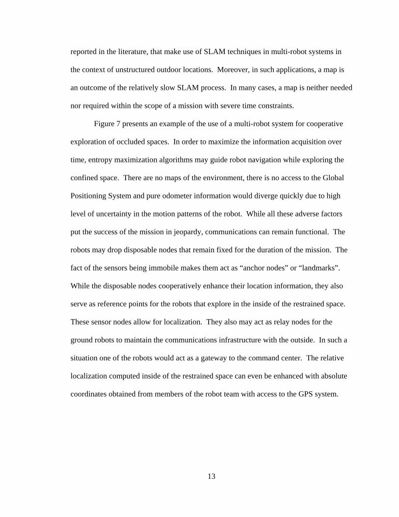
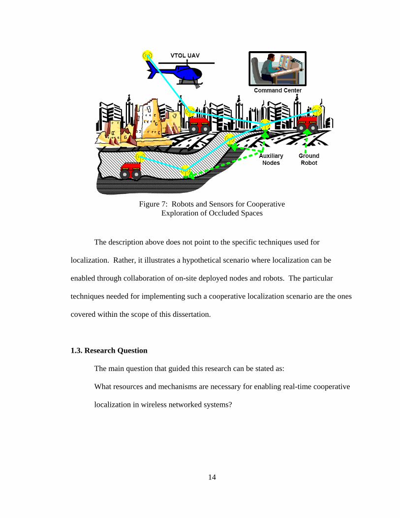
Figure 7 presents an example of the use of a multi-robot system for cooperative
exploration of occluded spaces. In order to maximize the information acquisition over
time, entropy maximization algorithms may guide robot navigation while exploring the
confined space. There are no maps of the environment, there is no access to the Global
Positioning System and pure odometer information would diverge quickly due to high
level of uncertainty in the motion patterns of the robot. While all these adverse factors
put the success of the mission in jeopardy, communications can remain functional. The
robots may drop disposable nodes that remain fixed for the duration of the mission. The
fact of the sensors being immobile makes them act as “anchor nodes” or “landmarks”.
While the disposable nodes cooperatively enhance their location information, they also
serve as reference points for the robots that explore in the inside of the restrained space.
These sensor nodes allow for localization. They also may act as relay nodes for the
ground robots to maintain the communications infrastructure with the outside. In such a
situation one of the robots would act as a gateway to the command center. The relative
localization computed inside of the restrained space can even be enhanced with absolute
coordinates obtained from members of the robot team with access to the GPS system.
14
Figure 7: Robots and Sensors for Cooperative
Exploration of Occluded Spaces
The description above does not point to the specific techniques used for
localization. Rather, it illustrates a hypothetical scenario where localization can be
enabled through collaboration of on-site deployed nodes and robots. The particular
techniques needed for implementing such a cooperative localization scenario are the ones
covered within the scope of this dissertation.
1.3. Research Question
The main question that guided this research can be stated as:
What resources and mechanisms are necessary for enabling real-time cooperative
localization in wireless networked systems?
15
1.4. Contributions
The main contributions of this research are:
• A novel flexible solution to localization, which is based on distributed
cooperative localization. This approach unifies networking and inertial
navigation in a way that has neither been reported elsewhere in the current
literature nor implemented in commercial solutions.
• Structuring of the cooperative localization problem. A systems-
engineering analysis of the main localization function with allocated sub-
functions is presented.
• Simple cooperative nonlinear distributed estimation laws were developed,
which are amenable for localization of devices with constraints in
computational resources and power, such as Wireless Sensor Nodes. Most
standard approaches resource on optimal estimation techniques. However,
they do not suggest simple suboptimal nonlinear estimation laws for
WSNs such as the ones described in this document.
• Data fusion algorithms were developed to enable cooperative localization
of wireless networked systems with mobile nodes. A concrete partitioning
of the problem is presented, which provides for incorporating single range
measurements and inertial measurements. Incorporation of these
capabilities makes it a trilateration-free approach.
• A protocol was developed, which enables cooperative localization. The
protocols required, for cooperative localization have not been explicitly
analyzed in other research.

16
• A taxonomy of current localization solutions and a comprehensive review
of the state of the art in localization. A holistic approach such as the one
attempted in this work requires an all-encompassing taxonomy, which has
not been presented elsewhere in the current literature.
1.5. Methodology
One of the main features of this work is the application of Systems Engineering
principles to a research problem. Hence, the focus is not placed on solving the problem
in an ad-hoc manner, but rather on analyzing all its aspects and their interactions in order
to create a solution space, from which a particular solution may be drawn fitting a
specific application. Due to the application of SE, the problem transforms from an
amorphous whole into manageable pieces which may be investigated separately. SE also
allows for engendering a vision of how localization should ideally work in the near or
long term future, without technological constraints. Hence, novel and long-standing
ideas may be generated that could be realized gradually, as technology progresses.
After the application of the SE process, each particular aspect may be analyzed by
abstracting all the others. Abstracting means creating simplified models or making
reasonable assumptions. In order to isolate certain problems, specific scenarios are
studied where other aspects do not play any role. For instance, when considering the
cooperative position estimation aspect, mobility may be taken “out of the equation” if
nodes are assumed to be fixed. On the other hand, when dealing with mobility the
networking aspects may be also abstracted, allowing all nodes to exchange information
seamlessly. Novel contributions have arisen as a result of the application of this
17
methodology. For example, applying the conceptual cooperative localization solution to
the particular case when nodes are fixed and limited in energy and computational
resources, unique nonlinear recursive estimation techniques have been proposed. Lifting
the restrictions on computational resources on mobile nodes, computational intensive but
elegant solutions have been offered for cooperative localization of wireless networked
systems.
1.6. Document structure
Chapter 2 presents a comprehensive report of relevant available solutions for
localization, which are comparable to the solution presented in this document.
Furthermore, related work is presented following a taxonomical classification.
Chapter 3 covers the main localization solution proposed from a systems-
engineering point of view. The localization problem is initially structured and analyzed
at the conceptual level. Relevant metrics and requirements are defined. Afterwards, a
conceptual solution is presented, which guides the development of specific algorithms
and techniques presented in subsequent chapters.
Chapter 4 focuses on cooperative localization as applied to Wireless Sensor
Networks. In order to isolate the cooperative aspect of the estimation process,
cooperative localization of fixed nodes with limited ranging capability is analyzed.
Particular constraints and needs of WSN are also addressed.
Chapter 5 presents the central idea of this research, which is cooperative
localization in mobile wireless networked systems. The analysis begins with an
introduction to a navigation structure, which provides for the incorporation of mobility

18
into the position estimation process. A probabilistic motion model is introduced as well
as fusion of range estimates. The chapter concludes with a series of simulation
experiments, which show different situations where cooperative localization yields better
position estimates than the non-cooperative variant.
Chapter 6 presents several alternatives and aspects of the protocol necessary for
enabling cooperative localization in wireless mobile networks.
Chapter 7 summarizes the material presented and highlights the objectives that
were achieved. It also points to several topics and areas for possible future research in
cooperative localization of wireless networks.

19
Chapter 2
Related Work
Localization is a vast field of research with many technological applications. This
is the reason why it has evolved in different directions, each in its own realm and
sometimes within a very limited perspective. As a result, a broad variety of tools and
techniques have been generated. However, due to the constrained vision employed by
the different research communities some opportunities have been overlooked. Since one
of the main features of this research was its unifying nature, in the following sections,
major contributions from different fields will be presented in a structured manner. In this
manner the reader can obtain a clear picture of who are the current key players in
localization and their respective contributions.
2.1. A Taxonomy of Solutions for Localization
The localization field may be categorized according to different criteria. For
instance:
• Definition of location,
• Research communities that have an interest in the localization problem,
• Processing and infrastructure required by the technological solutions,
• Sensors and measurements.

20
2.1.1. Definitions of Location
There are two main interpretations of location and according to them there are
two categories for localization:
• Qualitative: Numbers or sets of coordinates are not necessary.
Information, in the form of location qualifiers, such as “in room ENB151”
or “in front of the Hall of Flags” is sufficient to describe the position of an
object or agent. In robotics, locations described in this form are also
known as topological.
• Quantitative: Coordinates with respect to a map or to an inertial reference
system are the result of quantitative localization schemes. Position
descriptions may be absolute, as in the case of latitude and longitude
coordinates obtained from a GPS receiver; or relative, such as the ones
obtained from SLAM in robotics. In robotics, quantitative location
information is also known as metric.
2.1.2. Research Communities
Currently there are four main research communities that deal with the localization
problem.
2.1.2.1. Navigation
The navigation community has handled the localization problem for many years.
Consequently, their methods have evolved to a high degree of maturity. Numerous
textbooks treat the inertial navigation problem, particularly from the optimal estimation

21
perspective, [19], [20], [21]. Specifically, defense-related applications such as target
tracking and long-range weapon guidance have driven the field to its current state of the
art. In addition, numerous other areas benefited and contributed to these developments
such as geodesy and vehicle navigation. The current Global Positioning System and its
derivatives can be viewed as one of the main products of navigation.
2.1.2.2. Robotics
Localization is a central topic in autonomous robotic navigation. Localization is
the process of determining a coordinate transformation that provides a means of finding
the correspondence between the robot’s coordinate system and a map that is described in
a global coordinate system, [16].
There is a profuse number of publications on the Simultaneous Localization and
Mapping, (SLAM), problem. In SLAM, neither the map nor its location is known to the
robot, which has to infer both, as it traverses the unknown location where it was placed.
In most cases, robots possess accurate exteroceptive sensing capabilities such as range
finders and cameras that provide for the identification of features in the environment.
The greatest degree of complexity is reached when multiple robots need to exchange
information for performing SLAM in unstructured environments.
2.1.2.3. Wireless Networking
Localization in the wireless communications community is also known as “radio-
localization” or “positioning”. It is defined as the process of determining the position of
a node, which is the target node, from information collected from radio signals traveling

22
between the target node and a number of reference nodes. There are three types of
widely used wireless networks where localization is important. Mobile ad-hoc networks,
cellular networks and wireless sensor networks require localization information. The
articles presented in [22] show, in a tutorial fashion, several aspects of localization from
the wireless networks perspective.
2.1.2.4. Localization Theory
There are some groups of researchers that have focused their interest on the
theoretical aspects of the localization problem. For instance, the computational
complexity of finding the nodes of a network, given the internode distances, has been
proven to be NP-complete, [23]. Aspnes also studied graph rigidity for unambiguous
localization. Distributed consensus and distributed/cooperative estimation schemes are
studied in [24] and [25].
2.1.3. Categories According to Processing and Infrastructure
Solutions for localization may be categorized into three groups.
2.1.3.1. Centralized Localization
In this case, the localization routines are executed in a data fusion center, which
collects all necessary information to determine the location of the target node. Most
localization schemes proposed for cellular and ad-hoc networks require some previously
deployed infrastructure and data fusion centers. The most common approach consists of
collecting measurements from mobile nodes in a central platform and executing a multi-

23
lateration type of algorithm to determine their position. Centralized localization schemes
are sometimes unfeasible due to limitations in scalability and reliability.
2.1.3.2. Infrastructure-Based Localization
Network-based or infrastructure-based solutions may not require a central data
fusion center. However, previously deployed infrastructure in the form of beacons or
landmarks is necessary. The Global Positioning System may be regarded as an
infrastructure-based system, [26]. Such a classification is possible since satellites send
out signals to GPS receivers, which basically compute their location based on the location
of the satellites and the distances to them. Similarly the “Cricket” localization system in
its original conception was also an infrastructure based system. In Cricket, the beacons
send out ultrasound pulses, which may be used by listeners to determine their location.
Computations are carried out at the client’s location, which is the reason why these
solutions may be regarded as client-based or mobile-based.
2.1.3.3. Cooperative Localization
Cooperative localization methods may be termed as fully distributed since nodes
in a network collaborate to estimate their position. In some cases nodes rely on a few
nodes with absolute position information to infer their absolute location. After nodes
have determined their position, they help other nodes to infer their location. This type of
localization is known as incremental. However, if all nodes start the localization process
simultaneously, the localization process is termed to be concurrent.
24
2.1.4. Sensors and Measurements
Basically, there are two major categories of sensors that may help in achieving
localization and tracking of a moving node:
• Proprioceptive Sensors: Provide information about the position and
movement of the different internal parts of an object. Typically,
accelerometers, gyroscopes and encoders are considered proprioceptive
sensors since they do not provide information with respect to external
reference points. Odometry or deduced reckoning (DR) (“dead
reckoning”) is based on proprioceptive sensing.
• Exteroceptive Sensors: These sensors help establish relationships of
distance and bearing with respect to external inertial reference frames.
Most radio signals could be considered within this category, as well as
vision-based sensors, sun-sensors, star trackers, magnetometers that
measure the Earth’s magnetic field, laser range finders, etc. In inertial
navigation terms, exteroceptive sensors are also known as aids.
A taxonomy of radio-localization techniques according to measurements where
the following types of measurements are distinguished is treated in [27]:
• Received Signal Strength, (RSS): If the power of the transmitter and
receiver together with a propagation model are known, it is possible to
estimate the distance between nodes.
• Time of Arrival, (TOA): Synchronization is required in order to use the
signal’s travel time to estimate distance.
• Time Difference of Arrival, (TDOA): This is equivalent to taking

25
differences of TOA measurements. With respect to pure TOA, it has the
advantage that clock bias can be eliminated.
• Angle of Arrival, (AOA): These measurements are possible when
antennae are directionally sensitive or when multiple receiver antennas are
used.
• Digital Map Information: In this case, RSS measurements are collected a-
priori in a specific area and associated with a map. RSS real-time
measurements are used by the receiver for finding the most likely position
that matches the stored RSS data. Higher resolution maps may improve
positioning accuracy. However, they require more memory and more
elaborate calibration procedures.
• Direct Estimates: Corresponds to information that is available in direct
form. For instance, it can be obtained from GPS receivers in outdoor
environments.
The use of different measurements or combinations of them affects the
localization accuracy and implies different limitations as described in [27].
2.2. Salient Work
Important developments and research, which have had a key impact on this
dissertation, are described next.
26
2.2.1. The Localization Problem from the Robotics Perspective
2.2.1.1. Thrun, Burgard and Fox
A comprehensive treatment on localization in robotics is presented in [16]. This
report also contains bibliographical remarks to earlier work. The main contribution of
Thrun consisted in providing a structured framework for localization using probabilistic
techniques. The term probabilistic refers to the idea of incorporating uncertainty in the
localization process and taking into consideration the noise inherent to sensor
measurements.
Collaborative multi-robot localization is explored and some practical results
demonstrated in [28]. Although it is assumed that all robots are initially given a model of
the environment; they are also equipped with accurate exteroceptive sensors, (laser range-
finders), and they can exchange information seamlessly. While these assumptions might
be realistic in some environments, they may not hold in unstructured and uncertain
environments. The positive aspects of this work show that the multi-robot localization
problem can be decomposed into smaller problems that can be handled by each member
of the team. Faster convergence is achieved by leveraging on collaboration.
2.2.1.2. Kurazume and Nagata
Kurazume’s research, previous to the research mentioned in last section, is
seminal in the area of multi-robot localization, [29]. In Kurazume’s research, for the first
time, the idea of collaboration among robots of a team is exposed and a concrete
technique described. In the approach presented, the robot team is divided into two
27
groups. The groups serve as landmarks to each other. The “landmark” group remains
stationary while the other group moves. Even though this research can only be classified
as an interesting research exercise, it demonstrated that the position error derived from
pure proprioception can be reduced in a collaborative scenario.
2.2.1.3. Roumeliotis and Bekey
The research carried out by Roumeliotis provided one of the most appealing
approaches to the multi-robot localization problem, [30]. Collaboration is based on the
temporal exchange of information between pairs of robots, which always achieves better
accuracy than the individual members of the team. Robots with better sensors help other
robots to improve their location estimates. The core of Roumeliotis’ work is the
decomposition of a central Kalman filter into smaller communicating filters. Each filter
consumes only measurements produced by the host robot. Convergence of the Kalman
filters is tested extensively in different scenarios. All equations are derived and
demonstrated for the specific case when the number of robots is three. Finally,
experimental results are presented where an overhead camera is used to record the ground
truth position of three Pioneer II robots.
In the experimental setup, the relative position and orientation required for the
proper function of the algorithm is “simulated” by the overhead camera. It is not clear
how each robot would be able to estimate its relative position and orientation in a real
scenario. Furthermore, the communications infrastructure required for the exchange of
information among robots is not handled in proper detail. In addition, the need for
explicitly taking into account the number of robots for deriving the Kalman filter

28
equations constitutes a serious restriction for scenarios where robots should have the
ability to join and leave the team in an ad-hoc manner.
2.2.1.4. Howard, Mataric and Sukhatme
Howard et al. developed a localization method applicable to environments
presenting a high degree of uncertainty, [31]. They assume that each robot makes use of
its proprioceptive sensing units and that they also can detect each other’s position and
identity. The team localization problem is reduced to a combination of maximum
likelihood estimation and optimization procedures. Optimization is used for maximizing
the likelihood that a set of estimates give rise to the set of observations obtained by
measurement. This is equivalent to maximizing the conditional probability of the
observations given the estimates. Due to the nonlinear nature of the problem, steepest
descent and conjugate gradient optimization algorithms were employed. The
experimental results with four robots utilized are presented. The problem of estimating
the position of other robots is solved by attaching retro-reflective poles to each robot,
which make them appear as “moving landmarks”. The approach offered is essentially
centralized and account neither for scalability nor reliability issues.
In their most recent work, Howard et al., lift the assumption of having a
centralized computer to perform the optimization, [32]. In addition they make use of the
Bayesian formalism and the particle filter implementation to enable “cooperative relative
localization”. As stressed in the reactive paradigm school of robotics, the approach is
“ego-centric”, which means the robot is always at the origin of its coordinate system.
With the new additions, the work shares more attributes with the work by Roumeliotis

29
and provides various improvements. Limitations of the Kalman filter are revoked due to
the ability to maintain non-parametric distributions, (particle-filter), with the reasonable
consequence of enhancing the robustness of the algorithm. The explanations regarding
the use of UDP broadcast sockets for sharing observations among members of the robot
team are welcome additions to the literature. Consequently, they offer a glimpse of the
communication problems that arise when trying to implement different forms of
coordination or collaboration. Experimental results with four robots are presented for
validating the correctness of the method. In addition, the “robot sensor” proposed is
based on cameras and special artifacts that increase the computational burden and cost of
implementation.
2.2.2. Projects in Radio-Localization
2.2.2.1. Active Badge and Active Office
The Active Badge and Active Office projects represent two of the earliest
documented localization projects, which were oriented towards ubiquitous computing and
pervasive sensing, [33], [34]. In both cases, the localization is rather centralized. The
nodes act passively by sending pulses to a network of receivers, which pass the
information to a master station where the information is processed. In the Active Badge
case, infrared pulses were used, which provided only for symbolic location information
retrieval. In the Active Office case, nodes send ultrasound and RF pulses. The receivers
compute distances based on the time difference of arrival, (TDOA). Distance
information is passed to the master station, which can determine the nodes position.
30
2.2.2.2. Cricket
The Cricket project represents an evolution towards decentralized schemes, [35].
In its original conception, Cricket allowed each node to determine its physical position.
In a way, similar to the active office project, cricket is based on ultrasound and range
estimates obtained from TDOA measurements. Reference nodes send RF and ultrasound
pulses continuously. The listener calculates the distance to each beacon from the TDOA.
The cricket hardware is basically a sensor node, (“MICA2 Mote”), equipped with a pair
of piezoelectric transducers. One transducer generates ultrasound pulses and the other
transducer receives the ultrasound pulses.
The work by Priyantha was extended and improved in [36] by applying graph
theory. The notion of robust quadrilaterals is introduced to allow for scalable and
accurate distributed localization. Up to date, Moore’s work is perhaps the most complete
in the area of wireless sensor network localization employing the Cricket platform, [36].
Mobility is also introduced through the application of Kalman filter techniques.
2.2.2.3. Radar
The RADAR project focused mainly on localization in wireless local area
networks, (LAN, IEEE 802.11 Standard), [37]. This research was characterized by the
use of RF measurements. The Radio Signal Strength, (RSS), was used to obtain range
estimates. Furthermore, it leveraged on the readily available hardware of standard off-
the-shelf wireless LAN equipment, focused attention on the double use of the wireless
communications hardware. Another important aspect of this project was the creation of a
“Radio Map”, which is explained in the section describing radio-location measurements.

31
2.2.2.4. Calamari
Calamari started after the Cricket project and possessed several interesting
features, [38]. It allowed for the fusion of different ranging techniques such as
connectivity, Received Signal Strength, (RSS), and TDOA from ultrasound. The
hardware was very similar to the cricket platform. The main difference was that it
worked at a much lower frequency, 25khz in contrast to 40khz, which enabled an almost
omni-directional propagation of sound. Furthermore, only one transducer was used for
transmission and reception of ultrasound pulses. The advantages of having simpler
hardware and a wider cone angle have to be traded for a lower achievable precision.
2.2.2.5. Place Lab
The Place Lab project started in 2003 with the goal of providing ubiquitous
location capability to mobile computing platforms, [39]. After some years of
experiments and practical deployment, the lessons learned from this project were reported
in [40]. The technology relied on mobile computers making use of a large database
containing positions of Wi-Fi and GSM access points. These databases were built from
so-called war driving tours where “war-drivers” collect position and MAC address
information from wireless access points, which constantly broadcast their identifier such
as the MAC address. It is not necessary for a receiver to have authorization to use the
network in order to receive the beacon message. Then, if several access points are in
range, based on the received signal strength, it is possible to apply triangulation to
determine the receiver’s position with an accuracy of approximately 25m [41].
Currently, there are several cities that have been mapped. In addition, there is a

32
commercial product, Navizon, which takes advantage of the databases built by the war-
driving community and the methodology of Place Lab.
2.2.3. Localization in Wireless Sensor Networks
Localization algorithms for WSNs have been studied and decomposed into three
procedures, [42]:
• Determining distances between unknown and anchor nodes,
• Deriving a position for each node from the anchor distances,
• Refining node positions using information about the range.
Three prototypical algorithms that fall into this scheme are:
• Ad-hoc positioning, [43],
• N-hop multi-lateration, [44],
• Robust positioning, [45].
All three algorithms use different methods for determining distances. The derivation of
position is through trilateration in the first two cases, whereas bounding boxes are used in
the third case, which provide results similar to those obtained through trilateration but
with fewer computations. In the final step, the last two algorithms provide for
refinement, while the first one does not provide for refinement.
Simulation studies and practical results have shown a great level of discordance in
the field of localization. As a consequence, many papers published recently:
• Revisit trilateration schemes [46],
• Look for theoretic foundations and assess the computational
complexity of localization [47],

33
• Investigate error bounds [48], [49], [50],
• Investigate robustness [51],
• Provide comprehensive experimental studies [52], [53].
One last research effort, which should be mentioned, is the one proposed by
Ramadurai, [54]. The main feature of Ramadurai’s research was the departure from the
use of deterministic models for computing the position of the nodes. In addition, he
evaded the use of lateration or similar geometric approximations. Instead, range
measurements and the position of the nodes were described by probability density
functions, (PDFs). The final position estimate was computed from the convolution of
PDFs. The results were not very promising since the localization error presented
considerable variations. In addition, the convolutions required considerable
computational power that was provided in the experimental setup by Personal Digital
Assistants, (PDAs), which acted as sensor nodes.
2.2.4. Contributions from Inertial Navigation
2.2.4.1. Gustafson
The work of Fredrik Gustafson stands out from the extensive amount of work in
inertial navigation, [55]. Gustafson’s work formally introduces the use of Bayesian
statistical techniques for the almost “classical” problem of GPS/INS integration.
Moreover, it proves that sequential Monte Carlo estimation, (SMCE), which are also
known as particle filter methods, can be applied to a variety of similar problems such as
positioning, navigation and tracking.
34
A major problem associated with particle filters is the large amount of particles
necessary for accurate belief representation when the dimension of the state vector to be
estimated is greater than three. Gustafson applied particle filters to inertial navigation
with a state vector of 27 states. The solution to this problem stems from the application
of a procedure called Rao-Blackwellization, which essentially decomposes the estimation
problem into a standard Kalman filter for 24 states and a particle filter for the three
remaining states. The Rao-Blackwellization procedure is also known as the marginalized
particle filter.
2.2.4.2. Sukkarieh
The impact of Sukkarieh’s work on the application of inertial navigation to the
autonomous vehicles community is substantial. Sukkarieh analyzes several aspects of
inertial navigation, [56]. He provides comprehensive coverage of statistical estimation,
error analysis and fault detection in low-cost inertial navigation systems. More recent
work focuses on incorporating cameras for inertial navigation aiding and on cooperative
SLAM in unknown environments, [57], [58].
2.3. Some Commercially Available Products
A few products are mentioned in order for the reader to gain an overview of
commercially available solutions for localization.

35
2.3.1. Northstar Robot Localization System
The Northstar Robot Localization System is a localization system commercialized
by the Evolution Robotics Company. The system uses infrared, (IR), landmarks, which
are projected onto a flat ceiling. Nodes to be localized incorporate detectors that identify
the marks on the ceiling and determine their own position and heading by means of
triangulation. Northstar may be categorized as an infrastructure-based system. The main
applications envisioned for this product are primarily mobile robot navigation, asset
tracking and tracking of people.
2.3.2. Liberty Latus
Liberty Latus is a “6-DOF magnetic tracking solution” which was
commercialized by the company Polhemus. The system tracks up to 12 magnetic
markers, which have the size of a matchbox and a weight of two ounces, (battery
included). Receptors need to be deployed for detecting magnetic signals emitted by the
markers. All receptors connect to a central computer. Each receptor has coverage of
approximately 5 2m . The low latency, 5 ms, makes this solution very appropriate for
high performance motion tracking. Such requirements are found in the analysis of human
motion, in the animation industry or in the design of attitude control systems.
2.3.3. Vicon MX
Vicon MX is a camera-based motion capture system. Several cameras are
necessary for tracking the motion of highly reflective markers. Up to eight cameras may
be connected through a high-speed network. The applications are very similar to the ones

36
offered by the Liberty Latus system. However, the markers are lighter and do not require
a battery. The Vicon MX system is more expensive than Liberty Latus.
2.3.4. IS900 Precision Motion Tracker
Intersense is a company that competes in the market with the previous two
companies mentioned, Polhemus and Vicon. The main application scenarios for the
IS900 system are augmented reality, immersive technologies and other novel human-
computer interfaces. The major characteristic of the IS900 system consists of the
incorporation of inertial measurements aided by ultrasound. According to the product
documentation, better tracking accuracy can be achieved due to the inclusion of inertial
measurements in the position and attitude estimation process.
2.3.5. Navizon
Navizon is a personal localization system combining GPS, Wi-Fi and cellular
phone positioning. The principle of operation was elucidated in the previous exposition
of the Place Lab project. According to their product documentation, Navizon may be
catagorized as a “software only GPS”. Navizon users possessing GPS receivers collect
wireless data and share the data with other users by accessing the Navizon central server.
2.3.6. Motorola’s Mesh Enabled Architecture
Fast and accurate localization is just one of the capabilities of Motorola’s Mesh
Enabled Architecture, (MEA). MEA is based on mobile, ad-hoc networking technology,
offering high bandwidth and excellent coverage even in scenarios where nodes move at

37
high speed. Nodes require a specialized wireless network interface card. Fixed mesh
wireless routers may be installed to guarantee coverage in large geographic areas. This
technology is proprietary and information about specifications with respect to the
localization function as well as its operational principles is limited.
2.4. Conclusions
After presenting a large collection of related work in localization and a
comprehensive taxonomy, it may be concluded that there still exist many areas open to
further scrutiny and study. Current solutions seem to be based on divergent approaches
and plagued by limitations such as:
• They work only in specific environments, such as outdoors or indoors.
• Some are based on centralized computation, giving rise to scalability
limitations.
• Many methods depend strictly on previously deployed infrastructure
which is mostly proprietary.
• Other methods are based on the simultaneous construction of maps using
bulky exteroceptive sensors.
Four key developments have substantially changed the shape of the field in recent
times:
• The wireless communications field has allowed for the spontaneous
creation of networks where nodes can exchange information seamlessly.
38
• The inertial navigation field has moved away from gimbaled inertial
measurement units towards strap-down configurations, which take
advantage of the low costs enabled by advances in MEMS.
• The robotics field has contributed substantially to the solution of nonlinear
estimation problems with important results in probabilistic estimation
techniques.
• There is enormous pressure for the advancement of location-aware
computing and ubiquitous location systems with big commercial
opportunities.
There are no localization solutions that explicitly take advantage of cooperation,
radio-localization and inertial sensors for localization. The integration of these three
aspects is the central subject of study in this research, which will be developed in the next
chapters.

39
Chapter 3
A Flexible Localization Solution
3.1 Definition of Localization
Within the scope of this research, localization is defined as the process of
determining the position of an object, which in this case is a node in a wireless network,
relative to a given reference frame of coordinates. The terms localization, positioning,
geolocation and navigation can be used synonymously. However, in some of the
robotics and autonomous vehicle literature, the terms localization and navigation have
different meanings. For instance, according to Bekey, localization refers to the ability of
a robot to “know where it is,” while navigation may be understood as the process of
planning and executing maneuvers necessary to move from point A to point B, [59]. In
this document, the more traditional interpretation of the term navigation will be used,
which refers to “accurately determining position and velocity relative to a known
reference” [19]. Some authors, in the robotics literature, also distinguish between global
localization and position tracking, [16]. A robot needs global localization when it needs
to estimate its coordinates with respect to a known reference frame. The robot is said to
need position tracking when the position estimates have to be kept current as it wanders.
The semantics of localization in this research encompasses both problems. It is assumed
implicitly that all activities from proper position initialization to real-time updating are
contained within the localization concept.

40
3.2. The Systems Engineering Approach
This research is a reflection of the, ever more frequent, appearance of technical
problems involving several disciplines. In this case, an integrative understanding of
networking, control, signal processing and computing is necessary to approach the
problem in the most effective way. The application of a holistic view to these types of
problems can be considered as one the main contributions of this research. Considering
the diversity and variety of aspects of the problems treated, only the Systems
Engineering, (SE), approach can provide the common ground for an adequate
formulation of a solution to a multifaceted and interdisciplinary problem such as
localization
The main focus and goal of the SE approach is to yield a tangible product or
system, as required in the development of a project, [60]. It is widely accepted that the
main objective of research is the generation of knowledge. Apparently, the application of
a SE approach to research may seem arguable. However, one of the main weaknesses,
which were identified during the collection of sources of related work, was the fact that
most researchers observe the localization problem from a very narrow perspective. For
instance, the roboticist is concentrated on solving the simultaneous localization and
mapping, (SLAM), problem, which in its pure form, may be restricted to only few
application scenarios.
In many real-life applications of mobile robots, the generation of a map is not
strictly necessary. Other means to obtain location information, at least in rough form,
may be available. Conversely, scientists in the communications areas count only on
radio-location techniques. They are in many cases oblivious to the advances of inertial

41
measurement systems, which may provide a key complement to techniques currently
employed in radio-localization. Consequently, it appears that the application of SE to
structuring research endeavors is perfectly feasible. In addition, the SE approach may
give rise to innovative and optimal solutions to particular applications. Therefore, it is
argued that the application of SE principles results in a more focused and structured
generation of knowledge. The SE process is a sequential, top-down, process with the
main objective of delivering a “Solution Space” that fits the needs of particular missions
and/or applications. Within the solution space, the role of the SE process is translating
requirements into a system that solves the problem. The SE process accounts for all the
restrictions, requirements and needs initially specified. The SE process may be divided
into four basic steps:
• Requirement analysis,
• Functional analysis and allocation,
• Design synthesis,
• Verification.
Figure 8 presents the block diagram of the guidance, navigation, and control, (GNC),
problem from the SE approach as applied to autonomous vehicles, [19].

42
Figure 8: Block Diagram of a GNC System:
Modified from [19]
The SE approach to research planning indicates that through proper structuring of
a problem, conceptual solutions can be obtained that are free of technological constraints.
The diagram presented in Figure 8 is the result of the application of the first two steps of
the SE process. It shows the different functions that are required in a GNC application
and their interactions. However, the diagrammed process does not reference actual
solutions or particular implementations since they may vary according to application,
available resources or the stage of technological development. Concrete implementation
factors will be considered in the design synthesis and verification steps, which are
iterated until reaching a solution that fulfills all the requirements specified in step one of
the process.
43
3.3. Requirements and Metrics
The development of a localization system is proposed, which lifts the limited
applicability and restrictions of solutions previously formulated. A requirements analysis
considering different aspects of localization solutions is listed below:
• Coverage: One major drawback of currently available localization
schemes is their limited coverage. For instance, GPS receivers work only
outdoors. Other indoor systems work only within a specific range and
with severe constraints. For example, the “Cricket” and NorthStar
systems are severely constrained by the fact that signals can be easily
blocked by obstacles.
• Processing: Because of privacy issues and due to scalability constraints,
centralized solutions are not desirable. For example, current localization
services offered by cellular communications providers are based on
centralized trilateration schemes, which allow them to pinpoint the
location of mobile communication devices. A distributed cooperative
estimation process is desired, which provides a capability for nodes to
determine their position locally with the help of close-by neighbors.
• Sensing: Researchers from the mobile communications community see
the problem as a “radio-localization” problem since radio signals alone are
used to determine position information. However, the roboticist
incorporates sensors such as laser range-finders and cameras. These
sensors improve the localization process but are too bulky and expensive
to be installed in every networked wireless system. Navigation scientists

44
are especially concerned with the process of augmenting inertial sensing
with external aids. However, they do not consider the potential
cooperation that can take place due to networking. The solution should
provide a balance between the compactness found in radio-localization
with the comprehensiveness of robotics and navigation.
• Applicability: Some currently available methods work only for specific
applications. For instance, localization systems designed for mobile
communications cannot be used in robotics applications. What is sought
is a solution, which can be used in all applications such as personal
navigation, vehicular navigation and robotics with some adaptations.
• Infrastructure: Many localization systems rely heavily on previously
deployed infrastructure. Such is the case with GPS, which needs a set of
dedicated satellites. Other systems require direct communication to
anchor nodes, beacons, or visual landmarks. The proposed system should
work without relying only on external infrastructure. However, it should
benefit from such infrastructure when available.
• Previous knowledge: Some localization designs require a map with
signature patterns such as visual or RF signal strength. These maps are
built prior to the deployment of the devices to be localized. However, it is
desirable that no previous mapping should be necessary. Storing large
amounts of information locally should also be avoided.
• Integration: The localization solution should be easily integrated into the
vehicles, robots or objects to be localized. If other types of localization

45
systems are in place, the system should integrate into their computational
and communications resources use them and enhance them to the
maximum extent possible.
Table 1 summarizes the desired characteristics of the localization solution
compared to characteristics, which have been reported in related scientific literature or to
commercially available characteristics.
Table 1: Requirements for Localization
Features Proposed Common
Location Anywhere Either outdoors or, indoors
Processing Local, distributed Centralized Sensing Compact and
comprehensive Radio-loc. only, cameras, range-
finders Applicability Universal Specific (robotics,
cellular, vehicles). Infrastructure Benefit from it
when available Ref. points,
beacons, anchor nodes
Prev. Knowledge
Minimum Maps, databases
Integration “Embeddable” Stand-alone
Requirements involve all desired features of the localization solution to be
proposed. However, it is highly relevant to determine concrete quantitative metrics in
order to compare the proposed solution to other solutions. The comparative relevance of
each metric depends on the particular application. A list of metrics that can be used to
assess the quality of a localization method follows:

46
• Accuracy: This metric can be viewed as the uncertainty associated with a
position estimate. Accuracy may be measured in units of longitude.
Estimation bounds, such as the Cramer-Rao lower bound, indicate the
minimum variance achievable using particular proprioceptive and
exteroceptive sensing hardware.
• Lag, Latency: Many localization system vendors indicate latency as one
of the main parameters of their products. The position estimation process
is not instantaneous. Therefore, results are obtained a short time interval
after the platform has passed through a given position. Hence, this
parameter defines the ability of the system to perform dynamic tracking.
• Coverage: Coverage could be measured in units of area in the case of
two-dimensional solutions. Coverage is highly dependent on the
technology used for exteroceptive sensing. For instance, ultrasound
ranging technology, which is used in the Cricket localization system, has a
wedge-formed coverage area with an approximate radius of five meters
and an approximate angle of 150 . Cooperative localization methods
present better coverage metrics than trilateration solutions, which require
nodes to be within the coverage area of anchor nodes. Coverage can be
categorized according to the application environment since exteroceptive
sensing technologies, such as ranging, depend on the propagation patterns
of RF-Signals. Some authors distinguish indoor-to-indoor, (ITI), indoor-
to-outdoor, (ITO), and outdoor-to-indoor, (OTI), coverage metrics.
47
• Cost: The cost can be divided into two main categories. These categories
comprise costs at the local level and the cost of infrastructure. Some
localization schemes such as GPS do not imply any costs to the user.
However, certain methods specify a minimum number of reference nodes
for the solution to work within certain error bounds. Some solutions
require expensive sensors at the node level. Others may only use
hardware that is already in place such as wireless network interface cards,
(WNICs).
• Computational complexity: Computational complexity of localization
algorithms can vary with such parameters as the number of sensors
employed, the number of nodes in the network and the accuracy of the
models used for navigation.
• Message complexity: Distributed computations involve the exchange of
messages. This exchange of messages can be observed as
communications “overhead”. Therefore, it is desirable for localization
methods to possess a limited usage bandwidth and that the amount of
localization-related messages does not grow exponentially with the
number of nodes.
48
3.4. Structuring the Cooperative Localization Problem
3.4.1. Challenges and Issues in Localization
After the requirements have been analyzed and metrics established, the systems
engineering approach usually includes a step, which consists of analyzing the challenges
that are involved in solving the main problem. Exploratory practical experiments may be
carried out to discover the challenges and issues of localization. Two preliminary
“naïve” experiments that elucidate the challenges of localization are described next.
3.4.1.1. A Trilateration Experiment
There are many alternatives for the determination of the location of a node based
on external measurements or through the application of geometric principles. The most
widely used method is trilateration, which is defined as “a method to determine the
position of an object based on simultaneous range measurements from three stations
located at known sites”, [46]. A straight-forward numerical implementation of
trilateration is through the application of Cayley-Menger determinants, [46]. However,
trilateration is highly sensitive to errors in the range measurements as well as in the
position of the reference nodes.
A practical experiment was performed with the help of the Cricket localization
system, (presented in Chapter 5), to assess the trilateration method. The setup consisted
of three beacons, which sent ultrasound pulses and a mobile platform equipped with a
listener, [61]. The setup is pictured in Figure 9.
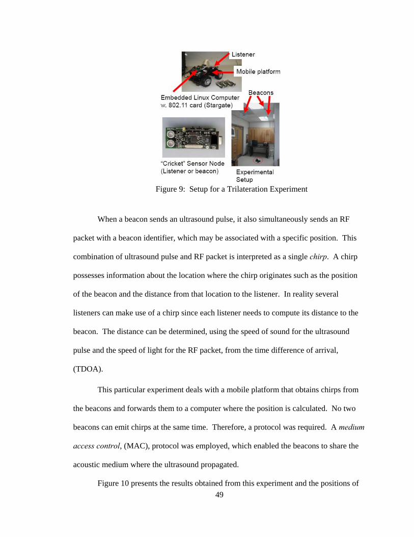
49
Figure 9: Setup for a Trilateration Experiment
When a beacon sends an ultrasound pulse, it also simultaneously sends an RF
packet with a beacon identifier, which may be associated with a specific position. This
combination of ultrasound pulse and RF packet is interpreted as a single chirp. A chirp
possesses information about the location where the chirp originates such as the position
of the beacon and the distance from that location to the listener. In reality several
listeners can make use of a chirp since each listener needs to compute its distance to the
beacon. The distance can be determined, using the speed of sound for the ultrasound
pulse and the speed of light for the RF packet, from the time difference of arrival,
(TDOA).
This particular experiment deals with a mobile platform that obtains chirps from
the beacons and forwards them to a computer where the position is calculated. No two
beacons can emit chirps at the same time. Therefore, a protocol was required. A medium
access control, (MAC), protocol was employed, which enabled the beacons to share the
acoustic medium where the ultrasound propagated.
Figure 10 presents the results obtained from this experiment and the positions of

50
the beacons. The x-marks indicate the trilateration estimates. The smooth curve, which
can be used as ground-truth, shows the trajectory of the mobile platform obtained through
a-posteriori smoothing of the data.
Figure 10: Results of a Trilateration Experiment
Although the experiment was simple, the degree of error, which was an average
of approximately 0.2m in the position estimates, highlights several drawbacks of the
trilateration approach. Most of the drawbacks can be attributed to the fact that the
Cricket localization system was designed for static localization. However, in this case, it
was applied to dynamic tracking of a mobile platform. Salient points, from an analysis of
the experiment, were:
• In order to perform trilateration, three simultaneous measurements are
required. In this case, because of the MAC protocol, the chirps arrive at
different instants of time. If absolutely no filtering is applied, the best
possible result can be obtained using the three most recent chirps. This

51
means that if the listener is moving, only one range measurement is valid
and the other two are outdated. The error is exacerbated considering that
range measurements also have some degree of noise. The solution to this
problem requires projecting the past measurements through a motion
model of the mobile platform in order to apply trilateration to one current
measurement and two past measurements. Hence, filtering is required.
• Sensitivity and error analysis indicate that results are highly dependent on
the configuration of the beacons and on the position of the listener, [46].
For instance, beacons that are almost collinear do not yield good results.
Similarly, when the listener is close to the barycenter of the triangle
formed by the beacons, the sensitivity and errors behave better than when
the listener is in faraway locations.
• The problem of lack of consistency in the error and sensitivity could be
alleviated by placing higher numbers of beacons. However, the listener
would have to choose the best configurations of three beacons to optimize
the error performance of the position estimates.
• At least three measurements from three different beacons are required in
order to obtain a valid position estimate. However, intuitively, one or two
beacons could be used to obtain a raw estimate of position.

52
3.4.1.2. Inertial Measurement Experiment
An Inertial Measurement Unit, (IMU), should improve the location estimation
results obtained in the previous experiment since it contains information about the motion
of the mobile platform. A simple experiment demonstrates the challenges involved in the
use of inertial sensing devices. The experiment consists of simply collecting data from a
static IMU. Six variables were measured with the help of accelerometers and gyroscopes
contained in the IMU. The accelerometers provided three orthogonal accelerations. The
gyroscopes provided three orthogonal angular rates. The IMU used in this experiment is
pictured in Figure 11, which also depicts the measurement axes for the available signals.
Figure 11: The Microstrain’s 3DM-GX1
Inertial Measurement Unit
Figure 12 presents the measured acceleration data and Figure 13 presents the
measured angular rate data. From these results it can be inferred that the position or
attitude of the IMU cannot be determined from the measurements in a straightforward
manner. Acquired measurements present bias and a considerable noise component. The
noise component is especially large in the case of the accelerometers. The
accelerometers also sense the Earth’s gravitation, which makes it difficult to distinguish
the true acceleration from noise and gravity.
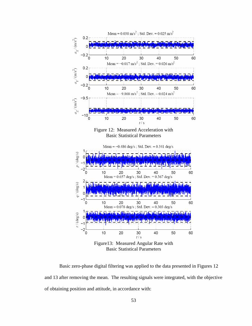
53
Figure 12: Measured Acceleration with
Basic Statistical Parameters
Figure13: Measured Angular Rate with
Basic Statistical Parameters
Basic zero-phase digital filtering was applied to the data presented in Figures 12
and 13 after removing the mean. The resulting signals were integrated, with the objective
of obtaining position and attitude, in accordance with:
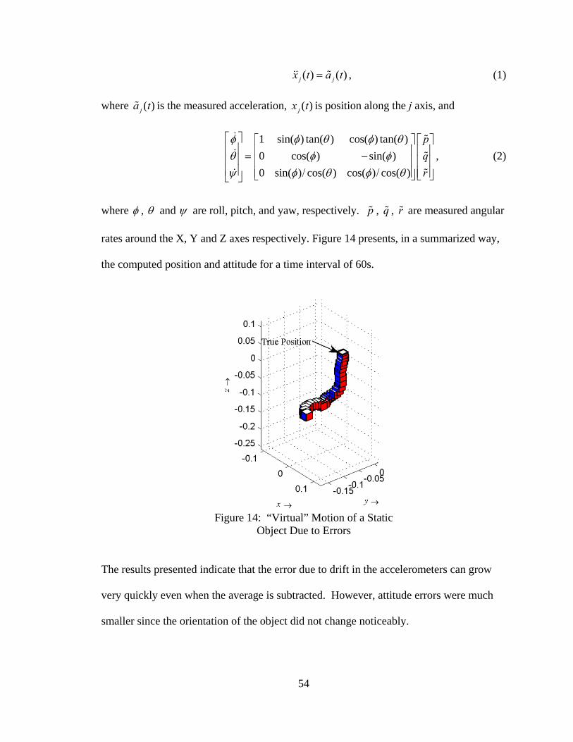
54
( ) ( )j jx t a t= , (1)
where ( )ja t is the measured acceleration, ( )jx t is position along the j axis, and
1 sin( ) tan( ) cos( ) tan( )0 cos( ) sin( )0 sin( ) cos( ) cos( ) cos( )
pqr
φ φ θ φ θθ φ φψ φ θ φ θ
⎡ ⎤ ⎡ ⎤ ⎡ ⎤⎢ ⎥ ⎢ ⎥ ⎢ ⎥= −⎢ ⎥ ⎢ ⎥ ⎢ ⎥⎢ ⎥ / /⎢ ⎥ ⎢ ⎥⎣ ⎦ ⎣ ⎦⎣ ⎦
, (2)
where φ , θ and ψ are roll, pitch, and yaw, respectively. p , q , r are measured angular
rates around the X, Y and Z axes respectively. Figure 14 presents, in a summarized way,
the computed position and attitude for a time interval of 60s.
Figure 14: “Virtual” Motion of a Static
Object Due to Errors
The results presented indicate that the error due to drift in the accelerometers can grow
very quickly even when the average is subtracted. However, attitude errors were much
smaller since the orientation of the object did not change noticeably.

55
3.4.1.3. Summary of Challenges and Issues
The following main challenges have been identified:
• The localization problem based on range measurements is a difficult
problem, [62]. It has been proven that, in the presence of noise, the
localization problem is NP-Hard.
• As seen from the trilateration experiment, measurements may arrive
asynchronously. For instance, in trilateration, at least three simultaneous
range readings are required.
• When using trilateration, choosing different groups of three reference
nodes yields different sensitivity and accuracy.
• Ranging technologies have limited coverage.
• Inertial sensors have significant errors that are non-stationary. If
calculations do not account for these errors the estimation results may
diverge quickly.
• Kinematics of a rigid body is highly nonlinear, as equation 2 indicates.
• Variables of interest in rigid body kinematics are tightly coupled.
• The most practical and inexpensive way to do inertial navigation is with
strap-down inertial measurements systems. However, it may be much
easier to employ gimbaled inertial measurement units, which are more
accurate and sensitive, but bulkier and more expensive.

56
3.4.2. Cooperative Localization and Distributed Estimation
In networked systems, centralized solutions may not be optimal due to several
constraints, which are associated with scalability, robustness and flexibility. This fact is
well known, for instance in ad-hoc networks, which require routing algorithms to build
routes for shuttling information between nodes. Therefore, it is highly desirable to
elaborate a distributed localization solution where the computational and communications
load is distributed evenly among the members of the network.
Making localization a cooperative distributed task improves its coverage,
scalability, flexibility and robustness. The central idea in this research is the possibility
of posing localization as a distributed estimation problem. Figure 15 presents the
cooperative localization process, which takes in a network of four nodes. As indicated in
Figure 15, the problem can be partitioned into three major aspects.
Figure 15: Three Aspects of Cooperative Localization
Each aspect is depicted in different color and represents:
• Local Aspect: The lower blocks represent processing taking place in each
node for the estimation of the node’s position,

57
• Cooperative Aspect: The upper blocks depict the processing component,
which is executed on behalf of other nodes in order to enable cooperative
distributed estimation,
• Information Exchange Aspect: The exchange arrows represent the
information that each node sends to their neighbors as part of the
cooperative estimation process.
The main question consists in finding the appropriate boundaries of problem partitions.
Three questions arise:
• How much processing is going to be performed at the local level?
• What portion of the processing is going to be solved in a distributed
manner?
• What type of information is going to be exchanged?
The more weight that is placed on pure distributed estimation, the greater will be the
amount of information to be exchanged. However, pure local processing will disable the
potential of having more accuracy due to the possibility of exchanging information since
the systems may have to exchange information under any circumstance. Ideally, the
estimation process should allow for a refinement of estimates in a loop such as the one
depicted in Figure 16.

58
Figure16: Cooperative Estimation
3.5. Functional Analysis and Allocation
Following the SE approach, a more detailed functional analysis of the localization
solution yields the main functional modules, which are depicted in Figure 17. The
overall general solution has three main components.
Figure 17: Main Functions of the Cooperative Estimation Solution
Each of the main components is comprised of several sub-units:
• Sensing: This unit is in charge of obtaining physical measurements, which
will enable the system to determine its location. There are two main
categories of sensing devices, which were introduced in section 2.1.4:

59
Proprioceptive: These are devices that can be used by the system
to register its own motion. Sensors of this category are the ones
that provide for performing dead-reckoning, which is also known
as odometry. It can be assumed that proprioceptive measurements
are available at higher sampling rates than measurements from the
complementary exteroceptive category. The proprioceptive
module is only necessary when nodes possess mobility.
Exteroceptive: Odometry cannot be used for long-term position
tracking, due to modeling errors and measurement noise.
However, exteroceptive sensors provide for keeping errors, which
stem from odometry, within bounds. In navigation terms, sensors
of this category are also known as navigation aids.
• Processing: To allow for combining data incoming from the sensing
module and information gathered through the communication interfaces, a
processing device is required. The processing device is required to
execute procedures, which, most likely, would consist of sensor fusion
filters. Accurate positioning of mobile nodes with minimum latency
demands much higher computational power than static node localization.
An additional machine learning module is suggested for localization of
mobile nodes. The learning module would perform online identification
of certain parameters such as drift rates of the inertial sensors, particular
motion patterns of the host vehicle or node carrier, the non-orthogonality
of inertial measurements and lever-arm compensation

60
• Interface: Localization of a wireless node serves an application-specific
purpose. Therefore, there must be a user for the location information.
This module consists of the elements that enable the wireless localization
solution to pass this information to a user or to other nodes. In the latter
case, a node may contribute to the cooperative localization process by
providing its own position estimate to other nodes. Thus, it should be
stressed at this point, that the most viable way to implement cooperative
localization is by making each node share its own position estimate.
Additional to the position estimate, it is important for other nodes to have
a measure of confidence of their position estimate since they may use it in
their own position estimation process.
3.5.1. The “Localizer” – A Conceptual Solution for Cooperative Localization
The third step in the systems engineering approach is design synthesis. Following
these guidelines a conceptual solution for cooperative localization is presented. This
solution can be considered as the vision for this research, which opens the possibility for
generating concrete measurable contributions to the state of the art.
A localizer is an abstraction of the conceptual solution for localization presented
in this work. The “localizer” may exploit hardware already available in its carrier, such
as power, communications interfaces, antennae or even the processing unit. In one
extreme case, the localizer may have the appearance of a small rugged device comprising
all the hardware and software, as presented, in simplified form, in Figure 18.
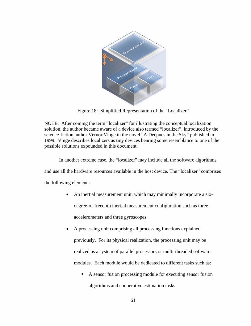
61
Figure 18: Simplified Representation of the “Localizer”
NOTE: After coining the term “localizer” for illustrating the conceptual localization solution, the author became aware of a device also termed “localizer”, introduced by the science-fiction author Vernor Vinge in the novel “A Deepnes in the Sky” published in 1999. Vinge describes localizers as tiny devices bearing some resemblance to one of the possible solutions expounded in this document.
In another extreme case, the “localizer” may include all the software algorithms
and use all the hardware resources available in the host device. The “localizer” comprises
the following elements:
• An inertial measurement unit, which may minimally incorporate a six-
degree-of-freedom inertial measurement configuration such as three
accelerometers and three gyroscopes.
• A processing unit comprising all processing functions explained
previously. For its physical realization, the processing unit may be
realized as a system of parallel processors or multi-threaded software
modules. Each module would be dedicated to different tasks such as:
A sensor fusion processing module for executing sensor fusion
algorithms and cooperative estimation tasks.

62
A communications module for performing all communications
tasks and protocols. This module may also use a signal processor
for assistance in managing software defined radio functions and
range determination. Possibly, only one communications interface
may be necessary for communication with other localizers and
with host devices querying position information.
A management processing module, which may be in charge of
machine learning routines and coordination among the different
processors.
• An antenna or set of antennas in case the communications system is
realized as a MIMO system or in case other geometric relationships are
used for location determination, such as the angle of arrival, (AOA), of a
“chirp.”
The localizer might represent a viable solution for the two motivating examples
expounded in Chapter 1. Additional application scenarios are described below with the
purpose of understanding the function of each module of the localizer.
3.5.2. Application Examples
3.5.2.1. A Localizer-Enabled Cell Phone
One possible application scenario of the localizer may involve incorporating it in
cellular phones for accurate pedestrian navigation. Due to seamless interoperability, cell
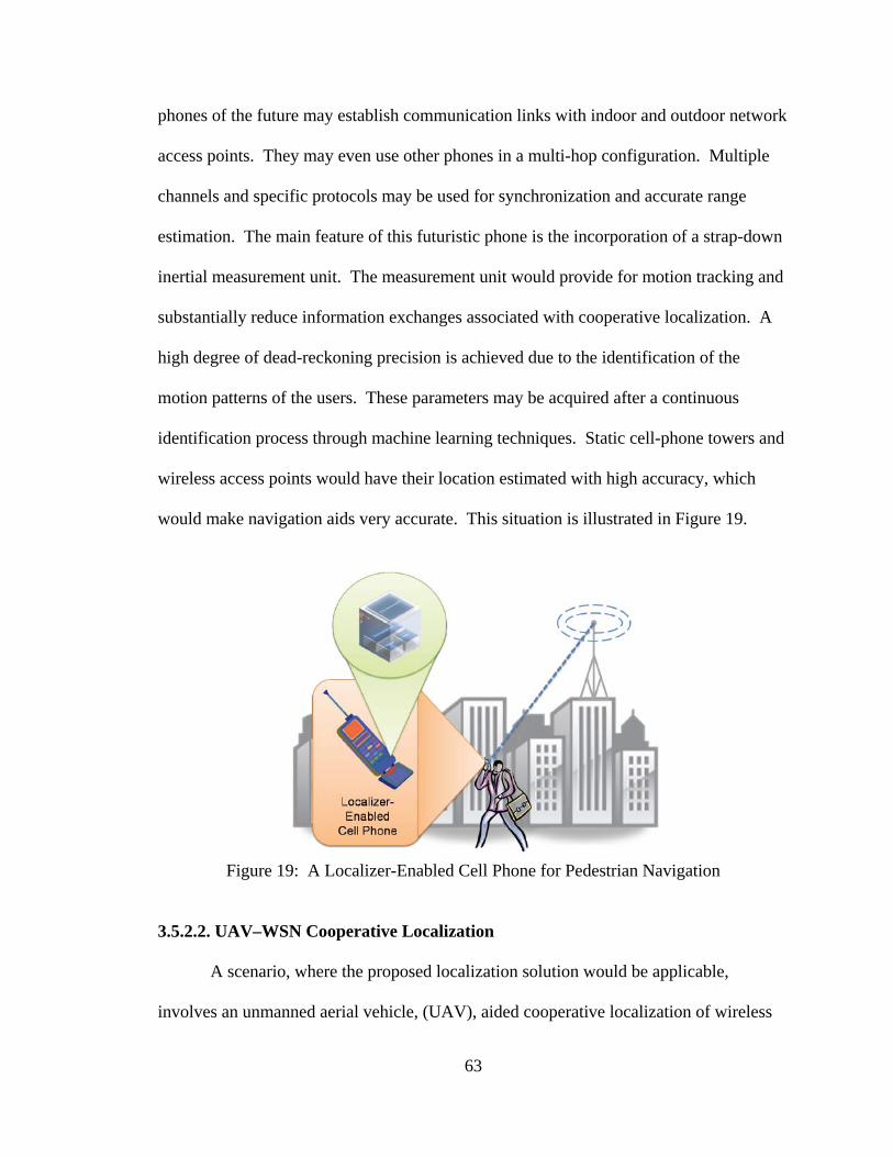
63
phones of the future may establish communication links with indoor and outdoor network
access points. They may even use other phones in a multi-hop configuration. Multiple
channels and specific protocols may be used for synchronization and accurate range
estimation. The main feature of this futuristic phone is the incorporation of a strap-down
inertial measurement unit. The measurement unit would provide for motion tracking and
substantially reduce information exchanges associated with cooperative localization. A
high degree of dead-reckoning precision is achieved due to the identification of the
motion patterns of the users. These parameters may be acquired after a continuous
identification process through machine learning techniques. Static cell-phone towers and
wireless access points would have their location estimated with high accuracy, which
would make navigation aids very accurate. This situation is illustrated in Figure 19.
Figure 19: A Localizer-Enabled Cell Phone for Pedestrian Navigation
3.5.2.2. UAV–WSN Cooperative Localization
A scenario, where the proposed localization solution would be applicable,
involves an unmanned aerial vehicle, (UAV), aided cooperative localization of wireless

64
sensor networks. For instance, an environmental monitoring WSN may be deployed
randomly by UAVs in a location with severe LOS obstruction with respect to GPS-
satellites. WSN nodes may be equipped with a localizer, which would allow them to
cooperatively find their relative location. However, if data needs to be collected using
absolute location information, there should be a mechanism that would allow the nodes to
determine their absolute location. A localizer-enabled UAV could be used for
“spreading” location information among the WSN nodes just after deployment. This
situation is illustrated in Figure 20.
Figure 20: UAV-WSN Cooperative Localization
The motion of the UAV would allow it to broadcast chirps from different
locations. The chirps would allow the WSN nodes to estimate their own position
information. Not all nodes would need to find their location. Certain nodes could use
similar cooperative localization mechanisms for refining the position estimates
independently of the UAV. The cooperative localization mechanisms would provide for
achieving complete coverage of the network.
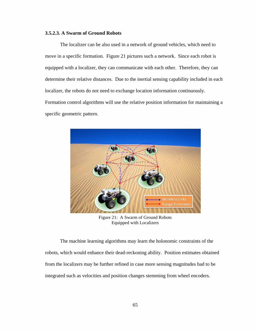
65
3.5.2.3. A Swarm of Ground Robots
The localizer can be also used in a network of ground vehicles, which need to
move in a specific formation. Figure 21 pictures such a network. Since each robot is
equipped with a localizer, they can communicate with each other. Therefore, they can
determine their relative distances. Due to the inertial sensing capability included in each
localizer, the robots do not need to exchange location information continuously.
Formation control algorithms will use the relative position information for maintaining a
specific geometric pattern.
Figure 21: A Swarm of Ground Robots
Equipped with Localizers
The machine learning algorithms may learn the holonomic constraints of the
robots, which would enhance their dead-reckoning ability. Position estimates obtained
from the localizers may be further refined in case more sensing magnitudes had to be
integrated such as velocities and position changes stemming from wheel encoders.
66
3.6. The Role of Ranging
Navigation aids used in this research used range measurements such as inter-node
distances. In the remainder of this document, it is assumed that range measurements are
available, even under adverse conditions, which is the primary situation in indoor
environments. Indoor environments pose the main challenge to current ranging methods
due to the difficulty of range estimation under Undetected Direct Path, (UDP),
conditions, [63]. These conditions arise in cluttered environments with severe multi-path
propagation characteristics. Under these conditions nodes do not have Line of Sight,
(LOS), connectivity. The cooperative nature of the localization scheme proposed in this
research makes the estimation of very long ranges unnecessary. However, most
researchers agree that, due to intense research work in Ultra-Wideband, (UWB),
modulation techniques, in the near future range measurements may be available as a
byproduct of the networking functionality of wireless networking interfaces, [64]. The
main advantages and challenges of UWB localization, as well as an outline of techniques
and error bounds, are covered in a tutorial manner in, [65].
3.7. Summary
The localization problem was analyzed and considered most relevant aspects from
the systems engineering perspective. Initially, requirements and metrics were defined.
Two preliminary experiments served for identifying key issues in localization, which
showed it to be a non-trivial problem. Function allocation exposed the structure and
modules necessary for creating a conceptual solution, which may be applied to a variety
of scenarios. Finally, the “localizer” was presented with some examples illustrating its

67
use and capabilities. A localizer may be realized as a stand-alone device. Alternatively,
its functions may be embedded in the computers of the host vehicle or carrier. The main
characteristic of the localizer consists of the integration of three aspects:
• A wireless network interface with the functions of communications and
range measurements,
• An inertial measurement unit,
• One or more processing devices executing routines for the implementation
of protocols, for recursive state estimation and for continuous on-line
calibration.
68
Chapter 4
Cooperative Localization in the Case of Fixed Nodes
Several aspects of the conceptual solution were presented in the previous chapter.
The best way to approach solving a complex problem, which includes many functional
components and fields, is to isolate the different aspects of the problem by applying a
“divide and conquer” approach. In the divide phase, the nodes were considered to be
fixed. The fixed node assumption allowed key aspects of the problem to be isolated.
However, the fixed node idea is not an assumption but the relevant condition in certain
problems. The problem of localization in Wireless Sensor Networks, (WSNs), which
was outlined in the introduction, is a fixed node localization problem.
This chapter develops two main ideas that were key in this research:
• Probabilistic estimation: It is shown that probabilistic approaches can
override limitations inherent to deterministic solutions such as those using
graph rigidity, trilateration or other similar ideas.
• Cooperative localization: It is proven that devices can exchange
information and use it for determining their own location in a cooperative
and distributed manner.
The associated aspects of mobility and the protocols underlying cooperative localization
are handled in subsequent chapters. For practical implementation of the localization
algorithms, which are presented in this chapter, additional aspects are explored.

69
Computational and energy constraints inherent to WSN nodes, which were used while
seeking to minimize the complexity of the estimation algorithms, are presented.
Additionally, the number of messages, required to be exchanged, between nodes to
achieve accurate localization was investigated.
4.1. Probabilistic Approach to Localization
In section 3.4.1.1, it was shown that trilateration may not be the best solution for
determining the position of a node. Obtaining the position from pure geometry in a
closed form expression or through an iterative solution is regarded as the deterministic
approach to localization. Probabilistic techniques constitute an alternative approach.
One of the main advantages of probabilistic techniques is that they facilitate the
consideration of uncertainty, which is always present in real-world applications. The
main sources of uncertainty reside in the inaccuracy of dynamic models and in the
measurement of noise.
This section introduces the probabilistic estimation framework as applied to
localization. The approach follows the one presented in, [16]. In general, and not only
for fixed nodes, the localization problem can be viewed as a continuous Markov process.
The state of the system, ( tx ), evolves with time and is driven by the controls, ( tu ). The
system is Markovian because the current state depends only on the previous state, ( 1tx − ),
and the control action. In other words, to predict the next state, it is only necessary to
know the current state, the control that is being applied and the conditional probability
functions. The state is not directly observable. Only measurements, ( tz ), are available.
The measurements are probabilistic projections of the state. Measurements contain noise.

70
Since the state is “hidden behind” the measurements, the model of the evolution of the
position in time can be regarded as a Hidden Markov Model, (HMM), or as a Dynamic
Bayes Network, (DBN). It is important to note that the state is not the position. The state
is a collection of variables that completely describe the system. Hence, the state may also
incorporate the current velocity and rotational speed in the case of moving nodes. A
diagrammatic depiction of a HMM is presented in Figure 22.
Figure 22: Localization as a Hidden Markov Model:
From [16]
A paramount change in perception occurs when applying probabilistic methods to
the problem of localization. The position of an object or node cannot be viewed as
possessing a fixed value, which can be directly measured. Instead, position is viewed as
stochastic in nature and, the value associated with position, is termed belief. A belief can
be understood as the node’s internal knowledge about the state. The belief also
incorporates the uncertainty inherent to the non-absolute knowledge about the state. In
statistical terms, a belief is simply a probability density function. The belief distribution
represents the probability of any hypothetical state value.
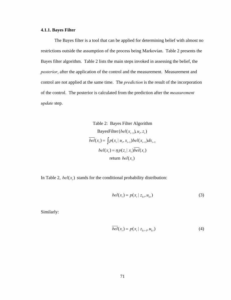
71
4.1.1. Bayes Filter
The Bayes filter is a tool that can be applied for determining belief with almost no
restrictions outside the assumption of the process being Markovian. Table 2 presents the
Bayes filter algorithm. Table 2 lists the main steps invoked in assessing the belief, the
posterior, after the application of the control and the measurement. Measurement and
control are not applied at the same time. The prediction is the result of the incorporation
of the control. The posterior is calculated from the prediction after the measurement
update step.
Table 2: Bayes Filter Algorithm
BayesFilter 1( ( ) )t t tbel x u z− , ,
1 1 1( ) ( ) ( )t t t t t tbel x p x u x bel x dx− − −= | ,∫
( ) ( ) ( )t t t tbel x p z x bel xη= |
return ( )tbel x
In Table 2, ( )tbel x stands for the conditional probability distribution:
1 1( ) ( )t t t tbel x p x z u: := | , (3)
Similarly:
1 1 1( ) ( )t t t tbel x p x z u: − := | , (4)

72
For calculating the posterior, three probability distributions are required:
• The initial belief: 0( )p x ,
• The transition probability: 1( )t t tp x u x −| , ,
• The measurement probability: ( )t tp z x| .
4.1.1.1. Illustrating the Experiment
In an experiment similar to the one performed in Section 3.4.1.1, beacon nodes
send chirps to a static listener. Given that the device to be localized is static makes the
prediction calculation step unnecessary. Figure 23 depicts the configuration of the
beacons and the listener.
Figure 23: Configuration of Beacons and a Listener
Figures 24 through 26 show the sequential application of the Bayes filter. The
assumptions are that range measurements are always noisy and that the measurement
noise has Gaussian distribution. Therefore, the location of a listener belief can be
represented by an annular distribution centered on the beacon. The belief after one range
measurement is presented in Figure 24.
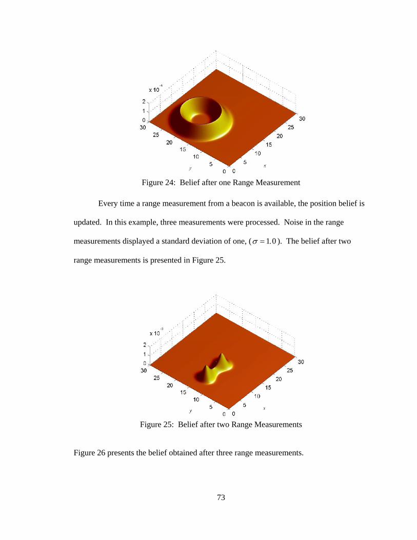
73
Figure 24: Belief after one Range Measurement
Every time a range measurement from a beacon is available, the position belief is
updated. In this example, three measurements were processed. Noise in the range
measurements displayed a standard deviation of one, ( 1 0σ = . ). The belief after two
range measurements is presented in Figure 25.
Figure 25: Belief after two Range Measurements
Figure 26 presents the belief obtained after three range measurements.
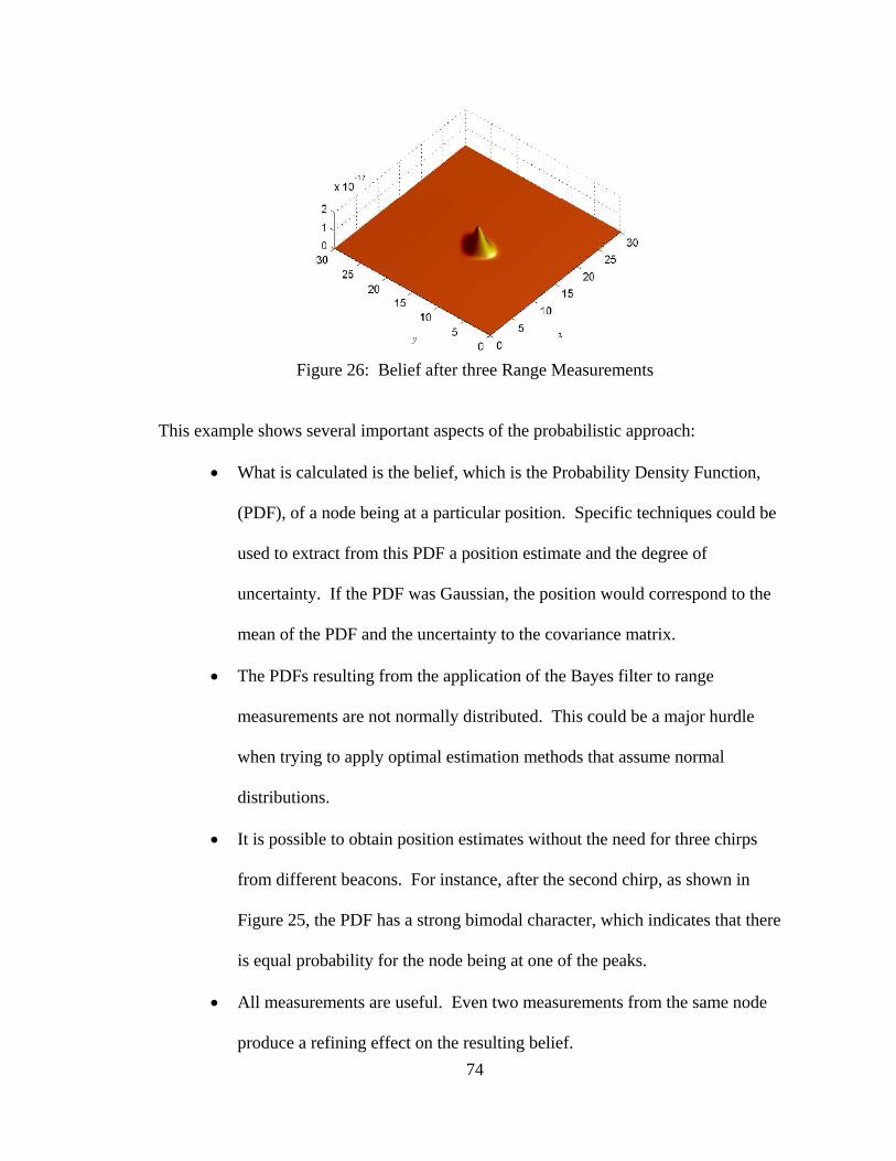
74
Figure 26: Belief after three Range Measurements
This example shows several important aspects of the probabilistic approach:
• What is calculated is the belief, which is the Probability Density Function,
(PDF), of a node being at a particular position. Specific techniques could be
used to extract from this PDF a position estimate and the degree of
uncertainty. If the PDF was Gaussian, the position would correspond to the
mean of the PDF and the uncertainty to the covariance matrix.
• The PDFs resulting from the application of the Bayes filter to range
measurements are not normally distributed. This could be a major hurdle
when trying to apply optimal estimation methods that assume normal
distributions.
• It is possible to obtain position estimates without the need for three chirps
from different beacons. For instance, after the second chirp, as shown in
Figure 25, the PDF has a strong bimodal character, which indicates that there
is equal probability for the node being at one of the peaks.
• All measurements are useful. Even two measurements from the same node
produce a refining effect on the resulting belief.

75
4.1.2. Particle Filters
Graphs in previous sections were computed using the generic Bayes filter, which
was evaluated numerically on a grid with almost 300 cells per side. However,
localization needs to be implemented in embedded devices. Therefore, working with
such a degree of resolution or even symbolically may not be feasible as a result of
memory and computational constraints. There are two main possibilities for the practical
representation of beliefs; Gaussian and non-parametric. Due to the non-Gaussian nature
of the beliefs resulting from applying measurement updates stemming from range
measurements, this section considers only non-parametric belief representations. Non-
parametric belief representations work with sampled versions of the distributions. The
two popular varieties of sampled representations are histogram filters and particle filters.
The particle filter representation is known to possess a high level of robustness and there
are a number of techniques that make it computationally tractable. The generic particle
filter algorithm, which can be viewed as a Monte Carlo approximation of the Bayes filter,
is listed in Table 3.
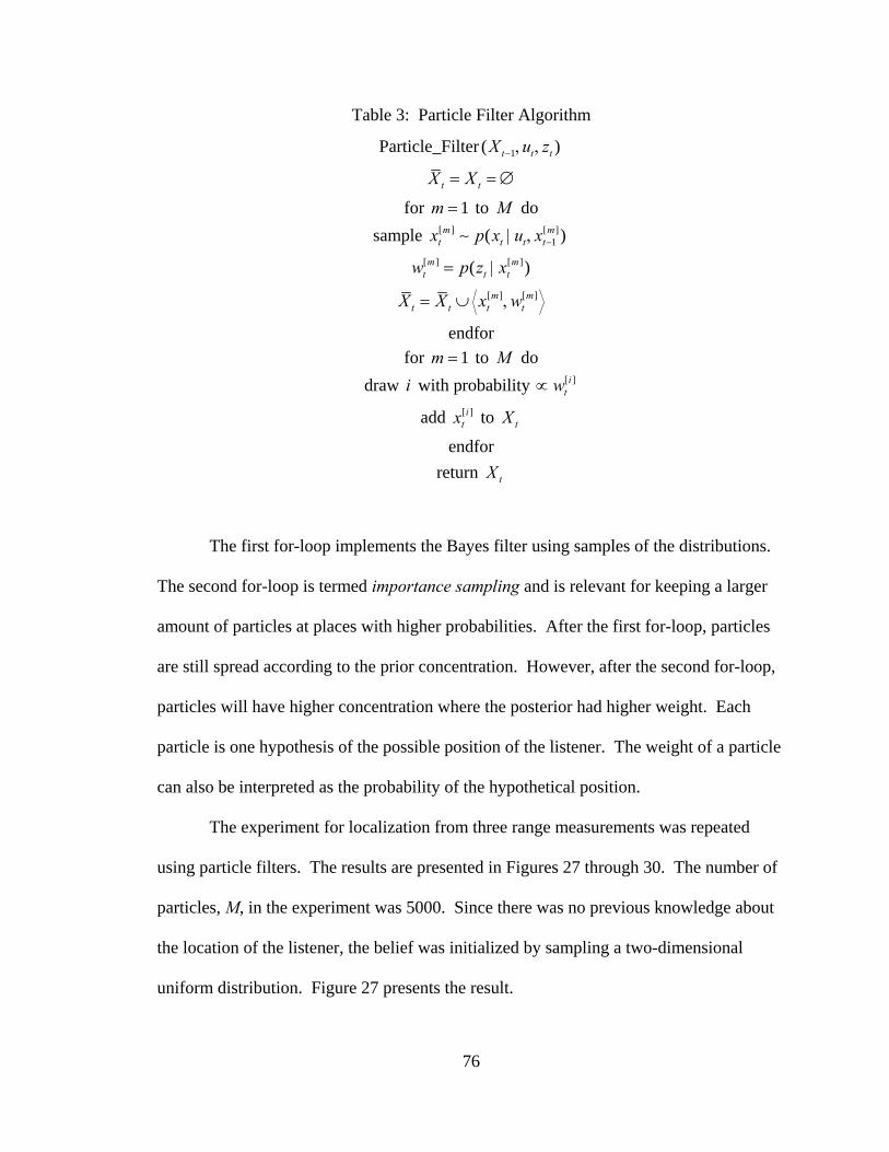
76
Table 3: Particle Filter Algorithm
Particle_Filter 1( )t t tX u z− , ,
t tX X= = ∅
for 1m = to M do sample [ ] [ ]
1( )m mt t t tx p x u x −| ,∼
[ ] [ ]( )m mt t tw p z x= |
[ ] [ ]m mt t t tX X x w= ∪ ,
endfor for 1m = to M do
draw i with probability [ ]itw∝
add [ ]itx to tX
endfor return tX
The first for-loop implements the Bayes filter using samples of the distributions.
The second for-loop is termed importance sampling and is relevant for keeping a larger
amount of particles at places with higher probabilities. After the first for-loop, particles
are still spread according to the prior concentration. However, after the second for-loop,
particles will have higher concentration where the posterior had higher weight. Each
particle is one hypothesis of the possible position of the listener. The weight of a particle
can also be interpreted as the probability of the hypothetical position.
The experiment for localization from three range measurements was repeated
using particle filters. The results are presented in Figures 27 through 30. The number of
particles, M, in the experiment was 5000. Since there was no previous knowledge about
the location of the listener, the belief was initialized by sampling a two-dimensional
uniform distribution. Figure 27 presents the result.

77
Figure 27: Particle Filter Initialization
Figure 28 shows the belief after the first range measurement and after resampling, which
is also known as importance sampling.
Figure 28: Particles after the First
Range Measurement
Figure 29 presents the belief after the second range measurement.
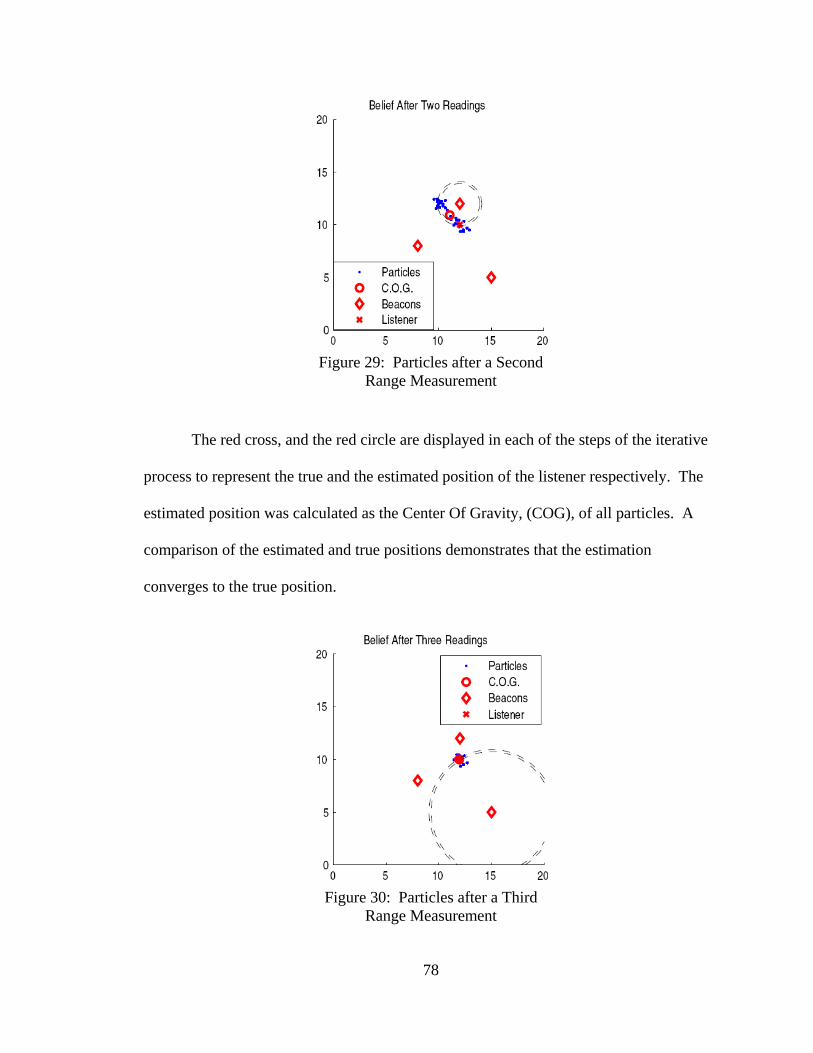
78
Figure 29: Particles after a Second
Range Measurement
The red cross, and the red circle are displayed in each of the steps of the iterative
process to represent the true and the estimated position of the listener respectively. The
estimated position was calculated as the Center Of Gravity, (COG), of all particles. A
comparison of the estimated and true positions demonstrates that the estimation
converges to the true position.
Figure 30: Particles after a Third
Range Measurement
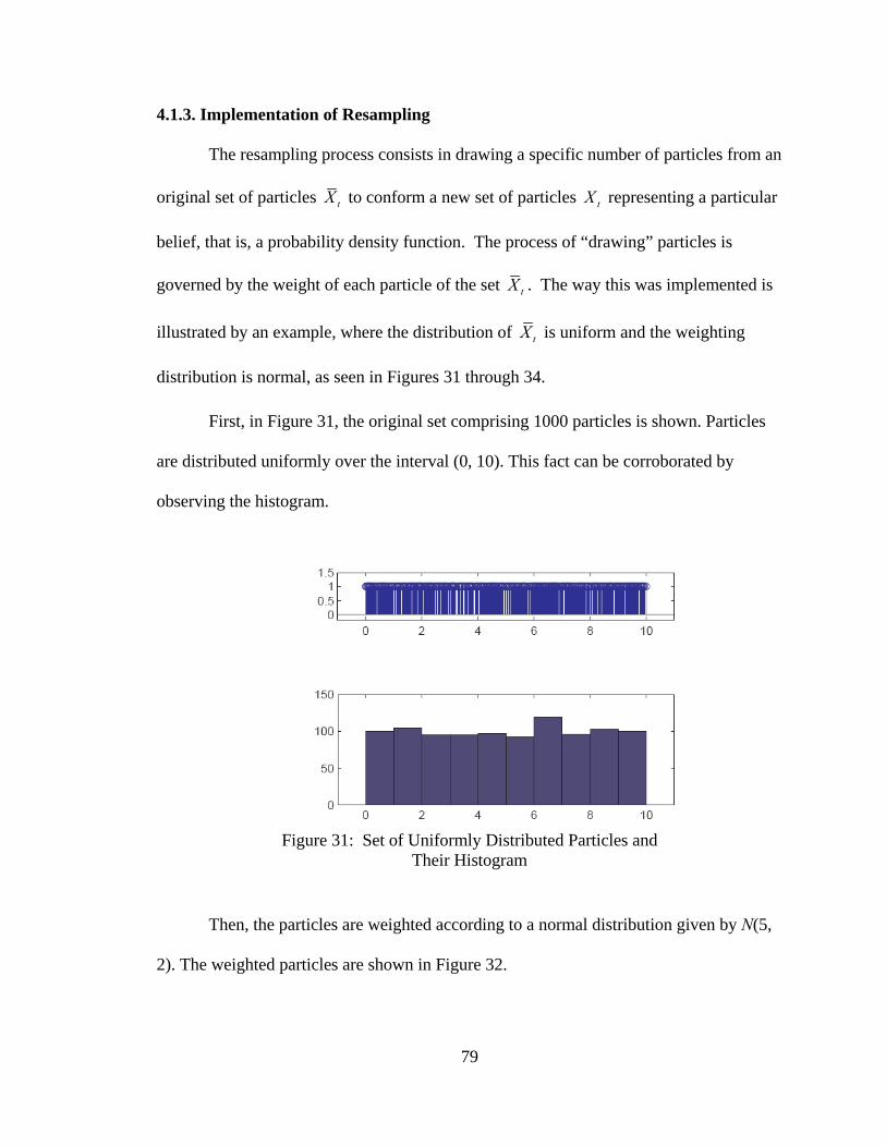
79
4.1.3. Implementation of Resampling
The resampling process consists in drawing a specific number of particles from an
original set of particles tX to conform a new set of particles tX representing a particular
belief, that is, a probability density function. The process of “drawing” particles is
governed by the weight of each particle of the set tX . The way this was implemented is
illustrated by an example, where the distribution of tX is uniform and the weighting
distribution is normal, as seen in Figures 31 through 34.
First, in Figure 31, the original set comprising 1000 particles is shown. Particles
are distributed uniformly over the interval (0, 10). This fact can be corroborated by
observing the histogram.
Figure 31: Set of Uniformly Distributed Particles and
Their Histogram
Then, the particles are weighted according to a normal distribution given by N(5,
2). The weighted particles are shown in Figure 32.

80
Figure 32: Weighted Particles
Figure 33 shows the cumulative sum of the weights. After that, N random values
are generated according to a uniform distribution U(0, 1). These values are used to
perform an interpolation finding the indexes of the corresponding particles. This can be
thought as finding the x value for each y generated value. The concrete MATLAB
command used is:
newix = interp1(cumul,1:N,ix,’nearest’,’extrap’)
Figure 33: Cumulative Weight of Weighted Particles
Then, the new particle set consists of the particles with the indexes obtained from
the function mentioned above. The new set is depicted in Figure 34. The corresponding
histogram shows that the particles are distributed according to the weighting distribution
N(5, 2).
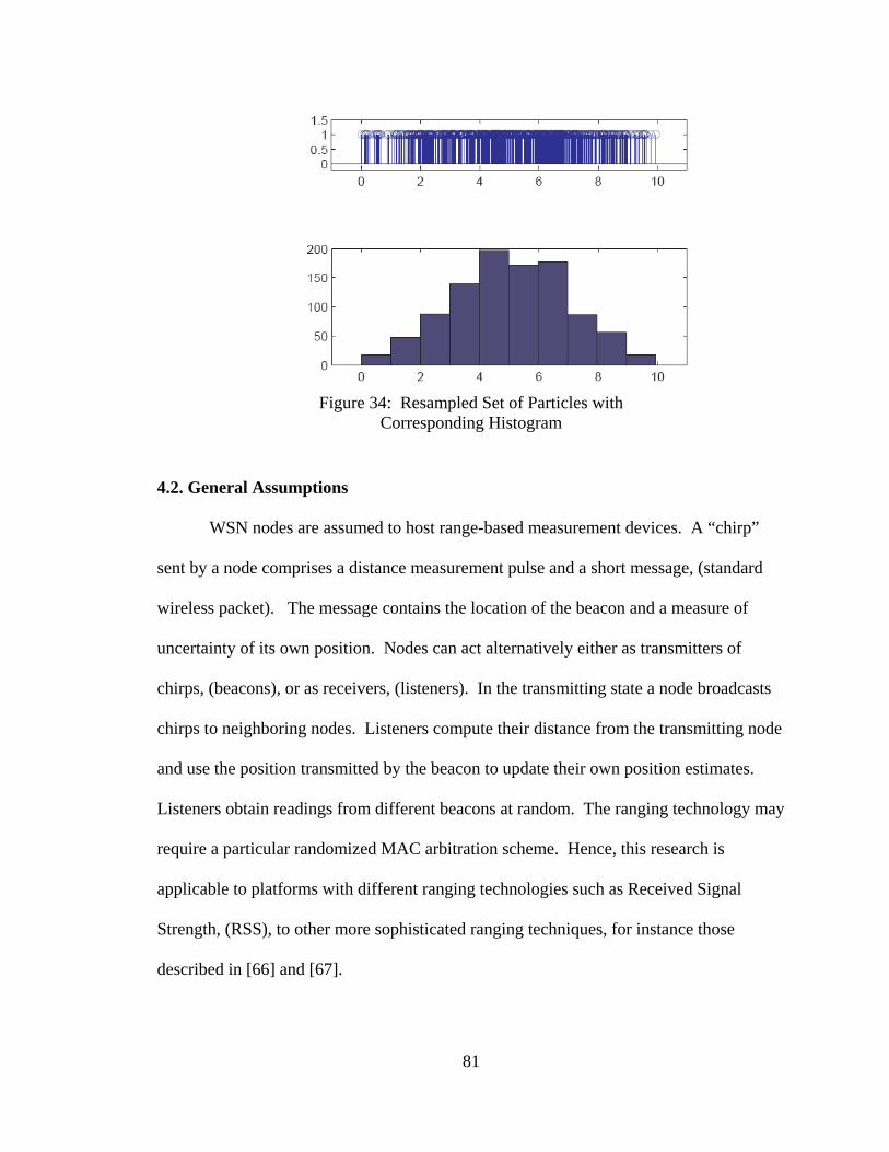
81
Figure 34: Resampled Set of Particles with
Corresponding Histogram
4.2. General Assumptions
WSN nodes are assumed to host range-based measurement devices. A “chirp”
sent by a node comprises a distance measurement pulse and a short message, (standard
wireless packet). The message contains the location of the beacon and a measure of
uncertainty of its own position. Nodes can act alternatively either as transmitters of
chirps, (beacons), or as receivers, (listeners). In the transmitting state a node broadcasts
chirps to neighboring nodes. Listeners compute their distance from the transmitting node
and use the position transmitted by the beacon to update their own position estimates.
Listeners obtain readings from different beacons at random. The ranging technology may
require a particular randomized MAC arbitration scheme. Hence, this research is
applicable to platforms with different ranging technologies such as Received Signal
Strength, (RSS), to other more sophisticated ranging techniques, for instance those
described in [66] and [67].
82
Two scenarios, incremental localization and concurrent localization, are analyzed
in order to define the localization problem, [68]. In both scenarios, the ranging device
has a specific coverage area. In the incremental localization scenario, reference nodes
broadcast their position to nodes within their coverage area. As soon as a node has a
good position estimate it begins to broadcast its position to other nodes, which expands
the region of coverage for localization. In concurrent localization all nodes start the
localization process simultaneously. In both scenarios, nodes cooperate to obtain the
final position estimates, which leads to the term cooperative localization. Therefore, in
cooperative localization, WSN nodes do not rely on a central platform to assist in the
localization process. Consequently, the algorithms are characterized as distributed. In
both scenarios, it is assumed that there is an underlying MAC layer protocol striving to
minimize the overhead of information packets exchanged for coordination. It is also
assumed that localization packets, (chirps), constitute the core of the information
exchange necessary for enabling localization.
Given that communications was the key factor impacting network lifetime in
WSNs, the main metric considered, to reach final localization estimates, was the total
number of chirps broadcasted, [69]. The main concern was the convergence time of the
algorithm measured by the number of chirps. Slower convergence implies that more
messages must be exchanged. Thus, the message complexity of the distributed algorithm
employed for localization was crucial to assess its impact on the energy consumption and
the lifetime of the WSN.

83
4.3. Varying the Number of Particles
In Section 4.1.2 the localization process using a particle filter, which consisted of
5000 particles was illustrated. The large amount of memory required for localization
motivated an investigation of the effect of changing the amount of particles. Reduction
of the number of particles required would make the method applicable to devices with
constrained computational and memory storage resources. However, convergence time is
severely affected by the number of particles, which will be demonstrated in subsequent
paragraphs.
In the experiments performed, the Crámer-Rao bound was not calculated, [48].
Therefore, convergence was assumed to be reached when the COG of the particles was
within one standard deviation of the measurements. The experiment was run twenty
times with different random seeds. The results presented in Figure 35 are the averages of
twenty runs.
Figure 35: Convergence as a Function of Particle Size

84
On average, approximately seven chirps are required in order to reach final
estimates. These results were corroborated by applying the binomial distribution. The
problem is that fast convergence, (7 chirps in this case), can only be obtained with a
number of particles greater than 1000. Other experiments demonstrated that
approximately 500 particles were necessary if they were initialized with a flat annular
distribution around the beacon, after the first reading, instead of a uniform distribution.
However, even 500 particles impose a significant burden on the reduced memory and
computational resources available in WSN nodes.
Significant memory and computational requirements exist to yield fast
convergence in sequential Monte-Carlo estimation. Reducing the number of particles
slows convergence. Slow convergence is particularly undesirable when faced with the
prospect of trying to apply this method to tracking mobile nodes. Slow convergence
would also increase the amount of chirps required, which would incur high energy
expenditures. An additional problem related to reducing the number of particles is that
particle filters base their robustness on keeping particles, (hypothesis) with low
probability, (weight).
4.4. Adapting Particle Filters
The two elements that are essential to estimation are the belief representation and
the estimation law. When the belief is approximated by a Gaussian distribution, the
optimal estimation law, which minimizes the sum of the squared errors, is given by the
Kalman filter. When the belief is strongly non-Gaussian the belief may be approximated
by a set of particles. The main objective pursued in this research was to reduce the

85
amount of particles used in particle filters while maintaining their positive properties such
as simplicity, robustness and fast convergence. Previous experimentation has shown that
a reduction in the number of particles causes an increment in the amount of chirps
necessary to achieve localization. The main reason for this degradation lies in the fact
that fewer particles cannot represent the actual belief with sufficient accuracy. Therefore,
if fewer particles are used, they should not be generated “randomly” as in the original
formulation of the Monte Carlo approximation. Hence, a smoother trade-off of accuracy
and convergence versus number of particles is sought, (graceful degradation).
This research proposed a nonlinear estimation algorithm. The algorithm is based
on a suboptimal update rule. The rule yields extreme simplicity and flexibility due to its
straightforward geometric interpretation. Since it handles position as a belief, the
algorithm conserves the probabilistic nature of sequential estimation methods.
Furthermore, it incorporates a heuristic certainty measure, which resembles the
covariance measure of belief in a parametric implementation of the Bayes filter.
If a WSN node is static, the hypotheses of a particle filter do not move.
Therefore, particles are only subject to the importance resampling process. In the
resampling process the most likely hypothesis is drawn, with higher probability, to
generate a new set of particles. Due to this research, it is proposed that particles not be
resampled. Instead, particles should be moved to relevant spots as the sequential
estimation process proceeds, (adaptation). The term “particle” is kept and it is still used
for representing a hypothesis of the state that needs to be estimated, which is the position
of the node. It is possible to determine the optimal next estimate by applying optimal
filtering theory. This approach would lead to a parametric implementation of the Bayes
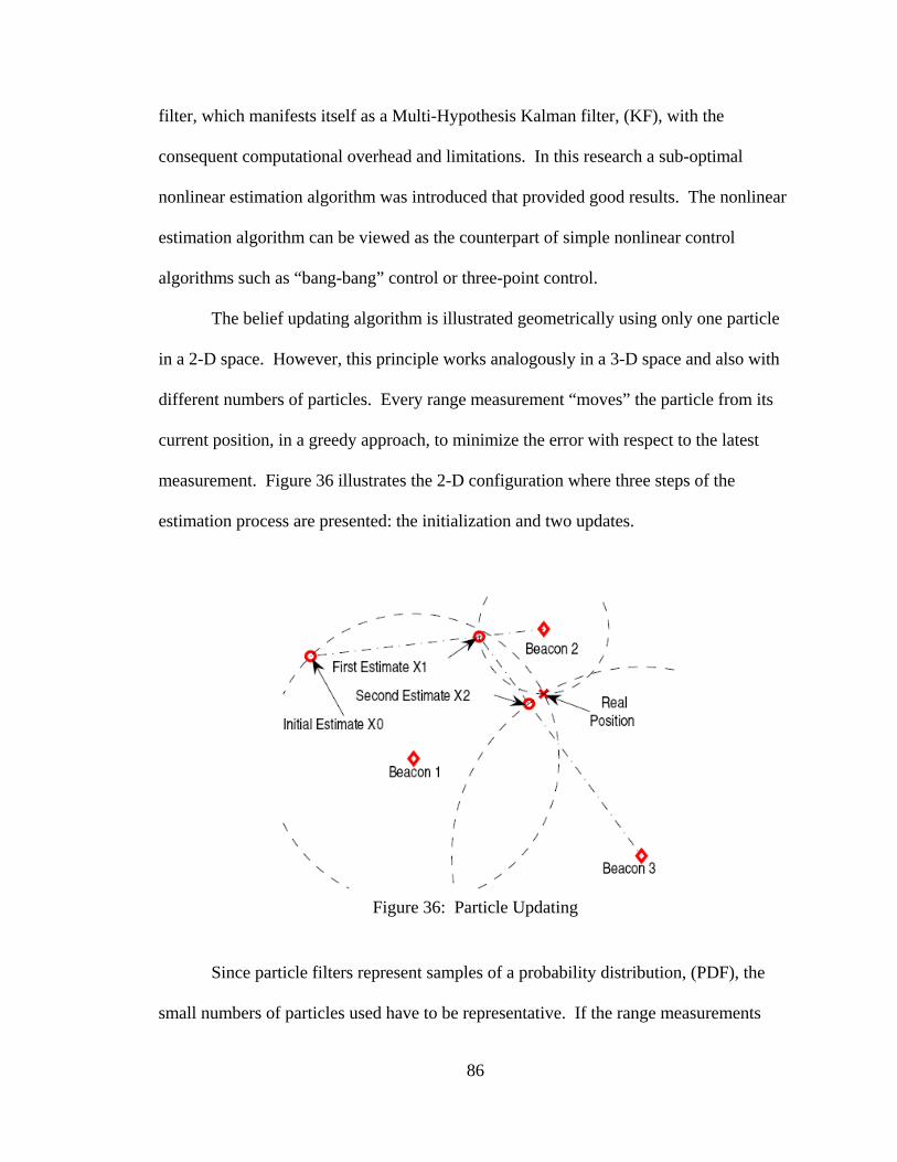
86
filter, which manifests itself as a Multi-Hypothesis Kalman filter, (KF), with the
consequent computational overhead and limitations. In this research a sub-optimal
nonlinear estimation algorithm was introduced that provided good results. The nonlinear
estimation algorithm can be viewed as the counterpart of simple nonlinear control
algorithms such as “bang-bang” control or three-point control.
The belief updating algorithm is illustrated geometrically using only one particle
in a 2-D space. However, this principle works analogously in a 3-D space and also with
different numbers of particles. Every range measurement “moves” the particle from its
current position, in a greedy approach, to minimize the error with respect to the latest
measurement. Figure 36 illustrates the 2-D configuration where three steps of the
estimation process are presented: the initialization and two updates.
Figure 36: Particle Updating
Since particle filters represent samples of a probability distribution, (PDF), the
small numbers of particles used have to be representative. If the range measurements
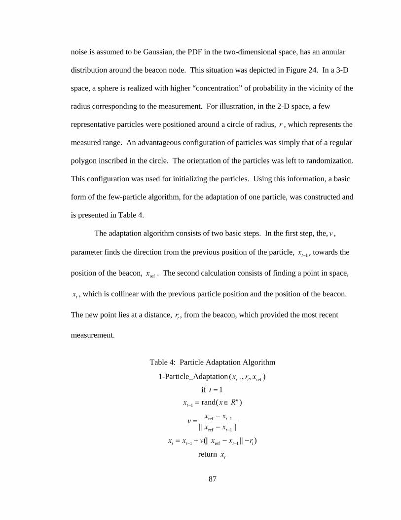
87
noise is assumed to be Gaussian, the PDF in the two-dimensional space, has an annular
distribution around the beacon node. This situation was depicted in Figure 24. In a 3-D
space, a sphere is realized with higher “concentration” of probability in the vicinity of the
radius corresponding to the measurement. For illustration, in the 2-D space, a few
representative particles were positioned around a circle of radius, r , which represents the
measured range. An advantageous configuration of particles was simply that of a regular
polygon inscribed in the circle. The orientation of the particles was left to randomization.
This configuration was used for initializing the particles. Using this information, a basic
form of the few-particle algorithm, for the adaptation of one particle, was constructed and
is presented in Table 4.
The adaptation algorithm consists of two basic steps. In the first step, the, v ,
parameter finds the direction from the previous position of the particle, 1tx − , towards the
position of the beacon, refx . The second calculation consists of finding a point in space,
tx , which is collinear with the previous particle position and the position of the beacon.
The new point lies at a distance, tr , from the beacon, which provided the most recent
measurement.
Table 4: Particle Adaptation Algorithm
1-Particle_Adaptation 1 ref( )t tx r x− , ,
if 1t =
1 rand( )ntx x R− = ∈
ref 1
ref 1
t
t
x xvx x
−
−
−=|| − ||
1 ref 1( )t t t tx x v x x r− −= + || − || −
return tx

88
If more particles are used, the particle adaptation algorithm is performed on each
of the particles. Actual position estimates can be computed via the weighted average,
(center of gravity), of the particles and is given by:
1
ˆpN
i ii
x w x=
= ⋅∑ . (5)
If only the Table 4 update rule is used, nodes holding just one particle, which are
surrounded by beacons, estimate their location rather quickly. In addition, if the node
degree is high the location estimate is derived even more quickly. However, localization
converges rather slowly in the case where beacons are positioned on one side only. This
situation occurs always at the borders of the network. Therefore, several particles are
required to have more hypotheses and to find convergence. The weight, w , of a particle
is proportional to the probability of the distance of the particle to the beacon, ( pd ).
Assuming that range measurements, ( )rN r σ, are distributed normally, with, r , the range
measurement and rσ the standard deviation of the measurement, the weight can be
calculated by:
2
2
( )1Pr( ) exp2p
p rr
d rw d r σ
η σ⎛ ⎞−
= | , = −⎜ ⎟⎝ ⎠
. (6)
The factor 1 η/ is used for normalization of the particles. The particles conform
to a discrete distribution, which approximates a Gaussian, ( )rN r σ, on the distance to the
beacon. In order to avoid numerical issues, a probability threshold, Thrw , can be defined
to eliminate particles with very low probability. This method would work in a similar

89
way even if a different unimodal distribution is assumed, for instance a triangular
distribution, which would yield significant computational simplicity for wireless sensor
nodes.
Parameters r and rσ can be used when the position of the beacon is assumed to
be known with 100% certainty. However, in cooperative localization, imperfectly
localized nodes act as beacons for other nodes, which have more uncertainty in their
location estimates. Therefore, the uncertainty in the position of the beacon has to be
taken into account. Assuming that nodes possess a heuristic “certainty” measure,
[0 1]c∈ , , the standard deviation used to evaluate the weight of the particles can be
updated using:
1 log( )r cσ σ α= − . (7)
The factor α depends on the application and the certainty measure adopted. It
can be verified that if the beacon knows its position with absolute certainty, ( 1c = ), the
standard deviation used in the weight evaluation is simply the same as the one
corresponding to the measurements, rσ . However, if the certainty is low, the weighting
Gaussian is wider. Such a Gaussian has the effect of keeping particles that would be
otherwise eliminated if a more constrained distribution was used.
As mentioned before, the significance of the location certainty, c , becomes
apparent in the situation of incremental localization. Unlocalized nodes start with a
certainty of zero and reference nodes start with certainty close to one since their location
is assumed to be known. It is expected that every update helps to increase the location
certainty of a node. This expectation is reasonable in view of the assumption that there
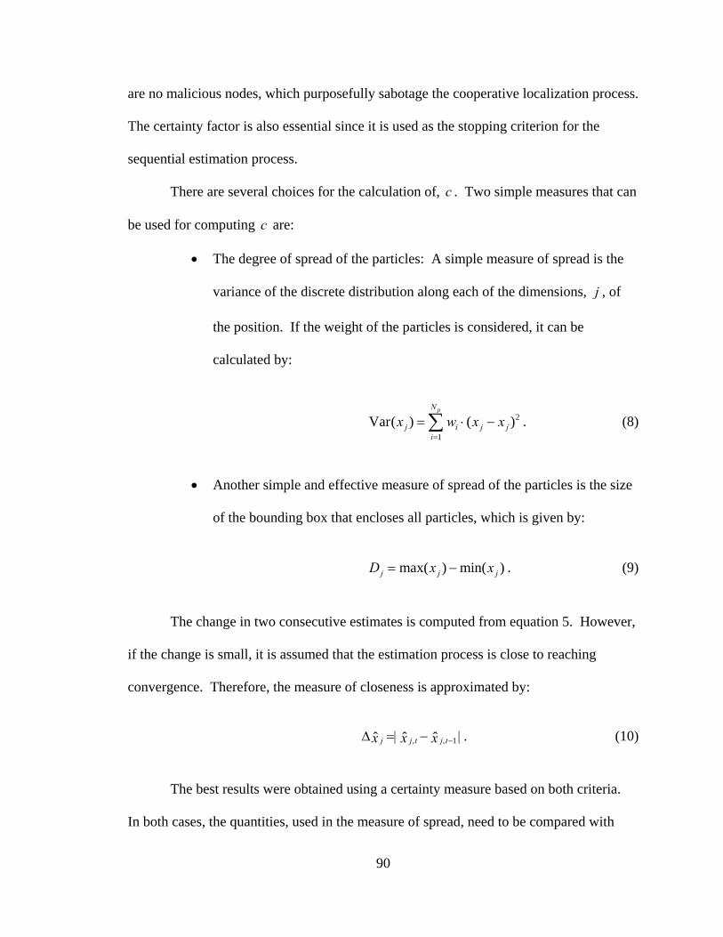
90
are no malicious nodes, which purposefully sabotage the cooperative localization process.
The certainty factor is also essential since it is used as the stopping criterion for the
sequential estimation process.
There are several choices for the calculation of, c . Two simple measures that can
be used for computing c are:
• The degree of spread of the particles: A simple measure of spread is the
variance of the discrete distribution along each of the dimensions, j , of
the position. If the weight of the particles is considered, it can be
calculated by:
2
1
Var( ) ( )pN
j i j ji
x w x x=
= ⋅ −∑ . (8)
• Another simple and effective measure of spread of the particles is the size
of the bounding box that encloses all particles, which is given by:
max( ) min( )j j jD x x= − . (9)
The change in two consecutive estimates is computed from equation 5. However,
if the change is small, it is assumed that the estimation process is close to reaching
convergence. Therefore, the measure of closeness is approximated by:
1ˆ ˆ ˆj j t j tx x x, , −Δ =| − | . (10)
The best results were obtained using a certainty measure based on both criteria.
In both cases, the quantities, used in the measure of spread, need to be compared with

91
respect to a reference value. A reference value that can be used is the standard deviation
of the measurements. The standard deviation quantifies the highest achievable accuracy
of the technology being used. A certainty heuristic, which was successfully
implemented, is given by:
max(Var( ))
min 1 expmax( )ˆ
jj r
jr j
xc
xσβ γ
σ
⎛ ⎞⎛ ⎞⎜ ⎟⎜ ⎟= , − ,
⎜ ⎟⎜ ⎟Δ⎝ ⎠⎝ ⎠. (11)
In equation 11, β and γ are parameters that can be tuned freely. The effect of
these parameters is that of slowing down the convergence while achieving better
accuracy. Conversely, β and γ speed up the localization process while sacrificing
accuracy. In practice, the sequential update procedure is terminated when a certainty
threshold, Thrc , is reached.
4.4.1. Tuning parameters
To this point, several parameters have been identified, which govern the
achievable accuracy and speed of convergence of the algorithm. Final values of these
parameters depend on several factors that are specific to the concrete application
envisioned. The main factors are:
• Node density: Usually, higher density gives faster convergence and better
accuracy since nodes have more neighbors with whom to exchange chirps.
• Range measurement technology: The two main factors that have a major
impact are the measurement error and the maximum range.

92
• Computational resources: WSN platforms with more computational
resources can handle more particles. Therefore, the accuracy and speed of
convergence of the location estimation can be improved. More
computational power can also help in implementing more sophisticated
certainty calculation, which will also improve accuracy and convergence
speed.
• Energy resources: More energy available means an increased ability to
exchange more chirps, which improves the accuracy of the final location
estimates.
• Accuracy requirements: It has been demonstrated experimentally that the
localization algorithm presented can fully exploit the accuracy of the
ranging technology, which provides for the best accuracy. However,
better accuracy is usually paid for in terms of more chirps, which requires
more energy expenditure.
4.5. Experimental Results
4.5.1. Experiment 1: Sensor Characterization
Preliminary tests of experimental data were performed in order to validate the
basic assumptions. The main goal was to provide a basic sensor characterization of a
candidate range-measurement technology. The data used stemmed from experiments
performed with the Cricket system, [70]. In the initial experiment, 12 beacons sent chirps
to a listener for 1.48 hours. Distance measurements were computed at the listener and

93
transferred to a PC. The PC time stamped the distance readings as well as the beacon
identifiers.
Figure 37 illustrates the statistical nature of the distance measurements for two
randomly selected beacons.
0 200 400 6000.0010.0030.01 0.02 0.05 0.10 0.25 0.50 0.75 0.90
d/cm
Pro
babi
lity
Normal Probability Plot
0 200 400 6000
500
1000
1500Beacon 2, N. of readings = 1864.
Freq
uenc
y
0 1000 2000 30000.0010.0030.01 0.02 0.05 0.10 0.25 0.50 0.75 0.90
d/cm
Pro
babi
lity
Normal Probability Plot
0 1000 2000 30000
200
400
600
800Beacon 12, N. of readings = 675.
Freq
uenc
y
Figure 37: Measurement Distributions
In Figure 37, the upper plots depict histograms of the readings and the lower diagrams
present normal probability plots. The lower plots were used to evaluate how well the
data fit a normal distribution. In most cases, using standard statistical tests, such as the
Kolomogorov Smirnoff test or the Lilliefors test, the null hypothesis that the data
stemmed from a normal family distribution could be rejected at the 5% significance level.
This fact indicated that the range measurement distributions were not necessarily normal.
However, normality is not a strict condition for the methods presented in this research to
work. In fact, it was hinted previously that even if particles are evaluated with triangular
distributions, the distributed cooperative localization algorithm would converge
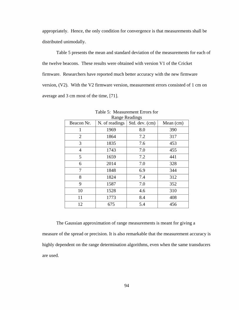
94
appropriately. Hence, the only condition for convergence is that measurements shall be
distributed unimodally.
Table 5 presents the mean and standard deviation of the measurements for each of
the twelve beacons. These results were obtained with version V1 of the Cricket
firmware. Researchers have reported much better accuracy with the new firmware
version, (V2). With the V2 firmware version, measurement errors consisted of 1 cm on
average and 3 cm most of the time, [71].
Table 5: Measurement Errors for
Range Readings Beacon Nr. N. of readings Std. dev. (cm) Mean (cm)
1 1969 8.0 390 2 1864 7.2 317 3 1835 7.6 453 4 1743 7.0 455 5 1659 7.2 441 6 2014 7.0 328 7 1848 6.9 344 8 1824 7.4 312 9 1587 7.0 352 10 1528 4.6 310 11 1773 8.4 408 12 675 5.4 456
The Gaussian approximation of range measurements is meant for giving a
measure of the spread or precision. It is also remarkable that the measurement accuracy is
highly dependent on the range determination algorithms, even when the same transducers
are used.
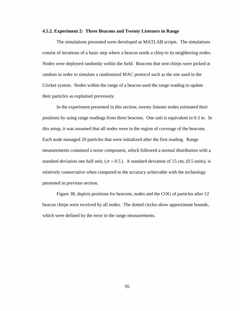
95
4.5.2. Experiment 2: Three Beacons and Twenty Listeners in Range
The simulations presented were developed as MATLAB scripts. The simulations
consist of iterations of a basic step where a beacon sends a chirp to its neighboring nodes.
Nodes were deployed randomly within the field. Beacons that sent chirps were picked at
random in order to simulate a randomized MAC protocol such as the one used in the
Cricket system. Nodes within the range of a beacon used the range reading to update
their particles as explained previously.
In the experiment presented in this section, twenty listener nodes estimated their
positions by using range readings from three beacons. One unit is equivalent to 0.3 m. In
this setup, it was assumed that all nodes were in the region of coverage of the beacons.
Each node managed 20 particles that were initialized after the first reading. Range
measurements contained a noise component, which followed a normal distribution with a
standard deviation one half unit, ( 0 5σ = . ). A standard deviation of 15 cm, (0.5 units), is
relatively conservative when compared to the accuracy achievable with the technology
presented in previous section.
Figure 38, depicts positions for beacons, nodes and the COG of particles after 12
beacon chirps were received by all nodes. The dotted circles show approximate bounds,
which were defined by the error in the range measurements.
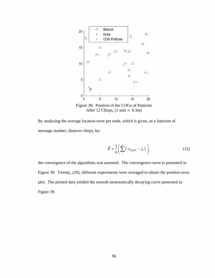
96
Figure 38: Position of the COGs of Particles
After 12 Chirps, (1 unit ≡ 0.3m) By analyzing the average location error per node, which is given, as a function of
message number, (beacon chirp), by:
TRUE1
ˆn
ii
E x xn⎛ ⎞= || − ||⎜ ⎟⎝ ⎠∑ . (12)
the convergence of the algorithms was assessed. The convergence curve is presented in
Figure 39. Twenty, (20), different experiments were averaged to obtain the position error
plot. The plotted data yielded the smooth monotonically decaying curve presented in
Figure 39.

97
Figure 39: Convergence of the Average Position Error
Figure 39 illustrates the fact that, on average, 12 beacon chirps are necessary for
achieving localization. This total number of chirps divided by the number of beacons
yields approximately 4 chirps per beacon, which is an excellent result in terms of energy
expenditure. The minimum average error was slightly higher than the standard deviation
of the measurement noise. The chirps were generated at random and the measurements
were noisy. Therefore, the number of chirps necessary was more than the minimal
number of chirps, which a complete particle filter would predict. However, it must be
reiterated that these results were obtained with only 20 particles.
4.5.3. Experiment 3: Incremental Localization
In a second experiment, the feasibility of cooperative localization using the
proposed algorithm was tested by limiting the range of the beacon chirps to a specific
distance. Therefore, listeners that were outside the range of the beacons had to wait until
nearby listeners could act as beacons. Listeners could act as beacons only after they had
localized themselves, at least partially, (incremental localization). In this experiment the
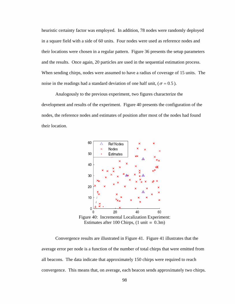
98
heuristic certainty factor was employed. In addition, 78 nodes were randomly deployed
in a square field with a side of 60 units. Four nodes were used as reference nodes and
their locations were chosen in a regular pattern. Figure 36 presents the setup parameters
and the results. Once again, 20 particles are used in the sequential estimation process.
When sending chirps, nodes were assumed to have a radius of coverage of 15 units. The
noise in the readings had a standard deviation of one half unit, ( 0 5σ = . ).
Analogously to the previous experiment, two figures characterize the
development and results of the experiment. Figure 40 presents the configuration of the
nodes, the reference nodes and estimates of position after most of the nodes had found
their location.
Figure 40: Incremental Localization Experiment:
Estimates after 100 Chirps, (1 unit ≡ 0.3m)
Convergence results are illustrated in Figure 41. Figure 41 illustrates that the
average error per node is a function of the number of total chirps that were emitted from
all beacons. The data indicate that approximately 150 chirps were required to reach
convergence. This means that, on average, each beacon sends approximately two chirps.
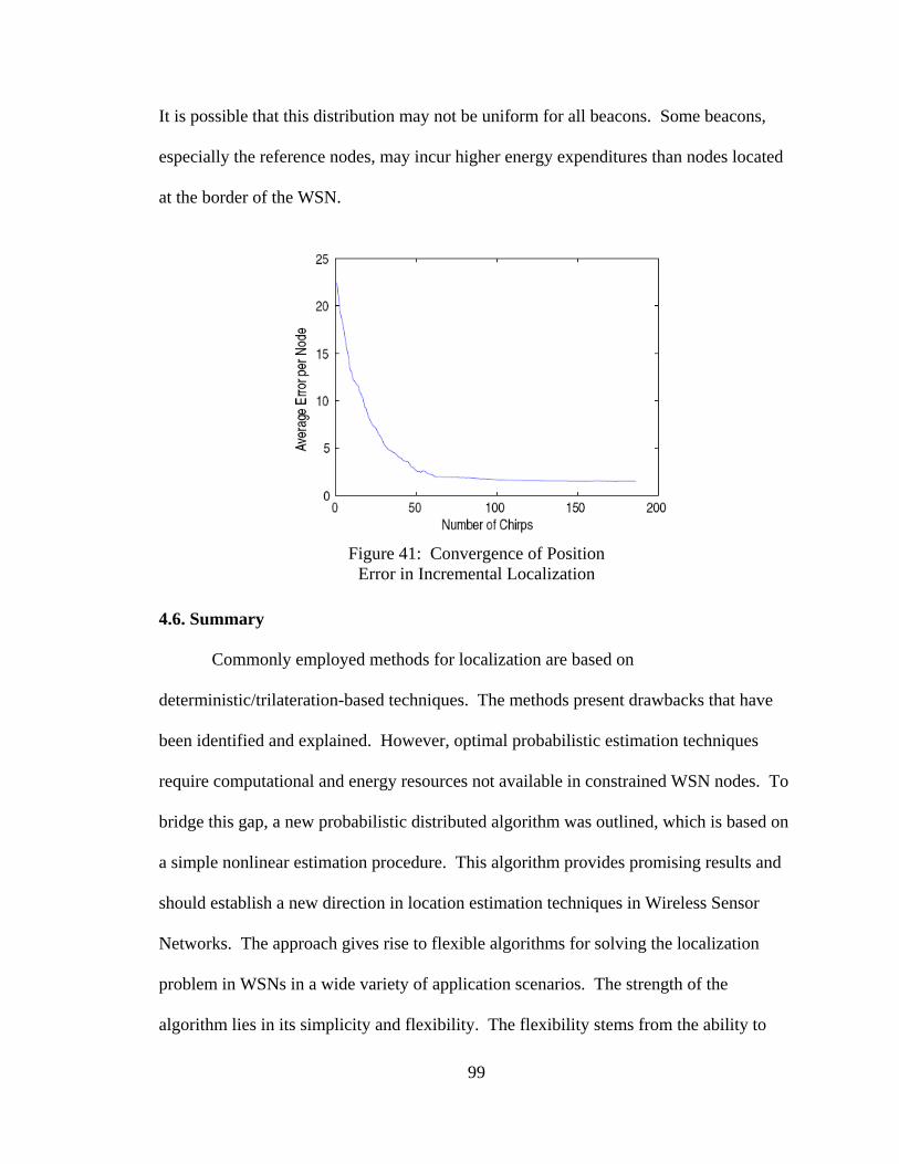
99
It is possible that this distribution may not be uniform for all beacons. Some beacons,
especially the reference nodes, may incur higher energy expenditures than nodes located
at the border of the WSN.
Figure 41: Convergence of Position
Error in Incremental Localization 4.6. Summary
Commonly employed methods for localization are based on
deterministic/trilateration-based techniques. The methods present drawbacks that have
been identified and explained. However, optimal probabilistic estimation techniques
require computational and energy resources not available in constrained WSN nodes. To
bridge this gap, a new probabilistic distributed algorithm was outlined, which is based on
a simple nonlinear estimation procedure. This algorithm provides promising results and
should establish a new direction in location estimation techniques in Wireless Sensor
Networks. The approach gives rise to flexible algorithms for solving the localization
problem in WSNs in a wide variety of application scenarios. The strength of the
algorithm lies in its simplicity and flexibility. The flexibility stems from the ability to

100
tune, using very few parameter, the convergence and accuracy of the localization process.
Given that the algorithm parameters depend on the specific application, computer
simulation studies can help in the determination of optimal values for typical scenarios.
The WSN case study helped in introducing the two main aspects of cooperative
localization and the probabilistic framework that were fundamental to this research.
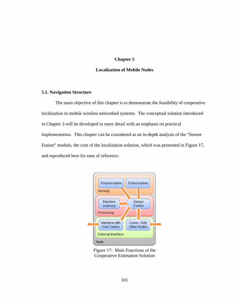
101
Chapter 5
Localization of Mobile Nodes
5.1. Navigation Structure
The main objective of this chapter is to demonstrate the feasibility of cooperative
localization in mobile wireless networked systems. The conceptual solution introduced
in Chapter 3 will be developed in more detail with an emphasis on practical
implementation. This chapter can be considered as an in-depth analysis of the “Sensor
Fusion” module, the core of the localization solution, which was presented in Figure 17,
and reproduced here for ease of reference.
Figure 17: Main Functions of the Cooperative Estimation Solution
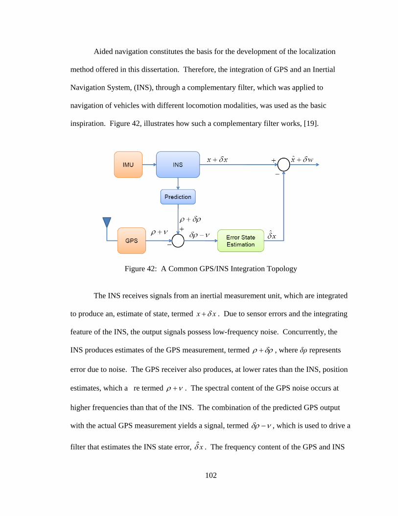
102
Aided navigation constitutes the basis for the development of the localization
method offered in this dissertation. Therefore, the integration of GPS and an Inertial
Navigation System, (INS), through a complementary filter, which was applied to
navigation of vehicles with different locomotion modalities, was used as the basic
inspiration. Figure 42, illustrates how such a complementary filter works, [19].
Figure 42: A Common GPS/INS Integration Topology
The INS receives signals from an inertial measurement unit, which are integrated
to produce an, estimate of state, termed x xδ+ . Due to sensor errors and the integrating
feature of the INS, the output signals possess low-frequency noise. Concurrently, the
INS produces estimates of the GPS measurement, termed ρ δρ+ , where δρ represents
error due to noise. The GPS receiver also produces, at lower rates than the INS, position
estimates, which a re termed ρ ν+ . The spectral content of the GPS noise occurs at
higher frequencies than that of the INS. The combination of the predicted GPS output
with the actual GPS measurement yields a signal, termed δρ ν− , which is used to drive a
filter that estimates the INS state error, ˆxδ . The frequency content of the GPS and INS

103
errors can be modeled with accuracy. Therefore, it is possible to design the error
estimation filter such that it attenuates the GPS noise while providing accurate estimates
of the INS state error. Once estimated, the error can be subtracted from the INS estimate
to yield the final state estimate, which will still possess a small residual error, termed
wδ . Variants of this method and additional details with respect to GPS/INS integration
techniques are covered in detail in, [19]. Figure 43 presents the aided navigation method
proposed in this research.
Figure 43: Proposed Structure for Aided Navigation
Figure 47 can also be attributed to the application of the functional allocation method,
which stems from the Systems Engineering approach. This navigation solution presents
three principal modules.

104
5.1.1. The INS Module
The core of the INS module consists of a filter, which performs sensor fusion of
the proprioceptive sensors. An IMU measures accelerations with a set of three
orthogonal accelerometers and measures angular rates with a set of three orthogonal
gyroscopes. The acceleration and angular rate signals, produced by the IMU, are
provided to the INS module. Most IMUs also incorporate a set of magnetometers, which
assist in initializing the INS. In addition the IMU’s magnetometer signals assist in
maintaining attitude estimates current. However, magnetometers are very sensitive to the
proximity of ferromagnetic materials, which is a major concern in their application.
The main function of the INS module is to provide optimal estimates of speed and
angular velocity, which is projected onto the configuration space of the moving node. In
addition, the INS module produces confidence parameters of a simplified motion model
operating in the configuration space, which are represented as α i in Figure 43.
Therefore, it is implicitly assumed that optimal attitude estimation is to be performed.
Due to the nonlinear nature of rigid body motion, the sensor fusion filter needs to be
realized as a nonlinear variant of an optimal estimator, which possesses the capability to
handle several states. The Extended Kalman Filter (EKF), which is proposed in this
research, represents such an optimal estimator.
The combined effect of the absence of external aids in conjunction with the non-
stationary nature of sensor errors renders estimates unusable after a relatively short period
of time. The time frame associated with usable estimates depends on the quality of the
IMU. This is the reason external updating has to be provided by the navigation aiding
module. The external updating is provided in the form of position estimates, which

105
prevent INS errors from growing without bounds. Additionally, certain techniques such
as zero updating and the incorporation of constraints in the filtering process help with
reducing the negative effects of inertial sensor errors. The machine learning function
introduced in Chapter 3 can also be considered as an add-on improvement, which was left
for future research.
5.1.2. The Navigation Aiding Module
The Navigation Aiding module is where the position estimation process is
performed. In concert with the Bayesian approach to the problem, actual estimates are
not as important as the PDF of position, which is the position belief given by, bel( )Nx .
There are several techniques for extracting an actual numeric position estimate from
belief. Subsequent section will explain how the Bayesian approach provides an elegant
way of handling uncertainty. In addition, the Bayesian approach also paves the way for
solutions that do not deal with issues related to graph rigidity. The two main
components, predication and cooperation, of a Bayesian Filter were utilized in the
navigation aiding module. Prediction was incorporated in the form of a probabilistic
motion model and in measurement updates. The probabilistic motion model was based
on velocity estimates and parameters provided by the INS module. The parameters of the
motion model are essentially a function of the measures of confidence of the velocity
estimates such as covariance or variances. Cooperation is provided by the measurement
update function. Information is provided by other nodes in the form of range
measurements, r , and reference node position belief, bel( )Lx , which are termed
collectively as “chirps.”

106
The Navigation Aiding module updates its internal predicted position belief,
which is obtained from the motion model, by using incoming chirps. The combination of
uncertain range measurements along with the position belief of the chirp originator is one
of the main topics and contributions of this dissertation, which will be presented in
Section 5.4. After the combination of these two pieces of information, the resulting PDF
is used for updating the predicted belief, which is returned to the motion model, in a
recursive procedure. The Navigation Aiding module is presented in greater detail in
subsequent sections of this chapter.
5.1.3. The Wireless Network Interface Module
The function of the Wireless Network Interface, (WNI), module is twofold. The
WNI module is used as an exteroceptive sensor for obtaining range estimates. In
addition, the WNI module is employed as a means for communication. Chirps are
generated and received by the WNI. Additionally, the WNI module directly influences
the measurement updating function of the navigation aiding module. The concrete
protocols required to handle these two aspects are elucidated in Chapter 6.
5.2. Assumptions
The structure presented in previous section has explained how sensor fusion can
yield an optimal estimate of the main states associated with the kinematics of a rigid
body. The main objective of this chapter is to present the advantages of cooperative
localization when applied to mobile nodes.
107
During the development of this section, the reader may visualize the localization
process, which takes place in a multi-robot system, as presented in Chapter 1. The
underlying assumptions, which are associated with the problem of localization presented
in this chapter, are:
• The localization problem is presented for the two-dimensional case. That is, a
mobile node in a two-dimensional plane with three degrees of freedom will be
considered. The degrees of freedom are concerned with the nodes position,
which is given by the x and y coordinates and the nodes heading, which is
represented by the angle, θ . A vector of these parameters is termed the
node’s pose, p. However, the methods proposed may be extended to three-
dimensional localization.
• Each mobile node possesses an inertial navigation system, (INS), which
receives information from six sensors. The sensors consist of three orthogonal
accelerometers and three orthogonal gyros. The INS is initialized correctly
and provides optimal estimates of horizontal linear speed, v , and angular
speed, ω . That is, the result of odometry calculations are optimal estimates
of, v , and, ω . Current pose estimates are fed-back to the INS in order to
compensate for errors inherent to inertial sensors.
• As in the case of fixed nodes, mobile nodes have the ability to exchange
“chirps”. A chirp is a signaling mechanism, which allows nodes to determine
inter-node range and to exchange belief information.
• In contrast to the problem analyzed for fixed nodes, it is assumed that there
are no restrictions with respect to energy, computational power or memory.
108
• Doppler effects due to relative motion of the mobile nodes were neglected.
• Additional errors, which may arise from lack of clock synchronization in the
process of measuring range, were neglected.
5.3. Probabilistic Motion Model
Localization can be analyzed as a hidden Markov model, (HMM). The HMM
was presented in Figure 22. In this framework, the state transition probability,
1( )t t tp x u x −| , , is determined by the motion model of the mobile node. Most of the
development in this section is based on the probabilistic methods presented in [16].
According to the decomposition presented in previous section, the state of the robot,
handled by the particle filter, is assumed to be its pose, p , which is given by:
t
t t
t
xp y
θ
⎡ ⎤⎢ ⎥⎢ ⎥⎢ ⎥⎢ ⎥⎢ ⎥⎢ ⎥⎣ ⎦
= . (13)
The inputs are the estimated translational velocity, INS tv̂ , , and rotational velocity, INS tω̂ , ,
which are provided by the INS system. The control vector, u , is comprised of the two
estimated magnitudes, which are given by:
INS tˆtv v ,= , (14)
and
INS tˆtω ω ,= . (15)
109
Thus:
tt
t
vu
ω
⎡ ⎤⎢ ⎥⎢ ⎥⎢ ⎥⎣ ⎦
= . (16)
The deterministic motion model is given by:
1 1 1
1 11
1
sin sin( )cos cos( )
t t t t t t t t t
t t t t t t tt t
tt t
x x v v ty y v v t
t
ω θ ω θ ωω θ ω θ ω
θ θ ω
⎡ ⎤ ⎡ ⎤⎢ ⎥ ⎢ ⎥− − −⎢ ⎥ ⎢ ⎥⎢ ⎥ ⎢ ⎥
− −−⎢ ⎥ ⎢ ⎥⎢ ⎥ ⎢ ⎥⎢ ⎥ ⎢ ⎥−⎣ ⎦ ⎣ ⎦
− / + / + Δ⎡ ⎤⎢ ⎥= + / − / + Δ⎢ ⎥
Δ⎢ ⎥⎣ ⎦
. (17)
In practice, the dead-reckoning process enabled by a coasting INS possesses
errors and is subject to noise and uncertainty. Therefore, the input variables can be
modeled as the estimated quantities plus a random variable, bε , with finite variance, 2b ,
and zero mean. It can be assumed that such a random variable is distributed according to
a normal distribution with parameters obtained from an error analysis of the INS system.
It has proven useful, to model the standard deviation of the noise, bε , as dependent on the
magnitude of, v , and, ω . Therefore, ut :
1 2
3 4
ˆˆ
vt t
vt t
vv α α ω
α α ω
εεωω
⎡ ⎤⎡ ⎤⎢ ⎥| |+ | |⎢ ⎥⎢ ⎥⎢ ⎥⎢ ⎥⎢ ⎥
| |+ | |⎢ ⎥⎣ ⎦ ⎣ ⎦
⎡ ⎤= +⎢ ⎥
⎣ ⎦. (18)
To obtain a complete probabilistic model of the motion of the mobile node, an
additional source of error was considered. The additional source of error results from a
random rotation after the node has moved for the discrete time interval, tΔ .
110
This error is calculated from:
5 6ˆ vα α ωγ ε | |+ | |= . (19)
The complete probabilistic motion model, (PMM), is given by:
1 1 1
1 11
1
sin sin( )ˆ ˆ ˆˆ ˆcos cos( )ˆ ˆ ˆˆ ˆ
ˆ
t t t t tt t t t
t t t t tt tt t
tt t
x x tv vy y tv v
t t
θ θω ω ωθ θω ω ω
θ θ ω γ
⎡ ⎤ ⎡ ⎤⎢ ⎥ ⎢ ⎥− − −⎢ ⎥ ⎢ ⎥⎢ ⎥ ⎢ ⎥
− −−⎢ ⎥ ⎢ ⎥⎢ ⎥ ⎢ ⎥⎢ ⎥ ⎢ ⎥−⎣ ⎦ ⎣ ⎦
− / + / + Δ⎡ ⎤⎢ ⎥= + / − / + Δ⎢ ⎥
Δ + Δ⎢ ⎥⎣ ⎦
. (20)
The noise and uncertainty, in the motion of the mobile node, depend on the
parameters, 1 2 6…α α α, , , . The larger these constants, the less accurate will be the
predictions. The growth of these constants will also be reflected in “wider” belief
distributions. These constants can be obtained from the motion model.
For particle filters, it is not necessary to compute, 1( )t t tp x u x −| , , for arbitrary tx ,
tu and 1tx − . It is sufficient to have the ability to sample from the conditional probability
density function. This will ensure that even when using identical particles for 1tx − , the
predicted values will have enough diversity before applying the measurement update.
5.3.1. Preliminary Analysis of the Probabilistic Motion Model
Several experiments were carried out to observe the effect of the parameters and
since there was no navigation aiding, the uncertainty grew. Figures 44 through 46
illustrate the overall effect of the parameters, α , for different trajectories. These results
certify that the model possesses more uncertainty with greater values of the α
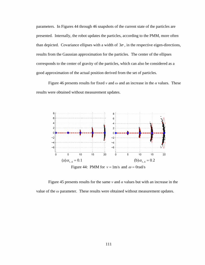
111
parameters. In Figures 44 through 46 snapshots of the current state of the particles are
presented. Internally, the robot updates the particles, according to the PMM, more often
than depicted. Covariance ellipses with a width of 3σ , in the respective eigen-directions,
results from the Gaussian approximation for the particles. The center of the ellipses
corresponds to the center of gravity of the particles, which can also be considered as a
good approximation of the actual position derived from the set of particles.
Figure 46 presents results for fixed ν and ω and an increase in the α values. These
results were obtained without measurement updates.
(a) 1 6 0 1…α = . (b) 1 6 0 2…α = .
Figure 44: PMM for 1m sv = / and 0rad sω = /
Figure 45 presents results for the same ν and α values but with an increase in the
value of the ω parameter. These results were obtained without measurement updates.

112
(a) 1 6 0 1…α = . (b) 1 6 0 2…α = .
Figure 45: PMM for 1m sv = / and 0 05rad sω = . /
Figure 46 presents results for the same ν and α values but with an increase in the
value of the ω parameter. These results were obtained without measurement updates.
(a) 1 6 0 1…α = . (b) 1 6 0 2…α = .
Figure 46: PMM for 1m sv = / and [0 1( 10) ( 0 1)( 10)]rad st tω = . < + − . ≥ /
The effect of the individual α parameters is presented in Figures 47 through 49
using similar conditions to those presented in Figure 44. These results indicate that the
model is highly sensitive to the parameters, which define the uncertainty in rotational
motion, ( 3 6…α α ). However, the uncertainty in the translational velocity, ( 1 2α α, ), does
not produce any significant spread in the belief. Figure 47 presents the results obtained

113
for an increase in the uncertainty in the ν parameter but with fixed values for the α
parameters.
Figure 47: PMM with Greater Uncertainty in v :
1 2 0 5α , = . , 3 4 5 6 0 05α , , , = .
Figure 48 presents the results obtained for an increase in the uncertainty in the ω
parameter but with fixed values for the α parameters.
Figure 48: PMM with Greater Uncertainty inω :
3 4 0 5α , = . , 1 2 5 6 0 05α , , , = .
Figure 49 presents the results obtained for an increase in the uncertainty in the γ
parameter but with fixed values for the α parameters.

114
Figure 49: PMM with Greater Uncertainty in γ :
5 6 0 5α , = . , 1 2 3 4 0 05α , , , = .
It is also indicated that the distributions of the belief, after the prediction, are not
Gaussian. Therefore, particle filters offer a very appropriate way to represent belief.
With growing uncertainty, greater spread, in the position of the robot, is expected
since it is only subject to prediction through dead-reckoning. Table 6 summarizes the
results of these preliminary experiments. The maximum error and spread, ( 3σ ), of the
particles was produced at the end of the experiment. Both values are presented in the last
column of Table 6.
Table 6: Quantitative Results of Experiments
With the Motion Model Trajectory 1α , 2α 3α , 4α 5α , 6α MAX3σ (m) Error (m)
Straight Line 0.10 0.10 0.10 3.20 0.04 Straight Line 0.20 0.20 0.20 6.35 0.17 Straight Line 0.50 0.05 0.05 1.60 0.01 Straight Line 0.05 0.50 0.05 10.6 0.49 Straight Line 0.05 0.05 0.50 11.0 0.53
Curve 0.10 0.10 0.10 3.26 0.05 Curve 0.20 0.20 0.20 6.46 0.18
S-Shaped 0.10 0.10 0.10 3.38 0.06 S-Shaped 0.20 0.20 0.20 6.69 0.20

115
5.3.2. Basic Navigation Aiding
In particle filtering, the measurement update is performed through computation of
the weight of the particles and through the resampling procedure. The weight of the
particles is given by:
[ ] [ ]( )m mt t tw p z x= | . (21)
In this specific example, it was assumed that the moving node can measure its distance to
reference nodes with known positions. Since the experiment was preliminary, the
position of the reference nodes was assumed to be known with perfect certainty. In latter
sections, the uncertainty in the positions of the reference nodes will be taken into account.
The uncertainty of the reference nodes had to be taken into account since other mobile
nodes become reference nodes for the mobile node, which is to be localized.
Range measurements were assumed to possess normally distributed noise with a
specific standard deviation. The standard deviation was chosen so that the associated
probability density function, ( )t tp z x| , would resemble the curve presented in Figure 50.
The PDF presented in Figure 50 is for a “beacon”, reference node, located at, (8m, 8m).
In the illustrated example, the measured range was 5m and the standard deviation was
1m.
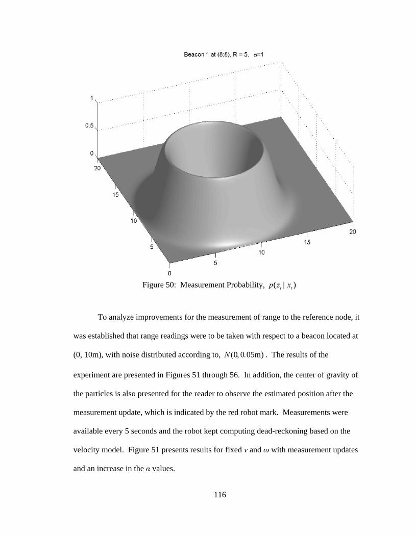
116
Figure 50: Measurement Probability, ( )t tp z x|
To analyze improvements for the measurement of range to the reference node, it
was established that range readings were to be taken with respect to a beacon located at
(0, 10m), with noise distributed according to, (0 0 05m)N , . . The results of the
experiment are presented in Figures 51 through 56. In addition, the center of gravity of
the particles is also presented for the reader to observe the estimated position after the
measurement update, which is indicated by the red robot mark. Measurements were
available every 5 seconds and the robot kept computing dead-reckoning based on the
velocity model. Figure 51 presents results for fixed ν and ω with measurement updates
and an increase in the α values.

117
(a) 1 6 0 1…α = . (b) 1 6 0 2…α = .
Figure 51: PMM for 1m sv = / and 0rad sω = / with Measurement Updates
Figures 51 and 44 should be compared since they present results for different
experiments with the same parameter values. Figure 52 presents, with measurement
updates, results for the same ν and α values but with an increase in the value of the ω
parameter.
(a) 1 6 0 1…α = . (b) 1 6 0 2…α = .
Figure 52: PMM for 1m sv = / and 0 05rad sω = . / with Measurement Updates

118
Figures 52 and 45 should be compared since they present results for different
experiments with the same parameter values. Figure 53 presents, with measurement
updates, results for the fixed ν and α values but with a varying value ω parameter.
(a) 1 6 0 1…α = . (b) 1 6 0 2…α = .
Figure 53: PMM for 1m sv = / and Varying ω with Measurement Updates
Figures 53 and 46 should be compared since they present results for different
experiments with the same parameter values. Figure 54 presents results for an increased
uncertainty in the ν parameter with measurement updates.
Figure 54: PMM with Greater Uncertainty in
v With Measurement Updates

119
Figures 54 and 47 should be compared since they present results for experiments
with and without measurement updates but with increased uncertainty in the ν parameter.
Figure 55 presents results for an increased uncertainty in the ω parameter with
measurement updates.
Figure 55: PMM with Greater Uncertainty in
ω With Measurement Updates
Figures 55 and 48 should be compared since they present results for experiments
with and without measurement updates but with increased uncertainty in the ω parameter.
Figure 56 presents results for an increased uncertainty in the γ parameter with
measurement updates.
Figure 56: PMM with Greater Uncertainty in
γ With Measurement Updates

120
Figures 56 and 49 should be compared since they present results for experiments
with and without measurement updates but with increased uncertainty in the γ parameter.
In all cases, even though the measurements were noisy, the uncertainty was
reduced due to the measurements obtained from the reference node. It is also indicated
that if measurements were available more often, the divergence of the particles would be
much reduced. Another way to reduce divergence would be to have reference nodes
located at different places in order to yield a trilateration-like effect. In such a situation
the robot would keep the spread of the location belief within bounds. Table 7
summarizes the experiments considering the measurement update. For comparison
purposes, the results listed in Table 6 have also been included.
Table7: Quantitative Results of Experiments with the
Motion Model and Range Measurements w. Range
Meas. w.o. Range
Meas. Trajectory 1α , 2α 3α , 4α 5α , 6α MAX3σ
(m)
Δ (m)
MAX3σ
(m)
Δ (m)
Straight Line 0.10 0.10 0.10 1.05 0.04 3.20 0.04 Straight Line 0.20 0.20 0.20 2.38 0.12 6.35 0.17 Straight Line 0.50 0.05 0.05 0.96 0.05 1.60 0.01 Straight Line 0.05 0.50 0.05 3.36 0.27 10.6 0.49 Straight Line 0.05 0.05 0.50 3.70 0.30 11.0 0.53
Curve 0.10 0.10 0.10 1.14 0.07 3.26 0.05 Curve 0.20 0.20 0.20 2.01 0.09 6.46 0.18
S-Shaped 0.10 0.10 0.10 1.20 0.05 3.38 0.06 S-Shaped 0.20 0.20 0.20 2.23 0.13 6.69 0.20
121
5.4. Measurement Update with Respect to Non-Deterministic Reference Nodes
In section 5.3, the positive effect of range measurements on the position belief
was presented. The position of the reference node was assumed to be known with perfect
certainty. In this section, this assumption is relaxed. In order to gain insight into the
problem, the analysis will be reduced to the one-dimensional case. That is, nodes are
only allowed to move along the, x , direction. However, initially, distributions are not
assumed to follow a Gaussian distribution. The range measurement is a random variable,
R , given by the probability density function:
( ) ( )Rf r p z x= | , (22)
with the corresponding cumulative distribution, ( )RF r , given by:
{ ( ]} ( ) ( )a
R RP R a F a f r dr−∞
∈ −∞, = = ∫ . (23)
Analogously, the position of the reference node is a random variable, L , given by
its belief, bel( )Lx , which is a probability density function, ( )Lf l , with its respective
cumulative distribution, ( )LF l , which is given by:
{ ( ]} ( ) ( )b
L LP L b F b f x dx−∞
∈ −∞, = = ∫ . (24)
Using these two distributions, equations 23 and 24, the distribution for the
measurement update is sought, given that the reference node is no longer a set of
numbers. Instead the reference node is a belief. Therefore, the PDF of P is sought from:
122
( ) ( bel( ) )P Lf x p z x x= , | . (25)
These three variables P, L and R are related geometrically by:
P L R= + . (26)
The cumulative distribution function of P satisfies:
( ) ( ) ( ) ( )P L R R Ll r xF x F x f r f l dr dl+ + ≤
= = ∫∫ . (27)
This expression may be manipulated to obtain a definitive expression given by:
( )( ) ( ) ( )
( ) ( )
( ) ( )
x l
L R R L
x l
R L
R L
F x f r f x dr dl
f r dr f l dl
F x l f l dl
∞ −
+ −∞ −∞
∞ −
−∞ −∞
∞
−∞
=
=
= −
∫ ∫
∫ ∫
∫
. (28)
To obtain ( )Pf x , equation 28 may be differentiated, which yields:
[ ]
( ) ( ) ( )
( ) ( )
( ) ( )
( ) ( ) ( )
P L R R L
R L
R L
P R L
df x f x F x l f dldx
d F x l f l dldx
f x l f l dl
f x f x f x
∞
+ −∞
∞
−∞
∞
−∞
= = −
= −
= −
= ∗
∫
∫
∫
. (29)

123
Equation 29 states that the resulting PDF for P is the convolution of the individual
PDFs for R and L. This result is corroborated in the statistical literature; for instance,
[72]. The PDF for measurement updates, which is given by equation 25, can be rewritten
as:
( bel( ) ) bel( )L Lp z x x x R, | = ∗ . (30)
5.4.1. Gaussian Measurement: Uniform Landmark Position
The previous results obtained will be applied to a concrete example in this
section. In the example, the distance measurement from the position of node, Np , to the
nominal position of the reference node, Lp , is distributed according to:
(15 1)N Lr p p N= − ,∼ . (31)
The PDF of the reference node is given by:
0 1 ( 5 5)0 otherwiseL
xp
. ∈ − ,⎧= ⎨⎩
(32)
The resulting PDF for the position of the node to be localized is given by:
N Lp p r= ∗ . (33)
Figure 57 presents the three distributions pictorially.
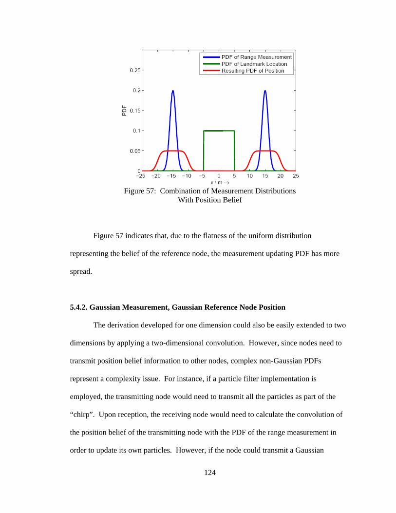
124
Figure 57: Combination of Measurement Distributions
With Position Belief
Figure 57 indicates that, due to the flatness of the uniform distribution
representing the belief of the reference node, the measurement updating PDF has more
spread.
5.4.2. Gaussian Measurement, Gaussian Reference Node Position
The derivation developed for one dimension could also be easily extended to two
dimensions by applying a two-dimensional convolution. However, since nodes need to
transmit position belief information to other nodes, complex non-Gaussian PDFs
represent a complexity issue. For instance, if a particle filter implementation is
employed, the transmitting node would need to transmit all the particles as part of the
“chirp”. Upon reception, the receiving node would need to calculate the convolution of
the position belief of the transmitting node with the PDF of the range measurement in
order to update its own particles. However, if the node could transmit a Gaussian
125
approximation of belief, less parameters would be required. In addition, the fact that a
Gaussian is obtained from the convolution of two Gaussian could be also exploited.
It can be easily shown that if the range measurement, ( )m mN r σ, , and the position
belief of the reference node, ( )L LN μ σ, , are distributed normally, the resulting PDF is
also Gaussian, ( )N NN μ σ, . The standard deviation of the new Gaussian can be
determined from:
2 2
N N Lσ σ σ= + . (34)
This relationship, given by equation 34, was applied in order to simplify the
method for computing the convolution of a Gaussian range measurement in the two-
dimensional case. In the two dimensional case the range measurement possesses a
bivariate Gaussian belief of position of the reference node. This convolution was handled
in polar coordinates, where all random variables are normally distributed.
The position belief of the reference node, bel( )Lx , is described by a Gaussian
bivariate distribution with mean vector, Lμ , and covariance matrix, LΣ , and is given as:
bel( ) ( )L L LN μ ,Σx ∼ . (35)
The range measurement is given by:
|| || ( )N L m mr N r σ= − ,x x ∼ . (36)

126
The distribution is sought, which will be applied for weighting the belief of a node using
the range measurement, for localization. The required distribution is given by:
( bel( ) ) ( )N Rp r f, | =Lx x x . (37)
The covariance matrix, LΣ , can be decomposed into its eigenvectors and eigenvalues
such that:
L λΣ =v v . (38)
Therefore, unitary eigenvectors 1v and 2v are obtained with corresponding eigenvalues
1λ and 2λ . A unit vector can also be obtained from the mean to an arbitrary point, which
is given by:
L
L
μμ
−=
−xux
. (39)
The angle θ between u and the eigenvector 1v can be calculated from:
1cos( )θ = ⋅u v , (40)
and since 1v and 2v are orthogonal, sin( )θ can be obtained from:
1sin( )θ = ⋅u v . (41)
127
Using equation 34, equation 40 and equation 41, the new variance for any given angle θ
can be computed from:
2 2
2 2 1 22 2 2 22 1 1 2
( )( ) ( )m
λ λσ θ σλ λ
= +⋅ + ⋅u v u v
. (42)
The probability as a function of angle and distance can then be computed from the
Gaussian distribution and is given by:
22
( bel( ) ) ( || ||)
1 1exp (|| || )2( ( ))2 ( )
N R L
L m
p r f
r
θ μ
μσ θπσ θ
⎛ ⎞⎜ ⎟⎜ ⎟⎜ ⎟⎝ ⎠
, | = , −
= − − −
Lx x x
x (43)
This analysis, equations 34 through 43, was applied to the computation of the distribution
of the measurement update for the specific case where the position belief of the reference
node was given by:
0 4 1
bel( )0 1 1L
⎛ ⎞⎡ ⎤ ⎡ ⎤,⎜ ⎟⎢ ⎥ ⎢ ⎥
⎣ ⎦ ⎣ ⎦⎝ ⎠x ∼ , (44)
and the range measurement was given by:
(15 1)r N ,∼ . (45)
Figure 58 presents the results for the position belief of the reference node.

128
Figure 58: Position Belief of the Reference Node
Figure 59 presents the results for PDF of the measurement update distribution without
considering the position uncertainty of the reference node.
Figure 59: PDF of the Range Measurement
Figure 60 presents the results for the PDF of the convolved distribution.
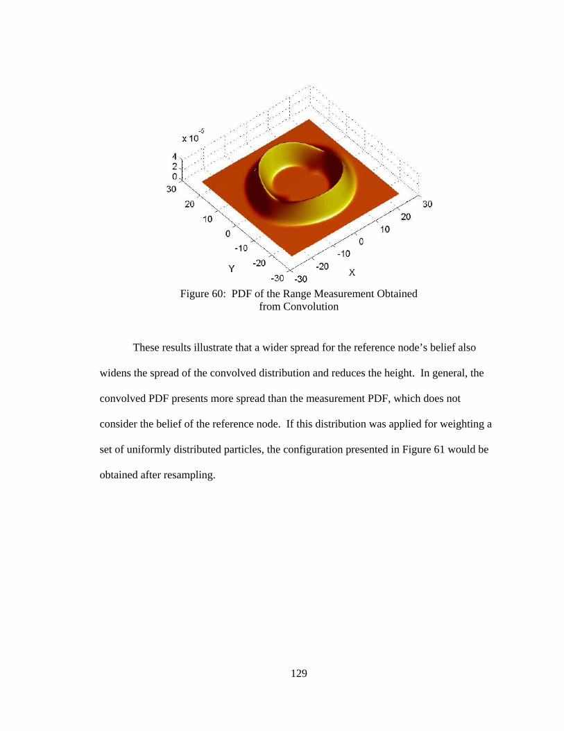
129
Figure 60: PDF of the Range Measurement Obtained
from Convolution
These results illustrate that a wider spread for the reference node’s belief also
widens the spread of the convolved distribution and reduces the height. In general, the
convolved PDF presents more spread than the measurement PDF, which does not
consider the belief of the reference node. If this distribution was applied for weighting a
set of uniformly distributed particles, the configuration presented in Figure 61 would be
obtained after resampling.

130
Figure 61: Belief after Applying a Measurement
Update with a Convolved PDF
5.5. Experiments in Cooperative Localization
In order to isolate the estimation aspect from the protocols required for
localization, in all the examples studied in this section, perfect networking was assumed.
Nodes were able to exchange chirps simultaneously at specified time intervals. Nodes
were not required to contend with medium access conflicts or the establishment of
networking links. However, the limitations of ranging technology were taken into
account. Therefore, chirps could not be transmitted to nodes that were beyond the
coverage area for ranging.
5.5.1. Cooperative Localization of Two “Passing-By” Nodes
In this experiment, two nodes moved towards one another. Both nodes
maintained the same speed. For comparison purposes, the experiment was conducted
with and without cooperation. When the nodes cooperated, chirps were exchanged every,
chirp 5T = s.
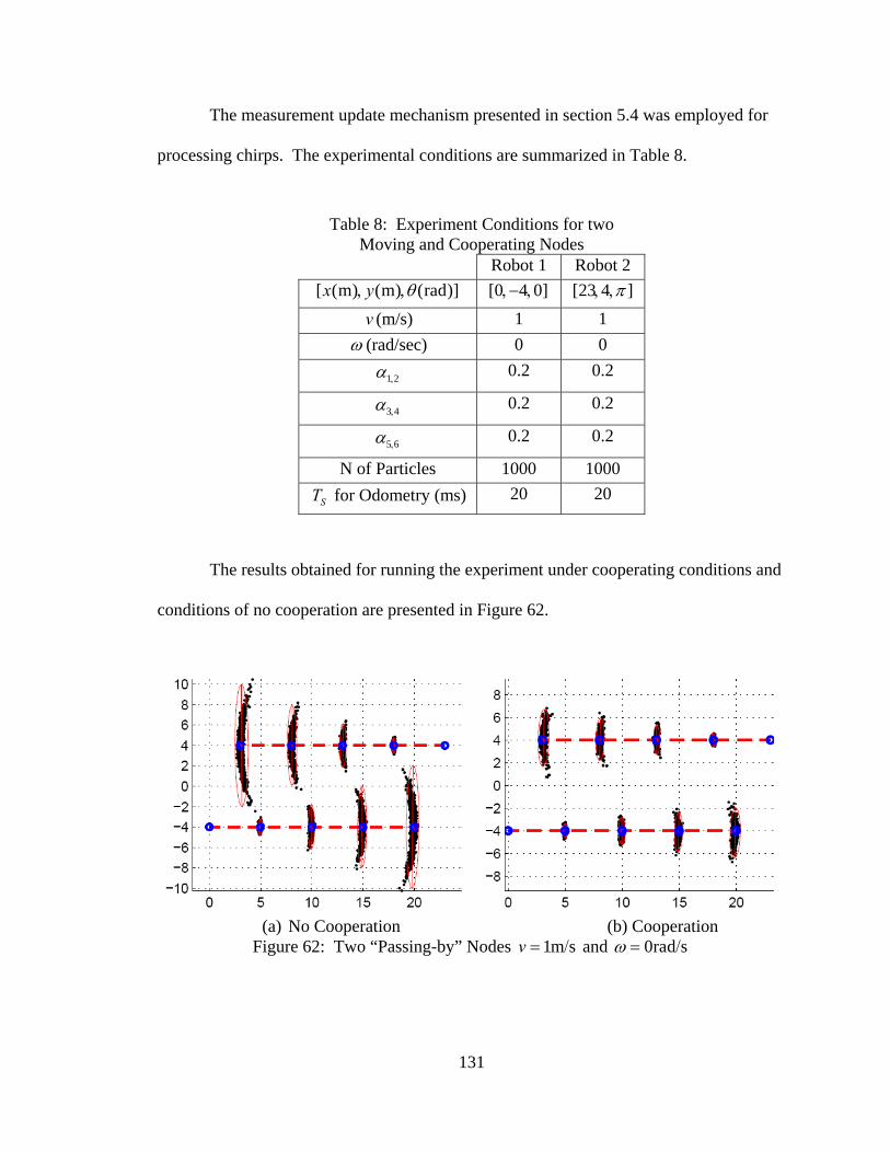
131
The measurement update mechanism presented in section 5.4 was employed for
processing chirps. The experimental conditions are summarized in Table 8.
Table 8: Experiment Conditions for two
Moving and Cooperating Nodes Robot 1 Robot 2
[ (m) (m) (rad)]x y θ, , [0 4 0], − , [23 4 ]π, , v (m/s) 1 1
ω (rad/sec) 0 0
1 2α , 0.2 0.2
3 4α , 0.2 0.2
5 6α , 0.2 0.2
N of Particles 1000 1000
ST for Odometry (ms) 20 20
The results obtained for running the experiment under cooperating conditions and
conditions of no cooperation are presented in Figure 62.
(a) No Cooperation (b) Cooperation
Figure 62: Two “Passing-by” Nodes 1m sv = / and 0rad sω = /

132
Numerical results for experiments involving no cooperation, cooperation with of
the other moving node and cooperation with a fixed reference node are presented in Table
9. The results for only one of the nodes are presented, since the results for both nodes
were very similar.
Table 9: Experimental Results Showing the Effect of Cooperation and no Cooperation for a Mobile Node
No Cooperation
Cooperation w Moving Node
Cooperation with Fixed Node
3 MAXσ Δ 3 MAXσ Δ 3 MAXσ Δ
6.05m 0.17m 2.53m 0.15m 2.38m 0.12m
5.5.2. Cooperative Localization of a Robot Swarm Moving in Formation
The goal of this experiment was to demonstrate the effect of cooperative
localization for a swarm of robots. The robot team consisted of four robots, which
moved in a square-shaped formation. The formation of the swarm is presented in Figure
63.
Figure 63: Robots moving in a Square-Shaped Formation

133
The algorithms required to build such a formation are beyond the scope of this
analysis. The robots used pre-computed controls, which allowed them to maintain the
formation. The conditions of the experiment are presented succinctly in Table 10 and are
similar to the conditions presented in Figures 46 and 53 where one node followed an s-
shaped trajectory.
Table 10: Experimental Conditions for Localization of a Robot Swarm
Robot 1 Robot 2 Robot 3 Robot 4 [ (m) (m) (rad)]x y θ, , [4 1 0], , [0 1 0], − , [1 2 0], , [3 2 0], − ,
v (m/s) 1 1 1 1 ω (rad/sec) 0.1,-0.1 0.1,-0.1 0.1,-0.1 0.1,-0.1
1 2α , 0.2 0.2 0.2 0.2
3 4α , 0.2 0.2 0.2 0.2
5 6α , 0.2 0.2 0.2 0.2
N. of Particles 1000 1000 1000 1000
ST for Odometry (ms) 20 20 20 20
Tc for Chirps (s) 5 5 5 5
Figure 64 depicts snapshots of the particles, of each robot every five seconds,
while traversing the s-shaped path. The actual results are presented in Table 11. Table
11 contains results for unaided and reference-node-aided localization for purposes of
comparison.
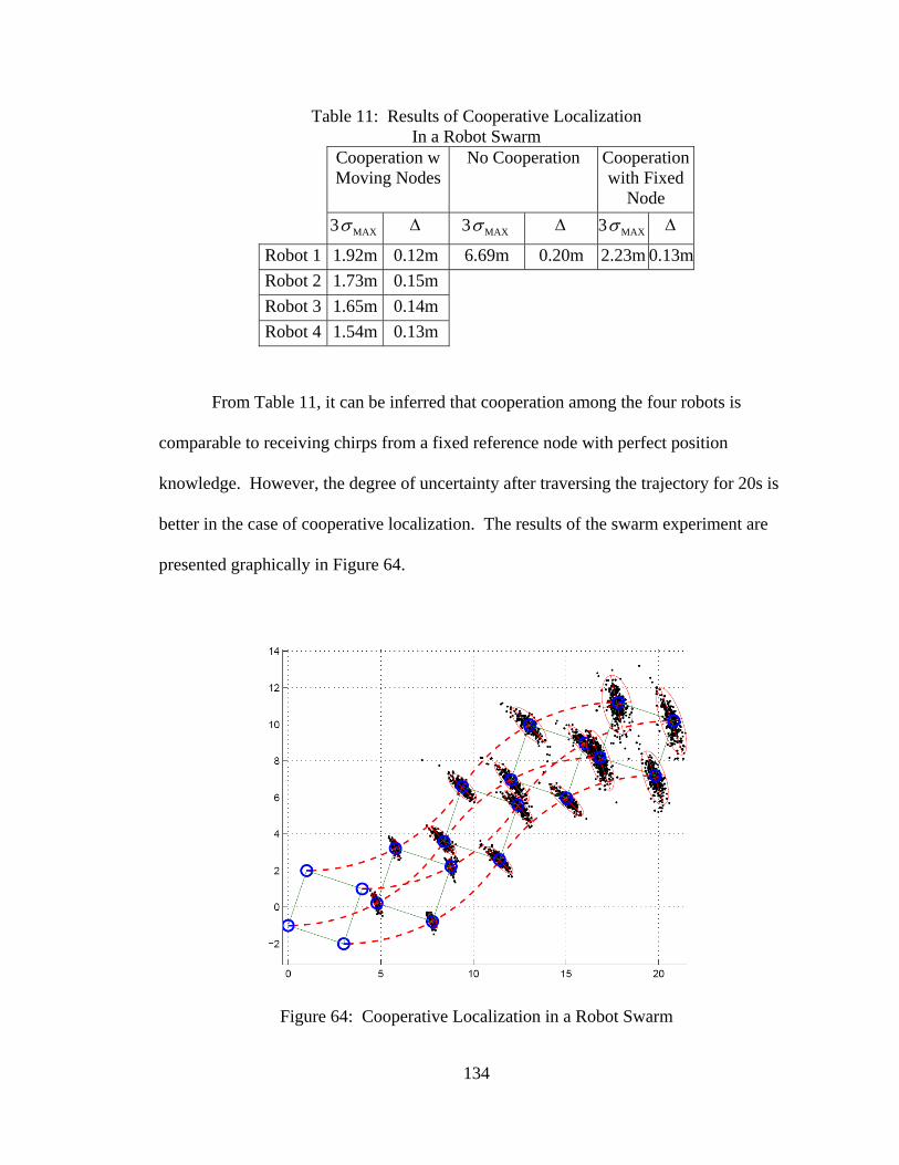
134
Table 11: Results of Cooperative Localization In a Robot Swarm
Cooperation w Moving Nodes
No Cooperation Cooperation with Fixed
Node 3 MAXσ Δ 3 MAXσ Δ 3 MAXσ Δ
Robot 1 1.92m 0.12m 6.69m 0.20m 2.23m 0.13m Robot 2 1.73m 0.15m Robot 3 1.65m 0.14m Robot 4 1.54m 0.13m
From Table 11, it can be inferred that cooperation among the four robots is
comparable to receiving chirps from a fixed reference node with perfect position
knowledge. However, the degree of uncertainty after traversing the trajectory for 20s is
better in the case of cooperative localization. The results of the swarm experiment are
presented graphically in Figure 64.
Figure 64: Cooperative Localization in a Robot Swarm

135
5.6. Summary
This chapter has presented the principal results and contributions of this
dissertation, which are:
• A novel navigation principle, which integrates an INS with range readings
for cooperative localization. The navigation principle is based on particle
filtering techniques and a probabilistic motion model,
• A detailed development of the conceptual notion of “chirp” in cooperative
localization,
• The measurement update from a reference node with a given position
belief was found to be equal to the convolution of the measurement PDF
with the PDF of the belief,
• A simplified, exact, algorithm for computing the convolution of the
measurement PDF with the PDF of the belief. The convolution is specific
to the case when range measurement noise and the position belief of the
reference node can be assumed to be Gaussian,
• Several experimental scenarios, where the usefulness of the cooperative
localization techniques, were highlighted.

136
Chapter 6
The Role of Protocols
In this chapter, the exchange of chirps will be investigated in more detail. Some
of the assumptions made in previous chapters will be relaxed. Communication protocols
provide for efficient medium utilization, for the creation of communication links and for
establishing paths for packet delivery. In a similar way, localization protocols provide
for efficient and fair swapping of chirps among nodes, which are to be localized.
The main goal of the networking function in a wireless networked system is to
transmit data. The transmitted data is not simply limited to that used for localization.
The transmission of operational data related to the mission of the WSN is paramount.
Therefore, in cases when the localization function shares the wireless network interfaces,
(WNI), with the main data transmission function, it cannot have higher priority.
Therefore, the localization function needs to use the WNI sparingly, which forces a
careful design of the localization protocols.
Localization protocols deal mainly with the two lower layers of the OSI model of
networking. The layers associated with cooperative localization are presented in Figure
65.
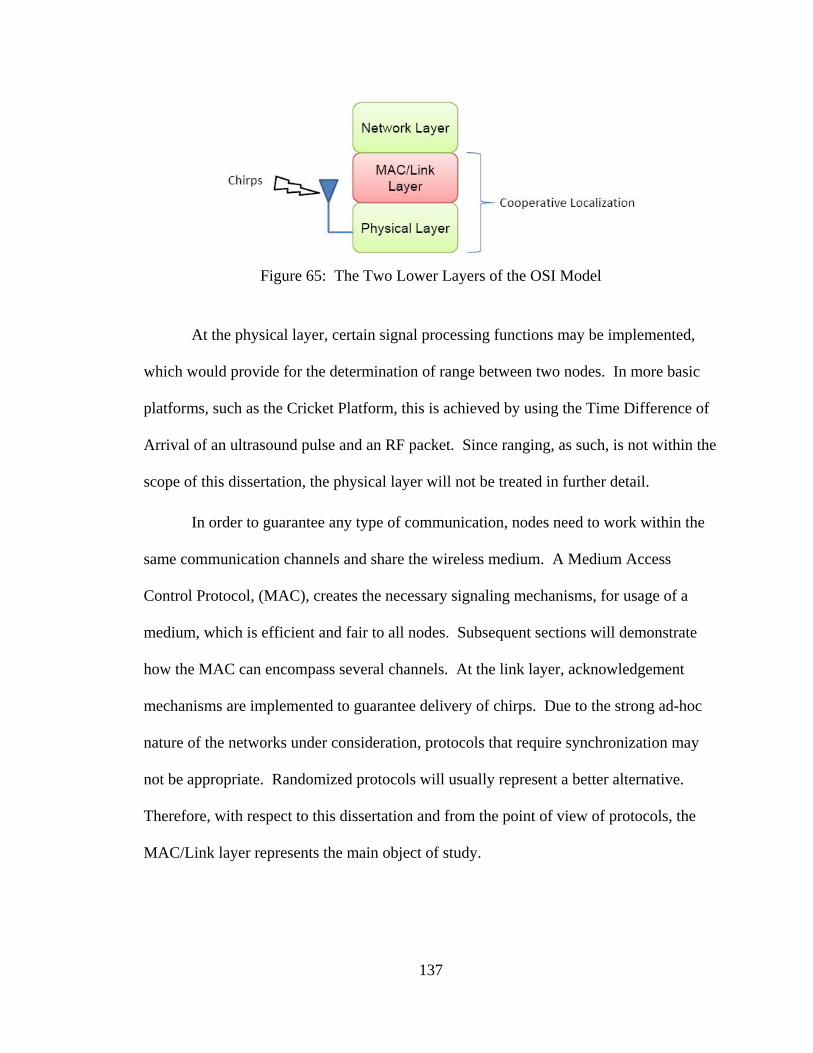
137
Figure 65: The Two Lower Layers of the OSI Model
At the physical layer, certain signal processing functions may be implemented,
which would provide for the determination of range between two nodes. In more basic
platforms, such as the Cricket Platform, this is achieved by using the Time Difference of
Arrival of an ultrasound pulse and an RF packet. Since ranging, as such, is not within the
scope of this dissertation, the physical layer will not be treated in further detail.
In order to guarantee any type of communication, nodes need to work within the
same communication channels and share the wireless medium. A Medium Access
Control Protocol, (MAC), creates the necessary signaling mechanisms, for usage of a
medium, which is efficient and fair to all nodes. Subsequent sections will demonstrate
how the MAC can encompass several channels. At the link layer, acknowledgement
mechanisms are implemented to guarantee delivery of chirps. Due to the strong ad-hoc
nature of the networks under consideration, protocols that require synchronization may
not be appropriate. Randomized protocols will usually represent a better alternative.
Therefore, with respect to this dissertation and from the point of view of protocols, the
MAC/Link layer represents the main object of study.

138
6.1. The Cricket Platform
The Cricket localization system, which was developed at MIT and
commercialized by the Crossbow Company, constitutes and ideal platform for
investigating the issues related to protocols. The main advantage of the Cricket system is
that it is based on the TinyOS operating system. The TinyOS operating system is widely
popular, open-source and targeted to Wireless Sensor Networks. TinyOS provides
abstractions that allow for the selective customization of specific functions within the
package of functions available. In this research TinyOS was particularly suitable since it
provided for the notion of a chirp to be embodied in a very direct manner.
6.1.1. Cricket V2.0 Protocol
A chirp, in the Cricket system, comprises an ultrasound pulse and an RF packet
with the position information of the transmitting node. Therefore, a chirp requires an
ultrasound channel and a RF channel. Nodes cannot transmit ultrasound pulses
simultaneously since such activity would create a collision. The receivers would not be
able to determine the source of the chirp from the signal mixture. The situation is
resolved by employing the Carrier Sense Multiple Access, (CSMA), technique. In
CSMA, a node uses its ultrasound receiver to detect whether other nodes are transmitting.
In case a signal is detected, the node waits for a random time, which is termed random
back-off, before attempting a transmission. A similar mechanism is employed for the
RF-channel.
The, off-the-shelf, Cricket localization function possesses modes for transmitting
and receiving. The transmitting mode is termed “beacon” and the receiving mode is

139
termed “listener”. Nodes may be set to work in only one mode. Therefore, nodes can be
setup to be beacons or listeners but not both at the same time. Beacons are placed at
known positions, which means that they do not perform any localization activities.
However, listeners use chirps from beacons to find their location via trilateration.
Figure 66 presents a graphical representation, component diagram, of the main
Cricket V2.0 software configuration, which details all of its main components.
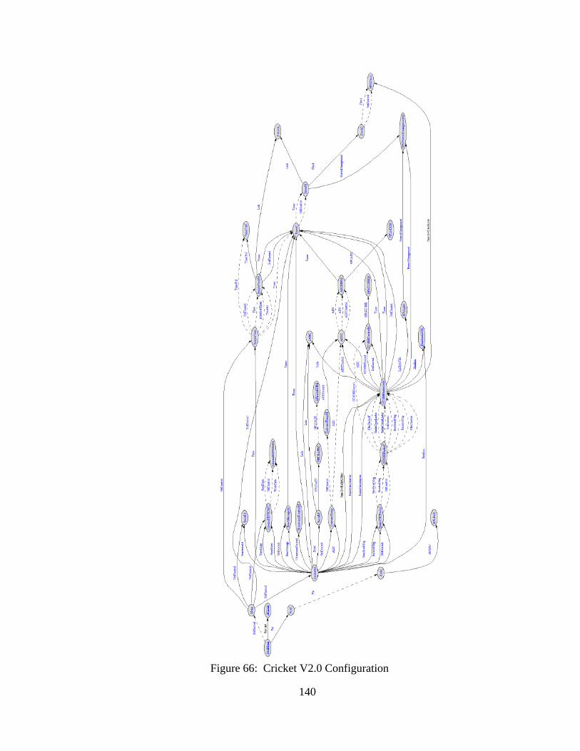
140
Figure 66: Cricket V2.0 Configuration
141
In Figure 66, the UltrasoundControlM module performs the function of
controlling the ultrasound channel by providing the UltrasoundControl interface.
The UltrasoundControl interface is comprised of several commands and events
such as:
• command result_t UltrasoundControl.StartDetector,
• command result_t UltrasoundControl.StopDetector,
• event result_t UltrasoundControl.PulseDetected,
• event result_t UltrasoundControl.DetectorTimeout,
• command result_t UltrasoundControl.SendPulse,
• command result_t UltrasoundControl.SetGain.
Control of the RF channel is analyzed in a similar manner. The RF channel
contains the CC1000RadioIntM module. The CC1000RadioIntM module provides
several interfaces for setting a node to either the listening mode or the receiving mode. In
addition, the CC1000RadioIntM module possesses capabilities for receiving and
transmitting messages.
The protocols for the, off-the-shelf, Cricket V2.0 application are depicted, in simplified
form, in Figure 67.
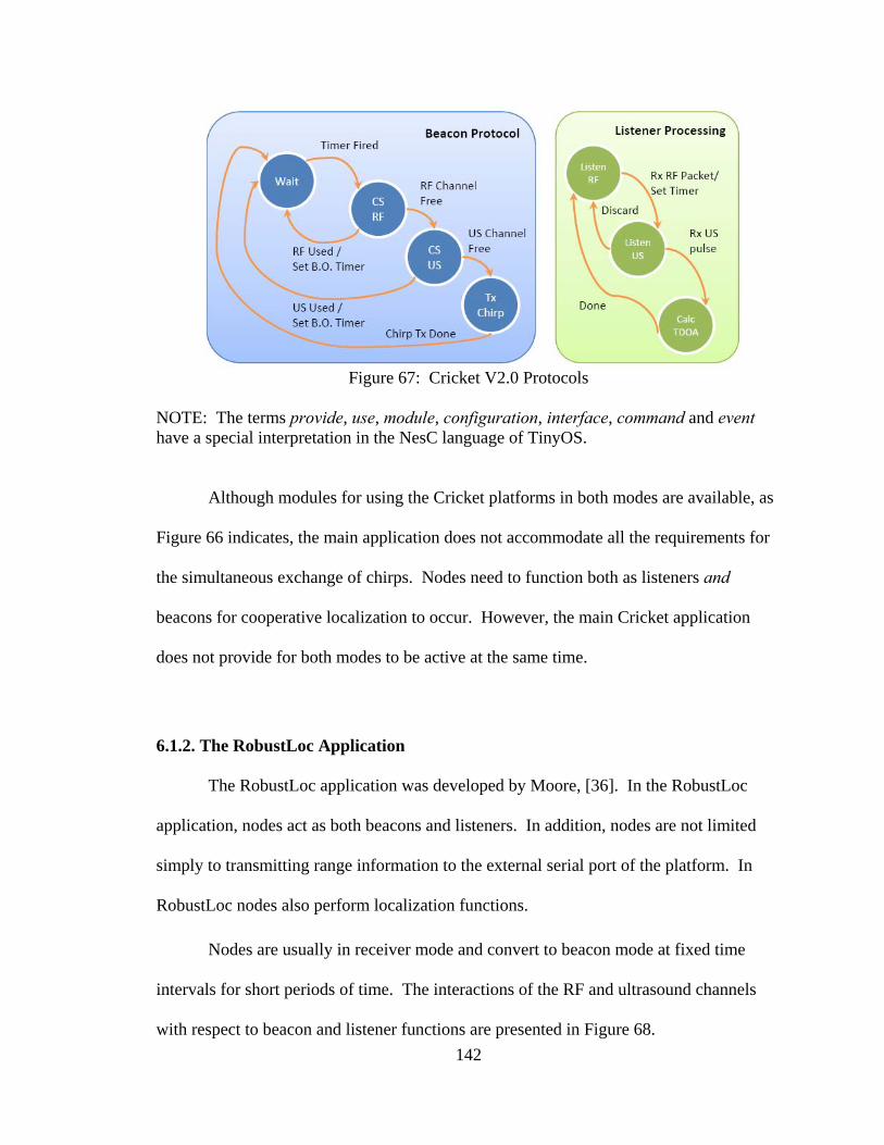
142
Figure 67: Cricket V2.0 Protocols
NOTE: The terms provide, use, module, configuration, interface, command and event have a special interpretation in the NesC language of TinyOS.
Although modules for using the Cricket platforms in both modes are available, as
Figure 66 indicates, the main application does not accommodate all the requirements for
the simultaneous exchange of chirps. Nodes need to function both as listeners and
beacons for cooperative localization to occur. However, the main Cricket application
does not provide for both modes to be active at the same time.
6.1.2. The RobustLoc Application
The RobustLoc application was developed by Moore, [36]. In the RobustLoc
application, nodes act as both beacons and listeners. In addition, nodes are not limited
simply to transmitting range information to the external serial port of the platform. In
RobustLoc nodes also perform localization functions.
Nodes are usually in receiver mode and convert to beacon mode at fixed time
intervals for short periods of time. The interactions of the RF and ultrasound channels
with respect to beacon and listener functions are presented in Figure 68.

143
Figure 68: RobustLoc Protocol
6.2. Chirp Reception Frequency
The effort to maintain odometry errors within prescribed bounds is substantially
reduced at higher frequencies. Therefore, the integrated navigation perspective considers
higher frequency navigation aids as superior. However, medium allocation is not
instantaneous. A definitive time is required to transmit chirps. Thus, the frequency at
which nodes receive chirps is an important metric that measures the efficiency of the
protocol.
The goal in this section is to develop the nature of the chirp reception process
from the statistical perspective. The distribution of the range errors for this specific
technology was scrutinized in section 4.5.1. Instead of modeling the protocols
theoretically, an empirical model is sought. The model can later be incorporated into the
navigation and motion models, which provides for a more realistic prediction functions
such as accuracy and latency.

144
In pursuit of this objective, the question is posed:
• Assuming a network of n nodes, with every node having the ability to see
all the others, what maximum chirp rate is achievable?
A perfect Time Division Multiple Access, (TDMA), protocol can be taken as an
ideal case, which may yield the highest possible chirp rate. Two channels, ultrasound
and RF, are shared by Cricket nodes. The channel, which defines the maximum chirp
frequency, is the ultrasound channel since it operates in the slower medium. The
maximum range of the Cricket ultrasound transducer was found to be approximately 5m.
Therefore, each chirp allocates the ultrasound medium for at least a time, which is given
by:
Sound
5 15ms340m s
r mtv
Δ = = =/
. (46)
If nodes would take turns in a highly synchronized manner, they would need to
wait to use the channel for a time given by:
T n tΔ = Δ . (47)
For a network with 6n = , this represents a waiting time of 90ms 10Chirps sTΔ = / .
Hence, the performance of the TDMA protocol deteriorates with higher numbers of
nodes.
145
To study the statistical nature of the chirps, an experiment similar to the one
described in section 4.5.1 was performed. The main focus, of the experiment, was the
frequency at which chirps were transmitted. Therefore, the listener registered the time of
arrival in microseconds and the beacon number.
The histograms in Figure 69 depict the inter-arrival times of the chirps. In each
case, an exponential distribution of the form te μ− / was fitted to the data and the parameter
μ determined. As expected, μ was similar for all beacons since they all used the same
protocol and the physical propagation conditions were similar. An average μ was
determined to be:
525 sμ μ= . (48)

146
(a) Node 2 (b) Node 4
(c) Node 5 (d) Node 6
(e) Node 7 (f) Node 8
Figure 69: Histograms for the Inter-Arrival Time from Six Nodes

147
Since inter-arrival times can be modeled as an exponential distribution, the
probability of a certain number of chirps, n , arriving at a listener within a specific time
interval can be modeled as a Poisson process of the form:
( ){ ( ) }
nt tP N t n e
nλ λ−Δ = =
!, (49)
where
1λ μ= / , (50)
was determined to be:
1 9Chirps sλ = . / . (51)
In accordance with the Poisson model, the theoretical probabilities for different numbers,
n , of received chirps within a time interval of 1s are presented in Figure 70.
Figure 70: Probability of, n , Chirps Received; { (1 ) }P N s n=
148
6.3. Basic Outline of the Protocol
The protocols to handle cooperative localization can vary significantly since they
are highly dependent on the role and characteristics of the node. For example:
• A wireless access point, which is fixed and considered part of the
infrastructure. Upon its initial installation, the access point infers a basic
zone from other wireless access points with which it communicates by the
exchange of chirps. Lack of access to a sufficient number of other access
points can leave the location belief with a substantial spread. However, it
may “pick up” information from cell phones, lap-tops and vehicles, which
are passing by or located in the near vicinity, in a continuous improvement
process. Such a process would be limited by the nodes ability to measure
range.
• A cell phone tower, due to GPS access and GPS augmentation systems,
could quickly become a “pseudo-light” or beacon, which broadcasts chirps
within its area of coverage.
• A vehicle would rely on its localizer in GPS/INS mode when driving in
open landscapes. However, in urban canyons a vehicle could
communicate with cell phone towers and access points to keep its position
errors within bounds. On the highway, a vehicle can communicate with
other vehicles in order to guarantee accurate position estimates, which are
necessary for safe driving and purposeful navigation.

149
• A pedestrian with cell phone would exchange chirps with cell phone
towers, other cell phones and passing robots in order to keep its error
bounds within limits.
• A wireless sensor node would work in a way very similar to a wireless
access point.
The operation of a cooperative localization protocol, for a wireless sensor
network, yields itself to a simple outline type description. It is assumed that a few
reference nodes are initially positioned in the area of interest.
After deployment, listener nodes put themselves in unlocalized mode.
Concurrently, reference nodes enter their localized mode and wait for chirp-request
messages. In the unlocalized mode, nodes wait for chirps for a specified time. If no
chirps are heard, after the wait time has elapsed, a chirp-request message is broadcast.
Listener nodes, in the process-chirp state, use chirps to estimate their location and
update their uncertainty measure, c . When a threshold certainty level, Thrc , is achieved,
the node assumes it has a good location estimate and moves into the localized state.
When a node receives a chirp request, while still in the unlocalized state, it compares its
current certainty level with a threshold certainty level by checking if the condition
Thr Thr'c c< holds. If this condition is true, the node transmits a chirp. However, nodes
with very low certainty values should be prevented from sending chirps in order to avoid
contention.
The sooner the nodes start cooperating as beacons, even when their location
estimate is not perfect, the sooner the nodes, distant from the original reference nodes,
will reach convergence.

150
In the localized state a node either puts itself to sleep or performs its usual duties.
While awake, the node listens for chirp requests. The long preamble technique may be
used in order to reach sleeping neighbors. In every case, the techniques used in the MAC
randomized protocols can be used to allow for sharing the ultrasound and RF channels
necessary for collision free chirp exchange. Figure 71 presents, in state-diagram form,
the protocol, which is comprised of the different states and messages.
Figure 71: Basic Localization Protocol for a WSN
6.4. Summary
This chapter has briefly presented a few aspects related to protocols that are
necessary to enable cooperative localization. The Cricket system served as the basis for
the analysis. Basic MAC techniques employed in two known applications were studied.
The inter-arrival time of chirps was quantified and modeled statistically. Finally, a
protocol applicable to localization of Wireless Sensor Networks was outlined.
151
Chapter 7
Conclusions and Future Work
7.1. Conclusions
This research investigated the process of forging an original vision of how
localization in wireless networked systems could work in the future. The result was the
development of a novel localization solution. This result was achieved primarily due to
the application of Systems Engineering principles. In addition, the results of this research
were based on solid foundations of previous work in the areas of navigation, networking,
robotics and estimation. The chirp, was introduced as a unit for one-to-one interactions.
Also introduced was the localizer, as a device, which encompassed networking, ranging
and inertial measurement functionalities. Theses two concepts were central to the
success of this research.
The three main pillars of the novel localization solution are:
• Cooperative estimation,
• Introduction of a probabilistic framework,
• Incorporation of inertial measurements.
These three aspects have not been unified in any previous solution.

152
Cooperation refers to the purposeful interactions among nodes of a network such
that nodes with lower position uncertainty assist other nodes to perform self-localization.
Through cooperation, localization becomes a distributed estimation task. It also remedies
coverage and reliability issues, due to the inherent redundancy enabled by cooperation.
The probabilistic framework lays the foundation for handling measurement errors
in a very elegant way. Additionally, it provides the mechanism for breaking away from
trilateration and other graph rigidity related approaches. Within the probabilistic view,
position is not a set of coordinates. Instead, position becomes a belief. The belief
provides the mechanism for the extraction of an actual estimate of position. Due to the
application of probabilistic estimation techniques, every measurement and interaction
with other nodes is useful, which avoids the “no fix” condition common in trilateration.
A product of this framework is also the particle filter, also known as a Sequential Monte
Carlo Estimation or Bootstrap filter, which was used extensively in this research.
Strapdown Inertial Navigation Systems, (SINS), are becoming common place due
to the abruptly sinking prices of MEMS-based inertial sensors. The combination of SINS
and inter-node range measurements for navigation aiding was one of the fundamental
ideas put forward in this research.
Two main issues of particle filters were addressed and effective solutions
proposed. The need for large numbers of particles to produce convergence of the
sequential estimation process was investigated and a heuristic adaptation rule proposed.
The adaptation rule wireless sensor nodes with limited computational resources to benefit
from the advantages and simplicity of particle filters. The resulting non-linear estimation
law is flexible and can be tuned according to the metric with the highest relevance in a

153
specific application. Secondly, the applicability restrictions when handling problems with
a state vector of higher than three dimensions was investigated. The problem was
partitioned. The odometry partition employed an optimal filter to handle a large number
of states. The aiding partition assumes responsibility for producing position estimates
and fusing range measurements. This navigation structure proved useful in diverse
example scenarios, which were presented in chapter 5.
Another highlight of the research, presented in this dissertation, was the elegant
solution to the problem of performing the convolution of the annular measurement update
probability density function with the position belief of the chirp originator. This was
achieved through representation of the problem in polar coordinates and by exploiting the
fact that both PDFs possess Gaussian sections, whose convolution yields another normal
distribution.
Many problems that possess a NP-complete nature, such as the localization of
nodes in a network using noisy measurement readings, have been solved in approximate
form through the application randomization techniques. It appears that, with the
increasing computational power of embedded networked systems, the use of
randomization techniques will expand dramatically. Randomization techniques are
particularly applicable to those many real problems, which are, by their very nature,
highly uncertain and noisy.
154
7.2. Future Work
A few of the many lines of inquiry that this research has unveiled and could or
possibly should attract research attention in the future are:
• Consideration of vehicles, which incorporate an integrated INS/GPS
system. In such a vehicle there exists the possibility of exchanging chirps
for communication and to measure inter-node range. How would this
additional capability improve the INS/GPS estimation process?
• How can priors such as holonomic constraints and maps be incorporated
into the cooperative localization process?
• What are the observabilities and sensitivities of different geometric
configurations of localizers? What is the effect of using redundant
localizers?
• How can the techniques, outlined in this dissertation, be improved by
machine learning techniques? For example, over time the localizer “gets
to know” its carrier. Tracking a person is different from tracking a
vehicle.
• How can the parameters of the probabilistic motion model be determined?
There seems to be three possibilities:
Via theoretical error analysis of the inertial navigation system,
Empirically, by performing system identification or
expectation maximization-type algorithms,
Via continuous on-line parameter learning.
155
• What is the effect of malicious nodes, which try to “delocalize” a
network? Similarly, what happens when one node presents severe
measurement failures? Since localization is a cooperative process, much
like a distributed routing algorithm, techniques for identifying malicious
nodes in localization may be drawn from the distributed computation area.
• A careful analysis of the Lower bounds of estimation, such as the Cramer-
Rao lower bound used for Gaussian distributions, could help in
quantifying the exact benefits of cooperative localization.
156
References
[1] Mark Weiser, “The Computer for the Twenty-First Century”, Scientific American, pp. 94–100, September, 1991
[2] V. Coroama, J. Bohn, and F. Mattern, “Living in a Smart Environment –
Implications for the Coming Ubiquitous Information Society”, In 2004 IEEE International Conference on Systems, Man and Cybernetics, vol. 6, pp. 5633–5638, 2004
[3] IBM Research, “Pervasive, Mobile and Wearable Computing”,
http://researchweb.watson.ibm.com/WearableComputing/, May 2005.
[4] N. Streitz, C. Magerkurth, T. Prante and C. Roecker, “From Information Design to Experience Design: Smart Artefacts and the Disappearing Computer”, Interactions, vol. 12(4), pp. 21–25, 2005
[5] D. Estrin, D. Culler, K. Pister and G. Sukhatme, “Connecting the Physical World
with Pervasive Networks”, Pervasive Computing, IEEE, vol. 1(1), pp 59–69, 2002
[6] D. Estrin, “Reflections on Wireless Sensing Systems - From Ecosystems to Human Systems”, In IEEE Radio and Wireless Symposium 2007, pp. 1–4, January, 2007
[7] M. Castillo-Effen, D.H. Quintela,W. Moreno, R. Jordan and W. Westhoff, “Wireless Sensor Networks for Flash-Flood Alerting”, In Proceedings of the Fifth IEEE International Caracas Conference on Devices, Circuits and Systems, vol. 1, pp 142–146, 3-5 November, 2004
[8] R.Want, “An Introduction to RFID Technology”, Pervasive Computing, IEEE, vol. 5(1), pp. 25–33, 2006
[9] M. Vrdoljak, S. I. Vrdoljak and G. Skugor, “Fixed-Mobile Convergence Strategy: Technologies and Market Opportunities”, Communications Magazine, IEEE, vol. 38(2), pp.116– 121, 2000
[10] S. Haykin. “Cognitive Radio: Brain-Empowered Wireless Communications”, IEEE Journal on Selected Areas in Communications, vol. 23(2), pp. 201–220, 2005
157
[11] J. Mitola and G. Maguire, “Cognitive Radio: Making Software Radios More Personal”, Personal Communications, IEEE [see also IEEE Wireless Communications], vol. 6(4), pp. 13– 18, 1999
[12] D. Scaperoth, B. Lee, T. Rondeau, D. Maldonado, C. W. Bostian and S. Harrison, “Cognitive Radio Platform Development for Interoperability”, In Military Communications Conference, MILCOM 2006, pp. 1–6, 2006
[13] W. M. Bulkeley, “Profit in Motion – Tiny Sensors Take Off”, The Wall Street Journal online, page B3, May 10th, 2007
[14] L. Kincaid, “Analog Devices Breakthrough MEMS Sensor Brings Sophisticated Motion and Navigation Control to Industrial Applications”, Analog Devices, Press Release, June 11th, 2007
[15] M. Hazas, J. Scott and J. Krumm, “Location-Aware Computing Comes of Age”, Computer, vol. 37(2), pp. 95–97, 2004
[16] S. Thrun, W. Burgard, and D. Fox, “Probabilistic Robotics (Intelligent Robotics and Autonomous Agents)”, The MIT Press, September, 2005
[17] T. Balch and R. C. Arkin, “Behavior-Based Formation Control for Multirobot Teams”, IEEE Transactions on Robotics and Automation, vol. 14(6), pp. 926–939, 1998
[18] R. M. Zlot, “An Auction-Based Approach to Complex Task Allocation for Multirobot Teams”, PhD thesis, Robotics Institute, Carnegie Mellon University, Pittsburgh, PA, December, 2006
[19] J. Farrel and M. Barth, “The Global Positioning System and Inertial Navigation”, McGraw-Hill, NY 10011, 1999
[20] M. S. Grewal, L. R. Weill and A. P. Andrews, “Global Positioning Systems, Inertial Navigation, and Integration”, Wiley-Interscience, December, 2000
[21] J. L. Crassidis and J. L. Junkins, “Optimal Estimation of Dynamic Systems”, Chapman & Hall/CRC, April, 2004
[22] A. Dogandzic, J. Riba, G. Seco and A. L. Swindlehurst, “Positioning and Navigation with Applications to Communications (from the guest editors)”, IEEE Signal Processing Magazine, vol. 22(4), pp. 10–11, 2005
[23] J. Aspnes,T. Eren, D.K. Goldenberg, A.S. Morse, W. Whiteley, Y.R. Yang, B.D.O. Anderson and P.N. Belhumeur, “A Theory of Network Localization”, IEEE Transactions on Mobile Computing, vol. 5(12), pp. 1663–1678, 2006

158
[24] J. Xiao, A. Ribeiro, Z. Luo, and G. B. Giannakis, “Distributed Compression-Estimation Using Wireless Sensor Networks”, IEEE Signal Processing Magazine, vol. 23(4), pp. 27–41, 2006
[25] R. Olfati-Saber and R. M. Murray, “Consensus Problems in Networks of Agents with Switching Topology and Time-Delays”, IEEE Transactions on Automatic Control, vol. 49(9), pp. 1520–1533, 2004
[26] I. A. Getting, “The Global Positioning System”, IEEE Spectrum, pp. 36–47, December, 1993
[27] F. Gustafsson and F. Gunnarsson, “Mobile Positioning Using Wireless Networks: Possibilities and Fundamental Limitations Based on Available Wireless Network Measurements”, IEEE Signal Processing Magazine, vol. 22(4), pp. 41–53, 2005
[28] D. Fox, W. Burgard, H. Kruppa and S. Thrun, “A Probabilistic Approach to Collaborative Multi-Robot Localization”, Autonomous Robots, vol. 8(3), pp. 325– 344, 2000
[29] R. Kurazume, S. Nagata and S. Hirose, “Cooperative Positioning with Multiple Robots”, vol.2, pp. 1250–1257, 1994
[30] S. I. Roumeliotis and G. A. Bekey, “Distributed Multirobot Localization”, IEEE Transactions on Robotics and Automation, vol. 18(5), pp. 781–795, October, 2002
[31] A. Howard, M. Matari, and G. Sukhatme, “Localization for Mobile Robot Teams using Maximum Likelihood Estimation”, In Proceedings of the IEEE/RSJ International Conference on Intelligent Robots and Systems, 2002
[32] A. Howard, M. Mataric, and G. Sukhatme, “Cooperative Relative Localization for Mobile Robot Teams: An Ego-Centric Approach”, In Proceedings of the Naval Research LaboratoryWorkshop on Multi-Robot Systems, Washington, D.C., March, 2003
[33] R. Want, A. Hopper, V. Falcao and J. Gibbons, “The Active Badge Location System”, ACM Transactions on Information Systems, vol. 10(1), pp. 91–102, 1992
[34] A. Ward, A. Jones and A. Hopper, “A New Location Technique for the Active Office”, IEEE Personal Communications [see also IEEE Wireless Communications], vol. 4(5), pp. 42– 47, 1997
[35] N. Priyantha, A. Chakraborty, and H. Balakrishnan, “The Cricket Location-Support System”, In Proceedings of the 6th Annual ACM International Conference on Mobile Computing and Networking (MobiCom ’00), August, 2000
159
[36] D. Moore, J. Leonard, D. Rus and S. Teller, “Robust Distributed Network Localization with Noisy Range Measurements”, In SenSys ’04: Proceedings of the 2nd International Conference on Embedded Networked Sensor Systems, New York, USA, ACM Press, pp. 50–61 , 2004
[37] V. Padmanabhan P. Bahl and A. Balachandran, “Enhancements to the RADAR User Location and Tracking System”, Technical report, Microsoft Research, Microsoft Corporation, One Microsoft Way, Redmond,WA98052, February, 2000
[38] C. D. Whitehouse, “The Design of Calamari: An Ad-Hoc Localization System for Sensor Networks”, Master’s thesis, University of California at Berkeley, Fall 2002
[39] J. Hightower and G. Borriello, “Location Systems for Ubiquitous Computing”, Computer, vol. 34(8), pp. 57–66, 2001
[40] J. Hightower, A. LaMarca, and I. Smith, “Practical Lessons from PlaceLab”, IEEE Pervasive Computing, vol. 5(3), pp. 32–39, 2006
[41] A. LaMarca, Y. Chawathe and I. Smith, “Finding Yourself: Experimental Location Technology Relies on Wi-Fi and Cell Phone Signals Instead of Orbiting Satellites”, IEEE Spectrum, vol. 41(12), pp. 51–54, December, 2004
[42] K. Langendoen and N. Reijers, “Embedded Systems Handbook”, CRC Press, 2005
[43] D. Niculescu and B. Nath, “Ad-Hoc Positioning System”, In IEEE Globecom ’01, November, 2001
[44] A. Savvides, H. Park, and M. B. Srivastava, “The N-Hop Multilateration Primitive for Node Localization Problems”, Mobile Networks and Applications Journal, August, 2003
[45] C. Savarese, K. Langendoen, and J. Rabaey, “Robust Positioning Algorithms for Distributed Ad-Hoc Wireless Sensor Networks”, In USENIX Conference, Monterey, CA, June, 2002
[46] F. Thomas and L. Ros, “Revisiting Trilateration for Robot Localization”, IEEE Transactions on Robotics, vol. 21(1), pp. 93–101, February, 2005
[47] T. Eren, D. K. Goldenberg, W. Whiteley, Y. R. Yang, A. S. Morse, B. D. O. Anderson and P. N. Belhumeur, “Rigidity, Computation, and Randomization in Network Localization”, In IEEE Infocom 04, March, 2004
[48] N.Patwari, J.N. Ash, S. Kyperountas, III Hero, R.L. Moses and N.S. Correal, “Locating the Nodes: Cooperative Localization in Wireless Sensor Networks” IEEE Signal Processing Magazine, vol. 22(4), pp. 54–69, 2005

160
[49] R. L. Moses A. Savvides, W. L. Garberand and M. B. Srivastava, “An Analysis of Error Inducing Parameters in Multihop Sensor Node Localization”, IEEE Transactions on Mobile Computing, vol. 4, pp. 567–577, November/December, 2005
[50] D. Moore, J. Leonard, D. Rus, and S. Teller, “Robust Distributed Network Localization with Noisy Range Measurements”, In SenSys ’04: Proceedings of the 2nd International Conference on Embedded Networked Sensor Systems, New York, USA, ACM Press, pp. 50–61, 2004
[51] K. Whitehouse and D. Culler, “A Robustness Analysis of Multi-Hop Ranging-Based Localization Approximations”, In The Fifth International Conference on Information Processing in Sensor Networks (IPSN ’06), Nashville, TN, April 19-21, 2006
[52] K. Whitehouse, C. Karlof, A. Woo, F. Jiang, and D. Culler, “The Effects of Ranging Noise on Multihop Localization: an Empirical Study”, In The Fourth International Conference on Information Processing in Sensor Networks (IPSN ’05), Los Angeles, CA, April 25-27, 2005
[53] J. Ash and R. Moses, “Acoustic Time Delay Estimation and Sensor Network Self-Localization: Experimental Results”, Journal of the Acoustical Society of America, August, 2004
[54] V. Ramadurai and M. Sichitiu, “Localization in Wireless Sensor Networks: A Probabilistic Approach”, In Proceedings of the 2003 International Conference on Wireless Networks (ICWN 2003), Las Vegas, NV, pp. 275-281, June, 2003
[55] F. Gustafsson, F. Gunnarsson, N. Bergman, U. Forssell, J. Jansson, R. Karlsson and P. J. Nordlund, “Particle Filters for Positioning, Navigation, and Tracking, IEEE Transactions on Signal Processing, [see also IEEE Transactions on Acoustics, Speech, and Signal Processing], vol. 50(2), pp.425–437, 2002
[56] S. Sukkarieh, “Low Cost, High Integrity, Aided Inertial Navigation Systems for Autonomous LandVehicles”, PhD thesis, Australian Centre for Field Robotics, The University of Sidney, March, 2000
[57] M. George and S. Sukkarieh, “Camera Aided Inertial Navigation in Poor GPS Environments”, In IEEE Aerospace Conference, pages 1–12, 2007
[58] M. Bryson and S. Sukkarieh, “Co-operative Localisation and Mapping for Multiple UAVs in Unknown Environments”, In Aerospace Conference, 2007 IEEE, pages 1–12, 2007
[59] G. A. Bekey, “Autonomous Robots–From Biological Inspiration to Implementation and Control”, The MIT Press, Cambridge, MA 02142, 2005

161
[60] Department of Defense, “Systems Engineering Fundamentals”, Defense Acquisition University Press, Fort Belvoir, VA22060-5565, 2001
[61] S. K. Rupanagudi, “A Platform for Research on Localization and Tracking using Wireless Sensor Networks”, Master’s Thesis, University of South Florida, March, 2006
[62] A. Basu, J. Gao, J. S. B. Mitchell and G. Sabhnani, “Distributed Localization using Noisy Distance and Angle Information”, In MobiHoc ’06: Proceedings of the Seventh ACM International Symposium on Mobile Ad Hoc Networking and Computing, NewYork, USA, ACM Press, pp. 262–273, 2006
[63] K. Pahlavan, F. O. Akgul, M. Heidari, A. Hatami, J. M. Elwell and R. D. Tingley, “Indoor Geolocation in the Absence of Direct Path”, IEEE Wireless Communications, [see also IEEE Personal Communications], vol. 13(6), pp. 50–58, 2006
[64] S. Galler, J. Schroeder, G. Rahmatollahi, K. Kyamakya, and K. Jobmann, “Analysis and Practical Comparison of Wireless LAN and Ultra-Wideband Technologies for Advanced Localization”, In Position, Location, And Navigation Symposium, 2006 IEEE/ION, pp. 198–203, 2006
[65] S. Gezici, T. Zhi, G. B. Giannakis, H. Kobayashi, A. F. Molisch, H. V. Poor and Z. Sahinoglu, “Localization via Ultra-Wideband Radios: a Look at Positioning Aspects for Future Sensor Networks”, IEEE Signal Processing Magazine, vol. 22(4), pp. 70–84, 2005
[66] K.Sunwoo, A.P. Brown, T. Pals, R.A. Iltis, and L. Hua, “Geolocation in Ad Hoc Networks Using DS-CDMA and Generalized Successive Interference Cancellation”, IEEE Journal on Selected Areas in Communications, vol. 23(5), pp. 984–998, 2005
[67] Motorola, “Mesh Networks -Position Paper”, www.motorola.com/mesh/pages/technology/, 2005
[68] N. B. Priyantha, “The Cricket Indoor Location System”, Ph.D. Thesis, Massachusetts Institute of Technology, June, 2005
[69] H. Karl and A. Willig, “Protocols and Architectures for Wireless Sensor Networks”, Wiley, 2005
[70] A. L. Miu, “Design and Implementation of an Indoor Mobile Navigation System”, Master’s Thesis, Massachusetts Institute of Technology, January 2002

162
[71] H. Balakrishnan, R. Baliga, D. Curtis, M. Goraczko, A. Miu, B. Priyantha, A. Smith, K. Steele, S. Teller and K. Wang, “Lessons from Developing and Deploying the Cricket Indoor Location System”, Technical Report, Massachusetts Institute of Technology, 2003
[72] Sheldon M. Ross, “Introduction to Probability Models”, Eighth Edition, Academic Press, January, 2003

About the Author
Mauricio Castillo-Effen obtained the Dipl. Ing. Degree in Electrical Engineering
from the University of Applied Sciences of Hannover, Germany in 1993 and the M.Sc.
degree in Modern Control Systems from Universidad Mayor de San Simon, (UMSS),
Cochabamba , Bolivia in 2001. The M.Sc. program was developed and administered by
Delft University of Technology, The Netherlands. Mauricio worked in Germany and in
Bolivia as Engineer, consultant and as Associate Professor at the Universidad Privada
Boliviana. Mauricio also worked as Research Assistant, Teaching Assistant and Adjunct
Faculty at the University of South Florida, Department of Electrical Engineering.
Additionally, he was Research Assistant for the Center of Robot Assisted Search and
Rescue and for the Unmanned Systems Laboratory. Mauricio has published and
presented his work at conferences, in journals and in book chapter contributions in the
fields of Unmanned Aerial Vehicles, Control, Robotics and Wireless Networks.
Mauricio is an IEEE and ION member.