Convolutional Neural Network for Earthquake

Detection and Location

Thibaut Perola,∗, Michael Gharbib, Marine A. Denollec

aJohn A. Paulson School of Engineering and Applied Sciences, Harvard University,Cambridge, MA, USA

bComputer Science and Artificial Intelligence Laboratory, Massachusetts Institute ofTechnology, Cambridge, MA, USA

cEarth and Planetary Sciences department, Harvard University, Cambridge, MA, USA

Abstract

The recent evolution of induced seismicity in Central United States calls forexhaustive catalogs to improve seismic hazard assessment. Over the lastdecades, the volume of seismic data has increased exponentially, creating aneed for efficient algorithms to reliably detect and locate earthquakes. To-day’s most elaborate methods scan through the plethora of continuous seismicrecords, searching for repeating seismic signals. In this work, we leverage therecent advances in artificial intelligence and present ConvNetQuake, a highlyscalable convolutional neural network for earthquake detection and locationfrom a single waveform. We apply our technique to study the induced seis-micity in Oklahoma (USA). We detect 20 times more earthquakes than previ-ously cataloged by the Oklahoma Geological Survey. Our algorithm is ordersof magnitude faster than established methods.

The recent exploitation of natural resources and associated waste water1

injection in the subsurface have induced many small and moderate earth-2

quakes in the tectonically quiet Central United States [Ellsworth, 2013]. In-3

duced earthquakes contribute to seismic hazard. During the past 5 years only,4

six earthquakes of magnitude higher than 5.0 might have been triggered by5

nearby disposal wells. Most earthquake detection methods are designed for6

large earthquakes. As a consequence, they tend to miss many of the low-7

magnitude induced earthquakes that are masked by seismic noise. Detecting8

∗corresponding author: tperol@alumni.harvard.edu

Preprint submitted to Nature Communications February 7, 2017

and cataloging these earthquakes is key to understanding their causes (nat-9

ural or human-induced); and ultimately, to mitigate the seismic risk.10

Traditional approaches to earthquake detection [Allen, 1982; Withers11

et al., 1998] fail to detect events buried in even modest levels of seismic12

noise. Waveform similarity can be used to detect earthquakes that originate13

from a single region, with the same source mechanism. Waveform autocor-14

relation is the most effective method to identify these repeating earthquakes15

from seismograms [Gibbons and Ringdal, 2006]. While particularly robust16

and reliable, the method is computationally intensive and does not scale to17

long time series. One approach to reduce computation is to select a small set18

of short representative waveforms as templates and correlate only these with19

the full-length continuous time series [Skoumal et al., 2014]. The detection20

capability of template matching techniques strongly depends on the number21

of templates used. Today’s most elaborate methods seek to reduce the num-22

ber of templates by principal component analysis [Harris, 2006; Harris and23

Dodge, 2011; Barrett and Beroza, 2014; Benz et al., 2015], or locality sensitive24

hashing [Yoon et al., 2015]. These techniques still become computationally25

expensive as the database of templates grows. More fundamentally, they do26

not address the issue of representation power. These methods are restricted27

to the sole detection of repeating signals. Finally, most of these methods do28

not locate earthquakes.29

We cast earthquake detection as a supervised classification problem and30

propose the first convolutional network for earthquake detection and loca-31

tion (ConvNetQuake). Our algorithm builds on recent advances in deep32

learning [Krizhevsky et al., 2012; LeCun et al., 2015; van den Oord et al.,33

2016; Xiong et al., 2016]. It is trained on a large dataset of labeled waveforms34

and learns a compact representation that can discriminate seismic noise from35

earthquake signals. The waveforms are no longer classified by their similarity36

to other waveforms, as in previous work. Instead, we analyze the waveforms37

with a collection of nonlinear local filters. During the training phase, the fil-38

ters are optimized to select features in the waveforms that are most relevant39

to classify them as either noise or an earthquake. This bypasses the need to40

store a perpetually growing library of template waveforms. Thanks to this41

representation, our algorithm generalizes well to earthquake signals never42

seen during training. It is more accurate than state-of-the-art algorithms43

and runs orders of magnitude faster. Additionally, ConvNetQuake outputs a44

probabilistic location of an earthquake’s source from a single waveform. We45

evaluate our algorithm and apply it to induced earthquakes in Central Ok-46

2

lahoma (USA). We show that it uncovers earthquakes absent from standard47

catalogs.48

Results49

Data. The state of Oklahoma (USA) has recently experienced a dramatic50

surge in seismic activity [Ellsworth, 2013; Holland, 2013; Benz et al., 2015]51

that has been correlated with the intensification of waste water injection [Ker-52

anen et al., 2013; Walsh and Zoback, 2015; Weingarten et al., 2015; Shirzaei53

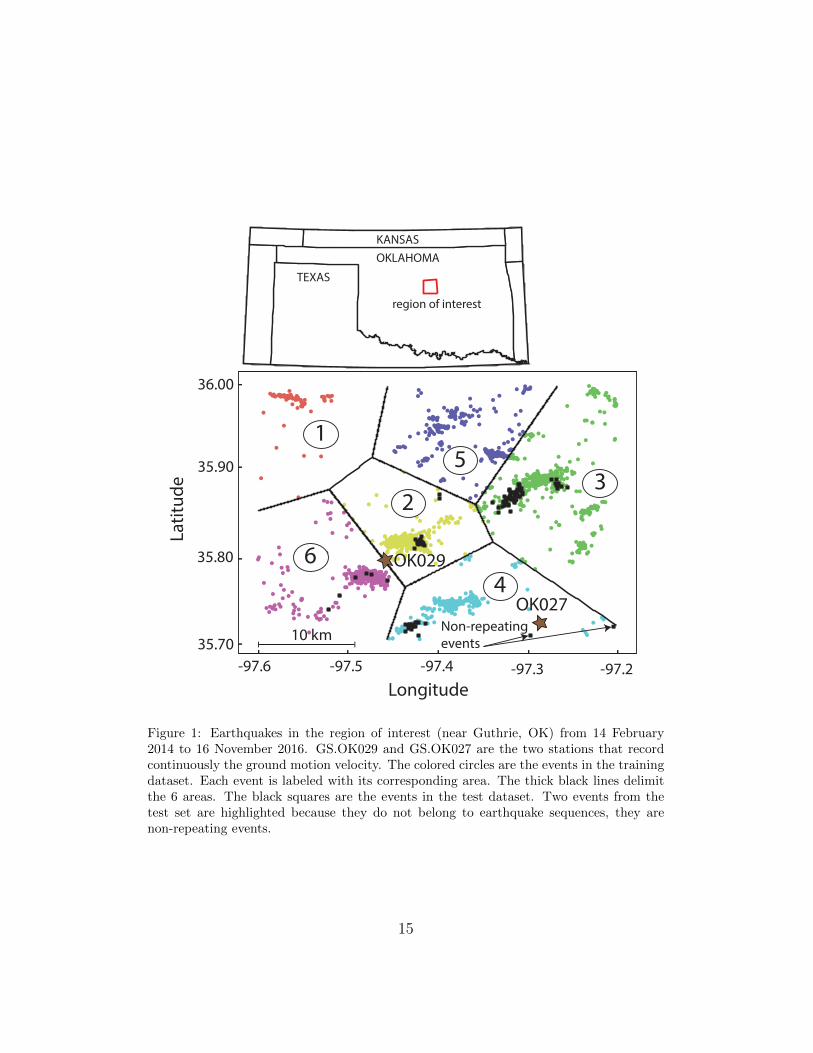
et al., 2016]. Here, we focus on the particularly active area near Guthrie54

(Oklahoma). In this region, the Oklahoma state Geological Survey (OGS)55

cataloged 2021 seismic events from 15 February 2014 to 16 November 201656

(see Figure 1). Their seismic moment magnitudes range from Mw -0.2 to Mw57

5.8. We use the continuous ground velocity records from two local stations58

GS.OK027 and GS.OK029 (see Figure 1). GS.OK027 was active from 1459

February 2014 to 3 March 2015. GS.OK029 was deployed on 15 February60

2014 and has remained active since. Signals from both stations are recorded61

at 100 Hz on 3 channels corresponding to the three spatial dimensions: HHZ62

oriented vertically, HHN oriented North-South and HHE oriented West-East.63

Generating location labels. We partition the 2021 earthquakes into 6 ge-64

ographic clusters. For this we use the K-Means algorithm [MacQueen et al.,65

1967], with the Euclidean distance between epicenters as the metric. The66

centroıds of the clusters we obtain define 6 areas on the map (Figure 1). Any67

point on the map is assigned to the cluster whose centroıd is the closest (i.e.,68

each point is assigned to its Voronoı cell). We find that 6 clusters allow for69

a reasonable partition of the major earthquake sequences. Our classification70

thus contains 7 labels, or classes in the machine learning terminology: class71

0 corresponds to seismic noise without any earthquake, classes 1 to 6 corre-72

spond to earthquakes originating from the corresponding geographic area.73

Extracting windows for classification. We divide the continuous wave-74

form data into monthly streams. We normalize each stream individually by75

subtracting the mean over the month and dividing by the absolute peak am-76

plitude (independently for each of the 3 channels). We extract two types of77

10 second long windows from these streams: windows containing events and78

windows free of events (i.e. containing only seismic noise).79

To select the event windows and attribute their geographic cluster, we use80

the catalogs from the OGS. Together, GS.OK027 and GS.OK029 yield 291881

3

windows of labeled earthquakes for the period between 15 February 2014 and82

16 November 2016.83

We look for windows of seismic noise in between the cataloged events.84

Because some of the low magnitudes earthquakes we wish to detect are most85

likely buried in seismic noise, it is important that we reduce the chance of86

mislabeling these events as noise. This is why we use a more exhaustive cat-87

alog created by Benz et al. [2015] to select our noise examples. This catalog88

covers the same geographic area but for the period between 15 February and89

31 August 2014 only and does not locate events. This yields 831,111 windows90

of seismic noise.91

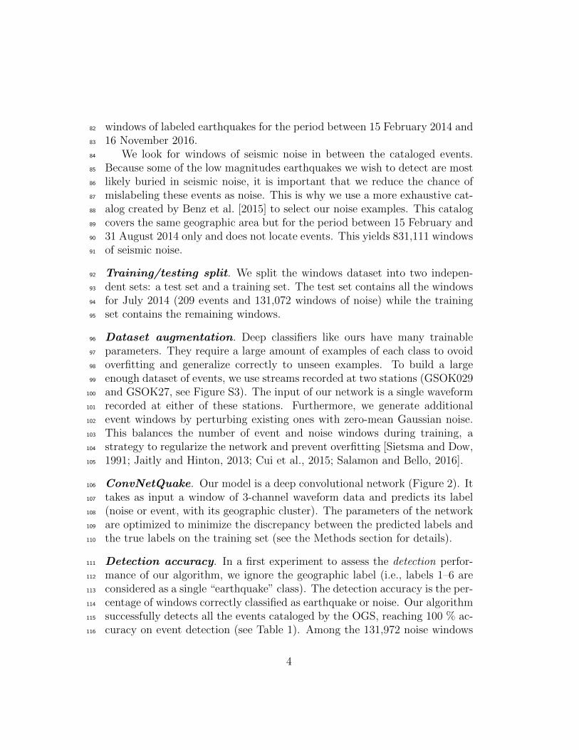
Training/testing split. We split the windows dataset into two indepen-92

dent sets: a test set and a training set. The test set contains all the windows93

for July 2014 (209 events and 131,072 windows of noise) while the training94

set contains the remaining windows.95

Dataset augmentation. Deep classifiers like ours have many trainable96

parameters. They require a large amount of examples of each class to ovoid97

overfitting and generalize correctly to unseen examples. To build a large98

enough dataset of events, we use streams recorded at two stations (GSOK02999

and GSOK27, see Figure S3). The input of our network is a single waveform100

recorded at either of these stations. Furthermore, we generate additional101

event windows by perturbing existing ones with zero-mean Gaussian noise.102

This balances the number of event and noise windows during training, a103

strategy to regularize the network and prevent overfitting [Sietsma and Dow,104

1991; Jaitly and Hinton, 2013; Cui et al., 2015; Salamon and Bello, 2016].105

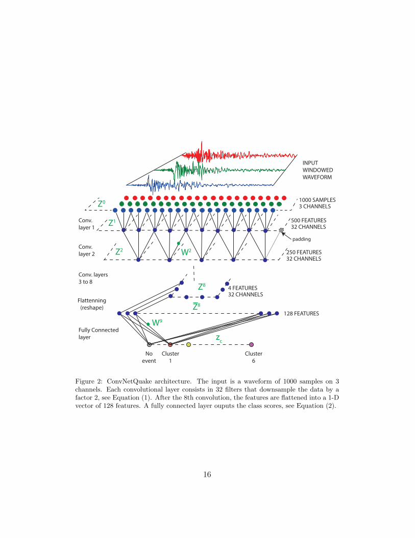
ConvNetQuake. Our model is a deep convolutional network (Figure 2). It106

takes as input a window of 3-channel waveform data and predicts its label107

(noise or event, with its geographic cluster). The parameters of the network108

are optimized to minimize the discrepancy between the predicted labels and109

the true labels on the training set (see the Methods section for details).110

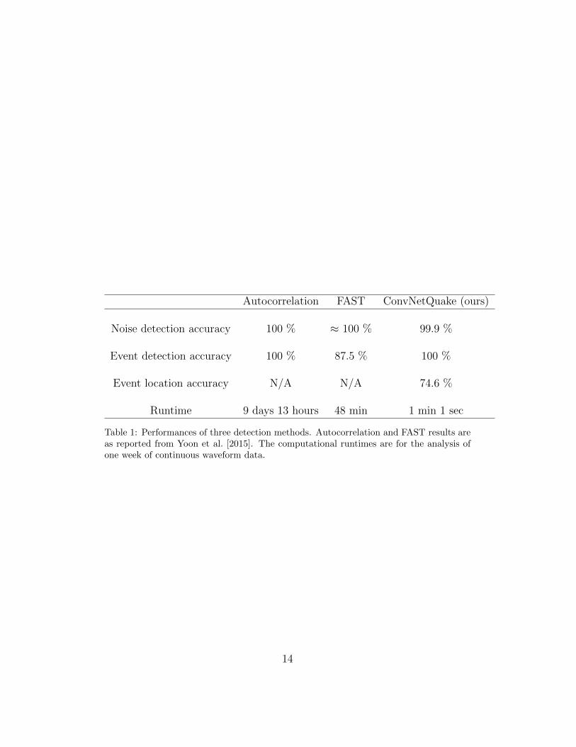
Detection accuracy. In a first experiment to assess the detection perfor-111

mance of our algorithm, we ignore the geographic label (i.e., labels 1–6 are112

considered as a single “earthquake” class). The detection accuracy is the per-113

centage of windows correctly classified as earthquake or noise. Our algorithm114

successfully detects all the events cataloged by the OGS, reaching 100 % ac-115

curacy on event detection (see Table 1). Among the 131,972 noise windows116

4

of our test set, ConvNetQuake correctly classifies 129,954 noise windows. It117

classifies 2018 of the noise windows as events. Among them, 1902 windows118

were confirmed as events by the autocorrelation method (detailed in the sup-119

plementary materials). That is, our algorithm made 116 false detections, for120

an accuracy of 99.9 % on noise windows.121

Location accuracy. We then evaluate the location performance. For each122

of the detected events, we compare the predicted class (1–6) with the true123

geographic label. We obtain 74.5 % location accuracy on the test set (see124

Table 1). For comparison with a “chance” baseline, selecting a class at125

random would give 1/6 = 16.7 % accuracy.126

We also experimented with a larger number of clusters (50, see Figure S4)127

and obtained 22.5 % in location accuracy, still 10 times better than chance at128

1/50 = 2 %. This performance drop is not surprising since, on average, each129

class now only provides 40 training samples, which is insufficient for proper130

training.131

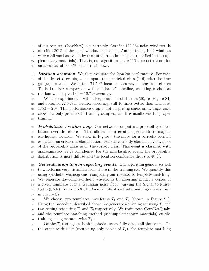
Probabilistic location map. Our network computes a probability distri-132

bution over the classes. This allows us to create a probabilistic map of133

earthquake location. We show in Figure 3 the maps for a correctly located134

event and an erroneous classification. For the correctly classified event, most135

of the probability mass is on the correct class. This event is classified with136

approximately 99 % confidence. For the misclassified event, the probability137

distribution is more diffuse and the location confidence drops to 40 %.138

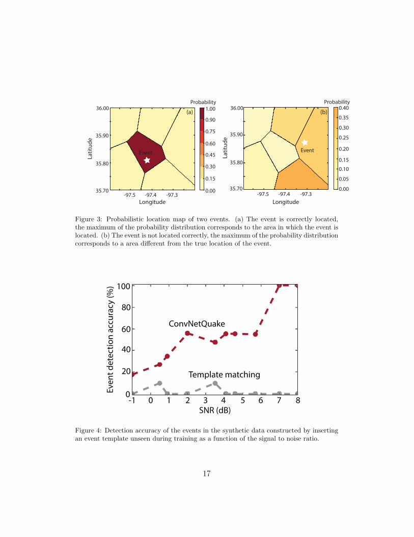
Generalization to non-repeating events. Our algorithm generalizes well139

to waveforms very dissimilar from those in the training set. We quantify this140

using synthetic seismograms, comparing our method to template matching.141

We generate day-long synthetic waveforms by inserting multiple copies of142

a given template over a Gaussian noise floor, varying the Signal-to-Noise-143

Ratio (SNR) from -1 to 8 dB. An example of synthetic seismogram is shown144

in Figure S2.145

We choose two templates waveforms T1 and T2 (shown in Figure S1).146

Using the procedure described above, we generate a training set using T1 and147

two testing sets using T1 and T2 respectively. We train both ConvNetQuake148

and the template matching method (see supplementary materials) on the149

training set (generated with T1).150

On the T1 testing set, both methods successfully detect all the events. On151

the other testing set (containing only copies of T2), the template matching152

5

method fails to detect inserted events even at high SNR. ConvNetQuake153

however recognizes the new (unknown) events. The accuracy of our model154

remarkably increases with SNR (see Figure 4). For SNRs higher than 7 dB,155

ConvNetQuake detects all the inserted seismic events.156

Many events in our dataset from Oklahoma are non-repeating events (we157

highlighted two in Figure 1). Our experiment on synthetic data suggests158

that methods relying on template matching cannot detect them while Con-159

vNetQuake can.160

Earthquake detection on continuous records. We run ConvNetQuake161

on one month of continuous waveform data recorded with GS.OK029 in July162

2014. The 3-channel waveforms are cut into 10 second long, non overlap-163

ping windows, with a 1 second offset between consecutive windows to avoid164

possibly redundant detections. Our algorithm detects 4225 events never cat-165

aloged before by the OGS. This is about 5 events per hour. Autocorrelation166

confirms 3949 of these detections (see supplementary for details). Figure 6167

shows the most repeated waveform (479 times) among the 3949 detections.168

Comparison with other detection methods. We compare our detection169

performances to autocorrelation and Fingerprint And Similarity Threshold-170

ing (FAST, reported from Yoon et al. [2015]). Both techniques can only find171

repeating events, and do not provide event location.172

Yoon et al. [2015] used autocorrelation and FAST to detect new events173

during one week of continuous waveform data recorded at a single station with174

the a single channel from 8 January 2011 to 15 January 2011. The bank of175

templates used for FAST consists in 21 earthquakes: a Mw 4.1 that occurred176

on 8 January 2011 on the Calaveras Fault (North California) and 20 of its177

aftershocks (Mw 0.84 to Mw 4.10, a range similar to our dataset). Table 1178

reports the classification accuracy of all three methods. ConvNetQuake has179

an acccuracy comparable to autocorrelation and outperforms FAST.180

Scalability to large datasets. The runtimes of the autocorrelation method,181

FAST, and ConvNetQuake necessary to analyze one week of continuous wave-182

form data are reported in Table 1. Our runtime excludes the training phase183

which is performed once. Similarly, FAST’s runtime excludes the time re-184

quired to build the database of templates. We ran our algorithm on a dual185

core Intel i5 2.9 GHz CPU. It is approximately 13,500 times faster than186

autocorrelation and 48 times faster than FAST (Table 1). ConvNetQuake187

is highly scalable and can easily handle large datasets. It can process one188

6

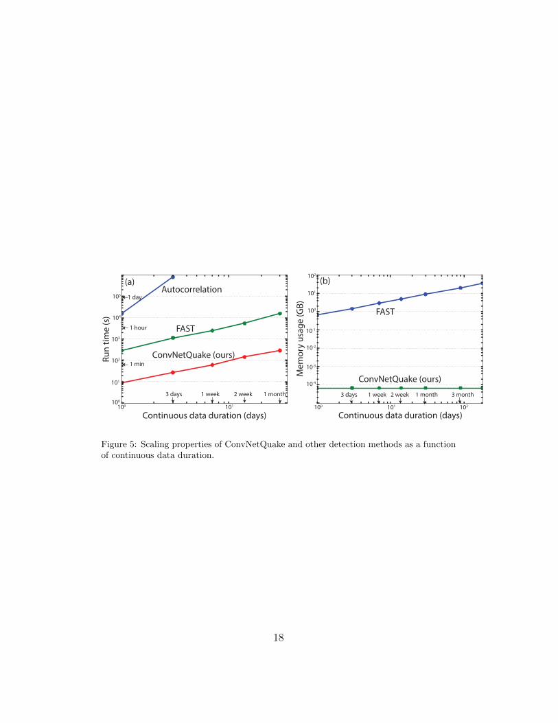
month of continuous data in 4 minutes 51 seconds while FAST is 120 times189

slower (4 hours 20 minutes, see Figure 5a).190

Like other template matching techniques, FAST’s database grows as it191

creates and store new templates during detection. For 2 days of continuous192

recording, FAST’s database is approximately 1 GB (see Figure 5b). Process-193

ing years of continuous waveform data would increase dramatically the size194

of this database and adversely affect performance. Our network only needs195

to store a compact set of parameters, which entails a constant memory usage196

(500 kB, see Figure 5b).197

Discussion198

ConvNetQuake achieves state-of-the-art performances in probabilistic event199

detection and location using a single signal. For this, it requires a pre-existing200

history of cataloged earthquakes at training time. This makes it ill-suited201

to areas of low seismicity or areas where instrumentation is recent. In this202

study we focused on local earthquakes, leaving larger scale for future work.203

Finally, we partitioned events into discrete categories that were fixed before-204

hand. One might extend our algorithm to produce continuous probabilistic205

location maps. Our approach is ideal to monitor geothermal systems, natural206

resource reservoirs, volcanoes, and seismically active and well instrumented207

plate boundaries such as the subduction zones in Japan or the San Andreas208

Fault system in California.209

Methods210

ConvNetQuake takes as input a 3-channel window of waveform data and211

predicts a discrete probability over M categories, or classes in the machine212

learning terminology. Classes 1 to M−1 correspond to predefined geographic213

“clusters” and class 0 corresponds to event-free “seismic noise”. The clusters214

for our dataset are illustrated in Figure 1. Our algorithm outputs a M -215

D vector of probabilities that the input window belongs to each of the M216

classes. Figure 2 illustrates our architecture.217

Network architecture. The network’s input is a 2-D tensor Z0c,t repre-

senting the waveform data of a fixed-length window. The rows of Z0 forc ∈ {1, 2, 3} correspond to the channels of the waveform and since we use 10second-long windows sampled at 100 Hz, the time index is t ∈ {1, . . . , 1000}.

7

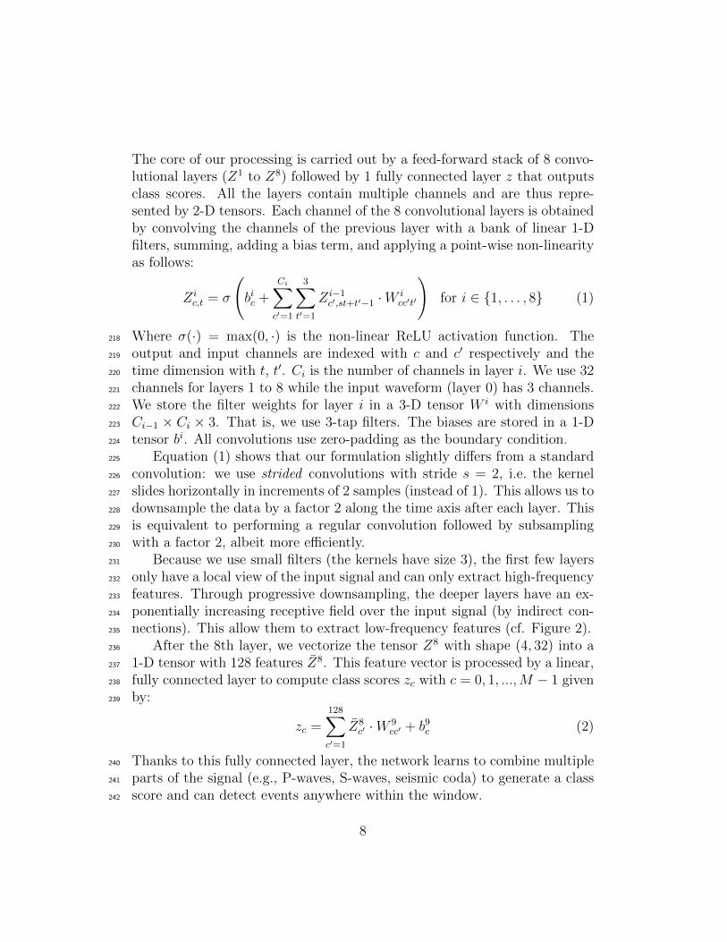
The core of our processing is carried out by a feed-forward stack of 8 convo-lutional layers (Z1 to Z8) followed by 1 fully connected layer z that outputsclass scores. All the layers contain multiple channels and are thus repre-sented by 2-D tensors. Each channel of the 8 convolutional layers is obtainedby convolving the channels of the previous layer with a bank of linear 1-Dfilters, summing, adding a bias term, and applying a point-wise non-linearityas follows:

Zic,t = σ

(bic +

Ci∑c′=1

3∑t′=1

Zi−1c′,st+t′−1 ·W

icc′t′

)for i ∈ {1, . . . , 8} (1)

Where σ(·) = max(0, ·) is the non-linear ReLU activation function. The218

output and input channels are indexed with c and c′ respectively and the219

time dimension with t, t′. Ci is the number of channels in layer i. We use 32220

channels for layers 1 to 8 while the input waveform (layer 0) has 3 channels.221

We store the filter weights for layer i in a 3-D tensor W i with dimensions222

Ci−1 × Ci × 3. That is, we use 3-tap filters. The biases are stored in a 1-D223

tensor bi. All convolutions use zero-padding as the boundary condition.224

Equation (1) shows that our formulation slightly differs from a standard225

convolution: we use strided convolutions with stride s = 2, i.e. the kernel226

slides horizontally in increments of 2 samples (instead of 1). This allows us to227

downsample the data by a factor 2 along the time axis after each layer. This228

is equivalent to performing a regular convolution followed by subsampling229

with a factor 2, albeit more efficiently.230

Because we use small filters (the kernels have size 3), the first few layers231

only have a local view of the input signal and can only extract high-frequency232

features. Through progressive downsampling, the deeper layers have an ex-233

ponentially increasing receptive field over the input signal (by indirect con-234

nections). This allow them to extract low-frequency features (cf. Figure 2).235

After the 8th layer, we vectorize the tensor Z8 with shape (4, 32) into a236

1-D tensor with 128 features Z8. This feature vector is processed by a linear,237

fully connected layer to compute class scores zc with c = 0, 1, ...,M − 1 given238

by:239

zc =128∑c′=1

Z8c′ ·W 9

cc′ + b9c (2)

Thanks to this fully connected layer, the network learns to combine multiple240

parts of the signal (e.g., P-waves, S-waves, seismic coda) to generate a class241

score and can detect events anywhere within the window.242

8

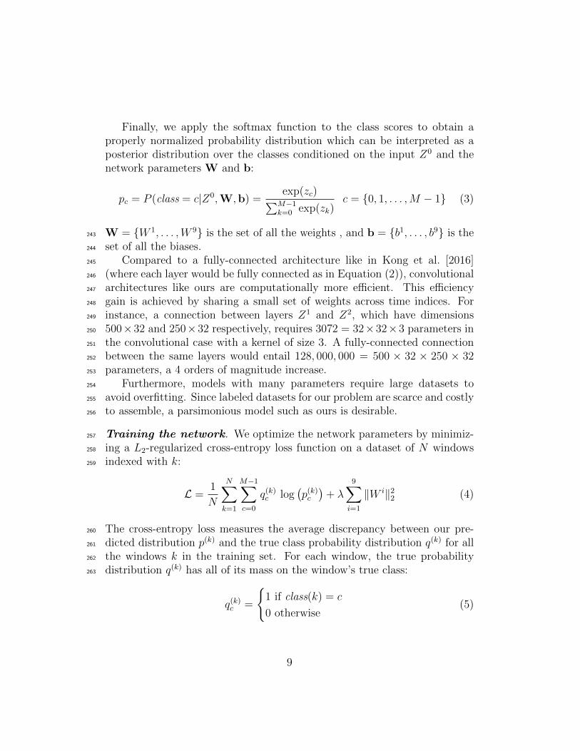
Finally, we apply the softmax function to the class scores to obtain aproperly normalized probability distribution which can be interpreted as aposterior distribution over the classes conditioned on the input Z0 and thenetwork parameters W and b:

pc = P (class = c|Z0,W,b) =exp(zc)∑M−1

k=0 exp(zk)c = {0, 1, . . . ,M − 1} (3)

W = {W 1, . . . ,W 9} is the set of all the weights , and b = {b1, . . . , b9} is the243

set of all the biases.244

Compared to a fully-connected architecture like in Kong et al. [2016]245

(where each layer would be fully connected as in Equation (2)), convolutional246

architectures like ours are computationally more efficient. This efficiency247

gain is achieved by sharing a small set of weights across time indices. For248

instance, a connection between layers Z1 and Z2, which have dimensions249

500×32 and 250×32 respectively, requires 3072 = 32×32×3 parameters in250

the convolutional case with a kernel of size 3. A fully-connected connection251

between the same layers would entail 128, 000, 000 = 500 × 32 × 250 × 32252

parameters, a 4 orders of magnitude increase.253

Furthermore, models with many parameters require large datasets to254

avoid overfitting. Since labeled datasets for our problem are scarce and costly255

to assemble, a parsimonious model such as ours is desirable.256

Training the network. We optimize the network parameters by minimiz-257

ing a L2-regularized cross-entropy loss function on a dataset of N windows258

indexed with k:259

L =1

N

N∑k=1

M−1∑c=0

q(k)c log(p(k)c

)+ λ

9∑i=1

‖W i‖22 (4)

The cross-entropy loss measures the average discrepancy between our pre-260

dicted distribution p(k) and the true class probability distribution q(k) for all261

the windows k in the training set. For each window, the true probability262

distribution q(k) has all of its mass on the window’s true class:263

q(k)c =

{1 if class(k) = c

0 otherwise(5)

9

To regularize the neural network, we add an L2 penalty on the weights264

W, balanced with the cross-entropy loss via the parameter λ = 10−3. Regu-265

larization favors network configurations with small weight magnitude. This266

reduces the potential for overfitting [Ng, 2004].267

Since both the parameter set and the training data set are too large to268

fit in memory, we minimize Equation (4) using a batched stochastic gradient269

descent algorithm. We first randomly shuffle the N = 702, 748 windows from270

the dataset. We then form a sequence of batches containing 128 windows271

each. At each training step we feed a batch to the network, evaluate the272

expected loss on the batch, and update the network parameters accordingly273

using backpropagation [LeCun et al., 2015]. We repeatedly cycle through274

the sequence until the expected loss stops improving. Since our dataset is275

unbalanced (we have many more noise windows than events), each batch is276

composed of 64 windows of noise and 64 event windows.277

For optimization we use the ADAM [Kingma and Ba, 2014] algorithm,278

which keeps track of first and second order moments of the gradients, and is279

invariant to any diagonal rescaling of the gradients. We use a learning rate280

of 10−4 and keep all other parameters to the default value recommended by281

the authors. We implemented ConvNetQuake in TensorFlow [Abadi et al.,282

2015] and performed all our trainings on a NVIDIA Tesla K20Xm Graphics283

Processing Unit. We train for 32,000 iterations which takes approximately284

1.5 h.285

Evaluation on an independent testing set. After training, we test the286

accuracy of our network on windows from July 2014 (209 windows of events287

and 131,072 windows of noise). The class predicted by our algorithm is the288

one whose posterior probability pc is the highest. We evaluate our predictions289

using two metrics. The detection accuracy is the percentage of windows290

correctly classified as events or noise. The location accuracy is the percentage291

of windows already classified as events that have the correct cluster number.292

Acknowledgments293

The ConvNetQuake software is open-source1. The waveform data used in294

this paper can be obtained from the Incorporated Research Institutions for295

Seismology (IRIS) Data Management Center and the network GS is available296

1the software can be downloaded at https://github.com/tperol/ConvNetQuake

10

at doi:10.7914/SN/GS. The earthquake catalog used is provided by the Ok-297

lahoma Geological Survey. The computations in this paper were run on the298

Odyssey cluster supported by the FAS Division of Science, Research Com-299

puting Group at Harvard University. T. P.’s research was supported by the300

National Science Foundation grant Division for Materials Research 14-20570301

to Harvard University with supplemental support by the Southern California302

Earthquake Center (SCEC), funded by NSF cooperative agreement EAR-303

1033462 and USGS cooperative agreement G12AC20038. T.P. thanks Jim304

Rice for his continuous support during his PhD and Loıc Viens for insightful305

discussions about seismology.306

References307

W. L. Ellsworth, Injection-induced earthquakes, Science 341 (2013).308

R. Allen, Automatic phase pickers: their present use and future prospects,309

Bulletin of the Seismological Society of America 72 (1982) S225–S242.310

M. Withers, R. Aster, C. Young, J. Beiriger, M. Harris, S. Moore, J. Trujillo,311

A comparison of select trigger algorithms for automated global seismic312

phase and event detection, Bulletin of the Seismological Society of America313

88 (1998) 95–106.314

S. J. Gibbons, F. Ringdal, The detection of low magnitude seismic events315

using array-based waveform correlation, Geophysical Journal International316

165 (2006) 149–166.317

R. J. Skoumal, M. R. Brudzinski, B. S. Currie, J. Levy, Optimizing318

multi-station earthquake template matching through re-examination of319

the Youngstown, Ohio, sequence, Earth and Planetary Science Letters320

405 (2014) 274–280.321

D. Harris, Subspace Detectors: Theory, Lawrence Livermore National Labo-322

ratory, Technical Report, internal report, UCRL-TR-222758, 2006.323

D. Harris, D. Dodge, An autonomous system for grouping events in a devel-324

oping aftershock sequence, Bulletin of the Seismological Society of America325

101 (2011) 763–774.326

S. A. Barrett, G. C. Beroza, An empirical approach to subspace detection,327

Seismological Research Letters 85 (2014) 594–600.328

11

H. M. Benz, N. D. McMahon, R. C. Aster, D. E. McNamara, D. B. Harris,329

Hundreds of earthquakes per day: The 2014 Guthrie, Oklahoma, earth-330

quake sequence, Seismological Research Letters 86 (2015) 1318–1325.331

C. E. Yoon, O. OReilly, K. J. Bergen, G. C. Beroza, Earthquake detection332

through computationally efficient similarity search, Science advances 1333

(2015) e1501057.334

A. Krizhevsky, I. Sutskever, G. E. Hinton, Imagenet classification with deep335

convolutional neural networks, in: Advances in neural information pro-336

cessing systems, pp. 1097–1105.337

Y. LeCun, Y. Bengio, G. Hinton, Deep learning, Nature 521 (2015) 436–444.338

A. van den Oord, S. Dieleman, H. Zen, K. Simonyan, O. Vinyals, A. Graves,339

N. Kalchbrenner, A. Senior, K. Kavukcuoglu, Wavenet: A generative340

model for raw audio, arXiv preprint arXiv:1609.03499 (2016).341

W. Xiong, J. Droppo, X. Huang, F. Seide, M. Seltzer, A. Stolcke, D. Yu,342

G. Zweig, The microsoft 2016 conversational speech recognition system,343

arXiv preprint arXiv:1609.03528 (2016).344

A. A. Holland, Earthquakes triggered by hydraulic fracturing in south-central345

Oklahoma, Bulletin of the Seismological Society of America 103 (2013)346

1784–1792.347

K. M. Keranen, H. M. Savage, G. A. Abers, E. S. Cochran, Potentially in-348

duced earthquakes in Oklahoma, USA: Links between wastewater injection349

and the 2011 Mw 5.7 earthquake sequence, Geology 41 (2013) 699–702.350

F. R. Walsh, M. D. Zoback, Oklahomas recent earthquakes and saltwater351

disposal, Science advances 1 (2015) e1500195.352

M. Weingarten, S. Ge, J. W. Godt, B. A. Bekins, J. L. Rubinstein, High-rate353

injection is associated with the increase in US mid-continent seismicity,354

Science 348 (2015) 1336–1340.355

M. Shirzaei, W. L. Ellsworth, K. F. Tiampo, P. J. Gonzalez, M. Manga,356

Surface uplift and time-dependent seismic hazard due to fluid injection in357

eastern Texas, Science 353 (2016) 1416–1419.358

12

J. MacQueen, et al., Some methods for classification and analysis of multi-359

variate observations, in: Proceedings of the fifth Berkeley symposium on360

mathematical statistics and probability, volume 1, Oakland, CA, USA.,361

pp. 281–297.362

J. Sietsma, R. J. Dow, Creating artificial neural networks that generalize,363

Neural networks 4 (1991) 67–79.364

N. Jaitly, G. E. Hinton, Vocal tract length perturbation (VTLP) improves365

speech recognition, in: Proc. ICML Workshop on Deep Learning for Audio,366

Speech and Language.367

X. Cui, V. Goel, B. Kingsbury, Data augmentation for deep neural net-368

work acoustic modeling, IEEE/ACM Transactions on Audio, Speech and369

Language Processing (TASLP) 23 (2015) 1469–1477.370

J. Salamon, J. P. Bello, Deep convolutional neural networks and data371

augmentation for environmental sound classification, arXiv preprint372

arXiv:1608.04363 (2016).373

Q. Kong, R. M. Allen, L. Schreier, Y.-W. Kwon, Myshake: A smartphone374

seismic network for earthquake early warning and beyond, Science ad-375

vances 2 (2016) e1501055.376

A. Y. Ng, Feature selection, L 1 vs. L 2 regularization, and rotational in-377

variance, in: Proceedings of the twenty-first international conference on378

Machine learning, ACM, p. 78.379

D. P. Kingma, J. Ba, Adam: A method for stochastic optimization, CoRR380

abs/1412.6980 (2014).381

M. Abadi, A. Agarwal, P. Barham, E. Brevdo, Z. Chen, C. Citro, G. S. Cor-382

rado, A. Davis, J. Dean, M. Devin, S. Ghemawat, I. Goodfellow, A. Harp,383

G. Irving, M. Isard, Y. Jia, R. Jozefowicz, L. Kaiser, M. Kudlur, J. Lev-384

enberg, D. Mane, R. Monga, S. Moore, D. Murray, C. Olah, M. Schus-385

ter, J. Shlens, B. Steiner, I. Sutskever, K. Talwar, P. Tucker, V. Van-386

houcke, V. Vasudevan, F. Viegas, O. Vinyals, P. Warden, M. Wattenberg,387

M. Wicke, Y. Yu, X. Zheng, TensorFlow: Large-scale machine learning on388

heterogeneous systems, 2015. Software available from tensorflow.org.389

13

Autocorrelation FAST ConvNetQuake (ours)

Noise detection accuracy 100 % ≈ 100 % 99.9 %

Event detection accuracy 100 % 87.5 % 100 %

Event location accuracy N/A N/A 74.6 %

Runtime 9 days 13 hours 48 min 1 min 1 sec

Table 1: Performances of three detection methods. Autocorrelation and FAST results areas reported from Yoon et al. [2015]. The computational runtimes are for the analysis ofone week of continuous waveform data.

14

1

32

4

5

6

OK027

OK029

La

titu

de

Longitude

36.00

35.90

35.80

35.70

-97.6 -97.5 -97.3-97.4 -97.2

Non-repeating

events

OKLAHOMA

TEXAS

KANSAS

region of interest

10 km

Figure 1: Earthquakes in the region of interest (near Guthrie, OK) from 14 February2014 to 16 November 2016. GS.OK029 and GS.OK027 are the two stations that recordcontinuously the ground motion velocity. The colored circles are the events in the trainingdataset. Each event is labeled with its corresponding area. The thick black lines delimitthe 6 areas. The black squares are the events in the test dataset. Two events from thetest set are highlighted because they do not belong to earthquake sequences, they arenon-repeating events.

15

Flattenning

(reshape)

No

event

Cluster

1

Cluster

6

INPUT

WINDOWED

WAVEFORM

3 CHANNELS1000 SAMPLES

32 CHANNELS500 FEATURES

32 CHANNELS250 FEATURES

32 CHANNELS4 FEATURES

W2

Conv.

layer 1

Conv.

layer 2

Conv. layers

3 to 8

128 FEATURES

W9

Fully Connected

layer

Z1

Z2

Z8

zc

padding

Z8

Z0

Figure 2: ConvNetQuake architecture. The input is a waveform of 1000 samples on 3channels. Each convolutional layer consists in 32 filters that downsample the data by afactor 2, see Equation (1). After the 8th convolution, the features are flattened into a 1-Dvector of 128 features. A fully connected layer ouputs the class scores, see Equation (2).

16

36.00

35.90

35.80

35.70-97.5 -97.3-97.4

Event

Latitude

Longitude

Event

36.00

35.90

35.80

35.70-97.5 -97.3-97.4

Longitude

Latitude

Probability

0.00

0.15

0.30

0.45

0.60

0.75

0.90

1.00

0.00

0.05

0.10

0.15

0.20

0.25

0.30

0.35

0.40Probability

(a) (b)

Figure 3: Probabilistic location map of two events. (a) The event is correctly located,the maximum of the probability distribution corresponds to the area in which the event islocated. (b) The event is not located correctly, the maximum of the probability distributioncorresponds to a area different from the true location of the event.

SNR (dB)0-1 21 43 65 87

100

80

60

40

20

0Ev

en

t d

ete

ctio

n a

ccu

rac

y (

%)

ConvNetQuake

Template matching

Figure 4: Detection accuracy of the events in the synthetic data constructed by insertingan event template unseen during training as a function of the signal to noise ratio.

17

Continuous data duration (days)

3 days 1 week 2 week 1 month

Ru

n t

ime

(s)

FAST

Autocorrelation

ConvNetQuake (ours)1 min

1 hour

1 day

101100100

105

104

103

102

101

3 days 1 week 2 week 1 month 3 month

ConvNetQuake (ours)

FAST

Me

mo

ry u

sag

e (

GB

)

Continuous data duration (days)100 101 102

102

101

100

10-1

10-2

10-3

10-4

(a) (b)

Figure 5: Scaling properties of ConvNetQuake and other detection methods as a functionof continuous data duration.

18

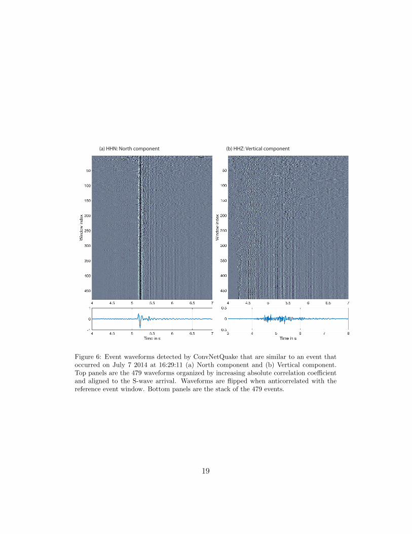
(a) HHN: North component (b) HHZ: Vertical component

Figure 6: Event waveforms detected by ConvNetQuake that are similar to an event thatoccurred on July 7 2014 at 16:29:11 (a) North component and (b) Vertical component.Top panels are the 479 waveforms organized by increasing absolute correlation coefficientand aligned to the S-wave arrival. Waveforms are flipped when anticorrelated with thereference event window. Bottom panels are the stack of the 479 events.

19