11/19/2018

1

Convolutional Neural Networks

Presented by: Ke Yu

11/13/2018

Outline

• Neural networks recap

• Building blocks of CNN

• Architectures of CNN

• Visualizing and understanding CNN

• More applications

11/19/2018

2

Neural Networks Recap

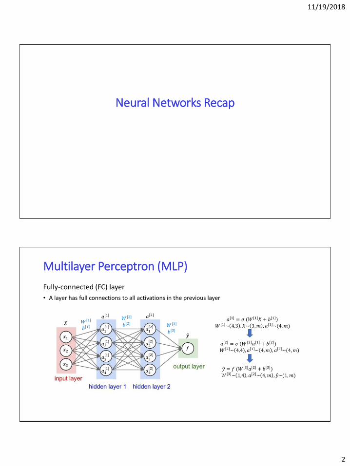
Multilayer Perceptron (MLP)

Fully-connected (FC) layer

• A layer has full connections to all activations in the previous layer

𝑋

𝑥1

𝑥2

𝑥3

𝑎[1] 𝑎[2]

𝑎1[1]

𝑎2[1]

𝑎3[1]

𝑎4[1]

𝑎1[2]

𝑎2[2]

𝑎3[2]

𝑎4[2]

ො𝑦

𝑊 [1]

𝑏[1]

𝑊 [2]

𝑏[2] 𝑊 [3]

𝑏[3]

𝑓

𝑎[1] = 𝜎 (𝑊[1]𝑋 + 𝑏[1])

𝑊 [1]~ 4,3 , 𝑋~ 3,𝑚 , 𝑎[1]~(4,𝑚)

𝑎[2] = 𝜎 (𝑊[2]𝑎[1] + 𝑏[2])

𝑊 [2]~ 4,4 , 𝑎[1]~ 4,𝑚 , 𝑎[2]~(4,𝑚)

ො𝑦 = 𝑓 (𝑊[3]𝑎[2] + 𝑏[3])

𝑊 [3]~ 1,4 , 𝑎[2]~ 4,𝑚 , ො𝑦~(1,𝑚)

11/19/2018

3

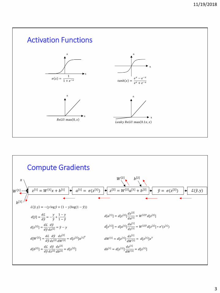
Activation Functions

a

x

x

a

x

a

x

a

𝜎 𝑥 =1

1 + 𝑒−𝑥 𝑡𝑎𝑛ℎ 𝑥 =𝑒𝑥 − 𝑒−𝑥

𝑒𝑥 + 𝑒−𝑥

𝑅𝑒𝐿𝑈:max 0, 𝑥𝐿𝑒𝑎𝑘𝑦 𝑅𝑒𝐿𝑈:max 0.1𝑥, 𝑥

Compute Gradients

𝑧[1] = 𝑊[1]𝑥 + 𝑏[1]

𝑥

𝑊[1]

𝑏[1]

𝑎[1] = 𝜎(𝑧[1]) ℒ( ො𝑦, y)𝑧[2] = 𝑊[2]𝑎[1] + 𝑏[2] ො𝑦 = 𝜎(𝑧[2])

𝑊[2] 𝑏[2]

ℒ ො𝑦, y = −(𝑦 log ො𝑦 + 1 − 𝑦 log(1 − ො𝑦))

𝑑[ ො𝑦] =𝑑ℒ

𝑑 ො𝑦= −

𝑦

ො𝑦+1 − 𝑦

1 − ො𝑦

𝑑[𝑧 2 ] =𝑑ℒ

𝑑 ො𝑦

𝑑 ො𝑦

𝑑𝑧[2]= ො𝑦 − 𝑦

𝑑[𝑊 2 ] =𝑑ℒ

𝑑 ො𝑦

𝑑 ො𝑦

𝑑𝑧 2

𝑑𝑧 2

𝑑𝑊 2= 𝑑[𝑧 2 ]𝑎 1 𝑇

𝑑[𝑏[2]] =𝑑ℒ

𝑑 ො𝑦

𝑑 ො𝑦

𝑑𝑧[2]𝑑𝑧[2]

𝑑𝑏 2= 𝑑[𝑧 2 ]

𝑑 𝑧 1 = 𝑑[𝑎[1]]𝑑𝑎[1]

𝑑𝑧 1= 𝑊 2 𝑇𝑑[𝑧 2 ] ∗ 𝜎′(z 1 )

𝑑[𝑎[1]] = 𝑑[𝑧 2 ]𝑑𝑧 2

𝑑𝑎 1= 𝑊 2 𝑇𝑑[𝑧 2 ]

𝑑𝑊 [1] = 𝑑[𝑧[1]]𝑑𝑧[1]

𝑑𝑊 1= 𝑑[𝑧[1]]𝑥𝑇

𝑑𝑏[1] = 𝑑[𝑧[1]]𝑑𝑧[1]

𝑑𝑊 1= 𝑑[𝑧[1]]

11/19/2018

4

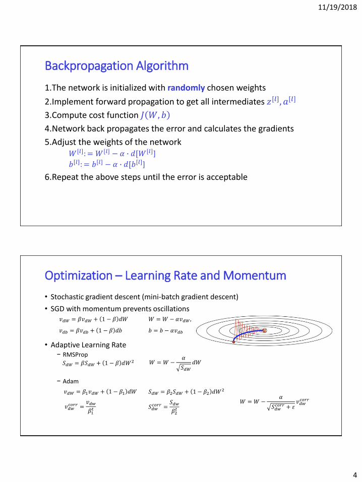
Backpropagation Algorithm

1.The network is initialized with randomly chosen weights

2.Implement forward propagation to get all intermediates 𝑧[𝑙], 𝑎[𝑙]

3.Compute cost function 𝐽 𝑊, 𝑏

4.Network back propagates the error and calculates the gradients

5.Adjust the weights of the network 𝑊[𝑙]: = 𝑊[𝑙] − 𝛼 ∙ 𝑑[𝑊[𝑙]]

𝑏[𝑙]: = 𝑏[𝑙] − 𝛼 ∙ 𝑑[𝑏[𝑙]]

6.Repeat the above steps until the error is acceptable

Optimization – Learning Rate and Momentum

• Stochastic gradient descent (mini-batch gradient descent)

• SGD with momentum prevents oscillations

• Adaptive Learning Rate− RMSProp

− Adam

𝑣𝑑𝑊 = 𝛽𝑣𝑑𝑊 + 1 − 𝛽 𝑑𝑊

𝑣𝑑𝑏 = 𝛽𝑣𝑑𝑏 + 1 − 𝛽 𝑑𝑏

𝑊 = 𝑊 − 𝛼𝑣𝑑𝑊,

𝑏 = 𝑏 − 𝛼𝑣𝑑𝑏

𝑆𝑑𝑊 = 𝛽𝑆𝑑𝑊 + 1 − 𝛽 𝑑𝑊2 𝑊 = 𝑊 −𝛼

𝑆𝑑𝑊𝑑𝑊

𝑣𝑑𝑊 = 𝛽1𝑣𝑑𝑊 + 1 − 𝛽1 𝑑𝑊 𝑆𝑑𝑊 = 𝛽2𝑆𝑑𝑊 + 1 − 𝛽2 𝑑𝑊2

𝑣𝑑𝑤𝑐𝑜𝑟𝑟 =

𝑣𝑑𝑤

𝛽1𝑡 𝑆𝑑𝑤

𝑐𝑜𝑟𝑟 =𝑆𝑑𝑤

𝛽2𝑡

𝑊 = 𝑊 −𝛼

𝑆𝑑𝑤𝑐𝑜𝑟𝑟 + 𝜀

𝑣𝑑𝑤𝑐𝑜𝑟𝑟

11/19/2018

5

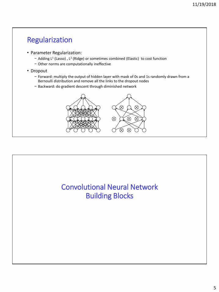
Regularization

• Parameter Regularization:− Adding L1 (Lasso) , L2 (Ridge) or sometimes combined (Elastic) to cost function

− Other norms are computationally ineffective

• Dropout− Forward: multiply the output of hidden layer with mask of 0s and 1s randomly drawn from a

Bernoulli distribution and remove all the links to the dropout nodes

− Backward: do gradient descent through diminished network

Convolutional Neural NetworkBuilding Blocks

11/19/2018

6

Why not just use a MLP for images?

• MLP connects each pixel in an image to each neuron and suffers from the curse of dimensionality, so it does not scale well to higher resolution images.

• For example: a small 200 × 200 pixel RGB image the first weight matrix of FC would have 200 × 200 × 3 × #𝑛𝑒𝑢𝑟𝑜𝑛 = 12,000 ×#𝑛𝑒𝑢𝑟𝑜𝑛 parameters for the first layer alone

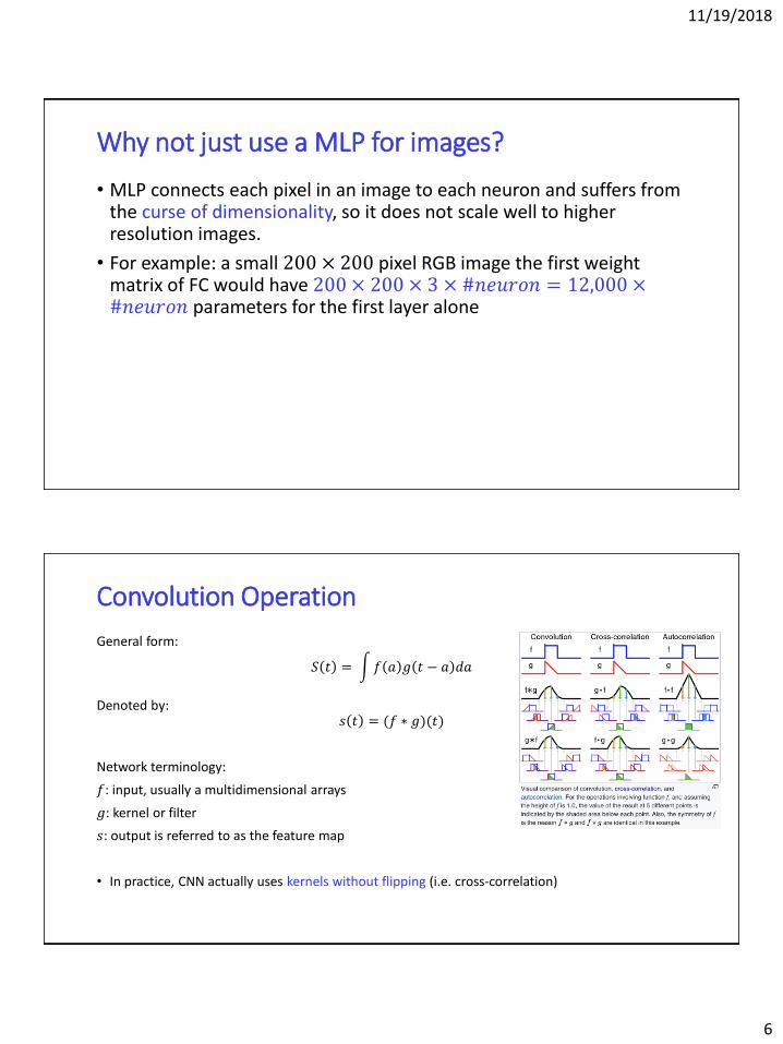
Convolution Operation

General form:

𝑆 𝑡 = න𝑓 𝑎 𝑔 𝑡 − 𝑎 𝑑𝑎

Denoted by:𝑠 𝑡 = (𝑓 ∗ 𝑔)(𝑡)

Network terminology:

𝑓: input, usually a multidimensional arrays

𝑔: kernel or filter

𝑠: output is referred to as the feature map

• In practice, CNN actually uses kernels without flipping (i.e. cross-correlation)

11/19/2018

7

Fast Fourier Transforms on GPUs

• Convolution theorem: Fourier transfer of a convolution of two signals is the pointwise product of their Fourier transforms.

• Fast Fourier transfer (FFT) reduces the complexity of convolution from 𝑂(𝑛2) to 𝑂(𝑛log 𝑛 )

• GPU-accelerated FFT implementations that perform up to 10 times faster than CPU only alternatives. (e.g. NVIDIA CUDA libraries)

ℱ 𝑥 ∗ 𝑤 = ℱ 𝑥 ∙ ℱ 𝑤

𝑥 ∗ 𝑤 = ℱ−1{ℱ 𝑥 ∙ ℱ 𝑤 }

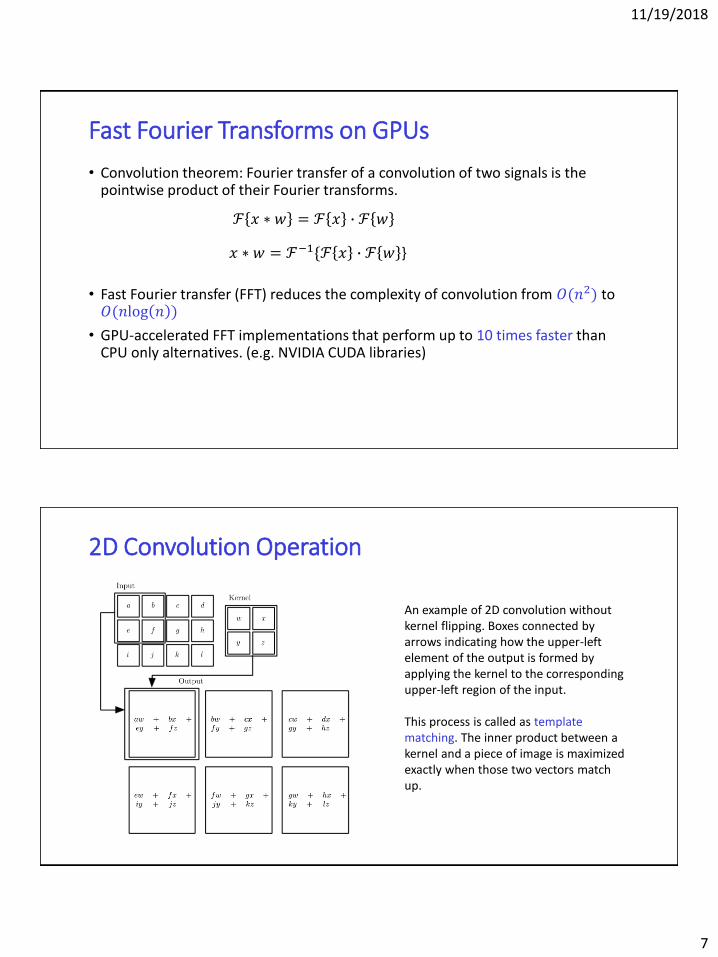
2D Convolution Operation

An example of 2D convolution without kernel flipping. Boxes connected by arrows indicating how the upper-left element of the output is formed by applying the kernel to the corresponding upper-left region of the input.

This process is called as template matching. The inner product between a kernel and a piece of image is maximized exactly when those two vectors match up.

11/19/2018

8

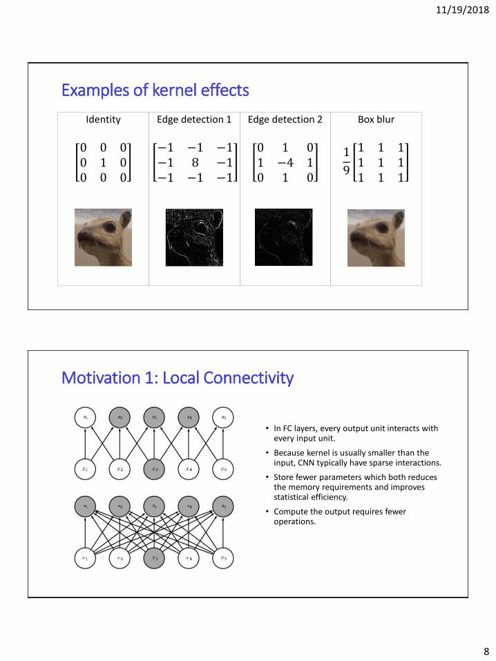
Examples of kernel effects

Identity

0 0 00 1 00 0 0

Edge detection 1

−1 −1 −1−1 8 −1−1 −1 −1

Edge detection 2

0 1 01 −4 10 1 0

Box blur

1

9

1 1 11 1 11 1 1

Motivation 1: Local Connectivity

• In FC layers, every output unit interacts with every input unit.

• Because kernel is usually smaller than the input, CNN typically have sparse interactions.

• Store fewer parameters which both reduces the memory requirements and improves statistical efficiency.

• Compute the output requires fewer operations.

11/19/2018

9

Motivation 1: Local Connectivity

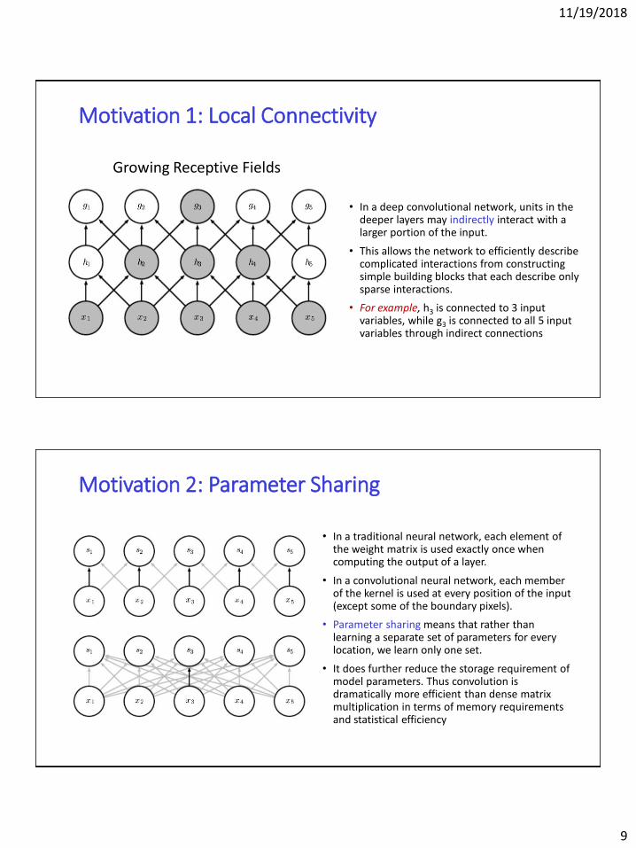
• In a deep convolutional network, units in the deeper layers may indirectly interact with a larger portion of the input.

• This allows the network to efficiently describe complicated interactions from constructing simple building blocks that each describe only sparse interactions.

• For example, h3 is connected to 3 input variables, while g3 is connected to all 5 input variables through indirect connections

Growing Receptive Fields

Motivation 2: Parameter Sharing

• In a traditional neural network, each element of the weight matrix is used exactly once when computing the output of a layer.

• In a convolutional neural network, each member of the kernel is used at every position of the input (except some of the boundary pixels).

• Parameter sharing means that rather than learning a separate set of parameters for every location, we learn only one set.

• It does further reduce the storage requirement of model parameters. Thus convolution is dramatically more efficient than dense matrix multiplication in terms of memory requirements and statistical efficiency

11/19/2018

10

Motivation 2: Parameter Sharing

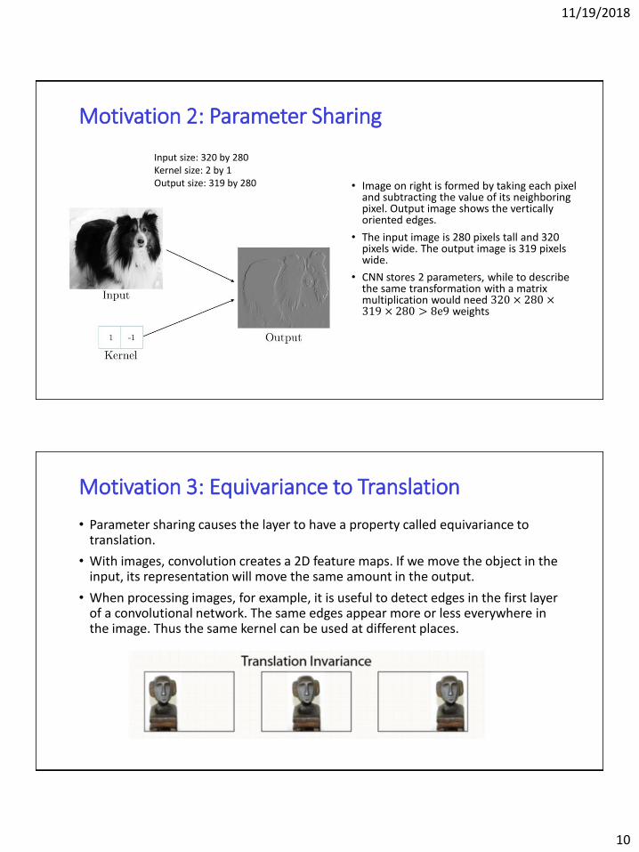
• Image on right is formed by taking each pixel and subtracting the value of its neighboring pixel. Output image shows the vertically oriented edges.

• The input image is 280 pixels tall and 320 pixels wide. The output image is 319 pixels wide.

• CNN stores 2 parameters, while to describe the same transformation with a matrix multiplication would need 320 × 280 ×319 × 280 > 8e9 weights

Input size: 320 by 280Kernel size: 2 by 1Output size: 319 by 280

Motivation 3: Equivariance to Translation

• Parameter sharing causes the layer to have a property called equivariance to translation.

• With images, convolution creates a 2D feature maps. If we move the object in the input, its representation will move the same amount in the output.

• When processing images, for example, it is useful to detect edges in the first layer of a convolutional network. The same edges appear more or less everywhere in the image. Thus the same kernel can be used at different places.

11/19/2018

11

Padding

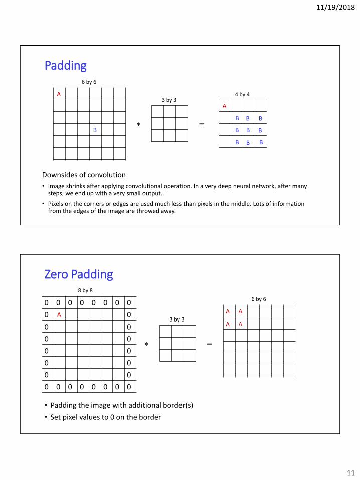
Downsides of convolution

• Image shrinks after applying convolutional operation. In a very deep neural network, after many steps, we end up with a very small output.

• Pixels on the corners or edges are used much less than pixels in the middle. Lots of information from the edges of the image are throwed away.

∗ =

6 by 6

3 by 34 by 4A

B

A

BBB

B B B

B B B

Zero Padding

• Padding the image with additional border(s)

• Set pixel values to 0 on the border

0 0 0 0 0 0 0 0

0 0

0 0

0 0

0 0

0 0

0 0

0 0 0 0 0 0 0 0

∗ =

3 by 3

6 by 6

8 by 8

A A

A

A

A

11/19/2018

12

Zero Padding Graph

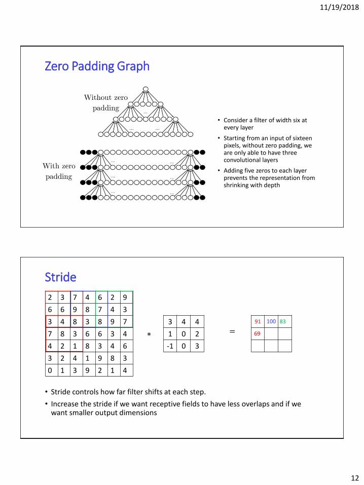
• Consider a filter of width six at every layer

• Starting from an input of sixteen pixels, without zero padding, we are only able to have three convolutional layers

• Adding five zeros to each layer prevents the representation from shrinking with depth

Stride

• Stride controls how far filter shifts at each step.

• Increase the stride if we want receptive fields to have less overlaps and if we want smaller output dimensions

2 3 7 4 6 2 9

6 6 9 8 7 4 3

3 4 8 3 8 9 7

7 8 3 6 6 3 4

4 2 1 8 3 4 6

3 2 4 1 9 8 3

0 1 3 9 2 1 4

∗

3 4 4

1 0 2

-1 0 3

=

91 100 83

69

11/19/2018

13

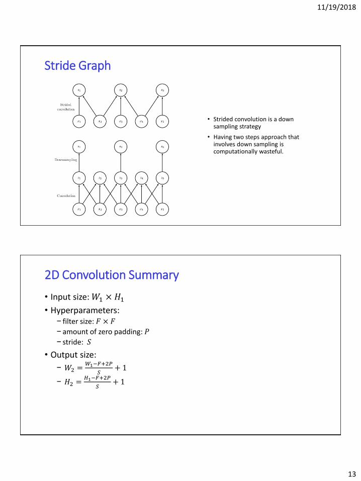
Stride Graph

• Strided convolution is a down sampling strategy

• Having two steps approach that involves down sampling is computationally wasteful.

2D Convolution Summary

• Input size: 𝑊1 × 𝐻1• Hyperparameters:

− filter size: 𝐹 × 𝐹

− amount of zero padding: 𝑃

− stride: 𝑆

• Output size:

− 𝑊2 =𝑊1−𝐹+2𝑃

𝑆+ 1

− 𝐻2 =𝐻1−𝐹+2𝑃

𝑆+ 1

11/19/2018

14

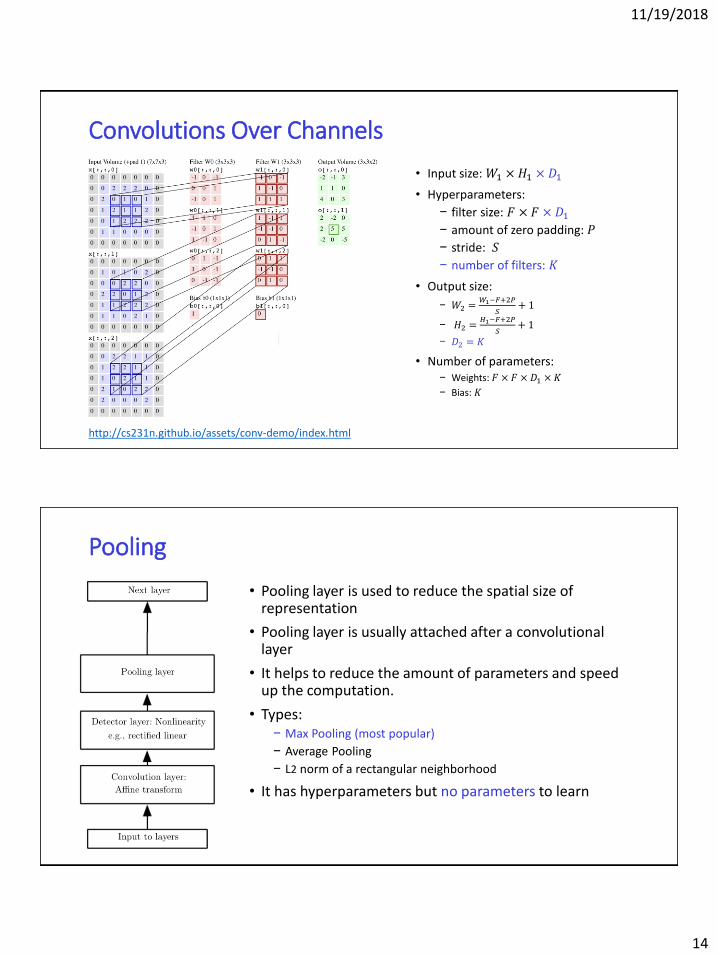
Convolutions Over Channels

• Input size: 𝑊1 × 𝐻1 × 𝐷1

• Hyperparameters:

− filter size: 𝐹 × 𝐹 × 𝐷1− amount of zero padding: 𝑃

− stride: 𝑆

− number of filters: 𝐾

• Output size:

− 𝑊2 =𝑊1−𝐹+2𝑃

𝑆+ 1

− 𝐻2 =𝐻1−𝐹+2𝑃

𝑆+ 1

− 𝐷2 = 𝐾

• Number of parameters:− Weights: 𝐹 × 𝐹 × 𝐷1 ×𝐾

− Bias: 𝐾

http://cs231n.github.io/assets/conv-demo/index.html

Pooling

• Pooling layer is used to reduce the spatial size of representation

• Pooling layer is usually attached after a convolutional layer

• It helps to reduce the amount of parameters and speed up the computation.

• Types:− Max Pooling (most popular)

− Average Pooling

− L2 norm of a rectangular neighborhood

• It has hyperparameters but no parameters to learn

11/19/2018

15

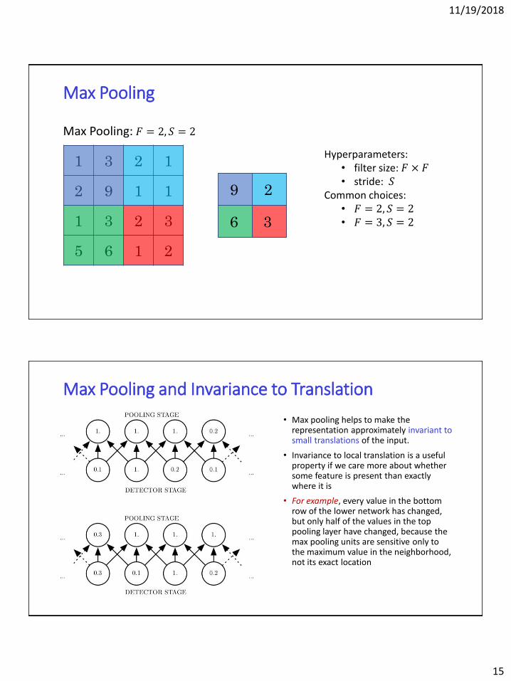
Max Pooling

1 3 2 1

2 9 1 1

1 3 2 3

5 6 1 2

Max Pooling: 𝐹 = 2, 𝑆 = 2

9 2

6 3

Hyperparameters:• filter size: 𝐹 × 𝐹• stride: 𝑆

Common choices:• 𝐹 = 2, 𝑆 = 2• 𝐹 = 3, 𝑆 = 2

Max Pooling and Invariance to Translation

• Max pooling helps to make the representation approximately invariant to small translations of the input.

• Invariance to local translation is a useful property if we care more about whether some feature is present than exactly where it is

• For example, every value in the bottom row of the lower network has changed, but only half of the values in the top pooling layer have changed, because the max pooling units are sensitive only to the maximum value in the neighborhood, not its exact location

11/19/2018

16

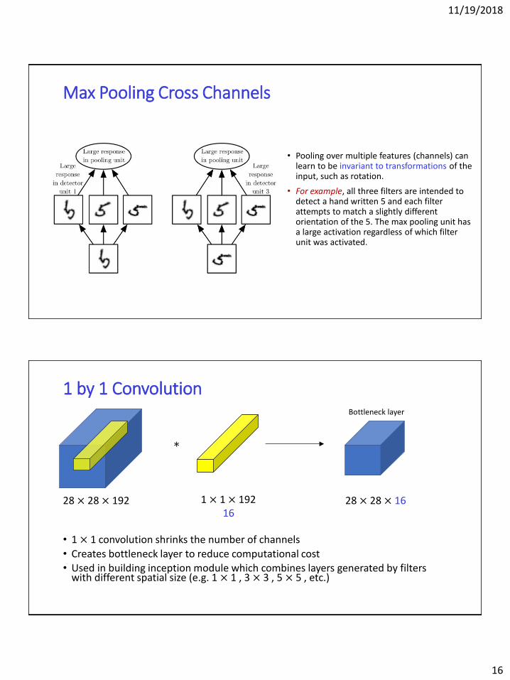
Max Pooling Cross Channels

• Pooling over multiple features (channels) can learn to be invariant to transformations of the input, such as rotation.

• For example, all three filters are intended to detect a hand written 5 and each filter attempts to match a slightly different orientation of the 5. The max pooling unit has a large activation regardless of which filter unit was activated.

1 by 1 Convolution

• 1 × 1 convolution shrinks the number of channels

• Creates bottleneck layer to reduce computational cost• Used in building inception module which combines layers generated by filters

with different spatial size (e.g. 1 × 1 , 3 × 3 , 5 × 5 , etc.)

∗

28 × 28 × 192 1 × 1 × 19216

28 × 28 × 16

Bottleneck layer

11/19/2018

17

Convolutional Neural NetworkArchitectures

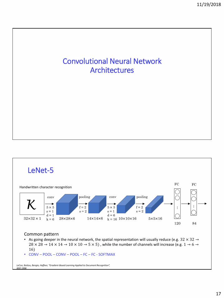
LeNet-5

⋮ ⋮

32×32 × 1 28×28×6 14×14×6 10×10×16 5×5×16

120 84

5 × 5

s = 1

d = 1

k = 6

f = 2

s = 2

pooling

5 × 5

s = 1

d = 6

k = 16

pooling

f = 2

s = 2K

Handwritten character recognition

conv conv

FC FC

Common pattern• As going deeper in the neural network, the spatial representation will usually reduce (e.g. 32 × 32 →28 × 28 → 14 × 14 → 10 × 10 → 5 × 5) , while the number of channels will increase (e.g. 1 → 6 →16)

• CONV – POOL – CONV – POOL – FC – FC - SOFTMAX

LeCun, Bottou, Bengio, Haffner, “Gradient-Based Learning Applied to Document Recognition”, IEEE 1998

11/19/2018

18

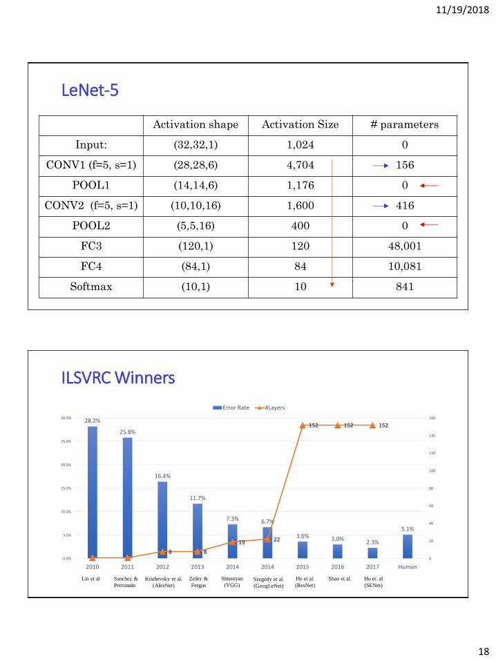
LeNet-5

Activation shape Activation Size # parameters

Input: (32,32,1) 1,024 0

CONV1 (f=5, s=1) (28,28,6) 4,704 156

POOL1 (14,14,6) 1,176 0

CONV2 (f=5, s=1) (10,10,16) 1,600 416

POOL2 (5,5,16) 400 0

FC3 (120,1) 120 48,001

FC4 (84,1) 84 10,081

Softmax (10,1) 10 841

ILSVRC Winners

28.2%

25.8%

16.4%

11.7%

7.3% 6.7%

3.6% 3.0%2.3%

5.1%

8 8

19 22

152 152 152

0

20

40

60

80

100

120

140

160

0.0%

5.0%

10.0%

15.0%

20.0%

25.0%

30.0%

2010 2011 2012 2013 2014 2014 2015 2016 2017 Human

Error Rate #Layers

Lin et al Sanchez &

Perronnin

Krizhevsky et al.

(AlexNet)

Zeiler &

Fergus

Simonyan

(VGG)Szegedy et al.

(GoogLeNet)

He et al.

(ResNet)

Shao et al. Hu et. al

(SENet)

11/19/2018

19

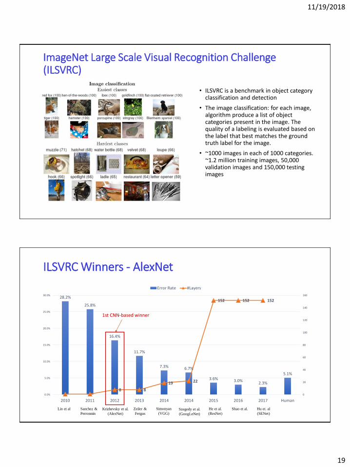
ImageNet Large Scale Visual Recognition Challenge (ILSVRC)

• ILSVRC is a benchmark in object category classification and detection

• The image classification: for each image, algorithm produce a list of object categories present in the image. The quality of a labeling is evaluated based on the label that best matches the ground truth label for the image.

• ~1000 images in each of 1000 categories. ~1.2 million training images, 50,000 validation images and 150,000 testing images

ILSVRC Winners - AlexNet

28.2%

25.8%

16.4%

11.7%

7.3% 6.7%

3.6% 3.0%2.3%

5.1%

8 8

19 22

152 152 152

0

20

40

60

80

100

120

140

160

0.0%

5.0%

10.0%

15.0%

20.0%

25.0%

30.0%

2010 2011 2012 2013 2014 2014 2015 2016 2017 Human

Error Rate #Layers

Lin et al Sanchez &

Perronnin

Krizhevsky et al.

(AlexNet)

Zeiler &

Fergus

Simonyan

(VGG)Szegedy et al.

(GoogLeNet)

He et al.

(ResNet)

Shao et al. Hu et. al

(SENet)

1st CNN-based winner

11/19/2018

20

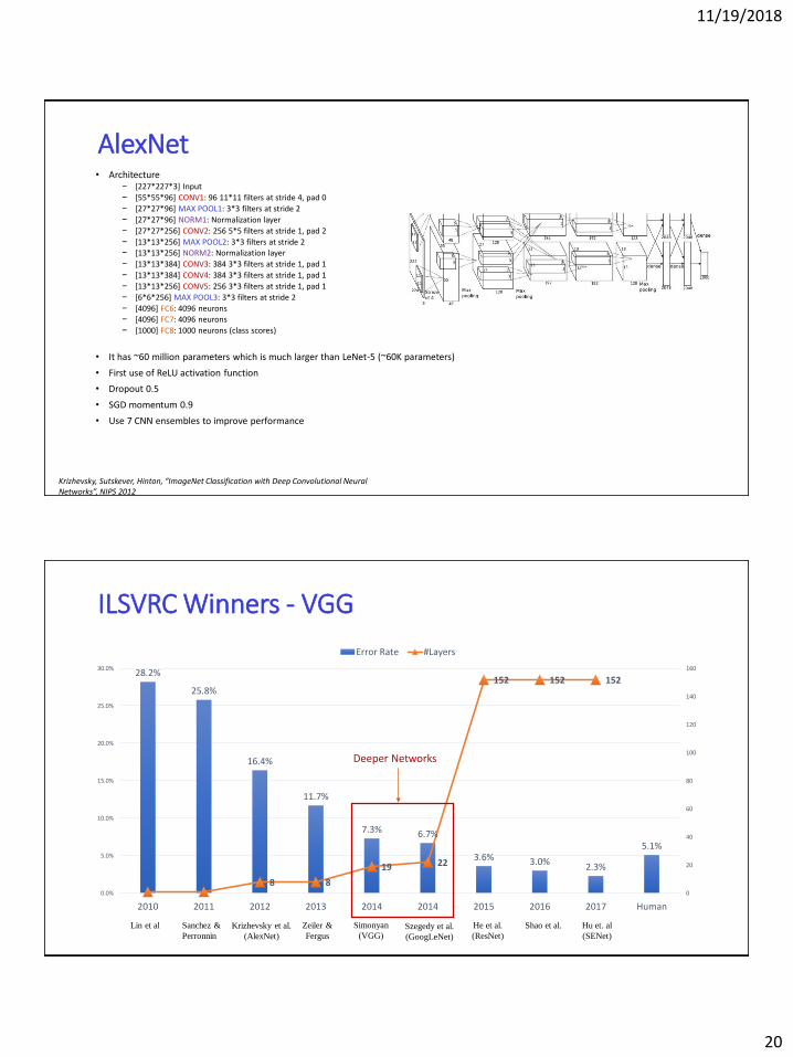
AlexNet• Architecture

− [227*227*3] Input

− [55*55*96] CONV1: 96 11*11 filters at stride 4, pad 0

− [27*27*96] MAX POOL1: 3*3 filters at stride 2

− [27*27*96] NORM1: Normalization layer

− [27*27*256] CONV2: 256 5*5 filters at stride 1, pad 2

− [13*13*256] MAX POOL2: 3*3 filters at stride 2− [13*13*256] NORM2: Normalization layer

− [13*13*384] CONV3: 384 3*3 filters at stride 1, pad 1

− [13*13*384] CONV4: 384 3*3 filters at stride 1, pad 1

− [13*13*256] CONV5: 256 3*3 filters at stride 1, pad 1

− [6*6*256] MAX POOL3: 3*3 filters at stride 2

− [4096] FC6: 4096 neurons− [4096] FC7: 4096 neurons

− [1000] FC8: 1000 neurons (class scores)

• It has ~60 million parameters which is much larger than LeNet-5 (~60K parameters)

• First use of ReLU activation function

• Dropout 0.5

• SGD momentum 0.9

• Use 7 CNN ensembles to improve performance

Krizhevsky, Sutskever, Hinton, “ImageNet Classification with Deep Convolutional Neural Networks”, NIPS 2012

ILSVRC Winners - VGG

28.2%

25.8%

16.4%

11.7%

7.3% 6.7%

3.6% 3.0%2.3%

5.1%

8 8

19 22

152 152 152

0

20

40

60

80

100

120

140

160

0.0%

5.0%

10.0%

15.0%

20.0%

25.0%

30.0%

2010 2011 2012 2013 2014 2014 2015 2016 2017 Human

Error Rate #Layers

Lin et al Sanchez &

Perronnin

Krizhevsky et al.

(AlexNet)

Zeiler &

Fergus

Simonyan

(VGG)Szegedy et al.

(GoogLeNet)

He et al.

(ResNet)

Shao et al. Hu et. al

(SENet)

Deeper Networks

11/19/2018

21

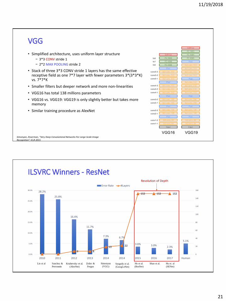
VGG

• Simplified architecture, uses uniform layer structure

− 3*3 CONV stride 1

− 2*2 MAX POOLING stride 2

• Stack of three 3*3 CONV stride 1 layers has the same effective receptive field as one 7*7 layer with fewer parameters 3*(3*3*K) vs. 7*7*K

• Smaller filters but deeper network and more non-linearities

• VGG16 has total 138 millions parameters

• VGG16 vs. VGG19: VGG19 is only slightly better but takes more memory

• Similar training procedure as AlexNet

Simonyan, Zisserman, “Very Deep Convolutional Networks For Large-Scale Image Recognition”, ICLR 2015

ILSVRC Winners - ResNet

28.2%

25.8%

16.4%

11.7%

7.3% 6.7%

3.6% 3.0%2.3%

5.1%

8 8

19 22

152 152 152

0

20

40

60

80

100

120

140

160

0.0%

5.0%

10.0%

15.0%

20.0%

25.0%

30.0%

2010 2011 2012 2013 2014 2014 2015 2016 2017 Human

Error Rate #Layers

Lin et al Sanchez &

Perronnin

Krizhevsky et al.

(AlexNet)

Zeiler &

Fergus

Simonyan

(VGG)Szegedy et al.

(GoogLeNet)

He et al.

(ResNet)

Shao et al. Hu et. al

(SENet)

Revolution of Depth

11/19/2018

22

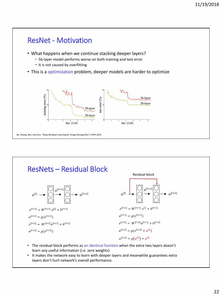
ResNet - Motivation

• What happens when we continue stacking deeper layers?− 56-layer model performs worse on both training and test error

− It is not caused by overfitting

• This is a optimization problem, deeper models are harder to optimize

He, Zhang, Ren, and Sun, “Deep Residual Learning for Image Recognition”, CVPR 2015

ResNets – Residual Block

𝑎[𝑙] 𝑎[𝑙+2]𝑎[𝑙+1]

𝑧[𝑙+2] = 𝑊[𝑙+2]𝑎[𝑙+1] + 𝑏[𝑙+2]

𝑎[𝑙+2] = 𝑔(𝑧[𝑙+2])

𝑎[𝑙] 𝑎[𝑙+2]𝑎[𝑙+1]

𝑧[𝑙+2] = 𝑊[𝑙+2]𝑎[𝑙+1] + 𝑏[𝑙+2]

𝑎[𝑙+2] = 𝑔(𝑧 𝑙+2 + 𝑎[𝑙])

𝑎[𝑙+2] = 𝑔 𝑎 𝑙 = 𝑎 𝑙

Residual block

• The residual block performs as an identical function when the extra two layers doesn’t learn any useful information (i.e. zero weights)

• It makes the network easy to learn with deeper layers and meanwhile guarantees extra layers don’t hurt network’s overall performance.

𝑧[𝑙+1] = 𝑊 [𝑙+1] 𝑎[𝑙] + 𝑏[𝑙+1]

𝑎[𝑙+1] = 𝑔(𝑧[𝑙+1])

𝑧[𝑙+1] = 𝑊 [𝑙+1] 𝑎[𝑙] + 𝑏[𝑙+1]

𝑎[𝑙+1] = 𝑔(𝑧[𝑙+1])

11/19/2018

23

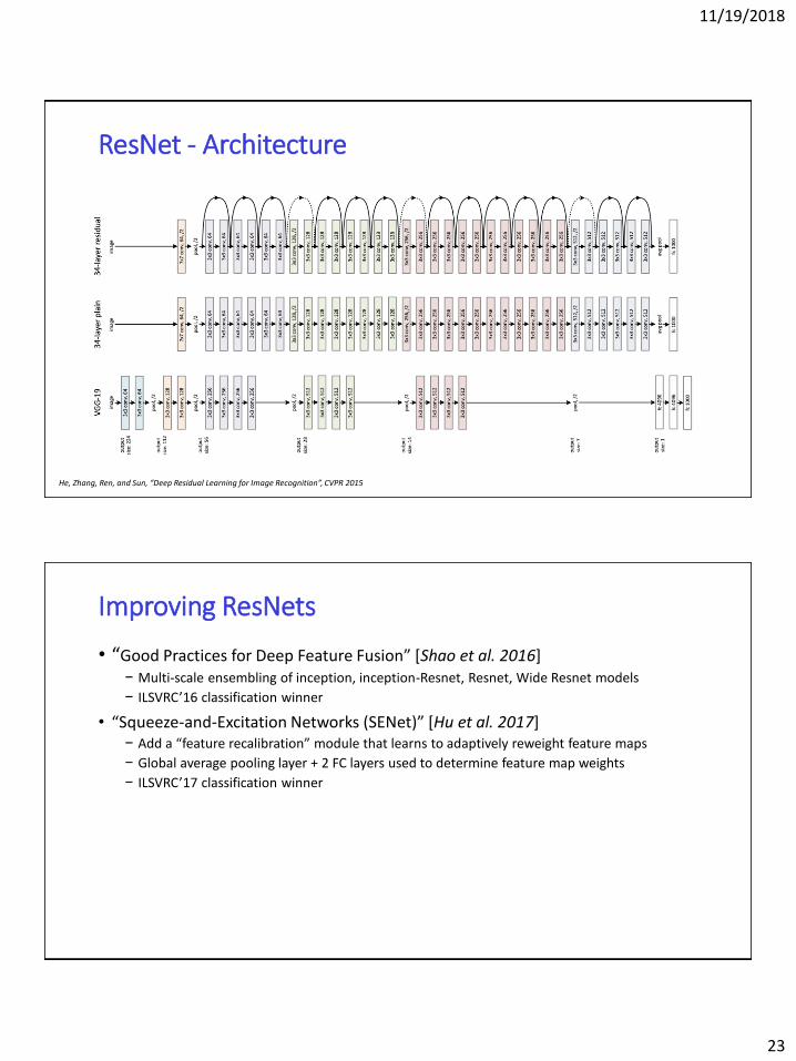
ResNet - Architecture

He, Zhang, Ren, and Sun, “Deep Residual Learning for Image Recognition”, CVPR 2015

Improving ResNets

• “Good Practices for Deep Feature Fusion” [Shao et al. 2016]− Multi-scale ensembling of inception, inception-Resnet, Resnet, Wide Resnet models

− ILSVRC’16 classification winner

• “Squeeze-and-Excitation Networks (SENet)” [Hu et al. 2017]− Add a “feature recalibration” module that learns to adaptively reweight feature maps

− Global average pooling layer + 2 FC layers used to determine feature map weights

− ILSVRC’17 classification winner

11/19/2018

24

Transfer Learning

• In practice, it is rare to have a dataset of sufficient size to train an entire convolutional network from scratch.

• Pertain a CNN trained on a very large dataset (e.g. ImageNet) and use it to a related new task.

• Transfer Learning scenarios− When new dataset is small and similar to original dataset

• Fixed Feature extractor: remove last classifier layer and treat the rest of the CNN as a fixed feature extractor for the new dataset.

− When new dataset is large and similar to original dataset• Fine-Tuning the CNN: not only replace and retrain the last classifier, but also fine-tune all the layers, or keep

some of the earlier layers fixed and only fine-tune some deeper portion of the network

− When new dataset is large different from the original dataset• Weights initialization: It is very often still beneficial to initialize with weights from a pretrained model and then

fine-tune through the entire network.

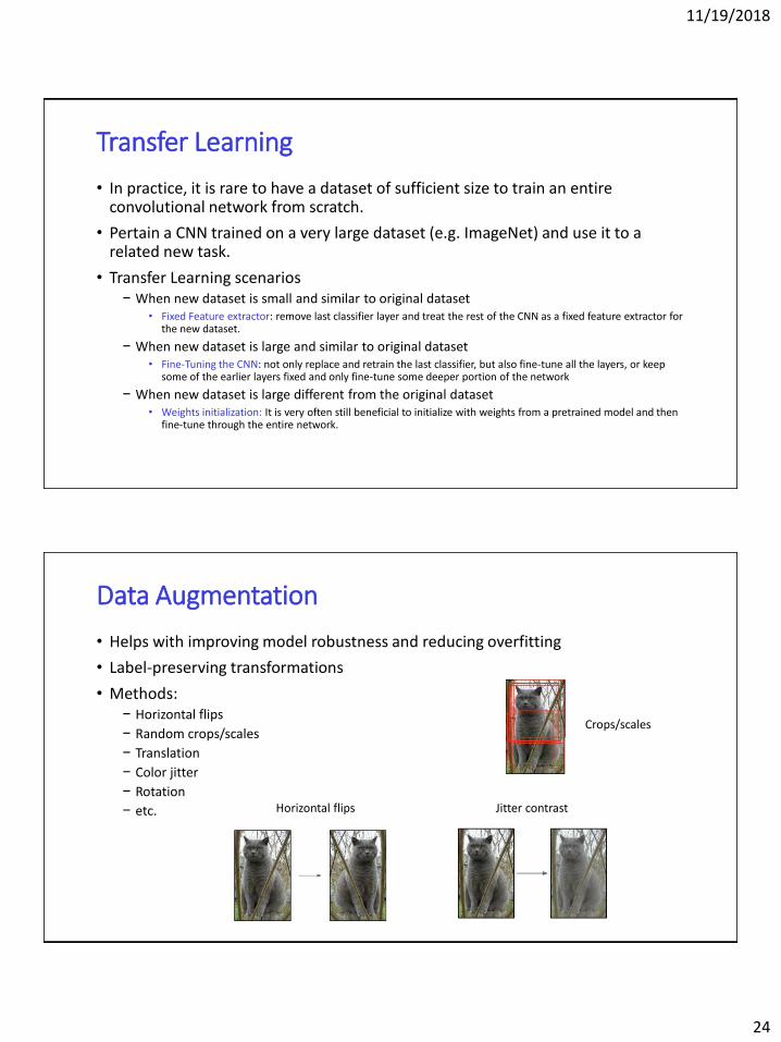
Data Augmentation

• Helps with improving model robustness and reducing overfitting

• Label-preserving transformations

• Methods:− Horizontal flips

− Random crops/scales

− Translation

− Color jitter

− Rotation

− etc. Horizontal flips

Crops/scales

Jitter contrast

11/19/2018

25

Convolutional Neural NetworkVisualizing and Understanding

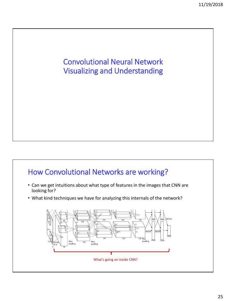
How Convolutional Networks are working?

• Can we get intuitions about what type of features in the images that CNN are looking for?

• What kind techniques we have for analyzing this internals of the network?

What’s going on inside CNN?

11/19/2018

26

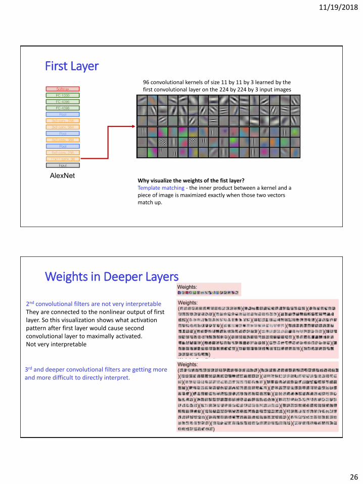
First Layer96 convolutional kernels of size 11 by 11 by 3 learned by the first convolutional layer on the 224 by 224 by 3 input images

Why visualize the weights of the fist layer?Template matching - the inner product between a kernel and a piece of image is maximized exactly when those two vectors match up.

Weights in Deeper Layers

2nd convolutional filters are not very interpretableThey are connected to the nonlinear output of first layer. So this visualization shows what activation pattern after first layer would cause second convolutional layer to maximally activated. Not very interpretable

3rd and deeper convolutional filters are getting more and more difficult to directly interpret.

11/19/2018

27

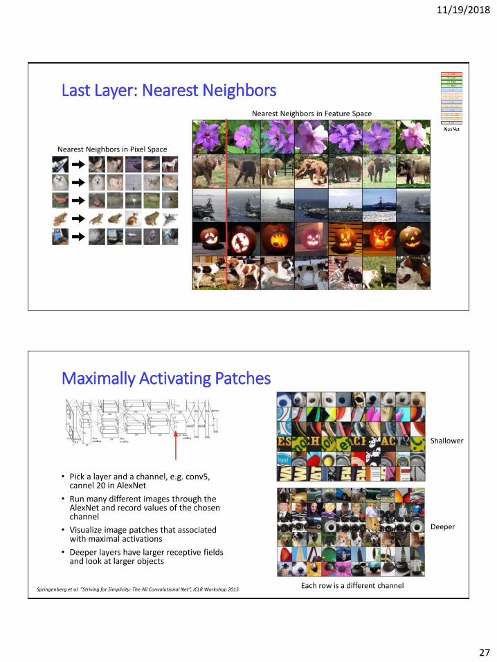
Last Layer: Nearest Neighbors

Nearest Neighbors in Pixel Space

Nearest Neighbors in Feature Space

Maximally Activating Patches

• Pick a layer and a channel, e.g. conv5, cannel 20 in AlexNet

• Run many different images through the AlexNet and record values of the chosen channel

• Visualize image patches that associated with maximal activations

• Deeper layers have larger receptive fields and look at larger objects

Each row is a different channelSpringenberg et al. “Striving for Simplicity: The All Convolutional Net”, ICLR Workshop 2015

Deeper

Shallower

11/19/2018

28

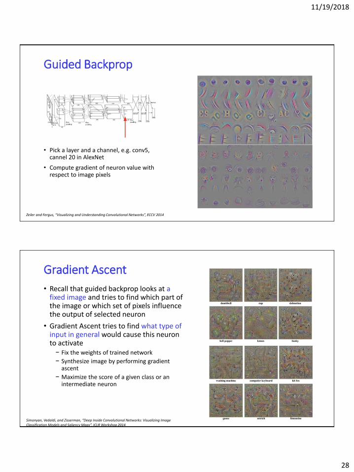
Guided Backprop

• Pick a layer and a channel, e.g. conv5, cannel 20 in AlexNet

• Compute gradient of neuron value with respect to image pixels

Zeiler and Fergus, “Visualizing and Understanding Convolutional Networks”, ECCV 2014

Gradient Ascent

• Recall that guided backprop looks at a fixed image and tries to find which part of the image or which set of pixels influence the output of selected neuron

• Gradient Ascent tries to find what type of input in general would cause this neuron to activate− Fix the weights of trained network

− Synthesize image by performing gradient ascent

− Maximize the score of a given class or an intermediate neuron

Simonyan, Vedaldi, and Zisserman, “Deep Inside Convolutional Networks: Visualizing Image Classification Models and Saliency Maps”, ICLR Workshop 2014

11/19/2018

29

More Applications

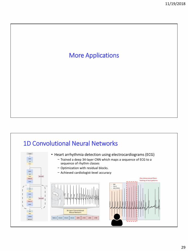
1D Convolutional Neural Networks

• Heart arrhythmia detection using electrocardiograms (ECG)− Trained a deep 34-layer CNN which maps a sequence of ECG to a

sequence of rhythm classes

− Optimization with residual blocks.

− Achieved cardiologist-level accuracy

One dimensional filters looking at local patterns

11/19/2018

30

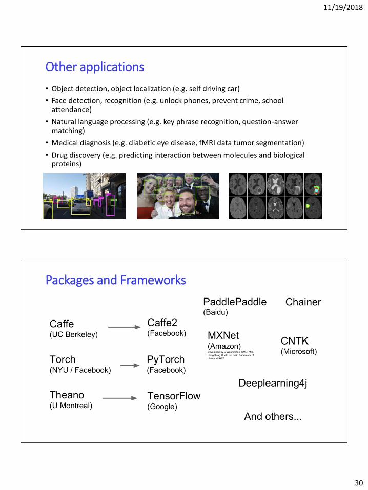
Other applications

• Object detection, object localization (e.g. self driving car)

• Face detection, recognition (e.g. unlock phones, prevent crime, school attendance)

• Natural language processing (e.g. key phrase recognition, question-answer matching)

• Medical diagnosis (e.g. diabetic eye disease, fMRI data tumor segmentation)

• Drug discovery (e.g. predicting interaction between molecules and biological proteins)

Packages and Frameworks

11/19/2018

31

References

• Gradient-Based Learning Applied to Document Recognition, LeCun, Bottou, Bengio, Haffner, IEEE 1998

• ImageNet Classification with Deep Convolutional Neural Networks, Krizhevsky, Sutskever, Hinton, NIPS 2012

• Very Deep Convolutional Networks For Large-Scale Image Recognition, Simonyan, Zisserman, ICLR 2015

• Deep Residual Learning for Image Recognition, He, Zhang, Ren, and Sun, CVPR 2015

• Good Practices for Deep Feature Fusion, Shao et al. 2016

• Squeeze-and-Excitation Networks (SENet), Hu et al. CVPR 2017

• Striving for Simplicity: The All Convolutional Net, Springenberg et al., ICLR Workshop 2015

• Visualizing and Understanding Convolutional Networks, Zeiler and Fergus, ECCV 2014

• Deep Inside Convolutional Networks: Visualizing Image Classification Models and Saliency Maps, Simonyan, Vedaldi, and Zisserman, ICLR Workshop 2014

Tutorials

• Stanford CS231n: Convolutional Neural Networks for Visual Recognition

• Coursera Deep Learning Specialization

• CMU 11777, Lecture 3: CNN and Optimization

11/19/2018

32

Thank You!Q & A