convolution discrete and continuous time-difference equaion and system properties (1)
TRANSCRIPT
Discrete Time Signals
Convolution of Discrete Time Signals
Properties of the Systems
B.S. Panwar
Convolve: It is latin word which means fold over or twisting together

Sampling Property
Continuous Time
&
Discrete Time
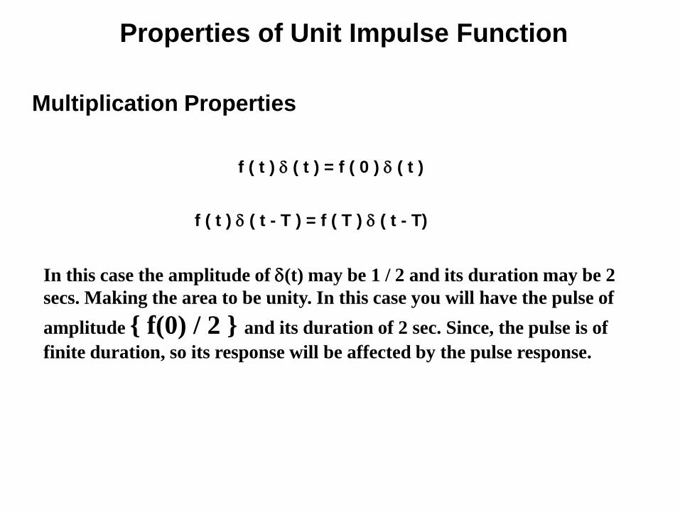
Properties of Unit Impulse Function
f ( t ) ( t ) = f ( 0 ) ( t )
f ( t ) ( t - T ) = f ( T ) ( t - T)
Multiplication Properties
In this case the amplitude of (t) may be 1 / 2 and its duration may be 2
secs. Making the area to be unity. In this case you will have the pulse of
amplitude { f(0) / 2 } and its duration of 2 sec. Since, the pulse is of
finite duration, so its response will be affected by the pulse response.
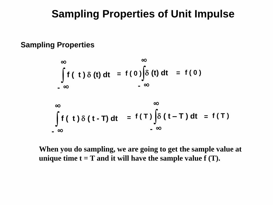
Sampling Properties of Unit Impulse
Sampling Properties
=∫- ∞
f ( t ) (t) dt
∞=∫
- ∞
(t) dt
∞
f ( 0 ) f ( 0 )
=∫- ∞
f ( t ) ( t - T) dt
∞=∫
- ∞
( t – T ) dt
∞
f ( T ) f ( T )
When you do sampling, we are going to get the sample value at
unique time t = T and it will have the sample value f (T).
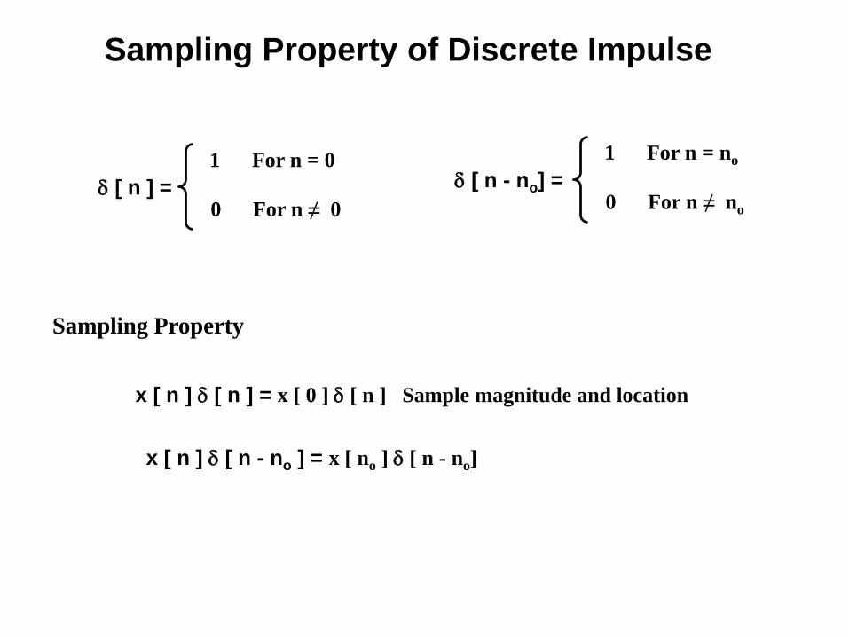
Sampling Property of Discrete Impulse
[ n ] =
1 For n = 0
0 For n ≠ 0
[ n - no] =
1 For n = no
0 For n ≠ no
x [ n ] [ n ] = x [ 0 ] [ n ] Sample magnitude and location
x [ n ] [ n - no ] = x [ no ] [ n - no]
Sampling Property
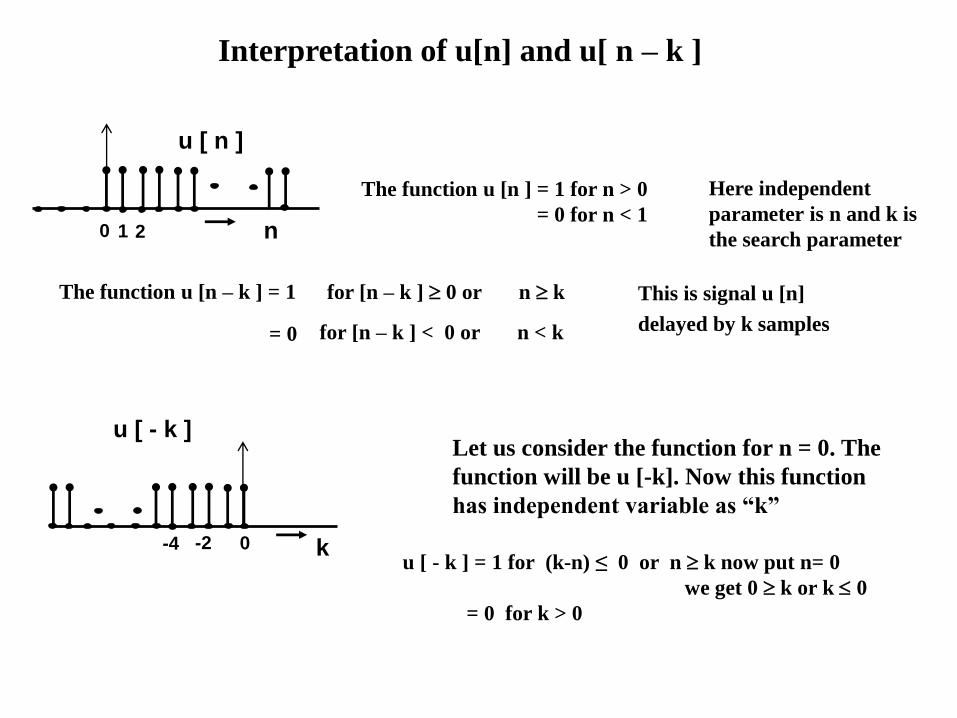
Interpretation of u[n] and u[ n – k ]
n
u [ n ]
0 1 2
k
u [ - k ]
0-4 -2
The function u [n ] = 1 for n > 0
= 0 for n < 1
The function u [n – k ] = 1 for [n – k ] 0 or n k
= 0 for [n – k ] < 0 or n < k
u [ - k ] = 1 for (k-n) ≤ 0 or n k now put n= 0
we get 0 k or k 0
= 0 for k > 0
Let us consider the function for n = 0. The
function will be u [-k]. Now this function
has independent variable as “k”
This is signal u [n]
delayed by k samples
Here independent
parameter is n and k is
the search parameter
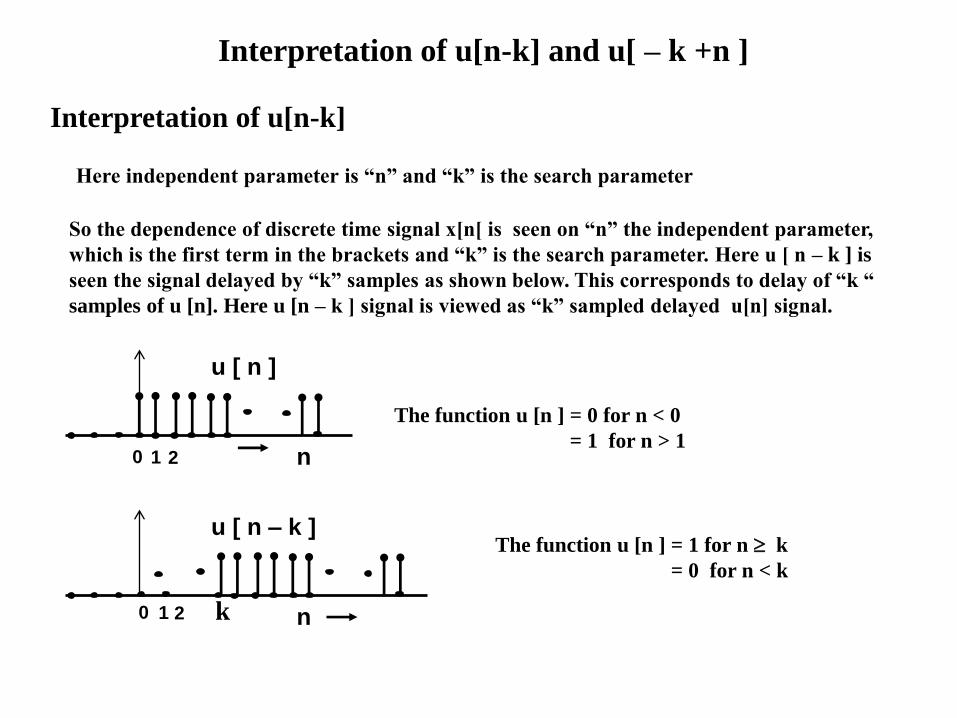
Interpretation of u[n-k] and u[ – k +n ]
Here independent parameter is “n” and “k” is the search parameter
So the dependence of discrete time signal x[n[ is seen on “n” the independent parameter,
which is the first term in the brackets and “k” is the search parameter. Here u [ n – k ] is
seen the signal delayed by “k” samples as shown below. This corresponds to delay of “k “
samples of u [n]. Here u [n – k ] signal is viewed as “k” sampled delayed u[n] signal.
n
u [ n – k ]
0 1 2
The function u [n ] = 1 for n k
= 0 for n < k
k
n
u [ n ]
0 1 2
The function u [n ] = 0 for n < 0
= 1 for n > 1
Interpretation of u[n-k]
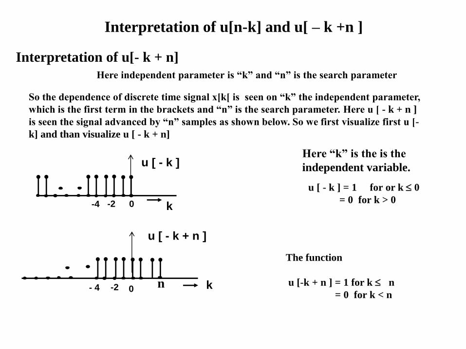
Interpretation of u[n-k] and u[ – k +n ]
k
u [ - k ]
0-4 -2
u [ - k ] = 1 for or k 0
= 0 for k > 0
Here “k” is the is the
independent variable.
Here independent parameter is “k” and “n” is the search parameter
So the dependence of discrete time signal x[k[ is seen on “k” the independent parameter,
which is the first term in the brackets and “n” is the search parameter. Here u [ - k + n ]
is seen the signal advanced by “n” samples as shown below. So we first visualize first u [-
k] and than visualize u [ - k + n]
Interpretation of u[- k + n]
k
u [ - k + n ]
-2 0
The function
u [-k + n ] = 1 for k n
= 0 for k < n n- 4
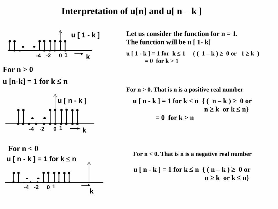
Interpretation of u[n] and u[ n – k ]
u [ 1 - k ] = 1 for k 1 ( ( 1 – k ) 0 or 1 k )
= 0 for k > 1
Let us consider the function for n = 1.
The function will be u [ 1- k]
k
u [ 1 - k ]
0-4 -2 1
k
u [ n - k ]
0-4 -2 1
For n > 0. That is n is a positive real number
u [ n - k ] = 1 for k < n { ( n – k ) 0 or
n k or k n}
= 0 for k > n
k0-4 -2 1
For n > 0
u [ n - k ] = 1 for k n
For n < 0For n < 0. That is n is a negative real number
u [ n - k ] = 1 for k n { ( n – k ) 0 or
n k or k n}
u [n-k] = 1 for k n
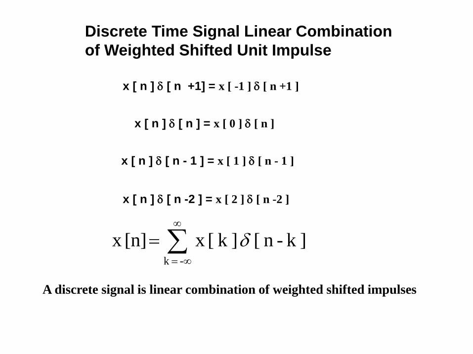
Discrete Time Signal Linear Combination
of Weighted Shifted Unit Impulse
x [ n ] [ n +1] = x [ -1 ] [ n +1 ]
x [ n ] [ n ] = x [ 0 ] [ n ]
x [ n ] [ n - 1 ] = x [ 1 ] [ n - 1 ]
x [ n ] [ n -2 ] = x [ 2 ] [ n -2 ]
- k
]k -n [ ]k [ x [n]x
A discrete signal is linear combination of weighted shifted impulses
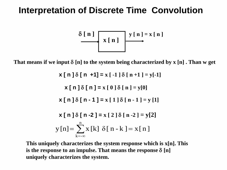
Interpretation of Discrete Time Convolution
y [ n ] = x [ n ] [ n ]x [ n ]
]n[x]k -n [ δ [k]x [n]y n
-k
That means if we input [n] to the system being characterized by x [n] . Than w get
x [ n ] [ n +1] = x [ -1 ] [ n +1 ] = y[-1]
x [ n ] [ n ] = x [ 0 ] [ n ] = y[0]
x [ n ] [ n - 1 ] = x [ 1 ] [ n - 1 ] = y [1]
x [ n ] [ n -2 ] = x [ 2 ] [ n -2 ] = y[2]
This uniquely characterizes the system response which is x[n]. This
is the response to an impulse. That means the response [n]
uniquely characterizes the system.
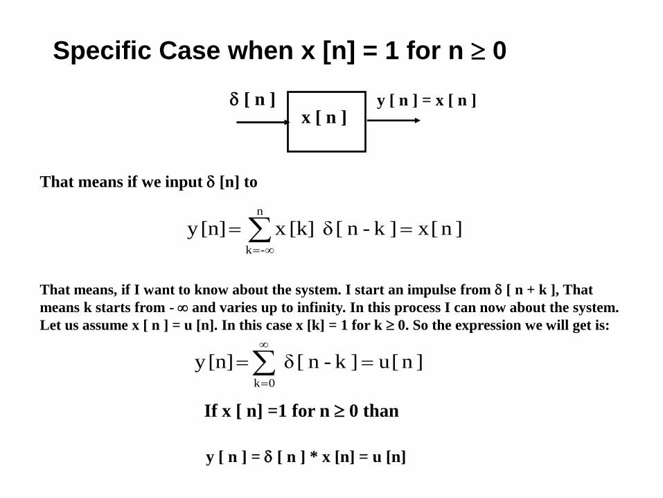
Specific Case when x [n] = 1 for n 0
]n[u]k -n [ δ [n]y 0k
y [ n ] = [ n ] * x [n] = u [n]
y [ n ] = x [ n ] [ n ]x [ n ]
That means, if I want to know about the system. I start an impulse from [ n + k ], That
means k starts from - and varies up to infinity. In this process I can now about the system.
Let us assume x [ n ] = u [n]. In this case x [k] = 1 for k 0. So the expression we will get is:
]n[x]k -n [ δ [k]x [n]y n
-k
If x [ n] =1 for n 0 than
That means if we input [n] to
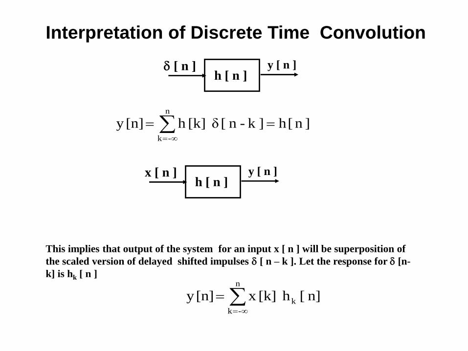
y [ n ] [ n ]h [ n ]
]n[h]k -n [ δ [k]h [n]y n
-k
Interpretation of Discrete Time Convolution
y [ n ]x [ n ]h [ n ]
n
-k
k n] [ h [k]x [n]y
This implies that output of the system for an input x [ n ] will be superposition of
the scaled version of delayed shifted impulses [ n – k ]. Let the response for [n-
k] is hk [ n ]
Interpretation of Discrete Time Convolution
n
-k
k n] [ h [k]x [n]y
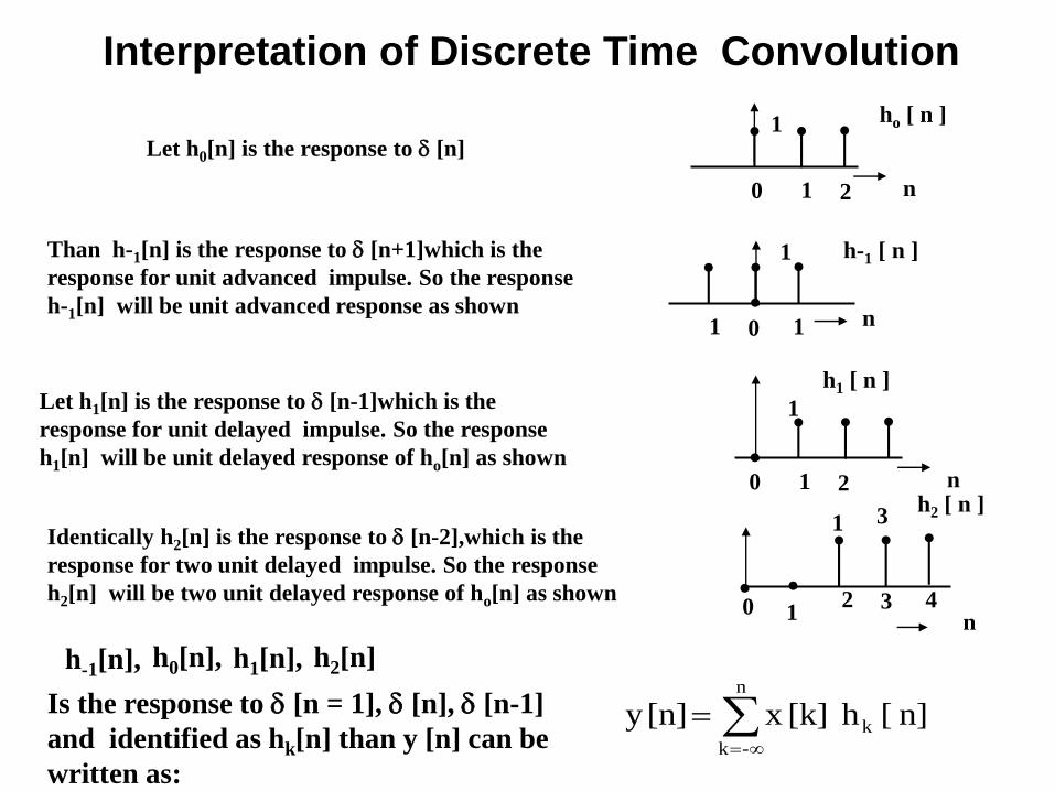
Let h0[n] is the response to [n]
0 1
1 ho [ n ]
n2
Than h-1[n] is the response to [n+1]which is the
response for unit advanced impulse. So the response
h-1[n] will be unit advanced response as shown1
1 h-1 [ n ]
n0 1
0 2
1h2 [ n ]
n3 4
1
Let h1[n] is the response to [n-1]which is the
response for unit delayed impulse. So the response
h1[n] will be unit delayed response of ho[n] as shown
3
0 1
1
h1 [ n ]
n2
Identically h2[n] is the response to [n-2],which is the
response for two unit delayed impulse. So the response
h2[n] will be two unit delayed response of ho[n] as shown
h-1[n], h0[n], h1[n], h2[n]
Is the response to [n = 1], [n], [n-1]
and identified as hk[n] than y [n] can be
written as:
Interpretation of Discrete Time Convolution
n
-k
k n] [ h [k]x [n]y
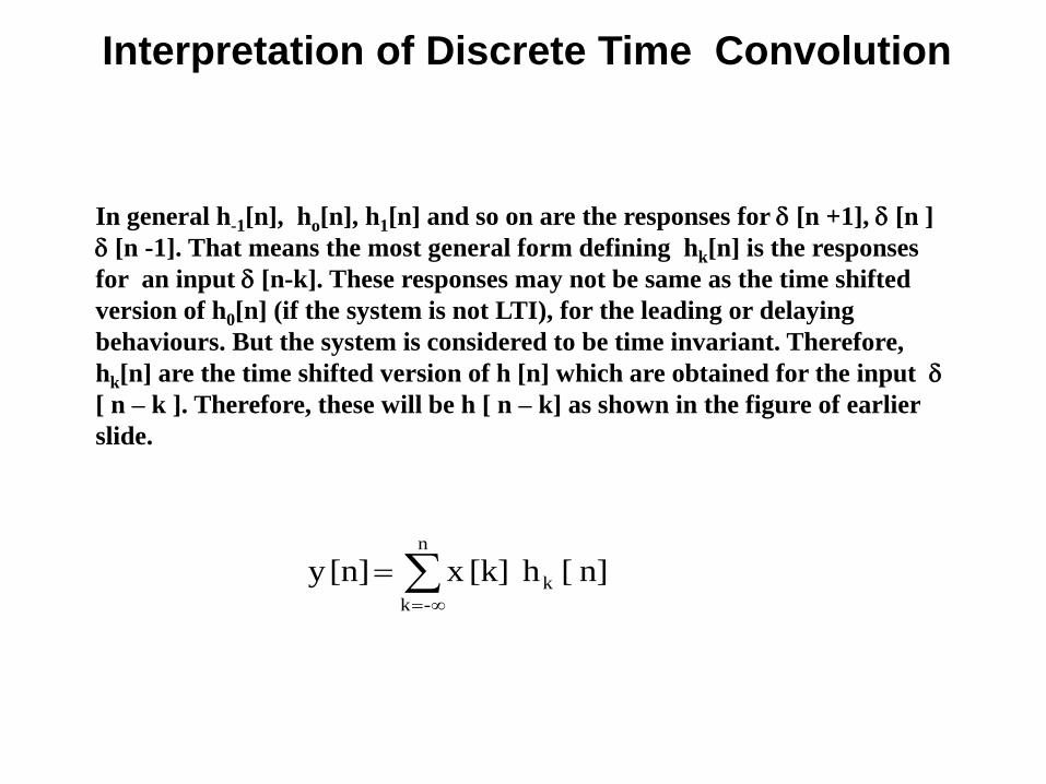
In general h-1[n], ho[n], h1[n] and so on are the responses for [n +1], [n ]
[n -1]. That means the most general form defining hk[n] is the responses
for an input [n-k]. These responses may not be same as the time shifted
version of h0[n] (if the system is not LTI), for the leading or delaying
behaviours. But the system is considered to be time invariant. Therefore,
hk[n] are the time shifted version of h [n] which are obtained for the input
[ n – k ]. Therefore, these will be h [ n – k] as shown in the figure of earlier
slide.
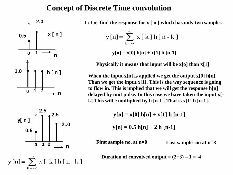
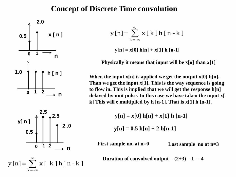
Concept of Discrete Time convolution
n0 1
x [ n ] 0.5
2.0
n0 1 2
h [ n ]
- k
]k -n [h ]k [ x [n]y
y[n] = x[0] h[n] + x[1] h [n-1]
y[n] = 0.5 h[n] + 2 h [n-1]
When the input x[n] is applied we get the output x[0] h[n].
Than we get the input x[1]. This is the way sequence is going
to flow in. This is implied that we will get the response h[n]
delayed by unit pulse. In this case we have taken the input x[-
k] This will e multiplied by h [n-1]. That is x[1] h [n-1].
y[n] = x[0] h[n] + x[1] h [n-1]
Physically it means that input will be x[o] than x[1]
First sample no. at n=0 Last sample no at n=3
Duration of convolved output = (2+3) – 1 = 4
1.0
n0 1 2
y[ n ]
0.5
2.52.5
2..0
- k
]k -n [h ]k [ x [n]y
Let us find the response for x [ n ] which has only two samples
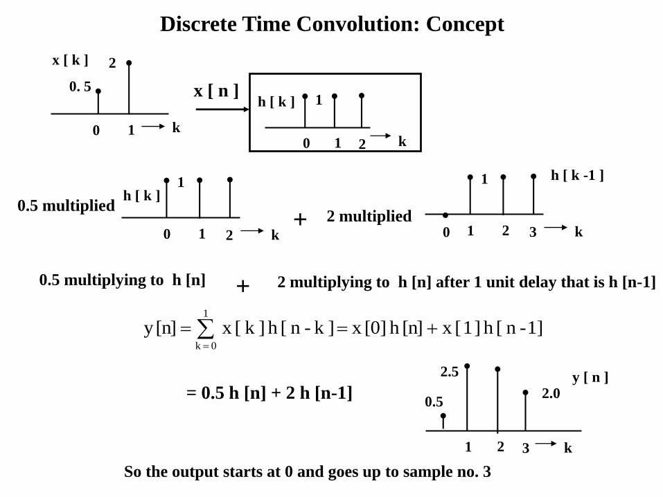
Discrete Time Convolution: Concept
0 1
0. 5
2x [ k ]
k
1]-n [h ] 1 [ x [n]h [0] x ]k -n [h ]k [ x [n]y 1
0 k
= 0.5 h [n] + 2 h [n-1]
0 1
1h [ k ]
k2
x [ n ]
0 1
1h [ k ]
k2
2 multiplied
0.5 multiplying to h [n]
+
+ 2 multiplying to h [n] after 1 unit delay that is h [n-1]
0.5 multiplied
1 2
1 h [ k -1 ]
k30
1 2
2.5 y [ n ]
k3
0.52.0
So the output starts at 0 and goes up to sample no. 3

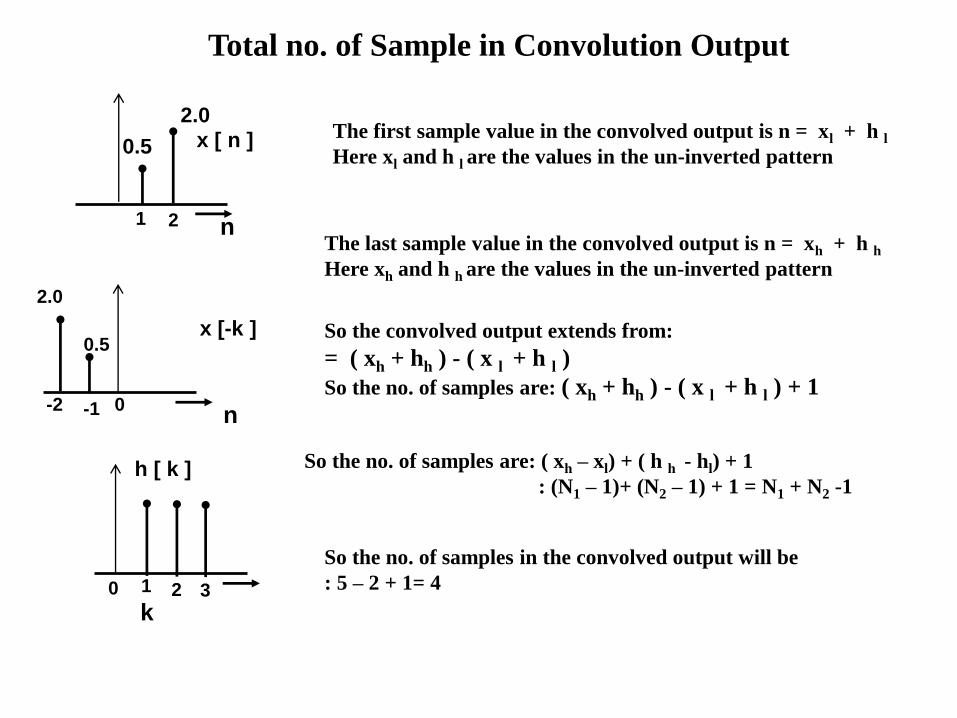
Total no. of Sample in Convolution Output
n1 2
x [ n ] 0.5
2.0
k0 1 2
h [ k ]
3
n0-2
x [-k ] 0.5
2.0
-1
So the no. of samples in the convolved output will be
: 5 – 2 + 1= 4
The last sample value in the convolved output is n = xh + h hHere xh and h h are the values in the un-inverted pattern
So the no. of samples are: ( xh – xl) + ( h h - hl) + 1
: (N1 – 1)+ (N2 – 1) + 1 = N1 + N2 -1
So the convolved output extends from sample no.:
= ( xh + hh ) - ( x l + h l )
So the no. of samples are: ( xh + hh ) - ( x l + h l ) + 1
The first sample value in the convolved output is n = xl + h lHere xl and h l are the values in the un-inverted pattern
Discrete Time Convolution

First and Last Sample Value
in the Convolved Output
Total no. of Sample in Convolution Output
n1 2
x [ n ] 0.5
2.0
k0 1 2
h [ k ]
3
n0-2
x [-k ] 0.5
2.0
-1
So the no. of samples in the convolved output will be
: 5 – 2 + 1= 4
The last sample value in the convolved output is n = xh + h hHere xh and h h are the values in the un-inverted pattern
So the no. of samples are: ( xh – xl) + ( h h - hl) + 1
: (N1 – 1)+ (N2 – 1) + 1 = N1 + N2 -1
So the convolved output extends from:
= ( xh + hh ) - ( x l + h l )
So the no. of samples are: ( xh + hh ) - ( x l + h l ) + 1
The first sample value in the convolved output is n = xl + h lHere xl and h l are the values in the un-inverted pattern
Concept of Discrete Time convolution
n0 1
x [ n ] 0.5
2.0
n0 1 2
h [ n ]
- k
]k -n [h ]k [ x [n]y
y[n] = x[0] h[n] + x[1] h [n-1]
y[n] = 0.5 h[n] + 2 h[n-1]
When the input x[n] is applied we get the output x[0] h[n].
Than we get the input x[1]. This is the way sequence is going
to flow in. This is implied that we will get the response h[n]
delayed by unit pulse. In this case we have taken the input x[-
k] This will e multiplied by h [n-1]. That is x[1] h [n-1].
y[n] = x[0] h[n] + x[1] h [n-1]
Physically it means that input will be x[o] than x[1]
First sample no. at n=0 Last sample no at n=3
Duration of convolved output = (2+3) – 1 = 4
1.0
n0 1 2
y[ n ]
0.5
2.52.5
2..0
- k
]k -n [h ]k [ x [n]y
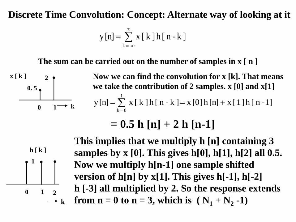
Discrete Time Convolution: Concept: Alternate way of looking at it
- k
]k -n [h ]k [ x [n]y
The sum can be carried out on the number of samples in x [ n ]
0 1
0. 5
2x [ k ]
k
Now we can find the convolution for x [k]. That means
we take the contribution of 2 samples. x [0] and x[1]
1]-n [h ] 1 [ x [n]h [0] x ]k -n [h ]k [ x [n]y 1
0 k
This implies that we multiply h [n] containing 3
samples by x [0]. This gives h[0], h[1], h[2] all 0.5.
Now we multiply h[n-1] one sample shifted
version of h[n] by x[1]. This gives h[-1], h[-2]
h [-3] all multiplied by 2. So the response extends
from n = 0 to n = 3, which is ( N1 + N2 -1)
= 0.5 h [n] + 2 h [n-1]
0 1
1
h [ k ]
k
2
0 1
2 3
x[n]
n
1
2
1
-1 0 1
h[n]
n
22
0 1 2
3
y[n]
n-1
4 5 6
2
4
2 2
-2
Convolution of Two Discrete Time Signals
The lower starting sample will be sum of
lowest sample points of two signals
- k k]-n [h [k]x [n]y
Commutative property
y[n] = x[0] h[n] + x[1] h [n-1] + x[2] h[n-2] + x[3] h[n-3]
- k k]-n [ x [k]h [n]y
This will give the output y [n] as:
y[n] = x[n+1] h[-1] + h[1] x [n-1]
The highest sample point will be sum of
highest sample points of two signalsTotal no. of samples will be the
sum of samples in both the
signals -1. That is N1 + N2 -1
Examples on Discrete
Time Convolution
n
h[n] =u [ n ]
0
h [ n ] = u [n]
k
h [ 0 - k ]
0
k
u [ 1 - k ]
0
k
u [-1 – k ]
0
n0 1 2
x [ n ]
- k
]k -n [h ]k [ x [n]y
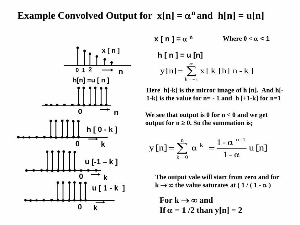
Here h[-k] is the mirror image of h [n]. And h[-
1-k] is the value for n= - 1 and h [+1-k] for n=1
Example Convolved Output for x[n] = n and h[n] = u[n]
We see that output is 0 for n < 0 and we get
output for n 0. So the summation is;
[n]u α - 1
α - 1 α [n]y
1nn
0 k
k
The output vale will start from zero and for
k the value saturates at ( 1 / ( 1 - )
x [ n ] = n Where 0 < < 1
For k and
If = 1 /2 than y[n] = 2
k
h [ - k ]
0
k 0-1-2
x [ k ]
Convolved Output for x[n] = 2n u[-n] and h[n] = u[n]
0
- k
k 2 [n]y
If we change the variable k = -m. We get the
integral from 0 to . This is when we are
computing only for n ranging from - to 0
2 1/2) - 1 (
1
2
1 [n]y
0 k
k
However we need to compute
the integral in the entire range
of “n” for which we get:
n
- k
k 2 [n]y If k we replace k by k = - k
n - k
k 2
1 [n]y If k we replace k by
k + n = m, we get
2
1 2
2
1 [n]y
0 m
m
n
0 m
n-m
1 n2 [n]y or
x[k] starts the output at - and
h[k] leads the output until . So
the output is from - to
Now considering the complete output from -
to n, where will also tend to infinity
The summation taken from - to 0 will show
that the output it must saturate at n=0

n
h [ n ]
0
h [ n ] = u [ - n]
k
h [ -k ]
0
k
u [ 1 - k ]
0
k0 1 2
x [ k ]
- k
]k -n [h ]k [ x [n]y
Here h[-k] is the mirror image of h [n]. And h[-
1-k] is the value for n= - 1 and h [+1-k] for n=1
Example Convolved Output for x[n] = n and h[n] = u[-n]
We see that output is 0 for n < 0 and we get
output for n 0. So the summation is;
[n]u α - 1
α - 1 α [n]y
1nn
0 k
k
The output vale will start from zero and for
k the value saturates at ( 1 / ( 1 - )
x [ n ] = n Where 0 < < 1
k0
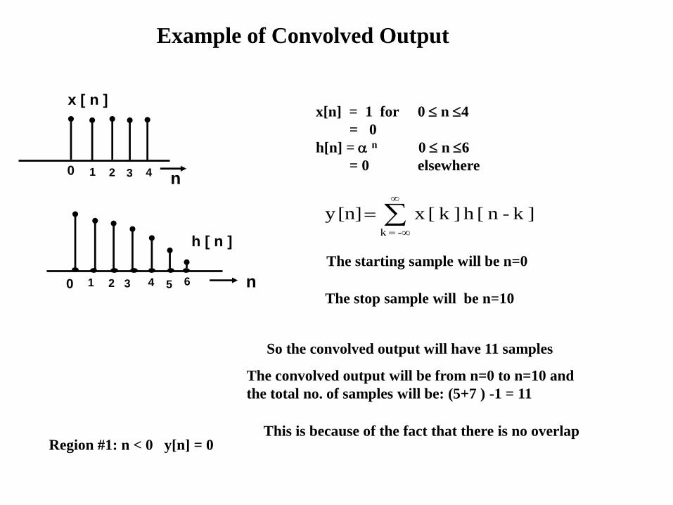
Example of Convolved Output
x[n] = 1 for 0 n 4
= 0
h[n] = n 0 n 6
= 0 elsewhere
- k
]k -n [h ]k [ x [n]y
The convolved output will be from n=0 to n=10 and
the total no. of samples will be: (5+7 ) -1 = 11
Region #1: n < 0 y[n] = 0
n0 1 2
x [ n ]
3 4
n
h [ n ]
0 1 2 3 4 5 6
The starting sample will be n=0
The stop sample will be n=10
This is because of the fact that there is no overlap
So the convolved output will have 11 samples
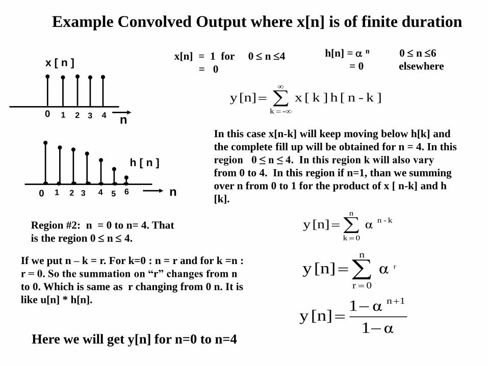
Example Convolved Output where x[n] is of finite duration
x[n] = 1 for 0 n 4
= 0
- k
]k -n [h ]k [ x [n]y
In this case x[n-k] will keep moving below h[k] and
the complete fill up will be obtained for n = 4. In this
region 0 ≤ n ≤ 4. In this region k will also vary
from 0 to 4. In this region if n=1, than we summing
over n from 0 to 1 for the product of x [ n-k] and h
[k].
Region #2: n = 0 to n= 4. That
is the region 0 n 4.
n
0 k
k -n α [n]y
n
0 r
rα [n]y
α1
α1 [n]y
1n
n0 1 2
x [ n ]
3 4
n
h [ n ]
0 1 2 3 4 5 6
h[n] = n 0 n 6
= 0 elsewhere
If we put n – k = r. For k=0 : n = r and for k =n :
r = 0. So the summation on “r” changes from n
to 0. Which is same as r changing from 0 n. It is
like u[n] * h[n].
Here we will get y[n] for n=0 to n=4
k
h [ k ]
0 1 2 3 4 5 6
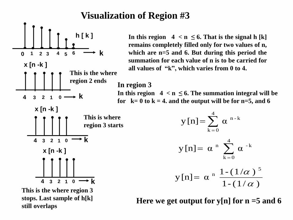
Visualization of Region #3
k
x [n -k ]
4 3 2 1 0
This is the where
region 2 ends
This is where
region 3 starts
This is the where region 3
stops. Last sample of h[k]
still overlaps
In this region 4 < n ≤ 6. That is the signal h [k]
remains completely filled only for two values of n,
which are n=5 and 6. But during this period the
summation for each value of n is to be carried for
all values of “k”, which varies from 0 to 4.
In region 3In this region 4 < n ≤ 6. The summation integral will be
for k= 0 to k = 4. and the output will be for n=5, and 6
4
0 k
k -n α [n]y
Here we get output for y[n] for n =5 and 6
4
0 k
k -n α α [n]y
) / 1 ( - 1
) /1 ( - 1 α [n]y
5n
k
x [n -k ]
4 3 2 1 0
k
x [n -k ]
4 3 2 1 0
k
h [ k ]
0 1 2 3 4 5 6
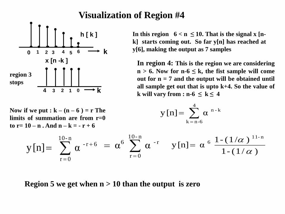
Visualization of Region #4
region 3
stops
In this region 6 < n ≤ 10. That is the signal x [n-
k] starts coming out. So far y[n] has reached at
y[6], making the output as 7 samples
In region 4: This is the region we are considering
n > 6. Now for n-6 ≤ k, the fist sample will come
out for n = 7 and the output will be obtained until
all sample get out that is upto k+4. So the value of
k will vary from : n-6 ≤ k ≤ 4
4
6-n k
k -n α [n]y
Region 5 we get when n > 10 than the output is zero
n - 10
0 r
6 r - α [n]y ) / 1 ( - 1
) /1 ( - 1 α [n]y
n - 11 6
k
x [n -k ]
4 3 2 1 0
Now if we put : k – (n – 6 ) = r The
limits of summation are from r=0
to r= 10 – n . And n – k = - r + 6
n - 10
0 r
r - 6 α α
Correlation / Correlation
Between Two Signals(continuous time)
f1()
f2()
T
∫-∞
∞
f1 ( ) f2 ( ) d
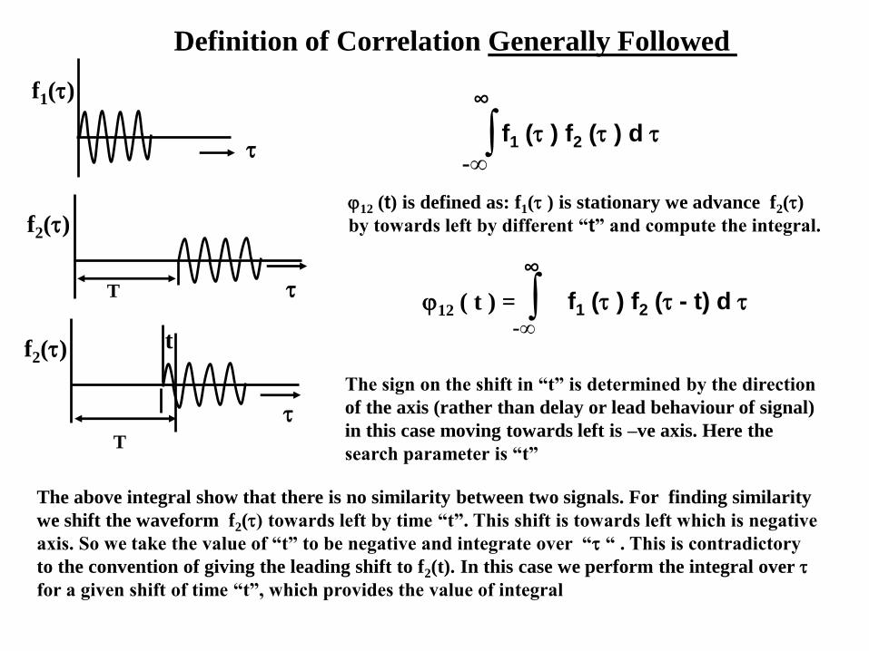
Definition of Correlation Generally Followed
The above integral show that there is no similarity between two signals. For finding similarity
we shift the waveform f2() towards left by time “t”. This shift is towards left which is negative
axis. So we take the value of “t” to be negative and integrate over “ “ . This is contradictory
to the convention of giving the leading shift to f2(t). In this case we perform the integral over
for a given shift of time “t”, which provides the value of integral
∫-∞
∞
f1 ( ) f2 ( - t) d 12 ( t ) =
12 (t) is defined as: f1() is stationary we advance f2()
by towards left by different “t” and compute the integral.
f2()
T
t
The sign on the shift in “t” is determined by the direction
of the axis (rather than delay or lead behaviour of signal)
in this case moving towards left is –ve axis. Here the
search parameter is “t”
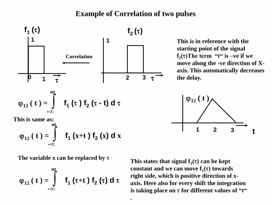
Example of Correlation of two pulses
f1 ()
1
0 1
f2 ()
1
2 3
Correlation
This is in reference with the
starting point of the signal
f2()The term “t“ is –ve if we
move along the -ve direction of X-
axis. This automatically decreases
the delay.
t1 32
12 ( t )
This is same as:
∫-∞
∞
f1 ( ) f2 ( - t) d 12 ( t ) =
∫-∞
∞
f1 (x+t ) f2 (x) d x12 ( t ) =
∫-∞
∞
f1 (+t ) f2 () d 12 ( t ) =
The variable x can be replaced by This states that signal f2() can be kept
constant and we can move f1() towards
right side, which is positive direction of x-
axis. Here also for every shift the integration
is taking place on for different values of “t“
.
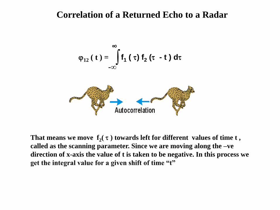
Correlation of a Returned Echo to a Radar
∫-∞
∞
f1 ( ) f2 ( - t ) d12 ( t ) =
That means we move f2( ) towards left for different values of time t ,
called as the scanning parameter. Since we are moving along the –ve
direction of x-axis the value of t is taken to be negative. In this process we
get the integral value for a given shift of time “t”
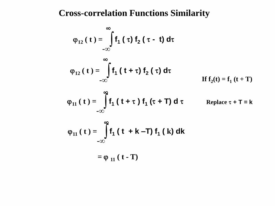
Cross-correlation Functions Similarity
∞
∫-∞
f1 ( t + ) f1 ( + T) d 11 ( t ) =
∫-∞
∞
f1 ( ) f2 ( - t) d12 ( t ) =
∫-∞
∞
f1 ( t + ) f2 ( ) d12 ( t ) =
∞
∫-∞
f1 ( t + k –T) f1 ( k) dk11 ( t ) =
Replace + T = k
= 11 ( t - T)
If f2(t) = f1 (t + T)
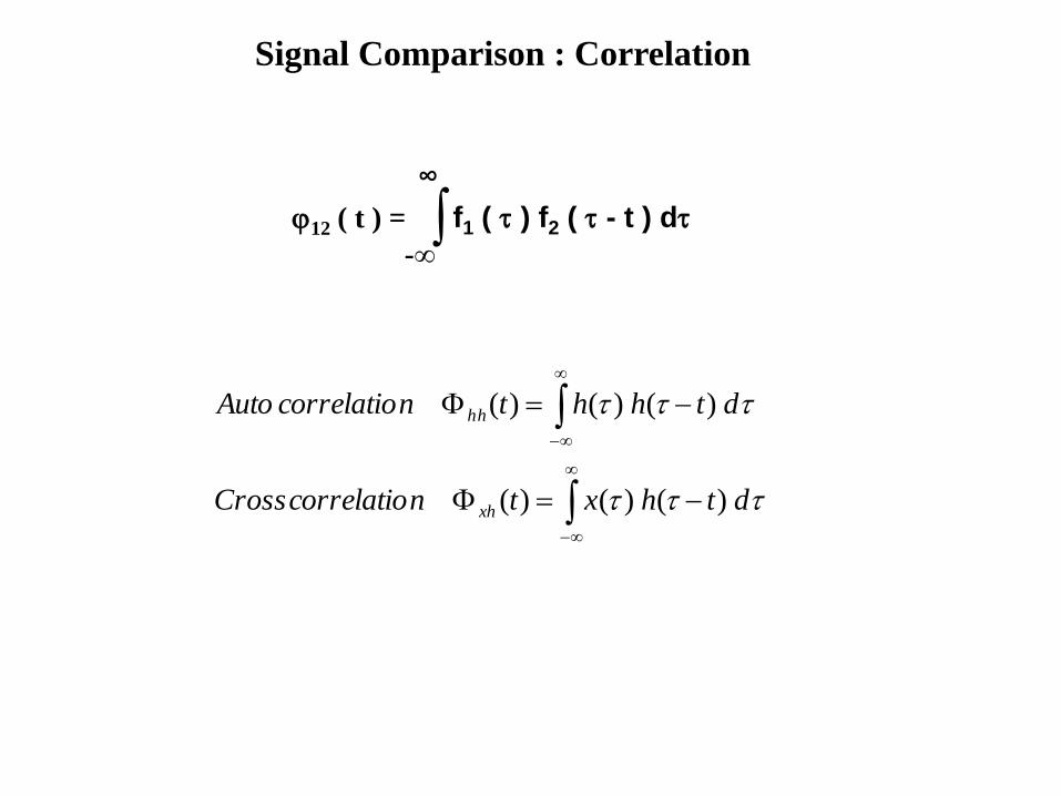
Signal Comparison : Correlation
∫-∞
∞
f1 ( ) f2 ( - t ) d12 ( t ) =
dthxtncorrelatioCross
dthhtncorrelatioAuto
xh
hh
)()()(
)()()(
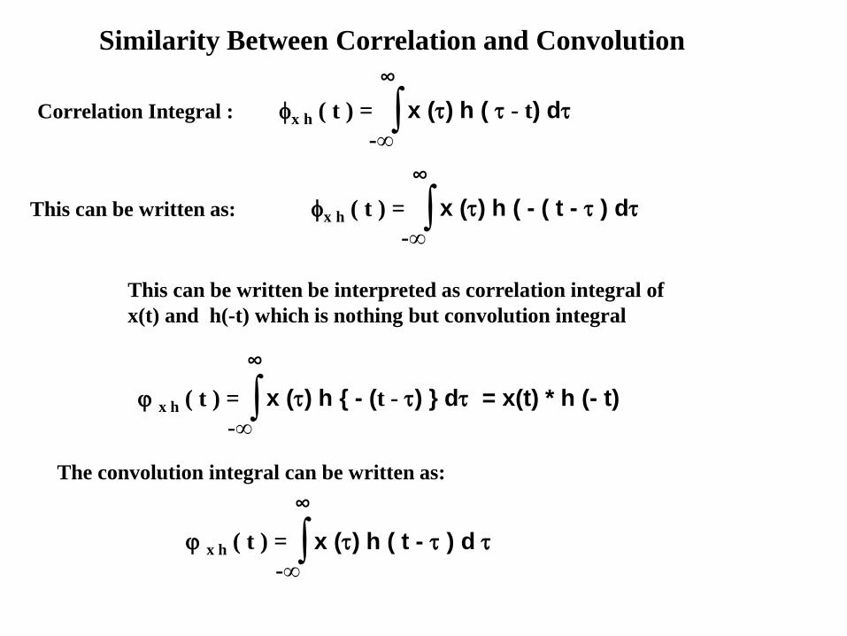
Similarity Between Correlation and Convolution
Correlation Integral : ∫-∞
∞
x () h ( - t) dx h ( t ) =
∞
∫-∞
x () h { - (t - ) } d = x(t) * h (- t) x h ( t ) =
∞
∫-∞
x () h ( t - ) d x h ( t ) =
This can be written as:
∞
∫-∞
x () h ( - ( t - ) dx h ( t ) =
This can be written be interpreted as correlation integral of
x(t) and h(-t) which is nothing but convolution integral
The convolution integral can be written as:
t
f1(t)
t
f2(t)
T
∫-∞
∞
f1 ( ) f2 ( ) d
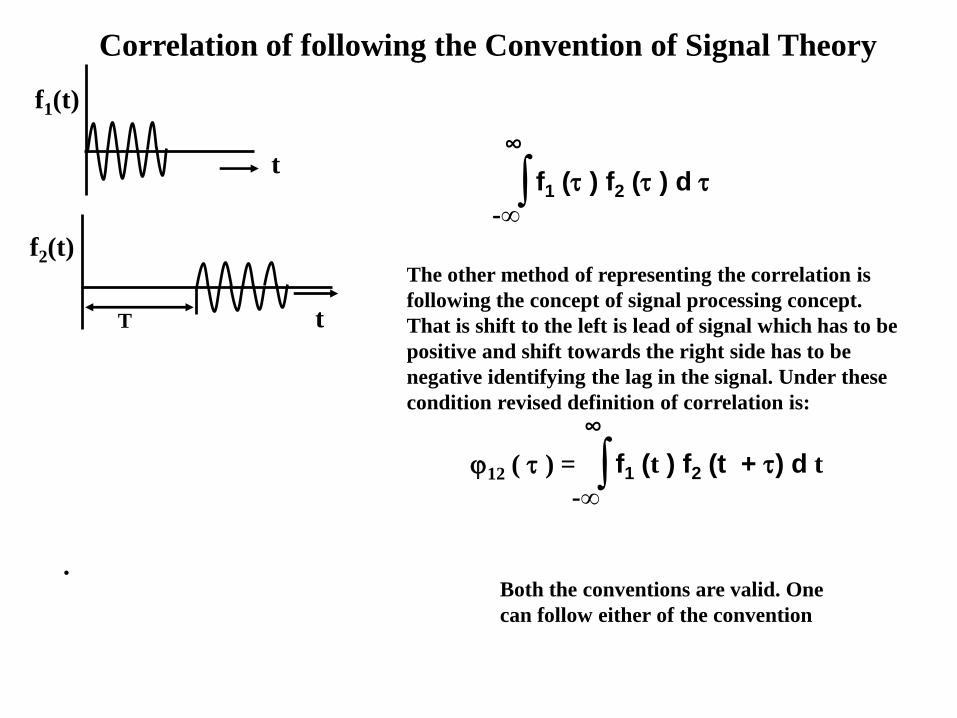
Correlation of following the Convention of Signal Theory
The other method of representing the correlation is
following the concept of signal processing concept.
That is shift to the left is lead of signal which has to be
positive and shift towards the right side has to be
negative identifying the lag in the signal. Under these
condition revised definition of correlation is:
∫-∞
∞
f1 (t ) f2 (t + ) d t12 ( ) =
. Both the conventions are valid. One
can follow either of the convention
Continuous Time
Convolution
Defining a Pulse for Zero Order Hold
If we multiply by T(t) to any signal x(t) and it is a sample and
hold circuit. Than it will hold the value of x(t) at x(0) for a
duration t +T, and it will also reduce the sample value by 1 /T.
Therefore to preserve the original sample value at t = 0, we
need to multiply the x(t) by the value T. So
t
T(t)
1/T
T
T(t) = 1/T for 0 t T
Otherwise0
We are defining the pulse as:
x /(0) = x ( 0 ) T ( t ) T
x /(1) = x ( T ) T ( t –T ) T
x /(2) = x ( 2T ) T ( t -2T ) T
T kT)-(t (kT)x (t)x-k
T
/
We can approach to x ( t ) from x/ (t) in
the limiting case T tends to zero
x /(-1) = x ( -T ) T ( t + T ) T
t
T(t) 1/T
T
T kT)-(t (kT)x (t)x-k
T
/
When T 0 than we are approaching very
close to the original signal. The physical
interpretation is that we are passing the
signal through a wide band bandwidth. So we
will get the original signal.
Representation of continuous time signal
in terms of Impulse Zero Order Hold
(t) x T kT)-(t (kT)x (t)x-k
T0 T lim
/
t
x ( t )
T 2T0 3T-T
Further as T 0 than the function x /(t)
x(t) and summation approaches to
integral
Defining a Pulse for Zero Order Hold
Originally the pulse was T (-), which is shifted towards
right side by “t” such that the centre of pulse is integer
multiple of T. That is = mT, where m is an integer
T( - )
1/T
- T
T(t - )
1/T
- T tt –T
mT
Shifted towards right side by time “t”
T() 1/T
T
T(t) = 1/T for 0 t 1/T
Otherwise0
We are defining the pulse as:
lim𝑻 →𝟎
𝜹𝑻 𝒕 → 𝜹 (𝒕)
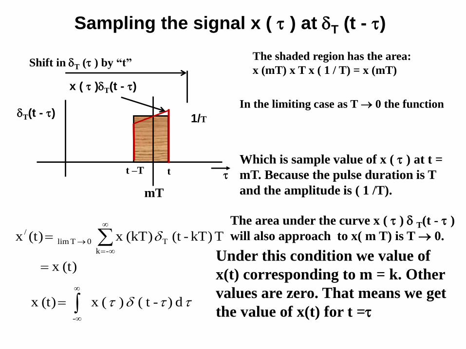
Sampling the signal x ( ) at T (t - )
T(t - )1/T
tt –T
mT
x ( )T(t - )
Shift in T ( ) by “t”
Which is sample value of x ( ) at t =
mT. Because the pulse duration is T
and the amplitude is ( 1 /T).
d ) - t ( ) (x (t)x -
Under this condition we value of
x(t) corresponding to m = k. Other
values are zero. That means we get
the value of x(t) for t =
(t) x
T kT)-(t (kT)x (t)x-k
T0 T lim
/
The shaded region has the area:
x (mT) x T x ( 1 / T) = x (mT)
The area under the curve x ( ) T(t - )
will also approach to x( m T) is T 0.
In the limiting case as T 0 the function
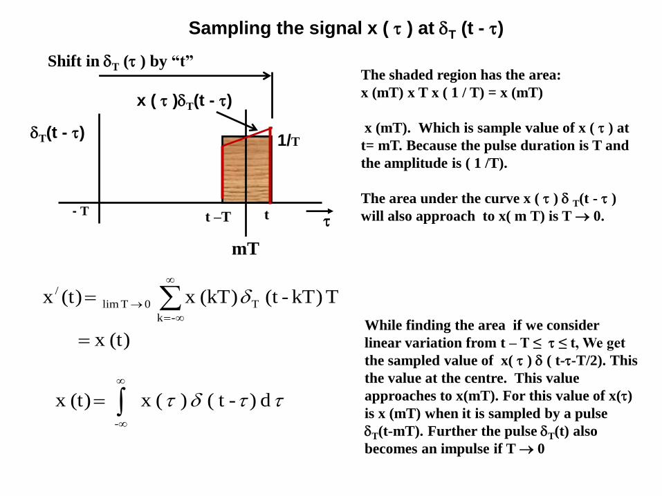
Sampling the signal x ( ) at T (t - )
T(t - )1/T
- T tt –T
mT
x ( )T(t - )
Shift in T ( ) by “t”The shaded region has the area:
x (mT) x T x ( 1 / T) = x (mT)
x (mT). Which is sample value of x ( ) at
t= mT. Because the pulse duration is T and
the amplitude is ( 1 /T).
The area under the curve x ( ) T(t - )
will also approach to x( m T) is T 0.
d ) - t ( ) (x (t)x -
While finding the area if we consider
linear variation from t – T ≤ ≤ t, We get
the sampled value of x( ) ( t--T/2). This
the value at the centre. This value
approaches to x(mT). For this value of x()
is x (mT) when it is sampled by a pulse
T(t-mT). Further the pulse T(t) also
becomes an impulse if T 0
(t) x
T kT)-(t (kT)x (t)x-k
T0 T lim
/
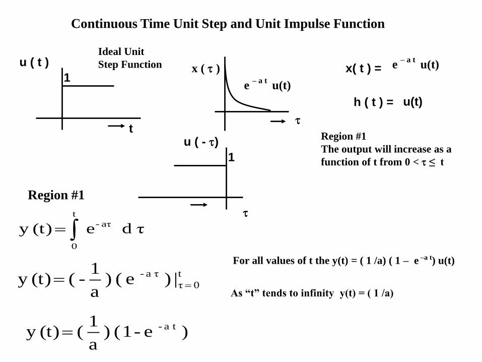
Continuous Time Unit Step and Unit Impulse Function
t
u ( t )
1
h ( t ) = u(t)
Ideal Unit
Step Function
t
0
aτ - τd e (t)y
x ( )
e – a t
u(t)
x( t ) = e – a t
u(t)
u ( - )
1
Region #1
The output will increase as a
function of t from 0 < ≤ t
As “t” tends to infinity y(t) = ( 1 /a)
Region #1
t
0 τ
τa - | ) e ( ) a
1 - ( (t)y
) e - 1 ( ) a
1 ( (t)y ta -
For all values of t the y(t) = ( 1 /a) ( 1 – e –a t) u(t)
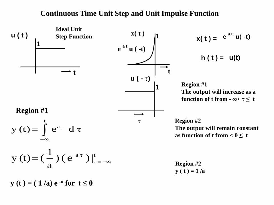
Continuous Time Unit Step and Unit Impulse Function
t
u ( t )
1
h ( t ) = u(t)
Ideal Unit
Step Function
t
aτ τd e (t)y
x( t ) = e a t
u( -t)
u ( - )
1 Region #1
The output will increase as a
function of t from - < ≤ t
Region #1
t
τ
τa | ) e ( ) a
1 ( (t)y
t
x( t ) 1
e a t
u ( -t)
y (t ) = ( 1 /a) e at for t ≤ 0
Region #2
The output will remain constant
as function of t from < 0 ≤ t
Region #2
y ( t ) = 1 /a
Sampling the signal x ( ) at T (t - )
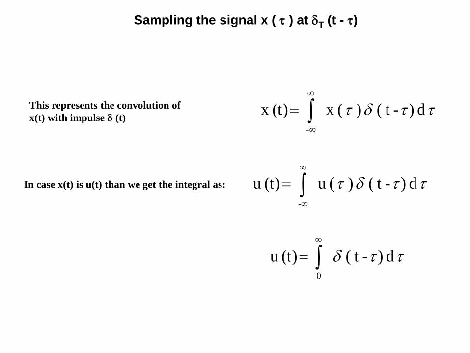
d ) - t ( ) (x (t)x -
This represents the convolution of
x(t) with impulse (t)
In case x(t) is u(t) than we get the integral as: d ) - t ( ) (u (t)u -
d ) - t ( (t)u 0

Properties of Systems

Memory and
Memoryless Systems
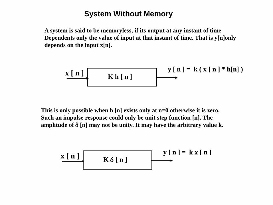
System Without Memory
A system is said to be memoryless, if its output at any instant of time
Dependents only the value of input at that instant of time. That is y[n]only
depends on the input x[n].
This is only possible when h [n] exists only at n=0 otherwise it is zero.
Such an impulse response could only be unit step function [n]. The
amplitude of [n] may not be unity. It may have the arbitrary value k.
x [ n ]K [ n ]
y [ n ] = k x [ n ]
x [ n ]K h [ n ]
y [ n ] = k ( x [ n ] * h[n] )
System Without Memory
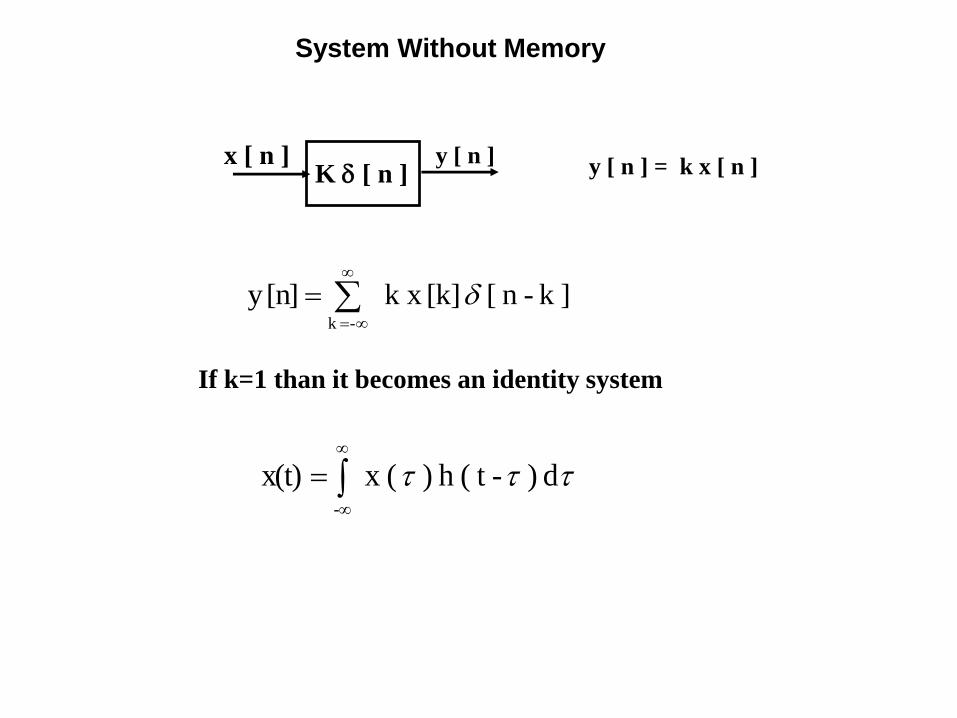
y [ n ]x [ n ]K [ n ] y [ n ] = k x [ n ]
]k -n [ [k]k x [n]y -k
If k=1 than it becomes an identity system
d ) - t (h ) (x x(t)-
System Without Memory
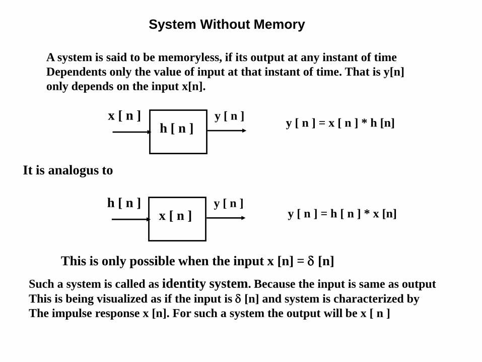
A system is said to be memoryless, if its output at any instant of time
Dependents only the value of input at that instant of time. That is y[n]
only depends on the input x[n].
Such a system is called as identity system. Because the input is same as output
This is being visualized as if the input is [n] and system is characterized by
The impulse response x [n]. For such a system the output will be x [ n ]
y [ n ]x [ n ]h [ n ] y [ n ] = x [ n ] * h [n]
This is only possible when the input x [n] = [n]
y [ n ] = h [ n ] * x [n]y [ n ]h [ n ]
x [ n ]
It is analogus to
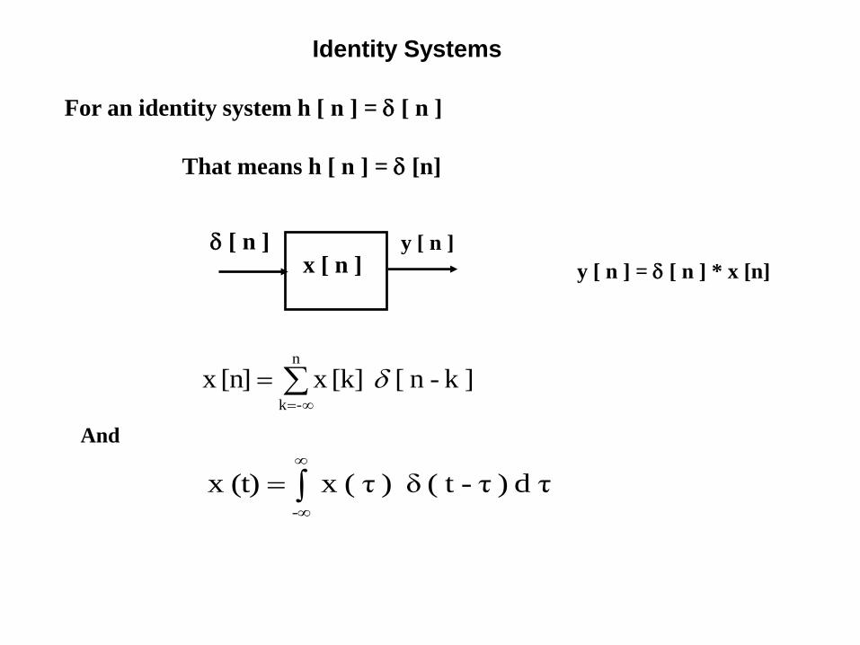
Identity Systems
That means h [ n ] = [n]
For an identity system h [ n ] = [ n ]
n
-k
]k -n [ [k]x [n]x
And
-
τd ) τ- t ( δ ) τ( x (t)x
y [ n ] = [ n ] * x [n]
y [ n ] [ n ]x [ n ]
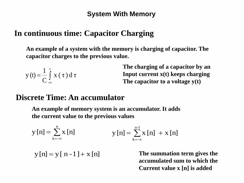
System With Memory
1-n
-k
[n] x [n]x [n]y
The summation term gives the
accumulated sum to which the
Current value x [n] is added
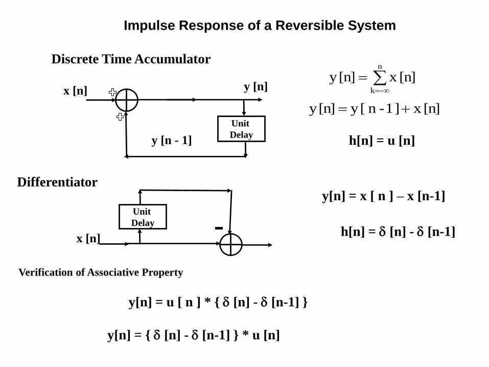
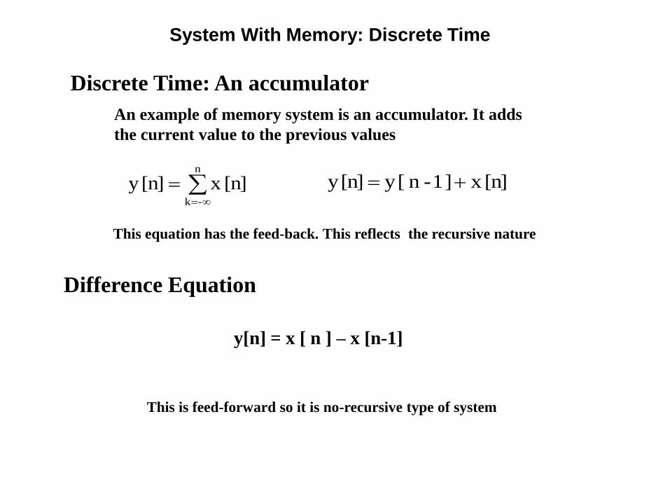
Discrete Time: An accumulator
In continuous time: Capacitor Charging
An example of a system with the memory is charging of capacitor. The
capacitor charges to the previous value.
t
-
τd ) τ( x C
1 (t)y
The charging of a capacitor by an
Input current x(t) keeps charging
The capacitor to a voltage y(t)
An example of memory system is an accumulator. It adds
the current value to the previous values
n
-k
[n]x [n]y
[n] x ] 1 -n [y [n]y
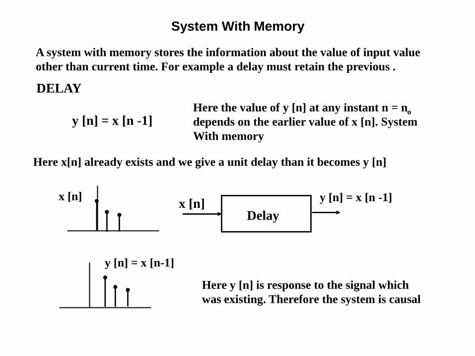
System With Memory
y [n] = x [n -1]Here the value of y [n] at any instant n = no
depends on the earlier value of x [n]. System
With memory
A system with memory stores the information about the value of input value
other than current time. For example a delay must retain the previous .
Here x[n] already exists and we give a unit delay than it becomes y [n]
y [n] = x [n -1]x [n]
Here y [n] is response to the signal which
was existing. Therefore the system is causal
y [n] = x [n-1]
DELAY
x [n]Delay
Invertibility / Inverse of Systems
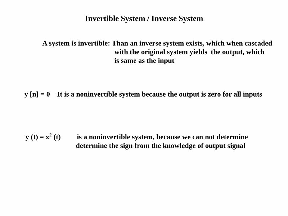
Invertible System / Inverse System
A system is invertible: Than an inverse system exists, which when cascaded
with the original system yields the output, which
is same as the input
y [n] = 0 It is a noninvertible system because the output is zero for all inputs
y (t) = x2 (t) is a noninvertible system, because we can not determine
determine the sign from the knowledge of output signal
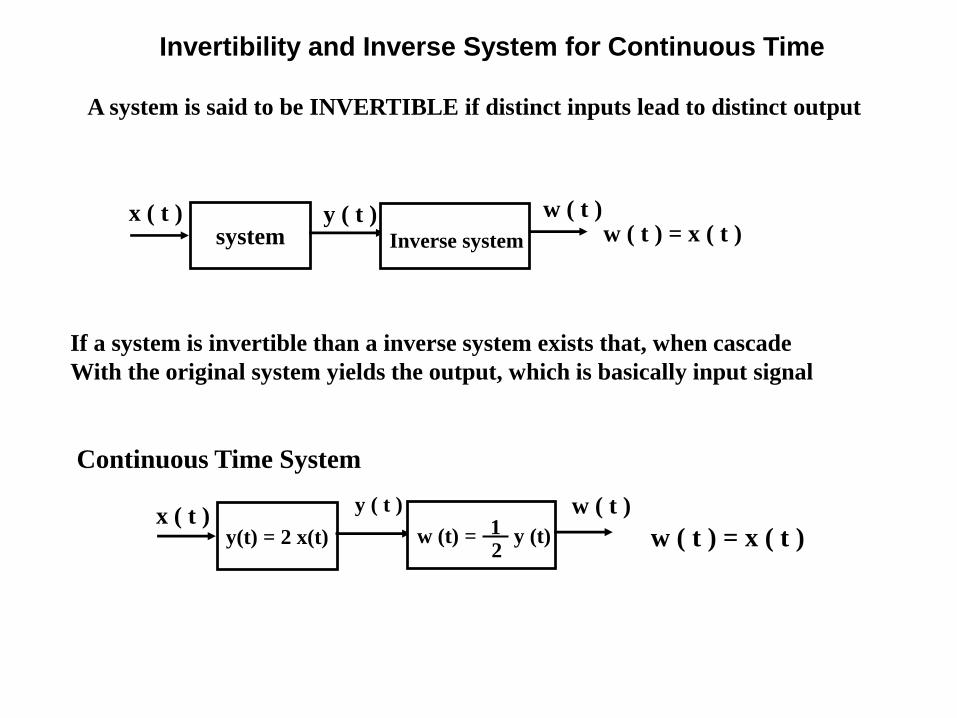
Invertibility and Inverse System for Continuous Time
A system is said to be INVERTIBLE if distinct inputs lead to distinct output
If a system is invertible than a inverse system exists that, when cascade
With the original system yields the output, which is basically input signal
Continuous Time System
y(t) = 2 x(t)x ( t )
y ( t ) w ( t )
w ( t ) = x ( t )21w (t) = y (t)
systemx ( t ) y ( t ) w ( t )
w ( t ) = x ( t )Inverse system
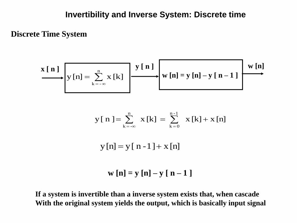
Invertibility and Inverse System: Discrete time
If a system is invertible than a inverse system exists that, when cascade
With the original system yields the output, which is basically input signal
Discrete Time System
x [ n ] y [ n ]
w [n] = y [n] – y [ n – 1 ]
w [n]
[k] x [n]y n
- k
[n] x [k] x [k] x ]n [y 1 -n
0 k
n
- k
[n] x ] 1 -n [y [n]y
w [n] = y [n] – y [ n – 1 ]

Difference Equation
Integrator
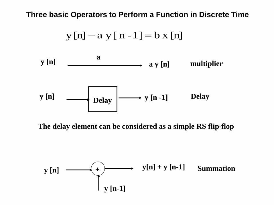
Three basic Operators to Perform a Function in Discrete Time
[n] x b ] 1 -n [y a [n]y
y [n] a y [n] a
multiplier
y [n] y [n -1] DelayDelay
+y [n]
y [n-1]
y[n] + y [n-1] Summation
The delay element can be considered as a simple RS flip-flop
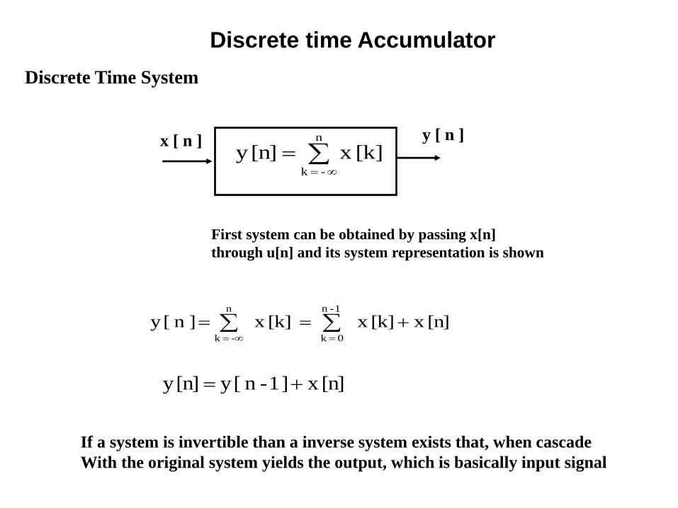
Discrete time Accumulator
If a system is invertible than a inverse system exists that, when cascade
With the original system yields the output, which is basically input signal
Discrete Time System
x [ n ] y [ n ] [k] x [n]y
n
- k
[n] x [k] x [k] x ]n [y 1 -n
0 k
n
- k
[n] x ] 1 -n [y [n]y
First system can be obtained by passing x[n]
through u[n] and its system representation is shown

System Implementation of Discrete Time Accumulator
Convolution of x[n] with h[n]
Discrete Time: An accumulator
1-n
-k
[n] x [n]x [n]y
n
-k
[n]x [n]y [n] x ] 1 -n [y [n]y
So this can be expressed as :
-k
]k -n [u [n]x [n]y
n
-k
]k -n [u [n]x [n]y
h[n] = u [n]x [n] y [n]
y [n] = x[n] * u[n]
In accumulator we add present value in the previous value. y[n] = y [n-1] + x[n]
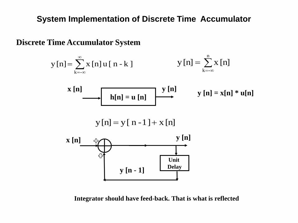
System Implementation of Discrete Time Accumulator
Discrete Time Accumulator System
n
-k
[n]x [n]y
[n] x ] 1 -n [y [n]y
-k
]k -n [u [n]x [n]y
h[n] = u [n]x [n] y [n]
y [n] = x[n] * u[n]
Unit
Delay
x [n] y [n]
y [n - 1]
Integrator should have feed-back. That is what is reflected
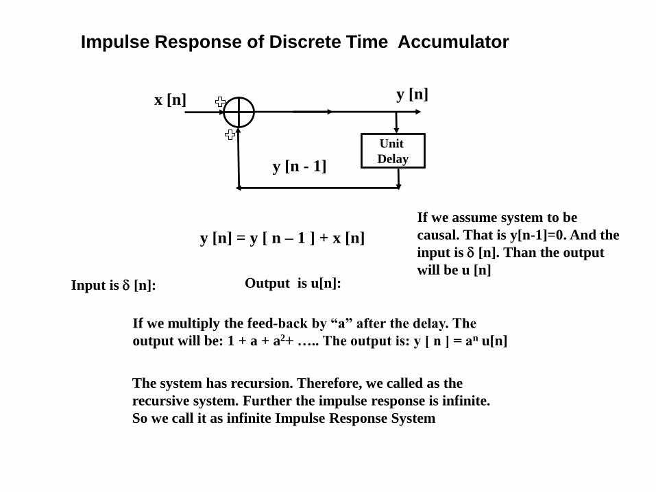
Impulse Response of Discrete Time Accumulator
Unit
Delay
x [n] y [n]
y [n - 1]
If we assume system to be
causal. That is y[n-1]=0. And the
input is [n]. Than the output
will be u [n]
y [n] = y [ n – 1 ] + x [n]
Input is [n]: Output is u[n]:
If we multiply the feed-back by “a” after the delay. The
output will be: 1 + a + a2+ ….. The output is: y [ n ] = an u[n]
The system has recursion. Therefore, we called as the
recursive system. Further the impulse response is infinite.
So we call it as infinite Impulse Response System
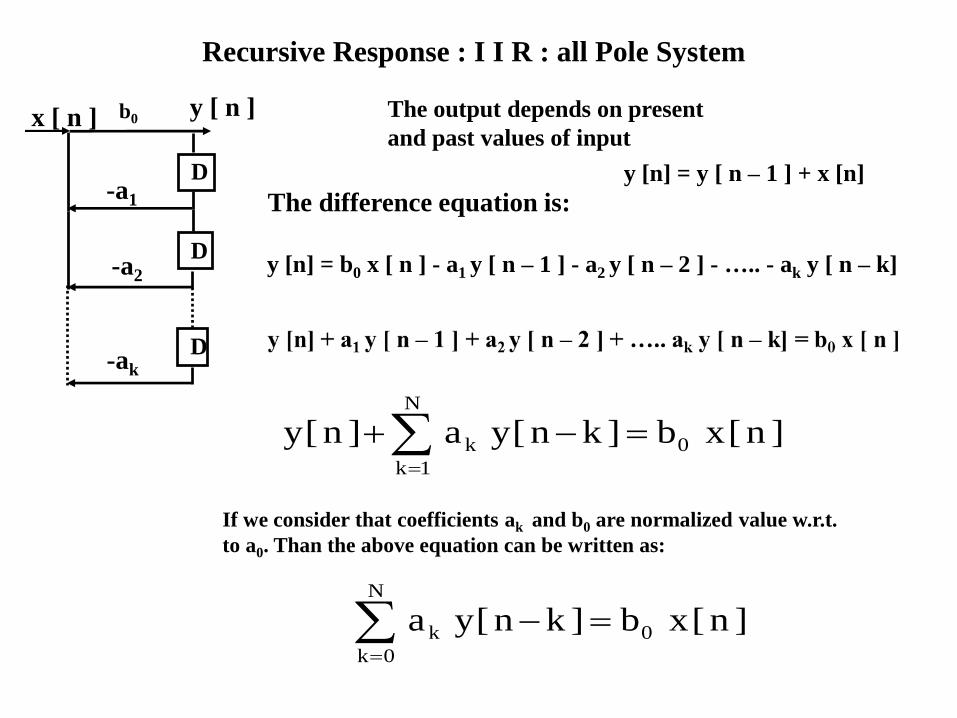
Recursive Response : I I R : all Pole System
The output depends on present
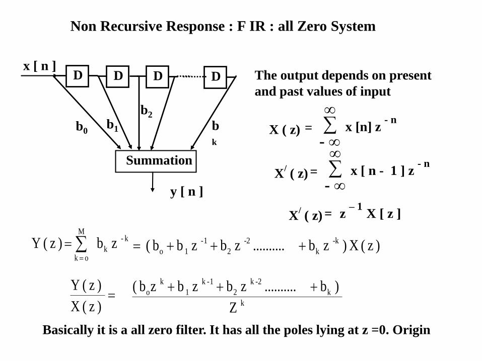
and past values of inputx [ n ] b0
D-a1
-a2
D
-ak
D
y [ n ]
The difference equation is:
y [n] = b0 x [ n ] - a1 y [ n – 1 ] - a2 y [ n – 2 ] - ….. - ak y [ n – k]
N
1k
0k ]n[xb]kn[ya]n[y
y [n] = y [ n – 1 ] + x [n]
If we consider that coefficients ak and b0 are normalized value w.r.t.
to a0. Than the above equation can be written as:
N
0k
0k ]n[xb]kn[ya
Difference Equation
Differentiator
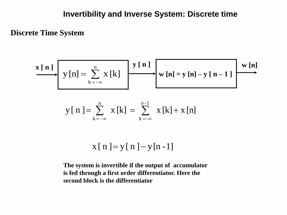
Invertibility and Inverse System: Discrete time
The system is invertible if the output of accumulator
is fed through a first order differentiator. Here the
second block is the differentiator
Discrete Time System
x [ n ] y [ n ]
w [n] = y [n] – y [ n – 1 ]
w [n]
[k] x [n]y n
- k
[n] x [k] x [k] x ]n [y 1 -n
k
n
k
1] -[n y ]n [y ]n [x
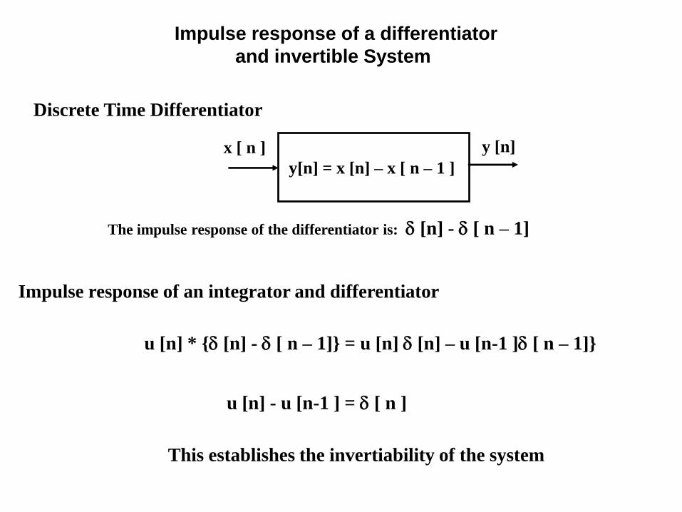
Impulse response of a differentiator
and invertible System
The impulse response of the differentiator is: [n] - [ n – 1]
Discrete Time Differentiator
x [ n ]
y[n] = x [n] – x [ n – 1 ]
y [n]
Impulse response of an integrator and differentiator
u [n] * { [n] - [ n – 1]} = u [n] [n] – u [n-1 ] [ n – 1]}
u [n] - u [n-1 ] = [ n ]
This establishes the invertiability of the system
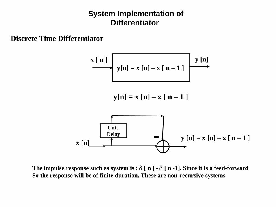
System Implementation of
Differentiator
Discrete Time Differentiator
x [ n ]
y[n] = x [n] – x [ n – 1 ]
y [n]
y[n] = x [n] – x [ n – 1 ]
y [n] = x [n] – x [ n – 1 ]
Unit
Delay
x [n]
The impulse response such as system is : [ n ] - [ n -1]. Since it is a feed-forward
So the response will be of finite duration. These are non-recursive systems
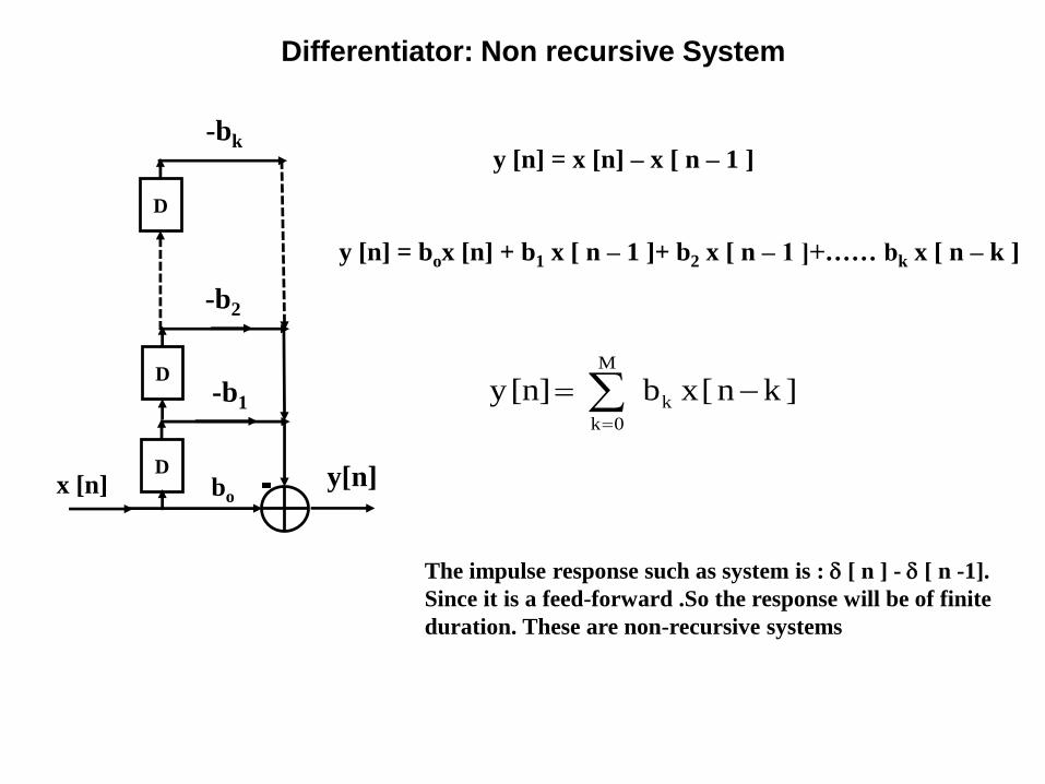
Differentiator: Non recursive System
y[n]
y [n] = x [n] – x [ n – 1 ]
Dx [n]
The impulse response such as system is : [ n ] - [ n -1].
Since it is a feed-forward .So the response will be of finite
duration. These are non-recursive systems
D
D
bo
-b1
-bk
-b2
y [n] = box [n] + b1 x [ n – 1 ]+ b2 x [ n – 1 ]+…… bk x [ n – k ]
]kn[xb [n]y k
M
0k

System With Memory: Discrete Time
Discrete Time: An accumulator
An example of memory system is an accumulator. It adds
the current value to the previous values
n
-k
[n]x [n]y [n] x ] 1 -n [y [n]y
This is feed-forward so it is no-recursive type of system
Difference Equation
y[n] = x [ n ] – x [n-1]
This equation has the feed-back. This reflects the recursive nature
Impulse Response of a Reversible System
Discrete Time Accumulator
n
-k
[n]x [n]y
[n] x ] 1 -n [y [n]y
Verification of Associative Property
Differentiatory[n] = x [ n ] – x [n-1]
Unit
Delay
x [n] y [n]
y [n - 1] h[n] = u [n]
Unit
Delay
x [n] h[n] = [n] - [n-1]
y[n] = u [ n ] * { [n] - [n-1] }
y[n] = { [n] - [n-1] } * u [n]
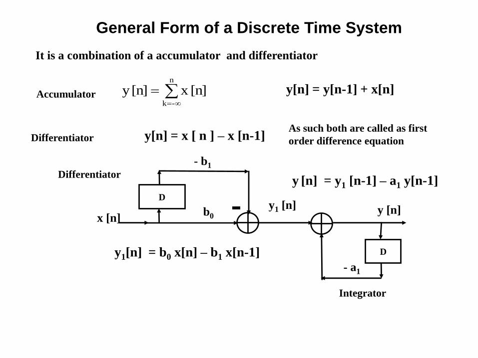
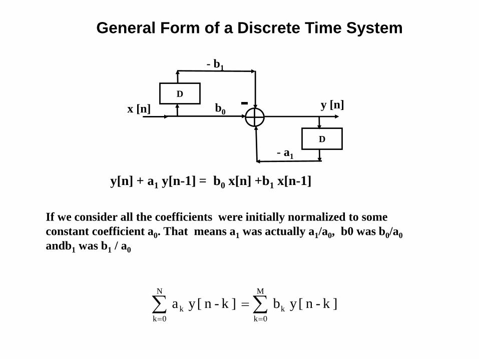
General Form of a Discrete Time System
It is a combination of a accumulator and differentiator
n
-k
[n]x [n]y y[n] = y[n-1] + x[n]Accumulator
y[n] = x [ n ] – x [n-1]DifferentiatorAs such both are called as first
order difference equation
D
x [n] b0
- b1
y [n]
D
- a1
y1[n] = b0 x[n] – b1 x[n-1]
y1 [n]
Differentiator
Integrator
y [n] = y1 [n-1] – a1 y[n-1]
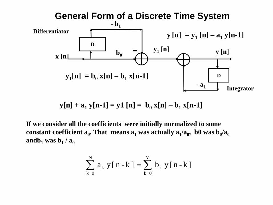
General Form of a Discrete Time System
y[n] + a1 y[n-1] = y1 [n] = b0 x[n] – b1 x[n-1]
If we consider all the coefficients were initially normalized to some
constant coefficient a0. That means a1 was actually a1/a0, b0 was b0/a0
andb1 was b1 / a0
M
0k
k
N
0k
k ]k -n [y b ]k -n [y a
D
x [n] b0
- b1
y [n]
D
- a1
y1[n] = b0 x[n] – b1 x[n-1]
y1 [n]
Differentiator
Integrator
y [n] = y1 [n] – a1 y[n-1]
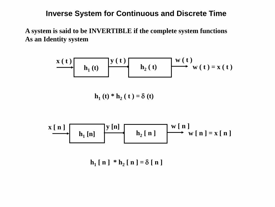
Inverse System for Continuous and Discrete Time
A system is said to be INVERTIBLE if the complete system functions
As an Identity system
h1 (t)x ( t ) y ( t ) w ( t )
w ( t ) = x ( t )h2 ( t)
h1 (t) * h2 ( t ) = (t)
h1 [n]x [ n ] y [n] w [ n ]
w [ n ] = x [ n ]h2 [ n ]
h1 [ n ] * h2 [ n ] = [ n ]
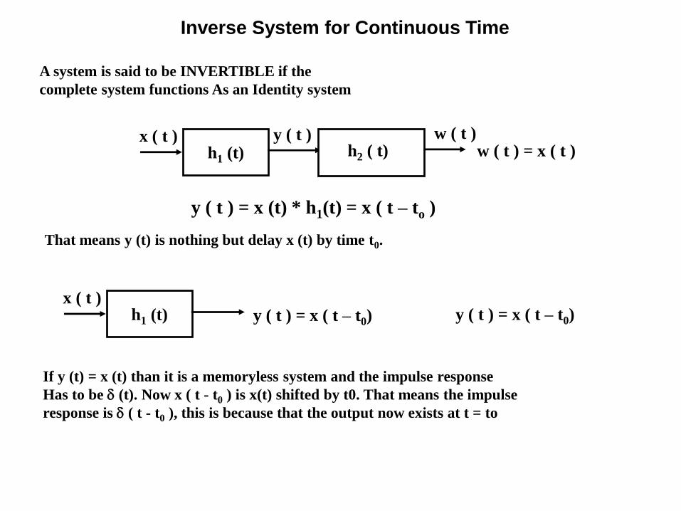
Inverse System for Continuous Time
A system is said to be INVERTIBLE if the
complete system functions As an Identity system
h1 (t)x ( t ) y ( t ) w ( t )
w ( t ) = x ( t )h2 ( t)
y ( t ) = x (t) * h1(t) = x ( t – to )
That means y (t) is nothing but delay x (t) by time t0.
h1 (t)x ( t )
y ( t ) = x ( t – t0) y ( t ) = x ( t – t0)
If y (t) = x (t) than it is a memoryless system and the impulse response
Has to be (t). Now x ( t - t0 ) is x(t) shifted by t0. That means the impulse
response is ( t - t0 ), this is because that the output now exists at t = to
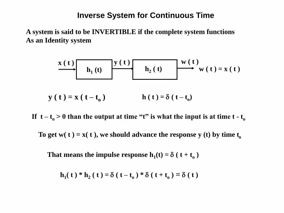
Inverse System for Continuous Time
A system is said to be INVERTIBLE if the complete system functions
As an Identity system
h1 (t)x ( t ) y ( t ) w ( t )
w ( t ) = x ( t )h2 ( t)
y ( t ) = x ( t – to ) h ( t ) = ( t – to)
If t – to > 0 than the output at time “t” is what the input is at time t - to
To get w( t ) = x( t ), we should advance the response y (t) by time to
That means the impulse response h1(t) = ( t + to )
h1( t ) * h2 ( t ) = ( t – to ) * ( t + to ) = ( t )
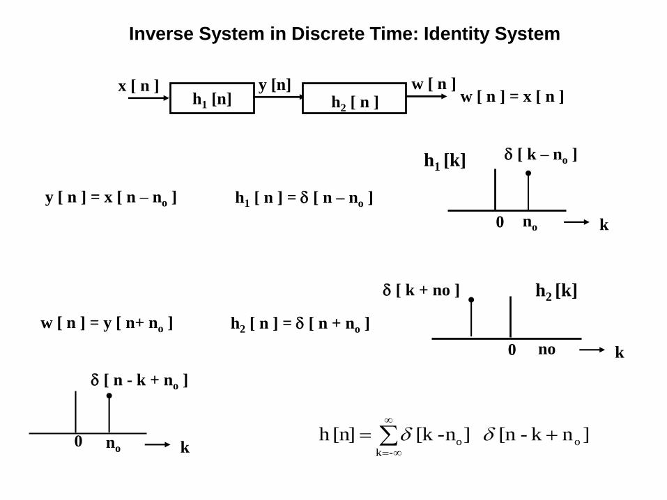
Inverse System in Discrete Time: Identity System
h1 [n]x [ n ] y [n] w [ n ]
w [ n ] = x [ n ]h2 [ n ]
y [ n ] = x [ n – no ] h1 [ n ] = [ n – no ]
w [ n ] = y [ n+ no ] h2 [ n ] = [ n + no ]
k
[ n - k + no ]
0 no
-k
oo ]n k -[n ]-n[k [n]h
k
[ k – no ]
no0
h1 [k]
k
[ k + no ]
no0
h2 [k]
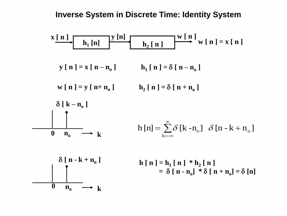
Inverse System in Discrete Time: Identity System
h1 [n]x [ n ] y [n] w [ n ]
w [ n ] = x [ n ]h2 [ n ]
h [ n ] = h1 [ n ] * h2 [ n ]
= [ n - no] * [ n + no] = [n]
y [ n ] = x [ n – no ] h1 [ n ] = [ n – no ]
w [ n ] = y [ n+ no ] h2 [ n ] = [ n + no ]
k
[ k – no ]
no0
k
[ n - k + no ]
0 no
-k
oo ]n k -[n ]-n[k [n]h

Stability of the System
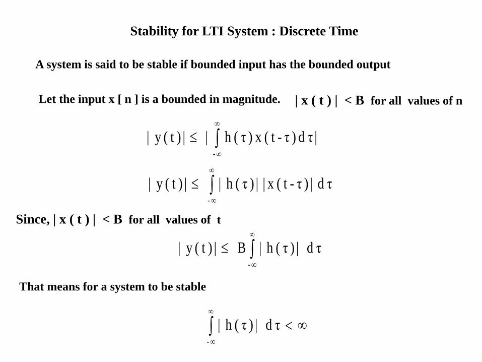
Stability for LTI System : Discrete Time
A system is said to be stable if bounded input has the bounded output
Let the input x [ n ] is a bounded in magnitude. | x ( t ) | < B for all values of n
| τd ) τ- t ( x ) τ(h | | ) t (y | -
τd | ) τ- t ( x | | ) τ(h | | ) t (y | -
Since, | x ( t ) | < B for all values of t
τd | ) τ(h | B | ) t (y | -
That means for a system to be stable
τd | ) τ(h | -
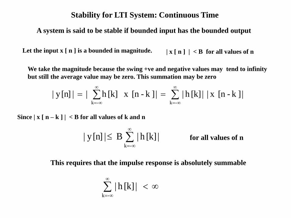
Stability for LTI System: Continuous Time
A system is said to be stable if bounded input has the bounded output
Let the input x [ n ] is a bounded in magnitude. | x [ n ] | < B for all values of n
| ]k -[n x | | [k]h | | ]k -[n x [k]h | | [n]y |-k-k
-k
| [k]h | B | [n]y |
Since | x [ n – k ] | < B for all values of k and n
This requires that the impulse response is absolutely summable
| [k]h | -k
for all values of n
We take the magnitude because the swing +ve and negative values may tend to infinity
but still the average value may be zero. This summation may be zero
Time Invariance Systems
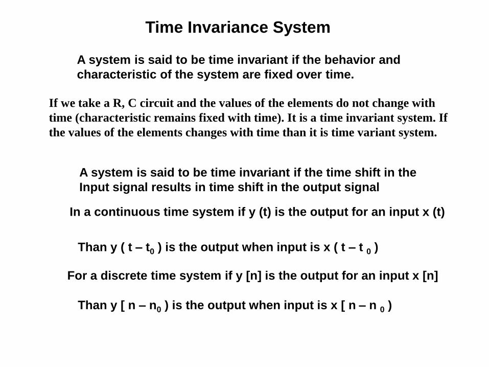
Time Invariance System
A system is said to be time invariant if the behavior and
characteristic of the system are fixed over time.
A system is said to be time invariant if the time shift in the
Input signal results in time shift in the output signal
In a continuous time system if y (t) is the output for an input x (t)
Than y ( t – t0 ) is the output when input is x ( t – t 0 )
For a discrete time system if y [n] is the output for an input x [n]
Than y [ n – n0 ) is the output when input is x [ n – n 0 )
If we take a R, C circuit and the values of the elements do not change with
time (characteristic remains fixed with time). It is a time invariant system. If
the values of the elements changes with time than it is time variant system.
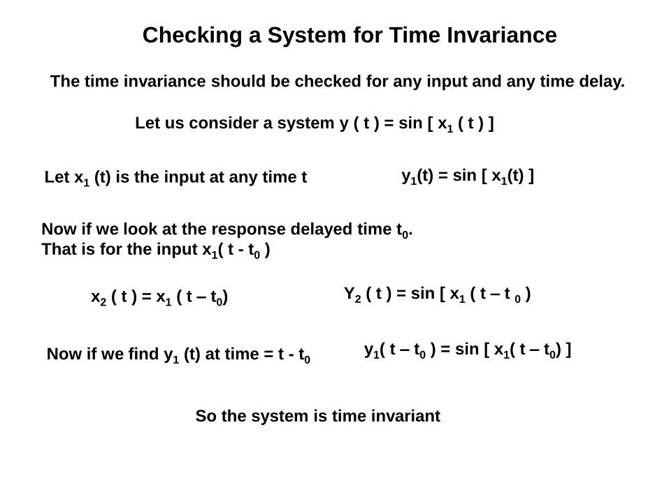
Checking a System for Time Invariance
Let us consider a system y ( t ) = sin [ x1 ( t ) ]
Let x1 (t) is the input at any time t y1(t) = sin [ x1(t) ]
Now if we look at the response delayed time t0.
That is for the input x1( t - t0 )
x2 ( t ) = x1 ( t – t0) Y2 ( t ) = sin [ x1 ( t – t 0 )
Now if we find y1 (t) at time = t - t0y1( t – t0 ) = sin [ x1( t – t0) ]
So the system is time invariant
The time invariance should be checked for any input and any time delay.
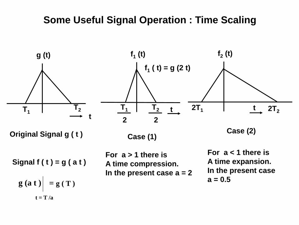
Some Useful Signal Operation : Time Scaling
t
f1 (t)
T1
2
T2
2
Case (1)
f1 ( t) = g (2 t)
For a > 1 there is
A time compression.
In the present case a = 2
t
f2 (t)
2T1 2T2
Case (2)
For a < 1 there is
A time expansion.
In the present case
a = 0.5
Original Signal g ( t )
t
g (t)
T1T2
Signal f ( t ) = g ( a t )
g (a t )
t = T /a
= g ( T )

Checking a System for Time Invariance
t
x1 (t)1
- 2 2
y ( t ) = x ( 2 t )
t
y1 (t)
-1 1
Time compression
x2 ( t ) = x1 ( t – 2 )
t
x2 (t)1
4t
y2 (t)
2
y1 ( t ) = x1 ( 2 t )
y2 ( t ) = x1 ( 2 t - 2 )
Since we have delayed x1 ( t ) by 2, we
would expect that y1 ( t ) should also be
delayed by 2 and output should be:
t
y2 (t)
1 3
Expected from
Time invariant
system
So the system is not time Invariant
Any time shift also leads time compression in output. So it is a time VARIANT SYSTEM
Causality of Systems
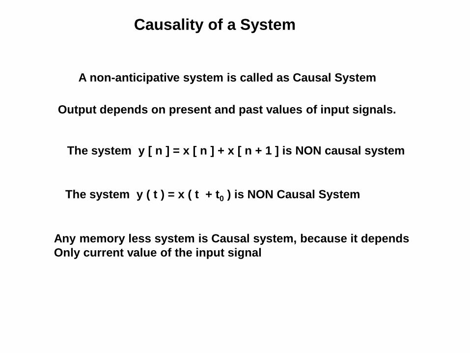
Causality of a System
A non-anticipative system is called as Causal System
Output depends on present and past values of input signals.
h(t) = 0 for t <0
A typical is charging of a capacitor. The voltage on capacitor
Depends on present past and past values of source voltage
h [n] = 0 for n <0
For a discrete time system
For a continuous system
Causality of a System for discrete System
A non-anticipative system is called as Causal System
Output depends on present and past values of input signals.
Therefore the criteria of present and past value of x[n] states that
for any shift in x[n] the h[n] must shift so:
]k -[n h [k]x [n]y -k
n
Since h [n] , for n < 0. The above expression can also be
written in alternate form by using commutative property
]k -[n h [k]x [n]y 0k
h [ n ] = 0 for n < 0
Causality of a System for Continuous Time System
A non-anticipative system is called as Causal System
Output depends on present and past values of input signals.
Therefore the criteria of present and past value of x ( t ) states that
for any shift in x (t) the h ( t ) must shift so:
Since h ( t ) , for t < 0. The above expression can also be
written in alternate form by using commutative property
h (t) = 0 for t < 0
τd ) τ- t (h ) τ( x ) t (y
t
-
τd ) τ(h ) τ- t ( x ) t (y
t
-
Causality of a System
A non-anticipative system is called as Causal System
Output depends on present and past values of input signals.
The system y [ n ] = x [ n – 1 ] is causal system
The system y ( t ) = x ( t – t0 ) is causal System
A typical is charging of a capacitor. The voltage on capacitor
Depends on present past and past values of source voltage
If a signal is defined at t = to. Than we can determine the output
at any instant later t > to.
Causality of a System
A non-anticipative system is called as Causal System
Output depends on present and past values of input signals.
The system y [ n ] = x [ n ] + x [ n + 1 ] is NON causal system
The system y ( t ) = x ( t + t0 ) is NON Causal System
Any memory less system is Causal system, because it depends
Only current value of the input signal
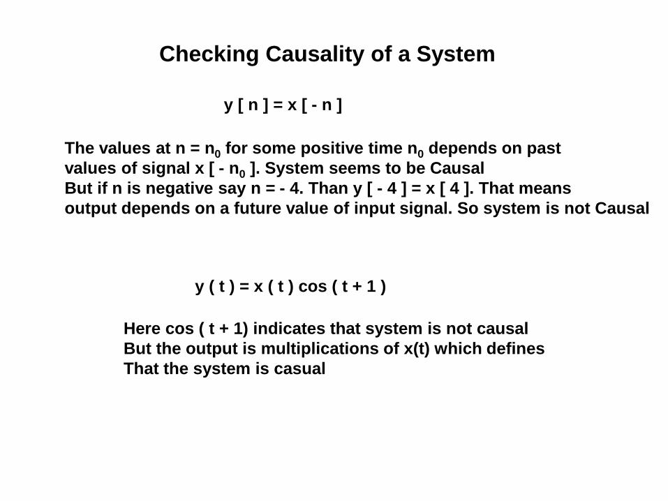
Checking Causality of a System
y [ n ] = x [ - n ]
The values at n = n0 for some positive time n0 depends on past
values of signal x [ - n0 ]. System seems to be Causal
But if n is negative say n = - 4. Than y [ - 4 ] = x [ 4 ]. That means
output depends on a future value of input signal. So system is not Causal
y ( t ) = x ( t ) cos ( t + 1 )
Here cos ( t + 1) indicates that system is not causal
But the output is multiplications of x(t) which defines
That the system is casual
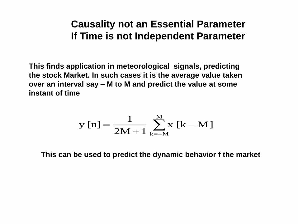
Causality not an Essential Parameter
If Time is not Independent Parameter
This finds application in meteorological signals, predicting
the stock Market. In such cases it is the average value taken
over an interval say – M to M and predict the value at some
instant of time
M
Mk
M][kx 12M
1[n]y
This can be used to predict the dynamic behavior f the market

Linear Constant
Coefficient Difference
Equation
Discrete Time
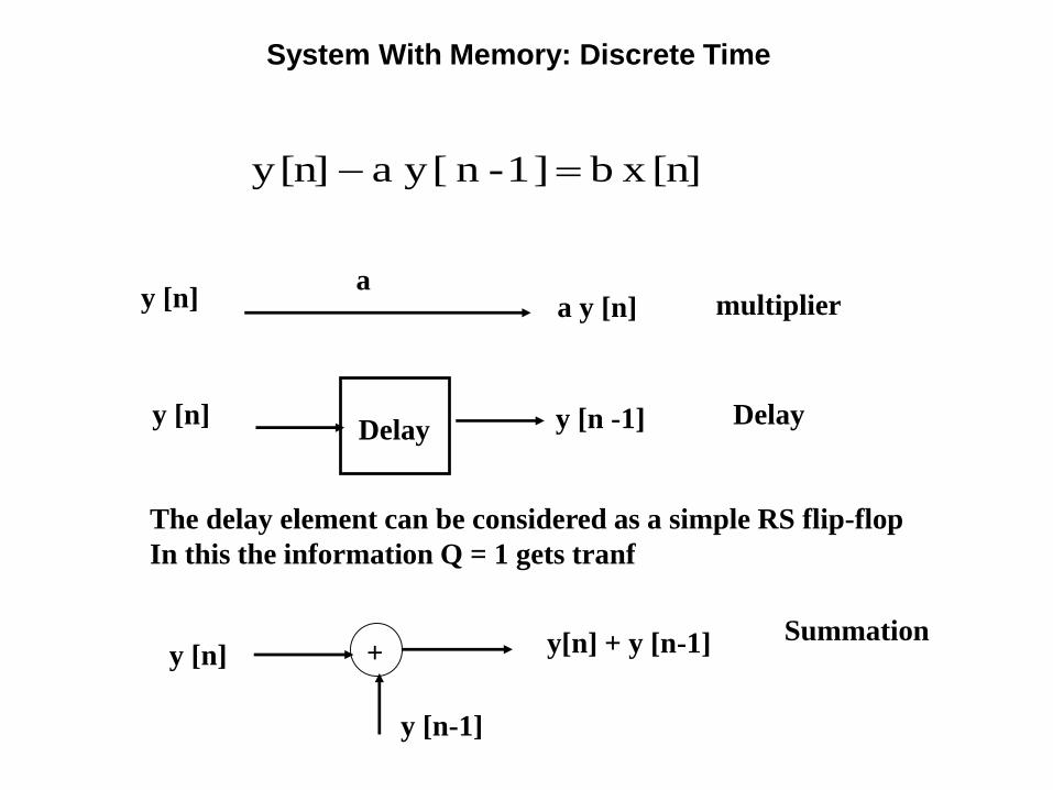
System With Memory: Discrete Time
[n] x b ] 1 -n [y a [n]y
y [n] a y [n] a
multiplier
y [n] y [n -1] DelayDelay
+y [n]
y [n-1]
y[n] + y [n-1] Summation
The delay element can be considered as a simple RS flip-flop
In this the information Q = 1 gets tranf
System With Memory: Discrete Time
Discrete Time: An accumulator
An example of memory system is an accumulator. It adds
the current value to the previous values
n
-k
[n]x [n]y [n] x ] 1 -n [y [n]y
This is feed-forward so it is no-recursive type of system
Difference Equation
y[n] = x [ n ] – x [n-1]
This equation has the feed-back. This reflects the recursive nature
General Form of a Discrete Time System
It is a combination of a accumulator and differentiator
n
-k
[n]x [n]y y[n] = y[n-1] + x[n]Accumulator
y[n] = x [ n ] – x [n-1]DifferentiatorAs such both are called as first
order difference equation
y[n] + a1 y[n-1] = b0 x[n] +b1 x[n-1]
D
x [n] b0
- b1
y1 [n]
D
- a1
y [n]
y1[n] = b0 x[n] + b1 x[n-1]
y[n] = y1[n] - a1 y[n-1]
General Form of a Discrete Time System
D
x [n] b0
- b1
y [n]
D
- a1
If we consider all the coefficients were initially normalized to some
constant coefficient a0. That means a1 was actually a1/a0, b0 was b0/a0
andb1 was b1 / a0
M
0k
k
N
0k
k ]k -n [y b ]k -n [y a
y[n] + a1 y[n-1] = b0 x[n] +b1 x[n-1]

N th Order linear constant Coefficient Difference Equation
M
0 k k
N
0 k k ]k -n [ x b ]k -n [y a
M
0 k k
N
1 k k0 ]k -n [ x b ]k -n [y a [n]y a
This equation can be expressed as:
} ]k -n [y a - ]k -n [ x b { ) a
1 ( [n]y
N
1 k k
M
0 k k
0
This equation states that for computing the present output value. We need
the information of the previous output value. From this we must realize
that we need the auxiliary conditions. That is the initial conditions.
To compute y [n] we need the information on y [n-1], ……..y [ n – N]
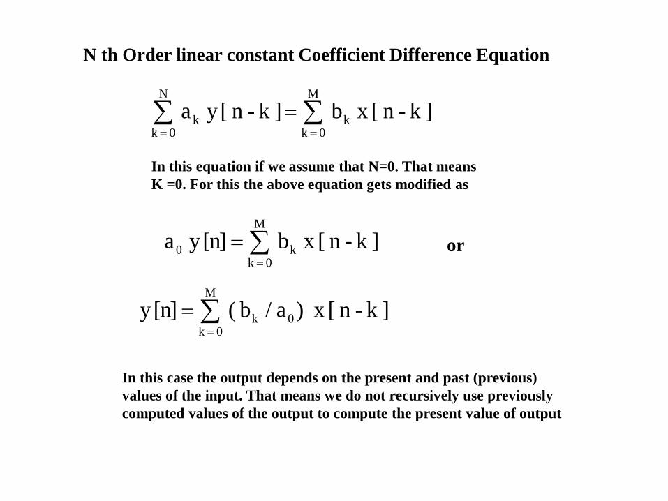
N th Order linear constant Coefficient Difference Equation
M
0 k k
N
0 k k ]k -n [ x b ]k -n [y a
In this equation if we assume that N=0. That means
K =0. For this the above equation gets modified as
M
0 k 0k ]k -n [ x )a / b ( [n]y
M
0 k k0 ]k -n [ x b [n]y a or
In this case the output depends on the present and past (previous)
values of the input. That means we do not recursively use previously
computed values of the output to compute the present value of output
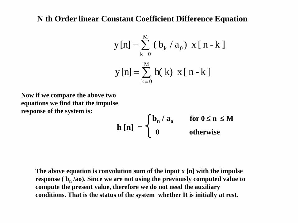
N th Order linear Constant Coefficient Difference Equation
M
0 k 0k ]k -n [ x )a / b ( [n]y
M
0 k
]k -n [ x k) h( [n]y
Now if we compare the above two
equations we find that the impulse
response of the system is:
h [n] = bn / ao for 0 n M
0 otherwise
The above equation is convolution sum of the input x [n] with the impulse
response ( bn /ao). Since we are not using the previously computed value to
compute the present value, therefore we do not need the auxiliary
conditions. That is the status of the system whether It is initially at rest.
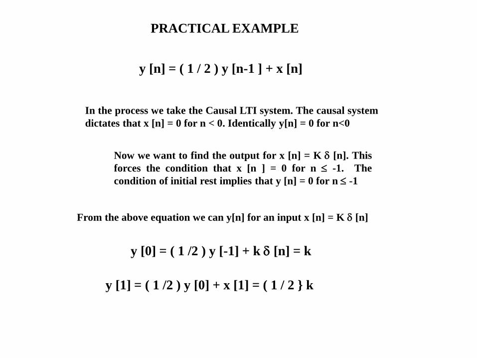
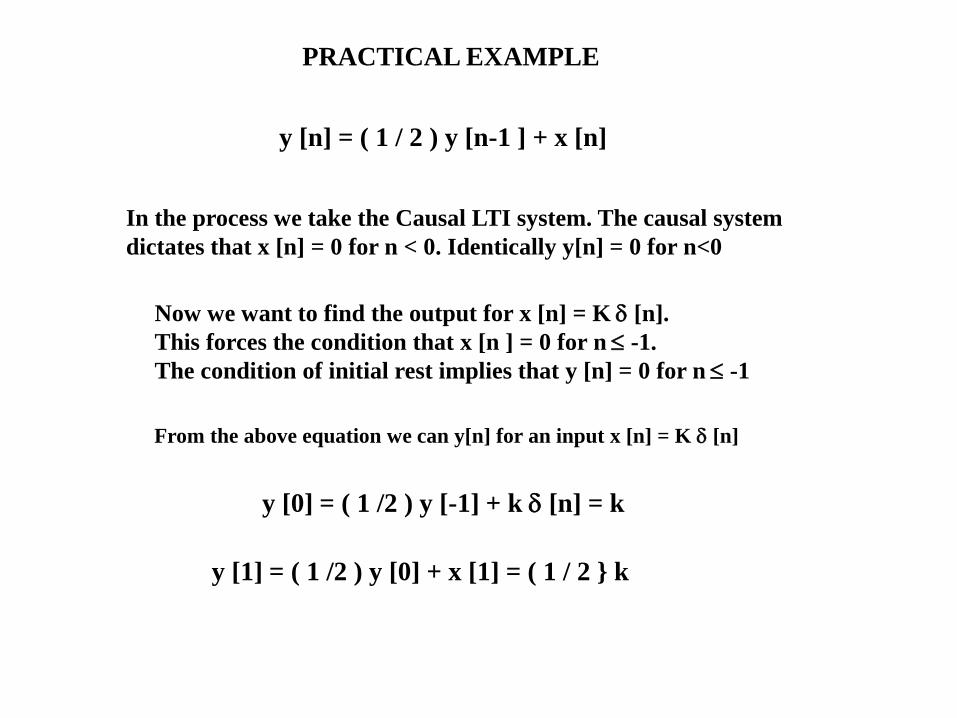
PRACTICAL EXAMPLE
y [n] = ( 1 / 2 ) y [n-1 ] + x [n]
Now we want to find the output for x [n] = K [n]. This
forces the condition that x [n ] = 0 for n -1. The
condition of initial rest implies that y [n] = 0 for n -1
In the process we take the Causal LTI system. The causal system
dictates that x [n] = 0 for n < 0. Identically y[n] = 0 for n<0
From the above equation we can y[n] for an input x [n] = K [n]
y [0] = ( 1 /2 ) y [-1] + k [n] = k
y [1] = ( 1 /2 ) y [0] + x [1] = ( 1 / 2 } k
PRACTICAL EXAMPLE
y [n] = ( 1 / 2 ) y [n-1 ] + x [n]
Now we want to find the output for x [n] = K [n].
This forces the condition that x [n ] = 0 for n -1.
The condition of initial rest implies that y [n] = 0 for n -1
In the process we take the Causal LTI system. The causal system
dictates that x [n] = 0 for n < 0. Identically y[n] = 0 for n<0
From the above equation we can y[n] for an input x [n] = K [n]
y [0] = ( 1 /2 ) y [-1] + k [n] = k
y [1] = ( 1 /2 ) y [0] + x [1] = ( 1 / 2 } k
PRACTICAL EXAMPLE
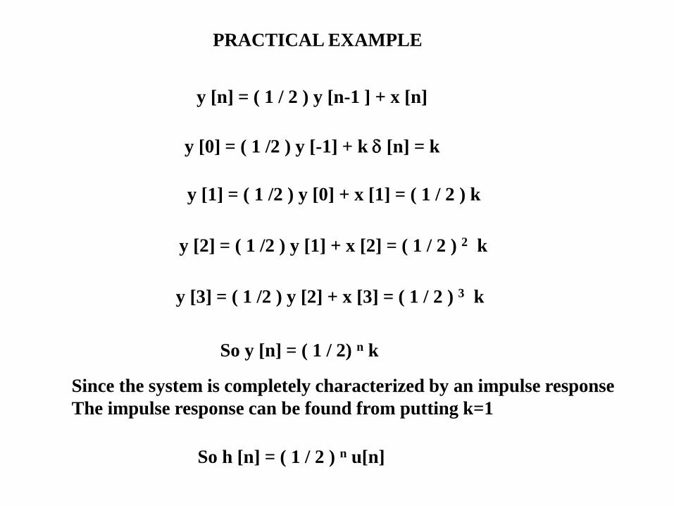
y [n] = ( 1 / 2 ) y [n-1 ] + x [n]
y [0] = ( 1 /2 ) y [-1] + k [n] = k
y [1] = ( 1 /2 ) y [0] + x [1] = ( 1 / 2 ) k
y [2] = ( 1 /2 ) y [1] + x [2] = ( 1 / 2 ) 2 k
y [3] = ( 1 /2 ) y [2] + x [3] = ( 1 / 2 ) 3 k
So y [n] = ( 1 / 2) n k
Since the system is completely characterized by an impulse response
The impulse response can be found from putting k=1
So h [n] = ( 1 / 2 ) n u[n]
Linear Constant
Coefficient Difference
Equation
Discrete Time

Miscellaneous Slides
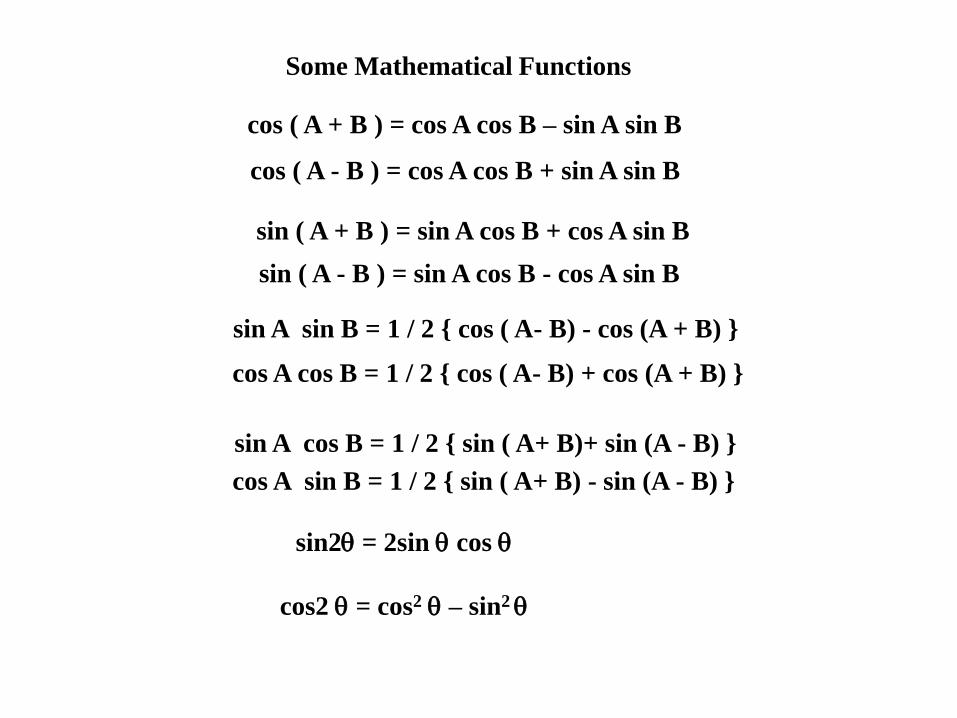
Some Mathematical Functions
cos ( A + B ) = cos A cos B – sin A sin B
cos ( A - B ) = cos A cos B + sin A sin B
sin ( A + B ) = sin A cos B + cos A sin B
sin ( A - B ) = sin A cos B - cos A sin B
sin A sin B = 1 / 2 { cos ( A- B) - cos (A + B) }
cos A cos B = 1 / 2 { cos ( A- B) + cos (A + B) }
sin A cos B = 1 / 2 { sin ( A+ B)+ sin (A - B) }
cos A sin B = 1 / 2 { sin ( A+ B) - sin (A - B) }
sin2 = 2sin cos
cos2 = cos2 – sin2
Linear Constant Coefficient Difference Equation
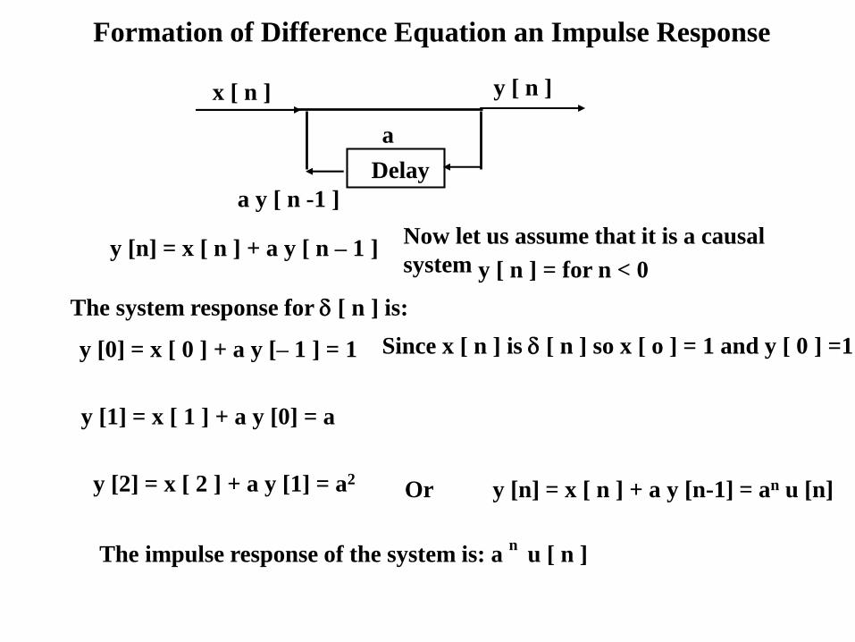
Formation of Difference Equation an Impulse Response
Delay
x [ n ] y [ n ]
a y [ n -1 ]
a
y [n] = x [ n ] + a y [ n – 1 ]Now let us assume that it is a causal
system y [ n ] = for n < 0
The system response for [ n ] is:
y [0] = x [ 0 ] + a y [– 1 ] = 1 Since x [ n ] is [ n ] so x [ o ] = 1 and y [ 0 ] =1
y [1] = x [ 1 ] + a y [0] = a
y [2] = x [ 2 ] + a y [1] = a2Or y [n] = x [ n ] + a y [n-1] = an u [n]
The impulse response of the system is: a n
u [ n ]
The output depends on present
and past values of input
Summation
x [ n ]
y [ n ]
b
k
D D D D
b0b1
b2
X ( z) = ∑- ∞
∞x [n] z
- n
X/( z) = ∑
- ∞
∞x [ n - 1 ] z
- n
X/( z) = z
– 1X [ z ]
z b ) z ( Y k -
k
M
o k
) z ( X ) z b .......... z b z b b ( -k
k
-2
2
1 -
1 o
) z ( X
) z ( Y
k
k
2-k
2
1 -k
1
k
o
Z
) b .......... z b z b zb (
Basically it is a all zero filter. It has all the poles lying at z =0. Origin
Non Recursive Response : F IR : all Zero System
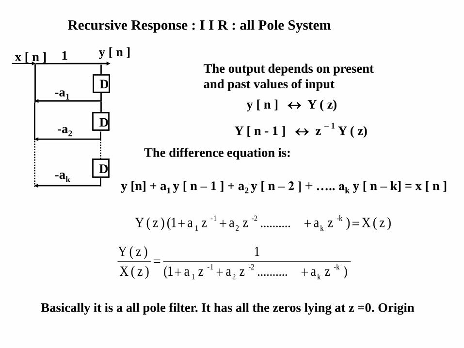
Recursive Response : I I R : all Pole System
The output depends on present
and past values of input
y [ n ] Y ( z)
) z ( X ) z a .......... z a z a (1 ) z ( Y -k
k
-2
2
1 -
1
Basically it is a all pole filter. It has all the zeros lying at z =0. Origin
Y [ n - 1 ] z – 1
Y ( z)
x [ n ] 1
D-a1
-a2
D
-akD
y [ n ]
The difference equation is:
y [n] + a1 y [ n – 1 ] + a2 y [ n – 2 ] + ….. ak y [ n – k] = x [ n ]
) z a .......... z a z a (1
1
) z ( X
) z ( Y
k-
k
2-
2
1 -
1
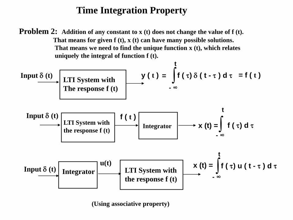
Time Integration Property
Problem 2: Addition of any constant to x (t) does not change the value of f (t).
That means for given f (t), x (t) can have many possible solutions.
That means we need to find the unique function x (t), which relates
uniquely the integral of function f (t).
LTI System with
The response f (t)
Input (t) ∫- ∞
t
y ( t ) = f ( ) ( t - ) d = f ( t )
LTI System with
the response f (t)
Input (t) f ( t )
∫- ∞
t
x (t) = f ( ) d Integrator
LTI System with
the response f (t)
Input (t) ∫- ∞
t
x (t) = f ( ) u ( t - ) d Integrator
u(t)
(Using associative property)