controlling chaos and bifurcation of subsynchronous resonance in … · · 2012-06-22controlling...

Nonlinear Analysis: Modelling and Control, 2002, Vol. 7, No. 2, 15–36

15

Controlling Chaos and Bifurcation of Subsynchronous Resonance in Power System

A.M. Harb, M.S. Widyan Department of Electrical Engineering

Jordan University of Science and Technology P.O.Box 3030, Ibid, Jordan

[email protected]

Received: date 26.06.2002 Accepted: date 13.11.2002

Abstract. Linear and nonlinear state feedback controllers are proposed to control the bifurcation of a new phenomenon in power system, this phenomenon of electro-mechanical interaction between the series resonant circuits and torsional mechanical frequencies of the turbine generator sections, which known as Subsynchronous Resonance (SSR). The first system of the IEEE second benchmark model is considered. The dynamics of the two axes damper windings, Automatic Voltage Regulator (AVR) and Power System Stabilizer (PSS) are included. The linear controller gives better initial disturbance response than that of the nonlinear, but in a small narrow region of compensation factors. The nonlinear controller not only can be easily implemented, but also it stabilizes the operating point for all values of the bifurcation parameter.

Keywords: subsynchronous resonance, power system, control of chaos.

1 Introduction

The phenomenon of SSR has been studied very extensively since 1970 when a major transmission network in the USA experienced shaft failure to its T-G unit with series compensation in the 500KV lines. This has now gone into technical literature as a classical problem and known as Project Navajo. However, this phenomenon had been known to exist for a few years according to many experts who predicted such a phenomenon in series-compensated lines connected to T-G units [1]. In fact, series compensation has been considered as a powerful alternative based on economic and technical considerations for increasing

A.M. Harb, M.S. Widyan

16

effectively the power transfer capability and improving the stability of extra high voltage systems.

In the last few years, power system dynamics have been studied from nonlinear dynamics point of view using bifurcation theory. In fact, power system has rich bifurcation phenomena. Particularly, when the consumer demand for reactive power reaches its peaks, the dynamics of an electric power network may move to its stability margin, leading to oscillations and bifurcations.

SSR is a phenomenon in power system in which bifurcation theory can be applied. The most commonly encountered bifurcation is the dynamic bifurcation “Hopf bifurcation” in which a complex conjugate pair of eigenvalues of the linearized model around the operating condition transversally crosses the imaginary axis of the complex plane. The birth of limit cycle from an equilibrium point gives rise to oscillations, which may undergo complicated bifurcations such as period multiplication, cyclic folds or crises. Zhu et al. [2] used the Hopf bifurcation theorem, in which the dynamics of the AVR and damper windings are neglected, to study a SMIB power system experienced SSR, a prediction of supercritical Hopf bifurcation is investigated. The bifurcation analysis is used by Nayfeh et al. [3] to investigate the complex dynamics of a heavily loaded SMIB power system modeling the characteristics of the BOARDMAN generator with respect to the rest of the North-Western American Power System. In their study, the dynamic effects of d- and q-axes damper windings are included while that of the AVR is neglected. The results show that, as the compensation factor increases the operating point loses stability via supercritical Hopf bifurcation. On further increase of the compensation factor the system route to chaos via torus breakdown. Also it is concluded that the effect of the damper windings on that system is to destabilize the system by reducing the compensation level at which SSR occurs. The effect of electrical machine saturation on SSR is also studied by Harb et al. [4]; they concluded that, the generator saturation slightly shrinks the positively damped region by shifting the Hopf bifurcation point to smaller compensation level. It also slightly shifts the secondary Hopf bifurcation and blue sky catastrophe to smaller compensation level.

Bifurcation control deals with modification of bifurcation characteristics of a parameterized nonlinear system by a designed control input. Typical

Controlling Chaos and Bifurcation

17

bifurcation control objectives include delaying the onset of an inherent bifurcation [5] and [6], introducing a new bifurcation at a preferable parameter value [7] and [8], changing the parameter value of an existing bifurcation point [9] and [10], modifying the shape or type of a bifurcation chain [6], stabilizing a bifurcated solution or branch [11] and [12], monitoring the multiplicity [13], amplitude [14], and/or frequency of some limit cycles emerging from bifurcation [15] and optimizing the system performance near a bifurcation point [16].

Bifurcation control with various objectives have been implemented in experimental systems or tested by using numerical simulations in a great number of engineering, biological, and physicochemical systems; examples can be named in chemical engineering [17] and [18], mechanical engineering [19]–[21], electrical engineering [22]–[28], biology [29], physics and chemistry [30]–[32] and meteorology [33]. Bifurcation control is not only important in its own right, but also suggests a viable and effective strategy for chaos control, this because the bifurcation and chaos are usually twins.

It is now known that bifurcation properties of a system can be modified via various feedback control methods. Representative approaches employ linear or nonlinear state-feedback controls [8], [11], [34] and [35], apply a washout filter-aided dynamic feedback controller [35], and use harmonic balance approximations [10].

The aims of the paper are to use linear and nonlinear controllers to control bifurcation and chaos of SSR for the IEEE second benchmark model, and to compare between these two types of controllers.

The paper is organized as follows: In section 2, a description of the considered system is given. Section 3 gives the mathematical model of the open loop system. Section 4 discussed the used linear and nonlinear state feedback controllers. Numerical simulation results for both open and closed loop systems are given in section 5, and finally some conclusions are withdrawn in section 6.

2 System Description

After Harb & Widyan [36], we considered the first system of the IEEE second benchmark models of subsynchronous resonance. As shown in fig. 1, it is a


18

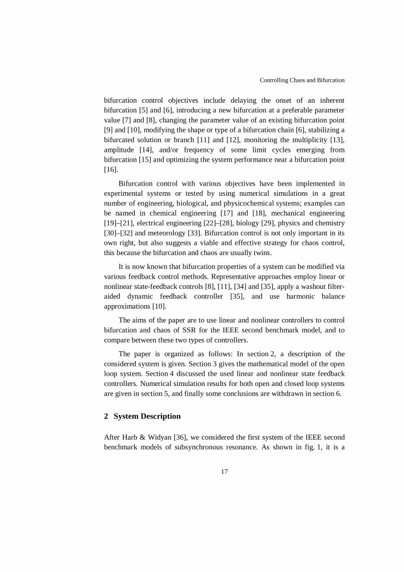
SMIB power system with two transmission lines, one of them is compensated by a series capacitor.

Fig. 1. Power system under study (System 1, IEEE Second Benchmark Model of SSR)

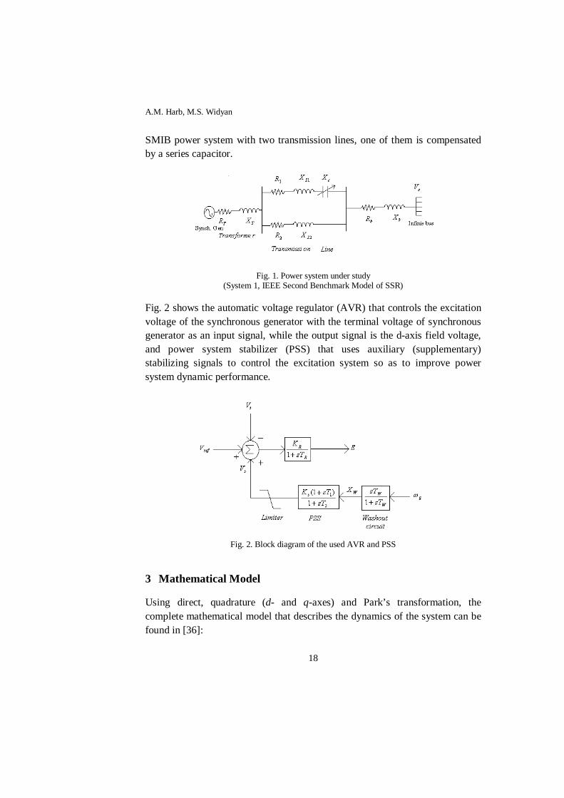
Fig. 2 shows the automatic voltage regulator (AVR) that controls the excitation voltage of the synchronous generator with the terminal voltage of synchronous generator as an input signal, while the output signal is the d-axis field voltage, and power system stabilizer (PSS) that uses auxiliary (supplementary) stabilizing signals to control the excitation system so as to improve power system dynamic performance.

Fig. 2. Block diagram of the used AVR and PSS

3 Mathematical Model

Using direct, quadrature (d- and q-axes) and Park’s transformation, the complete mathematical model that describes the dynamics of the system can be found in [36]:


19

a) Synchronous Generator:

fdfdoafd

fdo

kdfkd

dafd

fdffd irE

Xr

dtdiX

dtdiX

dtdi

X ωω −=+− , (1)

dtdiX

dtdiXkXXX

dtdi

X kdakd

dbLTd

fdafd ++++− )( 1

daTbogoo irkRRRV )(sin 1 ++++= ωδω (2)

,)( 1 cdokqakqgoqqgLbTo viXiXkXXX ωωωωω ++++++−

where 2

1212

21

22

22

)()( LLL

L

XXXRR

XRk

µ−+++

+

= ,

kdkdokd

kkdd

akdfd

fkd irdt

diXdtdiX

dtdi

X ω−=+− , (3)

dtdi

Xdtdi

XkXXX kqakq

qbLTq ++++− )( 1

ddgLbTofdafdgogoo iXkXXXiXV )(cos 1 ωωωωδω ++++−= (4)

,)( 1 cqoqabTokdakdgo virkRRRiX ωωωω +++++−

irdt

diX

dtdi

X kqokq

kkqq

akq ω−=+− . (5)

b) Transmission Line:

With 1Lc XX µ= ,

cqodLocd vikX

dtdv

ωµω −= 1 , (6)

cdoqLocq vikX

dtdv

ωµω −= 1 . (7)

c) Mechanical System:

011

ωωωδ

−= odtd , (8)

ggg KKDDdt

dM δδωω

1111111

1 +−−= , (9)


20

ogog

dtd

ωωωδ

−= , (10)

,222111 δδδδ

ω

ω

gggggg

ggdkqakqdqqqkdakd

dqdfdqafdgmg

g

KKKKDiiXiiXiiX

iiXiiXDTdt

dM

+−−+

−+−−

+−+=

(11)

oodtd

ωωωδ

−= 22 , (12)

3232232222222

2 δδδδωω KKKKDDdt

dM ggg +−−+−= , (13)

oodtd

ωωωδ

−= 33 , (14)

3232233333

3 δδωω KKDDdt

dM −+−= . (15)

d) Automatic Voltage Regulator (AVR) and Power System Stabilizer (PSS) Mathematical Model

The mathematical model of AVR and PSS (fig. 2) is given by the following equations:

Wg

WW

W Xdt

dT

dtdXT −=−

ω

, (16)

sWsW

sS VXK

dtdXKT

dtdVT −=− 12 , (17)

EVKVKVKdtdET tRsRrefRR −−+= . (18)

With 22qdt VVV += , neglecting stator transients yields:

qqdad iXirV +−= ,

fdafdddqaq iXiXirV +−−= .

Consequently,

tV 22 )()( fdafdddqaqqda iXiXiriXir +−−++−= . (19)


21

Hence, the system can be written in state space representation in the form:

);( µxFdtdx

= , (20)

whereµ is the bifurcation parameter, representing the compensation factor ( 1/ Lc XX ) of the power system. In all cases, the system has more than one equilibrium solution; the selected one is the equilibrium, which represent the operating point resulting in a heavily loaded generator with 9.0=Pe ,

43.0=eQ and 138.1=tV pu.

Equations (1)–(19) give a complete description to the dynamics of the SMIB power system with two transmission lines one of them is compensated by a series capacitor. The state variables are fdix =1 , dix =2 , kdix =3 , qix =4 ,

kqix =5 , cdvx =6 , cqvx =7 , 18 δ=x , 19 ω=x , gx δ=10 , gx ω=11 , 212 δ=x ,

213 ω=x , 314 δ=x , 315 ω=x , WXx =16 , sVx =17 and Ex =18 . All parameters are given in the Appendix.

4 Linear and Nonlinear State Feedback Controller

4.1 Linear State Feedback Controller. It is based on the linearized version around the operating point of the nonlinear dynamical system. The control is achieved by feeding back the state variables through a regulator with constant gains. Consider the following linearized version of a nonlinear system in the state-variable form [37]:

BuAxdtdx

+= , (21)

where A is an nn× constant matrix and B is an mn× constant matrix, here m is the number of the system inputs, given by

xxA

∂

∂=

.

, uxB

∂

∂=

.

(22)

evaluated at the operating point.

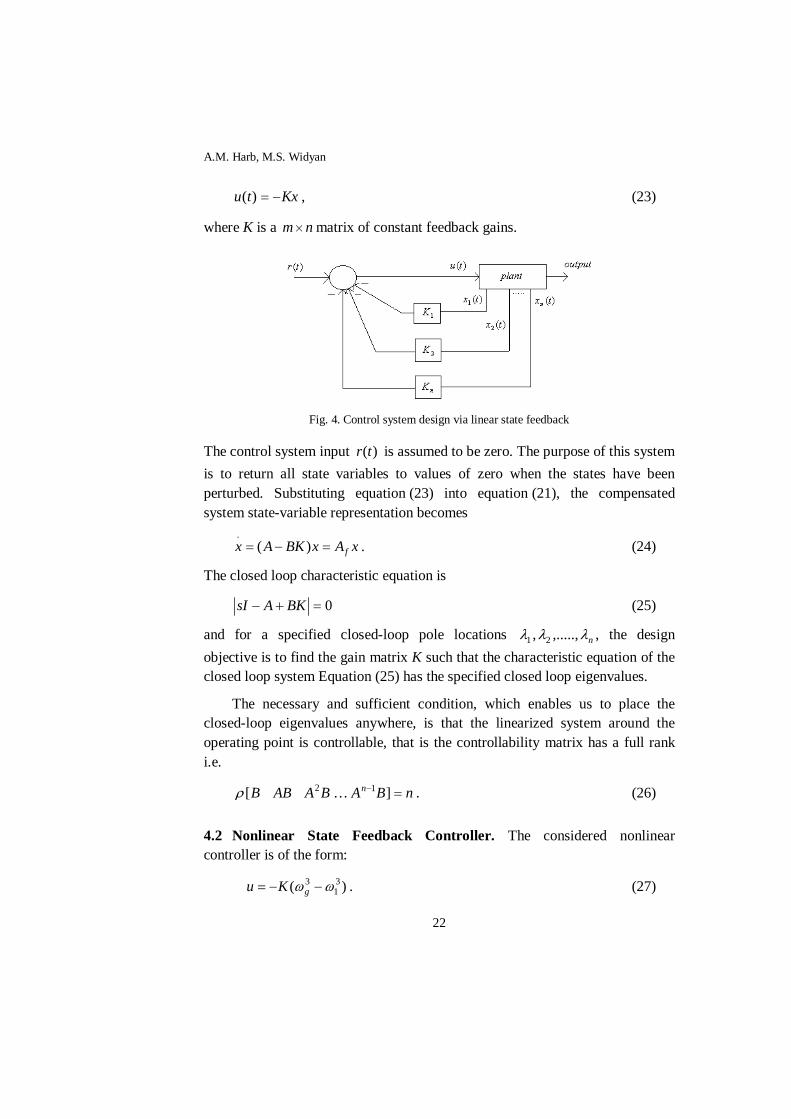
Now consider the block diagram of the system shown in fig. 4 with the following state feedback control


22

Kxtu −=)( , (23)

where K is a nm× matrix of constant feedback gains.

Fig. 4. Control system design via linear state feedback

The control system input )(tr is assumed to be zero. The purpose of this system is to return all state variables to values of zero when the states have been perturbed. Substituting equation (23) into equation (21), the compensated system state-variable representation becomes

xAxBKAx f=−= )(.

. (24)

The closed loop characteristic equation is

0=+− BKAsI (25)

and for a specified closed-loop pole locations nλλλ ,.....,, 21 , the design objective is to find the gain matrix K such that the characteristic equation of the closed loop system Equation (25) has the specified closed loop eigenvalues.

The necessary and sufficient condition, which enables us to place the closed-loop eigenvalues anywhere, is that the linearized system around the operating point is controllable, that is the controllability matrix has a full rank i.e.

B[ρ AB BA2 … nBAn=

− ]1 . (26)

4.2 Nonlinear State Feedback Controller. The considered nonlinear controller is of the form:

)( 31

3ωω −−= gKu . (27)


23

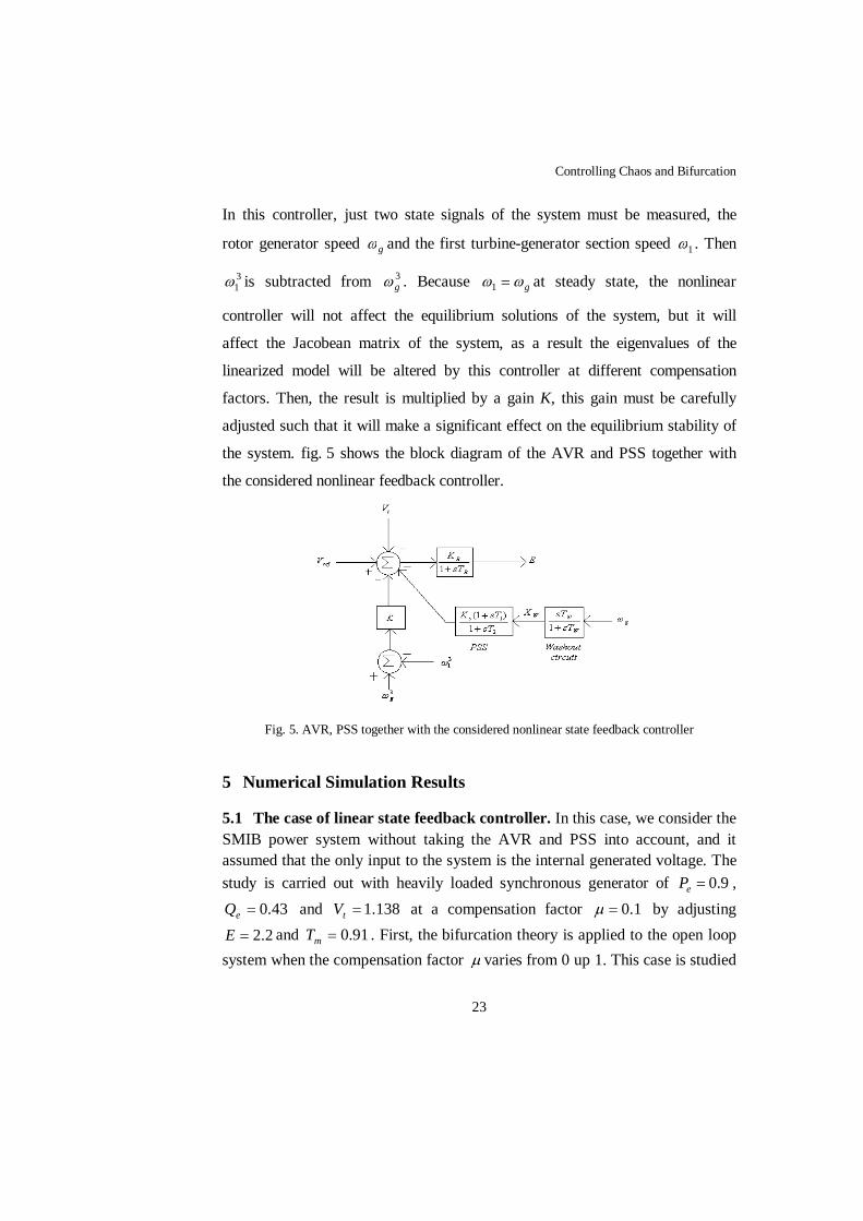
In this controller, just two state signals of the system must be measured, the

rotor generator speed gω and the first turbine-generator section speed 1ω . Then

31ω is subtracted from 3

gω . Because gωω =1 at steady state, the nonlinear

controller will not affect the equilibrium solutions of the system, but it will

affect the Jacobean matrix of the system, as a result the eigenvalues of the

linearized model will be altered by this controller at different compensation

factors. Then, the result is multiplied by a gain K, this gain must be carefully

adjusted such that it will make a significant effect on the equilibrium stability of

the system. fig. 5 shows the block diagram of the AVR and PSS together with

the considered nonlinear feedback controller.

Fig. 5. AVR, PSS together with the considered nonlinear state feedback controller

5 Numerical Simulation Results

5.1 The case of linear state feedback controller. In this case, we consider the SMIB power system without taking the AVR and PSS into account, and it assumed that the only input to the system is the internal generated voltage. The study is carried out with heavily loaded synchronous generator of 9.0=eP ,

43.0=eQ and 138.1=tV at a compensation factor 1.0=µ by adjusting 2.2=E and 91.0=mT . First, the bifurcation theory is applied to the open loop

system when the compensation factor µ varies from 0 up 1. This case is studied


24

in details by Harb and Widyan [36], in which we have 15 differential equations (1)–(15). The 15×15 Jacobean matrix is obtained and the stability of the operating point is studied by monitoring the eigenvalues of the linearized version.

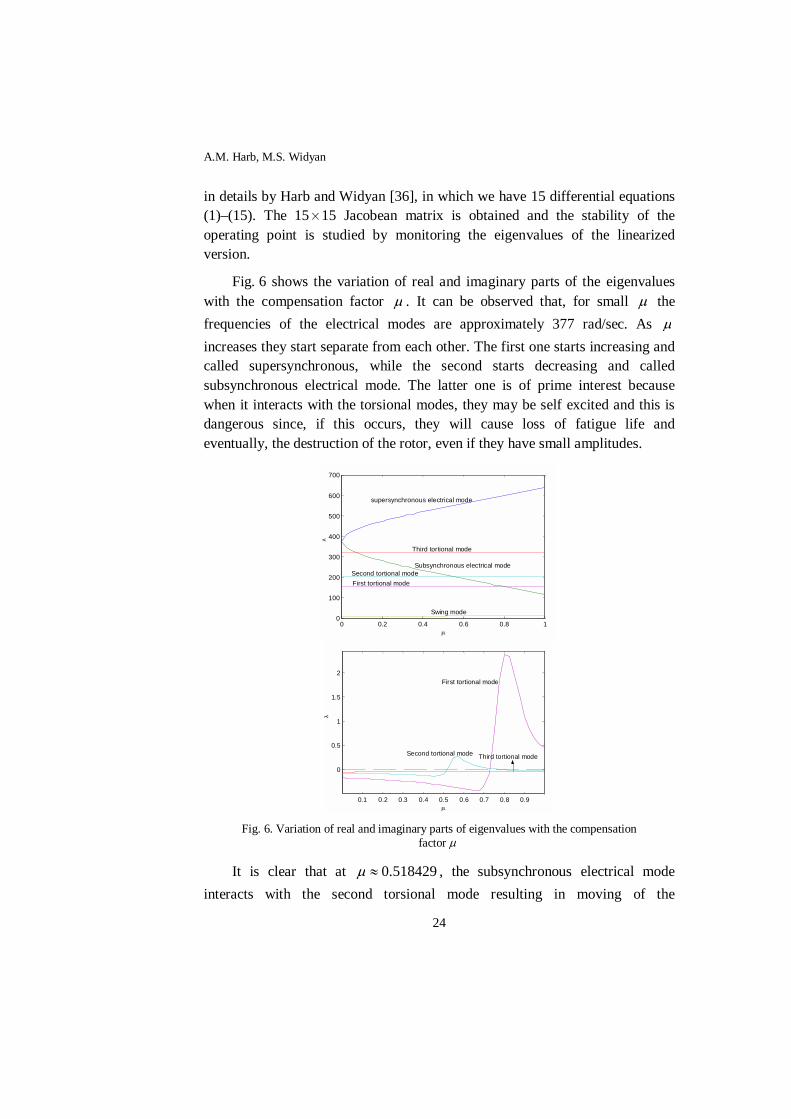
Fig. 6 shows the variation of real and imaginary parts of the eigenvalues with the compensation factor µ . It can be observed that, for small µ the frequencies of the electrical modes are approximately 377 rad/sec. As µ increases they start separate from each other. The first one starts increasing and called supersynchronous, while the second starts decreasing and called subsynchronous electrical mode. The latter one is of prime interest because when it interacts with the torsional modes, they may be self excited and this is dangerous since, if this occurs, they will cause loss of fatigue life and eventually, the destruction of the rotor, even if they have small amplitudes.

0 0.2 0.4 0.6 0.8 10

100

200

300

400

500

600

700

µ

λ

supersynchronous electrical mode

Subsynchronous electrical mode

Third tortional mode

Second tortional mode First tortional mode

Swing mode

0.1 0.2 0.3 0.4 0.5 0.6 0.7 0.8 0.9

0

0.5

1

1.5

2

µ

λ

First tortional mode

Second tortional mode Third tortional mode

Fig. 6. Variation of real and imaginary parts of eigenvalues with the compensation

factor µ

It is clear that at 518429.0≈µ , the subsynchronous electrical mode interacts with the second torsional mode resulting in moving of the


25

corresponding real parts of eigenvalues towards the zero axis. Unfortunately, this interaction was strong enough to transversally move the real parts of the corresponding eigenvalues from left- to the right half of the complex plane. Hence, a Hopf bifurcation had been occurred.

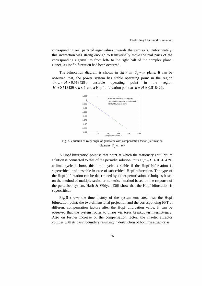
The bifurcation diagram is shown in fig. 7 in µδ −g plane. It can be observed that, the power system has stable operating point in the region

518429.00 ≈<< Hµ , unstable operating point in the region 1518429.0 ≤<≈ µH and a Hopf bifurcation point at 518429.0≈= Hµ .

0.4 0.45 0.5 0.55 0.6 0.650.96

0.965

0.97

0.975

0.98

0.985

0.99

0.995

1

1.005

Compensation factor µ

H

Solid Line: Stable operating point Dashed Line: Unstable operating point H: Hopf bifurcation point

Fig. 7. Variation of rotor angle of generator with compensation factor (Bifurcation

diagram, gδ vs. µ )

A Hopf bifurcation point is that point at which the stationary equilibrium solution is connected to that of the periodic solution, thus at 518429.0≈= Hµ , a limit cycle is born, this limit cycle is stable if the Hopf bifurcation is supercritical and unstable in case of sub critical Hopf bifurcation. The type of the Hopf bifurcation can be determined by either perturbation techniques based on the method of multiple scales or numerical method based on the response of the perturbed system. Harb & Widyan [36] show that the Hopf bifurcation is supercritical.

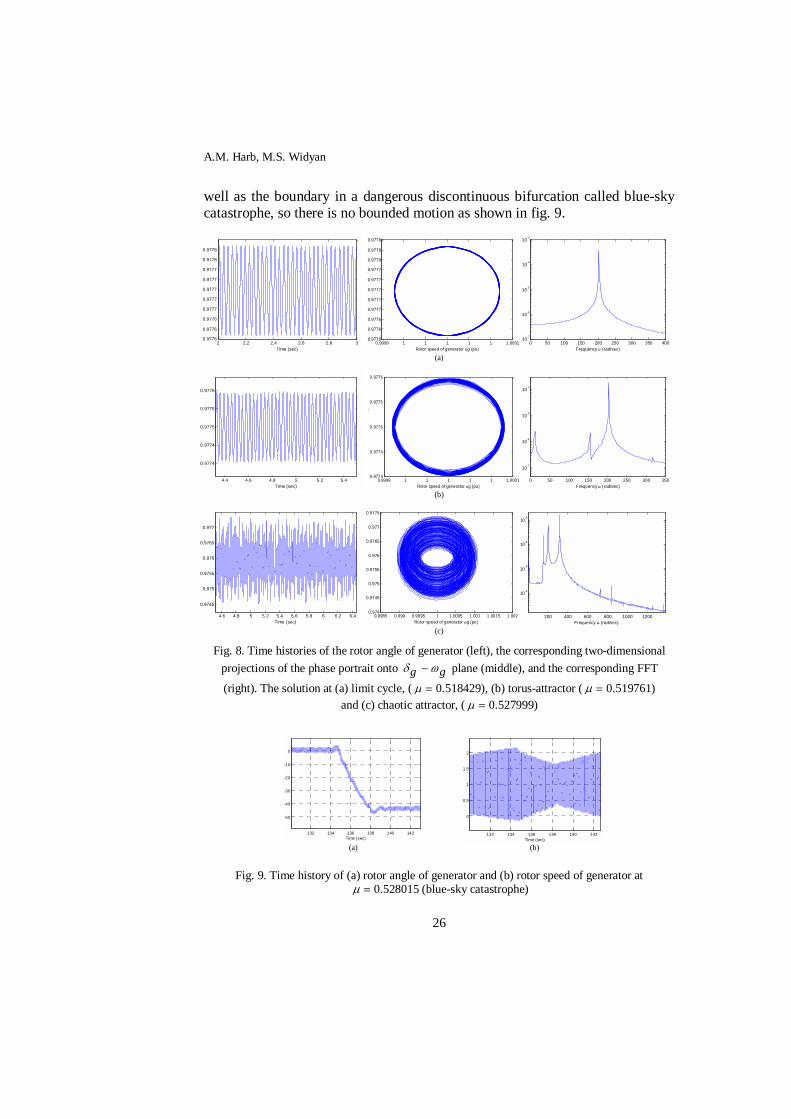
Fig. 8 shows the time history of the system emanated near the Hopf bifurcation point, the two-dimensional projection and the corresponding FFT at different compensation factors after the Hopf bifurcation value. It can be observed that the system routes to chaos via torus breakdown intermittency. Also on further increase of the compensation factor, the chaotic attractor collides with its basin boundary resulting in destruction of both the attractor as


26

0.9999 1 1 1 1 1 1.00010.9776

0.9776

0.9776

0.9777

0.9777

0.9777

0.9777

0.9777

0.9778

0.9778

0.9778

Rotor speed of generator ωg (pu)

δ

0.9999 1 1 1 1 1 1.00010.9774

0.9774

0.9775

0.9775

0.9776


δ

0.9985 0.999 0.9995 1 1.0005 1.001 1.0015 1.0020.974

0.9745

0.975

0.9755

0.976

0.9765

0.977

0.9775


well as the boundary in a dangerous discontinuous bifurcation called blue-sky catastrophe, so there is no bounded motion as shown in fig. 9.

(a)

(b)

(c)

Fig. 8. Time histories of the rotor angle of generator (left), the corresponding two-dimensional projections of the phase portrait onto gg ωδ − plane (middle), and the corresponding FFT

(right). The solution at (a) limit cycle, ( =µ 0.518429), (b) torus-attractor ( =µ 0.519761) and (c) chaotic attractor, ( =µ 0.527999)

(a) (b)

Fig. 9. Time history of (a) rotor angle of generator and (b) rotor speed of generator at =µ 0.528015 (blue-sky catastrophe)

0 50 100 150 200 250 300 350 40010-7

10-6

10-5

10-4

10-3

Frequency ω (rad/sec)2 2.2 2.4 2.6 2.8 3

0.9776

0.9776

0.9776

0.9777

0.9777

0.9777

0.9777

0.9777

0.9778

0.9778

Time (sec)

δ

4.4 4.6 4.8 5 5.2 5.4

0.9774

0.9774

0.9775

0.9775

0.9776

Time (sec)0 50 100 150 200 250 300 350

10-7

10-6

10-5

10-4

Frequency ω (rad/sec)

4.6 4.8 5 5.2 5.4 5.6 5.8 6 6.2 6.4

0.9745

0.975

0.9755

0.976

0.9765

0.977

Time (sec)200 400 600 800 1000 1200

10-6

10-5

10-4

10-3

Frequency ω (rad/sec)

132 134 136 138 140 142

-50

-40

-30

-20

-10

0

Time (sec)132 134 136 138 140 142

0

0.5

1

1.5

2

Time (sec)


27

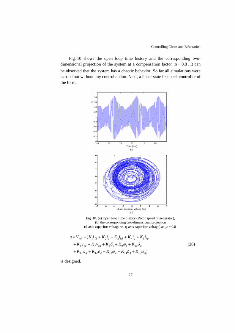
Fig. 10 shows the open loop time history and the corresponding two-dimensional projection of the system at a compensation factor 8.0=µ . It can be observed that the system has a chaotic behavior. So far all simulations were carried out without any control action. Next, a linear state feedback controller of the form:

14 15 16 17 18 190

0.2

0.4

0.6

0.8

1

1.2

1.4

1.6

1.8

Time (sec)

ω

(a)

-8 -6 -4 -2 0 2 4 6 8-8

-6

-4

-2

0

2

4

6

d-axis capacitor voltage (pu) (b)

Fig. 10. (a) Open loop time history (Rotor speed of generator), (b) the corresponding two-dimensional projection

(d-axis capacitor voltage vs. q-axis capacitor voltage) at 8.0=µ

)

(

31531421321211

10191876

54321

ωδωδω

δωδ

KKKKKKKKvKvK

iKiKiKiKiKVu

g

gcqcd

kqqkddfdref

+++++

+++++

++++−=

(28)

is designed.


28

Now, the objective is to find the constant gains ( 151 KK � ) such that the linearized model around the operating point has the desired eigenvalues of:

=P i60012 ±− , i3215±− , i2044 ±− , i15512 ±− , i1606±− , 30− , i115±− , 5− , 10− .

The MATLAB built in function ),,( PBAplaceK = is used to find the designed gains ( 151 KK � ), and the following result is obtained

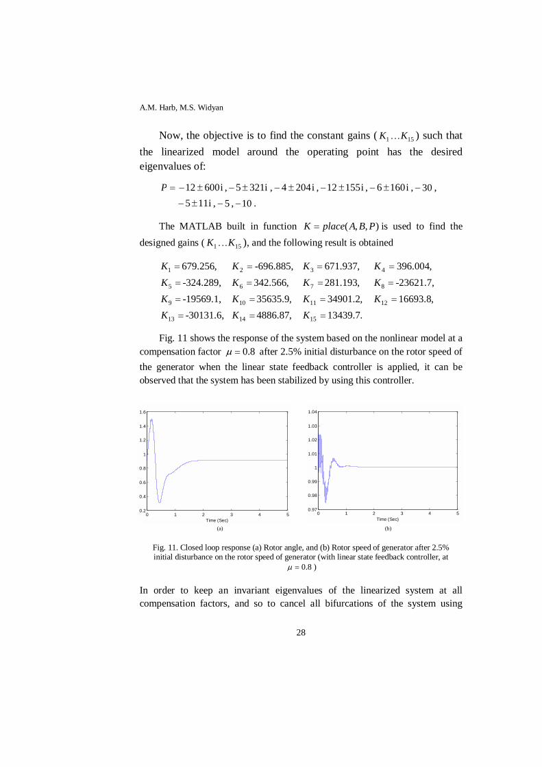
=1K 679.256, =2K -696.885, =3K 671.937, =4K 396.004, =5K -324.289, =6K 342.566, =7K 281.193, =8K -23621.7, =9K -19569.1, =10K 35635.9, =11K 34901.2, =12K 16693.8, =13K -30131.6, =14K 4886.87, =15K 13439.7.

Fig. 11 shows the response of the system based on the nonlinear model at a compensation factor 8.0=µ after 2.5% initial disturbance on the rotor speed of the generator when the linear state feedback controller is applied, it can be observed that the system has been stabilized by using this controller.

(a) (b)

Fig. 11. Closed loop response (a) Rotor angle, and (b) Rotor speed of generator after 2.5% initial disturbance on the rotor speed of generator (with linear state feedback controller, at

8.0=µ )

In order to keep an invariant eigenvalues of the linearized system at all compensation factors, and so to cancel all bifurcations of the system using

0 1 2 3 4 50.2

0.4

0.6

0.8

1

1.2

1.4

1.6

Time (Sec)0 1 2 3 4 5

0.97

0.98

0.99

1

1.01

1.02

1.03

1.04

Time (Sec)


29

linear state feedback controller, one must vary the controller gains at all compensation factors, and before that one must check the controllability of the system at every compensation factor.

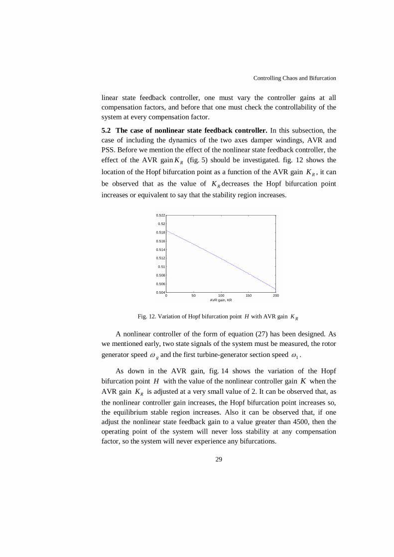
5.2 The case of nonlinear state feedback controller. In this subsection, the case of including the dynamics of the two axes damper windings, AVR and PSS. Before we mention the effect of the nonlinear state feedback controller, the effect of the AVR gain RK (fig. 5) should be investigated. fig. 12 shows the location of the Hopf bifurcation point as a function of the AVR gain RK , it can be observed that as the value of RK decreases the Hopf bifurcation point increases or equivalent to say that the stability region increases.

0 50 100 150 2000.504

0.506

0.508

0.51

0.512

0.514

0.516

0.518

0.52

0.522

AVR gain, KR

Fig. 12. Variation of Hopf bifurcation point H with AVR gain RK

A nonlinear controller of the form of equation (27) has been designed. As we mentioned early, two state signals of the system must be measured, the rotor generator speed gω and the first turbine-generator section speed 1ω .

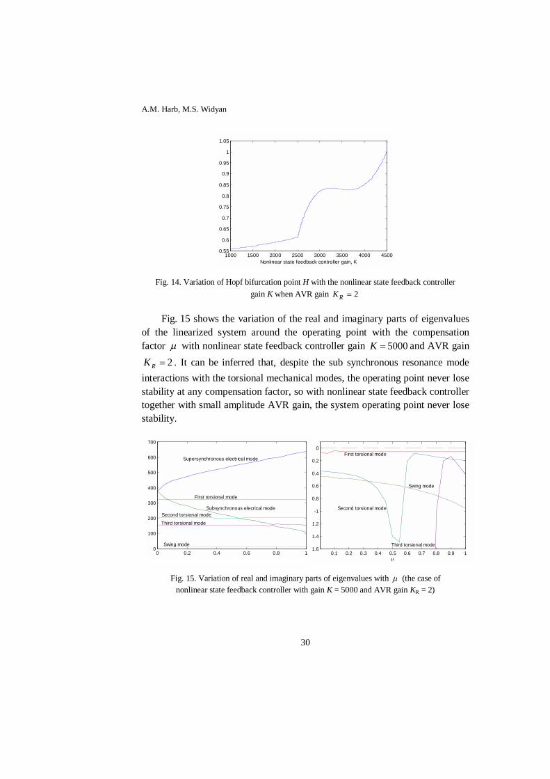
As down in the AVR gain, fig. 14 shows the variation of the Hopf bifurcation point H with the value of the nonlinear controller gain K when the AVR gain RK is adjusted at a very small value of 2. It can be observed that, as the nonlinear controller gain increases, the Hopf bifurcation point increases so, the equilibrium stable region increases. Also it can be observed that, if one adjust the nonlinear state feedback gain to a value greater than 4500, then the operating point of the system will never loss stability at any compensation factor, so the system will never experience any bifurcations.


30

1000 1500 2000 2500 3000 3500 4000 45000.55

0.6

0.65

0.7

0.75

0.8

0.85

0.9

0.95

1

1.05

Nonlinear state feedback controller gain, K

Fig. 14. Variation of Hopf bifurcation point H with the nonlinear state feedback controller gain K when AVR gain 2=RK

Fig. 15 shows the variation of the real and imaginary parts of eigenvalues of the linearized system around the operating point with the compensation factor µ with nonlinear state feedback controller gain 5000=K and AVR gain

2=RK . It can be inferred that, despite the sub synchronous resonance mode interactions with the torsional mechanical modes, the operating point never lose stability at any compensation factor, so with nonlinear state feedback controller together with small amplitude AVR gain, the system operating point never lose stability.

Fig. 15. Variation of real and imaginary parts of eigenvalues with µ (the case of nonlinear state feedback controller with gain K = 5000 and AVR gain KR = 2)

0.1 0.2 0.3 0.4 0.5 0.6 0.7 0.8 0.9 11.6

1.4

1.2

-1

0.8

0.6

0.4

0.2

0

µ

First torsional mode

Swing mode

Second torsional mode

Third torsional mode

0 0.2 0.4 0.6 0.8 10

100

200

300

400

500

600

700

Supersynchronous electrical mode

Subsynchronous elecrical mode

First torsional mode

Second torsional mode

Third torsional mode

Swing mode


31

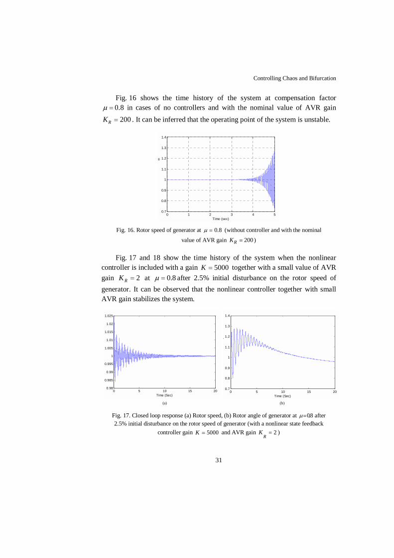
Fig. 16 shows the time history of the system at compensation factor =µ 0.8 in cases of no controllers and with the nominal value of AVR gain

200=RK . It can be inferred that the operating point of the system is unstable.

0 1 2 3 4 50.7

0.8

0.9

1

1.1

1.2

1.3

1.4

Time (sec)

ω

Fig. 16. Rotor speed of generator at 8.0=µ (without controller and with the nominal

value of AVR gain 200=RK )

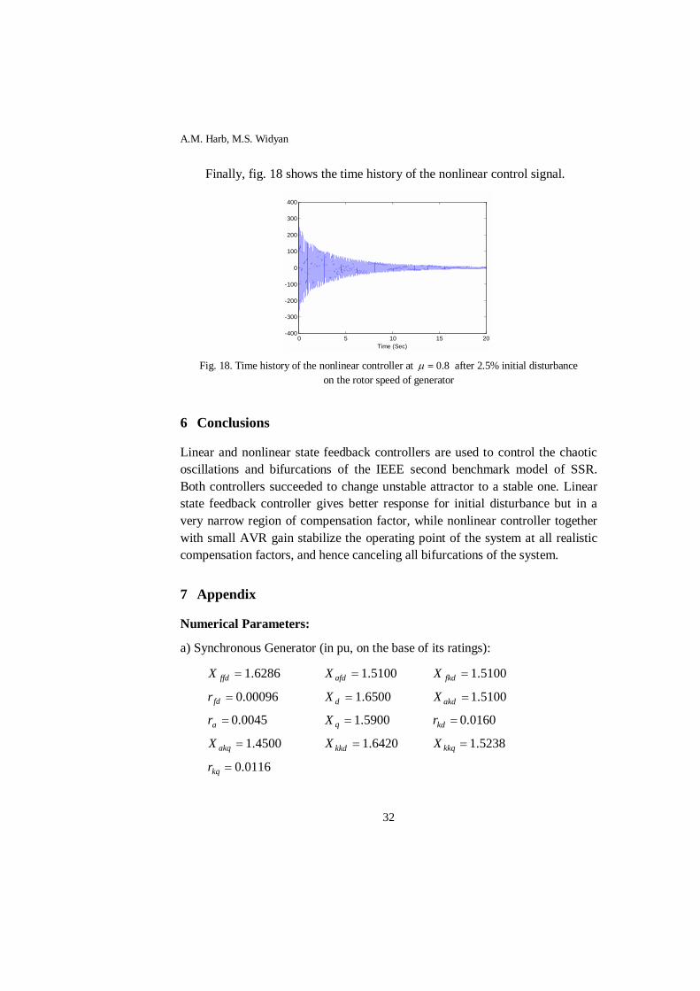
Fig. 17 and 18 show the time history of the system when the nonlinear controller is included with a gain 5000=K together with a small value of AVR gain 2=RK at 8.0=µ after 2.5% initial disturbance on the rotor speed of generator. It can be observed that the nonlinear controller together with small AVR gain stabilizes the system.

(a) (b)

Fig. 17. Closed loop response (a) Rotor speed, (b) Rotor angle of generator at 8.0=µ after 2.5% initial disturbance on the rotor speed of generator (with a nonlinear state feedback

controller gain 5000=K and AVR gain 2=

RK )

0 5 10 15 200.98

0.985

0.99

0.995

1

1.005

1.01

1.015

1.02

1.025

Time (Sec)0 5 10 15 20

0.7

0.8

0.9

1

1.1

1.2

1.3

1.4

Time (Sec)

δ


32

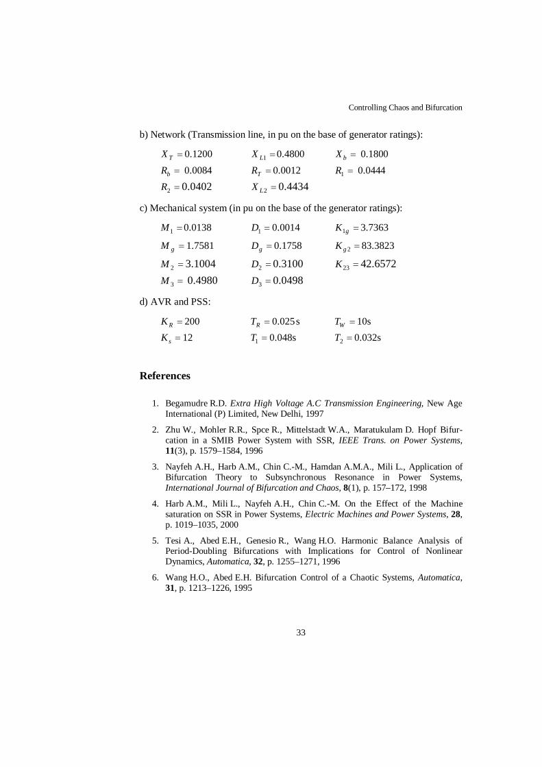
Finally, fig. 18 shows the time history of the nonlinear control signal.

0 5 10 15 20-400

-300

-200

-100

0

100

200

300

400

Time (Sec) Fig. 18. Time history of the nonlinear controller at 8.0=µ after 2.5% initial disturbance

on the rotor speed of generator

6 Conclusions

Linear and nonlinear state feedback controllers are used to control the chaotic oscillations and bifurcations of the IEEE second benchmark model of SSR. Both controllers succeeded to change unstable attractor to a stable one. Linear state feedback controller gives better response for initial disturbance but in a very narrow region of compensation factor, while nonlinear controller together with small AVR gain stabilize the operating point of the system at all realistic compensation factors, and hence canceling all bifurcations of the system.

7 Appendix

Numerical Parameters:

a) Synchronous Generator (in pu, on the base of its ratings):

=ffdX 1.6286 =afdX 1.5100 =fkdX 1.5100

=fdr 0.00096 =dX 1.6500 =akdX 1.5100

=ar 0.0045 =qX 1.5900 =kdr 0.0160

=akqX 1.4500 =kkdX 1.6420 =kkqX 1.5238

=kqr 0.0116


33

b) Network (Transmission line, in pu on the base of generator ratings):

=TX 0.1200 =1LX 0.4800 =bX 0.1800 =bR 0.0084 =TR 0.0012 =1R 0.0444 =2R 0.0402 =2LX 0.4434

c) Mechanical system (in pu on the base of the generator ratings):

=1M 0.0138 =1D 0.0014 =gK1 3.7363

=gM 1.7581 =gD 0.1758 =2gK 83.3823

=2M 3.1004 =2D 0.3100 =23K 42.6572 =3M 0.4980 =3D 0.0498

d) AVR and PSS:

=RK 200 025.0=RT s =WT 10s =sK 12 =1T 0.048s =2T 0.032s

References

1. Begamudre R.D. Extra High Voltage A.C Transmission Engineering, New Age International (P) Limited, New Delhi, 1997

2. Zhu W., Mohler R.R., Spce R., Mittelstadt W.A., Maratukulam D. Hopf Bifur-cation in a SMIB Power System with SSR, IEEE Trans. on Power Systems, 11(3), p. 1579–1584, 1996

3. Nayfeh A.H., Harb A.M., Chin C.-M., Hamdan A.M.A., Mili L., Application of Bifurcation Theory to Subsynchronous Resonance in Power Systems, International Journal of Bifurcation and Chaos, 8(1), p. 157–172, 1998

4. Harb A.M., Mili L., Nayfeh A.H., Chin C.-M. On the Effect of the Machine saturation on SSR in Power Systems, Electric Machines and Power Systems, 28, p. 1019–1035, 2000

5. Tesi A., Abed E.H., Genesio R., Wang H.O. Harmonic Balance Analysis of Period-Doubling Bifurcations with Implications for Control of Nonlinear Dynamics, Automatica, 32, p. 1255–1271, 1996

6. Wang H.O., Abed E.H. Bifurcation Control of a Chaotic Systems, Automatica, 31, p. 1213–1226, 1995


34

7. Abed E.H. Bifurcation-Theoretic Issues in the Control of Voltage Collapse, In: Proc. IMA Workshop on Systems and Control Theory for Power Systems, Chow J.H., Kokotovic P.V., Thomas R.J. (Eds.), Springer, p. 1–21, 1995

8. Chen D., Wang H.O., Chen G. Anti-Control of Hopf Bifurcations Through Washout Filters, In: Proc. 37th IEEE Conf. Decission and Control, Tampa, FL, Dec., 16–18, p. 3040–3045, 1998

9. Chen G., Dong X. From Chaos to Order: Methodologies, Perspectives and Applications, World Scientific, Singapore, 1998

10. Moiola J.L., Chen G. Hopf Bifurcation Analysis: A Frequency Domain Ap-proach, World Scientific, Singapore, 1996

11. Abed E.H., Fu J.H. Local Feedback Stabilization and Bifurcation Control, I. Hopf Bifurcation, Syst. Cont. Lett., 7, p. 11–17, 1986

12. Laufenberg M.J., Pai M.A., Padiyar K.R. Hopf Bifurcation Control in Power Systems with Static VAR Compensator, Int. J. Elect. Power and Energy Syst., 19, p. 339–347, 1997

13. Calandrini G., Paolini E., Moiola J.L., Chen G. Controlling Limit Cycles and Bifurcations, Controlling Chaos and Bifurcations in Engineering Systems, C. Chen G. (Ed.), CRC Press, p. 200–227, 1999

14. Berns D.W., Moiola J.L., Chen G. Feedback Control of Limit Cycle Amplitude from a Frequency Domain Approach, Automatica, 34, 1567-1573, 1998

15. Cam U., Kuntman H. A New CCII-Based Sinusoidal Oscillator Providing Fully Independent Control of Oscillation Condition and Frequency, Microelectron. J., 29, p. 913–919, 1998

16. Basso M., Evangelisti A., Genesio R., Tesi A. On Bifurcation Control in Time Delay Feedback Systems, Int. J. Bifurcation and Chaos, 8, p. 713-721, 1998

17. Alhumaizi K., Elnashaie S.E.H. Effect of Control Loop Configuration on the Bifurcation Behavior and Gasoline Yield of Industrial Fluid Catalytic Cracking (FFC) Units, Math. Comp. Modelling, 25, p. 37–56, 1997

18. Moiola J.L., Desages A.C., Romagnoli J.A. Degenerate Hopf Bifurcation via Feedback System Theory-Higher Order Harmonic Balance, Chem. Eng. Sci., 4, p. 1475–1490, 1991

19. Liaw D.C., Abed E.H. Control of Compressor Stall Inception – A Bifurcation-Theoretic Approach, Automatica, 32, p. 109–115, 1996

20. Gu G., Sparks A.G., Banda S.S. Bifurcation Based Nonlinear Feedback Control for Rotating Stall in Axial Flow Compressors, Int. J. Cont., 6, p. 1241–1257, 1997

21. Ono E., Hosoe S., Tuan H.D., Doi S. Bifurcation in Vehicle Dynamics and Robust Front Wheel steering Control, IEEE Trans. Contr. Syst. Technol., 6, p. 412–420, 1998


35

22. Dobson I., Lu L.M., Computing an Optimal Direction on Control Space to Avoid Saddle-Node Bifurcation and Voltage Collapse, In: Electric Power Systems, IEEE Trans. Auto. Cont., 37, p. 1616–1620, 1992

23. Goman M.G., Khramtsovsky A.V. Application of Continuation and Bifurcation Methods to the Design of Control systems, Phil. Trans. R. Soc. Lond., A356, p. 2277–2295, 1998

24. Moroz I.M., Baigent S.A., Clayton F.M., Lever K.V. Bifurcation Analysis of the Control of an Adaptive Equalizer, In: Proc. R. Soc. London, Series A-Math. And Phys. Sciences, 537, p. 501–515, 1992

25. Senjyu T., Uezato K. Stability Analysis and Suppression Control of Rotor Oscillation for Stepping Motors by Lyapunov Direct Method, IEEE Trans. Power Electron, p. 333–339, 1995

26. Srivastava K.N., Srivastava S.C. Application of Hopf Bifurcation Theory for Determining Critical Value of a Generator Control or Load Parameter, Int. J. Electrical Power Energy Syst., 17, p. 347–354, 1995

27. Ueta T., Kawakami H., Morita I. A Study of the Pendulum Equation With a Periodic Impulse Force-Bifurcation and Chaos, IEICE Trans. Fundam Electr. Commun. Comput. Sci. E78A, p. 1269–1275, 1995

28. Volkov A.N., Zagashvili U.V. A Method of Synthesis for Automatic Control Systems with Maximum Degree of Stability and Given Oscillation Index, J. Comput. Systs. Sci. Int., 36, p. 29–34, 1997

29. Hassard B., Jiang K. Unfolding a Point of Degenerate Hopf Bifurcation in an Enzyme-Catalyzed Reaction Model, Siam J. Math. Anal., 23, p. 1291–1304, 1992

30. Hu G., Haken H. Potential of the FokkerPlank Equation at Degenerate Hopf Bifurcation Points, Phys. Rev. A41, p. 2231–2234, 1990

31. Iida S.K., Ogawara K., Furusawa S.A. Study on Bifurcation Control Using Pattern Recognition of Thermal Convection, JSME Int. J. Series B-Fluid and Thermal Eng., 39, p. 762–767, 1996

32. Reznik D., Scholl E. Oscillation Modes, Transient Chaos and its Control in Modulation-Doped Semi-Conductor Double-Heterostructure, Zeitschrift fur physik B-Condensed matter, 91, p. 309–316, 1993

33. Malmgren B.A., Winter A., Chen D.L. El Nino Southern Oscillation and North Atlantic Oscillation Control of Climate in Puerto Rico, J. Climate, 11, p. 2713–2717, 1998

34. Abed E.H., Wang H.O., Chen R.C. Stabilization of Period Doubling Bifurcations and Implications for Control of Chaos, Physica. D70, p. 154–164, 1994

35. Yabuno H. Bifurcation Control of Parametrically Excited Duffing System By a Combined Linear-Plus-Nonlinear Feedback Control, Nonlin. Dyn., 12, p. 264–274, 1997


36

36. Harb A.M., Widyan M.S. Chaos and Bifurcation as Applied to Subsynchronous Resonance of the IEEE Second Benchmark Model, submitted to Electric Power Components and Systems.

37. Saadat H. Power System Analysis, McGraw Hill, 1999

controlling chaos and bifurcation of subsynchronous resonance in … · · 2012-06-22controlling...

Documents