Technical University Delft

Faculty of Civil Engineering and Geosciences

PLASTICITY Ct 4150 The plastic behaviour and the calculation of plates subjected to bending Prof. ir. A.C.W.M. Vrouwenvelder Prof. ir. J. Witteveen March 2003 Ct 4150

Preface

Course CT4150 is a Civil Engineering Masters Course in the field of Structural Plasticity for building types of structures. The course covers both plane frames and plates. Although most students will already be familiar with the basic concepts of plasticity, it has been decided to start the lecture notes on frames from the very beginning. Use has been made of rather dated but still valuable course material by Prof. J. Stark and Prof, J. Witteveen. After the first introductory sections the notes go into more advanced topics like the proof of the upper and lower bound theorems, the normality rule and rotation capacity requirements. The last chapters are devoted to the effects of normal forces and shear forces on the load carrying capacity, both for steel and for reinforced concrete frames. The concrete shear section is primarily based on the work by Prof. P. Nielsen from Lyngby and his co-workers. The lecture notes on plate structures are mainly devoted to the yield line theory for reinforced concrete slabs on the basis of the approach by K. W. Johansen. Additionally also consideration is given to general upper and lower bound solutions, both for steel and concrete, and the role plasticity may play in practical design. From the theoretical point of view there is ample attention for the correctness and limitations of yield line theory for reinforced concrete plates on the one side and von Mises and Tresca type of materials on the other side. This, however, is not intended for examination. I would like to thank ir Cox Sitters for his translation of the original Dutch text into English as well as for his many suggestions for improvements. A. Vrouwenvelder Delft, 2003

Table of contents Preface Notation ................................................................................................................................. 2 1 Introduction....................................................................................................................... 4 2 Elastic-plastic behaviour of a plate Lower- and upper-bound theorems................................................................................... 5

2.1 Behaviour of a plate under increasing load ............................................................. 5 2.2 The upper-bound theorem ....................................................................................... 6 2.3 The lower-bound theorem ....................................................................................... 6 2.4 Validity of the theorems .......................................................................................... 6

3 Yield-line theory ............................................................................................................... 7

3.1 Material behaviour .................................................................................................. 7 3.2 Yield-line theory...................................................................................................... 7 3.3 Yield-line pattern..................................................................................................... 7 3.4 The work equation................................................................................................... 8

4 Simply-supported rectangular plate ................................................................................ 11

4.1 Rectangular plate with length twice the width (b = 2a) ........................................ 11 4.2 Additional formulae .............................................................................................. 12 4.3 Rectangular plate with arbitrarily chosen dimensions (b = �a) ............................ 14 4.4 Some examples...................................................................................................... 16

5 Lower-bound calculation and design methods ............................................................... 18

5.1 Equilibrium equation and conditions .................................................................... 18 5.2 The twistless case .................................................................................................. 22 5.3 Design in accordance with the theory of plasticity ............................................... 22

6 Alternative upper-bound calculation (direct formulation of the equilibrium of the plate parts) ............................................... 25

6.1 Equivalent nodal forces and moments................................................................... 25 6.2 Minimisation of the load factor ............................................................................. 27

7 The rectangular restrained plate...................................................................................... 29

7.1 Upper-bound solution............................................................................................ 29 7.2 Lower-bound solution ........................................................................................... 30 7.3 Approximation of yield zones ............................................................................... 31

8 Simply supported square plate with two free edges ....................................................... 35

8.1 Some upper-bound solutions ................................................................................. 35 8.2 Elastic solution ...................................................................................................... 38

1

9 Circular plates ................................................................................................................. 39 9.1 Uniform load on a simply supported circular plate ............................................... 39 9.2 Uniform load on a restrained circular plate........................................................... 42 9.3 Point load in the centre of a simply supported circular plate ................................ 43 9.4 Point load in the centre of a restrained circular plate ............................................ 44

10 Point loads and simple supports on columns .................................................................. 46

10.1 Point load in the centre of a simply supported square plate .................................. 46 10.2 Point load in the centre of a restrained square plate.............................................. 46 10.3 Infinitely long simply supported plate................................................................... 47 10.4 Point load on free edges and free corners.............................................................. 49 10.5 Plate on columns ................................................................................................... 51

11 Yield criteria of the largest principal moment, Tresca and von Mises ........................... 54

11.1 General formulation of yield criterion................................................................... 54 11.2 The yield criterion of the largest principal moment (square yield criterion) ........ 54 11.3 The yield criterion of Tresca ................................................................................. 56 11.4 The yield criterion of von Mises (Huber, Hencky) ............................................... 57 11.5 Lower-bound calculation of a torsion panel.......................................................... 58

12 Yield criterion for reinforced concrete slabs .................................................................. 60

12.1 Yield line in x- or y-direction ................................................................................ 60 12.2 Yield line under an angle with the y direction....................................................... 61 12.3 Yield line calculation of reinforced concrete torsion panel .................................. 63 12.4 Yield criterion formulated in moments with respect to the x-y system................. 64 12.5 Example: lower-bound calculation of reinforced concrete torsion panel.............. 69 12.6 Example: design calculation.................................................................................. 71

13 General background on plastic calculation of plates ...................................................... 74

13.1 Further description of ideal-plastic material behaviour ........................................ 74 13.2 General procedure for the upper-bound calculation.............................................. 76 13.3 Yield criterion for reinforced concrete slabs – additional considerations............. 83

14 Final considerations ........................................................................................................ 93 Literature......................................................................................................................... 95 Appendix A: Formulae for plates ................................................................................... 97 Appendix B: Transformation formulae for plate moments .......................................... 100 Questions ...................................................................................................................... 101 Answers to question 1 – 16........................................................................................... 111

2

0 Notation Notation of symbols a,b - plate dimensions e1, e2, … - strain parameters Ed - dissipated energy during plastic deformation F - point load Fi - resultant of interaction forces h - thickness of plate K - constant lx, ly - absolute co-ordinate differences mxx, mxy, myy - plate moments mI, mII - principal moments mp - plastic moment of plate (or yield, ultimate, limit moment)

,px pym m - positive plastic moments in reinforcement direction ,px pym m� � - negative plastic moments in reinforcement direction

n, s, z� - local cartesian co-ordinate system at yield line q - surface load qx, qy - transverse forces R - radius of circle r, �, z - cylinder co-ordinate directions s1, s2, … - stress parameters w - displacement centre plane of plate wz - displacement centre of gravity of plate part w - displacement of a point of reference W - work performed by external load x, y, z - cartesian co-ordinate directions �, �, � - ratio factors, angles �� - load factor �p - ultimate load factor (load factor at failure) �e - load factor causing initial yielding (subscript e = elastic) �xx, �xy, �yy - curvatures - yield function x, y - rotations

,x y� � - percentages of lower reinforcement ,x y� �� � - percentages of upper reinforcement , ,xx xy yy� � � - stresses

, ,c c cxx xy yy� � � - concrete stresses

, ,s s sxx xy yy� � � - steel stresses , ,I II III� � � - principal stresses

p - yield stress (subscript p = plastic)

3

Notation in figures - free edge of a plate - simply supported edge of a plate - restrained edge of a plate - positive yield line - negative yield line - positive moments and transverse forces

mxy myx

qy

qx mxx

myy

x

y z

4

1 Introduction Application of the principles and propositions of the theory of plasticity is not restricted to beam constructions only. It is possible to extend the theory to two- and three-dimensional continua. For the civil engineer the analysis of plates subjected to bending is of prime importance. In the application of the theory of plasticity three different solution techniques can be distinguished: 1. The incremental (stepwise) elastic-plastic calculation; 2. Application of the lower-bound theorem, which is based on the equilibrium equations

(equilibrium system); 3. Application of the upper-bound theorem, which is based on a mechanism. The computational approach of these three methods is quite different. Normally the incremental calculation cannot be carried out by hand because of its complexity. The use of a computer is required, which often leads to high computational times and costs. Manual application of the lower-bound theorem in order to check existing constructions is difficult too. However, for design calculations the lower-bound method is quite useful. The upper-bound theorem is quite well developed, especially for the application of reinforced concrete slabs. The calculation procedure is known as the yield-line theory. A yield line in a plate is similar to a plastic hinge in a frame. The Dane K.W. Johansen can be regarded as the founding father of the theory. In 1943 he published a Ph.D. thesis on this subject, which later attracted wide attention ([1], [2]). At the same time a number of important developments took place in the general theory of plasticity for continua ([3], [4], [5]). With this new theory a number of intuitive aspects of the yield-line theory could be given a proper theoretical foundation. The fact that the yield-line theory only provides upper-bound solutions forms a restriction for the application on arbitrary practical problems. However, by experimental and theoretical research this shortcoming has been removed to a large extend.

5

2 Elastic-plastic behaviour of a plate Lower- and upper-bound theorems In this chapter the general failure behaviour of a plate will be discussed and a brief introduction will be given on the theory to analyse this type of failure phenomena. 2.1 Behaviour of a plate under increasing load Fig. 2.1a shows a simply supported rectangular plate with sides a and b (see “Notation”) which is loaded by a uniformly distributed load �q (q is a fixed value, � is the load factor). The material is assumed to be elastic ideal-plastic. In unloaded state the plate is stress free. Starting from this unloaded state (� = 0) the load is gradually increased. In first instance the response of the plate is completely elastic. At a certain load factor (� = �e) somewhere in the plate the stress state satisfies the yield condition (Fig. 2.1b), and initial plastic

yielding occurs. When the load is increased the stresses do not increase anymore, or they just change in the way permitted by the yield criterion. The generated plastic deformations are permanent and do not disappear after unloading. During continuing loading more plastic points appear. These points chain together to form lines and zones (Fig. 2.1c). Finally a pattern of yield lines and yield zones is generated such that the plate deflects unlimited, just because of the increasing plastic deformation. During this plastic failure process the elastic deformations, the stresses and also the

a

b

�q

a) rectangular plate with edges a and b and uniformly distributed load �q

b) start of yielding in the middle of the plate: � = �e

c) advanced yielding: �e < � < �p

d) state of failure: � = �p

Fig. 2.1: Behaviour of a rectangular plate under increasing load.

A

A

B

B

A - A B - B

C C

C - C

6

external load remain constant (geometrical non-linear effects are neglected). In this way a mechanism is created and the maximum load carrying capacity (� = �p) is reached (Fig. 2.1d). 2.2 The upper-bound theorem If the shape of the failure mechanism is known, the failure load can directly be obtained with the principle of virtual work. On a plate in state of failure a small plastic deformation is imposed and the resulting work performed by the external loads and the internally dissipated energy are calculated. The load factor � for which the calculated values are the same is the ultimate load factor �p (p = plastic). Normally the actual shape of the failure mechanism is unknown. Therefore, a certain mechanism is assumed and the corresponding load factor is calculated. When this exercise is repeated for all possible mechanisms, then the smallest of all calculated load factors has to be equal to �p. Above statement actually is a description of the upper-bound theorem as formulated in the theory of plasticity, i.e.:

When for an arbitrary mechanism a (positive) load factor � is determined by equating the dissipated energy and the work performed by the external load. Then the found � is an upper bound for the load factor at failure.

It can also be said that a given load factor � is smaller than �p, if not one single mechanism can be found for which the external work is greater than or equal to the dissipated energy. 2.3 The lower-bound theorem As shown above in the upper-bound approach focuses on the displacement field. In the second important proposition of the theory of plasticity the formulation of the stress field is the key issue. The definition reads:

When it is possible to formulate a stress distribution without causing any plastic flow, which is in equilibrium with the external load �q, then � is a lower bound for the load factor at failure �p.

It can also be said that a given load factor � is larger than �p, if not one single stress distribution can be found, which is in equilibrium with the external load and satisfies all yield criteria. When for a certain load �q it is possible to indicate both a mechanism and a permissible stress field, then the exact solution has been found and the load factor � equals precisely the load factor causing failure �p. 2.4 Validity of the theorems It can be shown that the upper-bound and the lower-bound theorems (also indicated as the propositions of Prager) are not generally valid. Only for special classes of materials the theorems can be applied. However, for now it is assumed that the material used has the desired properties. More attention to this topic will be paid in chapter 13.

7

3 Yield-line theory The yield line theory is quite well developed. Especially the application on reinforced concrete slabs is popular. The fact that the yield-line theory only provides an upper-bound solution is no restriction for practical applications, because the solutions have been validated thoroughly by both experimental and theoretical research. 3.1 Material behaviour During the discussion about the several computational principles it is assumed that the considered plates have very simple plastic properties. The yield criterion is solely based on bending moments. Plastic rotation (in a certain point about a certain line) can occur only if the corresponding bending moment is equal to the plastic moment mp, also indicated by yield moment or ultimate moment. Naturally, the bending moment and the rotation must have the same sign. This yield criterion is quite satisfactory for orthogonal reinforced concrete slabs, which at the top and the bottom in both directions have the same percentage of reinforcement. Since bending and torsion in plates are measured per unit of length, the unit of the yield moment is force and is expressed in Nm/m or shortly N. 3.2 Yield-line theory The first step in the execution of an upper-bound calculation is the choice of a suitable mechanism. In principle each arbitrarily chosen continuous distribution of bending displacements can be considered (the continuity condition is related to the neglect of the transverse force in the yield criterion). The essential characteristic of the yield-line theory however is that the mechanism is chosen such that it only consists out of yield lines. Zones of yielding are not considered. This restriction however is not essential, because any yield zone can be approximated as accurate as desired by a fine mesh of yield lines. 3.3 Yield-line pattern During failure it is assumed that the entire increase of plastic deformation is concentrated in a number of yield lines. In the parts of plate bounded by yield lines and plate edges, the plastic deformation does not change. Since, the elastic deformation also remains constant, these parts of the plate behave like rigid bodies. On basis of the geometrical linear character of the whole calculation the plate parts can be considered to be flat. Summarising the following proposition can be stated: For a pure yield line mechanism the parts of the plate bounded by yield lines and plate

edges behave like rigid flat bodies. It is important to check if each chosen pattern of yield lines satisfies above condition. As an illustration a number of yield line patterns will be investigated for the simply supported square plate as drawn in Fig. 2.1a. The mistake in Fig 3.1a is quite clear. On bases of the proposition and the required continuity of displacements, a yield line can be seen as intersection two flat planes. Therefore, a yield line has to be straight. The pattern of Fig. 3.1b is conflicting with the proposition too. As soon as point D goes down the points A, B, C and D are no longer situated in a flat plane.

8

The mistake in Fig. 3.1c is less obvious. Note that part ABEF rotates about line AB and part CDEF about line CD. The intersection of both parts therefore has to parallel to AB and CD, and not oblique as drawn in Fig. 3.1c. Fig. 3.1d shows a correct yield line pattern. The intersection EF is parallel to AB, consequently the points A, B, E and F are located in a flat plane. The same holds for the points C, D, E, F. The triangular parts AEC and BDF do not cause any problem, since each arbitrary combination of three points span up a flat plane. 3.4 The work equation After the choice of a suitable mechanism the work equation can be formulated. The equation reads as follows: dW E� (3.1) where W is the work done by the external load and Ed the amount of dissipated energy for a certain prescribed displacement during failure. For the evaluation of both terms a Cartesian co-ordinate system is introduced. The x-y plane coincides with the centre plane of the plate. The z-axis is chosen such that in principle the plate is loaded in positive z-direction (Fig. 3.2). Now the case is considered where the plate is loaded by a continuous surface load �q(x,y). If w(x,y) is the increase in displacement during failure, the amount of work done can be written as:

plate area

( , ) ( , )W q x y w x y dxdy�� �� (3.2)

a) yield lines are not straight b) the points ABCD are not lying in a plane

d) correct pattern of yield lines c) line of intersection EF is not parallel to AB

A B

C D

E F

A B

C D

A

F E

B

C D R

R

Q

Q

P P

R-R Q-Q P-P

Fig. 3.1: Yield lines in a rectangular plate; only case d) provides a proper solution.

9

For a constant surface load q, the property can be used that the displacement field is linear between the yield lines and the plate edges. This means that above integral can be reformulated as a summation over all plate parts:

plate partszW q S w�� � �� (3.3)

where S is the area of a plate part and wz the displacement of the centre of gravity. Energy is dissipated in the yield lines only. Fig. 3.3 shows a yield line in an arbitrarily chosen direction, with a local co-ordinate system nsz� attached to it. The n- and s-axes lie

in the x-y plane. The s-axis coincides with the yield line and the n-axis is perpendicular to it. The z�-axis is parallel to the z-axis. The equilibrium conditions must be formulated for the two plate parts at both sides of the yield lines, and therefore the internal forces and moments (per unit of length) in the yield lines must be determined. They are:

- bending moments mnn - torsional moments mns - transverse forces qn

The plastic deformation equals the difference in rotation of both plate parts about the s-axis: ( 0) ( 0)d d dn n� � �� � � � � This dihedral angle is small, i.e.: tan sind d d� � �� � � � �

displacement w(x,y)

external load q(x,y)

x

y z

Fig. 3.2: Choice of co-ordinate system.

x y

z'

z

n s

�d z'

n s

qn

mnn

mns

Fig. 3.3: Deformations and internal loads in a yield line.

10

Of all interactions only mnn provides a contribution to the energy dissipation. For a yield line it can be written:

along yield lined nn dE m ds�� �� �� (3.4)

Since the yield line can be seen as the intersection between two plate parts, the value of �d is constant. For the specified material having an ultimate plastic moment mp it holds:

if 0if 0

nn p d

nn p d

m mm m

�

�

� � � �

� � � �

where a moment is defined positive if for z < 0 the material is in a state of compression. For the total amount of dissipated energy it now can be written: d p d sE m l�� � � �� (3.5)

where mp is the plastic moment, �d is the dihedral angle between the plate parts and ls the length of the yield line.

11

4 Simply-supported rectangular plate In this chapter the formulae, (3.1), (3.3) and (3.5) will be evaluated for a uniformly loaded simply supported rectangular plate as shown in Fig. 2.1a. The mechanism discussed in chapter 2 (Fig. 3.1d) will be used. Firstly, the problem will be worked out for a plate which length is twice the width. Secondly, some additional formulae will be discussed and finally these formulae will be applied to a rectangular plate of arbitrarily chosen dimensions. 4.1 Rectangular plate with length twice the width (b = 2a) Fig. 4.1 shows the geometry and the nomenclature used in this example. The yield lines AE, BF, DF and CE are chosen completely arbitrarily under an angle of 45o.

The downward displacements of the points E and F are indicated by w . All other displacements will be expressed in this quantity. The first step in the calculation is the determination of the areas and the displacement of the centres of gravity of the plate parts. The results are tabulated below.

Plate part Area Displacement centre of gravity ABEF 23

4 a 49 w

BDF 214 a 1

3 w

The surface load on the plate parts ABEF and BDF delivers exactly half of the total amount of work. From (3.3) it is found:

2 2 23 4 1 1 524 9 4 3 6

W q a w q a w W qa w� � �� �

� � � � � � � � �� �

w

C

A

F E

B

D

G1

a

l1

n s

x

y

45o 29 a

16 a

G2

s n l2

12 a

12 a

12 a1

2 a

�d1

w

w

12 w

14section x a� section x = a

A

E

�d2

section x = y

G1 = centre of gravity ABEF G2 = centre of gravity BDF

Fig. 4.1: Data for yield line calculation of rectangular simply supported plate.

12

For the calculation of the amount of dissipated energy the yield lines FE and EC are considered. The corresponding dihedral angles �d1 and �d2 are indicated in Fig. 4.1. The lengths l1 and l2 of the yield lines can be obtained easily. In both cases the plastic moment is positive. So, the following table can be produced:

Yield line Bending moment Dihedral angle Length FE + mp 4w a a EC + mp 2 2w a 1

2 2a

The contributions of all slanting yield lines are equal. Therefore from (3.5) it follows:

4 4 2 2 122d p p d p

w w aE m a m E m wa a

� � � � � � � � �

Equating the external work to the dissipated energy according to (3.1) leads to:

22

5 72126 5

pp

mqa w m w

qa� �� � �

where � is the desired load factor. This completes the procedure: Starting from a mechanism an upper-bound value for the failure load has been found. The interpretation of the result will be discussed later, when the shape of the plate is varied (b = �a) and also the directions of the slanting yield lines. But firstly some additional formulae will be discussed. 4.2 Additional formulae During the calculation of the work term it is handy to make use of the proposition that the displacement of the centre of gravity of a triangle is equal to one third of the sum of the displacements of its vertices. For proof a triangle ABC is considered with point G being the centre of gravity. If point C is displaced by wC while points A and B remain fixed, then the displacement of point G equals wC /3. Analogously point B can be given a displacement for fixed points A and C, and finally A can be displaced for fixed B and C. Superposition of these three cases leads to:

� �13G A B Cw w w w� � � (4.1)

where wG is the displacement of the centre of gravity of the triangle ABC. It is wise to subdivide polygonal plate parts into triangles after which (4.1) can be applied. For the calculation of the dissipation term the following formula usually is very handy (see Fig. 4.2):

s s x x y yl l l� � �� � � � � (4.2)

13

where �x = x(n>0) � x(n<0), �y = y(n>0) � y(n<0), lx is the projection of ls on the x-axis and ly is the projection of ls on the y-axis. The rotations x and y normally can be determined easily. In order to proof (4.2) a co-ordinate transformation is considered where the rotations (x,y) and therefore also the rotations differences (�x,�y) behave like tensors of the first order:

cos sinsin cos

xn

ys

�� � �

�� � �

�� � �� � � �� � �� � � � �� �� � �

where � is the angle between the n-axis and the x-axis. In this case the back transformation is required, i.e.:

cos sinsin cos

x n

y s

� �� �

� �� �

� ��� � � �� ��� � � �� �� �� � �

Since �n = 0 it holds: sin ; cosx s y s� � � � � �� � � � � � It now can be written:

� �2 2sin cos

sin sin cos coss s s s

s s s s

x x y y

l l

l l

l l

� � � �

� � � � � �

� �

� � � �

� � � �

� � � �

which proves relation (4.2).

ww

w

- �x

�d �y

lx

ly ls

s y n x

Fig. 4.2: Determination of the dihedral angle.

14

4.3 Rectangular plate with arbitrarily chosen dimensions (b = �a) Again the plate of Fig. 2.1 is considered with uniformly distributed load �q and sides a and b. The ratio � = b/a is a variable with � � 1. The distance between point E and side AC is set to �a (see Fig. 4.3). The value of � will be determined such that it minimises the upper-bound value of the load factor �.

The data required for the work equation are gathered in the tables below. For the determination of the work, plate part ABEF is subdivided into two triangles after which (4.1) has been applied. Also in this case the displacement of point E is set to w .

Plate part Area Displacement centre of gravity ABE 1 1

2 2b a� 13 w

EFB 1 12 2( 2 )*b a a�� 2

3 w BDF 1

2 a a�� 13 w

Yield line lx ly x�� y��

FE 2b a�� 0 4w a 0 EC a� 1

2 a 2w a ( )w a� The work done by the external load �q yields:

21 1 1 2 1 12 ( 2 )4 3 4 3 2 3

1 2( )2 3

W q ba w a b a w a w

W qa b a w

� � �

� �

� �� � � � � � � �

� �

� �

The dissipated energy is calculated by making use of (3.5) and (4.2):

( )w a�

2w a4w a

12 w

w

C

A

F

B

D b - 2�a

n s

x

y

s n

12 a

12 a

w

12section x a��

Fig. 4.3: Data for yield line calculation of rectangular simply supported plate.

�a �a b = �a

E

12section x b�

12section y a�

15

2 1( 2 ) 4 42

142

d p p

d p

w w wE m b a m a aa a a

bE m wa

� �

�

�

� � � �� � � � � � � � �� �

� �

� �� ��

�

Equating these two formulae according to (3.1) and introducing b = �a provides the following relation for the load factor:

22

11 2 1 24 8 22 3 2

3

pp

mqa w m w

qa

��� � � � �

�� �

� ��� �� � � �

� � � � � � �� � � � � ��� �

(4.3)

For a given value of � the variable � has to be determined such that � is minimised. Therefore, the values of � that make the function for � stationary are possible candidates. Naturally, those values of � should correspond to physically possible positions of point E. This leads to the following condition:

102

� �� �

The result of this condition is that boundary minima have to be considered too. The desired stationary values can be obtained through:

2

2 2

2 1 2 13 2 3 28 0

23

pmdd qa

� � �� � �

�� �

� �� �� � � �� �� � � � �� �� �� � � �� �

� �� � � �� �� � � �� �

�� �� �� �� �� �

The numerator has to be zero, so:

2

2 1 2 1 03 2 3 2

� � �� �

� �� � � �� � � � �� �� � � �� � �

Multiplication by 6�2 delivers: 2 23 2 4 2 0 4 4 3 0� � �� � �� � �� � � � � � � � � This quadratic equation has two roots, the positive solution of which satisfies the listed condition is given by:

21 3 1

2�

��

� � �

�

16

Boundary extremes do not play any role in this case. Now � is known the load factor � can be determined from (4.3). 4.4 Some examples A number of examples of simply supported plates is displayed in the table below. Type of plate � � 2 / pqa m� Square plate 1 0.5 24.00 Length twice the width; first example 2 0.5 14.40 Length twice the width; optimised solution 2 1

4 ( 13 1) 0.651� � 14.14

Infinitely long plate � 12 3 0.866� 8.00

The optimum solution for a plate the length of which is twice the width is indicated too. Comparison with the results of the first example with � = 2 and � = 0.5 shows that the choice of a mechanism which does not give the lowest value of � not necessarily leads to large mistakes in the load factor. For an infinitely long plate of width a (� � �), the factor � approaches 0.5�3 � 0.866 and the load factor is reduced to the minimum value of 8mp/(qa2). The results are displayed graphically in Fig.4.4.

It can be concluded that the load carrying capacity of the plate increases with decreasing span in x-direction. The maximum is reached for a square plate, which can resist a three times higher failure load than the infinitely long plate.

45o

38o

30o

� = 1

� = 2

� = �

x

y

1 2 3 4 5 6 7 8 9 10

1 2 3 4 5 6 7 8 9 10

�

�

�

2

p

qam�

0.0

0.2

0.4

0.6

0.8

4 0

8 121620

2824

Fig. 4.4: Results for rectangular simply supported plate.

17

Naturally, the found values for � are upper limits, which means that the actual load factor is lower. In most cases one has to accept these solutions, because they are the only ones available. However, for this plate by a lower-bound calculation it can be shown that the calculated excess in load carrying capacity over the whole range is not more than 1%. For � = 1 and � = � even the exact solution is found. The mentioned lower-bound calculation will be given in next chapter. Using the theory discussed so far the questions 1 up to 8 (at the end of this handbook) can be solved. The student is advised to tackle at least some of these problems before continuing with the theory.

18

5 Lower-bound calculation and design methods In this chapter some aspects of the lower-bound calculation will be discussed. Lower-bound solutions are generally not very practical to apply, because of the required computational effort. However, one exception is the use of a lower-bound solution in the design of reinforced concrete slabs. 5.1 Equilibrium equation and conditions For the determination of a lower bound of the load factor �p at failure a moment distribution has to be found for which:

- all equilibrium conditions are satisfied; - the yield criterion is not violated anywhere.

According to the theory for plates ([9], [10], also see appendix A) the equilibrium equation for the plate field is given by:

2 22

2 22 ( , ) 0xy yyxx m mm q x yx x y y

�� ��

� � � �� � � �

(5.1)

Except this field equation the continuity condition and the eventual boundary conditions have to be satisfied too. The most important boundary conditions are those for the free and simply supported edge (a restrained edge does not provide any dynamical boundary

conditions). On the edge a local co-ordinate system nsz� is defined, with the s-axis along the edge and the n-axis pointing inward. In that case the mentioned boundary conditions can be written as: simply supported edge: 0nnm � (5.2)

0

free edge:0

nn

snn

mmqs

���� �

� �� ��

(5.3)

where qn is the distributed transverse load at n = 0 given by:

z�

s n

plate edge

Fig. 5.1: Concentrated shear force at free or simply supported plate edge.

19

nn snn

m mqn s

� �� �

� � (5.4)

The torque mns at a free or simply supported edge causes a special phenomenon. In the theory of plates this torque leads to the so-called concentrated transverse load. The shear stress due to the torsional moment has the tendency to bend around at the plate edge as indicated in Fig. 5.1. The resultant of the vertical shear stresses can be interpreted as a (non-uniform) transverse single force Qs, which after some investigation appears to be of the same magnitude as the torque mns. The increase of this concentrated force in s-direction has to be the same as the supply of transverse load in n-direction. This globally explains the second relation of (5.3). For more information it is referred to [9] and [10]. Remark: In case of an outward-pointing normal n the force Qs will be equal to –mns. The second condition to be satisfied by the moment distribution concerns the yield criterion. Application of the material behaviour as described in chapter 3 requires that the absolute value of the bending moments in all points in each direction are smaller than the plastic moment mp of the plate. Since plate moments can be seen as tensors of the second order it is sufficient to check both principal moments: the largest principal moment has to be smaller than +mp, the smallest principal moment larger than –mp. The formulae for the determination of the principal moments read (also see Fig. 5.2):

� � � �

� � � �

2 2

2 2

1 12 41 12 4

I xx yy xx yy xy

II xx yy xx yy xy

m m m m m m

m m m m m m

� � � � �

� � � � �

(5.5)

The listed formulae show that the application of the lower-bound theorem usually does not lead to a manageable computational scheme. One exception however is the use of the lower-bound theorem in the design of reinforced concrete slabs, to be discussed after next example. Example Again a rectangular simply supported plate is considered with plastic moment mp and load �q as indicated in Fig. 2.1a. As input for the lower-bound calculation the following moment distribution is assumed:

bending moments

torsional moments

mxy

mxx

myy mII mI

myx

Fig. 5.2: Mohr's circle for plate moments.

20

2

2

1 4

4

1 4

xx p

xy p

yy p

xm mb

x ym mb a

ym ma

� �� �� �� � � �� � �� �� � � �� � �� � � � �� �� �� �� � � �� � �

(5.6)

The moments mxx and myy have a parabolic distribution with a maximum of mp in the middle of the plate and zero at both plate edges. This means that the boundary conditions are satisfied. The torque is a bi-linear distribution with a maximum of � mp in the corners and zero in the middle of each span.

The principal moments in each point can be determined from (5.5). Firstly the root is evaluated:

� �

22 2 2 22 2

2 2

1 4 164

2

xx yy xy p

p

x y x ym m m mb a b a

x ymb a

� �� � � � � � � �� � � � �� � � � �� � � � � � �

� �� � � �� �� � �� � � � �

For both principal moments it then follows:

2 2 2 2

2 2 2 2 2 2

1 2 4 4 22

1 2 4 4 2 1 4 42

I p p p

II p p p

x y x ym m m mb a b a

x y x y x ym m m mb a b a b a

� � � �� � � � � � � �� � � � � �� � � � � �� � � � � � � � � �� � � � � �� � � � � � � � � � � �� � � � � � � �� � � � � � � � �� � � � � � � � � � � � � � �

The largest principal moment is constant for the entire plate and equal to the plastic moment mp. The smallest principal moment is equal to +mp in the centre of the plate and is –mp in the corners (x = � b/2, y = � a/2). In all other point of the plate – mp � mII � + mp, which means that everywhere the moment distribution (5.6) satisfies the yield criterion.

mxx

a

b

y

x

mp

myy

mp

mxy

Fig. 5.3: Moment distribution in rectangular simply supported plate.

21

In order to check the equilibrium condition, (5.6) has to be substituted into (5.1). It then follows that the moments are in equilibrium with a multiple-� uniform surface load q, where � is given by:

2 2

8 8 8pmq b ab a

�� �� � �� �� �

The three terms originate from mxx, mxy and myy, respectively. Through � = b/a the load factor � can be rewritten as:

2 2

1 18 1 pmqa

�� �

� �� � �� �� �

Fig. 5.4 provides � as a function of �. The different contributions are indicated separately. Remarkable is the quite large contribution of the torque mxy, where it has to be noted that an eventual zeroing of mxy cannot be compensated by an increase of mxx and myy. Comparison of the upper- and lower-bound calculations leads to the following interesting results:

� Elastic �e Lower bound �p Upper bound �p 1.0 20.8 24.0 24.0 1.5 12.3 17.1 17.3 2.0 9.8 14.0 14.2 3.0 8.4 11.5 11.7 4.0 8.1 10.5 10.7 � 8.0 8.0 8.0

With: 20.2 ; 1pm qa� � �

For � = 1 and � = � the upper and lower bounds are coinciding, in which case the exact failure load is known. For the intermediate values of � the differences are very small. It can be concluded that failure behaviour of the simply supported rectangular plate has been fully analysed. However such a situation is the exception rather than the rule.

1 2 3

2

p

qam�

contribution of mxx

contribution of mxy

4 5 6 7 8 9 10 11 �

contribution of myy

8

16

24

0

Fig. 5.4: Results of lower-bound calculation of rectangular simply supported plate.

22

In the table the load factors �e, for which initial yielding occurs, are indicated too. The values of �e have been determined from the formulae given by Timoshenko [10], for which a Poisson ration of 0.2 has been substituted. Striking is that the difference between �e and �p is smaller for � = 1 compared to � = 2 to 3, while for � = � the value of �e equals �p. 5.2 The twistless case In the lower-bound calculation of above example a quite formal approach has been adopted. For an assumed momentum distribution it was shown that equilibrium condition and the yield criterion are satisfied. In a lot of cases a more simple procedure can be followed. In this so-called twistless case the torque distribution mxy is set to zero. Then mxx and myy become the principal moments and the following check has to be carried out: andxx p yy pm m m m� � Not only the yield criterion but also the equilibrium system simplifies. The neglect of the torque basically means that the plate is reduced to two sets of parallel beams in x- and y-direction. In some cases these sets even can independently transmit loads to the supports. In the example of Fig. 5.3 it can be assumed that one part of the load on the plate is carried by beams in x-direction and the remaining part by beams in y-direction. For both beam systems separately it holds:

2 2

8 8andp p

x y

m mqa qb

� �� �

Then the total load for the twistless case can be derived to be:

2 2 2 2

8 8 8 11p p px y

m m mqa qb qa

� � ��

� �� � � � � �� �� �

As mentioned in the discussion of Fig. 5.4 the neglect of mxy is not very beneficial for the accuracy of the lower-bound solution. A big advantage however is that the method is winning a lot in simplicity. Not in all cases the lower-bound calculations of twistless cases can be kept simple as described above. Sometimes it has to be assumed that the beams in x- and y-direction exchange loads or a rotated co-ordinate system has to be used. The problems 15 and 16 are examples where such solutions are required. 5.3 Design in accordance with the theory of plasticity Up to now for a given plate upper- and lower-bound solutions for the failure load have been determined. In practice often the reverse problem is encountered, namely: design a plate to resist a given load. This design problem can be solved elegantly with the lower-bound theorem too. To achieve this one chooses a certain transmission system for the loads, only satisfying the equilibrium conditions. After that the slab is dimensioned and reinforced in such a way that the introduced moments can be carried.

23

As long as the plate is isotropic and homogeneous there is hardly any difference between the design problem and an ordinary lower-bound calculation. Only the known and unknown parameters (� and mp) have interchanged places. The design process becomes much more interesting if it is allowed, for example to reinforce a concrete slab differently at different places in different directions. In advance of the general considerations on anisotropic plates to be discussed later, the following example of again a rectangular simply supported plate is considered. The most economical solution is the one that transmits all loads in y-direction, the direction of the short span. For uniform reinforcement across the plate the following reinforcement scheme is applied: x-direction bottom: no reinforcement x-direction top: no reinforcement y-direction bottom: reinforce to resist myy = qa2/8 y-direction top: no reinforcement Such a reinforcement scheme fully satisfies the conditions of the lower-bound theorem. However, since reinforcement consists out of a number of discrete bars spaced at a certain distance the VB 1974 norm requires that distribution reinforcement be applied of at least 20% of the main reinforcement. Taking this into consideration the optimum scheme for the bottom reinforcement should be (check yourself):

22

2

22

2

1 0.2-direction bottom: reinforce to resist 8 0.2

1-direction bottom: reinforce to resist 8 0.2

xx

yy

x m qa

y m qa

�

�

�

�

� �� � ��� �

� �� � ��� �

Not in all cases such a simple and rather useful solution can be found. Just like for a lower-bound solution sometimes the load transmissions in x- and y-directions have to be coupled or a torque distribution has to be applied. When torque distributions are taken into account, then for the determination of the reinforcement the following reinforcement moments can be used:

-direction bottom:

-direction top:

-direction bottom:

-direction top:

px xx xy

px xx xy

py yy xy

py yy xy

y m m m

x m m m

x m m m

x m m m

� � ��

� � ��

� � ��

� � ��

(5.7)

These formulae provide a solution, which is at the “safe side”. For more background information see chapter 12. A special category of lower-bound solutions is formed by the so-called elastic transmission systems. Reinforcement on basis of elastic moments has the advantage that the failure load can be reached without a necessary fundamental redistribution of stresses. In this way crack forming is reduced to a minimum and no stringent conditions have to be imposed for the rotation capacity. The disadvantage of the elastic solution is that an extensive computer

24

calculation is required which makes the solution less economical. In accordance with the standards, reinforcement on basis of elastic moments is compulsory for the so-called integrating construction elements. These are elements that also take part in the load transmission in a wider context. The equilibrium method is not permitted for this type of elements. The only thing that can be done with this method is the reduction of moment peaks, the so-called plastic excuse. The maximum reduction of the elastic moments should nowhere exceed 25%.

25

6 Alternative upper-bound calculation (direct formulation of the equilibrium of the plate parts) Within the framework of the yield-line theory an alternative computational procedure has been developed for the determination of the upper boundary. Again the point of departure is the choice of a proper pattern of yield lines. Subsequently, a load factor � is determined by requiring that all plate parts be in equilibrium. For each plate part three equilibrium equations can be formulated: one for the vertical equilibrium of forces and two for the equilibrium of moments. Parameters in these equations are the load, the forces on the cutting plane and eventual the reaction forces of the supports. Vertical reaction forces of the supports are not interesting. Therefore, it is sufficient for plate parts with a simply supported edge, to set up one equation only. This equation describes the equilibrium of moments about the supported edge. For plate parts with two or more simply supported edges no equilibrium equations at all have to be formulated. The method of how the internal forces and moments in the cutting plane are taken into account requires some special attention. In each cut normally the following quantities are present:

- bending moments mnn - torsional moments mns - transverse force qn

6.1 Equivalent nodal forces and moments In Fig.6.1 the forces and moments are indicated, acting on plate part ABEF of the simply supported rectangular plate (see Fig. 2.1a and Fig. 4.3). The Figs. 6.1a and b show that on each cutting plane, the distributed transverse load is replaced by two static equivalent point forces in the nodes. This procedure can be carried out for the distributed torsional moments

Fig. 6.1: Combination of internal loads on cutting planes of a plate part.

A A

A A A

A

A B

B B

B

B

B

B

E

E

E

E

E E

E

F

F

F F

F F F a)

f)

e)

d)

c)

b)

g)

qn

mns mnn n s

26

too, which then leads to two nodal point forces of equal magnitude but opposite signs (Figs. 6.1c and d). So, in each node four point forces are present, which can be combined to one resultant force per node (Fig. 6.1g). Figs. 6.1e and f show that the distributed bending moments mnn can be replaced by one equivalent static moment per plate edge. As specified in chapter 3 the material behaviour is fully described by the bending moments (mnn = mp). So, the value of the resulting moment is equal to the product of the plastic moment and the length of the yield line. This procedure applied on all plate parts leads to the situation as shown in Fig. 6.2. All plate parts have one simply supported edge and thus

only one equation per plate part is required. This delivers four equations for the six unknowns F1 to F6. The missing equations can be obtained from the following proposition: The sum of forces in a node is equal to zero. This proposition follows from the fact that distributed loads are active on both sides of the cut having the same magnitudes but opposite signs. Since these distributed loads are replaced by nodal forces the same holds for the forces and combinations of these forces. Application of this rule and taking symmetry into account too, the following conditions for the nodal forces as displayed in Fig. 6.2 can be derived:

1 3 2

4 6 5

; 2; 2

F F F F FF F F F F

� � � �

� � � �

The equation for the equilibrium of moments of part ABFE about line AB now becomes:

� � 2 3

2 3

1 1 12 2 08 12 21 1 08 6

p

p

m b q b a a a F a

m b q ba a F a

� � �

� �

� �� � � � � � � �� �

� �� � � � � � �� �

(6.1)

The equilibrium equation for plate part AEC reads:

2 31 2 06pm a q a F a� � �

� �� � � � �� �

(6.2)

2b a��

A B

C

E

D

F

s

n

y

x

a

F1

�a �a

F2

F3

F4

F5

F6

Fig. 6.2: Plate parts and internal loads on cutting planes.

27

Because of the previously applied symmetry condition, consideration of the equilibrium of the parts CDEF and BDF do not provide any extra information. The searched value of the load factor � can now be found by elimination of F from (6.1) and (6.2):

2

128 23

pmqa

����

�

� ��� �

� � �� ��� ��

where it has been used that � = b/a. This result was found in chapter 4 too (relation (4.3)). Naturally, the factor � can be minimised again through differentiation with respect to �. However, within this alternative computational procedure (in the literature indicated by the misleading name of "equilibrium method") sometimes a faster way to determine the minimum is available. Therefore, the equilibrium conditions of a yield line have to be analysed. 6.2 Minimisation of the load factor Previously, it already has been stated that the torsional moments and transverse loads transmitted by a yield line are unknown. However, in case of a real mechanism in combination with the assumed yield criterion the torsional moments and transverse loads have to be equal to zero. For the torsional moments this can be explained as follows. Suppose the torsional moments mns are not equal to zero, then always a new cutting line can be found in another direction than the yield line, such that the bending moment is larger than the plastic moment of the plate. For the real mechanism this is impossible. Subsequently consider the transverse load:

nn snn

m mqn s

� �� �

� �

The second term of the right-hand side is zero, because along the yield line mns = msn = 0. Assuming that on the spot of the yield line no discontinuities are present (such as sudden increase in plate thickness or line load) it has to be concluded that qn = 0. If this is not the case, then at one side of the yield line the bending moment mnn will be larger than the plastic moment mp. Considering a yield line of which the torsional moments and transverse loads are equal to zero it can be concluded that such a yield line does not contribute to the previously introduced nodal forces. If this is the case for all yield lines then all nodal forces obviously have to be equal to zero. This formulates the criterion for which in a number of cases the real failure mechanism can be recognised. In the example above all yield lines satisfy mentioned conditions if in (6.1) and (6.2) the value F = 0 is substituted. This results into two equations with the two unknowns � and �. Elimination of � directly leads to a quadratic equation in � having the following solution:

� �22 2

8 21 1 1 33

pmqa

� ��

� �� � � �� �

� �

28

This method is clearly faster than differentiating, while the result is the same. For a better understanding of the method the following remarks are important: 1. For plates with another yield criterion the conclusions cannot be adopted just like that. 2. Yield lines along restrained supports are able to transmit transverse loads. The restraint

can be considered as a special case of plate thickening. 3. The concentrated transverse force along simply supported or free edges or along lines of

plate thickening may lead to nodal forces that are unequal to zero (chapter 8). All these cases can be considered as special types of plate thickening.

4. The upper-bound theorem keeps its validity if for a certain mechanism the nodal forces are not equal to zero. The found failure load however is certainly larger than the real one.

5. Yield zones with curved yield lines indeed are able to transmit transverse loads. When such zones are approximated by a number of straight lines it is not allowed to equate the nodal transverse forces to zero.

6. Also in other cases where the yield line pattern is an approximation of the actual situation, the zeroing of the transverse forces may lead to wrong results.

7. In case of an over-complete mechanism some contradictions may be encountered. As an illustration the prismatic beam of Fig. 6.3 is considered. For the chosen mechanism, the moments in both points A and B are equal to the plastic moment mp. Now the

equilibrium method, which of course is applicable to beams as well, will fail. The equilibrium of moments requires that the moment in point A is twice as small as the moment in point B, while the actual moment in the plastic hinge has to be equal to mp in both cases. This can be seen as an advantage, since now a better mechanism can be searched for, which does not contain this contradiction anymore. On the other hand the work equation leads to a completely valid upper-bound solution.

4 2

6 4

p p

p p

u uFu m ml l

m mF

l l

�

�

� � � �

� �

�F

B A

l

u u

Fig. 6.3: Over-complete mechanism in a beam.

29

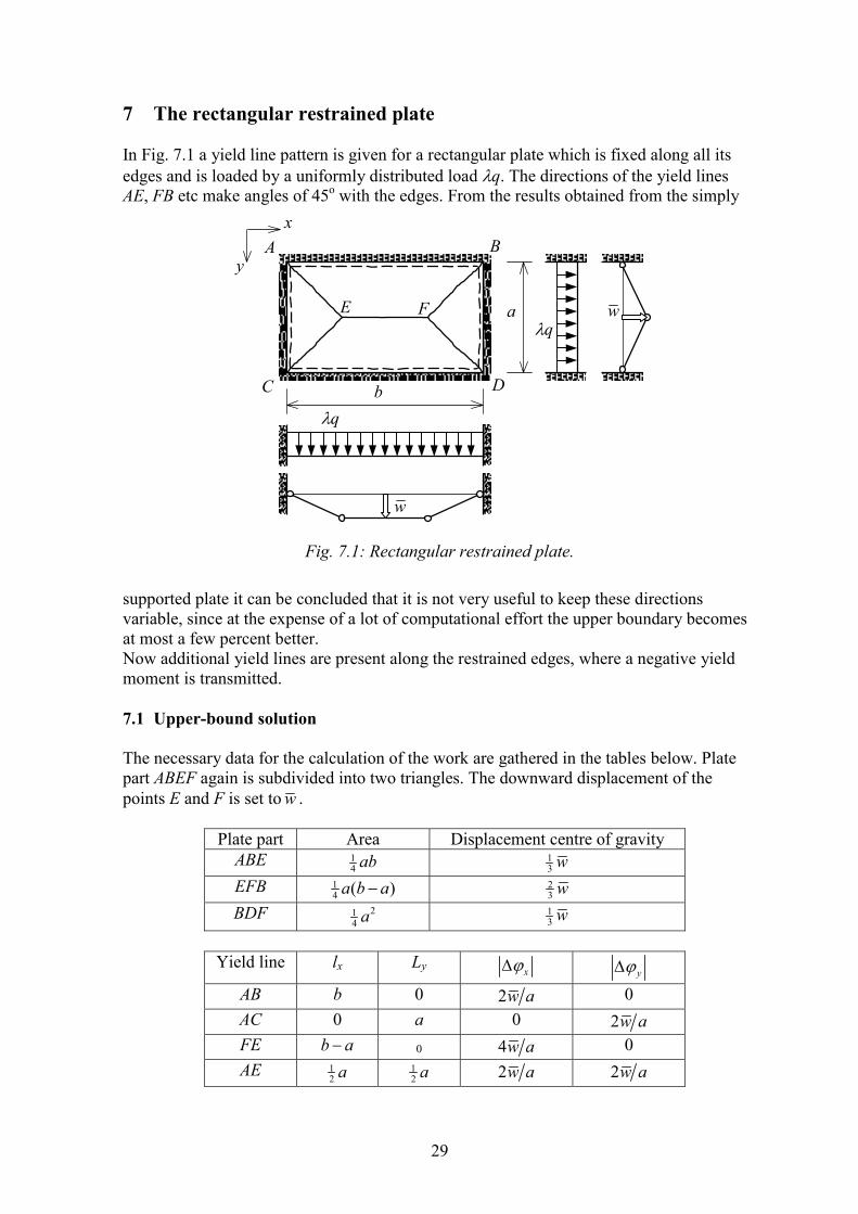
7 The rectangular restrained plate In Fig. 7.1 a yield line pattern is given for a rectangular plate which is fixed along all its edges and is loaded by a uniformly distributed load �q. The directions of the yield lines AE, FB etc make angles of 45o with the edges. From the results obtained from the simply

supported plate it can be concluded that it is not very useful to keep these directions variable, since at the expense of a lot of computational effort the upper boundary becomes at most a few percent better. Now additional yield lines are present along the restrained edges, where a negative yield moment is transmitted. 7.1 Upper-bound solution The necessary data for the calculation of the work are gathered in the tables below. Plate part ABEF again is subdivided into two triangles. The downward displacement of the points E and F is set to w .

Plate part Area Displacement centre of gravity ABE 1

4 ab 13 w

EFB 14 ( )a b a� 2

3 w BDF 21

4 a 13 w

Yield line lx Ly x�� y��

AB b 0 2w a 0 AC 0 a 0 2w a FE b a� 0 4w a 0 AE 1

2 a 12 a 2w a 2w a

Fig. 7.1: Rectangular restrained plate.

w

a

b �q

�q

C

A

F E

B

D

w

y

x

30

The external work and internal dissipation of the entire plate are:

1 1 ; 8 12 3 d p

bW qa b a w E m wa

�� � � �� � � � �� � � �� �

The upper bound then becomes:

2

16 1 where13

pm bqa a

�� �

�

� ��� �� �� ��� ��

(7.1)

This is exactly twice the result of the simply supported plate with corresponding mechanism and subjected to the same load (see (4.3) with � = 0.5). From the equilibrium method this is easy to comprehend. Consider the equilibrium of moments of part ABEF about line AB (see (6.2) and Fig. 7.2). The contribution mp�b of the

yield lines AE, EF and FB is exactly doubled by the clamping moment along AB. The contributions of �q and F remain the same. For plate part ADE a similar reasoning can be set up, which explains the doubling of �. 7.2 Lower-bound solution A lower-bound calculation is less fortunate. It seems obvious to double the contributions of mxx and myy by choosing a distribution similar to the one of the restrained beam:

1 8 1

1 8 1

xx p

yy p

x xm mb b

y ym ma a

� �� �� � � �� �� � �� �� �� � � �� �� � �

where the origin of the x-y co-ordinate system is put in A. However, for this choice of the bending moment distribution the case becomes twistless, because no freedom is left to chose torsional moments along the edges and in the middle of the plate. The load factor for this twistless lower-bound solution can be determined to be:

a

b

-2F

F F

A B

C

E F

Fig. 7.2: Equilibrium method applied to a restrained plate.

31

2 2

116 1 pmqa

��

� �� �� �� �

(7.2)

This result can be checked by considering the plate as a mesh of beams in x- and y- direction and to calculate �x and �y in these respective directions (see chapter 5).

For � = 1 only two third of the upper bound (7.1) is found. The main part of the difference can be attributed to the simplicity of the lower-bound approximation. But also the failure mechanism of Fig. 7.1 cannot be the real one. In order to explain this, the stress state of point A is considered. Both sections x = 0 and y = 0 transmit a bending moment of – mp. In section x = y a bending moment of + mp can be found. Using this data Mohr’s circle for point A can be constructed (see Fig. 7.3), from which it can be concluded that in the section x = – y the bending moment equals – 3mp, so the yield criterion is violated abundantly. The three yield lines AB, AE and AC cannot come together as indicated without violating the yield criterion in other directions. In reality, yield zones are created in the corners of the plate (Fig. 7.4a).

7.3 Approximation of yield zones The influence of such zones will be investigated by using an approximating pattern of yield lines according to Fig. 7.4b. In first instance a square plate will be analysed (� = 1), of which because of symmetry only a quarter needs to be considered. The geometry of the yield zone is fixed by two parameters �1 and �2. These parameters will be determined through a procedure of

mp-3mp

R 0y �

0x �

x y� �

-mp

x y�bending moments

torsional moments

R is direction centre

Fig. 7.3: Mohr's circle for point A.

C

A B

D C

A B

D a) b)

Fig. 7.4: Yield zone and approximation by yield lines.

32

optimisation. The work equation will be used to solve the problem. If the downward displacement of the plate centre D is indicated by w , the displacement of point G becomes: � �1 22 2Gw w� �� � The plate parts ECDG and FBDG (Fig. 7.5) are subdivided into triangles. For the calculation of |��x| and |��y| of the yield lines, initially the rotations �x and �y of all plate parts are determined.

Plate part Area Displacement of centre of gravity AEF 1

1 12 ( )( )a a� � 0 EFG 1 1

1 1 22 2( 2)( ) 2a a� � �� 11 23 (2 2 )w� ��

ECG & FBG 1 11 1 22 2( ) ( )a a� � �� � 1

1 23 (2 2 )w� �� CDG & BDG 1 1 1

1 22 2 2( )( )a a� �� � 11 23 (1 2 2 )w� �� �

Plate part �x �y

AEF 0 0 EFG 1 2 1 2(2 / )( ) ( 2 )w a � � � �� � 1 2 1 2(2 / )( ) ( 2 )w a � � � �� � � ECG 0 2 /w a� FBG 2 /w a 0 CDG 0 2 /w a� BDG 2 /w a 0

Yield line

lx ly |��x| |��y|

CE 0 112( )a�� 0 2 /w a

EF 1a� 1a� 1 2 1 2(2 / )( ) ( 2 )w a � � � �� � 1 2 1 2(2 / )( ) ( 2 )w a � � � �� �

FB 112( )a�� 0 2 /w a 0

EG 1 2( )a� �� 2a� 1 2 1 2(2 / )( ) ( 2 )w a � � � �� � 2 1 2(2 / )( ) ( 2 )w a � � �� FG 2a� 1 2( )a� �� 2 1 2(2 / )( ) ( 2 )w a � � �� 1 2 1 2(2 / )( ) ( 2 )w a � � � �� �

GD 11 22( )a� �� � 1

1 22( )a� �� � 2 /w a 2 /w a

From these data for the whole plate the external work, the dissipated energy and the load factor can be calculated to be:

C D w

A F

E

B y

x

G

H �1a

�2a 12 a

� �

1

11 22

lengths:

2

2

EF a

GH a

�

� �

�

� �

Fig. 7.5: Quarter of square restrained plate with approximated yield zone.

33

� �

� �

2 21 1 2

1 2

1 2

1 2

1 22 2

1 1 2

1 1 43

216 12

2148 21 4

d p

p

W qa w

E m w

mqa

� � � �

� �

� �

� �

� ��

� � �

� �� � �� �

� � � � �

��

� � ��

��� � �

��

The presence of the yield zones is expressed by the terms with �1 and �2. Compared to previous results, the magnitudes of both A and Ed have been reduced. However, it can be expected that the reductions are small. Before the optimum values of �1 and �2 will be determined the relation for the load factor is rewritten as (in analogy with 1/(1-x) � 1+x):

� �21 21 1 22

1 2

48 21 42

pmqa

� �� � � �

� �

� �� � � �� �

��

Equating the derivatives of this relation with respect to �1 and �2 to zero leads to:

� �

� �

2221 1 22

1 2

22112

1 2

4 12 8 02

2 4 02

�

� � �

� �

�

�

� �

� � � �

�

� � �

�

The second relation yields: �1 + �2 = 1/�2. With this result the first relation can be reduced to a quadratic equation in �1. Solution of this equation provides: 1 20.152 ; 0.277� �� � Substitution of these values in the initial equation for � gives:

2 2

48 440.880.96

p pm mqa qa

�� �

� �� �� �

which provides a reduction in � of about 10%. For the rectangular plate completely analogously it can be derived:

1 2

1 22

21 1 2

4116 21 8 ( )3 3

pmqa

� ��

� ��

� � � �

� �� �� ��

� ��� �� � �� ��

The optimum values for �1 and �2 are a bit different for this case, but the effect will be neglected. So, using the same values as for the square plate the load factor becomes:

34

2

16 0.760.36

pmqa

��

�

� �� �

��

A number of results obtained by this formula are listed in the last column of the table below. For the square plate a value is found of � = 44.0. Compared with the exact solution of � = 42.85 (found by Fox, [15]) it can be concluded that the upper-bound calculation applied on the mechanism of Fig. 7.5 leads to a very good result for a square plate and probably for rectangular plates too.

� Elastic �e Lower bound �p Upper bound �p 1.0 19.8 32.0 44.0 1.5 13.2 23.1 31.7 2.0 12.0 20.0 27.0 3.0 12.0 17.8 22.8 4.0 12.0 17.0 21.0 � 12.0 16.0 16.0

With: 20.3 ; 1pm qa� � �

The results of the previously discussed twistless lower-bound calculation are displayed in the third column. It has to be concluded that the lower-bound solution still falls far behind the corrected upper-bound solution. Finally, in the second column the load factors can be found leading to initial yielding of the plate. The first point of yielding is situated in the middle of the fixed long plate edge. Striking is the big difference between the load factors of initial yielding and total failure, which means that dimensioning with respect to the largest elastic moment is very uneconomical.

35

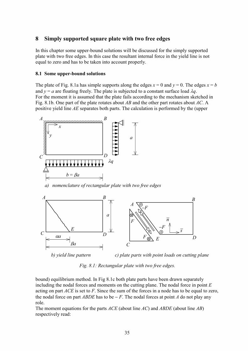
8 Simply supported square plate with two free edges In this chapter some upper-bound solutions will be discussed for the simply supported plate with two free edges. In this case the resultant internal force in the yield line is not equal to zero and has to be taken into account properly. 8.1 Some upper-bound solutions The plate of Fig. 8.1a has simple supports along the edges x = 0 and y = 0. The edges x = b and y = a are floating freely. The plate is subjected to a constant surface load �q. For the moment it is assumed that the plate fails according to the mechanism sketched in Fig. 8.1b. One part of the plate rotates about AB and the other part rotates about AC. A positive yield line AE separates both parts. The calculation is performed by the (upper

bound) equilibrium method. In Fig 8.1c both plate parts have been drawn separately including the nodal forces and moments on the cutting plane. The nodal force in point E acting on part ACE is set to F. Since the sum of the forces in a node has to be equal to zero, the nodal force on part ABDE has to be � F. The nodal forces at point A do not play any role. The moment equations for the parts ACE (about line AC) and ABDE (about line AB) respectively read:

n

F

Fig. 8.1: Rectangular plate with two free edges.

�a

a

b = �a

�q

a) nomenclature of rectangular plate with two free edges

y

x

C

A B

D

�a

a

C

A B

D E

b) yield line pattern c) plate parts with point loads on cutting plane

s�F

F

�F

C

A B

D E

36

� �

2

2 2

1 1 02 3

1 1 1 02 3 2

p

p

m a q a a F a

m a q a a q a a F a

� � � �

� � � � � �

� � � � � �

� � � � � � � � � �

From these relations F can be eliminated. Subsequently, the smallest value of � can be determined by differentiation with respect to �. Another possibility is to substitute directly the correct value of F. The load factor � then follows through elimination of �. This last method is applied here. In this case the real mechanism is not characterised by F = 0, because of the concentrated transverse force along the free edge (see chapter 5 and the third remark at the end of chapter 6). Also at the spot where the yield line intersects the free edge this transverse force may be present and then delivers a contribution to the nodal force.

For the determination of F the state of moments in point E is analysed with Mohr’s circle (Fig. 8.2). The three moments determining the circle are:

0 (boundary condition)

(properties of yield line)0

nn

nn p

ns

mm mm

�

� ��

� �

The angles � and �� in Fig. 8.2 are equal because they span up two identical circular arcs. For the torsional moment nsm it then follows: cotns pm m �� (8.1) where � is the angle between the n- and -n axis. Naturally, for a negative yield line a minus sign has to be added. In Fig. 8.1 the direction of F is chosen such that a positive F corresponds to a positive transverse force s nsQ m� Therefore: cotp pF m m� �� �

nnm

nsmn

s

n

s y

x

� � �

�

mp

mnn

direction of yield line

direction of free edge

bending moments

torsional moments

E

Fig. 8.2: Mohr’s circle at point E.

37

Substitution of the equilibrium equations leads after elimination of � to: 2 23 8 48 0� � �� � � where the value of qa2/mp is set to 1. Through elimination of � from the equilibrium equations a quadratic equation in � is found: 23 2 3 0�� � �� � �

2

p

qam�

1 2 3 4 5 6

2

6

4

0 �

5.55

1 2 3 4 5 6 �

�

0.00.20.40.60.81.0

0.72

a) b) Fig. 8.3: Relation between �, � and �.

2 26 (1 1 )

0pm qa� �

�

� �

�

2

1 2

5.500.68 ; 0.11

pm qa�

� �

�

� �

26 pm qa� �25.55 pm qa� �

C D

A B

�1a

a 0.72a

�a

a

�2a

C D

A B

C D

A B

C D

A B

a) b)

d) c)

Fig. 8.4: Yield patterns in plates with two simply supported and two free edges.

38

In Figs. 8.3a and 8.3b the values of � and � are plotted out versus �. Striking is the result � = 0.72 for the square plate. In first instance a symmetrical yield line pattern is expected with � = 1 (See Fig 8.4a). However, after some reflection the result appears not to be that strange: point D is stress free, which means no plastic yielding can occur. Otherwise it can be shown that the assumed failure mechanism is not correct as well. In point A the yield criterion appears to be violated slightly. On basis of this information the mechanism can be refined, for example as sketched in Fig. 8.4c. This however leads only to a very small reduction in load factor (1%). As competitive yield line pattern a mechanism can be chosen as indicated in Fig. 8.4d. It is for the reader to find out that the best mechanism can be found for � = 1 (boundary extreme). The corresponding load factor equals:

2 2

6 11pmqa

��

� �� �� �

� �

For all values of � this produces a load factor which is much higher than the load factor of the other mechanism. 8.2 Elastic solution The assumption seems to be lawful that for the plate a reasonable accurate upper bound has been found. This assumption is strengthened even more by the results of an elastic calculation by the finite element method. By this method applied on a square plate a load factor giving initial yielding is found to be:

24.93 pe

mqa

� �

It can be concluded that the elastic calculation provides a reasonable useful lower bound. The load path from initial yielding to full failure is quite short (this for example can be compared with the results of the constrained rectangular plate of chapter 7)

39

9 Circular plates From a practical point of view the application of circular plates is less important. However, the theoretical aspects are quite interesting. By making use of axial symmetry, the exact solution for a large number of problems comes within reach. This even holds for incremental elastic-plastic calculations and anisotropic material behaviour. In this chapter four classical cases will be discussed: Both the simply supported and restrained plate under a uniformly distributed load as well as a point load. Especially, the results of the point load are important, because they are quite useful for similar calculations on plates of arbitrary shape. 9.1 Uniform load on a simply supported circular plate As the first case a simply supported plate is considered, which is uniformly loaded by a surface load �q (Fig. 9.1). The plate still is assumed to be homogeneous and isotropic with plate yield moment mp. It is obvious to change to polar co-ordinates (r, �). The radius R of the plate is set to 0.5a.

Again the first step in the procedure is the choice of a proper yield line pattern. In the Figs. 9.2a, b and c yield line patterns are drawn for the regular triangle, square and hexagon, respectively. Continuation of this series leads to a pattern for the circle as shown in Fig. 9.2d. The number of drawn radial yield lines is arbitrary of course. Actually a yield zone covering the whole plate is present instead of a number of separate yield lines. Basically, the circle is approximated by a regular polygon. The simplest way to determine an upper bound for the failure load is to set up the equilibrium equation for a sector of the plate. Therefore, a plate part is considered between the lines � and � + d� (sector ABC in Fig. 9.3). From symmetry conditions it follows that

a

�q

R

� r

Fig. 9.1: Circular plate, simply supported and uniformly loaded.

a) b) c) d) Fig. 9.2: Yield line patterns for regular polygons.

40

along the edges AC and BC no torsional moments and transverse forces are acting. The equilibrium of moments for the yield line AB then becomes:

21 1 02 3pm Rd q R d R� � �� � � � �

For the upper bound for the failure load it now follows:

2 26 24p pm mqR qa

� � �

Comparison with the ultimate elastic solution (�e = 21.3 mp/qa2 for � = 0, see [10]) shows that the found upper bound is quite accurate. Later it will be shown that the value of � = 24 mp/qa2 is exactly equal to the real failure load. Note that the circular plate with a diameter a has exactly the same failure load as a square plate with side a (see chapter 4). Naturally, the problem can be solved by the work method too. A possible approach is to consider the plate as a regular n-polygon, after which the limit n � � is taken. However, here an alternative procedure is followed. To begin with, the linear bending deflection is presented in formula form:

1 ;rw w wR

� �� � �� �

� �downward displacement of centre point C

For the determination of the amount of dissipated energy the following points are important: �� both the torsional moments and the distortions are zero; �� the bending moments in radial directions do not contribute, because in the field of the

plate the radial curvatures are zero and along the edge r = R it holds mrr = 0; �� For the singular point in the middle of the plate it can be shown that it does not

contribute a finite amount to the dissipation (take w w� in an area r � R and let � 0). Thus, energy is dissipated only by the bending moments in tangential direction. Since there are no finite angular displacements the amount is equal to: d tt tt

plate

E m rdrd� �� ��

�

d�

Rd� R

C

A

B

Fig. 9.3: Circle sector ABC.

41

All tangential moments are equal to +mp. For axial symmetrical problems the tangential curvature is given by (see appendix, and [9] and [10]):

1tt

wr r

�

�� �

�

In this case /tt w Rr� � . The amount of dissipated energy then becomes:

2

0 0

2R

d p pwE m rdrd m wrR

�

� �� � � �� � (9.1)

The work performed by the external load equals:

2

2

0 0

11 26

R

plate

rW q w rdrd W q w rdrd qw RR

�

� � � � � �� � � �

� � � � � � � � �� � � �

�� � �

Equating the work and dissipation terms finally leads to the same the result as obtained by the equilibrium method. For the lower-bound calculation a parabolic moment distribution is assumed:

2

1 ;rr p tt prm m m mR

� �� �� � �� �

� �� � �

The torsional moments mrt are zero because of symmetry considerations. The moment distribution satisfies the boundary conditions and the yield criterion. Referring to the appendix and literature the equation for the equilibrium of moments is used for the determination of the transverse force:

2 2 2

2 31 1 p p p p prrr rr tt r r

m r m m r m m rmq m m q qr r r R r R r R

��� � � � � � � � � � �

�

Next, consider the equation for the equilibrium of vertical forces for the determination of the distributed load on the plate area:

1rr

qq qr r

��

� � ��

Substitution of the relation for qr leads to the conclusion that the given moment distribution is in equilibrium with a constant surface load �q, i.e.:

2 2 2

3 3 6p p pm m mq

R R R� � � �

�

� The uniformly distributed load �q can also be determined directly from the vertical equilibrium of a circle with radius r: �q(�r2) = � qr(2�r) = � 2qr/r.

42

Finally, it has to be checked whether a point load has been introduced in the centre of the plate as a result of singularities. From the fact that for r approaching zero the load qr goes to zero too, it can be concluded that this is not the case. Therefore, for the circular simply supported plate under a uniform load the real failure load has been found:

2 26 24p pp

m mqR qa

� � �

9.2 Uniform load on a restrained circular plate Fig. 9.4 shows the yield line pattern for this case. The difference with the previous problem is the yielding along the restrained edge.

Application of the equilibrium method for circle sector ABC shows that the presence of the restrained moment leads to a doubling of the amount of yield moments:

21 12 02 3pm Rd q R d R� � �� � � � �

So, the load factor is doubled as well:

2 212 48p pm mqR qa

� � �

Naturally, a work calculation has to lead to the same result. The dissipation term is built up out of the tangential moments given by (9.1) and a contribution of the restraining moment:

Fig. 9.4: Uniformly loaded restrained circular plate.

Rd�

A d� R

C

B

�q

w

a = 2R

43

2 2

0 0 0

2 2 4R

d p tt p p p pwE m rdrd m Rd m w m w m wr

� �

� � � � � ��

� � � � � � � � ��

� � �

This is exactly as expected because Ed doubles while W remains the same. Through a lower-bound calculation it can be shown that the calculated doubling of the load carrying capacity is realistic and does not need to be reduced as necessary with the rectangular plate. The assumed moment distribution for the lower-bound calculation is:

2

1 2 ;rr p tt prm m m mR

� �� �� � �� �

� �� � �

Further proof of this statement is left to the reader. 9.3 Point load in the centre of a simply supported circular plate The same yield line pattern as for the uniformly loaded plate is chosen (see Fig. 9.5). The amount of dissipated energy is still given by (9.1). The work by the external load �F does

not need any explanation. The work equation becomes: 2 2d p pW E Fw m w F m� � � �� � � � � (9.2) Note the size of the plate does not appear in the equations. The magnitude of the point load is determined by the plastic moment of the plate and not the diameter. No attention is paid here to the upper-bound calculation using the equilibrium method. This exercise is left to the reader. It is obvious to try out the following moment distribution for the lower-bound calculation: 0 ;rr tt pm m m� � These moments satisfy the yield criterion and the boundary conditions at position r = R. The transverse force can be derived from the moment distribution to be:

Fig. 9.5: Circular plate, simply supported and point loaded.

w

2c

�F �F

a

R

a) b) c)

44

1 1 prrr rr tt

mmq m mr r r r

�� � � � �

�

The distributed load follows from:

2

1 1 0p prr

m mqq qr r r r r

�� � � � � � �

�

This means that the field of the plate is not loaded. The transverse force qr however goes to �� for r � 0. In order to find out if this leads to a contribution of the load, the total transverse force Q has to be determined on a circular section at distance r from the centre point:

2 2

0 0

2r p pQ q rd m d m� �

� � �� � � � �� �

At each cut a force of Q = � 2mp is transmitted and therefore in the centre of the plate a point load �F = 2mp has to be present. This means that for the point load the exact solution has been found too. For the given moment distribution the relation mrr = mtt does not hold in the centre of the plate. This singularity is the result of the concentration of the load in one single point. In reality such a point load and resulting singularity do not occur. The load will always be distributed over a small area, for example over an area r � c with 0 � c � R as indicated in Fig. 9.5c. The upper bound in this case is given by:

2

213

pmF c

R

�� �

� (9.3)

It can be shown that this is the exact failure load too. For c � 0 the load approaches 2mp, while the moment distribution outside the loaded circle coincides more and more with the moment distribution of the point load. Please note that concentration of the entire load on smaller areas leads to an increase in vertical shear stress. For a given value of c punching will occur. The phenomenon of punching is not covered by this theory. 9.4 Point load in the centre of a restrained circular plate The mechanism of Fig. 9.6 is identical as the one of the uniformly loaded plate. The usual procedure is carried out:

2 2

0 0 0

2 2R

d p tt p p pwW E Fw m rdrd m rd F m w m wr

� �

� � � � � � ��� �

� � � � � � � �� ��

� � �

4 pF m� �� (9.4) This is the real failure load too, which can be proved through a lower-bound calculation on basis of the following moment distribution:

45

;rr p tt pm m m m� � � �

This moment distribution describes the yield zone in an optima forma manner. The whole plate is yielding in both principal directions: in radial direction with a negative and in tangential direction with a positive yield moment. Further Fig. 9.6c shows the case where the load is distributed over a small area. Through an upper-bound calculation it then follows:

4

213

pmF c

R

��

� (9.5)

Fig. 9.6: Circular plate, restrained edge and point loaded.

w

2c

�F �F

a

R

a) b) c)

r �

46

10 Point loads and simple supports on columns In this chapter a number of cases will be discussed of point loads and point supports. In practice the point support can be found mostly in the form of columns. The material behaviour is still isotropic and homogeneous as described in chapter 3. 10.1 Point load in the centre of a simply supported square plate For yield line AE in Fig.10.1 it holds:

1 ; 22x y x y

wl l aa

� �� � � � � �

Through the work equation it follows:

1 14 2 2 82 2d p p

w wW E Fw m a a F ma a

� �� �

� � � � � � � �� �

This also is the real failure load. The lower-bound solution found by Nielsen [12] for the domain �/4 � � � �/4 reads: 2tan ; 0 ;rr p rt tt pm m m m m�� � � � It is for the reader to make the proper derivations. In chapter 9 for the simply supported circular plate a higher load carrying capacity equal to �F = 2mp = 6.28mp was found (relation (9.2)). Probably an extra fixing effect is generated in the corners of the plate. For the square plate the failure load is independent of the plate size too. 10.2 Point load in the centre of a restrained square plate The mechanism according Fig. 10.2b leads to an upper-bound solution: 16 pF m� � The mechanism of Fig. 10.2c is the same that was used for the circular plate. The corresponding failure load is given by (9.4) and reads:

w

x

y � r

�F

a

C

A B

D

E

Fig. 10.1: Point load on simply supported square plate.

47

4 12.57p pF m m� �� � (10.1) The lower-bound solution of the circular plate is applicable too. Therefore, above relation represents the real failure load. Since the load carrying capacity is independent from the dimensions of the plate, relation (10.1) provides the exact point-load carrying capacity of all plates, which are completely restrained along the circumference. This failure load is valid too, when the point load is applied in an arbitrarily chosen point as shown in Fig. 10.2d or when the plate has an arbitrarily chosen shape. When the point load is applied on a limited area, then from (9.5) it can be concluded that the failure load is minimised for maximum radius R. In other words the yield circle which touches the plate edge determines the failure load. 10.3 Infinitely long simply supported plate For a given �, the failure load corresponding to the mechanism shown in Fig. 10.3 can be calculated from:

14 2pF m� ��

� �� �� �

� �

Fig. 10.2: Point load on restrained square plate.

w

�F

a �F

�F

�F

w wa) b) c) d)

w

w �F

�F �F a

a

a

x y n s

� R

� r

2�

�a �a C

A B

D

E

C

A B

D

E

Fig. 10.3: Point load on infinitely long simply supported rectangular plate.

48

The minimum is reached for � = 0.5�2, so that: 8 2 11.3p pF m m� � � The calculation for the mechanism of Fig. 10.3c requires some more explanation. The contributions of the yield zones AEC and BED can be determined by the formulae of the circular plate. The deflection for part BED equals:

1 21 11 for ; tan ;2 4

rw w R aR

� � � � ��

�� �� � � � � � � � ��

�

where w is the downward displacement of point E and (r,�) are polar co-ordinates. The tangential curvature is:

1 1tt

w w wr r r R rR

�

� � �� � � � � �� �

� �

The dissipated energy by the tangential moments in BED then holds:

0

2R

d p pwE m rdrd m wrR

�

�

� �

�

�

� �� �

The contribution of the radial moments along BD reads:

2 2d p pwE m R m wR

� �� �

Finally, yield line EB is considered. In the x-y co-ordinate system the rotations of part AEB are:

2 ; 0x ywa

� �� �

which can be transformed into the local n-s system by:

� � � �

� � � �

� �

� �

cos 2 sin 2 2 sinsin 2 cos 2 2 cos

xn

ys

w aw a

�� � � � ��

�� � � � ��

� �� � � �� �� �� �� � � �� �� � � � �� � � �� � � �

For the yield zone adjacent to yield line EB it holds that �s = 0 (At EB the n-direction coincides with the tangential direction). For the dissipation of yield line EB it then follows:

2cos 2d p pwE m R m wa

� �� � �

All contributions to the total dissipation are known now:

49

4 4 8d p p pE m w m w m w� � �� � � For the failure load it follows:

� � 1 18 8 tan2p pF m m� � � ��

�� �

� � � �� �� �

Minimisation of this failure load leads to � = 0.5 and therefore: � �4 2 10.3p pF m m� �� � � So, the mechanism of fig. 10.3c is representative. When a point load is applied in the neighbourhood of a simply supported edge and all other plate edges are more distant, then the mechanism of Fig. 10.3d develops, for which it holds: � � � �2 2 2 2 2 tanp p pFw m w m w m w� � � � � �� � � � � The first term of the right-hand side is originated from the tangential moments in the yield zone, the second term from the radial moments and the third term from the yield lines AE and EB. Division by w provides: � �2 2 2 2 tanp pF m m� � � �� � � The failure load is minimised for � = /4, i.e.: � �2 2 11.42p pF m m� �� � � 10.4 Point load on free edges and free corners In this section a point load on a free edge or corner will be discussed. Fig. 10.4 shows a number of cases for the straight edge and the square corner including the upper-bound value for �F. The straight edge and square corner can be considered as special cases of the free corner with aperture angle 2� (Fig. 10.5). On basis of the results displayed in Fig. 10.4 it is logical to make distinction between the two cases 2� � 90o and 2� � 90o. Fig. 10.5a shows the mechanism for 2� � 90o. Using an upper-bound calculation (work equation or direct equilibrium formulation) the corresponding failure load can be determined from: � �2 4pF m� � �� � � (10.2) Application of the mechanism of Fig. 10.5b for 2� � 90o provides: 2 tanpF m� �� (10.3)

50

Note that for the straight edge (2� = ) equation (10.2) corresponds to the mechanism of Fig.10.4c and that both (10.2) and (10.3) provide the same result of �F = 2mp for the square corner. The reader is advised to verify all presented results.

With a lower-bound calculation it now will be shown that both (10.2) and (10.3) provide the exact failure load. For the case of the plate with an obtuse angle it turns out that plate part BEC behaves as a part of a circular restrained plate, loaded by a point load. The total transverse force that can be transmitted by this plate part without violation of the yield criterion is equal to the product of the aperture angle and the maximum transmissible transverse force per radian:

� �4

2 42 2

pp

mm

��� � �

�

� �� � � �� �

�

This explains the last two terms of (10.2). Next, consider plate part ABE, in which the following moment distribution is present (choose the x-direction parallel to AE): ; 0xy yx p xx yym m m m m� � � � � For the principal directions (�, �) it holds:

d) pF m� �� e) 2 pF m� �

b) 0

0

6 ( 45 )

5.6 ( 35 )p

p

F m

F m

� �

� �

� �

� �

�F �F

�F �F

�F � �

a) 2 pF m� �� c) 0(2 ) ( 45 )pF m� � �� � �

Fig. 10.4: Point load on free edge and free right angle.

2�

C

A

B

D

E y

� x

� 45o2�

�F �F

a) b)

Fig. 10.5: Point load on free corner of aperture angle 2�.

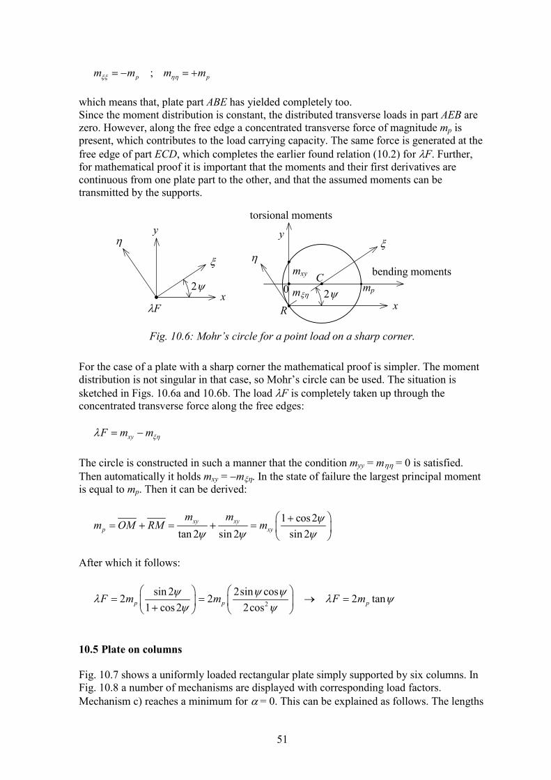
51

;p pm m m m�� ��� � � � which means that, plate part ABE has yielded completely too. Since the moment distribution is constant, the distributed transverse loads in part AEB are zero. However, along the free edge a concentrated transverse force of magnitude mp is present, which contributes to the load carrying capacity. The same force is generated at the free edge of part ECD, which completes the earlier found relation (10.2) for �F. Further, for mathematical proof it is important that the moments and their first derivatives are continuous from one plate part to the other, and that the assumed moments can be transmitted by the supports.

For the case of a plate with a sharp corner the mathematical proof is simpler. The moment distribution is not singular in that case, so Mohr’s circle can be used. The situation is sketched in Figs. 10.6a and 10.6b. The load �F is completely taken up through the concentrated transverse force along the free edges: xyF m m��� � � The circle is constructed in such a manner that the condition myy = m�� = 0 is satisfied. Then automatically it holds mxy = �m��. In the state of failure the largest principal moment is equal to mp. Then it can be derived:

1 cos2tan 2 sin 2 sin 2

xy xyp xy

m mm OM RM m �

� � �

� ��� � � � � � �

� �

After which it follows:

2

sin 2 2sin cos2 2 2 tan1 cos2 2cosp p pF m m F m� � �

� � �� �

� � � �� � � �� � � �

�� �

10.5 Plate on columns Fig. 10.7 shows a uniformly loaded rectangular plate simply supported by six columns. In Fig. 10.8 a number of mechanisms are displayed with corresponding load factors. Mechanism c) reaches a minimum for � = 0. This can be explained as follows. The lengths

2�

y �

x

� mxy

m�� mp 0

R

bending moments

torsional moments

C

y

�

x

�

2�

�F

Fig. 10.6: Mohr’s circle for a point load on a sharp corner.

52

of the yield lines are proportional to �. For a given downward displacement of the centre of the plate, the angles of rotation are just inversely proportionate to �. Therefore, the internal virtual work is independent of �. Since the work performed by the load increases for decreasing � the lowest load factor is found for � = 0. The interpretation of this mechanism is that the reactions in the supports have reached their maximum capacity. In other words the plate is not capable of transmitting higher concentrated support forces, analogously to the situation with point loads as discussed in the previous section. This can be verified by using the results of Fig. 10.4b and 10.4e. This interpretation then automatically leads to mechanism d). Naturally, the corresponding load factor can be determined by the developed standard techniques. However, the results found in previous section can be used directly too. From Fig. 10.4e it can be concluded that the support reactions in the corners A, B, C and D can increase to a value of 2mp. The maximum reaction forces in E and F are (2 + )mp (Fig. 10.4c). Summation of all these maximum reaction forces provides an upper bound for the total load of:

54 a 5

4 a

a

C

A B

D

E

�q

F

Fig. 10.7: Plate supported by six columns.

�a

�a

a) 28 pm qa� �

c) 2

minimised for 08 pm qa

�

�

�

�

b) 54

2

minimised for ( 2 1)

7.45 pm qa

�

�

� �

�

�a

C

A B

D

E

F d) 27.31 pm qa� �

Fig. 10.8: Different yield line patterns.

53

� � � �22 2

5 44 2 2 2 6 7.312 5

p pp p

m mqa m m

qa qa� � � �� � � � � � � � �

Comparison of the four discussed mechanisms shows that mechanism d) is the most dangerous one. Again it should be noted that exceeding of the maximum allowable vertical shear stress is not noted by this theory (punch mechanism).

54

11 Yield criteria of the largest principal moment, Tresca and von Mises In this chapter the most well known yield criteria will be discussed. Firstly a general formulation will be given. After that attention will be paid to the square, Tresca and von Mises yield criteria. 11.1 General formulation of yield criteria For the description of elastic-ideal-plastic material behaviour usually a so-called yield function � is used in combination with a material constant K. The relation for � is a function of the relevant stress parameters s2, s2, � sn. Further, � and K have the following properties (some nomenclature for two stress components is indicated in Fig. 11.1): 1. Combinations of the stress parameters for which � (s2, s2, � sn) < K are “safe”

combinations. The material responds elastically to variations of the stresses. 2. When somewhere for certain stress combinations it holds � (s2, s2, � sn) = K, then the

material may yield at that spot. Changes in the stress state can occur only, if the relation �� � 0 is satisfied. The total set of stress combinations with � = K AND � < K are called “permissible” combinations.

3. Stress combinations leading to � > K are physically impossible.

Sometimes more yield functions � k are required for the description of a yield criterion. A “safe” stress combination has to satisfy all conditions � k < Kk. The material may flow if for one of the conditions it holds: � k = Kk. Note that this formulation of yielding shows a lot of similarities with the description of the failure mechanism for frames. In that case � is a function of the relevant load parameters and the material constant K is equal to the yield moment mp (see “Vloeifunctie en normaliteitsconditie (translation: Yield function and normality condition), annex to the course b19a of Prof. ir J. Witteveen). 11.2 The yield criterion of the largest principal moment (square yield criterion) Up to now this handbook silently used the yield criterion of the largest (absolute) principal moment, normally indicated as the square yield criterion. Using the yield function this criterion can be formulated as (also see Fig. 11.2a): � �max , ;I II pm m K m� � � (11.1)

s1

s2 � > K

� < K � = K

Fig. 11.1: General yield criterion for two stress components (yield contour).

0

55

Through the relations (5.5) the yield criterion can be expressed in the bending and torsional moments with respect to the x-y co-ordinate system:

� � � �2 21 1max ;

2 4xx yy xx yy xy pm m m m m K m�

� �� � � � � �� �

� �

(11.2)

Yield criterion (11.2) is displayed in Fig. 11.2b. Along the axes mxx, myy and mxy are plotted out. Only the part has been drawn for which mxy � 0. The part for which mxy < 0 can be obtained by reflection with respect to the plane mxy = 0. For mxy = 0 the moments mxx and myy become principal moments and the intersection of the three-dimensional yield surface with the plane mxy = 0 again produces Fig. 11.2a. Intersection with the planes mxx = 0 and myy = 0 provide parabolas indicated by the dashed lines. The intersection for which mxx = �myy produces an ellipse and finally the intersection for which mxx = +myy gives a triangle. For better understanding the reader is advised to draw a number of special points on the yield surface with the aid of Mohr’s circle. Fig. 11.2c shows another property of the yield figure. It is possible to compose the yield surface out of two elliptical cones. The base of both cones is formed by the ellips in the plane mxx = �myy. The apexes of the cones are situated in the plane mxy = 0 at positions mxx = myy = � mp. Another view on the yield surface can be obtained by reformulating relation for the yield surface as follows:

b) with respect to x-y moments (eq. (11.2))

mxx

mxy

myy

mxx = myy

mxx = � myy

mxy

mxx

myy

mp

mp

� mp

� mp mI

mII

� mp

mp

mp � mp

mxx = � myy

mxx = myy

mxx

myy

Fig. 11.2: Square yield criterion.

a) with respect to principal moments (eq. (11.1))

c) with respect to x-y moments (eq. (11.2)) d) contour plot for mxy (eq. (11.3))

56

� �� �

� �� �

2)

2)

xy p xx p yy

xy p xx p yy

m m m m m

m m m m m

� � �

� � �

(11.3)

These formulae can be derived algebraically from (11.2) using Mohr’s circle with � = K. Looking at (11.3) it is quite obvious to draw contour lines for mxy is constant (see Fig. 11.2d). The contour lines are hyperbolas with the lines mxx = � mp and myy = � mp as asymptotes. It easily can be checked that the two sets of hyperbolas intersect at the line mxx = �myy. In the shaded part the first relation of (11.3) is valid. Combinations of mxx, myy and mxy deliver a positive principal moment mp. In the unshaded part the second relation is valid and the principal moment mp is negative.

All in all, the yield criterion of Fig. 11.2 is quite complicated. Therefore, often use is made of the pyramid shaped approximation as drawn in Fig. 11.3a. Common points with the exact yield criterion are the lines in the plane mxy = 0, the intersection mxx = myy and the top mxy = mp. The formula reads: � �max , ;xx xy yy xy pm m m m K m� � � � � (11.4)

Since the original yield criterion is convex, the linearised criterion (11.4) is a safe approximation. The derivation of this approximation is often carried out through Mohr’s circle as shown in Fig.11.3b. 11.3 The yield criterion of Tresca Tresca’s yield criterion is based on the largest shear stress in the three dimensional stress space. If I, II and III are the three principal stresses, the yield criterion of Tresca can be written as (see Mohr’s circle in Fig. 11.4a): � �max , , ;I II I III II III pK� � � � � � � �� � � � � (11.5) For a plane stress situation where III = 0 it follows (see Fig. 11.4b):

mxx

mxy

myy

mxx = myy

mxx = � myy

mp

mp

mxx + mxy

mI

mxx

myy

mxy

myx

torsional moments

bending moments

a) b) Fig. 11.3: Approximated square yield criterion.

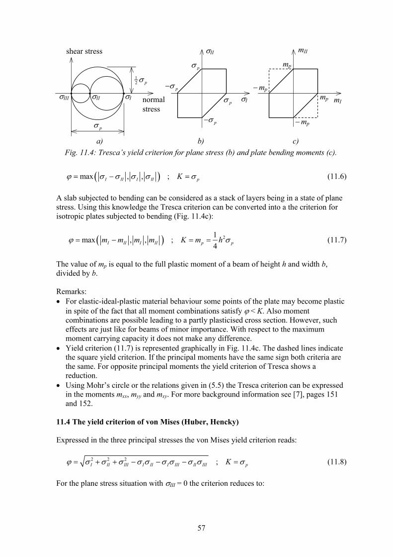
57

� �max , , ;I II I II pK� � � � � �� � � (11.6) A slab subjected to bending can be considered as a stack of layers being in a state of plane stress. Using this knowledge the Tresca criterion can be converted into a the criterion for isotropic plates subjected to bending (Fig. 11.4c):

� � 21max , , ;4I II I II p pm m m m K m h� �� � � � (11.7)

The value of mp is equal to the full plastic moment of a beam of height h and width b, divided by b. Remarks: �� For elastic-ideal-plastic material behaviour some points of the plate may become plastic

in spite of the fact that all moment combinations satisfy � < K. Also moment combinations are possible leading to a partly plasticised cross section. However, such effects are just like for beams of minor importance. With respect to the maximum moment carrying capacity it does not make any difference.

�� Yield criterion (11.7) is represented graphically in Fig. 11.4c. The dashed lines indicate the square yield criterion. If the principal moments have the same sign both criteria are the same. For opposite principal moments the yield criterion of Tresca shows a reduction.

�� Using Mohr’s circle or the relations given in (5.5) the Tresca criterion can be expressed in the moments mxx, myy and mxy. For more background information see [7], pages 151 and 152.

11.4 The yield criterion of von Mises (Huber, Hencky) Expressed in the three principal stresses the von Mises yield criterion reads: 2 2 2 ;I II III I II I III II III pK� � � � � � � � � � �� � � � � � � (11.8) For the plane stress situation with III = 0 the criterion reduces to:

II

p��

p��

p�

p�

p�

normal stress

shear stress

12 p�

I

II

III I mI

mII

mp

mp

� mp

� mp

a) b) c) Fig. 11.4: Tresca’s yield criterion for plane stress (b) and plate bending moments (c).

58

2 2 ;I II I II pK� � � � � �� � � � (11.9) Analogous to the reasoning held for the Tresca criterion, the von Mises yield criterion for plate moments becomes:

2 2 21;4I II I II p pm m m m K m h� �� � � � � (11.10)

Naturally, this criterion can be expressed in the moments mxx, myy and mxy too.

The three yield criteria discussed are displayed together in Fig. 11.5. Note that all three criteria can be used only for the description of the yield behaviour of isotropic materials. Tresca and von Mises are used in most cases for the description of steel and aluminium, where von Mises compares a bit better with experimental results. For a specific case the choice is made mostly on basis of the applied mathematical techniques. The square criterion can be used for the analysis of “isotropic” reinforced concrete slabs having two mutually perpendicular and equal reinforcements, both at the top and bottom. As such, it is a special case of the general yield criterion for reinforced concrete that will be discussed thoroughly in the chapter. The presented formulae will be used in a lower-bound calculation of a torsion panel. In fact, the upper-bound calculation using the square criterion has already been given in section 10.4 (“Point load on free edges and free corners”). The upper-bound calculations using the yield criteria of Tresca and von Mises will be discussed in chapter 13, because an extra addition on the material behaviour is required (flow rule). 11.5 Lower-bound calculation of a torsion panel A square plate ABCD has simple supports at the corners A, B and C. In point D a point load is acting of magnitude �F (load case of Nadai, see [9], [10] and [13]). The moment distribution given by:

10 ; ; 02xx xy yx yym m m F m�� � � � �

von Mises Tresca square

mp

mp

� mp

� mp

mI

mII

Fig. 11.5: Several yield criteria.

59

satisfies all equilibrium conditions. The principal moments in each point of the plate read:

1 1;2 2I IIm m F m m F�� ��� �� � � � � �

Both principal moments have the same magnitude but opposite signs. For the three yield criteria it is found:

mI mII �F Square criterion

pm� pm� 2.00 pm Tresca criterion 2pm� 2pm� 1.00 pm von Mises Criterion 3pm� 3pm� 1.15 pm

From the corresponding upper-bound calculations (chapters 10 and 13) it can be concluded that for all three cases the exact failure load has been found. It can be observed that the influence of the type of yield criterion on the maximum load carrying capacity of the torsion panel is large.

mp

mp

� mp

� mp

mI

mII

mI

mII ( , )3 3p pm m

�

1 12 2( , )p pm m�

mI

mII

C

A B

D

a � �

�F

Fig. 11.6: Torsion panel.

60

12 Yield criterion for reinforced concrete slabs In this chapter the yield criterion will be derived for a reinforced concrete slab with both upper and lower reinforcement in x- and y-direction, where the upper and lower reinforcement percentages may be different. So, the properties of the plate are orthogonal-

anisotropic, also called orthotropic. Figs. 12.1a and 12.1b show the reinforcements of the slab. The percentage of lower reinforcement in x-directions is indicated by �x and the percentage of upper reinforcement in x-direction by ��x. For the reinforcements in y-direction similar notations are used. 12.1 Yield line in x- or y-direction As a start, the case is considered where a positive yield line cuts the slab parallel to the y-direction (Fig. 12.1c). When extension forces are not taken into account, a plate bending moment mxx of magnitude mpx will be present in the yield line. The stress distribution in the same cross section is given in Fig. 12.1d, where it has been assumed that the concrete does not sustain tensile stresses. Thus the tensile force in the cross section is equal to the yield force �x ph of the reinforcement. This tensile force is in equilibrium with the compressive force ca. The compressive force is solely transmitted by the compressive stresses in the concrete c, since the eventual influence of the upper reinforcement can be neglected. The equilibrium of moments in the section provides:

� �21 or 12px x p px x p xm h h a m h� � � � �

� ��� � � �� �

�

x�

y� �

x� �

pb�

x

y

x

y

x

y

mxx = mpx

h h� a

�xh p ps�

p�

y�

c

a) b)

c) d) e)

Fig. 12.1: Scheme of orthotropic reinforced concrete slab.

61

where �x is a coefficient depending on the concrete cover of the lower reinforcement in x-direction, the concrete compressive strength c and the percentage of reinforcement �x. For all moments it thus can be written:

� �

� �� �

� �

2

2

2

2

1

1

1

1

px x p x

py y p y

px x p x

py y p y

m h

m h

m h

m h

� � �

� � �

� � �

� � �

� �

� �

� � �� �

� � �� �

(12.1)

In this respect take note of the following remarks: �� In a yield line a certain amount of rotation capacity has to be present. This creates

demands on the maximum reinforcement percentage (see handbook of the basic course b19A).

�� The assumed stress distribution in the cross section (Fig. 12.1d) completely satisfies the conditions of the laws of plasticity. This stress distribution is compatible with a kinematical allowable plastic strain distribution across the section (Fig. 12.1e)(see handbook of the basic course b19A).

12.2 Yield line under an angle with the y direction Now the case is considered that a positive yield line cuts the slab under angle � with the y-axis. The moments mnn and mns in the yield line have to be determined. The lower reinforcement now extends in both directions. It is assumed that the concrete at the lower side does not contribute to the stress transmission in the yield crack. The moments transmitted in the yield line from one plate part to the other are partly generated by the reinforcement in x-direction and partly from the reinforcement in y-direction. When considering a small piece of yield line of length ds, the reinforcements in x- and y-directions deliver vectorial moments dMy and dMx, respectively of magnitudes (see Fig.

a) b) c)

sinx pydM m ds �� �cosy pxdM m ds ��

x

y

ds cos� ds cos� ds sin� ds sin�

ds ds

dMn = � mnsds dMs = mnnds

ds

mpxdy mpydx �

n s

mns mnn

d) e) f) Fig. 12.2: The internal moments of a positive yield line.

62

12.2b, e, c and f ; and take note of the subscripts): cos ; siny px px x py pydM m dy m ds dM m dx m ds� �� � � � � � (12.2) Decomposition of these moments with respect to the n-s co-ordinate system provides (Fig. 12.2d): cos sin ; sin cosn ns x y s nn x ydM m ds dM dM dM m ds dM dM� � � �� � � � � � � � Combination with (12.2) yields:

� �

2 2cos sin

sin cosnn px py

ns py px

m m m

m m m

� �

� �

� �

� �

(positive yield line) (12.3)

On basis of (12.3) it can be concluded that a yield line generally transmits a torsional moment. The torsional moment is zero only if the plastic moments mpx and mpy are equal to each other or if yielding occurs in one of the reinforcement directions (sin� = 0 or cos� = 0). In all other cases the torsional moment is not equal to zero. In the normal upper-bound calculation this has no consequences because the torsional moment does not produce any work. However, the alternative upper-bound calculation of chapter 8 indeed is affected by the presence of a torsional moment. Then the real failure mechanism is no longer characterised by the disappearance of the nodal forces. Finally it is remarked that the bending moment in the yield line is independent of the direction and is equal to mp , i.e. mpx = mpy = mp. Above relations are valid for a positive yield line. Completely analogously similar formulae can be derived for a negative yield line. The result becomes:

� �

2 2cos sin

sin cosnn px py

ns px py

m m m

m m m

� �

� �

� �� � �

� �� �

(negative yield line) (12.4)

On basis of (12.3) and (12.4) upper-bound calculations can be performed for yield line mechanisms. For a yield line of length ls and plastic rotation ��s the dissipated energy according to (3.4) equals:

0

sl

d nn sE m ds�� �� ��

For a positive yield line this can be worked out as follows:

� �2 2cos sin

cos cos sin sind px py s s

d px s s py s s

E m m l

E m l m l

� � �

� � � � � �

� � � �

� � � �

This leads to the following simple result, which could have been obtained without derivation too:

63

d px y y py x xE m l m l� �� � � � (positive yield line) (12.5) For the negative yield line a similar result can be derived: d px y y py x xE m l m l� �� �� � � � (negative yield line) (12.6) Note that the derived formulae (12.3), (12.4), (12.5) and (12.6) for the case mpx = mpy = mpx = mpy are in complete agreement with the square yield criterion. This also proves the previously postulated proposition that the square yield criterion can be used for a reinforced concrete slab with identical upper and lower reinforcements in both x- and y-directions (isotropic). As an illustration an upper-bound calculation will be carried out on the earlier introduced torsion panel. 12.3 Yield line calculation of reinforced concrete torsion panel Fig. 12.3 shows two different yield line patterns. The mechanism of a) has a negative yield line. Using (12.6) it is found:

d px pyw wE m b m bb b

��

� �� � � � � �

The work done by the external load equals: W F w�� � From which it follows: � � � �1px pyF m m� � �� �� � This relation is minimised for px pym m� � �� , the lowest upper bound then becomes:

C D

A

F

E

B

C D

A

G

H

B

�b �b

�F �F w w

x

y

abb

a) b) Fig. 12.3: Yield-line pattern of torsion panel.

64

2 px pyF m m� � �� � (negative yield line) (12.7) Analogous a positive yield line with minimising factor px pym m� � provides: 2 px pyF m m� � � (positive yield line) (12.8) Of course, the lowest value of both mechanisms is decisive. In the special case with mpx = mpy = mpx = mpy = mp for both mechanisms it follows (minimising factor � = 1): 2 pF m� � This result indeed corresponds with the found value for the square yield criterion (section 10.4: Point load on free edges and free corners, see Fig. 10.4e). 12.4 Yield criterion formulated in moments with respect to the x-y system For the sake of lower-bound calculations and design procedures it is required to reformulate the yield criterion for reinforced concrete in moments with respect to the x-y co-ordinate system. Therefore, Fig. 12.4 is considered where a positive yield line has been

drawn under an angle � with the y-axis. Along the cathetusses the plate moments mxx, myy and mxy are acting. On the hypotenuse the two vectorial moments dMx and dMy are present, which already have been derived in Fig. 12.2 (relation (12.2)). Two moment equilibrium equations for the triangular plate part can be se up: ;xx yx y xy yy xm dy m dx dM m dy m dx dM� � � � � Using dx = ds sin�, dy = ds cos� and the relations for dMy and dMx given by (12.2) it can be derived: cos sin cos ; cos sin sinxx yx px xy yy pym m m m m m� � � � � �� � � � (12.9)

sinx pydM m ds �� �

cosy pxdM m ds �� ds cos�

ds sin�

ds

x

y

myx

myy

mxy

mxx �

Fig. 12.4: Arbitrary stress state mxx, myy and mxy causing a positive yield line.

65

Division of both relations by cos� and introduction of tan� provides the following formulae�:

tan ; tanpx xx xy

yx py yy

m m mm m m

� �

�

� �

�

(12.10)

Elimination of tan� finally gives: � �� �2

xy px xx py yym m m m m� � � (positive yield line) (12.11) Similarly for a negative yield line it follows: � �� �2

xy px xx py yym m m m m� � �� � (negative yield line) (12.12) The surface described by (12.11) and (12.12) is based on a mechanism and provides an upper bound for the real failure behaviour. However, it can be shown (chapter 13) that (12.11) and (12.12) actually describe the real yield surface. Combinations of mxx, mxy and myy are therefore “safe” if the following condition is satisfied:

� �� �

� �� �2 min

px xx py yy

xy

px xx py yy

m m m mm

m m m m

� � ��� �

� �� ���

(12.13)

For completeness it is required that mxx � mpx, �mxx � m�px etc. In Fig. 12.5 both (12.11) and (12.12) are drawn as contours for mxy. Combinations of mxx, myy and mxy in the shaded area produce a positive yield line (eq. (12.11)), while combinations in the unshaded part produce a negative yield line (eq. (12.12)).

� Sometimes it is thought that these relations provide the principal directions of the moments. This is NOT true. The angle � is the direction of the yield line in which normally a torsional moment is present.

pym��

pxm��

mpy

mpx

mxx

myy myy

mxy

from upper reinforcement

from lower reinforcement

Fig. 12.5: Yield criterion for orthotropic reinforced concrete (contours for mxy).

66

Note the correspondence with the square yield criterion (see (11.3)). When the two contour plots are compared (Figs. 12.5 and 11.2d), then it can be seen that in both cases the contour lines consist of two sets of hyperbola, intersecting each other on the descending diagonal of the ground plane (check this!). For orthotropic reinforced concrete the ground plane is no longer a square but a rectangle with a shifted origin. For orthogonal isotropic reinforced concrete (At the top and bottom side in both directions identical reinforcements) the yield criterion coincides exactly with the square yield criterion.

Similarly to the square yield criterion, the yield criterion can be represented by two elliptical cones (Fig. 12.6). Basically, the cones of both criteria are identical (type: z2 = xy), only the positions of the apexes in the ground plane are different. From both Figs. 12.5 and 12.6 it can be seen that mxy reaches its maximum at the intersection of both diagonals, i.e. for the following combination:

� � � �1 1;2 2xx px px yy py pym m m m m m� � � �� � (12.14)

So, the largest value does not occur for mxx = myy = 0. After substitution of these moments into (12.11) or (12.12) for the maximum value of mxy it follows:

� �� �max

12xy px px py pym m m m m� � �� � (12.15)

On basis of this result, the yield surface for reinforced concrete can be approximated by formulae that are similar to (11.4). The approximation again is a pyramid (Fig.12.7), but now with rectangular base in the mxx-myy plane and apex given by (12.14) and (12.15). On basis of the convexity of the yield surface it can be concluded that this approximation is at the safe side. In order to obtain the equation for lateral face a in Fig. 12.7, it is sufficient to determine the intersection with the mxx-mxy plane. The equation of the intersecting line can easily derived to be:

� �max

1

12

xyxx

pxpxxy

px px

mmmm m

m m

� �

� �

Substitution of (12.15) after some derivations leads to:

Fig. 12.6: Yield criterion for orthotropic reinforced concrete (intersecting cones; negative values for mxy can be obtained by reflection with respect to base).

pxm��

pym��

mxy

mxx

myy

mpx

67

px pxxx xy px

py py

m mm m m

m m� �

� �� �

For the other lateral faces similar results can be derived. Further, four more faces for negative mxy exist. This finally leads to the following set of inequalities to be satisfied by combinations of mxx, myy and mxy:

1

1

xx xy px

xx xy px

yy xy py

yy xy py

m m m

m m m

m m m

m m m

�

�

�

�

� � �

� � � �

� � �

� � � �

� � � �with px px py pym m m m� � � �� � (12.16)

Above set of equations is not applied frequently in practice. The practical approximation commonly used reads:

xx xy px

xx xy px

yy xy py

yy xy py

m m m

m m m

m m m

m m m

� � �

� � � �

� � �

� � � �

(12.17)

where the left-hand sides are called the reinforcement moments. These formulae already have been given in chapter 5 (see (5.7)). Now it will be shown that this set is a safe approximation for the yield criterion. Therefore, the graphical representation of (12.17) in

maxxym

� �12 px pxm m��

� � max12

pxxy

px px

mm

m m��

pym��

pxm��

pxm��

mxy

myy

mxy

mxx

mxx

myy

a b

c

d

mpy

mpx

mpx

Fig. 12.7: Yield criterion for orthotropic reinforced concrete (approximation by (12.16)).

68

Fig.12.8 is considered. Because of the convexity of the yield surface it is sufficient to show that the points E and F are permissible points. Proof will be given for point E, for point F proof is identical. The “co-ordinates” of point E are given by:

� � � � � �1 1 1; ;2 2 2xx px py py yy py py xy py pym m m m m m m m m m� � � � � � � �� � � �

Remark: Silently all the time it is assumed that mpx+ m�px > mpy+ m�py. The other case is possible as well and proof can be given in a similar way. Point E is situated below the descending diagonal AD, which means it is controlled by the top reinforcement. Therefore, the second relation of (12.13) has to be satisfied, leading to:

Fig. 12.8: Yield criterion for orthotropic reinforced concrete (approximation by (12.17)).

� �12 py pym m��

pym��

pxm��

pxm��

mxy

myy

mxy

mxx

mxx

myy

A B

C D

mpy

mpx

E F

� �12 py pym m��

E F

Fig. 12.9: Yield criterion for orthotropic reinforced concrete (exact by (12.13) and approximations by (12.16) and (12.17)).

pym��

pxm��

mpy

mpx

mxx

myy myy

mxy

mxx

mxy

B

B

section A-A

Section B-B

A A

(12.17) (12.13) (12.16)

(12.13) (12.16)

(12.17)

69

� � � � � �?21 1 1

4 2 2py py px px py py py py pym m m m m m m m m� � � �� � � � � � �� � � � � �� � � �

Since both left-hand side and right-hand side are equal, points E and F are situated exactly on the yield surface. This proves the safe character of the approximation. It also should be mentioned that not only the points E and F are situated on the yield surface, but the entire edges CE and FB. Since these lines are generating lines of the two cone surfaces. Finally, Fig. 12.9 is considered where the exact yield surface and the two approximations have been drawn for comparison. It can be seen that the approximations both perform well and badly in different areas. The first approximation performs well for high values of the torsional moment, while the second approximation performs better for small values of mxy. This will be confirmed by the lower-bound calculation of next example. 12.5 Example: lower-bound calculation of reinforced concrete torsion panel For the torsion panel (Fig. 12.10a) the same moment distribution is chosen as for the lower-bound calculations already carried out with the Tresca and von Mises criterion:

10 ;2xx yy xym m m F�� � �

On basis of the exact formulae (12.13) for the yield criterion of reinforced concrete the following inequalities have to be satisfied:

� �� �

� �� �� �

2 0 01 min 2min ,2 0 0

px py

px py px py

px py

m mF F m m m m

m m� �

� � ��� � � � � � � � � � � � ��

14 pm�

14 pm�

14 pm�

14 pm�

14 pm�

14 pm

14 pm

mxx

mxx

mxx

mp myy

myy

myy

mp

�mp

mp

mp x

y

�F

a) b)

c) d)

Fig. 12.10: Torsion panel with different reinforcement schemes.

70

From comparison with the results of the upper-bound calculation on the same problem (see (12.7) and (12.8)) it can be concluded that the exact solution has been found. Assuming that the panel has heavy reinforcements in x-direction (mpx = m�px = mp) and light reinforcements in y-direction (mpy = m�py = mp/4), then the exact failure load is equal to:

1 12min ,4 4p p p p p pF m m m m m�

� �� � � �� �� �

� �

Next the approximation according to (12.16) is considered. Substitution of the moment distribution leads to:

� � � �1 12min , , , withpx px py py px px py pyF m m m m m m m m� � � �� �

� �� � � �� � � �� �

For the considered reinforcement scheme it follows:

� �

1 1 24 4

1 1 1 12min , ,2 , 22 2 4 4

p p p p

p p p p p

m m m m

F m m m m m

�

�

� �� � � �� �

� �

� � �� �

� �

which is identical to the exact solution. This result could be expected since the point mxx = myy = 0 of the used yield criterion is situated exactly on the intersection point of the diagonals, where the apex of he pyramid coincides with the real yield surface (see Fig. 12.10b). Considering the nature of the second approximated yield criterion given by (12.17) the results obtained are not that good. Substitution of the moment distribution yields:

1 1 12min , , ,4 4 2p p p p pF m m m m m�

� �� �� �

� �

Indeed, the load carrying capacity is underestimated by a factor two. It completely depends on the circumstances, which of the two approximations provides the best results. For the case given in Fig. 12.10c the tables are turned and the second approximation gives the exact solution. For the yield figure given in Fig. 12.10d both approximations coincide, and on top of that deliver the exact answer. Further the accuracy of the approximations depend on the ratio of the moments mxx, mxy and myy. If mxy = 0, naturally both approximations produce exact answers. Some concluding remarks �� Fig. 12.10d represents a concrete slab with a lower reinforcement, which is identical in

two mutually perpendicular directions. It has a similar upper reinforcement, however with a different percentage of reinforcement (mpx = mpy = mp; m�px = m�py = m�p). Such a reinforced slab behaves like a quasi isotropic plate, which easily can be seen from the relations (12.3) and (12.4) - the bending moments in the yield line respectively are mp and m�p, and the torsional moment in the yield line is zero -. Upper-bound calculations of slabs with this type of reinforcements are done as if they were isotropic, on the

71

understanding that for positive and negative yield lines different values for the plastic moment are taken into account.

�� Through a simple transformation the calculation with the yield-line theory of orthotropic reinforced concrete slabs can be reduced to a calculation of an isotropic slab. For more information about this topic it is referred to the literature [14] and [15].

12.6 Example: design calculation The final example in this chapter concerns a design situation. A rectangular reinforced concrete slab with simple supports at the short sides has to be designed to resist a point force in the middle of one of the long edges (see Fig 12.11a). This construction resembles a

simply supported beam with an eccentric load in the middle. This idea will be worked out further, without paying attention to any details of the force transmission around the point load. Firstly, the point load F without any eccentricity is considered. This force produces a maximum moment in the beam of (1/4)F(2a), which translated in plate moments becomes:

1 2 142xx

F am F

a

�

� �

The eccentricity of the point load further produces a torque of Fa/2. This torque is transmitted to the supports at both sides, which means that the beam is submitted to a torque of Fa/4. For the transformation into plate moments one should realise that for a constant torsional moment mxy, a total torsional moment 2amxy (see Fig. 12.11c) has to be sustained a cross section of the plate. So, it follows:

C D

A F B

a

x y

F

a

a 12 F 1

2 F

12 F

= + F

12 F

mxy mxy mxy

a

a) geometry b) decomposition into two load cases

c) torsional moment transmitted d) continuous reinforcement for taking up by cross section equals 2amxy the concentrated transverse force mxy

Fig. 12.11: Rectangular slab, simply supported at two opposite edges with force on middle of free edge.

72

1 124 8xy xym a Fa m F� � �

Now the moment distribution in the plate is known the reinforcement moments can be determined. Under the condition that the allowable moments mpx, m�px, mpy and m�py are constant across the slab (uniform reinforcement) the following reinforcement scheme can be determined using the relations provided in (5.7):

1 1 52 8 8

1 108 81 108 81 108 8

px xx xy

px xx xy

py yy xy

py yy xy

m m m F F F

m m m F F

m m m F F

m m m F F

� � � � � �

� � � � � � �

� � � � � �

� � � � � � �

The magnitude of mpx is determined by the points of the mid cross section and for m�px the points at the supports are the determining factors. The upper reinforcement in x-direction is actually not necessary in the middle of the plate, but is present anyway since a uniform reinforcement was assumed. Nevertheless, it turns out that this reinforcement has a function anyway. Summarising the following reinforcement scheme has been obtained:

1 5; with5 8px p px py py p pm m m m m m m F� �� � � � �

In this design procedure no attention is paid to details around the point load. Dimensioning was done on basis of the global force transmission, but it is not unthinkable that a local mechanism is decisive. This is checked by an upper-bound calculation using the mechanism as shown in Fig. 12.12. In chapter 10 such a mechanism produced good results for the isotropic plate, and proper results in this case can be expected too. The considered mechanism consists out of yield lines AD, BD and CD. The distance BD is equal to c and arbitrarily chosen (later this distance appears to be unimportant). The distance AB is set to �c, where � is a variable. The downward displacement of point B is equal to w .

C

D

A B �F x

y

w C A B

�c �c

c myy

mp/5 mxx

� mp/5 mp

� mp/5

Fig. 12.12: Local mechanism caused by a point load.

73

For the yield lines AD and BD the data are:

Yield line lx |��x| pym pym� ly |��y| pxm

pxm�

AD c� w c � 5pm c w c� � 5pm BD 0 0 5pm � c 2w c� pm �

With the aid of (12.5) and (12.6)the energy dissipation can be determined:

� �2 5 5 2

1 2 2 1225 5 5 5

d p p p

d p d p

E c w c m c w c m c w c m

E m w E m w

� � �

� �

� � �

� � � � � � � � � �

� �� � � �� � � � � � � � � �

� � �� �

The work done by the external load is Fw� , such that;

2 125 5pF m �

��

� �� �� �

� �

The decisive mechanism is reached for � = �6 = 2.4 and the corresponding value of �F equals:

4 6 1.965 p pF m m� � �

The slab was dimensioned for mp = (5/8)F, so that � = 1.22 > 1 results. Therefore, it can be concluded that the slab is strong enough. It is interesting to find out what would have happened, if the upper reinforcement in x-direction was not extended into the field of the plate. Then, the calculation has to be repeated for m�px = 0, which finally results in � = 1.12. The slab is still strong enough, but the margin has become very small, especially in view of the upper-bound character of the calculation. Finally, it should be clear to the reader that the slab has to be reinforced against the concentrated transverse force mxy along the free edge. This can be achieved by continuation of the reinforcement in y-direction mpy = m�py = mp/5 along the edge of the slab (see Fig. 12.11d).

74

13 General background on plastic calculation of plates In this chapter some more theoretical background is given on the plastic calculation of plates. 13.1 Further description of ideal-plastic material behaviour Consider a point or a part of a construction in which a permissible combination of stress parameters is present, indicated by (s�1, s�2, s�3 … s�n). As a result of a change in the external load each stress parameter s�i experiences a change of �si. It is assumed that the new combination of stress parameters s1 = s�1 + �s1, s2 = s�2 + �s2, etc. is an ultimate state for which �(s1, s2 … sn) = K. This has been indicated in Fig. 13.1 for a two dimensional stress state. The axes s1 and s2 coincide with respectively the deformation axes 1

pde and 2pde ,

indicating the increase of relevant plastic deformation. During plastic deformation in the considered point energy will be dissipated. For an ideal-plastic material it is required that: 1. The energy dissipation caused by the stresses (s1, s2, s3 … sn) is positive: 1 1 2 2 0p p p

d n ndE s de s de s de�� � � � � (13.1) where p

ie is the plastic deformation parameter, corresponding with si and pide is an

infinitesimal increase of pie .

Increase of the stresses s� with �s leads to an ultimate stress state s, after which the plastic deformations increase with dep (see Fig. 13.1).

2. The contribution to the energy dissipation due to the stress increments (�s1, �s2 … �sn) (which can be considered as a direct cause of plastic yielding) cannot be negative:

1 1 2 2 0p p p

n ns de s de s de� � � � � � � � � �� (13.2)

or: � � � � � �1 1 1 2 2 2 0p p p

n n ns s de s s de s s de� � �� � � � � � ��

2pde

1pde

pde

s�s �

s

1pde

2pde

s1

s2 1

2

1

2

1

2

pp

p

ss

s

ss

s

dede

de

� �� � �� �

�� �� � � �

�� �

� �� � �� �

Fig. 13.1: Increase of stresses s�by s�� leads to ultimate state s , after which the plastic deformations increase by pde .

75

where (s�1, s�2, s�3 … s�n) represents an arbitrary allowable stress combination. The equal sign is applicable only if (s�1, s�2, s�3 … s�n) indicates a neighbouring ultimate stress state.

3. The increments pide are independent of the way the ultimate stress state is reached (in

other words they are independent of s�i).

This completes the description of ideal-plastic material behaviour. Above three points serve as the bases for the proof of the upper- and lower-bound theorems. The uniqueness of the incremental elastic-plastic calculation can be demonstrated too. All under the condition that the deformation capacity is large enough. For proof it is referred to the literature [5]. The first two conditions are known as the postulates of Drucker. In principle these postulates express the inability to extract useful energy from a construction of elastic ideal-plastic material. In combination with the third condition a number of interesting conclusions can be drawn. 1. The increment p

ide coincides with the outward-pointing normal on the yield surface (Fig. 13.2d), i.e.:

pi

i

des�

��

��

(13.3)

s�

s�s�

pde

s�s �

s1

s2

pde

s � s1

s2 � = k

� > k � < k

pde

s1

s2

pdes�

s � s1

s2

s�

a) 1 1 2 2 0p p ps de s de s de� � � � � � � �� b) 1 1 2 2 0p p ps de s de s de� � � � � � � ��

(contradiction with (13.2)) (contradiction with (13.2))

c) 1 1 2 2 0p p pddE s de s de s de� � � � � �� b) 0 and 0p ps de s de� � �� �

(contradiction with (13.1)) (satisfy (13.1) and (13.2))

Fig. 13.2: Normality and convexity; explanation: condition (13.1) means that the angle between the vectors s and pde cannot be larger or equal than 90o, while (13.2) means

that the angle between the vectors s� and pde cannot be larger or equal than 90o.

76

where � is a positive scale factor. If (13.3) is not satisfied then s�i can be chosen such that (13.2) is violated (see Fig. 13.2a).

2. On bases of above reasoning it follows that the yield surface has to be convex (see Fig. 13.2b; that the vector �s passes through “forbidden area” is no problem, since the real “stress path” lies inside the yield surface and �s only represents the overall change).

3. From condition (13.1), which expresses that the energy dissipation has to be positive, it follows that the combination s1 = s2 = s3 = … = sn = 0 (the origin of stresses) has to lie inside the yield surface (Fig. 13.2c).

The concepts of normality and convexity are also important for the elementary failure analysis of frames or cross-sections (M-N interaction). In these cases the properties automatically follow from the specified �-� diagrams for the unidirectional stress state. For 2- or 3-dimensional stress states the properties are less evident. It cannot be taken for granted that a material meets the conditions. The material steel shows excellent correspondence; reinforced concrete performs reasonable. A material like sand, where internal friction plays an important role, does not satisfy the conditions. In that case the lower- and upper-bound theorems loose their validity. Using the normality principle incremental elastic-plastic calculations can be carried out. During the whole process it is known in which ratios all plastic deformation parameters will increase. Because the stress parameters still can change during plastic flow (on the yield surface � = k), the relative ratios between the incremental deformation parameters may change too. On the other hand, in some plasticised points the stresses may reduce, after which no further increase of the plastic deformations will take place. Therefore, not much can be said about the total plastic deformations; these are dependent on the whole load history. 13.2 General procedure for the upper-bound calculation If the external load on a construction is increased up to a state of failure, a mechanism is created. A characteristic property of a mechanism is that the external load, the internal stresses and the elastic part of the deformations remain constant. Only the plastic deformations increase. Since all stresses remain constant, the relative ratios between the increments do not change during failure. Therefore, it can be concluded that the total plastic deformation generated from the beginning of failure (not generated from the beginning of local yielding) has to satisfy the normality condition too. Thus, in the notation for the plastic deformations the letter d (indicating the incremental increase) can be removed. Further, for convenience’s sake the superscript p will not be indicated anymore. Plastic curvatures will be indicated solely by the symbol �. Now the following recipe can be given for an upper-bound calculation: 1. Find a displacement field that describes a mechanism; 2. Determine the - plastic - deformation parameters; 3. Find with the aid of the yield criterion and the normality condition the corresponding

stress parameters in the plastic points; 4. Calculate through a work-energy consideration the load factor � for the given

mechanism. In an upper-bound calculation the normality condition is used in the reversed way. Firstly, a displacement field is chosen, after which the stress state is determined by making use of

77

the normality condition. For plates subjected to bending the displacement field is described by the downward displacement w(x,y) of the centre plane of the plate. The stress parameters are the moments mxx, mxy = myx and myy. The energy dissipation is given by: � �2d xx xx xy xy yy yy

plate

E m m m dxdy� � �� � ��� (13.4)

The deformation parameters for which the normality condition holds are:

2 2 2

2 2; 2 2 ;xx xy yyw w w

x x y y� � �

� � �� � � � � �

� � � � (13.5)

The factor 2 in the torsion contribution disappears if the moments mxy and myx are considered separately. The general procedure described above will now be applied to one single yield line, the torsion panel and a circular plate. State of moments in a yield line for ideal-plastic behaviour Consider the yield line of Fig. 13.3a and assign a width 2�h to it, with � << 1. The curvatures then are:

; 2 0 ; 02

dnn ns ssh

�� � �

�

�� � �

Where it should be remarked that the finite width of the yield line has been introduced only to describe the curvature �nn properly. In the coming considerations this width does not play any role.

If the yield criterion is expressed in mxx, mxy and myy and the yield line is not parallel to one of the two co-ordinate axes, the two following procedures are possible: transform the curvatures to the x-y co-ordinate system or express the yield criterion in mnn, mns and mss. In Fig. 13.3b the second option is worked out. On bases of normality the deformation vector � has to be perpendicular to the yield surface. Since the deformation vector � is parallel to the mnn-axis, the moment mnn has to be not only an extreme but also a maximum because of the convexity of the yield surface.

n s 2� h

h

��s

2�ns

�nn

�ss

mns

mss

mnn

02

2 0

ss

nn s

ns

h�

� � � �

�

� � � �� � � �

� � �� � � �� � � �� �

�

a) b) Fig. 13.3: Upper-bound procedure for a yield line.

78

Therefore, the following conclusion can be drawn:

For isotropic materials a simplification is possible. The principal directions of moments and curvatures coincide and therefore: � �d I I II II

plate

E m m dxdy� �� ��� (13.6)

The principal moments thus can be used as stress parameters and the principal curvatures as the corresponding deformation parameters. The torsional moments mns are zero and the yield surface reduces to a two-dimensional yield contour. At the yield line the s-n directions coincide with the principal directions of the curvature tensor, so it holds: 0 ; 0I nn II ss� � � �� � � � (13.7)

By using the normality condition and a given yield contour the state of moments can be judged. For the square yield criterion it can be concluded that the deformation vector �, which is parallel to the mI axis, can be put perpendicular to the yield contour for all permissible values of mII (see Fig.13.4a). In other words only mI can be determined but mII remains unknown: ; 0 ;nn I p ns p ss II pm m m m m m m m� � � � � � � � (13.8) This completely agrees with earlier made conclusions in this handbook. Note that the indeterminate character of mss does not cause any problem in the calculation of the energy dissipation, because the corresponding curvature �ss is equal to zero. Through a similar reasoning for the yield criterion of Tresca it follows (see Fig. 13.4b):

In any point of the yield line a combination of mnn, mns and mss is present such that mnn is as large as possible.

0.58mp

�mp

mp

mp

mp mp

mp

�mp

�mp

�mp �mp

�mp

mp

1.15mp

mI mI mI

mII mII mII �

�

�

0I nn

II

� �

�

�

� � � �� �� � � �

� �� �

a) b) c) Fig. 13.4: Determination of state of moments for three

different yield criteria for isotropic material.

79

; 0 ; 0nn I p ns ss II pm m m m m m m� � � � � � � (13.9) Also in this case mss = mII is indeterminate, but the freedom of mII is less. After all, the deformation vector is parallel to mI and has to be normal to the yield contour, which only can be satisfied for positive values of mII. Immediately it now can be noticed that for the criterion of von Mises the state of moments is uniquely defined (Fig. 13.4c). For the formal derivation the yield function � has to be differentiated with respect to mI and mII:

2 22 2 2 2

1 12 2; ;

I II II I

I II I III III II I II I II I II

m m m mm m m m

m mm m m m m m m m� �

�

� �� �

� � � � �� �� � � �

Because of normality (13.3) and curvature data (13.7) it now holds:

; 0I III IIm m

� �� � � �

� �� � �

� �

where � is a positive scale factor. The second relation provides a useful result, namely mII = 0.5mI. Given that the equation � = k has to be satisfied too, mI can be determined:

2 2 2 2 2 21 14 2 3

pI II I II p I I I p I

mm m m m m m m m m m� � � � � � � � �

Then the final result becomes: 1.15 ; 0 ; 0.58nn I p ns ss II pm m m m m m m� � � � � (13.10) From above statements it follows that for a given yield-line pattern Tresca’s criterion delivers the same upper bound as the square criterion, the von Mises criterion however provides a 15% higher upper bound. This does not mean that also the real failure load according to Tresca or van Mises are respectively the same or 15% higher, than the failure load from the square yield criterion. Given the shape of the yield contours this is most unlikely. A lower upper bound according to Tresca or von Mises can be found only if the elementary yield-line theory is abandoned, in which a mechanism is assumed enclosing rigid plate fields. For an arbitrary yield criterion it is not always possible to approximate a yield zone by a mesh of yield lines, then even the finest mesh is not sufficient. So, the yield zone has to be accounted for correctly, as a continuously curved plate part on basis of the relations (13.4) and (13.5) and the normality condition. Next two examples will make things more clear. Upper-bound calculation of torsion panel Again the torsion panel is considered, of which in chapter 12 already the lower-bound calculations have been given. As a mechanism a simple hyper surface is chosen where the points A, B and C are fixed and point D displaces by w . The displacement field becomes:

80

2( , ) xyw x y wa

�

The curvatures are given by:

20 ; ; 0xx xy yx yywa

� � � �� � � � �

Introduction of a �-� co-ordinate system along the principal directions leads to:

2 2;I IIw wa a�� ��� � � �� � � � � �

Suppose a yield-line pattern is generated along the trajectories of the principal curvatures. For the yield lines with � = constant it then holds:

(Tresca & square criterion)

1.15 (von Mises criterion)I p

I p

m m m

m m m��

��

� � �

� � �

and along the yield lines with � = constant:

(Tresca & square criterion)

1.15 (von Mises criterion)I p

I p

m m m

m m m��

��

� � �

� � �

Since each point of the plate can be seen as an intersection of two yield lines, the conclusion can be drawn that in each point of the plate for the Tresca and von Mises criteria a state of moments occurs that lies outside the yield contour. Thus, the approximation of the yield zone by a mesh of yield lines cannot lead to exact solutions for the ultimate load. Only for the square yield criterion the yield zone can be approximated

1.15mp

Fig. 13.5: Torsion panel with three different yield criteria for isotropic material.

w

� �II�

0.58mp

mp

mp

mp

mp

mp

�mp

�mp

�mp

�mp

�1.15mp

mI

mI mI

mII

mII mII�

�

�

A B

C D

x

y

a

�F

� �I�

81

properly by a mesh of yield lines. Later it will be shown that this is also possible for non-isotropic reinforced concrete, for the yield criterion as discussed in chapter 12. Calculations carried out with the yield criteria of Tresca and von Mises requires the application of continuous curved yield zones. Criterion of Tresca When the yield zone is approximated by a hyper surface, the deformation vector � is:

2

2I

II

w aw a

�

�

�

� �� � �� �� � � �

�� �

The state of moments can be determined by putting this vector normal to the yield surface as indicated in Fig. 13.5. It appears that the state of moments is not uniquely defined, but that each point of the descending branch in the second quadrant delivers proper combinations of moments. The principal moments in the plate satisfy: I II pm m m� � � Now the dissipated energy can be calculated:

� � � �� �

� �� �

2

0 0

2

0 0

a a

d I I II II d I IIplate

a a

d p d p

E m m dxdy E m m w a dxdy

E m w a dxdy E m w

� �� � � � � � � � �

� � � � � � �

�� � �

� �

The ultimate load follows from: p pF w m w F m� �� � � � � The indeterminate character of the state of moments has no influence on the final result. Criterion of von Mises For the von Mises criterion the situation is different. Starting fron the deformation vector � and the normality condition, the state of moments is fixed and is given by (see Fig. 13.5):

;3 3p p

I II

m mm m� � � �

Similarly to the calculation of Tresca it can be derived:

2

1.153

pp

mF m� � �

Square criterion (criterion of largest principal moment) For the given ratio of �I�II = �1, the vector � cannot be placed perpendicular to the yield surface. During the discussion of the normality property a yield surface was assumed

82

without any slope discontinuities. At the position of a slope discontinuity the direction of the deformation vector is not fixed. The deformation vector can be seen as an arbitrary combination (with positive coefficients) of the normals on the surrounding points of the yield surface. In Fig. 13.5 in the first quadrant of the square yield criterion the directions of the vector � are drawn, which are allowed on basis of (13.3) for the combination mI = mII = mp. For the torsion panel with �I = ��II analogously it then holds (Fig. 13.5, second quadrant): ;I p II pm m m m� � � � Further, similar to the Tresca and von Mises calculation for the external load it follows: 2 pF m� � The upper-bound results found here confirm the statement that the given lower-bound solutions of chapter 12 agree with the ultimate load. Point load on circular restrained plate according to Tresca (upper-bound solution) As a mechanism for the displacement w an arbitrary second order function in r is chosen, which is horizontal at the restrained edge:

2

1 2 r rw wR R

� �� � � �� � �� � �

� � � � �

The principal curvatures follow from:

2

2 2 2

2 1

2 1 2; 1I rr II tt

w w rr R R

w w w w Rr R r r R r

� � � �

� � �� � �� �

�

� � � �� � � � � � � � � � �� �

� �

The ratio of the principal curvatures is given by:

Fig. 13.6: Point load on restrained circular plate, criterion of Tresca.

�

�

12r R�

12r R�

w

�q

R

�

r

12 R

r w

mp

r = 0

r = R

mrr

mtt

a) b)

83

1

1

I rr

II ttRr

� �

� �

� � �

�

Directly it can be seen that for r = R/2 with �I = ��II the state of moments is indeterminate (mtt � mrr = mp). For all other points of the plate the deformation vectors in combination with the normality condition lead to unique combinations of the moments. So, it I found:

10 ; 1 0 ; ; 021 ; 1 ;2

1 ; 1 ; 0 ;2

Itt p rr

II

Itt rr p

II

Itt rr p

II

r R m m m

r R m m m

R r R m m m

�

�

�

�

�

�

� � � � � � �

� � � � �

� � � � � � �

The calculation of the failure load �F goes as follows:

� �

� �

12 2

10 0 02

12 2 2 22

2 2102

2

2 22 22 8 2 8

3

3

RR R

d rr rr tt tt d p tt rr

R

R R

d p d p

R

d p

p

E m m rdrd E m rdr rdr

w w R R R RE m R r dr rdr E mR R

E m wW Fw

F m

�

� � � � � �

� �

�

�

� �

� �� �

� � � � � �� �� �

� �� �� �

� � � � � � � � �� �� � � �

�

�

�

� � � �

� �

This example is purely a demonstration of the general upper-bound procedure. The real failure load equals �F = 2mp. The lower-bound calculation to arrive at this exact solution is not difficult (mrr = �mp/2, mtt = +mp/2). However, the mechanism providing the exact solution (w = a + b log r) contains some nasty singularities. The reader is advised to calculate the failure load for the square yield criterion. For exactly the same problem it then follows �F = 4mp. 13.3 Yield criterion for reinforced concrete slabs – additional considerations In chapter 12 a yield criterion was derived for a reinforced concrete slab, based on a yield line under an arbitrary angle with the y-axis. It was mentioned that this derivation actually does not supply the yield criterion itself but just an upper-bound solution. Of all possible mechanisms (a combination of yield lines and yield zones) only yield-line patterns were considered, while no attention was paid to yield zones. Here it will be shown that the yield criterion according to (12.13) also can be found through a lower-bound calculation. On top of that the used model clearly shows that a reinforced concrete slab can be considered to be ideal-plastic. One of the consequences of ideal-plastic behaviour is that

84

the normality condition holds during yielding. Some special attention will be paid to this topic. Lower-bound solution (also see [20]) For the lower-bound approach it is useful to consider the concrete slab as a three-layer system as shown in Fig. 13.7a. The slab then consists out of two outer layers transmitting reinforcement forces and/or concrete stresses and a centre layer, which is stress free. It is assumed that both steel and concrete demonstrate ideal-plastic material behaviour. The yield criterion for the concrete is displayed in Fig. 13.7b, based on zero tension capacity

and a compressive strength without any constraints (which is the case for proper reinforcement). The yield criterion for the steel is drawn in Fig. 13.7c. The forces are assumed to create a uniform stress field in the upper or lower layer. Note that the yield criterion for the steel is expressed in �xx and �yy (shear stresses �xy are not transmitted), while the yield criterion for the concrete is given in the principal stresses �I and �II. Naturally, using this model an upper bound for the yield criterion could be derived in a similar way as done in chapter 12, however with the same result. Therefore, only the lower-bound solution will be discussed here. Point of departure is that the slab has to transmit the moments mxx, mxy and myy. The stresses in the top and bottom layer can be found by division of the moments by the lever arm (1 � �)h and the layer thickness �h (see Fig. 13.7a). For the lower layer it then holds:

� � � � � �2 2 2; ;1 1 1

xy yyxxxx xy yy

m mmh h h

� � �� � � � � �

� � �

� � �

(13.11)

The stresses in the upper layer have the same magnitude but opposite sign. The total stresses �xx, �xy and �yy are the sum of the contributions of the steel and the concrete: ; ;c s c s c s

xx xx xx xy xy xy yy yy yy� � � � � � � � �� � � � � � (13.12)

yy�

Fig. 13.7: Modelling of a concrete slab.

x p� � �

y p� � �

xx�

h�

x� y� �

x� �

x

y

y�

a) geometry c) yield criterion for distributed steel stresses

b) yield criterion for concrete

�I

�II

mxx

mxy

h� �1 h��

myy myx

85

where the superscripts c and s indicate concrete and steel, respectively. The steel stresses are admissible (see section 11.1) if the following conditions are satisfied: ; 0 ;s s s

xx x p xy yy y p� � � � � � � � �� � � (13.13) Only the maximum tensile limit is indicated. Limitation on compression is not interesting because the concrete carries all compressive stresses. The requirement for the concrete is that the largest principal stress has to remain negative:

� � � � � �2 21 1 0

2 4c c c c c cI xx yy xx yy xy� � � � � �� � � � � �

At least the following inequality has to be satisfied:

� � � � � � � �2 2 2 21 1

4 4c c c c c c c cxx yy xy xx yy xy xx yy� � � � � � � �� � � � � � (13.14)

On top of that: 0 ; 0c c

xx yy� �� � (13.15) Now the relations (13.11) up to (13.15) have to be combined. On basis of (13.12) and (13.13) it holds:

c sxx xx xx xx x p

c sxy xy xy xy

c syy yy yy yy y p

� � � � � � �

� � � �

� � � � � � �

� � � �

� � �

� � � �

Substitution in (13.14) yields: � �� �2

xy xx x p yy y p� � � � � � � � �� � � Through (13.11) this can be transformed into moments: � �� �2

xy px xx py yym m m m m� � � (13.16) Additional conditions are mxx � mpx and myy � mpy, while mpx = �x�ph2(1-�) and mpy = �y�ph2(1-�), according to the relations given in (12.1). Formula (13.16) is the result of the stress condition in the lower layer. Analogously for the top layer it can be found: � �� �2

xy px xx py yym m m m m� �� � � (13.17) The additional conditions in this case are �mxx � m px and �myy � m py.

86

The relations (13.16) and (13.17), resulting from a lower-bound calculation, are exactly the same as the relations in (12.13), found through an upper-bound calculation. Therefore, it can be concluded that the real yield criterion has been derived. Again looking at above derivation a number of important remarks can be made. It has become very clear that the reinforced concrete slab can be regarded as ideal-plastic. After all, it was assumed that both materials were ideal-plastic and nowhere disturbing elements such as geometrical non-linearities have entered the derivation. From this it follows that the upper- and lower-bound theorems are valid and that properties such as normality and convexity are satisfied. Naturally, the ideal-plastic character of the reinforced concrete slab is only valid for the model. The behaviour of a real slab shows many deviations, especially as result of crack formation and directional changes of the reinforcement (geometrical non-linear effect). Fig. 13.8a shows an experimentally obtained yield contour (see [7]), which is not convex. The m-� diagram is not bilinear too (Fig. 13.8b), as assumed in the model (see [21]). These observations do not alter the fact that the introduced model provides a good and useful

approximation of the reality, with the big advantage that this is done within a consistent and very clear theoretical concept. Finally the last remark. It turned out that for finding the real yield criterion it was sufficient to look at the yield-line situation only. It was not necessary to introduce yield zones as for the yield criteria of Tresca and von Mises. Naturally, it might be necessary in certain cases to introduce a very fine mesh of yield lines. Normality condition Consider an arbitrary point in a plate where yielding occurs. This mean that a moment combination (mxx, myy, mxy) is present for which � = 0. Given the result of the previous considerations it can be concluded that at that spot a yield line has to pass. The angle � between this (positive) yield line and the y-axis follows from (12.10):

tan or tanxy px xx

py yy yx

m m mm m m

� �

�

� �

�

(13.18)

It will be shown that the same result can be obtained from the normality condition. On basis of normality the plastic curvatures in the selected point are given by:

mII

mI

mp

m

crackingyielding

fracture

� a) experimental yield contour b) experimental m-� diagram

Fig. 13.8: Experimental yield criterion for concrete slab.

87

; 2 ;xx xy yyxx xy yym m m� � �

� � � � � �� � �

� � �� � �

Using � �� �2

xy px xx py yym m m m m� � � � � it follows: � � � �; 2 2 ;xx py yy xy xy yy px xxm m m m m� � � � � �� � � � � (13.19) Since the considered point is yielding the relation � = 0 is satisfied, from (13.16) it then follows: 2

xx yy xy� � �� (13.20)

The fact that relation (13.20) is present between the curvatures implicates that one of the principal curvatures has to be zero. In Fig. 13.9 this has been made clear by Mohr’s circle. Analytically this can be shown too. Therefore, an arbitrary state of curvatures is considered. The principal curvatures can be calculated by formula (comparable to formula (5.5) for the moments):

� � � �2 2

,1 12 4I II xx yy xx yy xy� � � � � �� � � � �

Zeroing of one of the principal curvatures leads to:

� � � �2 2 2 21 1

4 4xx yy xx yy xy xx yy xy� � � � � � � �� � � � � �

Indeed (13.20) indicates a deformation situation where one of the principal curvatures is equal to zero, which is the characteristic situation for a yield line. From Fig. 13.9 directly the principal curvature directions can be determined:

tan or tanxy yy

xx xy

� �

� �

� �

� �

�II �I �xx �yy

�xy R

plastic curvatures

plastic torsions

Fig. 13.9: State of curvatures in a yield line.

88

Substitution of (13.19) provides:

tan or tanxy px xx

py yy yx

m m mm m m

� �

�

� �

�

This means that also the relations (12.10) have been derived based on the normality condition.

For a further discussion of the normality condition Fig. 13.10 is considered. The yield surface is drawn which as previously discussed is built up out of two meeting cones (Figs. 12.5 and 12.6). The right upper part of the cone surface is related to the yielding of the bottom reinforcement. The other part down left to the yielding of the top reinforcement. As discussed, the normal on each differentiable point of the yield surface corresponds to a situation with one of the principal curvatures equal to zero. Now all points on a generating line of the cone are considered. All these points have the same normal and therefore correspond with the same yield line. Reversibly, for a given yield-line curvature vector all points of the generating line represent possible states of moments. This actually is the geometrical interpretation of the fact that the state of moments in a yield line is indeterminate. Up to now only cases were considered with only one active yield line. It will be investigated what will happen when more yield lines are meeting. Simultaneous activity of two positive yield lines leads to the apex of the cone mxx = mpx, mxy = 0, myy = mpy. The final state of curvatures is the sum of the state of curvatures of both individual yield lines. However, on the apex of the cone the state of curvatures can be a result of an infinite number of intersecting yield lines. The curvature vector � can occupy any position inside the cone of yield-line curvature states. This situation is completely similar to the fan of possibilities in the two-dimensional case of Fig. 13.5. For the intersection of two or more negative yield lines exactly the same reasoning can be held. The situation where a positive yield line meets a negative yield line is somewhat different. Such an intersection can be found on the elliptical root face of both ellipses. Also in this case the state of curvatures is indeterminate. For each point of the ellipse a fan of curvature vectors can be drawn (see Fig. 13.10). Looking at the yield surface another thing

00

I

II

�

�

�

�

00

I

II

�

�

�

�

00

I

II

�

�

�

�

00

I

II

�

�

�

�00

I

II

�

�

�

�

mxy , 2�xy

myy , �yy

mxx , �xx

� �2

, ,2Txx yy xy

xx yy xy

� � � �

� � �

�

�

�

�

Fig. 13.10: The yield criterion and normality conditions of reinforced concrete.

89

becomes clear. Each point of the root face is the intersection of exactly one generating line of the first cone and one generating line of the second cone. Since each generating line corresponds with a yield line, each point of the root face corresponds with one specific combination of a positive and a negative yield line. One consequence of this property is that yield lines with opposite signs cannot meet randomly, but that a certain relationship has to exist. This relationship easily can be determined by making use again of the relations in (12.10). It is assumed that 1 corresponds with a positive yield line, such that:

1tan px xx xy

yx py yy

m m mm m m

�

�

� �

�

The angle 2 is the direction of the negative yield line:

2tan px xx xy

yx py yy

m m mm m m

�

�� �� �

�� �

These four equalities form a relation between the five quantities 1, 2, mxx, mxy and myy. Elimination of the moments provides the required relation between the angles 1 and 2 of both yield lines:

1 2tan tan px px

py py

m mm m

� �

��� �

�� (13.21)

A special situation occurs when he yield surface has a square root face, which is the case for isotropic or quasi-isotropic reinforced concrete (see Fig. 12.10d). Then, tan1�tan2 = �1, which means that according to (13.21) the yield lines have to be mutually perpendicular (also see [19]). When in a mechanism yield-line intersections are present which do not satisfy condition (13.21), then it cannot be the real failure mechanism. Naturally, the mechanism can be used to calculate a load factor, but in advance one already knows that the found factor will be higher than the real ultimate factor. As an example take the infinitely long plate, simply supported on two opposite edges of Fig. 10.3. The simple mechanism of Fig. 10.3b never can produce the correct failure load because in point A a positive and a negative yield line are meeting under an angle of 55o (atan�2), while the material behaviour was assumed to be isotropic. On the other hand, the mechanism already provides a first good impression of the load factor without a lot of computational effort. The other mechanism shown in Fig 10.3c can be the right one. Positive and negative yield lines meet each other under an angle of 90o. Where it should be noted that the circular yield lines AC and BC become elliptical in case of anisotropic material behaviour. An important question is whether (13.21) should be imposed explicitly. This is not the case. When a yield-line pattern is chosen with enough degrees of freedom, then during the procedure of optimisation (13.21) will be satisfied automatically. This will be demonstrated at the end of this chapter. So, it is not necessary to impose (13.21) in advance, but in a lot of cases it is very practical. During the discussion of the yield surface of Fig. 13.10 the following geometrical aspects were highlighted: the generating lines, the cone apexes and the root faces. These appeared

90

to correspond with individual yield lines, intersections of yield lines with the same sign and intersections of a positive and a negative yield line, respectively. Since all points of the yield surface have been included, it follows that other combinations than the ones mentioned above cannot exist. For example it is impossible that in one point a positive yield line meets two negative yield lines, or the other way around. Such a situation just does not correspond with a point on the yield surface. For this reason, the mechanisms shown in Fig 7.1 (rectangular restrained plate) and Fig. 10.4b (point load on a free edge) never can be the correct ones. For the rectangular plate this already was shown in a different way, namely by application of Mohr’s circle. However, by using the yield surface this type of conclusions can be drawn quicker and in a more general way. Example As a short illustration of above discussed formulae and principles again the torsion panel will be discussed. The plastic moments used for the panel shown in Fig. 13.11a are:

1;4px px p py py pm m m m m m� �� � � �

Both the upper and lower reinforcements in x-direction is four times heavier than the reinforcements in y-direction. Now the general procedure will be followed as discussed in section 13.2. As a mechanism a hyper surface is chosen given by;

x yw wa a

�

The curvatures of this yield zone are:

20 ; 2 2xx yy xywa

� � �� � � �

Fig. 13.11: Reinforced concrete torsion panel.

mxy myy

mxx

�

1 2

x x

a

y y

w �F

c)

a) b)

91

The yield surface is drawn in Fig. 13.11b. The curvature vector precisely points vertically downwards. On basis of the normality condition the state of moments is present, which makes the magnitude of the torsional moment mxy as large as possible (the lowest point of the root face). The moments then become:

� �

� �

1 021 1 1 02 4 4

1 1 1 12 4 4 2

xx p p

yy p p

xy p p p p p

m m m

m m m

m m m m m m

� � �

� �� � �� �

� �

� �� � � �� �

� �

Substitution in the relation for the dissipated energy (13.4) yields:

� � 20 0 0 0

12 22

a a a a

d xx xx xy xy yy yy d p pwE m m m dxdy E m dxdy m wa

� � �� �� �

� � � � � � � �� �� �

� � � �

Combined with the work done by the external load equal to Fw� it follows: pF m� � The moment distribution corresponding with this mechanism is standard for a torsion panel and satisfies the equilibrium equations in the field and along the edges. Further, everywhere the yield conditions are satisfied. Therefore, the found solution is exactly identical to the failure load. Above solution will be compared with the results obtained in section 12.3. Through an optimisation procedure for a single yield-line mechanism it was found (negative yield line Fig. 12.3a): 2 ;px py px pyF m m m m� �� � � �� � For the given slab properties this becomes:

1 12 ; 244p p p p pF m m m m m� �

� �� � � � �� �

� �

The positive yield line of Fig. 12.3b provides completely analogously: 2 ; 2px py p px pyF m m m m m� �� � � � Both mechanisms produce the same failure load being equal to the previously found exact solution. When a mechanism is considered containing both types of yield lines, the found result for �F will remain the same and equal to the exact value. This means that condition (13.21) is satisfied. For the product of the two tangents it is found:

92

1 2tan tan 41 14 4

p p

p p

m m

m m� �

�

� � � �

�

Indeed the relation is satisfied since tan1 equals � of the negative yield line and tan2 equals �� of the positive yield line.

93

14 Final considerations In this handbook most of the attention was paid to the yield-line theory applied on reinforced concrete slabs. From this theory upper-bound values for the failure load can be obtained. Through mesh refinement and optimising in principle the exact solution can be found. However, for practical purposes this is not an attractive procedure. A better alternative for obtaining the real failure load is the use the incremental method implemented on a computer. As an addition to the computer calculation the yield-line theory can be used for the interpretation of the results. A more suitable instrument for practical applications is the lower-bound theorem used in design calculations. One starts with a transmission system for the external loads, for example an easy manageable “beam system”. The intuition of the designer plays a crucial role. After that the corresponding moments are determined for which the reinforcement has to be designed. This reinforcement usually is not the most economic one. However, it is important that the slab is capable of carrying the external load on bases of the lower-bound theorem. A special case of a transmission system for the loads is found through an elastic calculation. For economic purposes the eventual moment peaks usually are reduced. The advantage of this method is that in the slab only a relatively small redistribution of stresses is required. This means that the desired load can be applied without major crack forming and deformations. One aspect has not been considered at all. This is the influence of the transverse force on the load carrying capacity of the slab. In this respect it is important to note that the influence of the transverse force on the plastic moment is very small. That does not alter the fact that the transverse forces have to be transmitted. In most cases the distributed transverse loads normally present do not cause any problems. The tensile strength of the concrete offers sufficient capacity. The transmission of concentrated transverse loads along simply supported and free edges in principle can be assured by continuation of the upper and lower reinforcement into the vertical side of the edge. Special measures in the form of upwards bended reinforcements is necessary only for strongly concentrated loads and supports. How good is the yield-line theory for the description of the real failure behaviour of a reinforced concrete slab? During the derivation of the yield criterion already some remarks on its limitations have been made. But even if the yield criterion had been the correct one, still only an approximation of the failure load would have been found. Experiments generally show higher load factors than obtained by the yield-line theory (factor 1.5 to 2). The most important cause is that deflections of the slab cannot occur without extension. So, extension forces are generated, which through membrane action give an extra contribution to the load carrying capacity. Also through the large deformation capacity of slabs the whole system of forces is changed considerably. However, large deformations normally are avoided, which means that the practical importance is only very small (except for situations of fire and other disasters). Finally the following: In this course the slab was considered to be an isolated construction. Normally the slab is part of a larger construction. So the slab takes part in the general system of forces, which is necessary to transmit the total load on the construction to the supports. On top of that the slab often delivers an important contribution to the overall-

94

stability of the construction. These aspects have to be taken into account during the dimensioning and calculations of the slabs.

95

Literature [1] Johansen K.W.: ”Brudlinieteorier”, I kommission hos Tekniks Forlag, Copenhagen

1943. [2] Johansen K.W.: “Yield-line theory” (translation of [1]), Cement and Concrete

Association, London 1962. [3] Drucker D.C.: “A more fundamental approach to plastic stress-strain relations”,

Proc. 1st U.S. National Congress of Applied Mechanics, 1951. [4] Prager W.: “The general theory of limit design”, Proc. 8th International Congress of

Applied Mechanics, 1952. [5] Koiter W.T.: “General theory for elastic plastic solids”, Progress in Solid Mechanics

I, North Holland Publishing Company, Amsterdam 1960. [6] Jones L.L., Wood R.H.: “Yield-line analysis of slabs”, Thames & Hudson, Chatto &

Windus, London 1967. [7] Massonet Ch., Save M.: “Plastic analysis and design of plates, shells and disks”,

North Holland Publishing Company, Amsterdam-London 1972. [8] CUR-reports 26A, B, C: “Vloeilijnentheorie” (transl.: “Yield-line theory”);

CUR-report 76: “Rekenregels voor geconcentreerde lasten op platen” (transl.: “Computational rules for concentrated loads on plates”);

CUR-report 78: “Vloeilijnentheorie” (transl.: “Yield-line theory”); CUR-report 79: “Platen, algemeen” (transl.: “Plates, general”); Publications of the “Betonvereniging” (transl. “Concrete association”), Zoetermeer. Remark: The contents of report 26A and C is substantially covered by the new

reports 76, 78 and 79. [9] Loof H.W., Lint van M.: “Vlakke platen op extensie of/en buiging belast” (transl.:

“Flat plates loaded in extension or/and bending”), Lecture notes for the course “platen (b18) ” (transl.: “Plates (b18)”), Faculty of Civil Engineering, Delft University of Technology, 1975.

[10] Timoshenko S.P., Woinowski-Krieger S.: “Theory of plates and shells”, McGraw-Hill, New York 1959.

[11] Brae Strup M.W.: “Yield line theory and limit analysis of plates and slabs”, Magazine of Concrete Research 1970, Vol. 22, No 71, pages 99-106, Cement and Concrete Association.

[12] Nielsen M.P.: “Exact solutions in the plastic plate theory”, Bygningsstatiske Meddelelser 1963, Vol. 34, No 1, pages 1-28, Copenhagen.

[13] Witteveen J.: “Het gedrag van in de hoeken door puntlast belaste platen” (transl.: “The behaviour of plates loaded by point loads in its corners”, Heron 1967, No 1 (publication of Delft University of Technology and IBBC-TNO-Rijswijk).

[14] Nielsen M.P.: “Limit analysis of reinforced concrete slabs”, Acta Polytechnica Scandinavica Ci 26, Copenhagen 1964.

[15] Fox E.N.: “Limit analysis for plates, the exact solution for a clamped square plate of isotropic homogeneous material obeying the square yield criterion and loaded by uniform pressure”, Phil. Trans. Roy. Soc., Vol. 277A, 1974, pages 121-155.

[16] Nielsen M.P.: “The theory of plasticity for reinforced concrete slabs”, IABSE Colloquium on Plasticity in Reinforced Concrete, Copenhagen 1979, Introductory Report (many literature references).

[17] Sawczuk A., Jaeger T.: “Grenztragfähigkeitstheorie der Platten” (transl.: “Limit load theory for plates”), Springer, Berlin 1963.

[18] Johansen K.W.: “Yield-line formulae for slabs”, (only computational examples), Cement and Concrete Association, London 1972.

96

[19] Beranek W.J.: “Berekeningen van platen – deel I, Theoretische grondslagen” (transl.: “Calculation of plates – part I, Theoretical foundations”), Lecture notes Section Applied Mechanics, Faculty of Building Engineering Delft University of Technology, 1976.

[20] Morley C.T.: “On the yield criterion of an orthogonally reinforced concrete slab element”, Journ. Mech. Phys. Solids, 1966, Vol. 14, pages 33-47.

[21] Monnier Th.: “the moment curvature relation of reinforced concrete”, Heron, Vol. 17, No 2, 1970.

97

Appendix A: Formulae for plates 1. Cartesian co-ordinates Consider a flat plate the centre plane of which coincides with the x-y plane of a cartesian co-ordinate system xyz. The displacement in z-direction is set to w. For a given

displacement distribution w(x,y) the angular displacements and curvatures can be calculated by the following formulae:

angular displacementsx

y

wywx

�

�

�� �

�

�� �

�

(A.1)

2

xx 2

2

xy

2

yy 2

curvatures

wxw

x yw

y

�

�

�

�� �

�

�� �

� �

�� �

�

(A.2)

All these formulae are the so-called kinematic equations. Note that the formulae for the curvatures contain minus signs. In the literature sometimes the minus signs are omitted (for example see [9]). Introduction of a minus sign is handy because in then positive curvatures correspond with positive moments. This is an advantage, especially for non-linear calculations. The complement of the kinematic equations are the static or equilibrium equations given by:

equilibrium of moments

yxxxx

xy yyy

mmqx y

m mq

x y

��� �

� �

� �� �

� �

(A.3)

mxy myx

qy

qx mxx

myy

x

y z

Fig. A.1: Positive moments and transverse forces for a cartesian co-ordinate system.

98

vertical equilibriumyx qqqx y

��� ��

� � �� �� �

(A.4)

where q is the uniformly distributed load on the plate (see Fig. A.1). A commonly used equilibrium equation arises if (A.3) is substituted in (A.4):

2 22

2 2 ( , ) 0xy yyxx m mm q x yx x y y

�� ��

� � � �� � � �

(A.5)

Using this equation for a given moment distribution it is possible to determine the corresponding load �q. Above equilibrium equations can be derived by considering the equilibrium of an elementary plate part. Another possibility is to start with the principle of virtual work in combination with relations (A.1) and (A.2). This last option makes clear why the static equations are called the complement of the kinematic equations. Finally it is remarked that both static and kinematic equations are independent of the material behaviour, so they are valid for the elastic as well as the plastic theory. The material behaviour expresses itself in the third group of equations, the so-called constitutive equations. In this set of equations the relation is formulated between the curvatures and moments (or their increments). 2. Cylindrical co-ordinates Expressed in cylindrical co-ordinates the kinematic equations are:

1

angular displacementsr

t

wr

wr

��

�

��

�

�� �

�

(A.6)

2

rr 2

2

rt 2

2

tt 2 2

1 1 curvatures

1 1

wr

w wr r r

w wr r r

�

�� �

��

�� �

�

� �� �� � �� �

� � �

� �� �� � �� �

� �

(A.7)

The static equations are:

� �

� �

1 1

equilibrium of moments1 1

rr rtr rr tt

rt ttt rt tr

m mq m mr r r

m mq m mr r r

�

�

� �� � � �

� �

� �� � � �

� �

(A.8)

99

1 1 vertical equilibriumr tr

q qq qr r r

��

� �� �� � � �� �

� � (A.9)

The subscript t is used to indicate the tangential direction. The system (r,t) is in fact a local cartesian co-ordinate system (see Fig. A.2, the sign conventions are indicated too).

In case of axial symmetry above equations can be simplified considerably. The kinematic equations become:

0

angular displacements (axial symmetry)r

twr

�

�

�

�� �

�

(A.10)

2

rr 2

rt

tt

0 curvatures (axial symmetry)1

wr

wr r

�

�

�

�� �

�

�

�� �

�

(A.11)

The static equations are:

� �1

equilibrium of moments0

rrr rr tt

t

mq m mr r

q

�� � �

�

�

(A.12)

1 vertical equilibriumrr

qq qr r

��� �

� � �� ��

(A.13)

Fig. A.2: Positive moments and transverse forces for a cylindrical co-ordinate system.

mrt

mtr

qt qr

mrr

mtt r

�

t

z

100

Appendix B: Transformation formulae for plate moments Consider two cartesian co-ordinate systems xyz and ��z, where the �-axis makes an angle with the x-axis. For a plate with normal in the z-direction the plate moments with respect to the xyz-system can be expressed in the ��z-system as follows:

� �

2 2

2 2

2 2

cos 2sin cos sin

sin cos cos sin sin cos

sin 2sin cos cos

xx xy yy

xx xy yy

xx xy yy

m m m m

m m m m

m m m m

��

��

��

� � � �

� � � � � �

� � � �

� � � �

� � � � �

� � � �

101

Questions Chapters 1 – 4 1. Calculate for the drawn mechanism an upper bound for the load factor at failure

(ultimate or limit load factor) �p.

2. Because of clamping in this case “negative yield lines” are present too. Calculate the

upper-bound solution.

3. Determine such that the yield-line pattern corresponds with a pure yield-line

mechanism. After that calculate with the yield-line theory the corresponding load factor �.

x

y b

12 a

12 a �q

uniform load �q plastic moment mp

x

y b

12 a

12 a �q

uniform load �q plastic moment mp

uniform load �q plastic moment mp

12 a

12 a

a

2a

x

y

2a

102

4. Determine such that this yield-line mechanism delivers the optimum upper bound for the limit load. Determine the corresponding load factor.

5. Determine for the given mechanism the best possible upper-bound solution for �p.

6. Which of the three yield-line patterns corresponds with a pure yield-line mechanism.

Which degrees of freedom does this pattern have? Determine the optimal configuration and the corresponding load factor.

7. Choose a suitable yield-line mechanism and determine an upper bound for the ultimate load.

a

x

y 2a

uniform load �q plastic moment mp

a

a

x

y 2a

uniform load �q plastic moment mp

a

2a

a a

uniform load �q plastic moment mp

2a

a a uniform load �q plastic moment mp

103

8. Determine through a number of yield-line mechanisms an upper-bound solution for the failure load.

Chapter 5 9. Determine the exact ultimate load for question 1. 10. Determine the exact ultimate load for question 2. 11. Determine a lower-bound solution for the plate of question 3, starting from: 0 and 0xx xym m� � Compare the calculated upper and lower bounds. 12. Show that the conditions mI < mp and mII > � mp, with mI and mII respectively the

largest and smallest principal moments, also can be written as:

� �� �

� �� �

2

2

xy p xx p yy

xy p xx p yy

m m m m m

m m m m m

� � �

� � �

Compare these formulae with the lower-bound solution for the simply supported

rectangular plate of chapter 5. 13. For the plate of question 4 a lower-bound solution has to be found of the type:

2

2

1

0

xx

xy

yy

xm Aa

xym Ba

m

� �� �� �� �

� �� � �

�

�

Check whether the equilibrium in the field is satisfied. Check if the equilibrium conditions are satisfied for the simply supported edge. Determine the ratio between A and B from the boundary condition at the free

boundary. After that determine the values of A and B from the yield condition according to

question 12 and the safe formulae (5.7).

uniform load �q plastic moment mp

a a

a

a

a

a

104

Calculate the lower bound and compare it with the result of question 4. 14. Of the depicted plate only the right halve is loaded with a uniformly distributed load

�q. The left side of the late is not loaded. Calculate upper and lower bounds for the ultimate load factor �p.

15. Calculate upper- and lower-bound solutions for the limit load. A lower-bound solution

through a twistless case is possible. The “beams” in x-direction have to transmit their loads to the “beams” in y-direction.

16. a) Calculate a lower bound for the ultimate load where mxx = myy = 0, mxy � 0.

b) For the determination of a sharper lower bound use:

� �

� �

2

2

2

4

4

1

xx

yy

xy

x a xm A

ay a y

m Aa

xym Ca

��

��

� �� �� � �

�

First make a sketch of the moment planes. Then check the boundary conditions (moment and transverse force) and the equilibrium in the field of the plate. Finally determine the ultimate load with the linearised yield condition (5.7).

2a

a plastic moment mp

a

a uniform load �q plastic moment mp

a

x

y

a

a uniform load �q plastic moment mp

x

y

105

Chapter 6 17. Proof that the corresponding load factors are minimal if the yield lines bisect the

angles. Compare the answers with the results of questions 6 and 7.

18. Formulate suitable yield-line patterns and calculate an upper bound for the failure

load.

19. Determine an upper bound for the ultimate load. Keep the ratio � = b/a variable.

Separately consider the cases 0 < � � 1 and � � 1.

Chapters 7 – 10 20. Investigate for � > 1 different mechanisms.

21. A circular plate with diameter a and plastic moment mp is loaded on a part of its

surface by a uniform load �q (see figure). Determine the limit load for both the simply supported and the restrained case. Compare the answers with the load cases “full load” (b = a) and “point load in the centre”.

a

b c

a

b c uniform load �q

plastic moment mp

a

b

�

b

� uniform load �q plastic moment mp

b = �a

a uniform load �q plastic moment mp

b = �a

a uniform load �q plastic moment mp

106

22. Required: failure mechanism and ultimate load.

23. Choose a suitable failure mechanism and determine the corresponding load factor.

24. Determine upper-bound solutions for the failure load by using the yield-line theory.

Investigate whether a lower-bound solution can be found through:

� �

2

1

2 2

2

3

1

2 3

xx

xy

yy

xm ma

x y am m

a

y ym ma a

� �� �� �� �

� �� � �

�� �� � �

�

� �� � � �� � �� �

� � � �� � �

b a

R

b a

R

a

a

uniform load �q plastic moment mp

a

line load �f plastic moment mp

�f

a a

�f

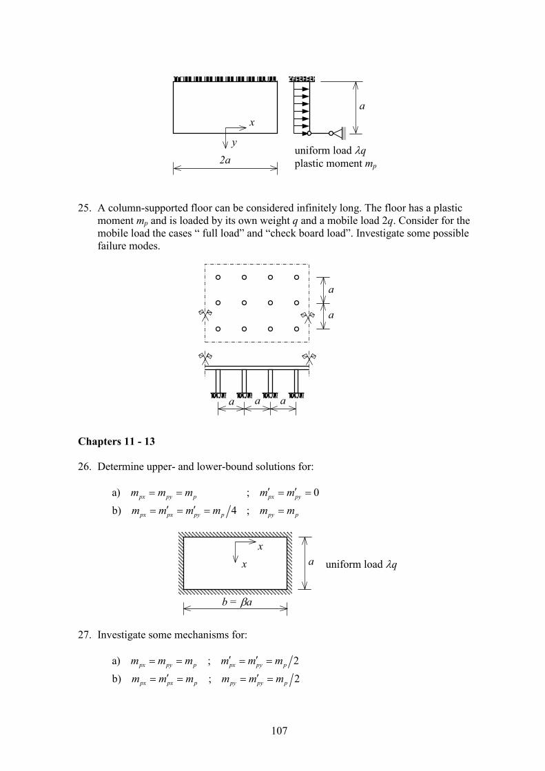
107

25. A column-supported floor can be considered infinitely long. The floor has a plastic

moment mp and is loaded by its own weight q and a mobile load 2q. Consider for the mobile load the cases “ full load” and “check board load”. Investigate some possible failure modes.

Chapters 11 - 13 26. Determine upper- and lower-bound solutions for:

a) ; 0b) 4 ;

px py p px py

px px py p py p

m m m m mm m m m m m

� �� � � �

� �� � � �

27. Investigate some mechanisms for:

a) ; 2b) ; 2

px py p px py p

px px p py py p

m m m m m mm m m m m m

� �� � � �

� �� � � �

a

uniform load �q plastic moment mp 2a

x

y

a a a

a

a

b = �a

a uniform load �q

x x

108

28. Determine upper and lower bounds for the failure load of the drawn plate for the

following cases:

a) All reinforcement moments b) ; 3

p

px p px py py p

mm m m m m m� �� � � �

Hint for the lower-bound calculation: Consider the whole plate as a combination of

two square torsion panels. 29. Given:

A reinforced concrete slab having different reinforcements in the areas I and II . Part I contains at the top and bottom an orthogonal reinforcement mesh according to the xIyI co-ordinate system. The xI-axis makes an angle I with a reference co-ordinate system xy. Similarly part II is reinforced in the xIIyII directions under an angle II. Both plate parts I and II are separated by a straight line. A local co-ordinate system ns is attached to this line. The angle between the n and x-axis is called� . Points with positive n are situated in part I , points with negative n can be found in part II .

b = 2a

a uniform load �q

x

�

s n

IIy

IIx

II�

Iy Ix

I�

sn

x

y

I II

�

a

a

x

y

a

�F

109

Further it is given that a yield line crosses both plate areas (local co-ordinate system ns under angle ). The point S indicates the intersection of the yield line and the separation line. Asked: Show that the yield line does not transmit a distributed transverse load. Prove that the yield line at point S transmits a concentrated transverse force sQ of magnitude: � �� �cot cot withI I II II

s nn ns nn nsQ m m m m� � � � �� � � � � Show that for the special case 0I II

� � �� � � it holds: � �cotI II

s px pxQ m m �� �

30. Determine for the given mechanism the optimal and load factor, both through the work method and the equilibrium method. Do not forget that the yield line besides a concentrated transverse force also transmits torsional moments.

31. In a point of a reinforced concrete slab the following state of moments is present:

10 kN/m30 kN/m

40 kN/m

xx

xy

yy

mmm

�

�

� �

Determine the required upper and lower reinforcement in x- and y-direction if further it

is given that:

s

n

IIy

IIxIy

Ix

I II

sn

x

y

� =

b = 2a

a uniform load �q

12px p

py px py p

m mm m m m

�

� �� � �

x y

a �

110

slab thickness h = 0.20 m concrete quality B 30 reinforcement quality Fe B 220 load factor � = 1.8 32. Again consider question 20. Set q = 4 kN/m2. The load factor � should not be less than

1.8. Starting from the given moment distribution find a suitable reinforcement scheme. Further data: slab thickness h = 0.18 m size a = 4 m concrete quality B 30 steel quality Fe B 400

33. The drawn construction is loaded by its own weight and a useful load of 3 kN/m2. Find

a global dimensioning for the beams and the slab. Choose a transmission system for the load and dimension the main reinforcement accordingly.

load factor � = 1.8 concrete quality B 30 steel quality Fe B 220

34. Give a proper design for the depicted floor for a useful load of 2 kN/m2.

AA

B

B

5 m

3 m

7 m A-A

B-B

7 m 7 m7 m

7 m

7 m

7 m

111

Answers to question 1 – 16

2

2

2

2

2

2

2

2

1. 8

2. 16

3. 2.32

4. 5.55

5. 11.7

6. 59.6

7. 119.2

8. 2

p

p

p

p

p

p

p

p

mqa

mqa

mqamqamqamqa

mqa

mqa

�

�

�

�

�

�

�

�

�

�

�

�

�

�

�

�

2

2

2

2

2 2

2 2

2

2

9. 8

10. 16

11. 2.0

12. _ _

13. 4.0

14. 11.56 26.2

15. 1.77 2

16a. 2

16b. 4

p

p

p

p

p p

p p

p

p

mqa

mqamqa

mqa

m mqa qa

m mqa qa

mqamqa

�

�

�

�

�

�

�

�

�

�

�

�

� �

� �

�

�