Construction of Green's functions for the Boltzmann equations

Shih-Hsien YuDepartment of Mathematics

National University of Singapore

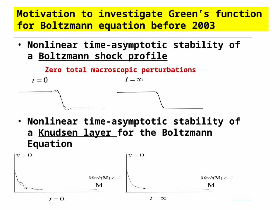
Motivation to investigate Green’s function for Boltzmann equation before 2003

• Nonlinear time-asymptotic stability of a Boltzmann shock profile

Zero total macroscopic perturbations

• Nonlinear time-asymptotic stability of a Knudsen layer for the Boltzmann EquationMach number <-1

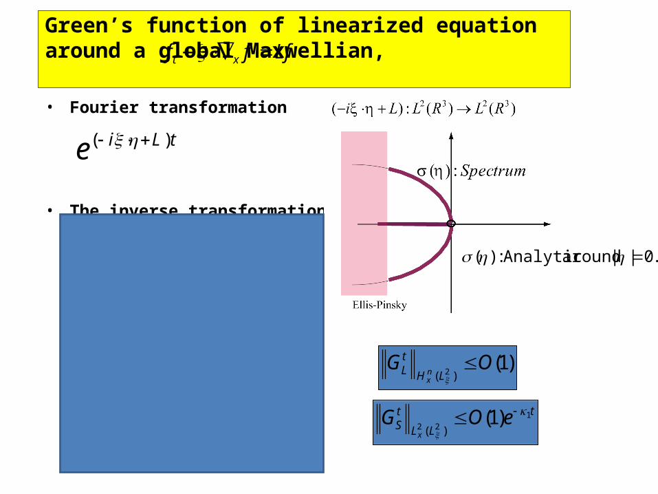
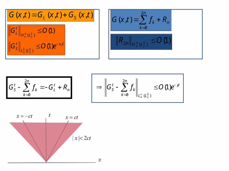
Green’s function of linearized equation around a global Maxwellian,

• Fourier transformation

• The inverse transformation

Lfff xt

tLie )(

.0|| around Analytic :)( detxGR

Litix 3

)(),(

detxG

detxG

txGtxGtxG

LitixS

LitixL

SL

||

)(

||

)(

),(

),(

),(),(),(

t

LL

tS eOG

x

122

)1()(

)1()( 2

OGLH

tL n

x

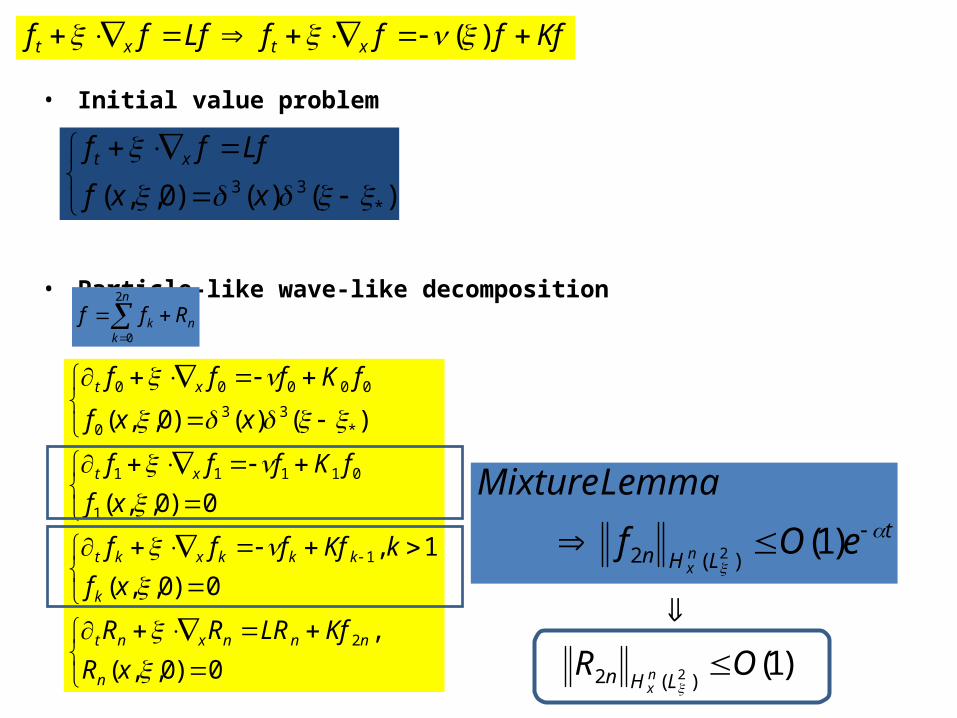
• Initial value problem

• Particle-like wave-like decomposition

KffffLfff xtxt )(

)()()0,,(

*33

xxf

Lfff xt

0)0,,(

,

0)0,,(

1 ,

0)0,,(

)()()0,,(

2

1

1

01111

*33

0

00000

xR

KfLRRR

xf

kKffff

xf

fKfff

xxf

fKfff

n

nnnxnt

k

kkkxkt

xt

xt

n

knk Rff

2

0

t

LHn eOf

LemmaMixture

nx

)1(

)(2 2

)1(

)(2 2 ORLHn n

x

)1( )(2 2 OR

LHn nx

n

knk RftxG

2

0

),(

t

LL

tS

LH

tL

eOG

OG

x

nx

122

2

)1(

)1(

)(

)(

),(),(),( txGtxGtxG SL

ntL

n

kk

tS RGfG

2

0

t

LL

n

kk

tS eOfG

x

)1()(

2

0 2

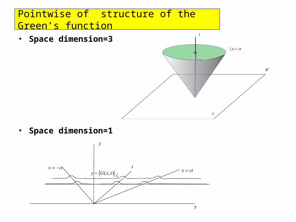
Pointwise of structure of the Green’s function

• Space dimension=3

• Space dimension=1

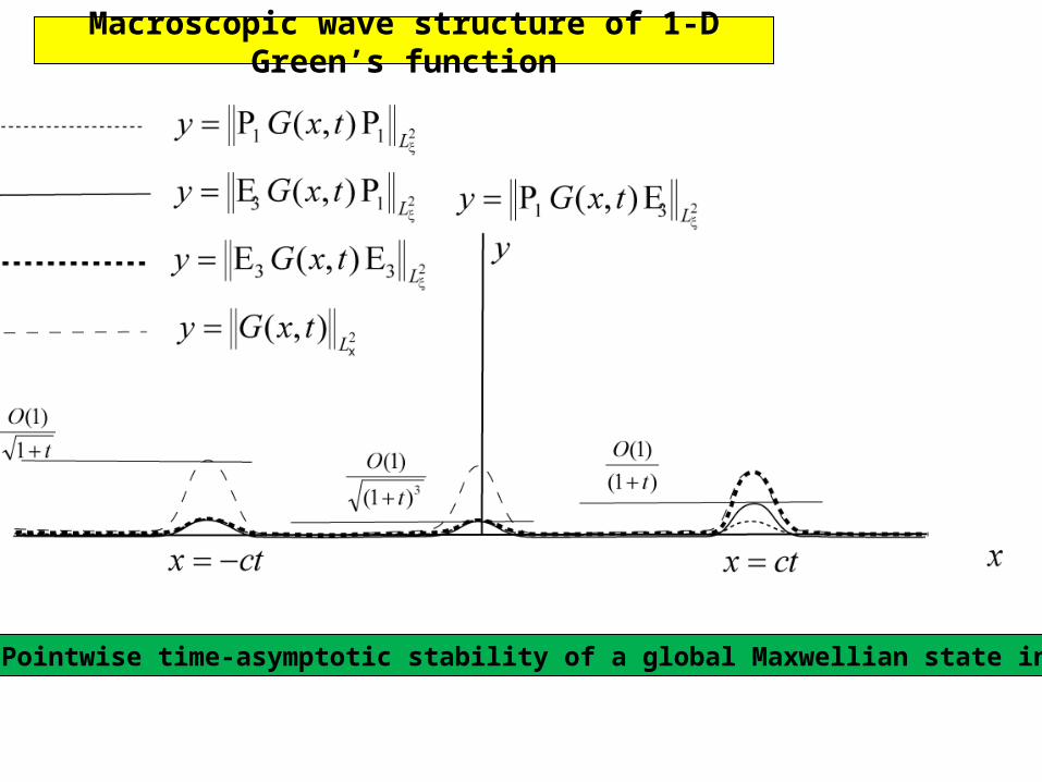
Macroscopic wave structure of 1-D Green’s function

Application: Pointwise time-asymptotic stability of a global Maxwellian state in 1-D.

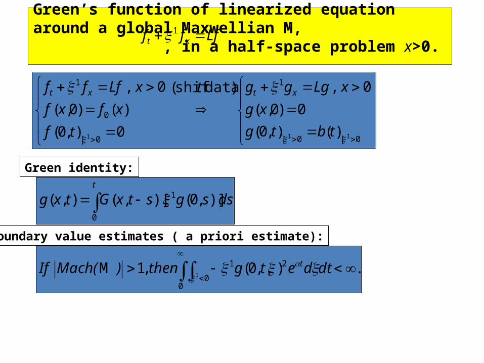
Green’s function of linearized equation around a global Maxwellian M, , in a half-space problem x>0. 1 Lfff xt

0|0|

1

0|

0

1

111 )(),0(

0)0,(

0 ,)data shif(

0),0(

)()0,(

0 ,

tbtg

xg

xLgggt

tf

xfxf

xLfff xtxt

Green identity:

t

dssgstxGtxg0

1 )],0()[,(),(

.),,0( ,1M 2

00

11

dtdetgthen)Mach(If t

Boundary value estimates ( a priori estimate):

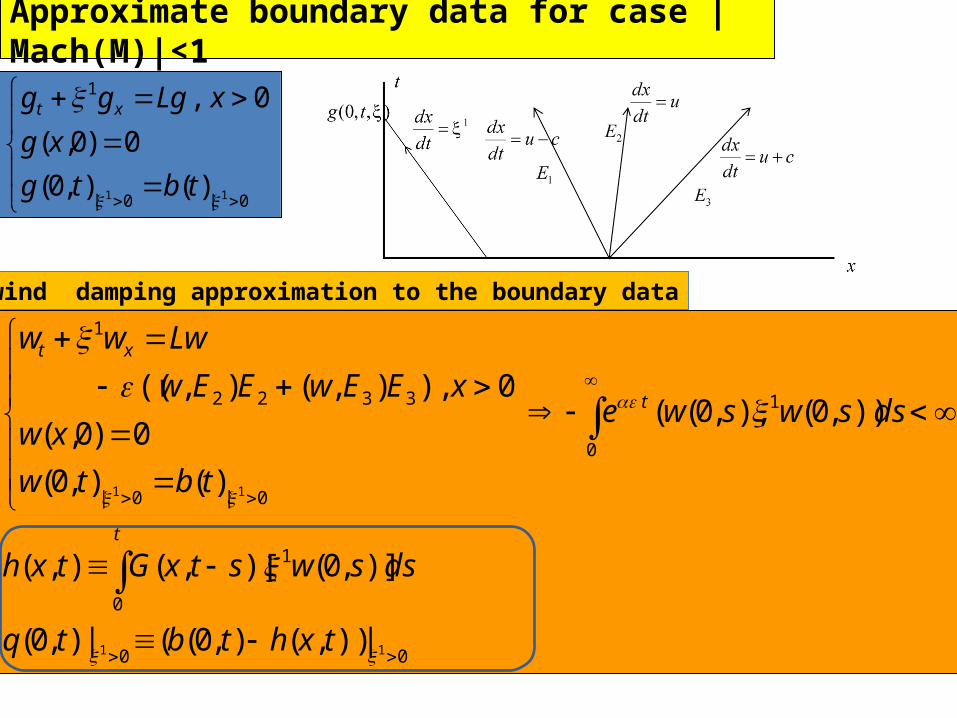
Approximate boundary data for case |Mach(M)|<1

0|0|

1

11 )(),0(

0)0,(

0 ,

tbtg

xg

xLggg xt

Upwind damping approximation to the boundary data

00

0

1

1

0

0|0|

3322

1

11

11

|)),(),0((|),0(

)],0()[,(),(

)),0(),,0((

)(),0(

0)0,(

0 ),),(),((

txhtbtq

dsswstxGtxh

dsswswe

tbtw

xw

xEEwEEw

Lwww

t

t

xt

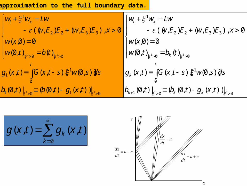
An approximation to the full boundary data.

0101

0

11

0|0|

3322

1

11

11

|)),(),0((|),0(

)],0()[,(),(

)(),0(

0)0,(

0 ),),(),((

txgtbtb

dsswstxGtxg

tbtw

xw

xEEwEEw

Lwww

t

xt

001

0

1

0|0|

3322

1

11

11

|)),(),0((|),0(

)],0()[,(),(

)(),0(

0)0,(

0 ),),(),((

txgtbtb

dsswstxGtxg

tbtw

xw

xEEwEEw

Lwww

kkk

t

k

k

xt

0

),(),(k

k txgtxg

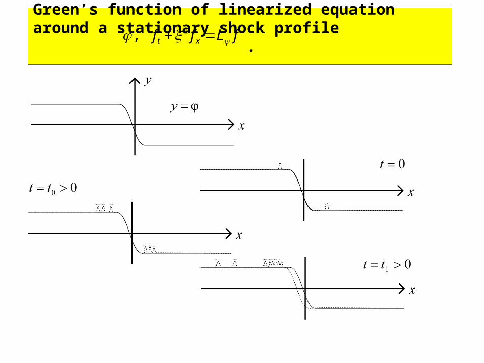
Green’s function of linearized equation around a stationary shock profile . , 1 fLff xt

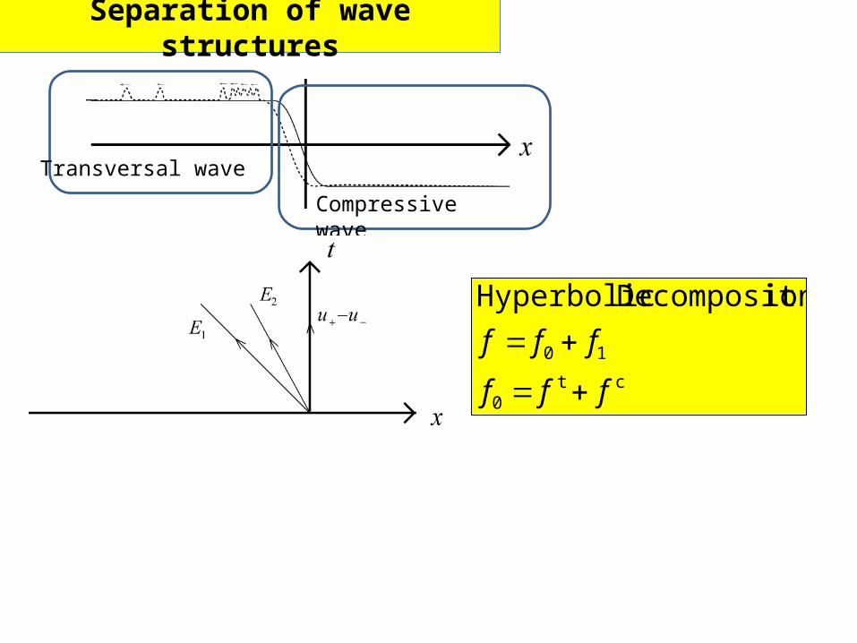
Separation of wave structures

Transversal wave

Compressive wave

ct0

10

ionDecomposit Hyperbolic

fff

fff

1. Shift data

)()0,(

01

xhxf

fLff xt

2)()(

L

xxhy

)]()[(

)]()[(),(

xhGx

xhGxtxgt

t

dyyhtyxGxhG t )(),()]([

gLtx xt )(),( 1

0)0,(

),(),(),(1

xq

qLqq

txgtxftxq

xt

2)(),(

L

xtxgy

2. Hyperbolic Decomposition

ct0

10

ionDecomposit Hyperbolic

fff

fff

0)0,(

1

xq

qLqq xt

Transversal wave

Compressive wave

3. Transverse Operator and Local Wave Front tracing

||

1

t1

)1(

),(][)(

,0),(][)(

:),]([

3,

x

Lxt

xt

eO

txTL

txTL

txT

0

),(])[)((

)(')(),]([

:),]([

10

dxtxDTLP

xtltxD

txD

xt

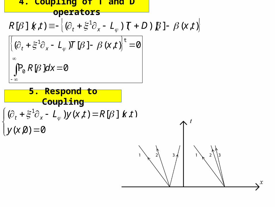
4. Coupling of T and D operators

),(])[)((),]([ 1 txDTLtxR xt

5. Respond to Coupling

0][P

0),(][)(

0

t1

dxR

txTLxt

0)0,(

),]([),()( 1

xy

txRtxyLxt

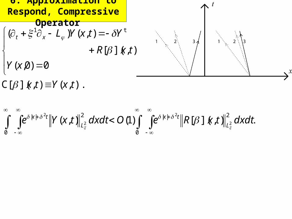
6. Approximation to Respond, Compressive Operator

).,(),](C[

0)0,(

),]([

),()( t1

txYtx

xY

txR

YtxYLxt

.),]([)1(),(2||

0

2||

0

2

2

2

2

dxdttxReOdxdttxYeL

tx

L

tx

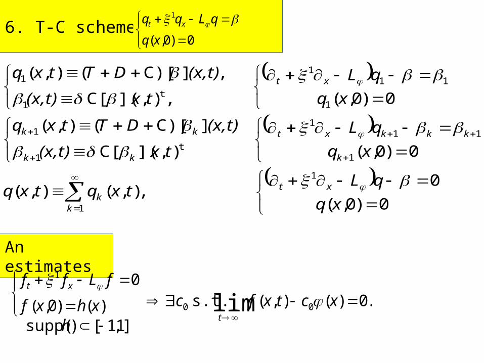
6. T-C scheme for

0)0,(

1

xq

qLqq xt

0)0,(

0 ,),(),(

0)0,(

),](C[

]C)[(),(

0)0,(

,),](C[

, ]C)[(),(

1

1

1

111

t1

1

1

111

t1

1

xq

qLtxqtxq

xq

qL

tx(x,t)

(x,t)DTtxq

xq

qL

tx(x,t)

(x,t)DTtxq

xt

kk

k

kkkxt

kk

kk

xt

An estimates

.0)(),( s.t.

]1,1[)supp()()0,(

0

00

1

lim

xctxfc

hxhxf

fLff

t

xt

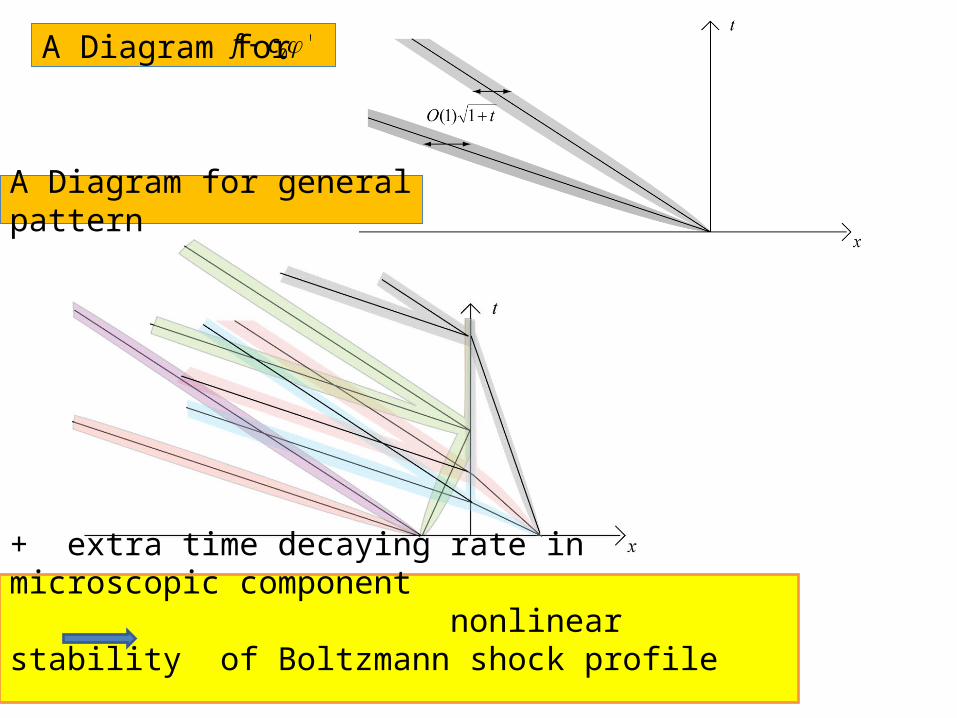
A Diagram for '0cf

A Diagram for general pattern

+ extra time decaying rate in microscopic component nonlinear stability of Boltzmann shock profile

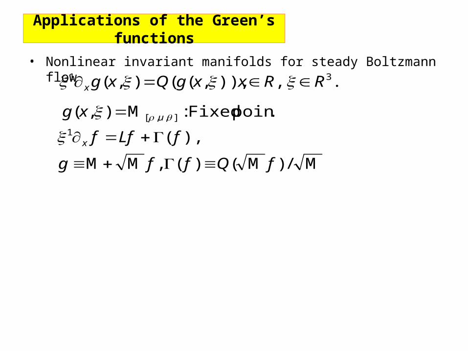
Applications of the Green’s functions

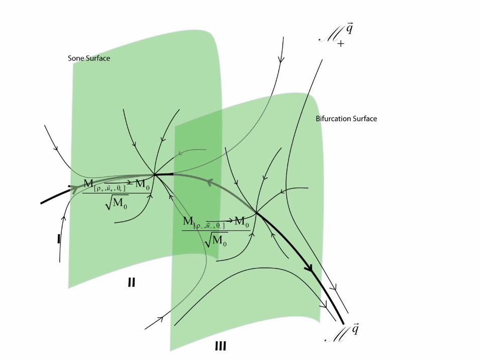
• Nonlinear invariant manifolds for steady Boltzmann flow

. , )),,((),( 31 RRxxgQxgx

.point Fixed :M),( ],,[ uxg

M/)M()( ,MM

),(1

fQffg

fLffx

Applications of the Green’s functions

• Milne’s problme

],,[

0|0|

31

M),(lim

given :)(),0(

,0 )),,((),(

11

ux

x

xg

bg

RxxgQxg

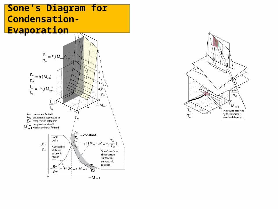
Sone’s Diagram for Condensation-Evaporation