PSYCHOMETRIKA2013DOI: 10.1007/S11336-013-9385-6

CONSTRAINED STOCHASTIC EXTENDED REDUNDANCY ANALYSIS

WAYNE S. DESARBO

PENNSYLVANIA STATE UNIVERSITY

HEUNGSUN HWANG

MCGILL UNIVERSITY

ASHLEY STADLER BLANK AND EELCO KAPPE

PENNSYLVANIA STATE UNIVERSITY

We devise a new statistical methodology called constrained stochastic extended redundancy anal-ysis (CSERA) to examine the comparative impact of various conceptual factors, or drivers, as well asthe specific predictor variables that contribute to each driver on designated dependent variable(s). Thetechnical details of the proposed methodology, the maximum likelihood estimation algorithm, and modelselection heuristics are discussed. A sports marketing consumer psychology application is provided in aMajor League Baseball (MLB) context where the effects of six conceptual drivers of game attendanceand their defining predictor variables are estimated. Results compare favorably to those obtained usingtraditional extended redundancy analysis (ERA).

Key words: redundancy analysis, maximum likelihood estimation, sports marketing, Major League Base-ball, consumer psychology.

1. Introduction

The sports industry is one of the top 10 business sectors in the US in terms of both size andgrowth (DeSarbo, 2009) and is valued at $470 billion (Plunkett Research, 2013). The applicationin this paper deals specifically with Major League Baseball (MLB) whose 30 teams generatedan estimated $6.8 billion in revenue in 2012 alone (Badenhausen, Ozanian, & Settimi, 2013).However, league wide attendance is down almost 3 % a quarter of the way into the 2013 seasonwith over half of the league’s teams reporting losses (Sports Business Journal, 2013). As almostone-third of MLB teams’ total gross revenues come from gate receipt, attendance has the poten-tial to either make or break many MLB teams financially. Thus, determining the factors that driveattendance is of great importance to MLB and its teams.

The current research seeks to develop a number of conceptual factors or drivers that influ-ence consumer behavior to attend MLB games based on past sports marketing and consumerpsychology research. We utilize various predictor variables to define each of these drivers. Wethen devise a new multivariate statistical procedure we call constrained stochastic extended re-dundancy analysis (CSERA), which is designed to quantify the impact of these various drivers aswell as their component predictor variables, in an effort to obtain greater insight into the impacton consumers’ MLB attendance.

CSERA has several strengths and advantages over competing methods. First, it incorporatesformative relationships between the explanatory variables and conceptual drivers, as well as re-flective relationships between the conceptual drivers and the dependent variable(s). Second, it

Requests for reprints should be sent to Wayne S. DeSarbo, Marketing Department, Smeal College of Business,Pennsylvania State University, University Park, PA 16802, USA. E-mail: wsd6@psu.edu

© 2013 The Psychometric Society

PSYCHOMETRIKA

can handle a very large number of explanatory variables even when there are a small number ofobservations (as is the case with most professional sports seasons). Third, it handles collinearityby reducing the rank of the regression as it forms a limited number of components from eachset of variables. Moreover, these different components are constrained to be orthogonal to eachother. Fourth, it is able to accommodate various linear parameter restrictions regarding the impactof the various drivers and/or their composite variables. These qualities are particularly relevantfor the MLB application we present. We devise a penalized maximum likelihood estimation pro-cedure that provides asymptotic standard errors directly without requiring a resampling methodand integrates regularization to address potential collinearity in each set of explanatory variables.

The remainder of the paper is organized as follows. In Section 2, we briefly review the litera-ture related to the various drivers of MLB attendance and devise an overall conceptual frameworkfor general application. In Section 3, we describe the Pittsburgh Pirates MLB team as well as thespecific data (predictor variables for each of the major drivers) collected and included in the anal-ysis. In Section 4, we present the technical details of our new CSERA modeling framework andconceptually compare it to related methodology in the statistical and psychometric literatures.We describe the maximum likelihood estimation framework, the various constraints allowed toimprove the interpretability of the solution, and the associated model selection heuristics. In Sec-tion 5, we apply our CSERA methodology to the Pittsburgh Pirates data for the 2010, 2011,and 2012 seasons, and present the most parsimonious solution obtained. The detailed results andrespective managerial insights are discussed. In Section 6, we present a comparison of results ob-tained from Takane and Hwang’s (2005) deterministic extended redundancy analysis (ERA) andhighlight several key differences in the insights provided by each method. Finally, in Section 7,we present an overall summary and suggest a number of directions for future research.

2. MLB Attendance Drivers

Several recent research papers have examined a variety of MLB attendance drivers relatedto consumers’ decisions to attend MLB games (see Beckman, Cai, Esrock, & Lemke, 2012;DeSarbo, Stadler Blank, & McKeon, 2012; Lemke, Leonard, & Tlhokwane, 2010), including theimpact that team performance, the opponent, in-game promotions, venue, weather, and mediaalternatives have on MLB attendance. We briefly discuss each of these six major conceptualfactors affecting MLB attendance below.

Overall, the most studied attendance driver is that of team performance in which a positiverelationship between performance and attendance has been well established (Baade & Tiehen,1990; Becker & Suls, 1983; Beckman et al., 2012; Greenstein & Marcum, 1981; Hansen & Gau-thier, 1989; Hill, Madura, & Zuber, 1982; Lemke et al., 2010). In fact, Greenstein and Marcum(1981) found that team performance variables accounted for 25 % of the variation in season-longMLB National League attendance. Furthermore, both objective and relative performance metricshave been found to positively influence attendance (Becker & Suls, 1983; Hansen & Gauthier,1989).

Prior research has also demonstrated a uniformly positive relationship between the attrac-tiveness and/or quality of the opposing team (as well as its players) and attendance (Baade &Tiehen, 1990; Beckman et al., 2012; Hill et al., 1982; Lemke et al., 2010; Marcum & Greenstein,1985). Interleague play has also been associated with increases in attendance (Beckman et al.,2012; Lemke et al., 2010).

A number of studies have also addressed the positive relationship between in-game pro-motions and attendance (Baade & Tiehen, 1990; Barilla, Gruben, & Levernier, 2008; Boyd &Krehbiel, 2003; Hill et al., 1982; Lemke et al., 2010; Marcum & Greenstein, 1985; McDon-ald & Rascher, 2000). Several studies have uncovered average increases in attendance of up to

WAYNE S. DESARBO ET AL.

20 % at MLB games when a promotion is employed (Boyd & Krehbiel, 2003). Prior work hasalso suggested that promotions provide additional value for games that experience low demand(e.g., day/weekday games or games against unattractive opponents) (Boyd & Krehbiel, 2003), forpoorer performing teams (Marcum & Greenstein, 1985), and for teams in small markets (Lemkeet al., 2010). As promotional activities are one of the only attendance drivers that teams can di-rectly control, a number of recent studies have focused on optimizing MLB teams’ promotionalschedules (e.g., DeSarbo et al., 2012; Kappe, Stadler Blank, & DeSarbo, 2014). The importanceof this work can be inferred by the widespread use of promotions in MLB. In 2012, the 30 MLBteams implemented more than 2,250 promotions, such as bobbleheads, caps, t-shirts, concerts,fireworks, price discounts, etc. (Broughton, 2012).

Venue and weather essentially represent comfort and convenience factors. Generally speak-ing, these factors are positively associated with increases in attendance. As defined in the currentstudy, venue includes game schedule characteristics such as game time, day of the week, month,year, and holidays. Past research has established a positive relationship between attendance andevening games, weekend games, games played in the summer or on national holidays, and gamesplayed in the latter part of the season for teams with a solid chance of playoff contention (Barillaet al., 2008; Boyd & Krehbiel, 2003; Hansen & Gauthier, 1989; Hill et al., 1982; Lemke et al.,2010; Marcum & Greenstein, 1985).

Concerning weather, some prior work has recognized the negative impact of inclementweather on sports attendance, especially as it relates to women’s attendance (Siegfried & Hin-shaw, 1977; Trail, Robinson, & Kim, 2008). This effect holds for both low temperatures andthe presence of precipitation. Other studies, however, have failed to establish a significant rela-tionship between weather and professional sports attendance (Baimbridge, Cameron, & Dawson,1996; Bird, 1982). It is conceivable that small amounts of pregame precipitation during the hotsummer months may have a beneficial effect on attendance in terms of its cooling effects (e.g.,Welki and Zlatoper (1999) found that increased temperatures decreased the negative impact ofrain on attendance).

Several studies have also examined the availability of games on television and substituteforms of entertainment. Evidence regarding the effect of televised games on attendance is mixed,as some studies failed to establish that any relationship exists (Hill et al., 1982; Siegfried &Hinshaw, 1977, 1979); whereas others found a negative relationship between the availability ofgames on television and attendance (Allan, 2004; Baimbridge et al., 1996; Fizel & Bennett, 1989;Zhang & Smith, 1997). However, none of these studies quantitatively differentiated the effectsof games that are nationally versus locally televised. Nationally televised games are typicallyreserved for highly competitive games between teams in contention in the standings (at the timeof broadcast), which may be associated with higher attendance due to the attractiveness of thegames. Substitute forms of entertainment (including other professional sports teams and events)have been uniformly associated with lower levels of attendance (Baade & Tiehen, 1990; Gitter& Rhoads, 2010; Hansen & Gauthier, 1989; Hill et al., 1982; Trail et al., 2008).

Although there are other attendance drivers related to demographic and socioeconomic fac-tors, we do not include these variables in our model since this case study is restricted to one teamand all observations represent home games played in Pittsburgh. Thus, there is no significantvariation present in our data. In addition, we do not include pricing in our modeling effort for thesame reason, as the Pittsburgh Pirates did not fully implement dynamic pricing until 2013 (i.e.,game pricing was relatively static within each season).

Keeping these six conceptual MLB attendance drivers in mind (performance, opponent, pro-motion, venue, weather, and media), the next section will briefly describe the Pittsburgh Piratesand the team-specific data that were collected to measure the various aspects of the six attendancedrivers.

PSYCHOMETRIKA

TABLE 1.Promotions employed by the Pittsburgh Pirates.

Promotion 2010 2011 2012

Bobblehead 1 1 1Bottle 1Bowl 1Canvas wrap/print 3 1Cap 5 2 2Coffee clutch 1Concert 5 4 4Cooler 1Figurine/bust 2 1Fireworks 8 9 8Fleece blanket 1 1Gloves/scarf set 1Kids 12 13 13Magnetic schedule 4 2 2Mom 1 1 1Poster/wall calendar 1 2Price package (i.e., Buc Night) 1 1 1Stein 1 1Theme day 3Tote bag 1Towel 1T-shirt 10 13 12Umbrella 1Total: 63 52 47

Note: Fifty-two of 81 home games in 2010, 42 of 80 home games in 2011, and 39 of 80 home games in 2012employed at least one promotion. We only have data on 80 games (as opposed to 81) for 2011 and 2012since games 126 and 17, respectively, were rescheduled as double headers in which separate attendancefigures were not reported. Neither game included a promotion.

3. The Pittsburgh Pirates 2010–2012 Data

The data collected for this study include a number of variables related to the Pittsburgh Pi-rates’ 2010, 2011, and 2012 seasons. The Pittsburgh Pirates is one of 30 professional MLB teamsand plays in the Central Division of the National League. The team enjoyed some past success,reflected by 14 past playoff appearances, nine pennants, and five World Series championships(Baseball-Reference.com, 2013). However, more recent performance has deteriorated, resultingin the accumulation of 20 consecutive losing seasons—a record in North American professionalsports for the most consecutive losing seasons (Dvorchak, 2008).

Based on the six major drivers of MLB attendance discussed previously, specific measure-ment items/predictor variables were organized into one of the six attendance drivers: perfor-mance, opponent, promotion (see Table 1 for specific promotions employed), venue, weather,and media (see Table 2 for specific items examined in the initial analysis). Note, for the Pitts-burgh Pirates and the vast majority of teams in MLB, promotions are set well in advance of thebeginning of the season each year to promote advance ticket sales and are rarely altered duringthe course of the season. This limits concerns for potential endogeneity.

In the current work, we have specific interest in examining the impact that each predic-tor variable has on its respective driver, as well as the impact that each driver has on overallattendance. Ultimately, we are interested in the effects of our predictor variables and drivers

WAYNE S. DESARBO ET AL.

TABLE 2.Initial predictor variables included in the six attendance drivers.

AttendanceDriver

Variable

Performance Pirates winning percentagePirates 10-game winning percentagePirates season-long winning percentage vs. opponentPirates streak (consecutive wins vs. losses)Pirates games back (vs. division leader)

Opponent 22 Opponents played by the PiratesPromotion 23 Promotions employed by the PiratesVenue Time of day

Day of the weekMonthSeasonHoliday

Weather Mean temperatureTotal precipitationPresence of precipitationComfort index (interaction of temperature and precipitation)

Media Game broadcast on local TV (regional sports network restricted to the local market)Game broadcast on national TV (national network/cable channel available in all markets)Presence of other “Big 4” professional sporting events in Pittsburgh (here, NFL and NHL)

on game attendance—which is defined by MLB as the number of tickets sold for each game(including tickets purchased by season and single-game ticket holders). Data for the three Pitts-burgh Pirates seasons under investigation were collected from the following archival sources:http://pittsburgh.pirates.mlb.com/index.jsp?c_id=pit, www.baseball-reference.com/teams/PIT/,www.farmersalmanac.com/weather-history/, http://www.pro-football-reference.com/teams/pit/,and http://www.hockey-reference.com/teams/PIT/.

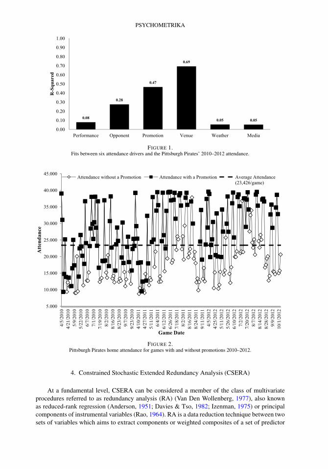
Before applying our newly proposed methodology, we conducted a preliminary analysis ofthe six attendance drivers across all three seasons (2010, 2011, and 2012) by separately regressingattendance on each set of predictor variables from each of the six attendance drivers. Figure 1displays the fits from each of the six regressions. Venue had the greatest impact on game at-tendance, followed by promotions, opponent, performance, weather, and media. All attendancedrivers are significant at p < 0.01. The results also indicate that the attendance drivers are inter-correlated since the sum of the R-squares exceeds one. An aggregate regression analysis obtainedby regressing attendance on all the predictor variables from the six different drivers produced amaximum condition index of 115.22 indicating severe collinearity. Thus, in order to estimate thedifferential impact of each driver set and their respective predictor variables, a method that canaccommodate collinear predictor variables and still preserve the six driver theoretical structure isrequired.

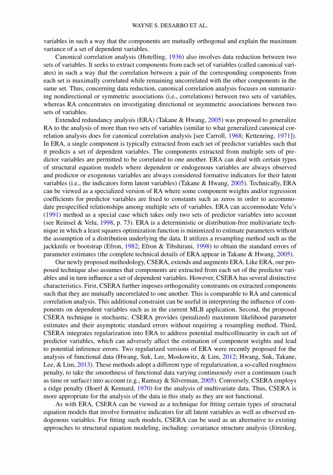
It is worth noting that promotions had the second highest impact on game attendance forthe Pirates. This is good news for team management, considering it is the only attendance driverMLB teams have absolute control over. The influence promotions have on season-long atten-dance can also be observed in Figure 2. In order for the Pirates to go above the average atten-dance (i.e., attendance above the horizontal dashed line), a promotion is almost always present.However, it appears that a promotion alone is not indicative of attendance above the average, asa number of games with promotions fell below the horizontal line. Thus, it remains imperative toexamine all six attendance drivers, in addition to the predictor variables that define them, in aneffort to enhance overall MLB team attendance.

PSYCHOMETRIKA

FIGURE 1.Fits between six attendance drivers and the Pittsburgh Pirates’ 2010–2012 attendance.

FIGURE 2.Pittsburgh Pirates home attendance for games with and without promotions 2010–2012.

4. Constrained Stochastic Extended Redundancy Analysis (CSERA)

At a fundamental level, CSERA can be considered a member of the class of multivariateprocedures referred to as redundancy analysis (RA) (Van Den Wollenberg, 1977), also knownas reduced-rank regression (Anderson, 1951; Davies & Tso, 1982; Izenman, 1975) or principalcomponents of instrumental variables (Rao, 1964). RA is a data reduction technique between twosets of variables which aims to extract components or weighted composites of a set of predictor

WAYNE S. DESARBO ET AL.

variables in such a way that the components are mutually orthogonal and explain the maximumvariance of a set of dependent variables.

Canonical correlation analysis (Hotelling, 1936) also involves data reduction between twosets of variables. It seeks to extract components from each set of variables (called canonical vari-ates) in such a way that the correlation between a pair of the corresponding components fromeach set is maximally correlated while remaining uncorrelated with the other components in thesame set. Thus, concerning data reduction, canonical correlation analysis focuses on summariz-ing nondirectional or symmetric associations (i.e., correlations) between two sets of variables,whereas RA concentrates on investigating directional or asymmetric associations between twosets of variables.

Extended redundancy analysis (ERA) (Takane & Hwang, 2005) was proposed to generalizeRA to the analysis of more than two sets of variables (similar to what generalized canonical cor-relation analysis does for canonical correlation analysis [see Carroll, 1968; Kettenring, 1971]).In ERA, a single component is typically extracted from each set of predictor variables such thatit predicts a set of dependent variables. The components extracted from multiple sets of pre-dictor variables are permitted to be correlated to one another. ERA can deal with certain typesof structural equation models where dependent or endogenous variables are always observedand predictor or exogenous variables are always considered formative indicators for their latentvariables (i.e., the indicators form latent variables) (Takane & Hwang, 2005). Technically, ERAcan be viewed as a specialized version of RA where some component weights and/or regressioncoefficients for predictor variables are fixed to constants such as zeros in order to accommo-date prespecified relationships among multiple sets of variables. ERA can accommodate Velu’s(1991) method as a special case which takes only two sets of predictor variables into account(see Reinsel & Velu, 1998, p. 73). ERA is a deterministic or distribution-free multivariate tech-nique in which a least squares optimization function is minimized to estimate parameters withoutthe assumption of a distribution underlying the data. It utilizes a resampling method such as thejackknife or bootstrap (Efron, 1982; Efron & Tibshirani, 1998) to obtain the standard errors ofparameter estimates (the complete technical details of ERA appear in Takane & Hwang, 2005).

Our newly proposed methodology, CSERA, extends and augments ERA. Like ERA, our pro-posed technique also assumes that components are extracted from each set of the predictor vari-ables and in turn influence a set of dependent variables. However, CSERA has several distinctivecharacteristics. First, CSERA further imposes orthogonality constraints on extracted componentssuch that they are mutually uncorrelated to one another. This is comparable to RA and canonicalcorrelation analysis. This additional constraint can be useful in interpreting the influence of com-ponents on dependent variables such as in the current MLB application. Second, the proposedCSERA technique is stochastic. CSERA provides (penalized) maximum likelihood parameterestimates and their asymptotic standard errors without requiring a resampling method. Third,CSERA integrates regularization into ERA to address potential multicollinearity in each set ofpredictor variables, which can adversely affect the estimation of component weights and leadto potential inference errors. Two regularized versions of ERA were recently proposed for theanalysis of functional data (Hwang, Suk, Lee, Moskowitz, & Lim, 2012; Hwang, Suk, Takane,Lee, & Lim, 2013). These methods adopt a different type of regularization, a so-called roughnesspenalty, to take the smoothness of functional data varying continuously over a continuum (suchas time or surface) into account (e.g., Ramsay & Silverman, 2005). Conversely, CSERA employsa ridge penalty (Hoerl & Kennard, 1970) for the analysis of multivariate data. Thus, CSERA ismore appropriate for the analysis of the data in this study as they are not functional.

As with ERA, CSERA can be viewed as a technique for fitting certain types of structuralequation models that involve formative indicators for all latent variables as well as observed en-dogenous variables. For fitting such models, CSERA can be used as an alternative to existingapproaches to structural equation modeling, including: covariance structure analysis (Jöreskog,

PSYCHOMETRIKA

1973), partial least squares path modeling (Lohmöller, 1989; Wold, 1975, 1982), and general-ized structured component analysis (Hwang & Takane, 2004). In general, covariance structureanalysis is not well-suited for formative indicators because it builds on a factor analysis whereindicators are reflective (i.e., latent variables underlie indicators). Partial least squares path mod-eling and generalized structured component analysis have no difficulty in dealing with formativeindicators. However, both approaches are different from CSERA in that they are deterministic ordistribution-free, whereas CSERA is stochastic or parametric. This parametric feature of CSERAcan help estimate asymptotic standard errors without using a resampling method. In addition, thisparametric feature permits the use of various popular information heuristics for model selection.

We begin by describing the CSERA model for our data. For now, assume that a single com-ponent is specified for each driver set, which has an impact on a single dependent variable (Pirateshome game attendance). We also require that all six drivers are mutually orthogonal to one an-other, a restriction that is needed given the collinearity between many of the items within thedifferent sets of predictor variables (for example, some promotions were only given on certaindays of the week [e.g., kids promotions on Sundays]). Let yi denote the dependent variable value(attendance) measured on the ith home game (i = 1, . . . ,N ). Let xik = [xik1, . . . , xikPk

] denotea Pk by 1 vector of the kth set of predictor variables on the ith home game (k = 1, . . . ,K). Forour data, there are six sets of predictor variables, i.e., K = 6. Let wk = [wki, . . . ,wkPk

]′ denotea Pk by 1 vector of component weights assigned to the kth set of predictor variables. Let bk

denote a regression coefficient value relating a component of the kth set of predictor variables tothe dependent variable. Let ei denote an error for yi . We assume that ei ∼ N(0, σ 2) and that thedependent variable and all predictor variables are normalized with their lengths being unity.

The CSERA model is then given as:

yi =K∑

k=1

[Pk∑

p=1

xikpwkp

]bk + ei

=K∑

k=1

w′kxikbk + ei

=K∑

k=1

fikbk + ei, (1)

subject to the orthogonality constraint on components,∑N

i=1 f 2ik = 1, and

∑Ni=1 fikfih = 0

(k �= h), where fik = [∑Pk

p=1 xikpwkp] = w′kxik indicates the ith component score of the kth

set of predictor variables.To estimate the parameters in CSERA, we seek to maximize a penalized log-likelihood

criterion:

φ =N∑

i=1

logg(yi) − 1

2λ

K∑

k=1

(w′

kwk

), (2)

where g(yi) denotes the density function for yi drawn from a univariate normal distribution,and λ is a determined ridge parameter. This criterion can be considered the L2-norm penalizedlog-likelihood (e.g., Cessie & Houwelingen, 1992; Lee & Silvapulle, 1988).

WAYNE S. DESARBO ET AL.

Maximizing (2) via iteratively reweighted least squares (IRLS) (see Green, 1984) is equiva-lent to minimizing the following penalized least squares criterion:

φ1 =N∑

i=1

(yi −

K∑

k=1

w′kxkbk

)2

+ λ

K∑

k=1

(w′

kwk

)

= (y − Fb)′(y − Fb) + λ

K∑

k=1

(w′

kwk

), (3)

with respect to wk and bk , subject to∑N

i=1 f 2ik = 1 and

∑Ni=1 fikfih = 0, or equivalently F′F = I,

where y = [y1, . . . , yN ]′, b = [b1, . . . , bK ]′, and F = [f1, . . . , fN ]′. The penalty term in (3), of-ten called the ridge penalty (e.g., Hoerl & Kennard, 1970), is added to address potential mul-ticollinearity in each set of predictor variables, which can adversely affect the estimation ofcomponent weights. The ridge penalty takes the magnitudes of the component weights into ac-count. When two predictor variables are highly correlated, a very large positive weight estimatefor one predictor variable can be negated by a very large negative weight estimate for the otherpredictor variable. When the absolute values of the weight estimates are large, the penalty termbecomes large. The ridge parameter (λ) plays a role in balancing out the relative importance ofthe penalty term in the estimation of the weights. If the ridge parameter value becomes large, agreater penalty is imposed on the sizes of the weight estimates, reducing them toward zero. Thus,adding the ridge penalty keeps the magnitudes of the component weights within a certain rangeand addresses the adverse consequences of multicollinearity.

To minimize (3), we use an iterative algorithm similar to the alternating regularized leastsquares algorithm (e.g., Hwang, 2009). This algorithm alternates between the following two stepsuntil there are no substantial changes in parameter estimates between the previous and currentiterations:

Step 1: We update b for fixed wk . This is equivalent to minimizing:

φ2 = (y − Fb)′(y − Fb), (4)

with respect to b, subject to F′F = I. Hence, the estimates of b are obtained by:

b = F′y. (5)

Step 2: We update wk for fixed b. The criterion in (3) can be written as:

φ1 = (y − Fb)′(y − Fb) + λ

K∑

k=1

w′kwk

=⎛

⎜⎝y − [X1, . . . ,XK ]⎡

⎢⎣w1

. . .

wK

⎤

⎥⎦b

⎞

⎟⎠

′ ⎛⎜⎝y − [X1, . . . ,XK ]

⎡

⎢⎣w1

. . .

wK

⎤

⎥⎦b

⎞

⎟⎠

+ λw′w= (y − XWb)′(y − XWb) + λw′w= (

y − (b′ ⊗ X

)vec(W)

)′(y − (b′ ⊗ X

)vec(W)

) + λw′w= (y − Mw)′(y − Mw) + λw′w, (6)

where

X = [X1, . . . ,XK ], W =⎡

⎢⎣w1

. . .

wK

⎤

⎥⎦ ,

PSYCHOMETRIKA

⊗ indicates the Kronecker product, w is the vector formed by eliminating any fixed elementssuch as zeros from vec(W), and M is the matrix formed by eliminating the columns of b′ ⊗ Xcorresponding to the fixed elements in vec(W). Note, Xk is not required to be of full rank.

Then, the estimates of w are obtained by:

w = (M′M + λI

)−1M′y. (7)

Subsequently, we obtain F by fk = Xkwk and orthonormalize F by the Gram–Schmidt orthonor-malization method: Let F∗ denote the orthonormalized F. Then, F∗ = FR−1, where R is ob-tained from the Cholesky factorization of F′F = RR′. Thus, the proposed algorithm is iterative,in which two steps are carried out in each major iteration. The second step is used for updatingthe component weights. Once the weights are updated, the component scores are obtained andorthonormalized. In the next iteration, the weights are again updated, taking into account theorthonormalized components. The asymptotic covariance matrix of the maximum likelihood pa-rameter estimates are obtained at convergence by inverting the negative Hessian matrix computedby using the profile likelihoods (Richards, 1961; also see Yee & Hastie, 2003).

Before applying the iterative algorithm, we need to determine the value of the ridge pa-rameter (λ). We use J -fold cross validation (Hastie, Tibshirani, & Friedman, 2009, p. 214) tochoose the value of λ. In J -fold cross validation, we split the entire set of data into J subsets.We allocate the j th set to the validation set (j = 1, . . . , J ) and use the remaining J − 1 subsetsas a calibration set to estimate parameters under a given value of λ. We apply the parameterestimates to the j th validation set and calculate the (minus) log-likelihood value. We repeat thisprocedure for J validation sets and compute the average of the J (minus) log-likelihood valuesas the cross-validation score for the given value of λ. The value of λ associated with the smallestcross-validation score is selected.

Finally, we utilize various information heuristics such as the AIC, BIC, and CAIC for modelselection to identify the most parsimonious number of components per driver set (Wedel & De-Sarbo, 1995).

5. Analysis of the Pittsburgh Pirates 2010–2012 Data

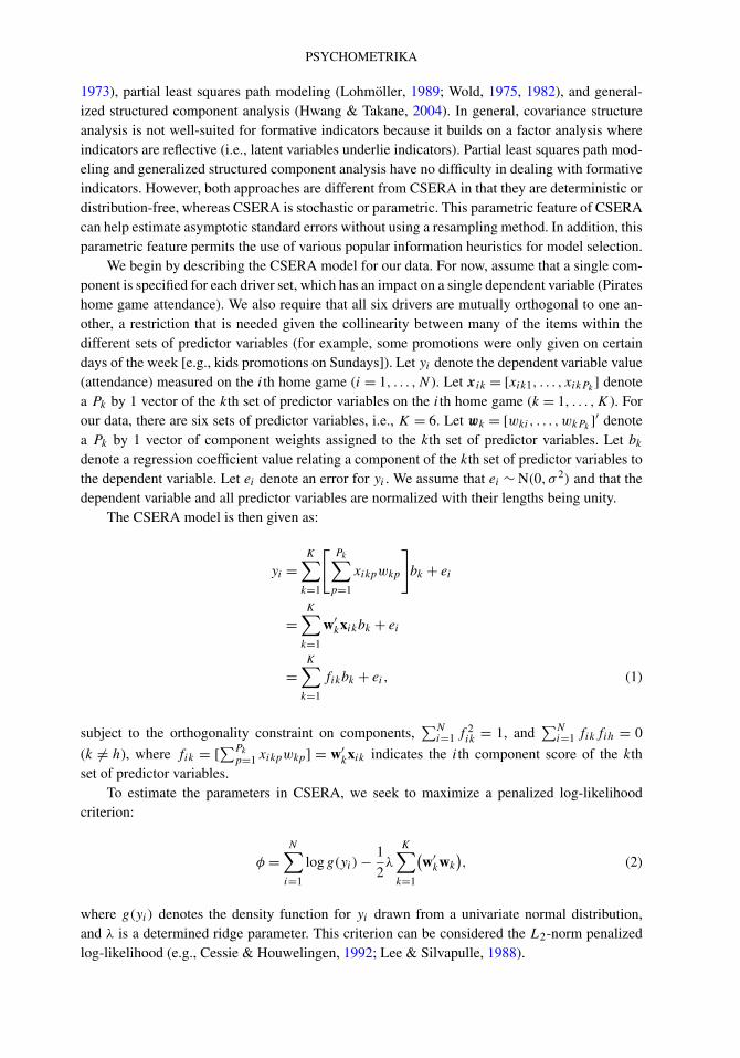
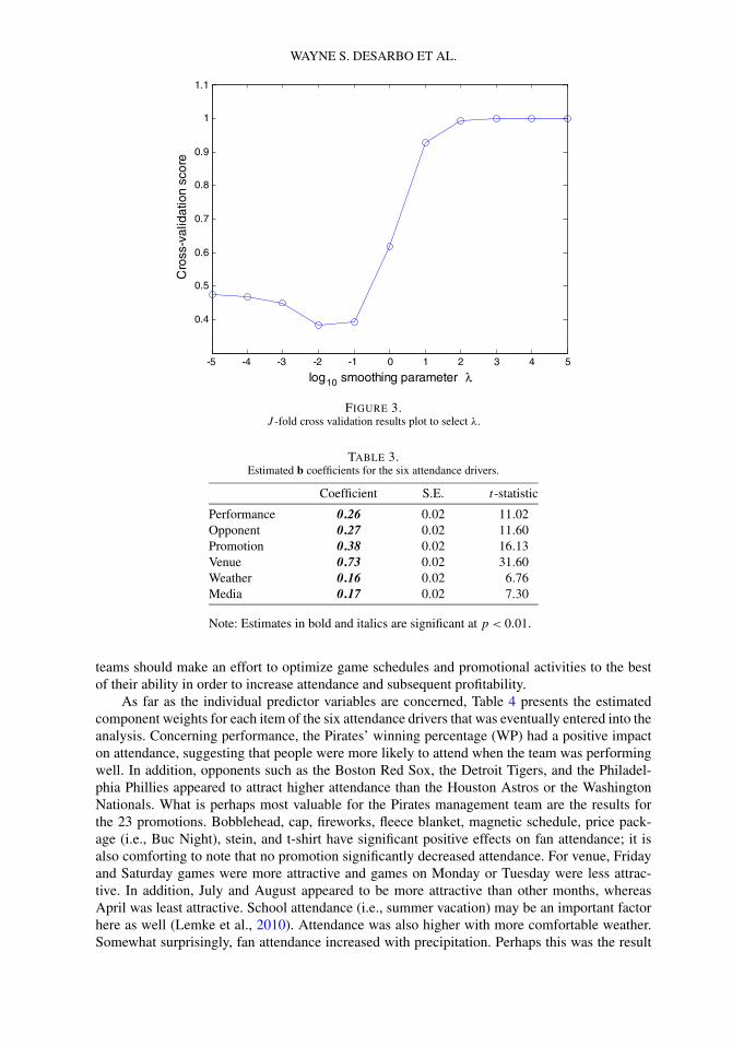
We apply the CSERA methodology described above to the six conceptual drivers of atten-dance, as measured by the many predictor variables discussed, using attendance as the depen-dent variable. We estimate the CSERA model jointly on the 2010, 2011, and 2012 seasons for thePittsburgh Pirates which includes 241 home games and a total of 74 predictor variables across thesix drivers. In applying the J -fold cross validation procedure to select the ridge parameter (λ),we obtained the plot shown in Figure 3. This figure displays the cross validation scores againstthe common logarithms of different values of λ. As shown in this figure, the minimum value wasachieved at λ = 0.01 (log10(−2) = 0.01). Thus, we used λ = 0.01 for the analysis of the data.

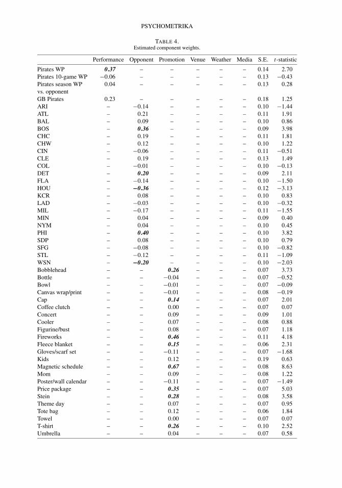
In testing the optimal number of components for each driver set, the one component solu-tion for each driver set was the most parsimonious solution obtained in the analysis. The solutionrendered the following: AIC = 160.12, BIC = 438.91, CAIC = 439.24. Table 3 presents the esti-mated regression coefficients for each of the six conceptual drivers of attendance. All six drivershave a positive and significant effect on attendance. Venue appears to be the most importantdriver of the Pirates’ attendance, followed by promotion, opponent, performance, media, andweather (validating the preliminary analysis in Figure 1).1 As venue and promotion (arguablythe two most controllable drivers) have the greatest overall impact on attendance, MLB and its

1Under proper normalization conditions, the squared regression coefficients in CSERA are equivalent to the totalvariance accounted for by the specific items that make up each set.

WAYNE S. DESARBO ET AL.

FIGURE 3.J -fold cross validation results plot to select λ.

TABLE 3.Estimated b coefficients for the six attendance drivers.

Coefficient S.E. t-statistic

Performance 0.26 0.02 11.02Opponent 0.27 0.02 11.60Promotion 0.38 0.02 16.13Venue 0.73 0.02 31.60Weather 0.16 0.02 6.76Media 0.17 0.02 7.30

Note: Estimates in bold and italics are significant at p < 0.01.

teams should make an effort to optimize game schedules and promotional activities to the bestof their ability in order to increase attendance and subsequent profitability.

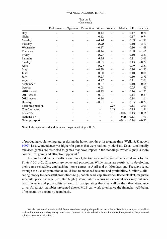
As far as the individual predictor variables are concerned, Table 4 presents the estimatedcomponent weights for each item of the six attendance drivers that was eventually entered into theanalysis. Concerning performance, the Pirates’ winning percentage (WP) had a positive impacton attendance, suggesting that people were more likely to attend when the team was performingwell. In addition, opponents such as the Boston Red Sox, the Detroit Tigers, and the Philadel-phia Phillies appeared to attract higher attendance than the Houston Astros or the WashingtonNationals. What is perhaps most valuable for the Pirates management team are the results forthe 23 promotions. Bobblehead, cap, fireworks, fleece blanket, magnetic schedule, price pack-age (i.e., Buc Night), stein, and t-shirt have significant positive effects on fan attendance; it isalso comforting to note that no promotion significantly decreased attendance. For venue, Fridayand Saturday games were more attractive and games on Monday or Tuesday were less attrac-tive. In addition, July and August appeared to be more attractive than other months, whereasApril was least attractive. School attendance (i.e., summer vacation) may be an important factorhere as well (Lemke et al., 2010). Attendance was also higher with more comfortable weather.Somewhat surprisingly, fan attendance increased with precipitation. Perhaps this was the result

PSYCHOMETRIKA

TABLE 4.Estimated component weights.

Performance Opponent Promotion Venue Weather Media S.E. t-statistic

Pirates WP 0.37 – – – – – 0.14 2.70Pirates 10-game WP −0.06 – – – – – 0.13 −0.43Pirates season WPvs. opponent

0.04 – – – – – 0.13 0.28

GB Pirates 0.23 – – – – – 0.18 1.25ARI – −0.14 – – – – 0.10 −1.44ATL – 0.21 – – – – 0.11 1.91BAL – 0.09 – – – – 0.10 0.86BOS – 0.36 – – – – 0.09 3.98CHC – 0.19 – – – – 0.11 1.81CHW – 0.12 – – – – 0.10 1.22CIN – −0.06 – – – – 0.11 −0.51CLE – 0.19 – – – – 0.13 1.49COL – −0.01 – – – – 0.10 −0.13DET – 0.20 – – – – 0.09 2.11FLA – −0.14 – – – – 0.10 −1.50HOU – −0.36 – – – – 0.12 −3.13KCR – 0.08 – – – – 0.10 0.83LAD – −0.03 – – – – 0.10 −0.32MIL – −0.17 – – – – 0.11 −1.55MIN – 0.04 – – – – 0.09 0.40NYM – 0.04 – – – – 0.10 0.45PHI – 0.40 – – – – 0.10 3.82SDP – 0.08 – – – – 0.10 0.79SFG – −0.08 – – – – 0.10 −0.82STL – −0.12 – – – – 0.11 −1.09WSN – −0.20 – – – – 0.10 −2.03Bobblehead – – 0.26 – – – 0.07 3.73Bottle – – −0.04 – – – 0.07 −0.52Bowl – – −0.01 – – – 0.07 −0.09Canvas wrap/print – – −0.01 – – – 0.08 −0.19Cap – – 0.14 – – – 0.07 2.01Coffee clutch – – 0.00 – – – 0.07 0.07Concert – – 0.09 – – – 0.09 1.01Cooler – – 0.07 – – – 0.08 0.88Figurine/bust – – 0.08 – – – 0.07 1.18Fireworks – – 0.46 – – – 0.11 4.18Fleece blanket – – 0.15 – – – 0.06 2.31Gloves/scarf set – – −0.11 – – – 0.07 −1.68Kids – – 0.12 – – – 0.19 0.63Magnetic schedule – – 0.67 – – – 0.08 8.63Mom – – 0.09 – – – 0.08 1.22Poster/wall calendar – – −0.11 – – – 0.07 −1.49Price package – – 0.35 – – – 0.07 5.03Stein – – 0.28 – – – 0.08 3.58Theme day – – 0.07 – – – 0.07 0.95Tote bag – – 0.12 – – – 0.06 1.84Towel – – 0.00 – – – 0.07 0.07T-shirt – – 0.26 – – – 0.10 2.52Umbrella – – 0.04 – – – 0.07 0.58

WAYNE S. DESARBO ET AL.

TABLE 4.(Continued.)

Performance Opponent Promotion Venue Weather Media S.E. t-statistic

Day – – – 0.12 – – 0.17 0.74Night – – – −0.12 – – 0.17 −0.74Monday – – – −0.18 – – 0.09 −1.97Tuesday – – – −0.20 – – 0.10 −2.10Wednesday – – – −0.17 – – 0.10 −1.69Thursday – – – −0.14 – – 0.08 −1.66Friday – – – 0.27 – – 0.10 2.59Saturday – – – 0.39 – – 0.11 3.61Sunday – – – −0.03 – – 0.13 −0.22April – – – −0.24 – – 0.09 −2.57May – – – −0.20 – – 0.10 −1.92June – – – 0.00 – – 0.10 0.01July – – – 0.27 – – 0.10 2.73August – – – 0.22 – – 0.11 2.03September – – – −0.07 – – 0.10 −0.68October – – – −0.08 – – 0.05 −1.652010 season – – – −0.19 – – 0.14 −1.352011 season – – – 0.03 – – 0.14 0.232012 season – – – 0.16 – – 0.14 1.14Holiday – – – −0.01 – – 0.05 −0.22Total precipitation – – – – 0.27 – 0.13 2.01Comfort index – – – – 0.29 – 0.15 1.96Local TV – – – – – −0.02 0.13 −0.16National TV – – – – – 0.26 0.13 1.99Other pro sport – – – – – −0.14 0.14 −0.95

Note: Estimates in bold and italics are significant at p < 0.05.

of producing cooler temperatures during the hotter months prior to game time (Welki & Zlatoper,1999). Lastly, attendance was higher for games that were nationally televised. Usually, nationallytelevised games are restricted to games that have impact in the standings, which signals a morecompetitive game and attractive opponent.2

In sum, based on the results of our model, the two most influential attendance drivers for thePirates’ 2010–2012 seasons are venue and promotion. While teams are restricted in developingtheir game schedules, emphasizing home games in April and on Mondays and Tuesdays (e.g.,through the use of promotions) could lead to enhanced revenue and profitability. Similarly, allo-cating money to successful promotions (e.g., bobblehead, cap, fireworks, fleece blanket, magneticschedule, price package [i.e., Buc Night], stein, t-shirt) versus unsuccessful ones may enhanceteam revenue and profitability as well. In manipulating these as well as the other attendancedrivers/predictor variables presented above, MLB can work to enhance the financial well-beingof its teams on a team-by-team basis.

2We also estimated a variety of different solutions varying the predictor variables utilized in the analysis as well aswith and without the orthogonality constraints. In terms of model selection heuristics and/or interpretation, the presentedsolution dominated all others.

PSYCHOMETRIKA

TABLE 5.Estimated ERA b coefficients for the six attendance drivers.

Coefficient LB UB

Performance 0.17 0.12 0.38Opponent 0.32 0.27 0.44Promotion 0.51 0.34 0.92Venue 0.60 0.54 1.00Weather 0.10 0.04 0.18Media 0.09 −0.09 0.20

Note: Estimates in bold and italics indicate that the 95 % confidence interval does not contain zero.

6. Comparative Results Obtained from ERA

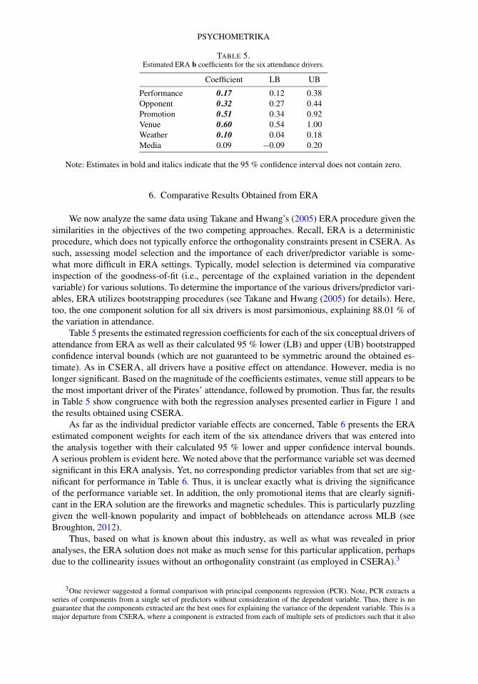
We now analyze the same data using Takane and Hwang’s (2005) ERA procedure given thesimilarities in the objectives of the two competing approaches. Recall, ERA is a deterministicprocedure, which does not typically enforce the orthogonality constraints present in CSERA. Assuch, assessing model selection and the importance of each driver/predictor variable is some-what more difficult in ERA settings. Typically, model selection is determined via comparativeinspection of the goodness-of-fit (i.e., percentage of the explained variation in the dependentvariable) for various solutions. To determine the importance of the various drivers/predictor vari-ables, ERA utilizes bootstrapping procedures (see Takane and Hwang (2005) for details). Here,too, the one component solution for all six drivers is most parsimonious, explaining 88.01 % ofthe variation in attendance.

Table 5 presents the estimated regression coefficients for each of the six conceptual drivers ofattendance from ERA as well as their calculated 95 % lower (LB) and upper (UB) bootstrappedconfidence interval bounds (which are not guaranteed to be symmetric around the obtained es-timate). As in CSERA, all drivers have a positive effect on attendance. However, media is nolonger significant. Based on the magnitude of the coefficients estimates, venue still appears to bethe most important driver of the Pirates’ attendance, followed by promotion. Thus far, the resultsin Table 5 show congruence with both the regression analyses presented earlier in Figure 1 andthe results obtained using CSERA.

As far as the individual predictor variable effects are concerned, Table 6 presents the ERAestimated component weights for each item of the six attendance drivers that was entered intothe analysis together with their calculated 95 % lower and upper confidence interval bounds.A serious problem is evident here. We noted above that the performance variable set was deemedsignificant in this ERA analysis. Yet, no corresponding predictor variables from that set are sig-nificant for performance in Table 6. Thus, it is unclear exactly what is driving the significanceof the performance variable set. In addition, the only promotional items that are clearly signifi-cant in the ERA solution are the fireworks and magnetic schedules. This is particularly puzzlinggiven the well-known popularity and impact of bobbleheads on attendance across MLB (seeBroughton, 2012).

Thus, based on what is known about this industry, as well as what was revealed in prioranalyses, the ERA solution does not make as much sense for this particular application, perhapsdue to the collinearity issues without an orthogonality constraint (as employed in CSERA).3

3One reviewer suggested a formal comparison with principal components regression (PCR). Note, PCR extracts aseries of components from a single set of predictors without consideration of the dependent variable. Thus, there is noguarantee that the components extracted are the best ones for explaining the variance of the dependent variable. This is amajor departure from CSERA, where a component is extracted from each of multiple sets of predictors such that it also

WAYNE S. DESARBO ET AL.

TABLE 6.Estimated ERA component weights.

Performance Opponent Promotion Venue Weather Media LB UB

Pirates WP 0.60 – – – – – −0.75 1.32Pirates 10-game WP −0.10 – – – – – −0.56 0.54Pirates season WPvs. opponent

−0.20 – – – – – −0.79 0.26

GB Pirates 0.61 – – – – – −0.86 1.28ARI – −0.12 – – – – −0.28 0.03ATL – 0.20 – – – – 0.01 0.37BAL – 0.12 – – – – −0.12 0.36BOS – 0.41 – – – – 0.00 0.56CHC – 0.17 – – – – −0.02 0.31CHW – 0.12 – – – – −0.07 0.32CIN – −0.08 – – – – −0.25 0.09CLE – 0.29 – – – – −0.08 0.57COL – −0.03 – – – – −0.22 0.25DET – 0.25 – – – – 0.01 0.41FLA – −0.20 – – – – −0.35 −0.07HOU – −0.36 – – – – −0.55 −0.10KCR – 0.17 – – – – −0.04 0.47LAD – −0.12 – – – – −0.33 0.06MIL – −0.23 – – – – −0.40 −0.03MIN – 0.11 – – – – −0.00 0.28NYM – 0.07 – – – – −0.13 0.18PHI – 0.44 – – – – 0.13 0.56SDP – 0.04 – – – – −0.20 0.30SFG – −0.04 – – – – −0.18 0.15STL – −0.13 – – – – −0.25 0.06WSN – −0.17 – – – – −0.34 0.08Bobblehead – – 0.26 – – – −0.01 0.44Bottle – – 0.00 – – – −0.14 0.07Bowl – – −0.00 – – – −0.06 0.08Canvas wrap/print – – −0.01 – – – −0.25 0.17Cap – – 0.16 – – – −0.04 0.30Coffee clutch – – −0.01 – – – −0.17 0.11Concert – – 0.06 – – – −0.19 0.34Cooler – – 0.04 – – – −0.14 0.15Figurine/bust – – 0.12 – – – −0.10 0.24Fireworks – – 0.47 – – – 0.04 0.74Fleece blanket – – 0.13 – – – −0.00 0.29Gloves/scarf set – – −0.12 – – – −0.28 0.04Kids – – 0.55 – – – −0.38 0.83Magnetic schedule – – 0.64 – – – 0.06 0.86Mom – – 0.11 – – – −0.07 0.27Poster/wall calendar – – −0.09 – – – −0.34 0.07Price package – – 0.30 – – – 0.00 0.64Stein – – 0.23 – – – −0.06 0.47Theme day – – 0.07 – – – −0.08 0.20Tote bag – – 0.10 – – – 0.00 0.17Towel – – 0.02 – – – −0.06 0.11T-shirt – – 0.28 – – – −0.05 0.52Umbrella – – 0.08 – – – −0.01 0.19

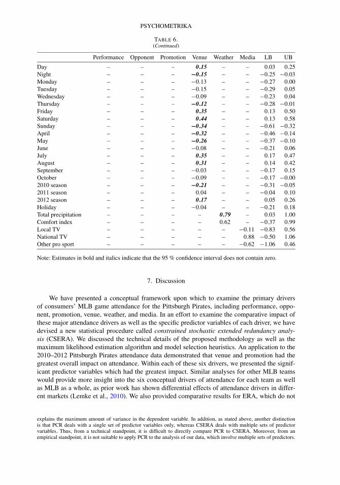
PSYCHOMETRIKA

TABLE 6.(Continued)

Performance Opponent Promotion Venue Weather Media LB UB

Day – – – 0.15 – – 0.03 0.25Night – – – −0.15 – – −0.25 −0.03Monday – – – −0.13 – – −0.27 0.00Tuesday – – – −0.15 – – −0.29 0.05Wednesday – – – −0.09 – – −0.23 0.04Thursday – – – −0.12 – – −0.28 −0.01Friday – – – 0.35 – – 0.13 0.50Saturday – – – 0.44 – – 0.13 0.58Sunday – – – −0.34 – – −0.61 −0.32April – – – −0.32 – – −0.46 −0.14May – – – −0.26 – – −0.37 −0.10June – – – −0.08 – – −0.21 0.06July – – – 0.35 – – 0.17 0.47August – – – 0.31 – – 0.14 0.42September – – – −0.03 – – −0.17 0.15October – – – −0.09 – – −0.17 −0.002010 season – – – −0.21 – – −0.31 −0.052011 season – – – 0.04 – – −0.04 0.102012 season – – – 0.17 – – 0.05 0.26Holiday – – – −0.04 – – −0.21 0.18Total precipitation – – – – 0.79 – 0.03 1.00Comfort index – – – – 0.62 – −0.37 0.99Local TV – – – – – −0.11 −0.83 0.56National TV – – – – – 0.88 −0.50 1.06Other pro sport – – – – – −0.62 −1.06 0.46

Note: Estimates in bold and italics indicate that the 95 % confidence interval does not contain zero.

7. Discussion

We have presented a conceptual framework upon which to examine the primary driversof consumers’ MLB game attendance for the Pittsburgh Pirates, including performance, oppo-nent, promotion, venue, weather, and media. In an effort to examine the comparative impact ofthese major attendance drivers as well as the specific predictor variables of each driver, we havedevised a new statistical procedure called constrained stochastic extended redundancy analy-sis (CSERA). We discussed the technical details of the proposed methodology as well as themaximum likelihood estimation algorithm and model selection heuristics. An application to the2010–2012 Pittsburgh Pirates attendance data demonstrated that venue and promotion had thegreatest overall impact on attendance. Within each of these six drivers, we presented the signif-icant predictor variables which had the greatest impact. Similar analyses for other MLB teamswould provide more insight into the six conceptual drivers of attendance for each team as wellas MLB as a whole, as prior work has shown differential effects of attendance drivers in differ-ent markets (Lemke et al., 2010). We also provided comparative results for ERA, which do not

explains the maximum amount of variance in the dependent variable. In addition, as stated above, another distinctionis that PCR deals with a single set of predictor variables only, whereas CSERA deals with multiple sets of predictorvariables. Thus, from a technical standpoint, it is difficult to directly compare PCR to CSERA. Moreover, from anempirical standpoint, it is not suitable to apply PCR to the analysis of our data, which involve multiple sets of predictors.

WAYNE S. DESARBO ET AL.

display as much face validity compared to the results obtained from CSERA for this particularapplication.

Future research related to CSERA could pursue a number of different directions. First,CSERA could be applied to a wider variety of settings, especially those that contain a large num-ber of collinear explanatory variables and where a priori theory exists on the conceptual driversthat impact the dependent variable(s). Second, while we illustrate the usefulness of CSERA ona problem with one dependent variable and various conceptual drivers, the method can easily beextended to allow for more complex relationships between variables. For example, direct effectsof exogenous variables, higher-order components, and multisample comparisons can readily beincorporated (see Takane & Hwang, 2005). Third, expanding this methodology to cross-sectionalsurvey data would also prove useful in a number of domains. For example, an examination ofcustomer satisfaction or service quality evaluation surveys may provide insight into the respec-tive data structures given that each of these survey applications contains naturally defined de-pendent variables together with theoretical/conceptual drivers—each of which is measured bymultivariate items. A fourth potential methodological extension of CSERA would be to allowfor autocorrelation directly in the likelihood estimation framework to accommodate time seriesapplications and/or to allow for multiple dependent variables, which would be useful for manytypes of multivariate applications. Fifth, given that the dependent variable in this applicationdeals with MLB attendance, theoretically the dependent variable is doubly censored from below(at 0) and above at maximum stadium capacity (seating capacity is 38,362 in the current Piratescontext). While the lower limit is never reached, there are several sell-outs during the season. Assuch, an extension of the existing methodology would be to adjust the likelihood for this censor-ing. Sixth, the development of procedures for variable selection in the CSERA framework wouldprove efficient in identifying the most important subset of predictor variables within each driverset. Finally, predictive validation comparisons with other related procedures such as partial leastsquares (PLS), structural equation models (SEM), extended redundancy analysis (ERA), elasticnets (EN), and inverse regression (IR) would be beneficial for both real empirical data as well assimulated data whose structure was known a priori in order to compare performance.

Acknowledgements

The authors wish to thank three anonymous reviewers and the section editor for their con-structive comments. The authors also wish to thank Frank Coonelly, President of the Pirates, LouDePaoli, Executive Vice President and CMO of the Pirates, Jim Plake, Executive Vice Presidentand CFO of the Pirates, and Jim Alexander, Senior Director of Business Analytics of the Pirates,for their cooperation in the execution of this research.

References

Allan, S. (2004). Satellite television and football attendance: the not so super effect. Applied Economics Letters, 11(2),123–125.

Anderson, T.W. (1951). Estimating linear restrictions on regression coefficients for multivariate normal distributions. TheAnnals of Mathematical Statistics, 22(3), 327–351.

Baade, R.A., & Tiehen, L.J. (1990). An analysis of Major League Baseball attendance, 1969–1987. Journal of Sport &Social Issues, 14(1), 14–32.

Badenhausen, K., Ozanian, M., & Settimi, C. (2013, March 27). MLB team values: the business of baseball. Forbes.Retrieved from http://www.forbes.com/mlb-valuations/list/.

Baimbridge, M., Cameron, S., & Dawson, P. (1996). Satellite television and the demand for football: a whole new ballgame? Scottish Journal of Political Economy, 43(3), 317–333.

Barilla, A.G., Gruben, K., & Levernier, W. (2008). The effect of promotions on attendance at Major League Baseballgames. Journal of Applied Business Research, 24(3), 1–14.

Baseball-Reference.com (2013). Pittsburgh Pirates team history & encyclopedia. Retrieved from http://www.baseball-reference.com/teams/PIT/.

PSYCHOMETRIKA

Becker, M.A., & Suls, J. (1983). Take me out to the ballgame: the effects of objective, social, and temporal performanceinformation on attendance at Major League Baseball games. Journal of Sport Psychology, 5(3), 302–313.

Beckman, E.M., Cai, W., Esrock, R.M., & Lemke, R.J. (2012). Explaining game-to-game ticket sales for Major LeagueBaseball games over time. Journal of Sports Economics, 13(5), 536–553.

Bird, P.J.W.N. (1982). The demand for league football. Applied Economics, 14(6), 637–649.Boyd, T.C., & Krehbiel, T.C. (2003). Promotion timing in Major League Baseball and the stacking effects of factors that

increase game attractiveness. Sport Marketing Quarterly, 12(3), 173–183.Broughton, D. (2012, November 12). Everybody loves bobbleheads: popular giveaway climbs past t-shirts, headwear to

top spot on promotions list. Sports Business Journal. Retrieved from http://www.sportsbusinessdaily.com/Journal/Issues/2012/11/12/Research-and-Ratings/Bobbleheads.aspx.

Carroll, J.D. (1968). Generalizations of canonical correlation to three or more sets of variables. In Proceedings of the76th annual meeting of the American Psychological Association (pp. 227–228).

Davies, P.T., & Tso, M.K.S. (1982). Procedures for reduced-rank regression. Applied Statistics, 31(3), 244–255.DeSarbo, W.S. (2009, December 21). Measuring fan avidity can help marketers narrow their focus. Sports Business Jour-

nal. Retrieved from http://www.sportsbusinessdaily.com/Journal/Issues/2009/12/20091221/From-The-Field-Of/Measuring-Fan-Avidity-Can-Help-Marketers-Narrow-Their-Focus.aspx.

DeSarbo, W.S., Stadler Blank, A., & McKeon, C. (2012, May 14). Proper mix of promotional offerings can producefor teams. Sports Business Journal. Retrieved from http://www.sportsbusinessdaily.com/Journal/Issues/2012/05/14/Opinion/From-the-Field-of-Research.aspx.

Dvorchak, R. (2008, March 30). Losing has lost its luster. Pittsburgh Post-Gazette. Retrieved from http://www.post-gazette.com/stories/sports/pirates/losing-has-lost-its-luster-387105/.

Efron, B. (1982). The jackknife, the bootstrap and other resampling plans (Vol. 38). Philadelphia: SIAM.Efron, B., & Tibshirani, R.J. (1998). An introduction to the bootstrap (Vol. 57). Boca Raton: CRC Press.Fizel, J.L., & Bennett, R.W. (1989). The impact of college football telecasts on college football attendance. Social Science

Quarterly, 70(4), 980–988.Gitter, S.R., & Rhoads, T.A. (2010). Determinants of Minor League Baseball attendance. Journal of Sports Economics,

11(6), 614–628.Green, P.J. (1984). Iteratively reweighted least squares for maximum likelihood estimation, and some robust and resistant

alternatives. Journal of the Royal Statistical Society. Series B. Methodological, 46(2), 149–192.Greenstein, T.N., & Marcum, J.P. (1981). Factors affecting attendance of Major League Baseball: I. Team performance.

Review of Sport & Leisure, 6(2), 21–34.Hansen, H., & Gauthier, R. (1989). Factors affecting attendance at professional sport events. Journal of Sport Manage-

ment, 3(1), 15–32.Hastie, T., Tibshirani, R., & Friedman, J. (2009). The elements of statistical learning: data mining, inference, and pre-

diction (2nd ed.). New York: Springer.Hill, J.R., Madura, J., & Zuber, R.A. (1982). The short run demand for Major League Baseball. Atlantic Economic

Journal, 10(2), 31–35.Hoerl, A.E., & Kennard, R.W. (1970). Ridge regression: applications to nonorthogonal problems. Technometrics, 12(1),

69–82.Hotelling, H. (1936). Relations between two sets of variates. Biometrika, 28(3/4), 321–377.Hwang, H. (2009). Regularized generalized structured component analysis. Psychometrika, 74(3), 517–530.Hwang, H., & Takane, Y. (2004). Generalized structured component analysis. Psychometrika, 69(1), 81–99.Hwang, H., Suk, H.W., Lee, J.H., Moskowitz, D.S., & Lim, J. (2012). Functional extended redundancy analysis. Psy-

chometrika, 77(3), 524–542.Hwang, H., Suk, H.W., Takane, Y., Lee, J.H., & Lim, J. (2013). Generalized functional extended redundancy analysis

(Working paper). McGill University.Izenman, A.J. (1975). Reduced-rank regression for the multivariate linear model. Journal of Multivariate Analysis, 5(2),

248–264.Jöreskog, K.G. (1973). A general method for estimating a linear structural equation system. In A.S. Goldberger & O.D.

Duncan (Eds.), Structural equation models in the social sciences (pp. 85–112). New York: Seminar Press.Kappe, E., Stadler Blank, A., & DeSarbo, W.S. (2014). A general multiple distributed lag framework for estimating the

dynamic effects of promotions. Management Science, fothcoming.Kettenring, J.R. (1971). Canonical analysis of several sets of variables. Biometrika, 58(3), 433–451.Le Cessie, S., & Van Houwelingen, J.C. (1992). Ridge estimators in logistic regression. Applied Statistics, 41(1), 191–

201.Lee, A.H., & Silvapulle, M.J. (1988). Ridge estimation in logistic regression. Communications in Statistics. Simulation

and Computation, 17(4), 1231–1257.Lemke, R.J., Leonard, M., & Tlhokwane, K. (2010). Estimating attendance at Major League Baseball games for the 2007

season. Journal of Sports Economics, 11(3), 316–348.Lohmöller, J.B. (1989). Latent variable path modeling with partial least squares. Heidelberg: Physica-Verlag.Marcum, J.P., & Greenstein, T.N. (1985). Factors affecting attendance of Major League Baseball: II. A within-season

analysis. Sociology of Sport Journal, 2(4), 314–322.McDonald, M., & Rascher, D. (2000). Does bat day make cents? The effect of promotions on the demand for Major

League Baseball. Journal of Sport Management, 14, 8–27.Plunkett Research, Ltd. (2013). Sports industry overview. Retrieved from www.plunkettresearch.com/sports-recreation-

leisure-market-research/industry-statistics.

WAYNE S. DESARBO ET AL.

Ramsay, J.O., & Silverman, B.W. (2005). Functional data analysis (2nd ed.). New York: Springer.Rao, C.R. (1964). The use and interpretation of principal component analysis in applied research. Sankhya: The Indian

Journal of Statistics, Series A, 26(4), 329–358.Reinsel, G.C., & Velu, R.P. (1998). Multivariate reduced-rank regression: theory and applications. New York: Springer.Richards, F.S.G. (1961). A method of maximum-likelihood estimation. Journal of the Royal Statistical Society. Series B.

Methodological, 23(2), 469–475.Siegfried, J.J., & Hinshaw, C.E. (1977). Professional football and the anti-blackout law. Journal of Communication,

27(3), 169–174.Siegfried, J.J., & Hinshaw, C.E. (1979). The effect of lifting television blackouts on professional football no-shows.

Journal of Economics and Business, 32(1), 1–13.Sports Business Journal (2013, May 13). MLB turnstile tracker. Sports Business Journal. Retrieved from http://www.

sportsbusinessdaily.com/Journal/Issues/2013/05/13/Research-and-Ratings/MLB-Turnstile-Tracker.aspx.Takane, Y., & Hwang, H. (2005). An extended redundancy analysis and its applications to two practical examples.

Computational Statistics & Data Analysis, 49(3), 785–808.Trail, G.T., Robinson, M.J., & Kim, Y.K. (2008). Sport consumer behavior: a test for group differences on structural

constraints. Sport Marketing Quarterly, 17(4), 190–200.Van Den Wollenberg, A.L. (1977). Redundancy analysis an alternative for canonical correlation analysis. Psychometrika,

42(2), 207–219.Velu, R.P. (1991). Reduced rank models with two sets of regressors. Applied Statistics, 40(1), 159–170.Wedel, M., & DeSarbo, W.S. (1995). A mixture likelihood approach for generalized linear models. Journal of Classifi-

cation, 12(1), 21–55.Welki, A.M., & Zlatoper, T.J. (1999). U.S. professional football game-day attendance. Atlantic Economic Journal, 27(3),

285–298.Wold, H. (1975). Path models with latent variables: the NIPALS approach. In H.M. Blalock, A. Aganbegian, F.M. Borod-

kin, R. Boudon, & V. Cappecchi (Eds.), Quantitative sociology: international perspectives on mathematical andstatistical modeling (pp. 307–357). New York: Academic Press.

Wold, H. (1982). Soft modeling: the basic design and some extensions. In K.G. Jöreskog & H. Wold (Eds.), Systemsunder indirect observation: causality, structure, prediction (Part II) (pp. 1–54). Amsterdam: North-Holland.

Yee, T.W., & Hastie, T.J. (2003). Reduced-rank vector generalized linear models. Statistical Modelling, 3(1), 15–41.Zhang, J.J., & Smith, D.W. (1997). Impact of broadcasting on the attendance of professional basketball games. Sport

Marketing Quarterly, 6(1), 23–29.

Manuscript Received: 11 MAY 2013