constrained propeller ship noise removal and its ... · constrained propeller ship noise removal...

Constrained propeller ship noise removal and its application to OBC data Manhong Guo*, Jun Cai, Jim Specht, Bin Wang TGS-Nopec Geophysical Company, 2500 CityWest Blvd. Suite 2000, Houston, TX 77042, USA Summary A constrained propeller ship noise removal technique for OBC data has been developed. The constraints include the ship lane information, global linear fitting to determine the ship movement, and the calculation of relative ship locations from different shots. The following field data examples from TGS Cameron SaD Survey demonstrate the effectiveness of the method. Introduction Propeller ship noise can be a serious issue when acquiring seismic data near a commercial shipping lane. It is practically impossible to stop the ships from passing through while acquiring the seismic data. At deep reflection times the propeller ship noise can be stronger than the reflective signal. For this kind of survey environment it is important to suppress the propeller noise while preserving the signal. Manin and Bonnot (1993) proposed the solution which flattened the noise with a static shift by knowing the coordinate of the noise source and travel times and suppressed the noise with existing multi-channel filtering tools. Gulunay et al (2005) proposed to use semblance to automatically locate the static scattering noise source such as shallow sea bed obstructions. Brittan et al (2008) showed another good example by using a similar approach. The Method and Field Data Examples For OBC data, the travel time of the ship propeller noise traveling from the ship to the seismic receiver is where T is the total travel time from ship to the OBC receiver, (Sx, Sy) is ship location coordinates, (Rx, Ry, Rz) is the OBC receiver location coordinates. Vscan is the scanned focusing velocity. Consider the case in which two OBC cables are located near the shipping lane and recording the ship propeller noise. In order to determine the location of the ships we first need to decide where to search. Since we know the ships are traveling within the shipping lane we can limit the search for the ships within the shipping lane. We divide the shipping lane into a grid of cells each with dimensions of

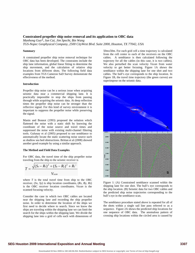
50mx50m. For each grid cell a time trajectory is calculated from the cell center to each of the receivers on the OBC cables. A semblance is then calculated following the trajectory for all the cables (in this case, it is two cables). We also perturbed the scan velocity Vscan from water velocity to get better focusing. Figure 1A shows the semblance within the shipping lane for one shot and two cables. The bull’s eye corresponds to the ship location. In Figure 1B, the travel time trajectory (the green curves) are superimpose on the seismic data.

A

B

scan

zyyxx

V

RRSRST

222 )()( +−+−=

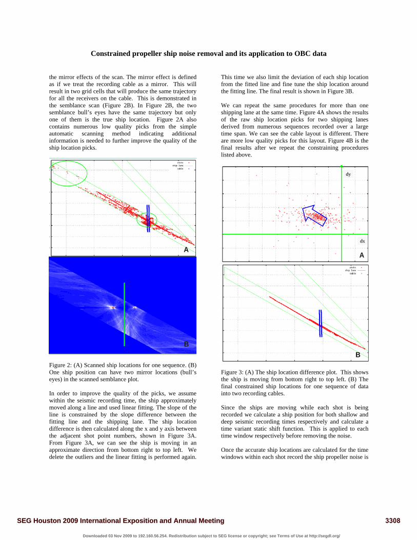
Figure 1: (A) Constrained semblance scanned within the shipping lane for one shot. The bull’s eye corresponds to the ship location. (B) Seismic data for two OBC cables and the predicted ship noise trajectories corresponding to the bull’s eye in the semblance scan. The semblance procedure stated above is repeated for all of the shots within a single sail line pass referred to as a sequence. Figure 2A shows the predicted ship locations for one sequence of OBC data. The anomalous pattern of crossing ship locations within the circled area is caused by

3307SEG Houston 2009 International Exposition and Annual Meeting

Downloaded 03 Nov 2009 to 192.160.56.254. Redistribution subject to SEG license or copyright; see Terms of Use at http://segdl.org/

Constrained propeller ship noise removal and its application to OBC data

the mirror effects of the scan. The mirror effect is defined as if we treat the recording cable as a mirror. This will result in two grid cells that will produce the same trajectory for all the receivers on the cable. This is demonstrated in the semblance scan (Figure 2B). In Figure 2B, the two semblance bull’s eyes have the same trajectory but only one of them is the true ship location. Figure 2A also contains numerous low quality picks from the simple automatic scanning method indicating additional information is needed to further improve the quality of the ship location picks.

A

B

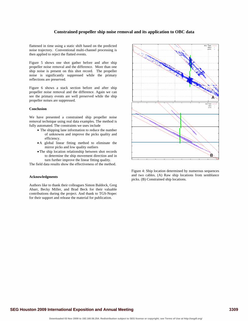
Figure 2: (A) Scanned ship locations for one sequence. (B) One ship position can have two mirror locations (bull’s eyes) in the scanned semblance plot. In order to improve the quality of the picks, we assume within the seismic recording time, the ship approximately moved along a line and used linear fitting. The slope of the line is constrained by the slope difference between the fitting line and the shipping lane. The ship location difference is then calculated along the x and y axis between the adjacent shot point numbers, shown in Figure 3A. From Figure 3A, we can see the ship is moving in an approximate direction from bottom right to top left. We delete the outliers and the linear fitting is performed again.

This time we also limit the deviation of each ship location from the fitted line and fine tune the ship location around the fitting line. The final result is shown in Figure 3B. We can repeat the same procedures for more than one shipping lane at the same time. Figure 4A shows the results of the raw ship location picks for two shipping lanes derived from numerous sequences recorded over a large time span. We can see the cable layout is different. There are more low quality picks for this layout. Figure 4B is the final results after we repeat the constraining procedures listed above.

dy

dx

A

B Figure 3: (A) The ship location difference plot. This shows the ship is moving from bottom right to top left. (B) The final constrained ship locations for one sequence of data into two recording cables. Since the ships are moving while each shot is being recorded we calculate a ship position for both shallow and deep seismic recording times respectively and calculate a time variant static shift function. This is applied to each time window respectively before removing the noise. Once the accurate ship locations are calculated for the time windows within each shot record the ship propeller noise is




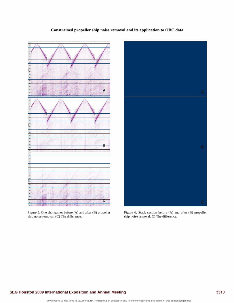
flattened in time using a static shift based on the predicted noise trajectory. Conventional multi-channel processing is then applied to reject the flatted events. Figure 5 shows one shot gather before and after ship propeller noise removal and the difference. More than one ship noise is present on this shot record. The propeller noise is significantly suppressed while the primary reflections are preserved. Figure 6 shows a stack section before and after ship propeller noise removal and the difference. Again we can see the primary events are well preserved while the ship propeller noises are suppressed. Conclusion We have presented a constrained ship propeller noise removal technique using real data examples. The method is fully automated. The constraints we uses include

• The shipping lane information to reduce the number of unknowns and improve the picks quality and efficiency.

• A global linear fitting method to eliminate the mirror picks and low quality outliers

• The ship location relationship between shot records to determine the ship movement direction and in turn further improve the linear fitting quality.

The field data results show the effectiveness of the method. Acknowledgments Authors like to thank their colleagues Simon Baldock, Greg Abarr, Becky Miller, and Brad Beck for their valuable contributions during the project. And thank to TGS-Nopec for their support and release the material for publication.

A

B Figure 4: Ship location determined by numerous sequences and two cables. (A) Raw ship locations from semblance picks. (B) Constrained ship locations.




A

B

C

A

B

C

Figure 5: One shot gather before (A) and after (B) propeller ship noise removal. (C) The difference.

Figure 6: Stack section before (A) and after (B) propeller ship noise removal. C) The difference.



EDITED REFERENCES Note: This reference list is a copy-edited version of the reference list submitted by the author. Reference lists for the 2009 SEG Technical Program Expanded Abstracts have been copy edited so that references provided with the online metadata for each paper will achieve a high degree of linking to cited sources that appear on the Web. REFERENCES Brittan, J., L. Pidsley, D. Cavalin, A. Ryder, and G. Turner, 2008, Optimizing the removal of seismic interference noise: The

Leading Edge, 27, 166–175. Gulunay, N., M. Magesan, and J. Connor, 2005, Diffracted noise attenuation in shallow water 3D marine surveys: 75th Annual

International Meeting, SEG, Expanded Abstracts, 2138–2141. Manin, M., and J. N. Bonnot, 1993, Industrial and seismic noise remove in marine processing: 55th Conference and Exhibition,

EAGE.



constrained propeller ship noise removal and its ... · constrained propeller ship noise removal...

Documents