consequences of firms’ relational financing in...
TRANSCRIPT

53CONSEQUENCES OF FIRMS’ RELATIONAL FINANCING
Journal of Applied Economics, Vol. VIII, No. 1 (May 2005), 53-79
CONSEQUENCES OF FIRMS’ RELATIONALFINANCING IN THE AFTERMATH OF THE 1995
MEXICAN BANKING CRISIS
GONZALO CASTAÑEDA*
Universidad de las Américas-Puebla
Submitted May 2001; accepted May 2004
This paper shows that, in the aftermath of the 1995 banking crisis, relational financing wasa two-edged sword for firms listed on the Mexican Securities Market. On the negativeside, only bank-linked firms observed on average a dependence on cash stock to financetheir investment projects. On the positive side, the banking connection was important toboost their profit rates during the 1997-2000 period, at least for financially healthy firms.These econometric results are derived from dynamic panel data models of investment andprofit rates, which are estimated by the Generalized Method of Moments, where level anddifference equations are combined into a system.
JEL classification codes: L25, D82, N26
Key words: relational financing, banking crisis, internal capital markets
I. Introduction
The Mexican banking crisis provides an interesting case that allows
scrutinizing the impact of relational financing under conditions of financial
turmoil. The Mexican economy experienced a severe banking and currency
crisis in 1995, which practically paralysed the domestic financial system from
1995 to 2000. However, the real annual GDP growth observed in the 1997-
* Castañeda: Departamento de Economía Universidad de las Américas-Puebla, Ex-haciendade Santa Catarina Mártir, Cholula, Puebla, 72820, México, e-mail:[email protected]. This paper was financed with a research grant from UC-MEXUS-CONACYT, whose support I deeply appreciate. I am also very thankful to CarlosIbarra, David Wetzell, a co-editor, and two anonymous referees who read the manuscript andgave me very helpful comments.

54 JOURNAL OF APPLIED ECONOMICS
2000 period was, on average, slightly above 5%, despite that several banks
were intervened and others were sold out due to a huge problem of non-
performing loans and poor capitalization ratios.
Some papers studying this period, like Lederman et al. (2000) and Krueger
and Tornell (1999), have argued that the access of Mexican firms that produce
tradable goods to U.S. financial markets was a key factor in explaining the
recovery after 1995. However, the outstanding performance in the real sector
during the 1997-2000 period would not have been possible without financial
flows from the tradable to the non-tradable sector. In this paper, it is
hypothesized that the existence of business networks and bank ties might
have contributed to the recovery of profits and to the formation of a stronger
internal capital market which made the speedy recovery of the Mexican
economy possible. In particular, the econometric model presented here
analyses: (i) the influence of bank ties on large firms’ profitability before and
during the period of financial paralysis (1995-2000), and (ii) how such linkages
influenced investment decisions.
Babatz (1998), and Gelos and Werner (2002) estimate similar investment
models for the Mexican case, although they analyze a different time period.
In both cases, these authors were concerned with the consequences on the
economy’s real activity when moving towards financial liberalization.1
Therefore, a key contribution of this paper is to test some of the consequences
of relational financing in an emerging economy that enters into a stage of
financial disruption.2
An econometric analysis with bank loans in the 1993-1999 period is
presented by La Porta et al. (2003). These authors find that, after controlling
1 While the latter paper includes also small and medium firms, in the former paper thedataset is based on firms listed in the Mexican Securities Market (BMV, for its Spanishacronym), as it is done here.
2 Castillo (2003) also estimates investment equations for Mexican listed firms in the 1993:I-2001:II period. However, his study suffers from important drawbacks: seasonality inquarterly data is not properly handled; it does not uses GMM estimations and hence theendogeneity problem is not addressed; different regression are run with a split sample, andthus Wald tests for detecting different financial patterns cannot be applied; his models donot consider lagged investment as usually done in dynamic equations. Likewise, the issueof banking ties is not emphasized in his paper.

55CONSEQUENCES OF FIRMS’ RELATIONAL FINANCING
for size, profitability and leverage, related parties received better terms on
average (lower interest rates, less collateral, longer maturities, fewer personal
guarantees) than unrelated parties, despite that the former parties had much
higher default rates and lower recovery rates. The models estimated here
complement their analysis, in so far as the consequences of these practices on
publicly-held firms’ investment in physical capital and profitability are studied.
In the aftermath of the crisis, it is not necessarily the case that the preferential
treatment allowed more access to external financing or higher profits for firms
with bank ties. Thus, the looting suggested in La Porta et al. might simply be
a reflection of wealthier financier-industrialists but poorer and financially
distressed firms.
Theoretically, there is no straightforward prediction as to how relational
financing would alter the impact of the banking crisis on a firm. Banking ties
could have a positive impact on firms’ profitability if the ties enabled the
firms to drain banks’ financial resources. In an integrated financial strategy, a
business network with a financial arm might decide to heavily subsidise the
network’s firms in anticipation of a government bail out program. If,
alternatively, the firms in a business network put their financial health at risk
by trying to rescue their group’s troubled banks, the relational financing would
have a negative impact on profits.
With regard to investment decisions on fixed assets, banking ties are
especially important when there are financial constraints in the economy. In a
normal macroeconomic setting, when the economy moves toward a period of
limited external financing, the financial bottlenecks that exist for firms in
general may not be as strong for firms with banking ties. However, when the
financial stringency is caused, in part, by the fragility of banks’ outstanding
loans, this may result in firms with banking ties having to rely more on their
retained earnings. Firstly, a troubled bank may have difficulties to finance
even their closest firms. Secondly, the international financial markets, who
may be the only source of external funding available, could discount a firms’
link with troubled banks.
Despite that firms with banking ties may experience financial bottlenecks,
these firms can have larger profits relative to ‘independent’ firms, as long as
they do not carry a heavy debt burden. This is so, because the ties will still

56 JOURNAL OF APPLIED ECONOMICS
help to ensure relatively cheap credit for the firms even though its supply has
become more limited; in fact, this is precisely the result observed for the
economic recovery period (1997-2000).
The remaining of the paper is structured as follows. Section II reviews
briefly the literature on relational financing. Section III explains the database
variables and has some descriptive statistics for the investment ratio and profit
returns. Section IV presents the dynamic profit and investment equations, the
econometric methodology and the interpretation of results. Finally, section V
presents the paper’s conclusions.
II. Brief Review of the Literature
Relational financing has been shown to be important for both developed
and emerging economies alike. In the former case, relational credit between
banks and small and medium-sized firms has been useful even when securities
markets are already well-developed, as Petersen and Rajan (1994) and Gande
et al. (1998) show for the United States. A similar situation is presented with
venture capital. This form of external funding is important for start-up firms
engaged in risky activities. Moreover, in earlier stages of economic
development, related banking has been crucial for fostering economic growth,
as described by Hoshi and Kashyap (2001) for the Japanese economy, and by
Lamoreaux (1994) for the United States economy. In all these cases, relational
financing becomes a viable and constructive institution when tacit information
is involved in a borrower-lender relationship.
On the other hand, as emphasized by some authors trying to explain the
1997 East Asian crisis (McKinnon and Pill, 1999; and Rajan and Zingales,
1998), relational financing, when it is based on market power considerations
or policy-induced rents for the financier, can make intermediaries more prone
to moral hazard, soft-budget constraints, and inefficient and unfair crony
capitalism. All in all, these diverse experiences and theories suggest that the
relative benefits of relational financing vis-à-vis arm’s length financing in
terms of efficiency and stability have to do with the macroeconomic setting,
the economy’s judiciary and legal environment, and the firms’ corporate
governance.

57CONSEQUENCES OF FIRMS’ RELATIONAL FINANCING
III. Database and some Descriptive Statistics
A. Database
The database contains a panel of non-financial firms listed on the Mexican
Securities Market (BMV). It has information on balance sheets and income
statements for an unbalanced panel of 176 firms over the 1990-2000 period.3
Each firm in the database has at least four years of information; this is necessary
to have an adequate lag structure for the explanatory variables and their
instruments. In some years, a subset of firms was not quoted on the stock
exchange (even though their information was made public since they issued
bonds or commercial paper in BMV); consequently, Tobin’s Q cannot be
calculated for the entire unbalanced panel. The sample covers two contrasting
periods: financial liberalization (1990-1994) and financial paralysis (1995-
2000); a comparison between the two periods allows testing for whether there
was a structural change during the 1995 banking crisis. The sample also divides
firms into two categories: independent and bank-linked firms. A bank tie
exists when at least one of the firm’s board members belongs to the directorate
of one or more banks.
B. Descriptive Statistics
Firms’ performance with regard to their investment and profitability is
calculated in Tables 1 and 2. Despite the limitations behind a descriptive
analysis, mean values are helpful to detect if there is some tentative evidence
of a pattern change as the economy moves from financial liberalization (1990-
1994) to financial crisis (1995-1996), and then to economic recovery (1997-
2000). Likewise, the possibility of a different financial structure can also be
explored when analyzing mean values according to the type of firm:
3 The precise definition for all the variables is presented in the Appendix. All monetaryvariables are expressed in real terms; the consumer price index used to adjust for inflationis available in the web pages of INEGI and Banco de México. The bank linkage dummyvariable is constructed from the list of boards of directors presented in the Annual FinancialFacts and Figures, published by BMV.

58 JOURNAL OF APPLIED ECONOMICS
independent or bank linked. Both the structural changes through time and the
different behavior according to type are observed in these tables when referring
to the point estimates. However, no statistical validation can be offered in
this exercise; not only because of the need of using control variables to make
inferences but also because standard errors are relatively large.
Table 1. Mean Values for the Investment Ratio
Full sample Refined sample
All firms Bank-linked Indep. All firms Bank-linked Indep.
1991-1994 0.457 0.512 0.345 0.218 0.213 0.229
(4.132) (4.902) (1.678) (0.169) (0.159) (0.188)
1995-1996 0.043 0.030 0.075 0.133 0.126 0.153
(0.228) (0.182) (0.313) (0.120) (0.113) (0.134)
1997-2000 0.161 0.173 0.138 0.153 0.150 0.159
(0.610) (0.730) (0.245) (0.140) (0.141) (0.136)
Notes: Standard errors in parenthesis. Investment ratios are measured as gross investmentto lagged net fixed assets ratio; the refined sample does not include firm-year observationswith zero depreciation, negative investment and investment ratios above 0.75.
Period
With these caveats, it can be observed from Table 1 that the disparity
(standard errors) in investment ratios is specially pronounced in the period of
financial liberalization either for the full sample or for the reduced sample
(where firm-years observations with either negative or extremely large values
are removed). This result might imply that the easy access to financing allowed
some firms to be very aggressive in their expansion strategies, while others
remained conservative; in particular, such disparity is much wider for firms
with banking ties. Moreover, the table shows a cyclical pattern with a sharp
fall in the 1995-1996 period and a slight recovery for the remaining years.
According to point estimates, banking linkage made a difference since the
mean value is higher for firms with bank ties in the 1991-1994 and 1997-
2000 periods in comparison with independent firms when the full sample is
analyzed; however, such a pattern is reversed for the crisis years. In contrast,

59CONSEQUENCES OF FIRMS’ RELATIONAL FINANCING
when referring to the refined sample mean values for ‘independent’ firms
where slightly higher than those observed for bank-linked firms throughout
the sampling period.
Table 2. Mean Values for the Profit Return
Full sample Refined Sample
Period All firms Bank-linked Indep. All firms Bank-linked Indep.
1991-1994 0.025 0.020 0.032 0.065 0.065 0.064
(0.097) (0.101) (0.091) (0.042) (0.040) (0.046)
1995-1996 0.031 0.030 0.033 0.079 0.074 0.088
(0.115) (0.102) (0.138) (0.051) (0.048) (0.056)
1997-2000 0.036 0.030 0.047 0.087 0.081 0.099
(0.209) (0.161) (0.283) (0.178) (0.085) (0.284)
Notes: Standard errors in parenthesis. Profit rates are measured as net earnings to totalassets; the refined sample does not include firm-year observation with negative earnings.
It is shown in Table 2 that standard errors are also very high for the profit
return variable, and that such dispersion increased during the economic
recovery period, in both the full and reduced samples. Although there is not a
substantial difference in the rates of return according to type, mean values
indicate that, in general, independent firms were slightly more profitable.
Moreover, there is no cyclical pattern for these rates like the one observed for
the investment ratios. Profitability increases slightly but steadily over time,
although for bank linked firms the mean profit return is not modified when
moving from crisis to recovery in the sample that includes firms with severe
financial distress. Notice that independent firms in the 1997-2000 period had
the highest average profitability but also that the within group disparities
were very pronounced.
IV. Econometric Equation Models
The Generalized Method of Moments (GMM) introduced by Hansen

60 JOURNAL OF APPLIED ECONOMICS
(1982) is used to estimate the profit and investment equations described below.
The econometric models use a system specification, where equations in levels
and differences are jointly estimated, as suggested by Arellano and Bover
(1995) for dynamic panel models. The econometric literature recognizes the
existence of an endogeneity bias in the estimated coefficients when the
explanatory variables are simultaneously determined with the dependent
variable or when there is a two-way causality relationship. This joint
endogeneity calls for an instrumental variable procedure to obtain consistent
estimates. Therefore, a dynamic GMM technique is attractive since the panel
nature of data allows for the use of lagged values of the endogenous variables
as instruments, as suggested by Arellano and Bond (1991).
Furthermore, a panel data set makes possible to control for firm specific
components of the error term. Firm-specific components represent unobserved
factors whose omission biases the statistical results when using pooled OLS.
In particular, such components are removed when taking first differences in
the regression equation expressed in levels. This in turn removes the need of
additional orthogonality conditions when estimating the coefficients by GMM.
According to Blundell and Bond (1998) the difference estimator has statistical
problems when the dependent and explanatory variables are very persistent
over time. This makes these variables to be weak instruments for the equation
in differences. In this scenario, the system estimator of Arellano and Bover
(1995) can be implemented. An efficient GMM estimator can be achieved
when lagged differences of the endogenous variables are used to instrument
the equation in levels in combination with the level instruments suggested
above for the equation in differences.
A. Profit Equation
A firm’s profits are, in part, the outcome of decision-making based on the
macroeconomic context and the prevailing financial situation in the economy.
This is especially the case once one controls for the idiosyncratic effects of
each firm’s economic activity. Following Lincoln, Gerlach and Ahmadjian
(1996), the model presented below treats firm’s bank ties as an exogenous
component of corporate governance, given the fact that certain business

61CONSEQUENCES OF FIRMS’ RELATIONAL FINANCING
practices of corporate governance can be considered fixed on a short-run
basis. Firms’ profit performance is given by:
where ROAi,t is the return on assets, K
i,t-1 is the stock of fixed assets at the
beginning of the period, Di,t-1
is accumulated liabilities at the beginning of theperiod, Z
i,t is a vector of additional control variables, such as exports to sales
ratio (Xit/NS
it), lagged sales rate of growth (DlnNS
i,t-1) and logarithm of assets
(lnAi,t); f
i is the firm-fixed effects variable, d
t is the time-fixed effects variable,
mi,t is the error term, and DU
i,t is a dummy variable used to capture structural
differences for specific firm-year observations.4 In particular, DUi,t represents
either banking linkages (Bi,t) or years within the financial paralysis period
1995-2000 (Ti,t). The dummy B
i,t takes the value of one if in the year-firm
observation there is a bank link and zero otherwise. A control for a structuralchange in 1995 or 1997-2000 can also be introduced into the above equationwith a year dummy variable T
i,t.
The profit variable used for ROA is measured using net earnings, insteadof operating earnings, in order to capture in the regression the effect of firms’financial operations and banking connections. In equation (1), a positive inertiacoefficient implies that firm’s competitive advantage change slowly over time,regardless of variations in the conditions represented by the other controlvariables.5 In particular, the financial liquidity, organizational capabilities,and network of clients and suppliers, among other things, can guarantee acertain level of profits for the firms.6 By introducing the interaction term
i,t-1i,t 0 1 i,t 2 i,t-1 3 i,t i,t-1 4
i,t-1
DROA + DU + ROA + DU ROA +
Kα α α α α=
5 i,t i t ,+ Z +f +d + i tα µ
(1)
4 Besides controlling for fixed effects at the firm level, the model also takes into considerationfixed effects at the economic sector level.
5 Muller (1986) presents a comprehensive study on profit persistence for US manufacturing
firms.
6 According to the resource-based theory of the firm (Barney, 1991), a competitive advantageis sustained through time because there is heterogeneity across firms in their stock ofresources and their distinctive capabilities, and these two items are scarce and imperfectlymobile. In particular, it is especially difficult for other firms to replicate a firm’s networksof clients and suppliers.

62 JOURNAL OF APPLIED ECONOMICS
Ti,t
x ROA
i,t-1, the model highlights the possibility that the inertia coefficient
changed after the banking crisis. If the estimated coefficient for inertia werereduced, then it would be possible to assert that the firm’s financial operationsand networks may have been disrupted by the banking crisis. On the contrary,should the extent of inertia increase after 1995 then, perhaps, firms were ableto exploit more intensively their liquidity and networks. This would be thecase if firms required their suppliers to finance their working capital expenses,or if firms were able to extract additional rents from clients in an oligopolisticsetting.
The constant term is allowed to be modified for bank-linked firms throughthe use of the dummy variable B
i,t. Thus, if the associated coefficient is positive
it means that, irrespectively of previous profits, these firms were able toundertake certain operations that allowed them to have larger profits incomparison with other firms listed on the BMV. An explanation would be thatrelational banking ties made possible lucrative investment projects by providingthe needed financing or by reducing interest on self-granted loans. This effectwould be independent of the size of the firms’ leverage ratio, which is controlleddirectly by an explanatory variable.
With regard to the control variables, it is predicted that profit rates wouldbe negatively associated with firm’s lagged leverage ratio (D
i,t-1/K
i,t-1)
due to
agency costs. The lagged rate of sales growth (DlnNSi,t-1
) and the log ofcompany’s assets (lnA
i,t) could be both positively associated with profits,
because of either an increase in market power or the exploitation of economiesof scale. Moreover, if domestic demand were constrained then the export tosales ratio would also be positively related with profits.
B. Estimation Results for the Profit Rate Equation Model
The GMM-system estimation results presented in Table 3 have p-valuesthat suggest absence of misspecification for the Sargan test of over-identifying
restrictions, which tests the validity of instruments.7 Furthermore, it can be
7 The level instruments for the difference equation include two, three and four lags, whilethe equation in levels presents only one lagged value for the instruments expressed indifferences. It is important to recall that only the Sargan test based on the two-step GMMestimator is heteroskedasticity-consistent, as pointed out by Arellano and Bond (1991).

63CONSEQUENCES OF FIRMS’ RELATIONAL FINANCING
Table 3. Estimation Results for the Profitability Equation (GMM-System,One-Step Estimation). Dependent Variable: ROAi,t = NPi,t/Ai,t .
(1) (2) (3) (4) (5) (6)
ROAi,t-1
(b1) 0.455*** 0.439*** 0.442*** 0.406*** 0.365*** 1.087***
Ti,t (1995)
ROAi,t-1
0.328*** 0.289*** 0.251*** 0.282*** 0.394*** -0.164***
Ti,t (1997-2000)
ROAi,t-1
(b2) -0.125* -0.106* -0.100 -0.136* -0.294 -0.362***
Bi,t
(b3) 0.011 0.001 0.010 0.008 -0.060 -3.468
Ti,t (1995)
Bi,t
0.003 -0.000 -0.008 -0.002 0.002 0.285
Ti,t (1997-2000)
Bi,t
(b4) 0.029** 0.019* 0.018* 0.026 -0.025 0.119
Di,t-1
/Ki,t-1
-0.001** -0.001*** -0.001** -0.000 -0.002 0.044
Xit/NS
it0.016
DlnNSi,t-1
0.011*
Ln (Ai,t) 0.002
Constant 0.024 0.032** 0.001 0.061 0.067 2.459
No. observations 678 678 678 678 1,098 851
No. firms 133 133 133 133 172 152
Joint Chi-square (P-value) (0.000) (0.000) (0.000) (0.000) (0.000) (0.000)
Sargan test (P-value) (0.999) (0.999) (1.000) (0.998) (0.617) (0.990)
Serial correlation (P-value)
-First order (0.000) (0.000) (0.000) (0.000) (0.001) (0.276)
-Second order (0.530) (0.622) (0.698) (0.475) (0.190) (0.156)
-Third order (0.133) (0.110) (0.141) (0.114) (0.677) (0.326)
Linear restrictions (P-value)
-Ho: b1 + b2 = 0 (0.001) (0.000) (0.000) (0.007) (0.759) (0.000)
-Ho: b3 + b4 = 0 (0.034) (0.273) (0.039) (0.092) (0.597)
Notes: Columns (1-5): NPit = net earnings; column (6): NP
it = operating earnings; column
(4): with sectors. column (5): full sample. Numerical results come from the one-stepcovariance estimators, except the p-value of the Sargan test that corresponds to second-step estimates. Heteroskedasticity corrected standard deviations are used to calculate thep-values (coefficients with p-values up to 0.01, 0.05 and 0.10 are marked by *** , ** and *).The b’s in the first column identify the variables used in the Wald tests. Instruments for thedifference equation (the instruments are included if the variable is present in the modelequations): all variables in levels dated t-2, t-3, t-4. Instruments for the level equation(dummies, and instruments in differences): all variables dated t-1. Series period: 1993-2000, longest time series: 8, shortest time series: 1.

64 JOURNAL OF APPLIED ECONOMICS
seen that there is no persistent serial correlation, and that only first order serial
correlation is not rejected; hence, it can be stated that the models are properly
specified. Results shown in Table 3 come from the one-step estimation, which
yields reliable standard errors.
The profit equation was estimated with the full sample and a refined database
where firm-year observations with negative profits were removed, reducing
the dataset from 1,098 to 678 observations. In a normal macroeconomic context,
the ideal is to use the full sample in order not to reduce the available information.
However, when the economy exhibits such a dramatic shock and there is an
extended period of financial fragility for many firms, it is very difficult to
explain firm’s performance with the profit equation formulated above. Drastic
changes in profits, from a negative to a positive value, can hardly be explained
through inertia and firms’ competencies. As it will be explained below, in the
complex Mexican scenario, some firms were induced to divest and others to
merge in order to improve their financial position. Thus, although both types
of samples were used in the estimations, the results with the refined database
were emphasized since the theoretical literature does not offer a good
understanding of the firm’s strategy in case of severe financial distress.
Therefore, inferences derived from these results are limited to the case of
large firms which are relatively healthy; as a side cost, the understanding of
firm’s performance during this troublesome period is narrowed.
In columns (1) - (4) and (6) the dependent variable includes only firm-
year observations with positive returns on total assets, while in column (5)
the data set includes also firm-year observations with negative profits. Notice
that when the full sample is used, most coefficients are not statistically
significant; although, even in this case, the model is properly specified
according to the GMM procedure for panel data. In this regard, the model
with the reduced sample exhibits a better goodness of fit. In all the results
that use the net earnings ratio as the dependent variable (ROA), included
those that use the full database, the coefficient for the inertia in profits is
positive and increases for the year of the banking crisis (1995), being both
coefficients statistically significant. Moreover, according to the t-statistics
and the Wald tests (Ho: b1 + b
2 = 0) in columns (1), (2), and (4), the inertia
coefficient for the economic recovery period is still positive and statistically
different from zero, but it is lower than the inertia observed for the 1993-

65CONSEQUENCES OF FIRMS’ RELATIONAL FINANCING
1994 period.8 That is, in general, there seems to be a decrease in the level of
inertia for financially healthy firms once the economy entered into the recovery
phase.9
When the banking crisis deepened in 1995, the estimation results show
that listed Mexican firms took advantage of their built-in capabilities, such as
their better access to financial resources and their network of clients and
suppliers. This interpretation is inferred from the fact that most firms listed
on the BMV are large for national standards and are inserted in some form of
business network; thus, these features could have helped these firms to sustain
profits despite the observed depressed demand. Furthermore, the drop in the
inertia coefficient for the profit regression in the 1997-2000 period indicates
that the crisis and the interruption of traditional sources of external financing
in the domestic markets might have handicapped the working of such networks.
Consequently, only on a temporary basis, these firms were capable of taking
advantage of their connections, liquidity and monopoly power to sustain
profitability.
With respect to the differential intercept for firms with banking linkages
Bi,t, there does not appear to be a statistically significant difference in the
levels of profitability for the pre-crisis years and 1995, once adjusted for all
the variables included in the model.10 Nonetheless, the second set of Wald
tests (Ho: b3 + b
4 = 0) presented in columns (1), (3), and (4) indicates that
such linkages were important during the economic recovery period. In other
words, firms with banking ties took advantage of this feature to boost profits,
either because relational financing allowed them to invest in more profitable
projects, or because banks offered some discounts on how much interest was
8 In column (3) the results show no statistical difference for the inertia estimation found inthe 1993-1994 period and that of the 1997-2000 period
.
9 Different time frames were considered for the structural changes in the intercept and the
inertia variable, such as 1993-1994 and 1995-2000 or 1993-1994, 1995-1996, and 1997-2000. Results are not presented here since those models were not properly specifiedaccording to serial correlation tests.
10 A model was also estimated using differentiated intercepts for independent firms in 1995
and in 1997-2000; however, third order serial correlation was detected. Thus, the finalmodel assumes that only for firms with bank ties the intercept can be differentiated alongthe sampling period.

66 JOURNAL OF APPLIED ECONOMICS
charged to the firms; and perhaps for those firms with a debt burden relatively
low, profit returns were even higher that the rates observed in ‘independent’
firms.11
An additional regression is run that uses operating earnings instead of net
earnings in order to confirm whether the changes in the profit inertia were
partially due to the firms’ financial and fiscal operations -see Table 3, column
(6)-. If the coefficients for lagged net and operating earnings were identical,
it would imply that the inertia is caused mainly by the firms’ real operations,
since the former profit variable is defined after taxes and after financial
expenses (or revenues); however, this scenario was discarded by the
estimations.12 The fact that the estimated inertia when using operating earnings
is lower for 1995 than for the pre-crisis years indicates that the human,
organizational and network capabilities of listed firms were not enough per
se to sustain profits during the crisis. On the contrary, the higher coefficient
estimated for that year when using net earnings suggests that these firms had
to rely on financial and/or fiscal strategies to boost their profits. Moreover,
the lack of significance of the debt ratio and bank linkages when using
operating earnings in column (6) shows that these variables influence earnings
not related to the firms’ real operations.13
In summary, this subsection presents important econometric evidence of
two sorts: (i) Firms’ financial strategies were used to shield profits during
11 It is important to clarify that the dataset does not include the bank linkage for those firmswhose associated bank experienced government intervention. As such, the econometricscannot capture properly the influence of extreme cases, where conventional wisdom suggeststhat banks heavily subsidized related firms before being intervened. This feature of thedataset creates a bias against the hypothesis that rates of return might have increased forbank-linked firms during the 1995 crisis.
12 A caveat is in order since the two estimations do not use the exact same sample. Moreover,
the coefficient estimated for the lag of the dependent variable is very close to one whenusing operating earnings, this may imply a unit root problem.
13 The model was also estimated specifying the possibility of a different coefficient for thelagged return on assets, which varies depending on whether firms do or do not have bankinglinkages, and depending also on the time period. Irrespectively of the control variablesused, the model was either not properly specified according to the serial correlation tests,or exhibited a poor goodness of fit as shown by the failure of the Wald tests to reject thehypothesis of no joint significance.

67CONSEQUENCES OF FIRMS’ RELATIONAL FINANCING
1995 through the use of their network of clients and suppliers; however, the
prolongation of the banking and currency crises disrupted such strategies.
(ii) Despite that the leverage ratio is negatively associated with profits, banking
ties resulted helpful in the economic recovery period to boost profits; and
hence the overall impact of the bank linkage on profit returns depends on the
firms’ accumulated debt.
C. Investment Equations
The aim of this subsection is to specify two investment equation models
where the influence of the banking and currency crisis in 1995 is formally
studied. The first is a traditional model used to test whether the significance
of financial restrictions varies over time and across types of firms. The second
model tests whether internal capital markets (based on the pooled cash stock
of firms associated to the same bank) help to explain the weakening of firm-
level financial bottlenecks.14
The Traditional Model
The traditional way to analyze the asymmetric information theory of
investment is to test whether investment in those firms that, a priori, were
considered less affected by asymmetric information problems are less sensitive
to variations in cash stock (or cash flow). Under a normal macroeconomic
setting, firms associated with banks are assumed to face weaker financial
constraints due to the presence of an internal capital market and related credit,
yet this sensitivity results might be reversed under a scenario characterized
by banks’ financial fragility. Furthermore, a larger coefficient for the
investment-cash stock relationship during the 1995-2000 period would be
evidence that a firm’s financial constraints tightened. Investment behavior in
a traditional model is given by:
14 It is common to assume that the estimations from an Euler equation represent a manager’s
rational investment decisions. However, it is still not clear that the typical characterizationof the maximization problem is flawless. Consequently, in this paper it was preferred tofollow a more modest approach by estimating an ad hoc regression equation, which, in anycase, is conventionally used in the literature.
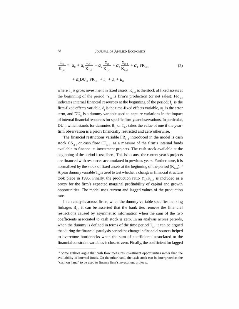
68 JOURNAL OF APPLIED ECONOMICS
where Ii,t is gross investment in fixed assets, K
i,t-1 is the stock of fixed assets at
the beginning of the period, Yi,t is firm’s production (or net sales), FR
i,t-1
indicates internal financial resources at the beginning of the period; fi is the
firm-fixed effects variable, dt is the time-fixed effects variable, m
i,t is the error
term, and DUi,t
is a dummy variable used to capture variations in the impact
of internal financial resources for specific firm-year observations. In particular,
DUi,t, which stands for dummies B
i,t or T
i,t, takes the value of one if the year-
firm observation is a priori financially restricted and zero otherwise.
The financial restrictions variable FRi,t-1
introduced in the model is cash
stock CSi,t-1
or cash flow CFi,t-1
, as a measure of the firm’s internal funds
available to finance its investment projects. The cash stock available at the
beginning of the period is used here. This is because the current year’s projects
are financed with resources accumulated in previous years. Furthermore, it is
normalized by the stock of fixed assets at the beginning of the period (Ki,t-1
).15
A year dummy variable Ti,t
is used to test whether a change in financial structure
took place in 1995. Finally, the production ratio Yi,t/K
i,t-1 is included as a
proxy for the firm’s expected marginal profitability of capital and growth
opportunities. The model uses current and lagged values of the production
rate.
In an analysis across firms, when the dummy variable specifies banking
linkages Bi,t, it can be asserted that the bank ties remove the financial
restrictions caused by asymmetric information when the sum of the two
coefficients associated to cash stock is zero. In an analysis across periods,
when the dummy is defined in terms of the time period Ti,t, it can be argued
that during the financial paralysis period the change in financial sources helped
to overcome bottlenecks when the sum of coefficients associated to the
financial constraint variables is close to zero. Finally, the coefficient for lagged
t,i i,t-1 i,t i,t-10 1 2 3 4 i,t-1
i,t-1 i,t-2 i,t-1 i,t-2
I I Y Y + + + + FR
K K K Kα α α α α=
5 i,t i,t-1 i t i,t + DU FR + f + d + α µ
(2)
15 Some authors argue that cash flow measures investment opportunities rather than theavailability of internal funds. On the other hand, the cash stock can be interpreted as the“cash on hand” to be used to finance firm’s investment projects.
69CONSEQUENCES OF FIRMS’ RELATIONAL FINANCING
investment is expected to be positive but smaller than one, reflecting the inertia
behind adjustment costs in the capital stock.
The Network Model
If, indeed, bank-linked firms’ investments are less sensitive to fluctuations
in their stock of cash then this could be explained by a transfer within a
network formed by all firms associated to the same bank. If there were not
only a bank tie effect but also a network effect, it would follow then that
investment in associate firms should be positively related to the network’s
aggregate resources, and especially to those of cash-rich affiliates.16 As a first
approximation to the problem, all firms with bank ties are considered
constrained, and the sum of cash stocks (flows) from all associate firms
included in the database are assumed to be a potential sources of funding.
From this perspective a network’s cash stock can be transferred toward
investment projects in financially constrained firms. Moreover, this
consolidated cash stock works also as a back-up in case the internally generated
cash in each firm is not enough to service debt obligations. That is, the
network’s cash stock may function as virtual collateral for associate firms,
increasing in that way the willingness of outside lenders to grant additional
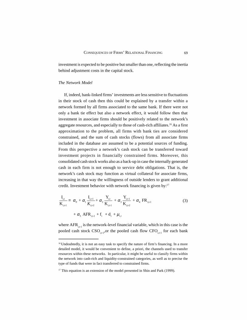
credit. Investment behavior with network financing is given by:17
where AFRi,t-1
is the network-level financial variable, which in this case is the
pooled cash stock CSOi,t-1
,or the pooled cash flow CFOi,t-1
for each bank
16 Undoubtedly, it is not an easy task to specify the nature of firm’s financing. In a moredetailed model, it would be convenient to define, a priori, the channels used to transferresources within these networks. In particular, it might be useful to classify firms withinthe network into cash-rich and liquidity-constrained categories, as well as to precise thetype of funds that were in fact transferred to constrained firms.
17 This equation is an extension of the model presented in Shin and Park (1999).
i,t i,t-1 i,t i,t-10 1 2 3 4 i,t-1
i,t-1 i,t-2 i,t-1 i,t-2
I I Y Y + + + + FR
K K KKα α α α α=
5 i,t-1 i t , + AFR + f + d + i tα µ
(3)

70 JOURNAL OF APPLIED ECONOMICS
network at the beginning of the period (AFRi,t-1
= AFRk,t-1
if k and i belong to
the same network and AFRi,t-1
= 0 if the firm is classified as independent). Inthis exercise, the pooled cash stock is defined by grouping of firms who are
all connected with the same banks.18
Additional extensions to the model are implemented using the same dummy
variables for time period and banking linkage as in model (2). These variablesallow building new interaction terms with both FR and AFR, and then to test
for the influence of banking ties on the sensitivity of firm’s investment tostock of cash, both before and after the banking crisis.
D. Estimation Results for the Investment Rate Equation Models
GMM-system estimation results for investment equations (2) and (3) are
presented in Table 4. These results come from the one-step estimationprocedure, which yields reliable standard errors. All models were run with
the one-year lagged cash flow ratio and the one-year lagged cash stock ratioas proxies for the financial restriction variable; however, the latter ratio showed
a better fit according to the estimated coefficients’ p-values. Therefore, onlyestimations with cash stock are presented. Notice that four sets of regressions
-(1), (3), (4) and (5)- are well specified according to the Sargan and serialcorrelation tests, and diagnostic tests only reject the absence of first order
auto-correlation. The coefficients for the investment rate models presented inthe table, with the exception of column (2), were estimated with a refined
database.In columns (1) and (2), the same simple model was estimated, but with
different samples: while the former estimates use the refined database, thelatter estimates are based on the full sample. In the refined database, firm-
year observations with a negative cash flow ratio were removed, togetherwith those reporting a zero annual depreciation or an investment ratio below
zero or above 0.75.19 Besides the fact that the Sargan test of over-identifying
18 A similar exercise is explored in Castañeda (2003), but using a group membership criteria
based on the interlocking of directorates in non-financial firms.
19 The upper limit was set to exclude those firm-year observations where mergers andacquisitions might have taken place, and which cannot be explained with the traditionalinvestment model. On the contrary, the lower limit excludes those firms who were divesting
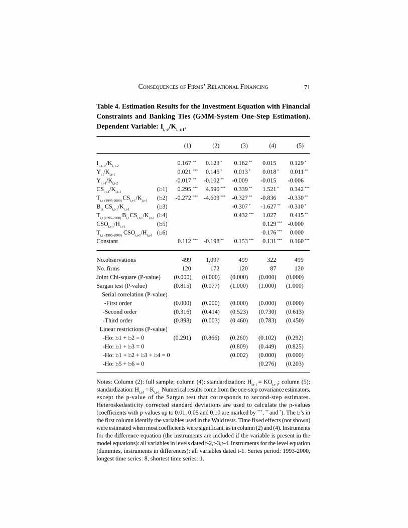
71CONSEQUENCES OF FIRMS’ RELATIONAL FINANCING
Table 4. Estimation Results for the Investment Equation with FinancialConstraints and Banking Ties (GMM-System One-Step Estimation).Dependent Variable: Ii, t//K i, t-1.
(1) (2) (3) (4) (5)
Ii, t-1/
/Ki, t-2
0.167** 0.123* 0.162** 0.015 0.129*
Yi,t/K
i,t-10.021*** 0.145* 0.013* 0.018* 0.011**
Yi,t-1
/Ki,t-2
-0.017** -0.102** -0.009 -0.015 -0.006
CSi,t-1
/Ki,t-1
(b1) 0.295*** 4.590*** 0.339** 1.521* 0.342***
Ti,t (1995-2000)
CSi,t-1
/Ki,t-1
(b2) -0.272*** -4.609*** -0.327** -0.836 -0.330**
Bi,t CS
i,t-1/K
i,t-1(b3) -0.307* -1.627** -0.310*
Ti,t (1995-2000)
Bi,t
CSi,t-1
/Ki,t-1
(b4) 0.432*** 1.027 0.415**
CSOi,t-1
/Hi,t-1
(b5) 0.129*** -0.000
Ti,t (1995-2000)
CSOi,t-1
/Hi,t-1
(b6) -0.176*** 0.000
Constant 0.112*** -0.198** 0.153*** 0.131*** 0.160***
No.observations 499 1,097 499 322 499
No. firms 120 172 120 87 120
Joint Chi-square (P-value) (0.000) (0.000) (0.000) (0.000) (0.000)
Sargan test (P-value) (0.815) (0.077) (1.000) (1.000) (1.000)
Serial correlation (P-value)
-First order (0.000) (0.000) (0.000) (0.000) (0.000)
-Second order (0.316) (0.414) (0.523) (0.730) (0.613)
-Third order (0.898) (0.003) (0.460) (0.783) (0.450)
Linear restrictions (P-value)
-Ho: b1 + b2 = 0 (0.291) (0.866) (0.260) (0.102) (0.292)
-Ho: b1 + b3 = 0 (0.809) (0.449) (0.825)
-Ho: b1 + b2 + b3 + b4 = 0 (0.002) (0.000) (0.000)
-Ho: b5 + b6 = 0 (0.276) (0.203)
Notes: Column (2): full sample; column (4): standardization: Hi,t-1
= KOi,t-1
; column (5):standardization: H
i,t-1 = K
i,t-1. Numerical results come from the one-step covariance estimators,
except the p-value of the Sargan test that corresponds to second-step estimates.Heteroskedasticity corrected standard deviations are used to calculate the p-values(coefficients with p-values up to 0.01, 0.05 and 0.10 are marked by *** , ** and *). The b’s inthe first column identify the variables used in the Wald tests. Time fixed effects (not shown)were estimated when most coefficients were significant, as in column (2) and (4). Instrumentsfor the difference equation (the instruments are included if the variable is present in themodel equations): all variables in levels dated t-2,t-3,t-4. Instruments for the level equation(dummies, instruments in differences): all variables dated t-1. Series period: 1993-2000,longest time series: 8, shortest time series: 1.

72 JOURNAL OF APPLIED ECONOMICS
restrictions for the instruments suggests that the model in column (2) has a
misspecification problem, the high value of the coefficient associated to cash
stock (4.59) is rather surprising.20 In contrast, the same coefficient in column
(1) has a fractional value, as it is traditionally observed in these models.
Undoubtedly, the high sensitivity of investment to cash stock estimated in the
model presented in column (2) is the product of the extreme observations in
the investment ratio.21
Neither the investment equation models used here for analyzing financial
constraints nor those derived from explicit microeconomic foundations are
designed to capture the effects of an aggressive divestment policy, as the one
observed for many firm-years observations in the Mexican case during the
sample period.22 Despite that an intuitive explanation can be offered for such
a high coefficient, it was decided to estimate the remaining models with the
refined database due to a lack of solid theoretical background.23 Obviously,
their fixed assets. In the period of study, there were 28 cases of mergers and acquisitionsfor the firms included in the sample according to news found in different issues of Expansiónmagazine.
20 The same result is obtained when the model uses cash flow instead of cash stock.
.
21 Notice in Table 4, column (2) that the constant coefficient becomes negative when negativeinvestment ratios are included in the sample. This indicates that the estimates associated tothe cash stock variables are heavily influenced by these observations.
22 The number of observation that are lost in the refined database is 598. They are spreadthrough all the sampling period, although there are more observation with a negativeinvestment ratio in the years 1994-1996. Nonetheless, when using time-dummy variablesinteracted with cash stock to differentiate the crises years (1995, 1995-96), the highcoefficient still remains. It is important to recall that the more stringent is the deletioncriteria, the more observations are removed from the unbalanced panel when constructingGMM instruments.
23 Firms experiencing a negative cash flow may decide to reduce their operations and sell
physical assets, either because cash is needed to pay for working capital and financialobligations, or because it has been simply decided to reduce the profile and size of thecompany. There is a multiplying effect because the reduction of one peso in cash stock isassociated with a divestment larger than one. This can be caused by the lumpiness of fixedasset, where the manager is forced to sell assets with a value higher than the financialneeds. Alternatively, a firm reducing its operations may decide to sell sizable physicalassets, perhaps induced by the need to liquidate outstanding debt.

73CONSEQUENCES OF FIRMS’ RELATIONAL FINANCING
this more narrow focus has a cost, since the results can only be interpreted for
large and healthy Mexican firms, missing the possibility of getting a better
understanding of how listed firms in general were able to overcome the crisis.
In column (1) the dummy in the interaction term Ti,t(CS
i,t-1/K
i,t-1) is defined
in terms of the time period 1995-2000, which makes a dynamic interpretation
possible. Notice that all the coefficients are statistically significant and the
sign for the lagged cash stock ratio is positive as suggested by the financial
constraint hypothesis. The most interesting result from this estimation is that
the banking crisis did not exacerbate the financial constraint for the average
firm listed on the BMV, but instead these constraints were removed as
suggested by the Wald test during the 1995-2000 period. This paradoxical
result might be explained by the change in the firms’ financial structure and
the existence of an internal capital market among firms associated to a
particular network. It is possible that the control rights exerted by the parent
company or by affiliates with surplus budgets diminished conflicts of interest
in a lender-borrower relationship, and hence, in a network structure,
information asymmetries were less stringent. Accordingly, the investment-
cash stock sensitivity might have been reduced because listed firms decided
to use their internal capital market more actively since 1995.24
In order to provide a more rigorous test for this statement, the model is
reformulated in column (3) by allowing the interaction term of the financial
restriction to vary across firms and across time, using Bi,t(CS
i,t-1/K
i,t-1) and
Ti,tB
i,t(CS
i,t-1/K
i,t-1). The importance of network membership before 1995 is
evident in column (3), where banking linkages are used as the grouping
criteria. Despite that a policy of financial liberalization was implemented at
the beginning of this sampling period, firms linked to banks through the
interlocking of directorates resulted much less financially constrained than
‘independent’ firms. Additionally, the sum of the corresponding coefficients
was not statistically different from zero according to the Wald test
(Ho: b1 + b
3 = 0). Moreover, the remaining Wald tests show that this situation
24 Similar results are obtained with the full sample -see column (2)-, and thus it cannot be
argued that the reduced cash stock investment sensitivity during financial paralysis is theresult of having only healthy firms, some of them multinationals, with a better access toforeign financing than the remaining firms in the full sample. Moreover, even in the refineddatabase, there was some dependency on cash stock during financial liberalization.

74 JOURNAL OF APPLIED ECONOMICS
was reversed for the 1995-2000 period. While ‘independent’ firms did not
have to rely any longer on retained earnings for their investment projects
(Ho: b1 + b
2 = 0), bank-linked firms had certain dependence on cash stock
since the point estimate of 0.137 was statistically different from zero
(Ho: b1 + b
2 + b
3 + b
4 = 0 is rejected). These econometric results are in line
with the presumption that the banking crisis harmed the financial assessment
of firms with banking ties. As opposed to the ‘independent’ firms, where
financial constraints were removed from 1995 onwards by taking advantage
of international financing, trade or network credit, firms with banking ties
had to rely more on their own resources. A tentative explanation is that for
the latter firms the access to international financing was somewhat limited,
since the market took into consideration the troublesome banking connection,
or alternatively, during this period banks were more heavily scrutinized and
thus were unable to finance investment in linked firms.
The significance of the interaction term with the banking tie dummy in
the first half of the 90’s only implies that these ties were important to reduce
financial constraints. It is not possible to tell whether this result is explained
by the existence of relational credit, or because of the fact that those firms
operate with the support of an internal capital market. Therefore, a more
detailed analysis of the workings of internal capital markets under a bank-
linked network structure is needed to offer a more conclusive answer.
The distinctive feature in the models of columns (4) and (5) in Table 4 is
that they introduce the lagged pooled cash stock CSOi,t-1 for each banking-
group as a proxy for the influence of the internal capital market on the associate
firms’ investment. While in column (4) pooled cash stock is standardized by
the sum of the pooled firms’ capital stock at the beginning of the period
(KOi,t-1
), in column (5), the sum of pooled cash stock is standardized by the
firm’s own capital stock at the beginning of the period (Ki,t-1
). This last
specification assumes that the pool of financial resources available in the
internal capital market should have more influence in the firm’s investment
when that pool is larger relatively to the size of the firm’s physical assets.
Only in column (4) is there evidence of a working internal capital market
for the financial liberalization period since the coefficient on lagged pooled
cash stock CSOi,t-1
/KOt-1
is significantly positive, as expected from theory. It
appears that the aggregated cash stock of firms associated with particular

75CONSEQUENCES OF FIRMS’ RELATIONAL FINANCING
banks helped to spur investment for the average member firm during the
financial liberalization period. Thus, this model presents empirical evidence
that validates the hypothesis of financial relaxation in network firms due to
the workings of an internal capital market built around a banking connection.
However, a Wald test (Ho: b5 + b
6 = 0) rejects the existence of this form of
network-financing during the financial paralysis period. It is also noticeable
that in the latter period, firms with bank ties show –both in columns (4) and
(5)- a positive and statistically significant investment-cash stock sensitivity,
as it was previously indicated with the estimations presented in column (3).
Furthermore, it is important to emphasize that the econometric findings
do not indicate that the internal capital market ceased to exist during the
crisis years. It is possible that exporting firms were issuing international bonds
in order to finance their own investment, as well as the investment of other
firms within the same network; therefore, in this scenario, pooled cash stock
could not be associated to the firm’s investment, despite the use of a network
connection to channel the funds raised abroad. Even if this feature is true, it
needs not to appear in this econometric model since the aggregation of the
data at yearly level -instead of quarterly data- may not be capturing a very
dynamic internal market. Likewise, the internal capital markets prevailing in
the financial paralysis period might have been structured under the basis of
firms’ linkage other than a similar banking connection.
In summary, regression estimates in this subsection show three key results:
(i) There was a structural change during the financial paralysis period in
comparison with the financial liberalization period; however, somewhat
paradoxically, financial constraints were lessened up, at least for ‘independent’
firms. (ii) Before the crisis, bank ties helped to overcome financial bottlenecks,
but after the crisis, financial markets interpreted the bank linkage as a bad
signal on firms’ financial health. (iii) Internal capital markets played,
undoubtedly, a role during the financial liberalization period; however, the
source of the firms’ liquidity during the recovery period remains an open
question.
V. Conclusions
This paper shows that having a banking connection might be a liability

76 JOURNAL OF APPLIED ECONOMICS
for firms in the aftermath of a banking crisis, despite that, traditionally, it has
been argued that bank linkages alleviate financial bottlenecks in normal times.
In the Mexican case, it is observed that limits were imposed to the financing
of investment projects in bank-related firms; however, this shortcoming was
offset, in part, by the positive influence of the bank linkages on firms’
profitability, especially for those firms not carrying a large debt burden from
the financial liberalization period.
Likewise, the paper presents econometric evidence that firms’ financial
operations through their networks of clients and suppliers may be helpful to
boost profit rates on a very short-term basis when a crisis hits the economy.
Yet, the evidence also shows that if such crisis is extended for some years, it
is not longer feasible for large firms to pursue an extraction of rents from
associated firms or other stakeholders. However, the presumption that an
internal capital market acquired a more active role while substituting for
domestic credit financing after 1994 cannot be fully validated with the available
database; thus, two possibilities deserve further exploration to solve this
paradox: incorporating data on international capital markets and making the
use of suppliers’ credit in the estimated equations explicit.
Appendix. Construction and Definition of Variables
It is important to clarify that since 1984 the financial information of firms
listed on the BMV has been re-expressed to reflect the effects of inflation.
Thus, fixed assets, inventories and depreciation are restated by determining
current replacement costs. Moreover, under these accounting principles, a
firm adjusts the value of the debt due to inflation, despite that new debt has
not been granted. For this study, the firms’ balance sheet, income, and cash
flow statements for the 1990-2000 sample period are expressed in real terms
using prices of 2000. The 176 firms of the unbalanced panel add up to 1,460
year-firm observations.
A. Definition of Variables
Iit = Gross investment = K
it – K
i,t-1 + DEP
it, where DEP
it is annual
depreciation; Kit = Net capital stock; Y
it = Production; NS
it = Net sales;
77CONSEQUENCES OF FIRMS’ RELATIONAL FINANCING
FRit = Financial restrictions variables CF
it, CS
it; CF
it = Cash flow; CS
it = Cash
stock; AFRit = Group level financial restriction CSO
it, CFO
it; CSO
it = Pooled
cash stock; CFOit = Pooled cash flow; KO
it = Pooled capital stock; X
it/NS
it
= Exports to sales ratio, where Xit is foreign sales; ROA
it = Return on assets
= NPit/A
it, where NP
it is net profits and A
it is total assets; D
it = Total
liabilities; DUit = Dummy variables to partition the sample according to
liquidity constraints Bit, T
it; B
it = Dummy for banking linkages; T
it = Time
dummy for financial paralysis period (1995 or economic recovery period).
B. Construction of Variables from Primary Sources
Codes: (SIVA; Infosel): Kit = Net capital stock: net assets in plant,
equipment and real estate, valued at current replacement cost (S12; 1,150);
NSit = Net sales (R01; 1,238); Y
it = Production: Net sales minus decrease in
inventories (RO1-C19; 1,238-1,312); Xit = Net foreign sales (R22; 1,262);
DEPit = Depreciation: depreciation and amortization of year t (C13; 1,305);
CSit = Cash stock: cash and temporary investments (S03; 1,141); CF
it = Cash
flow: cash generated from operations (C05; 1,293). This is equal to net income
plus capital amortization and depreciation, plus increase in pension reserves,
minus the increase in receivables, minus the increase in inventories, plus the
increase in payables, plus the increase in mercantile credit; NPit = Net earnings
(R18; 1,255), or operating earnings (R05; 1,242); Ait = Total assets (S01;
1,139); Dit = Total liabilities (S20; 1,159); CSO
it = Pooled cash stock is built
with the summation of the cash stock of the other firms that are linked to the
same bank; CFOit = Pooled cash flow is built with the summation of the
cash flow of the other firms that are linked to the same bank; KOit = Pooled
capital stock is built with the summation of the net fixed assets of the other
firms that are linked to the same bank; Bit = Dummy for banking linkages:
assigns a value of one if the firm has a banking linkage and a value of zero
otherwise. Criteria for banking linkages: A firm is linked with a bank if at
least one of its board members sits on the board of a bank; Tit = Time dummy
for financial paralysis period: assigns a value of one for 1995 and onwards
and a value of zero otherwise.

78 JOURNAL OF APPLIED ECONOMICS
References
Arellano, Manuel, and Stephen R. Bond (1991), “Some Tests of Specification
for Panel Data: Monte Carlo Evidence and Applications to Employment
Equations,” Review of Economic Studies 58: 277-97.
Arellano, Manuel, and Olympia Bover (1995), “Another Look at the
Instrumental Variable Estimation of Error-components Models,” Journal
of Econometrics 68: 29-51.
Babatz, Guillermo (1998), “The Effects of Financial Liberalization on the
Capital Structure and Investment Decisions of Firms: Evidence from
Mexican Panel Data,” unpublished manuscript, México, Secretaría de
Hacienda y Crédito Público.
Barney, Jay B. (1991), “Firm Resources and Sustained Competitive
Advantage,” Journal of Management 17: 99-120.
Blundell, Richard, and Stephen R. Bond (1998), “Initial Conditions and
Moment Restrictions in Dynamic Panel Data Models,” Journal of
Econometrics 87: 115-43.
Castañeda, Gonzalo (2003), “Internal Capital Markets and the Financing
Choices of Mexican Firms, 1995-2000,” in A. Galindo and F. Schiantarelli,
eds., Credit Constraints and Investment in Latin America, Washington
D.C., Inter American Development Bank.
Castillo, Ramón A. (2003), “Las Restricciones de Liquidez, el Canal de Crédito
y la Inversión en México,” El Trimestre Económico 60: 315-42.
Gande, Amir, Manju Puri, Anthony Saunders, and Ingo Walter (1997) “Bank
Underwriting of Debt Securities: Modern Evidence,” Review of Financial
Studies 10: 1175-1202.
Gelos, Gastón R., and Alejandro M. Werner (2002), “Financial Liberalization,
Credit Constraints, and Collateral: Investment in the Mexican
Manufacturing Sector,” Journal of Development Economics 67: 1-27.
Hansen, Lars P. (1982), “Large Sample Properties of Generalized Method of
Moments Estimators,” Econometrica 50: 1029-54.
Hoshi, Takeo, and Anil K. Kashyap (2001), Corporate Financing and
Governance in Japan. The Road to the Future, Cambridge, MA, and
London, MIT Press.

79CONSEQUENCES OF FIRMS’ RELATIONAL FINANCING
Krueger, Anne O., and Tornell, Aarón (1999), “The Role of Bank
Restructuring in Recovering from Crisis: Mexico 1995-98,” Working Paper
7042, Cambridge, MA, NBER.
Lamoreaux, Naomi R. (1994), “Insider Lending: Banks, Personal Connections,
and Economic Development in Industrial New England,” New York,
Cambridge University Press.
La Porta, Rafael, Florencio López-de-Silanes, and Guillermo Zamarripa
(2003), “Related Lending,” Quarterly Journal of Economics 118: 231-
68.
Lederman, Daniel, Ana M. Méndez, Guillermo Perry, and Joseph Stiglitz
(2000), “Mexico: Five Years after the Crisis,” unpublished manuscript,
Washington D.C., World Bank.
Lincoln, James R., Michael L. Gerlach, and Christina L. Ahmadjian (1996),
“Keiretsu Networks and Corporate Performance in Japan,” American
Sociological Review 61: 67-88.
Mckinnon, Ronald I., and Huw Pill (1999), “Exchange-rate Regimes for
Emerging Markets: Moral Hazard and International Overborrowing,”
Oxford Review of Economic Policy 15: 19-38.
Mueller, Dennis C. (1986), Profits in the Long Run, New York, Cambridge
University Press.
Petersen, Mitchell A., and Raghuram G. Rajan (1994), “Benefits from Lending
Relationship: Evidence from Small Business Data,” Journal of Finance
49: 3-37.
Rajan, Raghuram G., and Luigi Zingales (1998), “Which Capitalism? Lessons
from the East Asian Crisis,” Journal of Applied Corporate Finance 11:
40-48.
Shin, Hyun-Han, and Young S. Park, (1999), “Financing Constraints and
Internal Capital Markets: Evidence from Korean Chaebols,” Journal of
Corporate Finance 5: 169-91.