conformance tests for real-time systems with timed automata specifications
TRANSCRIPT
Formal Aspects of Computing (2000) 12: 350–371c© 2000 BCS Formal Aspects
of Computing
Conformance Tests for Real-Time Systemswith Timed Automata SpecificationsRachel Cardell-OliverDepartment of Computer Science, University of Essex, UK
Abstract. A method is introduced for testing the conformance of implemented real-time systems to timedautomata specifications. Uppaal timed automata are transformed into testable timed transition systems (TTTSs)using a test view. Fault hypotheses and a test generation algorithm for TTTSs are defined. Results of applyingthe method are presented.
Keywords: Conformance testing; Real-time systems; Timed automata; Test selection
1. Introduction
The development of real-time systems has been advanced in recent years by new theories and tools fortheir specification and analysis. The language of timed automata [AlD94] is one of the most widely usedfor analysing real-time systems. Automatic verification, simulation and a graphical interface for constructingtimed automata specifications is provided by tools such as Uppaal, Kronos and HyTech. However, althoughwe now know how to analyse the correctness of specifications of real-time systems, down to the level offormal models of programs and machines, we still know little about the problem of whether a physicalimplementation of a real-time system satisfies its specification: that is, how to test an implemented real-timesystem. This paper addresses the problem of conformance testing for real-time systems and proposes a method,using Uppaal timed automata specifications, for generating and managing tests.
The goal of conformance testing is to deduce whether an implementation conforms to its formal spec-ification by performing experiments on the implementation. A fundamental assumption is that experimentson a physical real-time system, here sequences of time stamped input and output events, can be associatedwith traces of the formal specification, in this case traces of Uppaal timed automata. However, the standardsemantics of timed automata [JLS00, LPW97] present several problems for testing.
First, timed automata have a dense time model and so their traces include behaviour which can not beobserved in an experiment. For example, events may be specified to occur at different, but arbitrarily closetimes, leading to different outcomes. However, to an observer the ordering of two arbitrarily close events cannot be distinguished, and a tester does not have sufficient control over a physical system to offer inputs atarbitrarily close, but different times. A more appropriate model for observing real-time systems is a digitalclock approximation [HMP92].
Correspondence and offprint requests to: Rachel Cardell-Oliver, Department of Computer Science, University of Essex, ColchesterCO4 3SQ, UK. Email: [email protected] URL: http://cswww.essex.ac.uk/Research/FSS/people/cardr-hp.html

Testing Real-Time Systems 351
Testable
TTS
Test View
Test GenerationAlgorithm
Test Suite
Test ExecutionHarness
Verdict:YES I conforms to S
or NO I fails test t
Specification
Uppaal
Timed Automata
View Transformation
Fig. 1. Summary of the conformance test method for real-time systems.
Secondly, because Uppaal timed automata differ from I/O automata in having persistent data variables,clocks, and closed world specifications, assumptions underlying test generation methods for I/O automataneeded revising for timed automata. In particular, for real-time systems we introduce new assumptionsregarding state identification, input enabling and extra implementation states.
A final problem is one of scale. Real-time systems are typically specified by a network of communicating,sequential timed automata. The number of possible traces, and hence of test experiments, for such specificationsis very large, if not infinite. The problem of large numbers of test cases is already well known in softwareengineering, and there are established techniques for structuring the test process in which testing is organisedhierarchically into unit, integration and system tests, and tests are grouped according to their particular testpurpose [Pfl98]. This paper shows how these techniques can be applied for conformance testing of real-timesystems. We demonstrate that careful selection of different views for testing a specification is a key to solvingthe problem of too many tests.
This paper presents a test generation method for real-time systems. A standard timed transition systemmodel of a network of Uppaal timed automata is transformed under a given test view into a testable timedtransition system (TTTS). The test view captures information about a particular set of tests: the selection ofrelevant events to be observed; the mapping between implementation and specification events; the granularityof the observer’s clock; a partition of test events into inputs and outputs. By choosing different test views,the tester can control the number of tests required: more detailed tests can be used for critical test purposes,and less detailed tests elsewhere. A test generation algorithm is presented which constructs a set of test casesfrom a TTTS. The resulting test suite is input to a test execution harness for the implementation under test.It is assumed that the implementation can be viewed as a TTTS and that it has no more states than thespecification TTTS. The final output of the test method is a verdict: yes, the implementation conforms toits specification or no, the implementation fails to conform to the specification because it fails a particularexperiment. A summary of this conformance test method is given in Figure 1.
The main contribution of this paper is a test method for real-time systems which provides,
1. test views to capture testing assumptions and give the tester control over the size of test suites,
2. a model, testable timed transition systems (TTTS), for timed automata with persistent data variables;TTTS models provide the basis for test generation,
3. fault hypotheses and a conformance test algorithm for TTTSs.
An algorithm for generating complete test suites for finite state Mealy automata was first proposed by Chowin 1978 [Cho78]. Extensions of Chow’s algorithm for untimed systems have been widely studied [Cho78,Hol91, LBP94, TaP98]. The algorithm has been extended for non-deterministic Mealy automata by Luo,Bochmann and Petrenko [LBP94] and for finite state machines without paired inputs and outputs by Tanand Petrenko [TaP98].
Recently, the application of Chow’s algorithm to real-time systems has been studied. En-Nouaary etal. [EDK98] transform timed input-output automata (TIOA) into non-deterministic timed FSMs for testgeneration. The problem of dense time in TIOA is addressed by using a grid automata over a regiongraph with a given time granularity. Springintveld et al. [SVD99] present a grid algorithm for boundedtime-domain automata which accurately captures real-time behaviours using finitely many points. However,although exact, their grid method is impractical because it generates “an astronomically large number of test

352 R. Cardell-Oliver
sequences” [SVD99]. Cardell-Oliver and Glover present a conformance test method for a discrete time modelof Henzinger’s timed transition systems [CaG98].
The test method of this paper differs from previous methods for real-time systems because its specificationsare a class of Uppaal timed automata. Significantly, Uppaal TAs have persistent data variables, and to thebest of our knowledge our conformance test algorithm is the first to deal with persistent variables. We alsoextend previous methods by introducing test views to manage different levels of detail for testing.
All the above test generation algorithms are complete in that they demonstrate the equivalence of animplementation and its formal specification. An alternative solution to the problem of too many tests isprovided by partial test methods. These give an algorithm for generating any possible test case and from thosethe tester selects samples. The Trio method [MMM95] generates such tests for specifications in temporallogic. Higashino et al. [HNT99] give an algorithm which checks whether a selected timed experiment is acomputation of a given timed automata. Clarke and Lee [ClL95] use domain methods to select boundary timepoints from requirements expressed by events constrained by time intervals. Partial test generators are alsoused for testing reactive systems modelled by events and refusals [Tre96, PeS97]. The VVT approach has beenapplied to real-time systems by including clock resets and timeouts as CSP events in a specification [SMH99].Braberman et al. [BFM97] introduce a time reachability tree to define test cases from high level timed petri nets.
The paper is organised as follows. Section 2 introduces the language of Uppaal timed automata used inthis paper, and recalls their timed transition system semantics. Section 3 describes the different elements of atest view and explains how the timed transition system of an Uppaal specification is transformed, using a testview, into a testable timed transition system (TTTS). Our fault hypotheses and a test generation algorithmfor TTTSs are defined in Section 4. A case study is presented in Section 5 to illustrate test generation for anumber of different test views. The study was performed using Uppaal [Upp99] and the Essex real-time testgeneration tool [Glo00]. A fully worked example of test generation for a simple timed automata specificationis given in the Appendix.
2. Uppaal Timed Automata
In this paper, real-time systems are modelled by timed automata extended with shared data variables andsynchronous communication over channels. Systems are specified as networks of non-deterministic, sequentialprocesses. For convenience we have used the syntax and semantics of timed automata used in the Uppaalsystem [Upp99]. A tutorial introduction to Uppaal is given in [LPW97].
2.1. Timed Transition Systems
Timed transition systems define the behaviour of Uppaal specifications [JLS00]. In the following, D denotesa dense time domain, such as the rationals, Z the integers, N the natural numbers and B the booleans. ATis the set of events possible for timed transition system T.
Definition 2.1. A timed transition system (TTS) is a triple, T = (S, s0,−→) for a set of states S , an initialstate s0 ∈ S and a labelled transition relation, −→⊆ S × (AT ∪ D) × S which satisfies the following three
constraints on its timed transitions: Time determinism: If s1δ−→ s2 and s1
δ−→ s3 then s2 = s3. Time Additivity:
If s1δ1−→ s2 and s2
δ2−→ s3 then s1δ1+δ2−→ s3. Zero Delay: s
0−→ s.
The traces of a TTS are the sequences of events which it can perform. Traces may be finite or infinitesequences.
Definition 2.2. For a timed transition system T = (S, s0,−→), and state s ∈ S , we define 〈e1, e2, . . . , en〉 ∈tracesof(s) for ei ∈ AT ∪ D exactly when there exist si ∈ S such that s
e1−→ s1e2−→ s2 . . . sn−1
en−→ sn. Forinfinite traces, 〈e1, e2, e3, . . .〉 ∈ tracesof(s) exactly when there exists a countably infinite sequence of states andtransitions with labels ei from state s. The traces of the full TTS are simply all possible traces from its initialstate: traces T = tracesof(s0) Trace concatenation is written t1.t2 and the operator is overloaded for sets oftraces: T1.T2 = {t1.t2 | t1 ∈ T1 ∧ t2 ∈ T2}.

Testing Real-Time Systems 353
2.2. Uppaal Input Language
In Uppaal, TTSs are described syntactically by a network of communicating timed automata with location,data and clock variables and synchronisation over named channels. A real-time system is specified bya network of non-deterministic, sequential automata. Each automaton processes p is defined by a set oftransitions Transof(p). The transition set of the specification is the union of the transition sets for each of itsprocesses. In addition a specification assigns initial values to all integer variables and clocks are initialised to0. Transitions have three-part labels. We write:
©i g a r−→ ©jSource i and destination j are control locations of process p. The transition’s guard, g, is a conjunction
of constraints on clocks and data variables. For example, x > 3 ∧ x 6 10 ∧ pos = 20. A set of assignmentsr, resets variables: clock variables can be reset to integer constants and data variables can be reset tointeger expressions. For example, a transition may have the reset set {x := 0, pos := pos + 1}. All variablesare initialised to integer values. For testing, all data variables must have finite domains as in Uppaal, andadditionally clocks must be finitely bounded, being reset if the upper bound is reached. We extend Uppaalsyntax by allowing clocks to be turned off when not required, written x := −1. A synchronisation actioninvolves two transitions, taken simultaneously. One transition offers the synchronisation event, a! and theother event a?. The time which can elapse whilst control remains at any particular control location of aprocess is constrained by location invariants: clock constraints which govern every outgoing transition fromthat location. For testing purposes, clock constraints in both guards and invariants must be closed (that is,using 6,>,= but not < or >: see Section 3.2).
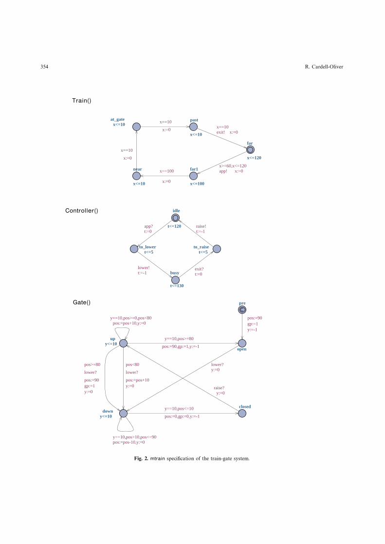
Figure 2 shows a typical timed automata specification of the well known train-gate system. Three processes,a train, a controller and a gate, interact to ensure the safe passage of trains through a level crossing. Trainsapproaching and leaving the crossing are detected by sensors app and exit. The control process reacts tothese signals by sending instructions lower and raise to the gate process. Initially the gate is fully raised(pos==90). Upon receiving a request to lower the gate, the position of the gate is lowered by 10 degrees every10 time units until it is closed (pos==0). Similarly, if a request is received to raise the gate then its position israised by 10 degrees every 10 time units until the gate is fully open. The variable gp is set to 1 when the gatebecomes fully raised, and to 0 when the gate becomes fully lowered. After one train has entered and left thecrossing another train may approach before the gate is fully raised. If this happens, a worst case assumptionis made about the current position of the gate (pos:=pos+10) and lowering resumes. Initial locations foreach process have a double ring and transitions from a location annotated C must be taken immediately thelocation is entered.
2.3. From Uppaal Specification to TTS
An Uppaal specification is characterised by a TTS and a location invariant function Inv. The signature of theTTS is Σ = (P , V , Cl, Ch) where P is the set of process names used, V the set of data variables, Cl the clockvariables and Ch the synchronisation channels. The data variables V include a special location variable, locp,for each process, p ∈ P , of the specification.
The states of the underlying TTS map each data variable in the signature to an integer value and eachclock variable to a value in the time domain D.
S ⊆ (V →Z) ∪ (Cl → D)
A transition of process p with source location i and guard g is enabled in a state s when the process hasreached its initial location and its guard is satisfied.
Enabled (p, i, g) sdef= s(locp) = i ∧ g(s)
The set of events AT of TTS T with signature Σ are triples containing a process name, a (possibly null)synchronisation event in Ch∗ = Ch ∪ {ε}, and a reset set of assignments to persistent variables. A reset set,which may be empty, assigns integer expressions to variables and integer constants to clocks. Once the state
354 R. Cardell-Oliver
at_gatex<=10
far
x<=120
far1
x<=100
near
x<=10
past
x<=10
x==10
x:=0
x>=60,x<=120x:=0app!x==100
x:=0
x==10
x:=0
x==10x:=0exit!
Train()
busy
t<=130
idle
t<=120
to_lowert<=5
to_raiset<=5
t:=0exit?
t:=0app?
t:=-1lower!
t:=-1raise!
Controller()
closeddown
y<=10
open
pre
upy<=10
y:=0raise?
y==10,pos<=10
pos:=0,gp:=0,y:=-1
y==10,pos>10,pos<=90pos:=pos-10,y:=0
y:=0lower?
pos:=90gp:=1y:=-1
pos<80
pos:=pos+10y:=0
lower?
pos>=80
pos:=90gp:=1y:=0
lower?
y==10,pos>=80
pos:=90,gp:=1,y:=-1
y==10,pos>=0,pos<80pos:=pos+10,y:=0
Gate()
Fig. 2. mtrain specification of the train-gate system.

Testing Real-Time Systems 355
context s ∈ S of a reset set r is known, then each integer expression e : S → Z in r can be replaced with aconstant n = e(s). In the following, bold font r is used for this evaluated version of a reset set r.
rdef= {(v, n) | ((v, e) ∈ r ∧ v ∈ V ∧ n = e(s)) ∨ ((v, n) ∈ r ∧ v ∈ Cl)}
When a transition is taken, the new state resulting from the assignment actions is calculated from theassignments in the evaluated reset set. A frame condition states that all variables and clocks which are notexplicitly updated, maintain their current value.
Update s rdef= λ v. if (v, n) ∈ r then n else s(v)
s⊕ δ denotes the state produced by adding δ to the value of each clock variable, and leaving unchangedall location and data variables and any sleeping clocks. The value of δ may be any rational in D not just anatural number as for clock resets.
s⊕ δ def= λ c. if c ∈ Cl ∧ s(c) > 0 then s(c) + δ else s(c)
Clock invariants for each process location are specified by Inv : S → B, a conjunction of state predicatesof the form λ s. s(locp) = li =⇒ s(x) 6 n for each location li of process p ∈ P for clocks x and non-negativeinteger constants n.
An Uppaal specification can now be described by a TTS (S, s0, ◦−−−→), invariant function Inv with Inv(s0)true, signature (P , V , Cl, Ch) and a transition relation defined as follows.
sp ε R◦−−−→ s′ iff ∃ i, j, g, r.
©i g ε r−→ ©j ∈ Transof(P )∧ p ∈ P∧ Enabled (p, i, g) s∧ R = (r ∪ {(locp, j)})∧ s′ = Update s R
sp a R◦−−−→ s′ iff ∃ i, j, g, r, a, k, l, g′, r′, q.
©i g a! r−→ ©j ∈ Transof(p) ∧©k g′ a? r′−→ ©l ∈ Transof(q)∧ p ∈ P ∧ q ∈ P∧ Enabled (p, i, g) s ∧ Enabled (q, k, g′) s∧ R = r ∪ r′ ∪ {(locp, j), (locq, l)}∧ s′ = Update s R
sδ◦−−−→ s′ iff s′ = s⊕ δ ∧ Inv(s′)
Uppaal automata may be non-deterministic in that two transitions from the same location need not havemutually exclusive guards. In general, it is known that non-deterministic timed automata can not be madedeterministic [AFH94]. However, the TTS for an Uppaal specification is deterministic as an FSM, in thatthere can be no two transitions from a reachable state which have the same delay or event label but differentdestination states.
3. Test Views
A fundamental assumption underlying conformance testing is that experiments on a physical real-time systemcan be associated with traces of a formal specification. However, we shall show that the TTS traces of Uppaaltimed automata specifications include some traces which can not be observed and thus can not be used astest experiments. Further, the observable TTS traces do not contain sufficient information to be used as testexperiments. In this section we show how to transform a TTS into a testable TTS (TTTS) which is suitablefor generating test cases.
A test plan describes all the different tests which will be performed on an implemented computersystem [Pfl98]. The plan typically includes unit tests to test individual processes, integration tests to ensure
356 R. Cardell-Oliver
that groups of processes interact correctly, and system tests which check that the full system meets both itsfunctional and performance requirements. A test plan is structured as a collection of different test purposes,usually described in prose. In our framework, each test purpose is documented by an Uppaal specificationand a test view. The parameters of a test view serve to:
• distinguish the system under test from its test environment,
• define a digital clock for observing test experiments,
• define which events are to be observed in the test, either explicitly or implicitly, and which events arehidden or ignored.
A testable timed transition systems (TTTS) is a TTS (SS, s0, •−−−→) derived from the TTS (S, s0, ◦−−−→)with s0 ∈ SS ⊆ S and signature (P , V , Cl, Ch) for both. TTS transition labels are either delays d ∈ D or timedevent triples (p, a, r) with p ∈ P and a ∈ Ch∗ and r ∈ (V ×Z)∪ (Cl×Z). The labels of TTTSs are timed event4-tuples, (d, io, a, r) with discrete delay d ∈ N, input or output label io ∈ {inp, out} and a and r as before.
3.1. Distinguishing between System and Environment
When testing an implemented real-time system it is necessary to distinguish between the test environment andthe system under test in order to interpret a trace as a test experiment. Environment processes provide testinput events, and system processes respond with test outputs.
Partitioning the Uppaal processes of the specification into those of the test environment and those of thesystem under test gives P = E ∪S ∧ E ∩S = ∅. Each TTS transition labelled (Q a r) has a correspondingTTTS transition: if Q ∈ E then the TTTS transition is labelled (0 inp a r) and if Q ∈ S then (0 out a r). Fortransitions involving a synchronisation action. we take the view that the process performing the α! “owns”the synchronisation. Since this distinction is not significant in Uppaal, specifiers need to be aware of it whenwriting specifications which will be used for test generation.
In the mtrain specification of Figure 2 which consists of three processes, Train, Controller and Gate, thepartition E = {Train,Gate} and S = {Controller} describes a unit test of the implemented controller process.In this view, app, exit are test inputs and lower and raise are test outputs. For testing responses of the gate,a partition E = {Train,Controller} and S = {Gate} is used and here lower and raise are test inputs andassignments to pos are test outputs.
3.2. The Observer’s Digital Clock
In the specification language of timed automata, activity is governed by analogue clocks which record timein real number values. This model is suitable for formal analysis, including model checking, but not forrecording physical observations in a test experiment. For example, a tester can not cause events to be offeredat arbitrarily close times but lead to different outcomes [SVD99].
The problem of finding a representative coarse grained model of a dense time system has been widelystudied since such models are useful for simplifying verification problems [Yov95, HMP92, RaS97] as well asfor testing [EDK98, SVD99]. A coarse grained model is defined by a grid which covers the underlying densetime space and maps points of that space onto a single representative of each grid region. In [EDK98] gridsizes for TIOA specifications are proposed, depending on the number of clocks n in the specification. A gridof size 1/2 is sufficient for 1 clock, and 1/(n+ 2) for n > 1 clocks. In [SVD99] a very fine clock grain of 2−n isproposed where n depends not only on the number of clocks but also on the number of states of the transitionsystem representation. The TIOA models used in both [EDK98] and [SVD99] allow clock constraints ofthe form x < n, x > n as well as x = n, x 6 n and x > n. However, since we have already assumed that atester is not be able to control or observe distinctions between x < n and x = n, we restrict our attentionto Uppaal specifications which use only clock constraints related by 6,> and =. In practice, most Uppaalspecifications respect this restriction in any case [Upp99]. Under these constraints Uppaal timed automataare digitisable and it follows from Henzinger, Manna and Pnueli’s digitisation theorem that an integer digitalclock is sufficient to distinguish all TTSs which are distinguishable in the dense time domain [HMP92]. Thedigital clock grain chosen is usually one, but a clock grain equal to any common divisor of all the timebounds used in the specification would be sufficient.
In order to digitise a TTS, each timed trace with times in D is mapped onto a set of possible integer-timed

Testing Real-Time Systems 357
trace interpretations, one for each possible origin ε ∈ [0, 1). For each such ε, every global real time, t ∈ D ismapped to i ∈ Z where i = bxc if x 6 bxc+ ε and i = dxe if x > bxc+ ε. The resulting integer-timed tracegives a coarse-grained view of any real-time sequence of actions. Consider a real-time trace in which eventa at global time 1.2 is followed by b at 2.25 and then c at 2.8. Using a digital clock with time grain 1 andorigin ε = 0, the same sequence of actions is recorded as observing events a, b, c at global times 2,3,3. For timegrain 1 and ε = 0.3 the sequence is recorded as observing a, b, c at global times 1,2,3. The digital model of adense-time TTS includes all possible digitisations of its traces.
The following algorithm for constructing a digitised TTTS has been implemented in the Essex testtool [Glo00]. Start at global time 0 in state s0. Suppose that for a reachable state s in the TTS, event e canoccur after any delay d ∈ D with L 6 d 6 U. For each integer dd ∈ {L, L + 1, . . . , U} we include a TTTStransition from s to sdd with delay dd and event e. Repeat this step for each new state sdd reached until nonew states are created.
Digitising a specification imposes a single time grain over the whole TTS. It is sometimes also useful tovary the grain locally. This effect can be achieved by selecting representative times from an interval and anexample is given in Section 5.2.2.
3.3. Visible and Hidden Events
To test an implementation against a specification we need to relate observable events of the implementationto events of the specification, and hide irrelevant information. A useful side-effect is that hiding usuallyreduces significantly the number of tests required to establish conformance. There are three stages in selectingobservable events.
First, identify implementation outputs of interest for the current test purpose and associate each withan event in the specification: a synchronisation, assignments to certain variables or both. Output events areperformed by taking transitions of system processes.
Second, identify input events which are necessary in order to prompt the outputs of interest. For example,if an output transition’s guard reads the value of some variable, then all environment transitions which assignvalues to that variable must be made visible. Also, if the output process synchronises with the environmentbefore performing the action of interest, then that synchronisation channel should be made visible.
The third class of visible events are implicitly rather than explicitly visible. These events do not correspondto physical events of the tester’s world. However, since the tester has complete control of the environment,every environment action is implicitly visible, including changes of location, clock readings and resets. Thisinformation can be used to simplify testing.
The visible events of a TTTS are defined by a triple V = (V ′, Ch′, Cl′) of subsets of the TTTS signaturesets: V ′ ⊆ V , Ch′ ⊆ Ch and Cl′ ⊆ Cl. The transitions of the TTTS are constructed by mapping a functionVis V over the label of every transition in the TTTS. Equality on visible variables defines an equivalenceclass on states.
Vis V sdef= if s ∈ Ch′ then s else ε
Vis V rdef= {(v, n) | (v, n) ∈ r ∧ v ∈ V ′ ∪ Cl′}
s =V tdef= ∀v. v ∈ (V ′ ∪ Cl′) =⇒ s(v) = t(v)
3.4. TTTS Normal Form
After performing the transformations of the previous sections we get TTTSs containing, for example,
s0(0,inp,a1 ,r1)•−−−→ s1
(d1 ,inp,ε,{})•−−−→ s2(d2 ,out,a2 ,r2)•−−−→ s3 and s1
(d2 ,inp,ε,{})•−−−→ s4(d1 ,out,a2 ,r2)•−−−→ s5
for states si, synchronisations ai, resets ri and delays di. The traces of s0, for example, are not suitable astest experiments because they contain some events which can not be observed for certain. For example, in(d1, inp, ε, {}) there is no visible event to observe after delay d1 so the tester can not know know whetherthe implementation matches the specification’s delay, or is deadlocked, or performing some other task. Tomake events positively observable, each delay step should be matched with a terminating observable event.

358 R. Cardell-Oliver
We make traces observable by eliding empty events with their following visible events. The examples abovebecome,
s0(0,inp,a1 ,r1)•−−−→ s1
(d1+d2 ,out,a2 ,r2)•−−−→ s3 and s1(d2+d1 ,out,a2 ,r2)•−−−→ s5
Performing these simplifications makes some states of the original TTS unreachable (e.g. s2) and it alsomay introduce non-determinacy to the TTTS: two or more edges with the same label from the same state (e.g.the two transitions from s1). Eliding edges can actually increase the number of edges in the TTTS, since for astate with m incoming edges labelled by hidden events and n outgoing edges labelled with visible events, theTTTS before hiding has n+m edges and after hiding has n ∗m edges. Fortunately, in practice eliding usuallyreduces the number of edges (see for example Table 3). If the TTS contains a cycle of edges whose events arehidden, then eliding them would introduce unbounded non-determinism. This situation is not permitted andis flagged by our tool. The problem can be avoided by making visible at least one of the events in the cycle.
Since eliding edges may introduce non-determinism, we normalise the elided TTTS using the classicalalgorithm for transforming a non-deterministic FSM into a deterministic one [HoU79, Glo00]. The resultingTTTS is deterministic as an FSM, but observably non-deterministic from a testing perspective since any statecan have one or more outgoing output edges with different timed event labels, meaning that the system undertest or environment may perform any one of those output events on any run of the system. The TTTS is,however, guaranteed to have bounded observable non-determinism, since
• the original Uppaal TA must have finite domains for all data variables,
• each clock is required to have a finite upper bound enforced by clock guards, location invariants andclock resets,
• digitisation ensures that the set of possible delays from a bounded interval is finite, and
• eliding a cycle of invisible edges is not allowed.
The resulting TTTSs may not be minimal since there may be two or more states in the same visibleequivalence class which have the same set of traces. In this case all but one of those states is redundantin the TTTS. The Essex test tool detects redundant states and performs the necessary renamings using thestandard minimisation algorithm for FSMs [Hol91, Glo00]. This final minimisation step is computationallyexpensive and it has been claimed that minimisation is not essential for complete testing [SVD99]. However,minimisation can provide a substantial reduction in graph size and so we have found it practical to minimisegraphs before generating tests. Some effects of determinising and minimising TTTSs for different views canbe seen in Table 3. The Appendix contains a fully worked example of transforming an Uppaal specificationunder a given view into its corresponding TTTS.
4. Generating Test Suites
TTTSs define a class of real-time specifications whose traces can be interpreted as test experiments. Eachexperiment generated from Spec and passed by Impl provides some evidence that traces(Spec) ⊆ traces(Impl).However, we would like to show more than this: that the implementation has no traces which do not alsobelong to the specification, that is traces(Impl) ⊆ traces(Spec). It is, in fact, possible to construct a finite setof tests, Test(Spec), which proves that traces(Spec) = traces(Impl), if all test cases are passed.
In our test suites, each trace is paired with an oracle which states whether the final timed event should,or should not be observed in the current run. An implementation, modelled by TTTS Impl, passes a test caset ∗ yes when t ∈ traces(Impl) and passes t ∗ no when t 6∈ traces(Impl) but t minus its final event is in Impl.Otherwise, Impl fails the test. We write t ∗ R ∈o traces(Impl) when the test is passed.
In general, we can only show that Impl has no “bad” traces given explicit assumptions about which“bad” implementations are possible. A Fault Hypothesis defines all possible good and bad implementations,Conf(Spec) and Nonconf(Spec). A conformance test generation method is correct if, Impl ∈ Conf(Spec) ∨Impl ∈ NonConf(Spec) =⇒ traces(Spec) = traces(Impl) ⇐⇒ Test(Spec)⊆otraces(Impl). This proposition isproved for our test method in Theorem 4.2.
Testing Real-Time Systems 359
4.1. Fault Hypothesis
The conformance relation for TTTSs is trace equivalence. Since TTTSs are deterministic finite state machines,trace equivalent models are also bisimilar.
Conf(Spec)def= {S | traces(Spec) = traces(S)}
We could have used a weaker conformance relation such as trace inclusion. However we have not done sosince the same effect can be achieved by modifying the original Uppaal specification (see Section 5.2.2) andthis has the advantage of providing a record of exactly what assumptions are made in the tests undertaken,which trace inclusion does not.
Non-conforming implementations are defined in the standard way in terms of possible faults on singletransitions, with multiple faults defined as a sequence of implementations with single faults.
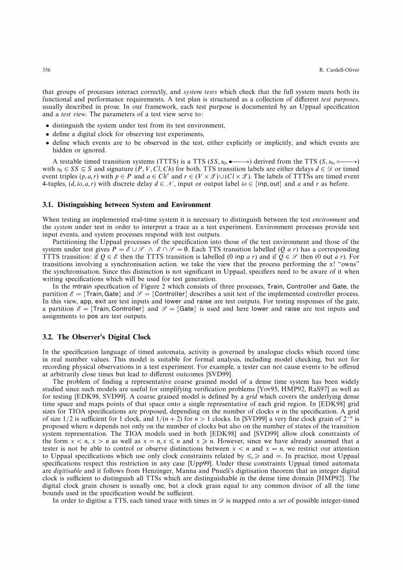
Definition 4.1 (Real-Time Faults). Impl ∈ NonConf(Spec) if and only if
1. Impl has no more states than Spec and
2. Impl has a single transition fault or Impl can be transformed to Spec by a sequence of single transitionfaults.
Impl has a single transition fault for τ = sd m a r•−−−→ s′ ∈ Spec if there is a τ′ = s
d′ m a′ r′•−−−→ s′′ ∈ Impl such thatexactly one of the following holds.
2.1 τ′ has an action fault : Spec− {τ} = Impl − {τ′} ∧ m = out ∧(d 6= d′ ∨ a 6= a′ ∨ r 6= r′)
2.2 τ′ has a transfer fault : Spec− {τ} = Impl − {τ′} ∧ m ∈ {in, out}d = d′ ∧ a = a′ ∧ r = r′∧s′ 6= s′′ ∧ s′ =V s′′
2.3 Impl has an extra transition : Spec ∪ {τ′} = Impl ∧ m = outτ′ /∈ Spec
2.4 Impl has a missing transition : Impl ∪ {τ} = Spec ∧ m = outτ /∈ Impl
4.2. Test Execution Assumptions
In general, if a system under test behaves differently on different runs then experiments are not repeatablebecause a test which is passed on one occasion may fail on another. Even if every test is passed we neverknow whether the system under test might perform differently on another occasion. Any test method for suchsystems would fail the fundamental requirement of repeatability for scientific experiments. However, we needa test method for non-deterministic systems since non-determinism arises naturally in real-time systems: ifan output action may occur at any time during an interval, then we can not usually predict in advance atwhich time the action will occur. In order to test observably non-deterministic systems, we require that givena bounded number of runs of the system, all possible different output responses will be observed. This iscalled the all weathers assumption [LBP94].
A test trace is tester controlled if for each state visited within the trace, the TTTS has no more than oneoutput transition from that state. Tester controlled traces are useful for testing because the implementationcan be forced to execute them, since it has no choice of outputs at any point. In general, however, TTTStraces are system controlled meaning that the implementation may make an output choice not in the trace.By the all weathers assumption, we know that a system controlled trace will eventually be observed, givensufficient runs of the system but some traces may not be observed for a long time. So it is convenient tocalculate all possible candidate traces when there is no tester controlled one so that the tester can use anyobserved trace which is suitable.
Finally, after each successfully completed test, it must be possible to reset the implementation under testto its initial state. A reset can be achieved by a special event which returns the implementation to its initial
360 R. Cardell-Oliver
state (e.g.. reboot or terminate and restart), usually taking a certain amount of time to do so. Alternatively,if the TTTS is a strongly connected graph then a reset can be achieved by extending the current experimenttrace until the initial state is revisited.
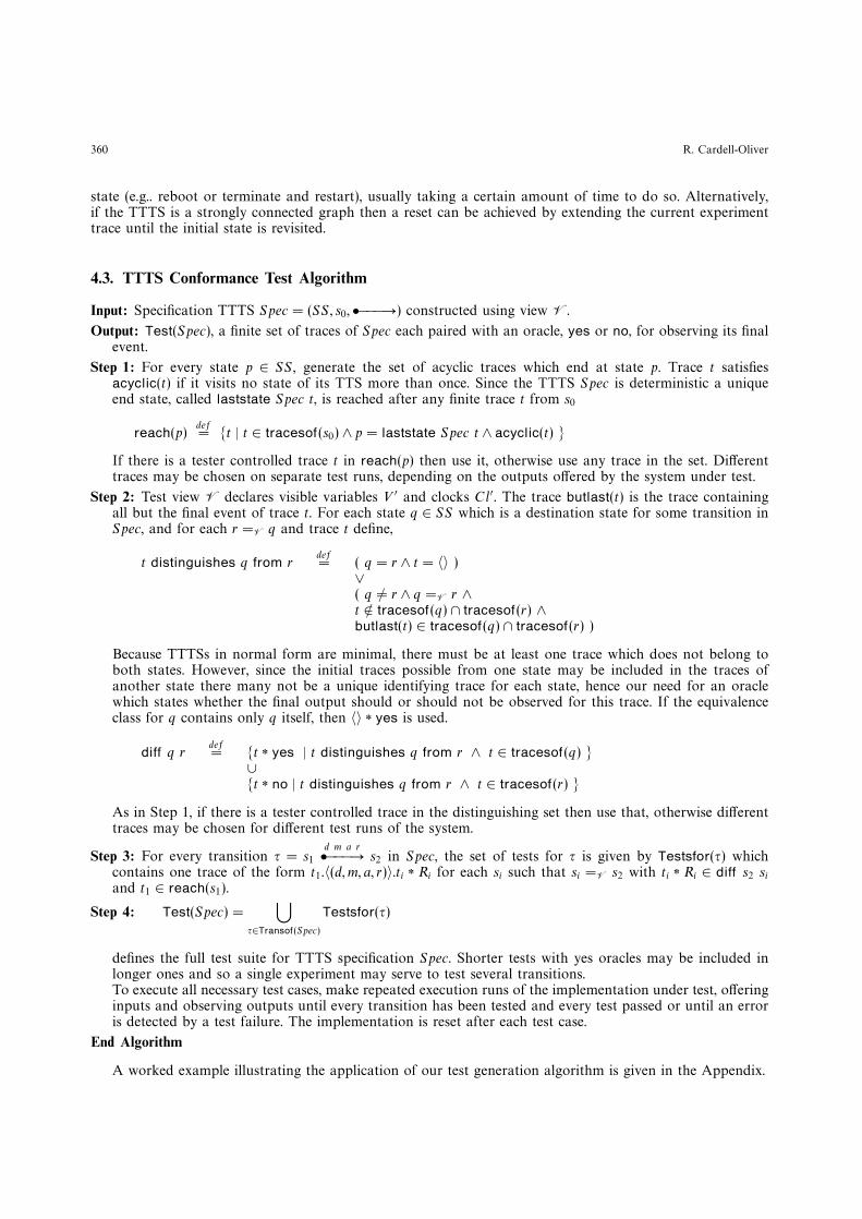
4.3. TTTS Conformance Test Algorithm
Input: Specification TTTS Spec = (SS, s0, •−−−→) constructed using view V.
Output: Test(Spec), a finite set of traces of Spec each paired with an oracle, yes or no, for observing its finalevent.
Step 1: For every state p ∈ SS , generate the set of acyclic traces which end at state p. Trace t satisfiesacyclic(t) if it visits no state of its TTS more than once. Since the TTTS Spec is deterministic a uniqueend state, called laststate Spec t, is reached after any finite trace t from s0
reach(p)def= {t | t ∈ tracesof(s0) ∧ p = laststate Spec t ∧ acyclic(t) }
If there is a tester controlled trace t in reach(p) then use it, otherwise use any trace in the set. Differenttraces may be chosen on separate test runs, depending on the outputs offered by the system under test.
Step 2: Test view V declares visible variables V ′ and clocks Cl′. The trace butlast(t) is the trace containingall but the final event of trace t. For each state q ∈ SS which is a destination state for some transition inSpec, and for each r =V q and trace t define,
t distinguishes q from rdef= ( q = r ∧ t = 〈〉 )
∨( q 6= r ∧ q =V r ∧t 6∈ tracesof(q) ∩ tracesof(r) ∧butlast(t) ∈ tracesof(q) ∩ tracesof(r) )
Because TTTSs in normal form are minimal, there must be at least one trace which does not belong toboth states. However, since the initial traces possible from one state may be included in the traces ofanother state there many not be a unique identifying trace for each state, hence our need for an oraclewhich states whether the final output should or should not be observed for this trace. If the equivalenceclass for q contains only q itself, then 〈〉 ∗ yes is used.
diff q rdef= {t ∗ yes | t distinguishes q from r ∧ t ∈ tracesof(q) }
∪{t ∗ no | t distinguishes q from r ∧ t ∈ tracesof(r) }
As in Step 1, if there is a tester controlled trace in the distinguishing set then use that, otherwise differenttraces may be chosen for different test runs of the system.
Step 3: For every transition τ = s1d m a r•−−−→ s2 in Spec, the set of tests for τ is given by Testsfor(τ) which
contains one trace of the form t1.〈(d, m, a, r)〉.ti ∗ Ri for each si such that si =V s2 with ti ∗ Ri ∈ diff s2 siand t1 ∈ reach(s1).
Step 4: Test(Spec) =⋃
τ∈Transof(Spec)
Testsfor(τ)
defines the full test suite for TTTS specification Spec. Shorter tests with yes oracles may be included inlonger ones and so a single experiment may serve to test several transitions.To execute all necessary test cases, make repeated execution runs of the implementation under test, offeringinputs and observing outputs until every transition has been tested and every test passed or until an erroris detected by a test failure. The implementation is reset after each test case.
End Algorithm
A worked example illustrating the application of our test generation algorithm is given in the Appendix.
Testing Real-Time Systems 361
4.4. Fault Detection Properties of the Algorithm
Theorem 4.1. For TTTS specification Spec, the test suite Test(Spec) generated by the TTTS Test GenerationAlgorithm detects any Impl ∈ Nonconf(Spec).
Proof. If Impl ∈ Nonconf(Spec) then it has at least one single transition fault. We show that for any (thefirst) such fault there is a test case in the test suite which will detect it.
1. If Impl has an action fault then there is a τ′ ∈ Impl with bad output label l′ and corresponding τ ∈ Specwith label l. Every test t1.〈l〉.t2 ∗ R ∈ Testsfor(τ) fails at event l′ since:
• If d′ 6= d then the event will be observed at the wrong time: either early or not within delay d.
• If s′ 6= s ∨ r′ 6= r then since visible synchronisations and assignments of output events correspondto physical events of the implementation under test, the wrong physical event will be output by thesystem under test, and the error detected on some run of the system.
2. If Impl has a transfer fault then there is a τ′ ∈ Impl with bad output destination state s′ and correspondingτ ∈ Spec with destination state s. We know s′ =V s because the same sequence of timed events reached eachstate and all states of Impl are also states of Spec. Therefore, there is a test t1.〈l〉.t2 ∗ R ∈o Testfor(τ) forwhich t2 distinguishes s from s′ and which will be failed by the implementation on the final distinguishingoutput event.
3. If Impl has a missing transition, then after executing the implementation under all weather conditions,there will be no observed test from Testfor(τ) and so the test suite is not complete and the fault will bedetected.
4. If Impl has an extra transition from state s, then in some run of the implementation, a new output eventl′ will be observed when testing the transitions from s. This will be detected as an action error from s.
q
Theorem 4.2 (Test Completeness). If Impl satisfies the test hypotheses then all tests for Spec will be passedby Impl iff Impl is trace equivalent to Spec:
Impl ∈ Conf(Spec) ∨ Impl ∈ NonConf(Spec) =⇒traces(Spec) = traces(Impl) ⇐⇒ Test(Spec)⊆otraces(Impl)
Proof. If Impl ∈ Conf(Spec) then by definition traces(Spec) = traces(Impl) and we also have, as required,that Test(Spec)⊆otraces(Spec) = traces(Impl)
If Impl ∈ Nonconf(Spec) then
traces(Spec) 6= traces(Impl)
By Theorem 4.1 there is a test in Test(Spec) which is failed by Impl. For this reason we have, as required,that
Test(Spec) 6⊆otraces(Impl)
q
4.5. Comparison with Previous Conformance Test Methods
The test framework in this paper differs from previous frameworks [Cho78, LBP94, TaP98, EDK98, SVD99]for I/O automata and TIOA. In particular, TTTS specifications have persistent variables whilst specificationlanguages such as TIOA do not. In this section we highlight some consequences of the differences betweenspecification languages.
4.5.1. State Identification
At any point in the test process we know which state has been reached in the specification TTTS becauseTTTSs are deterministic FSMs. An important problem for conformance algorithms is to determine whetherthe implementation under test has reached an equivalent state. In specification languages without persistent

362 R. Cardell-Oliver
state variables this judgement can only be made on the basis of the traces possible from the reached state.States are identified by executing sufficient traces to distinguish each state from any other in the automaton.This is an expensive part of test generation for I/O automata and TIOA. For TTTS specifications, however,states need only be distinguished from other states in their visible equivalence class. In practice, only a smallpercentage of all possible pairs of TTTS states need be distinguished by a trace as can be seen by comparingthe number and size of equivalence classes with the number of TTTS states in Table 4.
4.5.2. Input Closure
For real-time systems, the environment includes physical processes over which the implementor has no controlsuch as a train crossing a sensor on a track or temperature input from a reactor. The environment definesthe boundaries of the test landscape by, for example, capturing physical limitations of devices or boundingthe frequency of periodic inputs. Implementations should be tested for the inputs specified, but need not betested for any inputs outside those ranges.
Because the environment of both the specification and implementation is known in TTTSs, at any statereached we know precisely what the environment could do next and thus inputs can be partially specified.In models without persistent variables, because every state is an equally likely destination, it is not possibleto predict which inputs are acceptable after any trace and one is effectively testing an open system in anyconceivable environment. The inputs at every state must be fully specified [LBP94].
One side effect of allowing partially specified inputs is a reduction in the size of TTTSs and thus thenumber of tests required. On the other hand, in our method oracles are required on distinguishing sequencessince there need not be a unique identifying sequence for every visibly equivalent state. Oracles are not neededwhere inputs are fully specified.
4.5.3. Extra Implementation States
The test generation algorithms of [Cho78, LBP94] can identify transfer faults even when an implementationhas more states than the specification, so long as an upper bound can be placed on the number of statesin the implementation. The extended test generation algorithm is exponential on the number of extra statesand so usually only a small number of extra states can be considered on pragmatic grounds. Although theextra state algorithm is, in principle, applicable to TTTSs, we claim that the assumption of a bounded, smallnumber of extra states is not appropriate for real-time systems and so our test hypothesis requires that theimplementation has no more states than the specification. The problem is that a minor perturbation of atimed automata specification can result in a very large change in the size of its TTTS. For example, supposethe train-gate system has a “time bomb”: an extra process which after 300 seconds causes an error transitionto be taken and the whole system to deadlock. With just one extra clock, the size of the TTTS increasesfrom 330 states and 983 edges to 13535 states and 28854 edges. It is obviously not possible to generate testsfor over 13000 extra states using an exponential algorithm. For this reason, we claim that in general, testingreal-time systems under the assumption of a small number of possible extra implementation states gives amisplaced sense of security in the testing process.
Of course, it is perfectly possible that the implementation does have more states than the specification,but this should be tested for using other methods. For example, by running random tests over a long period,or white box testing. If preliminary tests suggest that the implementation does not have any extra states,then perform a complete test using the TTTS Test Conformance Algorithm. If preliminary tests detect extraimplementation states then the implementation can be repaired and re-tested.
5. Train-Gate Example
In this section, a version of the well known train-gate system is used to illustrate our test method using anumber of different views of the same specification.
The timed automata specification, mtrain, is shown in Figure 2. Table 1 shows the size of the graphsconstructed for the original mtrain specification and after some modifications of the specification. In mtrainthe continuously changing gate position variable is modelled to the nearest 10 degrees, but the gate’s positioncould also be modelled with greater or lesser accuracy by m1train or m30train resulting in a larger or smaller

Testing Real-Time Systems 363
Table 1. The effect on TTTS size of minor modifications to mtrain.
Uppaal gate clocks number of number ofstep size turned off? states in TTTS transitions in TTTS
mtrain 10 yes 330 983m1train 1 yes 4390 5397m30train 30 yes 240 333mXtrain 10 no 513 1736
Table 2. Five views for testing mtrain.
Test Clock Grain E S Visible Variables
cview 1 T,G C raise,lower, app,exit, locT ,xgview 1 T,C G pos, raise,lower,app,exit, locT ,x,locC ,tiview 1 T C, G pos, app,exit, locT ,xsview 1 T C, G gp, app,exit, locT ,xpview 1 T30 C, G gp, app,exit, locT ,x
TTTS respectively. Also, comparing mXtrain and mtrain shows that turning off clocks when they are notbeing used results in significant reduction in the size of the TTTS for this example.
5.1. Unit and Integration Tests for the Controller and Gate
To test the full train-gate system, we first test its individual parts. For the controller module our test purposeis to establish the correct behaviour of the controller in the environment in which it will be used: thatprovided by the train and gate processes. For this test purpose, we must observe the controller’s outputs toraise and lower the gate. In order to observe this system we must also observe the controller’s inputs fromtrains approaching and exiting the crossing. There are no input actions for the controller from the Gateprocess. Finally, all environment variables, should be made visible. Table 2 summaries this test view, cview. Inthe views used, the digital clock grain is always 1 and the processes are T (Train), G (Gate), C (Controller)and T30 (Train30).
Table 3 gives the size of TTTS generated after each step of transformation under the given view. Pairs(S,T) show the number of states and transitions in each TTTS: the original TTTS after digitisation but beforehiding or normalisation, the size after hiding events and eliding transitions, then after the first normalisationstep which determinises the elided TTTS, and finally the size of the TTTS after minimisation. In Table 4,Tsize is the size of the normalised TTTS, Eclass the number of state equivalence classes with more than oneelement and Esize the number of states in each of those equivalence classes.
For the gate module the environment is provided by the train and controller. The output of interest inthis view, gview, is pos. In order to observe the gate’s position we need the inputs raise, lower. Finally, wemake all variables of the environment visible. If environment variables are not made visible in this view, thenthe TTTS explodes from 911 edges and 330 states to 2958 edges and 290 states after eliding edges with 1270edges and 376 states after normalisation. This is an example of the sort of experimentation required to findthe best balance between hiding and making visible different events.
We also wish to show that the controller performs correctly when integrated in its environment, using
Table 3. Size of TTTS (states,edges) after each transformation step.
Test Initial TTTS After Eliding Determinised Minimised
cview 330,983 75,748 89,699 17,387gview 330,983 330,983 330,983 318,911iview 330,983 324,977 324,977 311,904sview 330,983 87,755 84,659 83,658pview 240,333 55,153 44,91 43,90

364 R. Cardell-Oliver
Table 4. Number and Size of Equivalence Classes for different TTTSs.
cview gview iview sview pview
Tsize 17,387 318,911 311,904 83,658 43,90Eclass 2 4 25 7 7Esize 2 6 to 7 2 to 8 6 of size 2 and 1 of size 36 2
at_gatex<=10
far
x<=120
far1
x<=100
near
x<=10
past
x<=10
x==10
x:=0
x==90
x:=0
app!x==100
x:=0
x==10
x:=0
x==10x:=0exit!
x==60
x:=0app!
x==120x:=0
app!
Fig. 3. Train30 for Selective Performance Testing.
iview. For this purpose, we consider an external view of the the full system with visible output pos, inputsapp and exit and all internal channels and local variables hidden.
5.2. System Tests
The purpose of system tests is to demonstrate that an implemented system meets its requirements. Thistype of test examines a more abstract view of the system than unit and integration tests. For example, therequirements for the train-gate system do not specify constraints on intermediate gate positions, but simplythat the gate should be fully raised or fully lowered in time to prevent any accidents.
5.2.1. Testing a Safety Requirement
In order to test that an implementation respects the requirement that the gate should be fully lowered beforea train enters the crossing and raised between trains if possible, a monitor variable, gp, is included in the gateprocess: gp:=1 is performed whenever pos becomes 90 and gp:=0 when pos becomes 0.
The Uppaal model checker is used to verify that the gate is indeed safely lowered at the correct times.We then test that an implementation conforms to the correct specification using the test view, sview, in whichonly app, exit, gp and the environment variables are visible.
5.2.2. Selective Testing of Performance Requirements
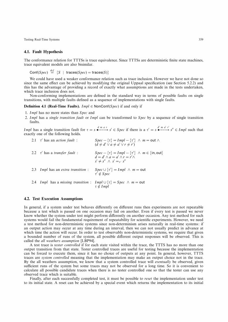
For unit and integration testing we generated exhaustive tests. We can also select test cases from a timeinterval using the traditional domain test technique of selecting boundary values and a middle value. In thetrain-gate specification, the train may approach the crossing at any time between 60 and 120 time units ofanother train leaving the crossing. We now test the system response for just the lower and upper boundsof this time interval, (x==60) and (x==120) and for a middle value (x==90). Figure 3 shows the modifiedprocess Train30. In selecting inputs 30 time steps apart, the tester is assuming that the implementation’sbehaviour between these points is smooth and that no significant behaviours will be ignored. The reductionin TTTS size achieved by using the selective specification can be seen in Table 3: (43,90) for pview comparedwith (83,658) for sview.

Testing Real-Time Systems 365
6. Conclusions
We have presented a conformance test method for real-time systems specified by networks of timed automata.The method introduces test views, a testable model for real-time systems (TTTS) and presents fault hypothesesand a conformance test generation algorithm for TTTSs. We have argued that this method provides a practicalbasis for conformance testing of real-time systems since,
1. Using test views can significantly reduce the size of the full TTTS for a system and, in turn, reduce thenumber of test cases to be executed. Each view makes visible only the events of interest for a particulartest purpose.
2. The conformance test algorithm for TTTSs makes effective use of features such as persistent variables tominimise the number of test cases required.
3. An easily readable record of exactly what has been tested is available. This facilitates communicationbetween the system’s developers, testers and customers. Testers can use independent test methods to checkthat assumptions made are reasonable
4. Test and verification of timed automata is only possible with good tool support. The Essex test toolautomatically constructs TTTSs under different views and generates test suites [Glo00]. The user caneasily experiment with different test views and Uppaal specifications.
5. An open environment is provided for real-time systems development. The Essex test tool accepts specifi-cations in Uppaal syntax linking test generation with simulation and verification. We currently have notool support for executing our generated test suites and are considering the use of existing test drivers,such as the VVT system [PeS97], for this purpose.
Complete test suites are expensive to execute, even using the methods of this paper to reduce that cost.We do not recommend that complete conformance test methods are used everywhere, but they should beused for critical parts of a system. For large systems, our method can be combined with traditional partialtest coverage methods such as domain testing or selecting a percentage of all possible traces as test cases.
So far we have constructed TTTSs by generating the full (digital clock) TTS for a specification and thentransforming it under a given view to a TTTS. It would be better, though, to have transformation rules fortimed automata specifications since such rules could also be applied to systems whose intermediate TTTSmodels are infinite or too large to generate. In general, existing abstraction techniques for untimed, reactivesystems [AHR98, LGS95] are difficult to apply to real-time systems because the time taken by hidden eventsmust be remembered in the timing of all future actions. Finding effective abstraction methods for real-timesystems, perhaps along the lines of [JLS00], is an interesting open problem which will be addressed in ourfuture work.
Acknowledgements
This work was supported by EPSRC grant GR/L26087: Integrating Test and Verification for Real-Time andFault-Tolerant Systems in a Trustworthy Tool. Tim Glover implemented the Essex test generation tool. I amgrateful to the anonymous referees and to Thorsten Gerdsmeier, Norbert Volker, Tim Glover, Sam Steel, andparticipants of the 11th Nordic Workshop on Programming Theory for their insightful comments on thiswork.
References
[AlD94] Alur, R. and Dill, D. L.: A Theory of Timed Automata, Theoretical Computer Science 126, pp. 183–235 (1994)[AFH94] Alur, R., Fix, L. and Henzinger, T.: Event-Clock Automata: A Determinizable Class of Timed Automata, In 6th International
Conference on Computer Aided Verification, LNCS 818, pp. 1–13, Springer Verlag (1994)[AHR98] Alur, R., Henzinger, T. and Rajamani, S.: Symbolic Exploration of Transition Hierarchies, In Tools and Algorithms for the
Construction and Analysis of Systems, LNCS 1384, pp. 330–344, Springer Verlag (1998)[BFM97] Braberman, V., Felder, M. and Marre, M.: Testing Timing Behaviours of Real Time Software, In Quality Week 1997.
San Francisco, USA, pp. 143–155 (1997)[CaG98] Cardell-Oliver, R. and Glover, T.: A Practical and Complete Algorithm for Testing Real-Time Systems, In Formal Techniques
in Real-Time and Fault-Tolerant Systems, LNCS 1486, pp. 251–260, Springer Verlag (1998)

366 R. Cardell-Oliver
[Cho78] Chow, T. S.: Testing Software Design Modeled by Finite-State Machines, In IEEE Transactions on Software EngineeringVol SE-4, No. 3, pp. 178–187 (1978)
[ClL95] Clarke, D. and Lee, I.: Testing Real-Time Constraints in a Process Algebraic Setting, In 17th International Conference onSoftware Engineering, (1995)
[EDK98] En-Nouaary, A., Dssouli, R., Khendek, F. and Elqortobi, A.: Timed Test Cases Generation Based on State CharacterisationTechnique, In 19th IEEE Real-Time Systems Symposium (RTSS’98), pp. 220–229 (1998)
[Glo00] Glover, T.: TestFrame: A Test Generation Tool for Real-Time Systems, Department of Computer Science Technical ReportCSM-336, University of Essex, March (2000)
[HMP92] Henzinger, T., Manna, Z. and Pnueli, A.: What Good are Digital Clocks? In Proc. 19th International Colloquium onAutomata, Languages, and Programming, Lecture Notes in Computer Science 632, Springer-Verlag, pp. 545–558 (1992)
[HNT99] Higashino, T., Natata, A., Taniguchi, K. and Cavalli, A. R.: Generating Test Cases for a Timed I/O Automaton Model, InIFIP TC6 International Workshop on Testing of Communicating Systems (1999)
[Hol91] Holzmann, G. J.: Design and Validation of Computer Protocols, Prentice Hall (1991)[HoU79] Hopcroft, J. and Ullman, J.: Automata Theory, Addison-Wesley (1979)[JLS00] Jensen, H. E., Larsen, K. G. and Skou, A.: Scaling Up Uppaal: Automatic Verification of Real-Time Systems using
Compositionality and Abstraction. To appear in Formal Techniques for Real-Time and Fault-Tolerant Systems, LectureNotes in Computer Science, Springer Verlag (2000)
[LPW97] Larsen, K. G., Pettersson, P. and Wang, Y.: UPPAAL in a Nutshell, In Springer International Journal of Software Tools forTechnology Transfer, 1 (1+2), (1997) source: http://www.docs.uu.se/docs/rtmv/uppaal
[LGS95] Loiseaux, C., Graf, S., Sifakis, J., Bouajjani, A. and Bensalem, S.: Property Preserving Abstractions for the Verification ofConcurrent Systems, Formal Methods in System Design, 6 pp. 1–35 (1995)
[LBP94] Luo, G., Bochmann, G. von and Petrenko, A.: Test Selection Based on Communicating Nondeterministic Finite-StateMachines Using and Generalised WP-Method, IEEE Trans. on Software Engineering, 20 (2), pp. 149–162 (1994)
[MMM95] Mandrioli, D., Morasca, S. and Morzenti, A.: Generating Test Cases for Real-Time Systems from Logic Specifications,ACM Trans. on Computer Systems 13 (4) pp. 365–398 (1995)
[PeS97] Peleska, J. and Siegel, M.: Test Automation of Safety-Critical Reactive Systems, South African Computer Journal 19,pp. 53–77 (1997)
[Pfl98] Pfleeger, S. L.: Software Engineering: Theory and Practice, Prentice Hall (1998)[RaS97] Raskin, J. F. and Schoebbens, P.: Real-Time Logics: Fictitious Clock as an Abstraction of Dense Time, In E. Brinksma (ed.)
Tools and Algorithms for the Construction and Analysis of Systems, Lecture Notes in Computer Science 1217, Springer-Verlag,pp. 165–180 (1997)
[SMH99] Schlingoff, H., Meyer, O. and Hulsing, T.: Correctness Analysis of an Embedded Controller, In Data Systems in Aerospace(DASIA99), ESA SP-447, Lisbon, Portugal, pp. 317–325 (1999)
[SVD99] Springintveld, J., Vaandrager, F. and D’Argenio, P.: Testing Timed Automata, To appear in Theoretical Computer Sciencesource: http://www.cs.kun.nl/~fvaan/publications
[TaP98] Tan, Q. M. and Petrenko, A.: Test generation for specifications modeled by input/output automata, In Proceedings ofthe IFIP TC6 11th International Workshop on Testing of Communicating Systems, Kluwer Academic Publishers, pp. 83–100(1998)
[Tre96] Tretmans, J.: Test Generation with Inputs, Outputs and Quiescence, In T. Margaria and B. Steffen (eds.) Tools and Algorithmsfor the Construction and Analysis of Systems, Lecture Notes in Computer Science 1055, Springer-Verlag pp. 127–146 (1996)
[Upp99] Uppaal: Validation and Verification Tools for Real-Time Systems, http://www.docs.uu.se/docs/rtmv/uppaal, 13October (1999)
[Yov95] Yovine, S.: Model Checking Timed Automata, In G. Rozenberg and F. Vaandrager (eds.), Lectures on Embedded Systems,Lecture Notes in Computer Science 1494, pp. 114–152, Springer Verlag (1996)
Appendix
Worked Example of TTTS Derivation and Test Generation
A very simple timed automata specification is used with two processes: an environment offering a ready syn-chronisation whenever the system is able to accept it, and a system which first accepts a ready synchronisationand creates a 0,1 (on,off) state, then within 3 time units moves to a 1,1 state and within a further 2 timeunits returns to the original 0,0 state and performs the next ready synchronisation. The following TTTSs weregenerated by the Essex test tool.
------------------------------------------------------------------// Very Simple Uppaal TA Specification// ---------------------------------------// 31-viii-00 RCO// ---------------------------------------
clock x, y;urgent chan ready;int off,on;
Testing Real-Time Systems 367
process Environ{state e0{x<=5};init e0;trans e0 -> e0 {sync ready?; assign x:=0; };}process Sys{state s0, s1{y<=3}, s2{y<=2};init s0;trans s0 -> s1 {sync ready!; assign off:=1,y:=0; },s1 -> s2 {guard y<=3; assign on:=1,y:=0; },s2 -> s0 {guard y<=2; assign on:=0,off:=0,y:=0; };}
system Environ, Sys;------------------------------------------------------------------
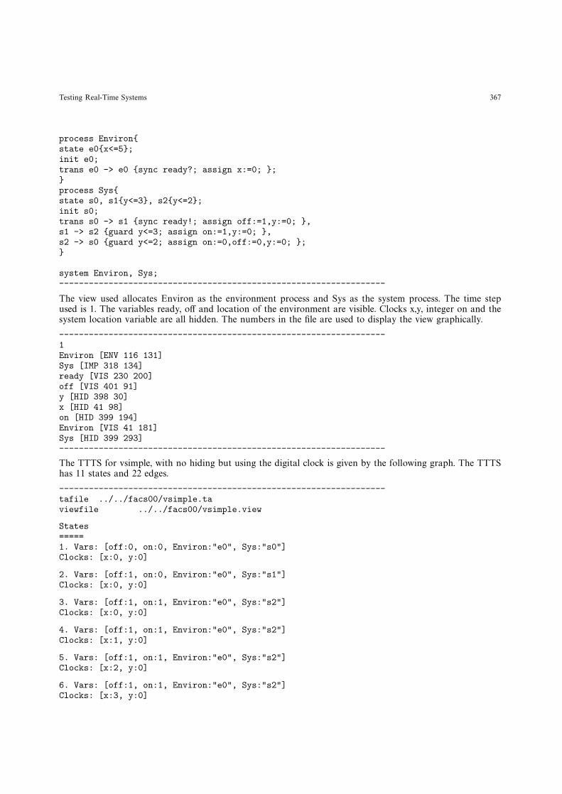
The view used allocates Environ as the environment process and Sys as the system process. The time stepused is 1. The variables ready, off and location of the environment are visible. Clocks x,y, integer on and thesystem location variable are all hidden. The numbers in the file are used to display the view graphically.
------------------------------------------------------------------1Environ [ENV 116 131]Sys [IMP 318 134]ready [VIS 230 200]off [VIS 401 91]y [HID 398 30]x [HID 41 98]on [HID 399 194]Environ [VIS 41 181]Sys [HID 399 293]------------------------------------------------------------------
The TTTS for vsimple, with no hiding but using the digital clock is given by the following graph. The TTTShas 11 states and 22 edges.
------------------------------------------------------------------tafile ../../facs00/vsimple.taviewfile ../../facs00/vsimple.view
States=====1. Vars: [off:0, on:0, Environ:"e0", Sys:"s0"]Clocks: [x:0, y:0]
2. Vars: [off:1, on:0, Environ:"e0", Sys:"s1"]Clocks: [x:0, y:0]
3. Vars: [off:1, on:1, Environ:"e0", Sys:"s2"]Clocks: [x:0, y:0]
4. Vars: [off:1, on:1, Environ:"e0", Sys:"s2"]Clocks: [x:1, y:0]
5. Vars: [off:1, on:1, Environ:"e0", Sys:"s2"]Clocks: [x:2, y:0]
6. Vars: [off:1, on:1, Environ:"e0", Sys:"s2"]Clocks: [x:3, y:0]

368 R. Cardell-Oliver
7. Vars: [off:0, on:0, Environ:"e0", Sys:"s0"]Clocks: [x:1, y:0]
8. Vars: [off:0, on:0, Environ:"e0", Sys:"s0"]Clocks: [x:2, y:0]
9. Vars: [off:0, on:0, Environ:"e0", Sys:"s0"]Clocks: [x:3, y:0]
10. Vars: [off:0, on:0, Environ:"e0", Sys:"s0"]Clocks: [x:4, y:0]
11. Vars: [off:0, on:0, Environ:"e0", Sys:"s0"]Clocks: [x:5, y:0]
Edges=====1->2[Sys(0) (0) [x:=0, Environ:="e0", y:=0, off:=1, Sys:="s1", ready:="sync"]]2->3[Sys(0) (0) [y:=0, on:=1, Sys:="s2"]]2->4[Sys(0) (1) [y:=0, on:=1, Sys:="s2"]]2->5[Sys(0) (2) [y:=0, on:=1, Sys:="s2"]]2->6[Sys(0) (3) [y:=0, on:=1, Sys:="s2"]]3->1[Sys(0) (0) [y:=0, off:=0, on:=0, Sys:="s0"]]3->7[Sys(0) (1) [y:=0, off:=0, on:=0, Sys:="s0"]]3->8[Sys(0) (2) [y:=0, off:=0, on:=0, Sys:="s0"]]4->7[Sys(0) (0) [y:=0, off:=0, on:=0, Sys:="s0"]]4->8[Sys(0) (1) [y:=0, off:=0, on:=0, Sys:="s0"]]4->9[Sys(0) (2) [y:=0, off:=0, on:=0, Sys:="s0"]]5->8[Sys(0) (0) [y:=0, off:=0, on:=0, Sys:="s0"]]5->9[Sys(0) (1) [y:=0, off:=0, on:=0, Sys:="s0"]]5->10[Sys(0) (2) [y:=0, off:=0, on:=0, Sys:="s0"]]6->9[Sys(0) (0) [y:=0, off:=0, on:=0, Sys:="s0"]]6->10[Sys(0) (1) [y:=0, off:=0, on:=0, Sys:="s0"]]6->11[Sys(0) (2) [y:=0, off:=0, on:=0, Sys:="s0"]]7->2[Sys(0) (0) [x:=0, Environ:="e0", y:=0, off:=1, Sys:="s1", ready:="sync"]]8->2[Sys(0) (0) [x:=0, Environ:="e0", y:=0, off:=1, Sys:="s1", ready:="sync"]]9->2[Sys(0) (0) [x:=0, Environ:="e0", y:=0, off:=1, Sys:="s1", ready:="sync"]]10->2[Sys(0) (0) [x:=0, Environ:="e0", y:=0, off:=1, Sys:="s1", ready:="sync"]]11->2[Sys(0) (0) [x:=0, Environ:="e0", y:=0, off:=1, Sys:="s1", ready:="sync"]]------------------------------------------------------------------
After hiding and eliding any invisible edges we have the following TTTS with 7 states and 18 edges.
------------------------------------------------------------------tafile ../../facs00/vsimple.taviewfile ../../facs00/vsimple.view
States=====1. Vars: [off:0, on:0, Environ:"e0", Sys:"s0"]Clocks: [x:0, y:0]
2. Vars: [off:1, on:0, Environ:"e0", Sys:"s1"]Clocks: [x:0, y:0]
3. Vars: [off:0, on:0, Environ:"e0", Sys:"s0"]Clocks: [x:1, y:0]
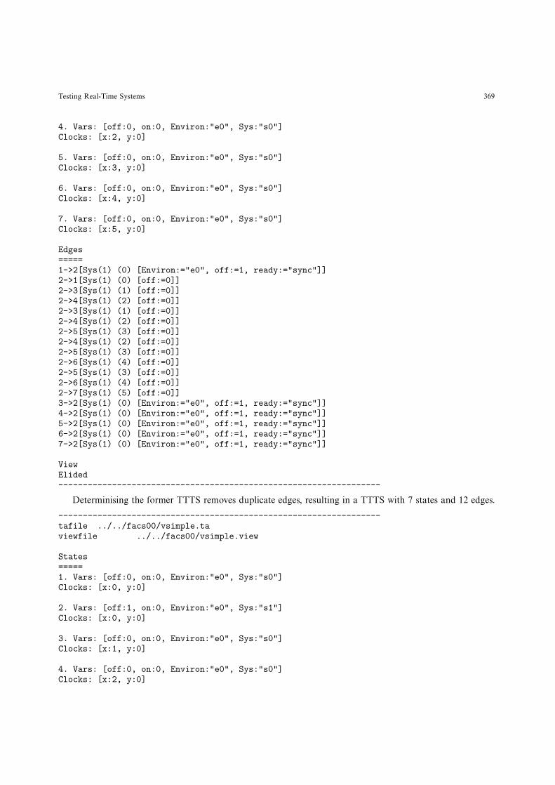
Testing Real-Time Systems 369
4. Vars: [off:0, on:0, Environ:"e0", Sys:"s0"]Clocks: [x:2, y:0]
5. Vars: [off:0, on:0, Environ:"e0", Sys:"s0"]Clocks: [x:3, y:0]
6. Vars: [off:0, on:0, Environ:"e0", Sys:"s0"]Clocks: [x:4, y:0]
7. Vars: [off:0, on:0, Environ:"e0", Sys:"s0"]Clocks: [x:5, y:0]
Edges=====1->2[Sys(1) (0) [Environ:="e0", off:=1, ready:="sync"]]2->1[Sys(1) (0) [off:=0]]2->3[Sys(1) (1) [off:=0]]2->4[Sys(1) (2) [off:=0]]2->3[Sys(1) (1) [off:=0]]2->4[Sys(1) (2) [off:=0]]2->5[Sys(1) (3) [off:=0]]2->4[Sys(1) (2) [off:=0]]2->5[Sys(1) (3) [off:=0]]2->6[Sys(1) (4) [off:=0]]2->5[Sys(1) (3) [off:=0]]2->6[Sys(1) (4) [off:=0]]2->7[Sys(1) (5) [off:=0]]3->2[Sys(1) (0) [Environ:="e0", off:=1, ready:="sync"]]4->2[Sys(1) (0) [Environ:="e0", off:=1, ready:="sync"]]5->2[Sys(1) (0) [Environ:="e0", off:=1, ready:="sync"]]6->2[Sys(1) (0) [Environ:="e0", off:=1, ready:="sync"]]7->2[Sys(1) (0) [Environ:="e0", off:=1, ready:="sync"]]
ViewElided------------------------------------------------------------------
Determinising the former TTTS removes duplicate edges, resulting in a TTTS with 7 states and 12 edges.
------------------------------------------------------------------tafile ../../facs00/vsimple.taviewfile ../../facs00/vsimple.view
States=====1. Vars: [off:0, on:0, Environ:"e0", Sys:"s0"]Clocks: [x:0, y:0]
2. Vars: [off:1, on:0, Environ:"e0", Sys:"s1"]Clocks: [x:0, y:0]
3. Vars: [off:0, on:0, Environ:"e0", Sys:"s0"]Clocks: [x:1, y:0]
4. Vars: [off:0, on:0, Environ:"e0", Sys:"s0"]Clocks: [x:2, y:0]

370 R. Cardell-Oliver
5. Vars: [off:0, on:0, Environ:"e0", Sys:"s0"]Clocks: [x:3, y:0]
6. Vars: [off:0, on:0, Environ:"e0", Sys:"s0"]Clocks: [x:4, y:0]
7. Vars: [off:0, on:0, Environ:"e0", Sys:"s0"]Clocks: [x:5, y:0]
Edges=====1->2[Sys(1) (0) [Environ:="e0", off:=1, ready:="sync"]]2->1[Sys(1) (0) [off:=0]]2->3[Sys(1) (1) [off:=0]]2->4[Sys(1) (2) [off:=0]]2->5[Sys(1) (3) [off:=0]]2->6[Sys(1) (4) [off:=0]]2->7[Sys(1) (5) [off:=0]]3->2[Sys(1) (0) [Environ:="e0", off:=1, ready:="sync"]]4->2[Sys(1) (0) [Environ:="e0", off:=1, ready:="sync"]]5->2[Sys(1) (0) [Environ:="e0", off:=1, ready:="sync"]]6->2[Sys(1) (0) [Environ:="e0", off:=1, ready:="sync"]]7->2[Sys(1) (0) [Environ:="e0", off:=1, ready:="sync"]]
ViewElidedDeterminised------------------------------------------------------------------
The final normalisation step is to minimise the preceding TTTS. Note that since the environment’s clockx is hidden, the states 3,4,5,6 and 7 are all visibly equivalent, and they have the same set of possible traces.Therefore, 4 of these 5 states are redundant, and after minimisation we have a TTTS of 2 states and 7 edges.Both the remaining states are visibly distinguishable and so no distinguishing sequences are required. If x hadbeen left visible, then states 3 to 7 would have been visibly distinguishable and the final test TTTS wouldhave remained with 7 states and 12 edges.
------------------------------------------------------------------tafile ../../facs00/vsimple.taviewfile ../../facs00/vsimple.view
States=====1. Vars: [off:0, on:0, Environ:"e0", Sys:"s0"]Clocks: [x:0, y:0]
2. Vars: [off:1, on:0, Environ:"e0", Sys:"s1"]Clocks: [x:0, y:0]
Edges=====1->2[Sys(1) (0) [Environ:="e0", off:=1, ready:="sync"]]2->1[Sys(1) (0) [off:=0]]2->1[Sys(1) (1) [off:=0]]2->1[Sys(1) (2) [off:=0]]2->1[Sys(1) (3) [off:=0]]2->1[Sys(1) (4) [off:=0]]2->1[Sys(1) (5) [off:=0]]

Testing Real-Time Systems 371
ViewElidedDeterminisedMinimised------------------------------------------------------------------
Next generate test sequences from this TTTS.
------------------------------------------------------------------reach(1) = { <> }reach(2) = { <0/ready/off:=1> }
distinguish 1 from 2 = { <>*yes }distinguish 2 from 1 = { <>*yes}
testsfor(1) = { <>*yes }testsfor(2) = {<0/ready/off:=1, 0/off:=0>*yes,<0/ready/off:=1, 1/off:=0>*yes,<0/ready/off:=1, 2/off:=0>*yes,<0/ready/off:=1, 3/off:=0>*yes,<0/ready/off:=1, 4/off:=0>*yes,<0/ready/off:=1, 5/off:=0>*yes }
Tests vsimple = {<0/ready/off:=1, 0/off:=0>*yes,<0/ready/off:=1, 1/off:=0>*yes,<0/ready/off:=1, 2/off:=0>*yes,<0/ready/off:=1, 3/off:=0>*yes,<0/ready/off:=1, 4/off:=0>*yes,<0/ready/off:=1, 5/off:=0>*yes }------------------------------------------------------------------
Received October 1999
Accepted in revised form November 2000 by C. B. Jones