configural frequency analysis in applied psychological research

APPLIED PSYCHOLOGY: AN INTERNATIONAL REVIEW, 19%, 45 (4). 301-352

Lead Article

Configural Frequency Analysis in Applied Psychological Research

Alexander von Eye Michigan State University, USA

Christiane Spiel University of Vienna, Austria

Phillip K. Wood University of Missouri, Columbia, USA

L’Analyse de Frtquence des Configurations (AFC) est une mtthode de recherche des classes et anticlasses dans les classifications croiskes de catkgories de variables. Les classes sont des modtles de cattgories de variables qui apparaissent plus souvent que le hasard ne le laisse supposes. Les anticlasses sont des modtles de catkgorie de variables qui apparaissent moins souvent que le hasard ne le laisse supposes. On prksente quatre applications d’AFC: I’AFC de premier ordre, I’AFC prtdictive, I’AFC de symttrie axiale, et un modtle d’AFC longitudinale. On examine les caracttristiques de I’AFC en insistant sur les contraintes et I’applicabilitt. On compare aussi I’AFC avec d’autres mkthodes permettant l’analyse multivarite de catkgories de donntes, en particulier la modtlisation log-linkaire. Des sorties informatiques sont traittes.

Configural Frequency Analysis (CFA) is a method for the search for types and antitypes in cross-classifications of categorical variables. Types are patterns of variable categories that occur more often than expected from chance. Antitypes are patterns of variable categories that occur less often than expected from chance. Four applications of CFA are reviewed: the First Order CFA, the Prediction CFA, Axial Symmetry CFA, and one model of

Requests for reprints should be sent to Alexander von Eye, Michigan State University,

Parts of Alexander von Eye’s work on this paper were supported by a grant from the Mary Department of Psychology, 119 Snyder Hall, East Lansing, MI 488241117, USA.

Louis Foundation.

0 1996 International Association of Applied Psychology

302 VON EYE, SPIEL, WOOD

Longitudinal CFA. Characteristics of CFA are discussed, focusing on constraints posed and applicability. Comparisons are made of CFA with other methods for multivariate analysis of categorical data, in particular, log-linear modelling. Computational issues are discussed.

INTRODUCTION This paper discusses Configural Frequency Analysis (CFA) as a statistical method for the search for types and antitypes of categorical data in applied psychological research. The first section describes the method of CFA. The following sections present sample models of CFA as well as sample applications.

1. CONFIGURAL FREQUENCY ANALYSIS: THE SEARCH FOR TYPES AND ANTITYPES

In applied psychological research as well as in other academic endeavours one often asks questions concerning “most typical” and “most atypical” behaviour patterns in described populations. For example, one often encounters questions concerning typical behaviours in which city dwellers differ from people living in rural environments. Similarly, in psychopathology one finds statements describing behaviours that are most typical of neurotics, schizophrenics, or depressed patients. In personality, researchers describe behaviour patterns typical of extroverts; in school psychology one asks for patterns of learning behaviour that seem most promising. In industrial psychology one asks what cars are typically considered by female buyers. In leisure studies one asks what are the typical characteristics of adolescents that do participate in certain kinds of extracurricular activities and what are the typical characteristics of adolescents that do not participate.

CFA (Lienert, 1969, 1988; von Eye, 1990) is a statistical method that allows one to answer questions concerning typical or atypical behaviours. Specifically, CFA allows one to identify variable patterns that are, relative to some expectation, more frequent (typical) or less frequent (atypical). This paper presents CFA as a sample case of a versatile, multivariate, non- parametric and robust statistical method that is useful without requiring extensive computing. The following sections present a brief tutorial of CFA. Four CFA models are introduced: the classic First Order CFA, the Prediction CFA, Axial Symmetry CFA, and Longitudinal CFA. Subsequent sections present applications of these models using empirical data, and discuss CFA in comparison with other multivariate statistical methods, specifically log-linear modelling.

APPLIED CFA 303

1.1 introduction to Configural Frequency Analysis: A Tutorial

This section introduces readers to main concepts of CFA. Data examples follow in Section 2. CFA is a statistical method for multivariate analysis of categorical variables. In multivariate research, two or more categorical variables are of interest. The most important advantage of multivariate research is that variables' joint distributional characteristics can be analysed above and beyond their univariate characteristics. These multivariate characteristics can be approached from two perspectives. The first focuses on variables. Statements resulting from this perspective concern variables' joint frequency distributions, interactions (association patterns), and dependency relationships (Goodman, 1981). Log-linear models are most typically used to specify such statements.

The second perspective focuses on cases: that is, subjects or respondents. In other contexts, this perspective is termed person-approach to cross- classifications' (Bergman, Eklund, & Magnusson, 1991). One question often asked from this perspective is whether variable characteristics can be identified that differ in frequency from what was expected from some chance model (this term is explained later). For instance, one can ask whether young male drivers are involved in car accidents more often than one would expect from chance alone: that is, without consideration of gender and age. In other contexts one may ask whether psychiatric syndromes, i.e. symptom patterns, occur more often in older people than in younger people. CFA is a method that focuses on cases.

The following sections introduce readers to technical aspects of CFA. Chance models are presented as well as statistical methods for answering questions of the type posed earlier.

7 . 7 . 1 CFA: Goals of Analysis and Chance Models

When crossing more than two variables, one creates contingency tables (also termed tabular arrays or cross-classifications) the cells of which can be labelled using variable indexes. In CFA terminology, patterns of variable indexes are called configurations. It is the goal of CFA to determine for each configuration whether it constitutes a type or an antitype. Types and antitypes are identified by comparing observed with expected cell frequencies in individual cells of a cross-classification.

'Contrasting the variables approach with the person approach presupposes that frequencies describe behaviour of humans. In a more general sense, the person approach can also be termed the differentialapproach. I t is the goal of the differential approach to identify subgroups of cases that are unique in displaying characteristics at rates not predicted by chance (cf Emmerich, 1968).


Let e be an expected cell frequency, estimated under some chance model, and o the observed cell frequency. CFA asks for each cell whether, statistically,

o + e . (1) If o > e, the configuration for which this occurred is termed a type. If, in contrast, o < e, the configuration is termed an antitype.

To determine the expected cell frequency, e, one uses chance models. Such models, also termed null models, of CFA construct a theoretical rendering of the population under study that has the following two characteristics (cf von Eye & Sthensen, 1991; Wickens, 1989):

1. It considers all relationships among variables, with only one exception,

2. relationships that define the model under study are assumed not to that is:

exist.

There is only one way to contradict this type of a chance model: the variable relationships assumed not to exist, do exist. The following example illustrates the concept of a chance model. Consider the variables intelligence, work habits, and marks in school. Some researcher assumes that, across all levels of intelligence, work habits predict performance in school. A chance model would then assume that intelligence and work habits are related to each other, and that intelligence and marks are related to each other (Characteristic 1 of chance models), and that work habits and marks are unrelated (Characteristic 2 of chance models). This model can be contradicted only if either work habits and marks are related to each other or if there is a triple interaction between intelligence, work habits, and marks.

In CFA, chance models can be classified into two major groups (von Eye, 1990):

1. Global CFA Models. In these models all variables have the same status in the sense that there are no such groups of variables as predictors and criteria (for examples see below).

Within the group of global CFA models there is a hierarchy of models. Hierarchy levels are determined by the order of relationships assumed. For instance, zero order models assume neither variable relationships nor variable main effects. Any deviation from equal probability contradicts this chance model. Accordingly, the First Order CFA model, which is the classical CFA model (Lienert, 1969), assumes that no variable relationships of any kind exist. Variable main effects, however, may exist. This chance model can be contradicted only if there are variable relationships. The

APPLIED CFA 305

higher the hierarchical level, the fewer “chances” there are to contradict the model. The first order CFA model is also termed the model ofroral variable independence or classic CFA model.

2 . Regional CFA Models. In these models, variables are grouped. For instance, there can be the groups of predictors and criteria, of dependent and independent variables. Or, there can be groupings based on substantive considerations, for example, the group of motivation-related variables and the group of performance-related variables.

Regional CFA chance models make two assumptions. The first assumption allows for any type of relationship among variables in the same group. The second assumption is that variable groups are independent of each other. This set of assumptions can be contradicted only if there are relationships between variables from different groups.

1.1.2 Log-linear Models for Estimation of Expected Cell Frequencies

As was shown by von Eye (1988,1990), most CFA chance models can be cast in terms of log-linear models. Important from a computational perspective is that most CFA models belong to the class of simple log-linear models (Goodman, 1978) which share the characteristic that their expected cell frequencies can be estimated directly from the marginals. In other words, expected cell frequencies for simple log-linear models can be estimated by inserting marginals into formulas only once rather than going through possibly lengthy iterations. The number of steps involved when performing CFA can be precisely determined. Many CFA models require only minimal computational effort.

In this section, we present log-linear models that represent CFA chance models, and formulas for estimating expected cell frequencies for three CFA models. The first is the global and classical, First Order CFA model. The second is the regional model of Prediction CFA (P-CFA). The third is the Model of Axial Symmetry, and the fourth is a model for Longitudinal CFA. Data examples follow in Section 2.

However, before specifying models and giving formulas for estimation of expected cell frequencies, we discuss the role played by log-linear models for CFA. For CFA applications the values of the model parameters are not of interest, and neither are their numerical values or the overall model fit. The model only plays one role. It is a vehicle to translate a CFA model into a form that allows one to estimate expected cell frequencies. Accordingly,


specification of a log-linear model that describes the data well is not the goal of CFA. Rather, CFA searches for those cells that contain so many or so few cases that they statistically contradict the log-linear model: that is, the chance model. Interpretation of CFA results focuses on characteristics of these cases.

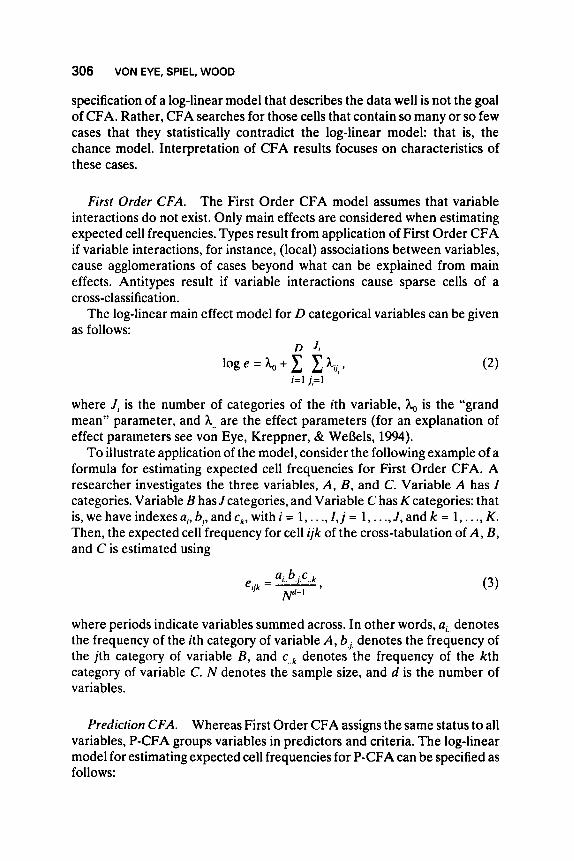
First Order CFA. The First Order CFA model assumes that variable interactions do not exist. Only main effects are considered when estimating expected cell frequencies. Types result from application of First Order CFA if variable interactions, for instance, (local) associations between variables, cause agglomerations of cases beyond what can be explained from main effects. Antitypes result if variable interactions cause sparse cells of a cross-classification.

The log-linear main effect model for D categorical variables can be given as follows:

D log e = h, + C A;,, ,

i=l j,=1

where J , is the number of categories of the ith variable, h, is the “grand mean” parameter, and A.. are the effect parameters (for an explanation of effect parameters see von Eye, Kreppner, & WeBels, 1994).

To illustrate application of the model, consider the following example of a formula for estimating expected cell frequencies for First Order CFA. A researcher investigates the three variables, A, B, and C. Variable A has I categories. Variable B hasJ categories, and Variable C has K categories: that is, we have indexes a,, b,, and ck, with i = 1, . . ., I, j = 1,. . ., J, and k = 1,. . ., K. Then, the expected cell frequency for cell ijk of the cross-tabulation of A, B, and C is estimated using

where periods indicate variables summed across. In other words, ui,, denotes the frequency of the ith category of variable A, 6,j, denotes the frequency of the j th category of variable B, and c , , ~ denotes the frequency of the kth category of variable C. N denotes the sample size, and d is the number of variables.

Prediction CFA. Whereas First Order CFA assigns the same status to all variables, P-CFA groups variables in predictors and criteria. The log-linear model for estimating expected cell frequencies for P-CFA can be specified as follows:

APPLIED CFA 307

1. It is saturated in the predictors, i.e. any possible relationship between predictors may exist;

2. it is saturated in the criteria; 3. there is independence between predictors and criteria.

The P-CFA model can be violated only if there are relationships between predictors and criteria. These relationships manifest in form of types and antitypes.

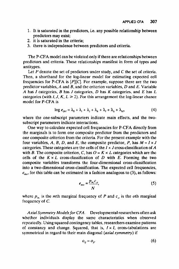
Let P denote the set of predictors under study, and C the set of criteria. Then, a shorthand for the log-linear model for estimating expected cell frequencies for P-CFA is [ P ] [ C ] . For example, suppose there are the two predictor variables, A and B, and the criterion variables, D and E. Variable A has I categories, B has J categories, D has K categories, and E has L categories (with I, J , K, L 3 2). For this arrangement the log-linear chance model for P-CFA is

log eijkl = A,, + hi + h, + h, + h, + hi, + h,,, (4)

where the one-subscript parameters indicate main effects, and the two- subscript parameters indicate interactions.

One way to calculate expected cell frequencies for P-CFA directly from the marginals is to form one composite predictor from the predictors and one composite criterion from the criteria. For the present example with the four variables, A, B, D, and E, the composite predictor, P, has M = I x J categories. These categories are the cells of the I x J cross-classification of A with B. The composite criterion, C, has 0 = K x L categories which are the cells of the K x L cross-classification of D with E. Forming the two composite variables transforms the four-dimensional cross-classification into a two-dimensional cross-classification. The expected cell frequencies, emu. for this table can be estimated in a fashion analogous to (3), as follows:

where p,, is the mth marginal frequency of P and c , ~ is the 0th marginal frequency of C.

Axial Symmetry Models for CFA. Developmental researchers often ask whether individuals display the same characteristics when observed repeatedly. Using squared contingency tables, researchers examine patterns of constancy and change. Squared, that is, I x I, cross-tabulations are symmetrical in regard to their main diagonal (axial symmetry) if

(6 ) 0.. = o... IJ 11


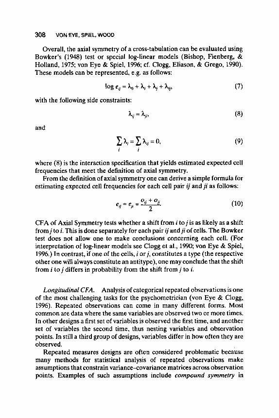
Overall, the axial symmetry of a cross-tabulation can be evaluated using Bowker’s (1948) test or special log-linear models (Bishop, Fienberg, & Holland, 1975; von Eye & Spiel, 1996; cf. Clogg, Eliason, & Grego, 1990). These models can be represented, e.g. as follows:

log ejj = h, + hi + hi + h,, (7)

with the following side constraints:

hij = A,, (8)

and

h; = c hjj = 0, i i

(9)

where (8) is the interaction specification that yields estimated expected cell frequencies that meet the definition of axial symmetry.

From the definition of axial symmetry one can derive a simple formula for estimating expected cell frequencies for each cell pair ij and ji as follows:

oij + oj; e.. = e.. = -. ‘I I‘ 2

CFA of Axial Symmetry tests whether a shift from i to j is as likely as a shift from j to i. This is done separately for each pair ij and ji of cells. The Bowker test does not allow one to make conclusions concerning each cell. (For interpretation of log-linear models see Clogg et al., 1990, von Eye & Spiel, 1996.) In contrast, if one of the cells, i or j , constitutes a type (the respective other one will always constitute an antitype), one may conclude that the shift from i to j differs in probability from the shift from j to i.

Longitudinal CFA. Analysis of categorical repeated observations is one of the most challenging tasks for the psychometrician (von Eye & Clogg, 1996). Repeated observations can come in many different forms. Most common are data where the same variables are observed two or more times. In other designs a first set of variables is observed the first time, and another set of variables the second time, thus nesting variables and observation points. In still a third group of designs, variables differ in how often they are observed.

Repeated measures designs are often considered problematic because many methods for statistical analysis of repeated observations make assumptions that constrain variancexovariance matrices across observation points. Examples of such assumptions include compound symmetry in

APPLIED CFA 309

ANOVA which assumes equal variances and covariances across observation points. CFA does not make such assumptions. In contrast, it focuses on the dependence structure. It asks whether there exist types and antitypes that reflect the time-related dependence structure. Thus, the existence of time-related dependence structures is not a reason for distrusting CFA results. Rather, CFA identifies and describes such structures.

Although very robust in the sense that data of a wide range of characteristics can be analysed using CFA, longitudinal CFA nevertheless must entail assumptions concerning data characteristics in order to be tractable. One of the most important assumptions is that each individual provides the same number of data points. In designs where the number of variables is the same for each respondent, and where the number of responses was determined before data collection, participants typically provide the same number of data points. However, when studying such behaviours as dialogues where the number of times a dialogue partner talks is not a priori determined, the amount of data provided by respondents can vary widely. Until recently, this topic had only been recognised (Wickens, 1989) but there were no solutions. There are approaches to solving the problem using weighting procedures (Hecker & Wiese, 1994). However, the usefulness of this type of method for CFA still has to be investigated.

For this reason, the following presentation of longitudinal CFA focuses on designs where the same variables are repeatedly observed, and each participant provides the same number of responses. Consider the case where one variable, X, is observed T = 4 times ( r = 1, . . ., 4). The log-linear chance model for longitudinal CFA of these data is

T

where i, j , k, and 1 index the categories of the observed variable, X, at the observation points. The closed-form equation for estimation of expected cell frequencies for this model of longitudinal CFA can be formulated in a fashion analogous to (3). (For additional models of longitudinal CFA see von Eye, 1990.)

The model of longitudinal CFA given in (11) assumes that the values observed for the repeatedly observed variable, X, are totally independent of each other over time. Types and antitypes will exist only if there are time-related autocorrelations of first or higher order.

The model given in (11) can be altered to accommodate additional variables, for example, covariates, and various assumptions concerning the autocorrelation structure. If autocorrelations are considered, types and antitypes will emerge only if there are variable interactions beyond those assumed in the CFA model.


1.2 Statistical Testing in CFA The typical use of CFA is exploratory. It asks for each cell or, in symmetry testing, for each pair ij/ji of cells, whether the estimated expected cell frequency is statistically different from the observed cell frequency (see Formula 1). Confirmatory use of CFA targets a subset of cells only. This paper focuses on exploratory CFA.

There have been a number of tests proposed for use in CFA (see von Eye, 1990, von Eye & Rovine, 1988; Wood, Sher, & von Eye, 1994). These tests belong to two groups. The first group contains asymptotic tests. They all approximate the binomial test using its relations to such sampling distributions as the normal and the chi-squared distribution. The second group contains tests that assume that marginals are fixed. This group includes, for example, Lehmacher’s (1981) hypergeometric test. Lehmacher’s test and the binomial test are exact tests in the sense that they calculate exact probabilities rather than using approximations to sampling distributions.

The best-known and most widely used asymptotic test in CFA is the Pearson X2 test. The test statistic is a Xz-component which, for df= 1, is asymptotically distributed as x2. For the cross-tabulation of the three variables, A, B, and C, this test statistic is as follows:

A standard normal approximation of the binomial test that can be applied when Npijk 5 10, with pijk = eij/iV. The approximation is defined as follows:

where q = 1 - p . The following relationship holds for df= 1: z2(a/2) = xz(a). When used for CFA-tests, the test statistic given in (13) has two major

advantages over the one given in (12) (see von Eye, 1990). First, it should be noticed that the square root of (12) is not identical to (13). Because q is less than 1, the relationship z > X will always hold and, thus, (13) is a more powerful test than (12). As a result, (13) will allow one to detect more types and antitypes than (12). Second, (13) is symmetrical in the sense that, for a given absolute difference between o and e, the size of the test statistic does not vary with the sign of the difference between o and e. As a result, (13) will allow one to detect clearly more antitypes than (12).

Other test statistics proposed for use in CFA include the F-test (Heilmann & Schiitt, 1985), and the asymptotic version of Lehmacher’s (1981) hypergeometric test. Lehmacher’s (1981) test is often considered because of its superior power. However, when sample sizes are small,

APPLIED CFA 31 1

Lehmacher’s test tends to suggest non-conservative decisions (for a continuity correction see Klichenhoff, 1986). Tests (12) and (13) are often preferred because they are applicable to all CFA models. In contrast, Lehmacher’s (1981) test can be applied only to first order CFA.

1.3 Simultaneous Testing in CFA One of the quasi-irrational traditions in applied statistics is that null hypotheses can be rejected when chances in their favour are less than 5% or less than 1%. In CFA testing and, in general, when more than one test is performed on the same data set, it seems hard to guarantee that this sign8cance level is constant. There are two major reasons for this problem.

The first is known as the problem of mutual dependence of multiple tests. Suppose a researcher applies just one test to a data set. Then, the probability of an a-error is, as was specified, P = 0.05 (always assuming the statistical test was properly applied). When more than one test is applied, one cannot guarantee that these tests are not dependent on each other. For instance, it was shown (Steiger, Shapiro, & Browne, 1985) that X2-tests, when sequentially applied to the same sample, have an asymptotical intercorrelation that can be high. As a result, one can have an actual a much higher than the a priori specified one and erroneously reject true null hypotheses.

Closely interrelated with the problem of mutual dependence of multiple tests is the problem of multiple testing. Suppose a researcher performs a series of statistical tests on the same sample. For each of these tests the researcher admits error rate a. Then, even when these tests are fully independent, after a number of tests the chances are great that the researcher capitalises on chance. In other words, the researcher must assume that some of the “significant” results turned out significant only because of admitting an error rate of a. Consider the following example. A researcher performs 27 CFA tests, each at a = 0.05. Then, the chance of committing three a-errors-that is, making more than 10% wrong decisions-is P = 0.1505, and this is the case even if the tests are fully independent of each other!

Mainly for these two reasons CFA is always performed with a protection. There are three strategies for a protection. The first protects the local level a . It guarantees that a is the error rate for each single test. The second strategy protects the global level a. It guarantees that the probability of at least one false rejection is not greater than a. The third strategy protects the multiple level a. It guarantees that committing the a-error at least once is not greater than a , and this is the case regardless of what other hypotheses must be rejected. In exploratory CFA one typically protects the local level a (Perli, Hommel, & Lehmacher, 1985).

312 VON EVE, SPIEL, WOOD

There have been numerous strategies proposed for a protection (for an overview see von Eye, 1990). Of these, the computionally least burdensome are presented here, the Bonferroni and the Holm (1979) methods for a adjustment.

Suppose a researcher performs r simultaneous tests. The a-error for the ith of these tests is a,, with i = 1,. . ., r. Let a * denote the probability that at least one of the r tests mistakenly suggests that the null hypothesis be rejected. Then, to control the local level a, one must specify a * such that the sum of all a, does not exceed a. In more technical terms, we specify that

1 a, s a. i

For the Bonferroni-adjusted a * one requires in addition, that

a = a*, for all i = 1, . . ., r, (15)

or, in words, that the error rate a be the same for each test. Then the Bonferroni-adjusted a is given by

a r

a * = -.

For the following example suppose a CFA is conducted on a matrix with 36 cells. Then, the typical number of CFA tests is r = 36, and a* = 0.05/36 = 0.001389.

Although Krauth and Lienert’s (1973) results suggest that testing at the Bonferroni-adjusted a is only slightly more conservative, when all r tests are independent of each other, there have been various attempts at devising less conservative test strategies. One well-known approach has been presented by Holm (1979). Holm suggested considering the number of tests already performed when performing the ith test. As a result, the adjusted level a * can no longer be constant. Rather, the Holm-adjusted a for the ith test is defined as

Obviously, for i = 1, that is, for the first test, Holm’s adjusted a* is identical to the constant Bonferroni adjusted a*. However, beginning with the second test, Holm’s a* is less restrictive. Indeed, we find that, for the last test, a* = a. It should be noted that Holm’s (1979) strategy presupposes that test statistics are rank ordered before testing in descending order. Testing terminates as soon as the first difference o - e is not statistically significant.

APPLIED CFA 313

2. DATA EXAMPLES

This section presents data examples for each of the four CFA models discussed in this paper. We assume data are available in tabular form.

2.1 First Order CFA

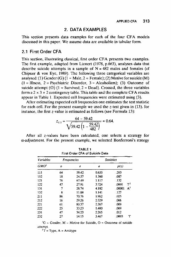
This section, illustrating classical, first order CFA presents two examples. The first example, adapted from Lienert (1978, p.663), analyses data that describe suicide attempts in a sample of N = 482 males and females (cf Chipuer & von Eye, 1989). The following three categorical variables are analysed: (1) Gender (G) (1 = Male, 2 = Female); (2) Motive for suicide (M) (1 = Illness, 2 = Psychiatric Disorder, 3 = Alcoholism); (3) Outcome of suicide attempt (0) (1 = Survived, 2 = Dead). Crossed, the three variables form a 2 x 3 x 2 contingency table. This table and the complete CFA results appear in Table 1. Expected cell frequencies were estimated using (3).

After estimating expected cell frequencies one estimates the test statistic for each cell. For the present example we used the z-test given in (13). for instance, the first z-value is estimated as follows (see Formula 13):

64 - 59.42 = o.64.

After all z-values have been calculated, one selects a strategy for a-adjustment. For the present example, we selected Bonferroni's stategy

TABLE 1 First Order CFA of Suicide Data

~ _ _ _ _ _ _ _ ~ _ _ _ _ _ ~ ~ _ _ _ _ _

Variables Frequencies ~~

Statistics

GMO' 0 e 0 P(Z)

1 1 1 64 59.42 0.635 ,263 112 18 24.57 1.360 .087 121 76 67.49 1.117 .132 122 47 27.91 3.724 .OOO1 T' 131 7 28.74 4.182 .oooO1 A' 132 8 11.88 1.141 .I27 21 1 86 70.76 1.962 .025 212 16 29.26 2.529 ,006 221 61 80.37 2.367 ,009 222 25 33.23 1.480 .069 23 1 47 34.23 2.265 ,012 232 27 14.15 3.467 .OOO3 T

~ ~ -~ ~ . ~ ~ ~ .

'G = Gender, M = Motive for Suicide, 0 = Outcome of suicide

'T = Type, A = Antitype attempt


which only involves one operation: a* = 0.05/12 = 0.0042. The critical z-value that goes with this tail probability is tabulated in virtually all introductory statistics texts. For instance, Hogg and Tanis' (1993) Appendix Table Vb shows that a one-sided tail probability of 0.0042 gives a z-value between t = 2.63 and z = 2.64." To be on the safe, conservative side, we select the higher value, t = 2.64. All z-values must be compared with this critical value. Values greater than the critical value indicate a type if o > e, and an antitype if o < e.

Table 1, which contains calculatedp(z), suggests that there are two types of suicidal behaviour and one antitype. The first type has pattern 122. It indicates that more males than expected from the chance model of total variable independence committed successful suicides when they suffered from some psychiatric disorder. The antitype suggests that fewer males than expected attempted unsuccessful suicides when they suffered from alcoholism. The second type suggests that more females than expected committed successful suicides when they suffered from alcoholism.

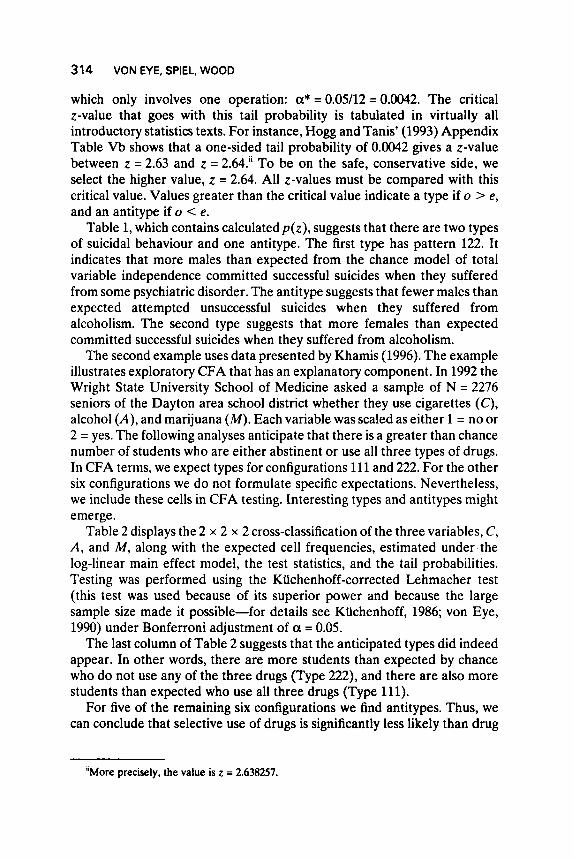
The second example uses data presented by Khamis (1996). The example illustrates exploratory CFA that has an explanatory component. In 1992 the Wright State University School of Medicine asked a sample of N = 2276 seniors of the Dayton area school district whether they use cigarettes (C), alcohol (A) , and marijuana (M). Each variable was scaled as either 1 = no or 2 = yes. The following analyses anticipate that there is a greater than chance number of students who are either abstinent or use all three types of drugs. In CFA terms, we expect types for configurations 111 and 222. For the other six configurations we do not formulate specific expectations. Nevertheless, we include these cells in CFA testing. Interesting types and antitypes might emerge.

Table 2 displays the 2 x 2 x 2 cross-classification of the three variables, C, A, and M, along with the expected cell frequencies, estimated under the log-linear main effect model, the test statistics, and the tail probabilities. Testing was performed using the Kiichenhoff-corrected Lehmacher test (this test was used because of its superior power and because the large sample size made it possible-for details see Kiichenhoff, 1986; von Eye, 1990) under Bonferroni adjustment of a = 0.05.

The last column of Table 2 suggests that the anticipated types did indeed appear. In other words, there are more students than expected by chance who do not use any of the three drugs (Type 222), and there are also more students than expected who use all three drugs (Type 111).

For five of the remaining six configurations we find antitypes. Thus, we can conclude that selective use of drugs is significantly less likely than drug

"More precisely, the value is z = 2.638257.

APPLIED CFA 31 5

TABLE 2 First Order CFA of Drug Use Data

Variables Frequencies Statistics ~

CA M I 0 e Z P ( 4

111 279 64.88 31.12 <a*Type 112 2 47.33 7.34 < a* Antitype 121 456 386.70 5.89 <a*Type 122 44 282.09 21.13 < a* Antitype 21 1 43 124.19 9.75 < a* Antitype 212 3 90.60 11.37 < a* Antitype 22 1 538 740.23 16.06 < a* Antitype 222 91 1 539.98 30.47 < a* Type

'C = Cigarette Use, A = Alcohol Use, M = Marijuana Use

use that follows the all-or-nothing principle. The only exception concerns Configuration 121. It constitutes a type rather than an antitype. Specifically, there are more students than expected who smoke both cigarettes and marijuana but do not consume alcohol. Thus, configuration 121 forms a Type of Exclusively Smoking Students.

2.2 Prediction CFA of Race, Murder, and Verdict

On 11 March 1979, the New York Times Magazine published a cross- tabulation of the three variables, Race of Murderer ( M ; categories: 1 = white, 2 = black), Race of Victim (Vi; categories: 1 = white, 2 = black), and Verdict (V; categories: 1 = death penalty, 2 = other). The published numbers describe murder cases in Florida between 1973 and 1979 (cf Kripendorff, 1986; von Eye, 1991).

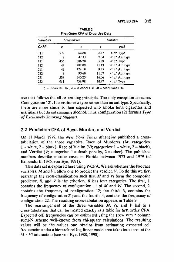
This data set is explored here using P-CFA. We ask whether the two race variables, M and Vi, allow one to predict the verdict, V . To do this we first rearrange the cross-classification such that M and Vi form the composite predictor, R, and V is the criterion. R has four categories. The first, 1, contains the frequency of configuration 11 of M and Vi. The second, 2, contains the frequency of configuration 12; the third, 3, contains the frequency of configuration 21; and the fourth, 4, contains the frequency of configuration 22. The resulting cross-tabulation appears in Table 3.

The rearrangement of the three variables M , Vi, and V led to a cross-tabulation that can be treated exactly as a table for first order CFA. Expected cell frequencies can be estimated using the (row sum * column sum)/N scheme well-known from chi-square calculations. The resulting values will be the values one obtains from estimating expected cell frequencies under a hierarchical log-linear model that takes into account the M x Vi interaction (see von Eye, 1988, 1990).


TABLE 3 P-CFA of Race, Murder, and Verdict

Variables Frequencies Star isrics

R V’ 0 e X’ P(X)

11 12 21 22 31 32 41 42

48 7.89 239 279.1 1

11 61.05 2209 2158.96

72 59.01 2074 2086.99

0 3.05 111 107.95

14.28 2.40 6.41 1.08 1.69 0.28 1.75 0.29

<.oOOl T’

<.oOOl A’ ,008

,141 ,045 ,388 ,040 .384

‘R = Composite Predictor, V = Verdict ’T = Type, A = Antitype

In the present example we select the Bonferroni a-adjustment again and calculate a* = 0.05/8 = 0.00625 for the critical tail probability. The tabulated t-value for this tail probability is between z = 2.49 and z = 2.5”’ (see e.g. Hogg & Tanis, 1993, Appendix Table Vb). The square of this value is the critical X2-value, X 2 = 6.225. We have to use the X2-component test, because two of the expected cell frequencies are less than e = 10. Again, to avoid non-conservative decisions, we decide to go with the larger of the two values thus reducing the threat of committing an a-error even more.

Table 3 which contains the calculated X2-values, suggests the existence of one type and one antitype. The type has pattern 11 or, in terms of the three-variable set-up, pattern 111. This pattern indicates that there are more cases than one would expect from independence between the composite predictor Race and the criterion Verdict in which white murderers of white victims were handed the death penalty.

The antitype has pattern 21 or 121. This pattern suggests that in fewer cases than expected white murderers of black victims were handed the death penalty. Together, the type and antitype pattern of local Race-Verdict relationships suggests that there are statistically significant connections between predictor and criterion categories.

2.3 CFA Symmetry Testing

To illustrate CFA symmetry testing we analyse popularity ratings of N = 86 kindergartners (Spiel, in press). The children attended day care centres in Vienna, Austria. Popularity ratings were given by kindergarten teachers using three-point Likert scales, with “1” indicating low popularity and “3”

“‘More precisely, the value is z = 2.497706.

APPLIED CFA 317

indicating high popularity. These ratings were done twice, the first time one month after entering kindergarten, and the second time six months later.

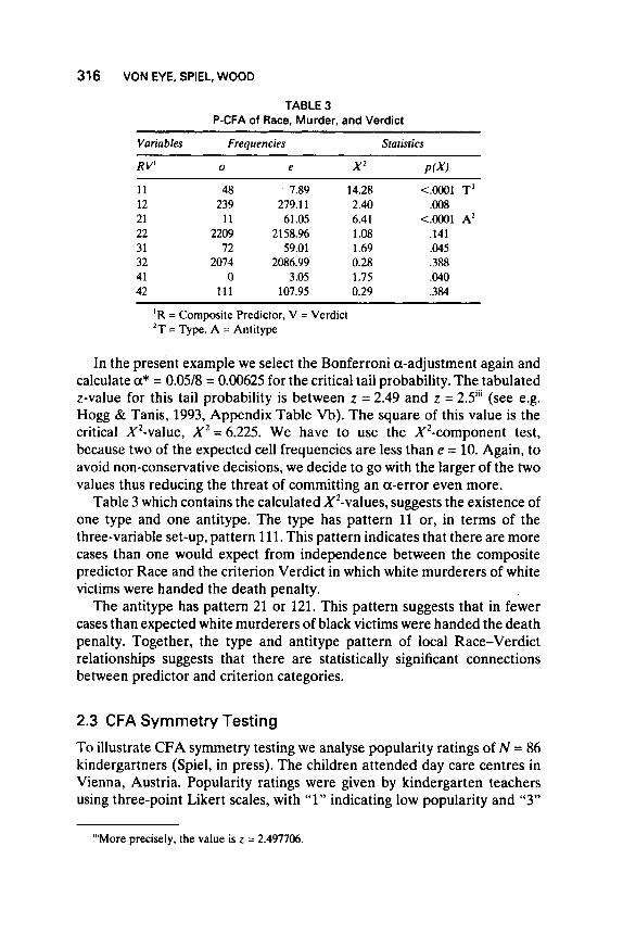
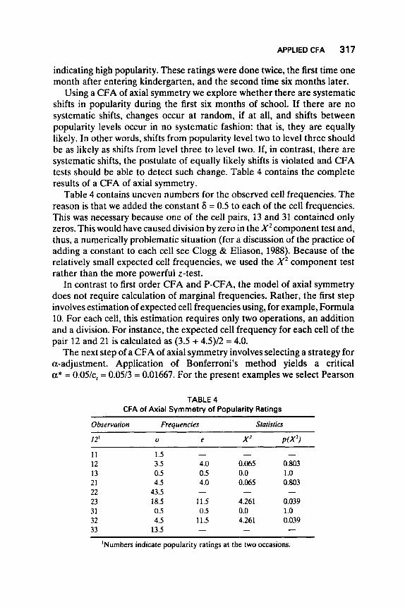
Using a CFA of axial symmetry we explore whether there are systematic shifts in popularity during the first six months of school. If there are no systematic shifts, changes occur at random, if at all, and shifts between popularity levels occur in no systematic fashion: that is, they are equally likely. In other words, shifts from popularity level two to level three should be as likely as shifts from level three to level two. If, in contrast, there are systematic shifts, the postulate of equally likely shifts is violated and CFA tests should be able to detect such change. Table 4 contains the complete results of a CFA of axial symmetry.

Table 4 contains uneven numbers for the observed cell frequencies. The reason is that we added the constant 6 = 0.5 to each of the cell frequencies. This was necessary because one of the cell pairs, 13 and 31 contained only zeros. This would have caused division by zero in the X2 component test and, thus, a numerically problematic situation (for a discussion of the practice of adding a constant to each cell see Clogg & Eliason, 1988). Because of the relatively small expected cell frequencies, we used the X2 component test rather than the more powerful z-test.

In contrast to first order CFA and P-CFA, the model of axial symmetry does not require calculation of marginal frequencies. Rather, the first step involves estimation of expected cell frequencies using, for example, Formula 10. For each cell, this estimation requires only two operations, an addition and a division. For instance, the expected cell frequency for each cell of the pair 12 and 21 is calculated as (3.5 + 4.5)/2 = 4.0.

The next step of a CFA of axial symmetry involves selecting a strategy for a-adjustment. Application of Bonferroni's method yields a critical a* = 0.05/c, = 0.05/3 = 0.01667. For the present examples we select Pearson

TABLE 4 CFA of Axial Symmetry of Popularity Ratings

Observation Frequencies Statistics

12' 0 e X' PW') 11 12 13 21 22 23 31 32 33

1.5 3.5 0.5 4.5

43.5 18.5 0.5 4.5

13.5

- 4.0 0.5 4.0

11.5 0.5

11.5

-

- 0.065 0.0 0.065

4.261 0.0 4.261

- 0.803 1 .o 0.803

0.039 1 .o 0.039

~~~~ ~

'Numbers indicate popularity ratings at the two occasions.


X2 component tests, because the expected cell frequencies are too small for the t-test.

Results suggest neither types nor antitypes. Without adjustment of a the cell pair 23/32 would have defined a type describing a systematic shift by average popularity children towards higher popularity. However, the measures to protect a prevent us from interpreting this possible trend.

2.4 Longitudinal CFA To illustrate longitudinal CFA we use a data set collected to investigate stability and change of performance in school (Spiel, in press). Grades in German in a sample of N = 93'' students were observed at the end of each of the first four elementary school years. Grades were scored as 1 = below average and 2 = above average. Cut-off point was the grand median.

Using Longitudinal CFA we investigate whether there is stability in grades across the first four years in elementary school. The following four variants of types and antitypes can result from application of Longitudinal CFA:

1. Types of Stability. There are two configurations that describe subjects that display no change: 1111 and 2222. If these configurations occur more often than expected from chance, they constitute Types of Stability.

2. Antitypes of Stability. If configurations 1111 and 2222 occur less often than expected from chance, Antitypes of Stability can result.

3. Types of Change. Each of the remaining configurations indicates a pattern of change. Types of Change result if configurations of change occur more often than expected from chance.

4. Antitypes of Change. Change configurations occurring less often than expected from chance can constitute Antitypes of Change.

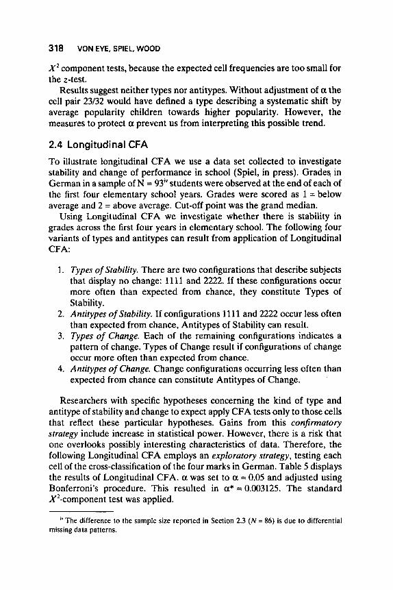
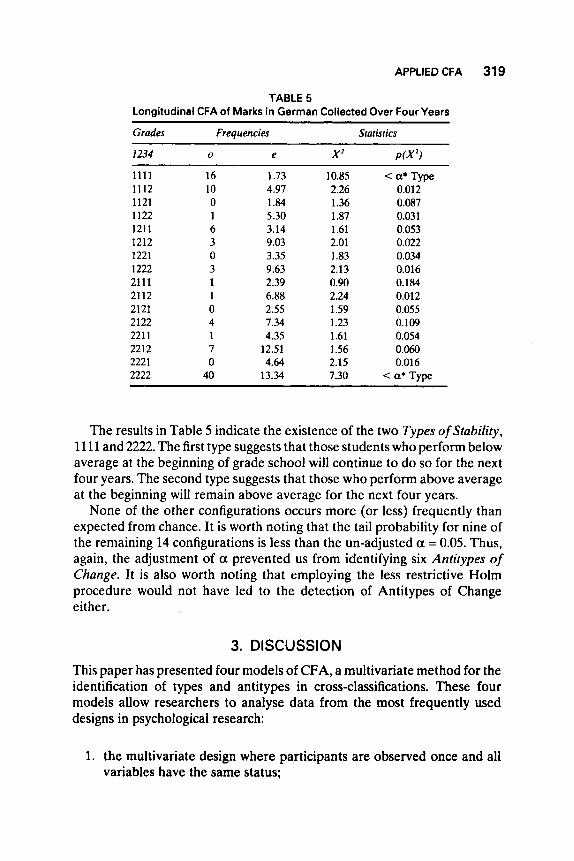
Researchers with specific hypotheses concerning the kind of type and antitype of stability and change to expect apply CFA tests only to those cells that reflect these particular hypotheses. Gains from this confirmatory strategy include increase in statistical power. However, there is a risk that one overlooks possibly interesting characteristics of data. Therefore, the following Longitudinal CFA employs an exploratory strategy, testing each cell of the cross-classification of the four marks in German. Table 5 displays the results of Longitudinal CFA. a was set to a = 0.05 and adjusted using Bonferroni's procedure. This resulted in a* = 0.003125. The standard X2-component test was applied.

'" The difference to the sample size reported in Section 2.3 (N = 86) is due to differential missing data patterns.

APPLIED CFA 31 9

TABLE 5 Longitudinal CFA of Marks in German Collected Over Four Years

Grades Frequencies Statistics

I234 0 e X2 P(X?

1 1 1 1 1112 1121 1122 1211 1212 1221 1222 2111 2112 2121 2122 221 1 2212 2221 2222

16 10 0 1 6 3 0 3 1 1 0 4 1 7 0

40

1.73 4.97 1.84 5.30 3.14 9.03 3.35 9.63 2.39 6.88 2.55 7.34 4.35

12.51 4.64

13.34

10.85 < a* Type 2.26 0.012 1.36 0.087 1.87 0.031 1.61 0.053 2.01 0.022 I .83 0.034 2.13 0.016 0.90 0.184 2.24 0.012 1.59 0.055 1.23 0.109 1.61 0.054 1.56 0.060 2.15 0.016 7.30 < a* Type

The results in Table 5 indicate the existence of the two Types ofStubility, 11 11 and 2222. The first type suggests that those students who perform below average at the beginning of grade school will continue to do so for the next four years. The second type suggests that those who perform above average at the beginning will remain above average for the next four years.

None of the other configurations occurs more (or less) frequently than expected from chance. It is worth noting that the tail probability for nine of the remaining 14 configurations is less than the un-adjusted a = 0.05. Thus, again, the adjustment of a prevented us from identifying six Antitypes of Change. It is also worth noting that employing the less restrictive Holm procedure would not have led to the detection of Antitypes of Change either.

3. DISCUSSION This paper has presented four models of CFA, a multivariate method for the identification of types and antitypes in cross-classifications. These four models allow researchers to analyse data from the most frequently used designs in psychological research:

1. the multivariate design where participants are observed once and all variables have the same status;


2. the multivariate design where participants are observed once and variables differ in status; variables are, for example, predictors and criteria;

3. the univariate repeated measurement design with two observation points; and

4. the uni- or multivariate repeated measurement design with multiple observation points.

Statistical methods for analysis of these designs are plentiful and well-known. For analysis of data from the first design researchers often employ correlational methods, factor analysis, or structural equation modelling. This applies even when data are categorical. For analysis of data from the second design researchers use, for example, regression methods, analysis of variance, path analysis, hierarchical linear models, or structural equation modelling. Again, categorical variables constitute, in principle, no hindrance. For analysis of data from the third design researchers employ, for example, analysis of variance or log-linear methods. For analysis of data from the fourth design, repeated measures analysis of variance or some form of time series analysis are often the methods of choice.

In the canon of these methods, CFA plays a particular role, for four reasons. First, unlike most of the methods listed (exceptions include structural equation modelling and log-linear modelling), CFA allows one to accommodate an extremely wide range of multivariate research designs (for details see Lienert & Krauth, 1974a, b). Second, CFA requires no more than nominal-level variables for analysis. This applies to both predictors and criteria. The only approach that shares this characteristic is log-linear modelling.

Third, CFA is distribution-free; that is, when estimating log-linear chance models, CFA does not use assumptions concerning underlying sample distributions.’ In addition, CFA significance tests do not require that data are sampled from populations with specific distributional characteristics. Therefore, CFA can analyse data even when they do not meet the characteristics required by other, parametric methods. This is of importance in particular in applied research where researchers are often not able to employ experimental designs that guarantee that data have certain characteristics.

Fourth, and most importantly, CFA is a method that allows researchers to pursue the person-oriented approach (also termed profiie-oriented

” Notice, however, that there are approaches to definingparameiric CFA; that is, a method that allows one to use existing distributional parameters when estimating expected cell frequencies (Spiel & von Eye. 1993).

APPLIED CFA 321

approach; Bergman et al., 1991; Magnusson, 1985). While research typically focuses on variables and variable relationships, the person-oriented approach “emphasises the importance of focusing on an information profile or gestalt as the basic piece of information” (Bergman et al., 1991, p.19). Unit of analysis is the profile of individuals’ values. CFA terms these profiles configurations. None of the other methods listed earlier allows one to adopt the person approach.

However, CFA is not the only method that can be applied when operating from the perspective of the person approach. Bergman et al. (1991) mention two groups of methods that, in addition to CFA, provide the researcher with statistical methods for the person approach. These groups include methods of cluster analysis and latent class analysis (LCA). Exploratory CFA as presented in the present paper differs from cluster analysis in that whereas it analyses existing groups of cases, cluster analysis seeks to identify groups of cases. The groups of cases analysed by CFA are defined by their unique patterns of variable indexes. The groups identified by cluster analysis are results of variable associations or density variations.

The difference between LCA and CFA resides in the goals pursued when employing each method. The goal of LCA is to explain observed interactions among manifest variables. A basic assumption of LCA is that there exist two or more types of respondents. Parameters describing these types are optimised with the goal of accounting for observed variable interactions. These types are unobserved: that is, latent. Part of the solution of LCA is that each individual is assigned to one of the latent types. In contrast, CFA does not make comparable assumptions. Types and antitypes are defined at the manifest variable level. No assumptions are made concerning the existence of latent types or dimensions.

One question often of concern is what one can do once types and antitypes have been identified. First and foremost there is theoretical explanation. Applied as well as ivory-tower researchers link the profiles of types and antitypes to existing or emerging theoretical concepts. Types usually indicate that there is a concept, constituted by a pattern of variable states. In contrast, antitypes indicate that there is a group of variable states that do not go together well. Examples of variable states that do not go together well include being simultaneously depressed and in a good mood. One would expect an antitype for this pattern of characteristics.

In addition to theoretical explanation one can attempt external validation of types and antitypes: that is, discrimination using other variables than the ones used for CFA. Open to discussion is the role that those cases play that do not belong to types or antitypes. One option is to define a separate group using these cases. Alternatively, one can focus subsequent analyses on type and antitype members.


Limitations

An often discussed concern raised when application of CFA methods is discussed has to do with the number of cases needed for proper application. To be able to trust results of CFA tests, conditions must be met that largely concern the sample size. Depending on the author one consults, quoted sample size requirements vary widely.

Consider, for example, the Pearson Xz-component test. When reading Weber (1967, p.484; cf Glass & Hopkins, 1984, p.288), one encounters the recommendation that the expected cell frequency must be greater than 5 or 10 for the test statistic Xz to approximate the xz distribution closely enough. It may be on the basis of these recommendations that Krauth and Lienert (1973) put the minimum expected cell frequency for the Xz-test to 5. Over the years, and mostly from simulation studies, requirements have been lowered. Larntz (1978) states that Pearson’s X2-test performs better than other Xz-approximations even when expected cell frequencies are as small as 0.8. Assuming e = 0.8 as the smallest acceptable cell frequency, the minimal sample size for CFA is 0.8c, where c is the number of cells. This minimal number is acceptable, however, only if the expected cell frequency is the same for each cell. Variations are acceptable only if expected cell frequencies are greater than 0.8.

It is important to emphasise that these requirements concern the expected cell frequencies, but not the observed cell frequencies. It is also important to emphasise that performing CFA with sample sizes that small prevents researchers from finding antitypes, because the difference between o = 0 and e = 0.8 cannot be statistically significant.

Similar requirements must be met for the various CFA tests. Some tests, for example, the Lehmacher test (1981), require much larger samples for unbiased testing. In general, one can expect exact tests to require smaller sample sizes than tests that approximate sampling distributions.

Another aspect of sample size considerations concerns the number of variables one can include when applying CFA. CFA applies statistical tests to each cell of a cross-classification. To form this cross-classification one completely crosses the variables under study. As one can imagine, the resulting tables quickly arrive at very large numbers of cells when variables have many categories or when many variables are analysed simultaneously. For example, the analysis of two dichotomous variables creates a cross- classification with 2 x 2 = 4 cells. The analysis of nine dichotomous variables already creates a table with 2’ = 512 cells. Assuming that expected cell frequencies should not be below e = 0.8 we need for this table a sample of N = 410.

However, when compared to alternative statistical methods, CFA does not require larger sample sizes. Log-linear models pose the same

APPLIED CFA 323

requirements. In addition, sample size requirements for General Linear Model applications are often underestimated. For example, a one-factorial ANOVA with three means to compare can detect small size effects with probability greater than 90% only if the sample size is greater than N = 400 (Cohen, 1988).

In sum, CFA has the following characteristics that, taken together, speak to the uniqueness of the method:

1. It allows one to analyse data from a wide range of research designs; 2. it is available in both non-parametric and parametric variants; 3. it is easy to calculate (see Section 2 in the Appendix) and to teach (cf

Aikin et al., 1990); 4. it allows researchers to pursue the person-oriented approach; and 5. it does not pose greater demands on the sample size than other

multivariate methods.

Manuscript received February 1995 Revised manuscript received November 1995

REFERENCES Aikin, L.S., West, S.G., Sechrest, L., Reno, R.R., Roediger, H.L. Ill, Scarr, S., Kazdin, A.E., &

Sherman, S.J. (1990). Graduate training in statistics, methodology, and measurement in psychology: A survey of Ph.D. programs in North America. American Psychologist. 45, 721 -734.

Bergman, L.R., Eklund, G.. & Magnusson, D. (1991). Studying individual development: Problems and methods. In D. Magnusson, L.R. Bergman, G. Rudinger. & B. T6restadt (Eds.), Problems and methods in longitudinal research. Stability and Change (pp.1-27). Cambridge, UK: Cambridge University Press.

Bishop. Y.M.M., Fienberg, S.E., & Holland, P. (1975). Discrete multivariate analysis. Cambridge, MA: MIT Press.

Bowker, A.H. (1948). A test for symmetry in contingency tables. Journal of the American Statistical Association. 43,572-574.

Chipuer, H., & von Eye, A. (1989). Suicide trends in Canada and Germany: An application of Configural Frequency Analysis. Journal of Suicide and Life-Threatening Behavior, 19, 164-1 76.

Clogg, C.C.. & Eliason. S.R. (1988). Some common problems in log-hear analysis. In J.S. Long (Ed.), Common problemdproper solutions. A voiding error in quantitative research (pp.226-257). Newbury Park, CA: Sage.

Clogg, C.C.. Eliason. S.R.. & Grego. J.M. (1990). Models for the analysis of change in discrete variables. In A. von Eye (Ed.), Statistical methods in longitudinal research, Vol. 11: Time series and categorical longitudinal data (pp.409441). Boston. MA: Academic Press.

Cohen. J. (1988). Statisticalpoweranalyis for the behavioralsciences. Hillsdale. NJ: Lawrence Erlbaum Associates Inc.

Emmerich, W. (1968). Personality development and concepts of structure. Child Development. 39.671490.


Glass, G.V.. & Hopkins, K.D. (1984). Statistical methods in education and psychology (2nd

Goodman. L.A. (1978). Analyzing qualitativdcategorical data. Cambridge, MA: Abt Books. Goodman, L.A. (1981). Three elementary views of log-linear models for the analysis of

cross-classifications having ordered categories. Sociological Methods, 191-239. Hecker, H., & Wiese, B. (1994). A mixed model for binary data: The modified X2-test.

Biometrical Journal, 36. 783-799. Heilmann, W.-R., & Schiitt. W. (1985). Tables for binomial testing via F-distribution in

configural frequency analysis. EDV in Biologie und Medizin. 16. 1-7. Hogg, R.V., & Tanis. E.A. (1993). Probability and statistical inference (4th ed.). New York:

Macmillan. Holm, S. (1979). A simple sequentially rejective multiple test procedure. Scandinavian

Journal of Statistics, 6,65-70. Khamis. H.J. (1996). Application of the multigraph representation of hierarchical log-linear

models. In A. von Eye & C.C. Clogg (Eds.), Categorical variables in developmental research (pp. 215-229). Boston: Academic Press.

Krauth, J., & Lienert, G.A. (1973). KFA. Die Konfigurationsfrequenzanalyse und ihre Anwendung in Psychologie und Medizin. Freiburg: Alber.

Krippendorff, K. (1986). Information theory. Structural models for qualitative data. Beverly Hills, CA: Sage.

Kiichenhoff, H. (1986). A note on a continuity correction for testing in three-dimensional contingency tables. Biometrical Journal, 28,465468.

Larntz, K. (1978). Small sample comparisons of exact levels for chi-squared goodness-of-fit statistics. Journal of the American Statistical Association, 73.252-263.

Lehmacher. W. (1981). A more powerful simultaneous test procedure in configural frequency analysis. Biometrical Journal, 23.429436.

Lienert. G.A. (1969). Die “Konfigurationsfrequenzanalyse” als Klassifikationsmethode in der Klinischen Psychologie. In M. Irle (Ed.), Eericht iiber den 26. Kongrej3 der Deutschen Gesellschafi fur Psychologie in Tiibingen 1968 (pp.244-253). Gattingen: Hogrefe.

Lienert. G.A. (1978). Verteilungsfreie Methoden in der Eiostatisrik, Ed. 11. Meisenheim am Glan: Hain.

Lienert, G.A. (1988). Angewandte Konfigurationsfrequenzanalyse. FrankfurUM: Athengum. Lienert, G.A., & Krauth, J. (1974a). Die Konfigurationsfrequenzanalyse X. Auswertung

multivariater klinischer Untersuchungspllne (Teil 1). Zeitschrifi fiir Klinische Psychologie und Psychorherapie, 22.3-1 7.

Lienert. G.A., & Krauth, J. (1974b). Die Konfigurationsfrequenzanalyse XI. Auswertung multivariater klinischer Untersuchungspllne (Teil2). Zeirschrift ffir Klinische Psychologie und fsychorherapie. 22,108-121.

Magnusson, D. (1985). Implications of an interactional paradigm for research on human development. International Journal of Behavioral Development. 8. 115-137.

Perli, H.-G., Hommel, G.. & Lehmacher. W. (1985). Sequentially rejective test procedures for detecting outlying cells in one- and two-sample multinomial experiments. Eiometrical Journal, 27.885-893.

Spiel, C. (in press). Risks to development in infancy pnd childhood Bern: Huber. Spiel, C., & von Eye. A. (1993). Configural Frequency Analysis as a parametric method for

Steiger, J.H., Shapiro, A,. & Browne, M.W. (1985). On the multivariate asymptotic

SYSTAT for Windows. (1992). Statistics. Version 5 Edition. Evanston IL SYSTAT Inc. von Eye. A. (1982). Eeschreibung der Programme “KFA *’ und “THO“ fur Taschenrechner.

ed.). Englewood Cliffs, NJ: Prentice-Hall.

the search for types and antitypes. Biometrical Journal, 35. 151-164.

distribution of sequential chi-square statistics. fsychometrika. 50,253-264.

Unpublished Manual.

APPLIED CFA 325

von Eye, A. (1987). BASIC programs for Configural Frequency Analysis. Unpublished computer programs.

von Eye, A. (1988). The general linear model as a framework for models in configural frequency analysis. Biometrical Journal, 30.5967.

von Eye, A. (1990). Introduction to Configural Frequency Analysis. The search for types and antitypes in cross-classification. Cambridge, UK: Cambridge University Press.

von Eye, A. (1991). Einfiihrung in die Priidiktionsanalyse. In A. von Eye (Ed.), Pradiktionsanalyse. Vorhersagen mit kategorialen Variablen (pp.45-155). Weinheim: Psychologie Verlags Union.

von Eye, A.. & Clogg, C.C. (Eds.) (1996). Categorical variables in developmental research. Boston: Academic Press.

von Eye, A., Kreppner, K., & WeSels, H. (1994). Log-linear modeling of categorical data in developmental research. In D.L. Featherman, R.M. Lerner, & M. Perlmutter (Eds.), Life-span development and behavior, Vol. 12 (pp.225-248). Hillxlale, NJ: Lawrence Erlbaum Associates Inc.

von Eye, A., & Rovine. M.J. (1988). A comparison of significance tests for Configural Frequency Analysis. EDP in Medicine and Biology. 19,613.

von Eye, A,, & Sarensen, S. (1991). Models of chance when measuring interrater agreement with kappa. Biometrical Journal, 39,781 -787.

von Eye, A., & Spiel, C. (1996). Nonstandard log-linear models for measuring change in categorical variables. In A. von Eye & C.C. Clogg (Eds.). Categorical variables in developmental research (pp. 203-214). Boston: Academic Press.

Weber, E. (1967). Grundrg der biologischen Statistik. Jena: Gustav Fischer. Wickens. T.D. (1989). Multivariate contingency tables analysis for the behavioral sciences.

Hillsdale. NJ: Lawrence Erlbaum Associates Inc. Wood, P.K., Sher. K., & von Eye, A. (1994). Conjugate methods in Configural Frequency

Analysis. Biometrical Journal. 36,387410.

TECHNICAL APPENDIX: CALCULATOR AND COMPUTER PROGRAMS FOR CFA

The following technical appendix presents programs to perform CFA using pocket calculators, PCs, or mainframe computers. The first sample program introduced here is aprogram forprogrammablepocket calculators (von Eye, 1982). This program was written for calculators of the HP41 series. The program has the following features:

0 It allows one to analyse up to seven variables simultaneously; 0 all variables must be dichotomous; and 0 it calculates the marginals, the expected frequencies, the Pearson X2

components, Lehmacher test t-values, and the tail probabilities for the t-values.

All the user has to key in is the number of variables and the cell frequencies. Another version of this pocket calculator program computes a second order CFA for three variables. This model considers main effects and pair-wise associations between variables; thus, types and antitypes emerge only if local


higher-order associations among variables exist. This program has the following features:

0 It requires three dichotomous variables; 0 it calculates the marginals, the expected cell frequencies, Pearson X2

components, and the tail probabilities for the X2 values.

Although considerably slower than PC programs, these programs are significantly faster than hand-calculation or calculation using a pocket calculator. In addition, miscalculations are reduced to a minimum.

At the PC and the mainframe level, there are various options for performing CFAs. These options include applications of programs written to do CFA only, and application of general-purpose statistical software to do the steps necessary for CFA. Special CFA programs include von Eye’s (1987) interpreted GW BASIC program. This program has the following features:

0 It can handle up to 100 variables (computer memory permitting); 0 each of the variables can have up to 100 categories; 0 it is interactive within a DOS environment; 0 results are sent to a printer rather than to a screen or file; 0 it gives a choice of eight significance tests; 0 it allows users to choose any significance level; and 0 it performs Bonferroni a-adjustment.

An alternative option involves using log-linear modelling modules of general purpose statistical software packages. For instance, the SY STAT for Windows (1992) TABLES module allows one to estimate any simple log-linear model; that is, any CFA model that can be recast in terms of simple log-linear models. For instance, the first order CFA model discussed in this paper can be treated as a log-linear main effect model. To estimate this model, one requests main effects for each of the variables in a table, except the variable that denotes the frequencies. To get cell-wise test statistics, one requests stundardised residuals which, in SYSTAT, are defined as

o - e ress = 7

These values can be treated as z-values. Alternatives include the following two options:

1. Squaring standardised residuals yields X2 components as defined in (12). Mutiplying e, under the square root with (1 - e /N) yields z-values

APPLIED CFA 327

as defined in (13). The tail probabilities for these values can be looked up in tables and then be compared with the hand-calculated a*.

2. In a similar way, CFA can be performed using the major all-purpose mainframe statistical software packages.

In many of these packages, there may not be the option to print residuals with enough decimals to get precise estimates of tail probabilities for CFA tests. However, in all except marginal cases, program options should be sufficient.

Configural Frequency Analysis as a Method Planned Comparisons in Contingency Table Analysis

Michael J. Rovine, The Pennsylvania State University, USA

Commentary on “Configural Frequency Analysis in Applied Psychological Research” by Alexander von Eye, Christiane Spiel,

and Phillip K. Wood

Configural Frequency Analysis (von Eye, 1990; von Eye, Spiel, & Wood, this issue) represents an excellent strategy for analysing contingency table data in the presence of a very specific hypothesis.

CFA has several advantages over other similar techniques such as prediction analysis (Hildebrand, Laing, & Rosenthal, 1977). First, and probably most important, is that it is intuitively satisfying. An investigator can imagine the cells of a contingency table and impose an hypothesis regarding specific cells. In that sense, CFA bears the same relationship to log-linear analysis as planned comparisons bear to omnibus testing in analysis of variance. Although prediction analysis can accomplish the same ends, as formulated by von Eye (1990), CFA can be more easily linked to the better-known log-linear anlaysis.

Log-linear models test associations in contingency tables by hypothesising a model that yields a set of cell expected values and then pooling the differences between observed and expected values under that null model. The kind of hypothesis tested is: An association exists among a set of variables that represents some level of interaction beyond a specified null model. To test this contribution weighted deviations from the expected value of each cell are calculated and pooled. A significant value of the chi-square statistic does not, of course, mean that the deviations were consistent across cells. A non-significant value of the chi-square statistic does not necessarily mean that interesting things did not happen in a particular cell or in a subset of cells. In the presence of a significant omnibus

configural frequency analysis in applied psychological research

Documents