configurable input devices for 3d interaction using optical tracking … · configurable input...
TRANSCRIPT

Configurable input devices for 3D interaction usingoptical trackingRhijn, van, A.J.
DOI:10.6100/IR616370
Published: 01/01/2007
Document VersionPublisher’s PDF, also known as Version of Record (includes final page, issue and volume numbers)
Please check the document version of this publication:
• A submitted manuscript is the author's version of the article upon submission and before peer-review. There can be important differencesbetween the submitted version and the official published version of record. People interested in the research are advised to contact theauthor for the final version of the publication, or visit the DOI to the publisher's website.• The final author version and the galley proof are versions of the publication after peer review.• The final published version features the final layout of the paper including the volume, issue and page numbers.
Link to publication
General rightsCopyright and moral rights for the publications made accessible in the public portal are retained by the authors and/or other copyright ownersand it is a condition of accessing publications that users recognise and abide by the legal requirements associated with these rights.
• Users may download and print one copy of any publication from the public portal for the purpose of private study or research. • You may not further distribute the material or use it for any profit-making activity or commercial gain • You may freely distribute the URL identifying the publication in the public portal ?
Take down policyIf you believe that this document breaches copyright please contact us providing details, and we will remove access to the work immediatelyand investigate your claim.
Download date: 17. Jul. 2018

Configurable Input Devices for
3D Interaction using Optical Tracking

Copyright c 2006 by Arjen van Rhijn.
All rights reserved. No part of this book may be reproduced, stored in a database or retrieval
system, or published, in any form or in any way, electronically, mechanically, by print, pho-
toprint, microfilm or any other means without prior written permission of the author.
Cover design by Arjen van Rhijn.
Printed by Universiteitsdrukkerij Technische Universiteit Einhoven
CIP-DATA LIBRARY TECHNISCHE UNIVERSITEIT EINDHOVEN
Rhijn, Arjen Jacobus van
Configurable input devices for 3D interaction using optical tracking /
door Arjen Jacobus van Rhijn.
Eindhoven : Technische Universiteit Eindhoven, 2007.
Proefschrift. ISBN 90-386-0834-9. ISBN 978-90-386-0834-1
NUR 980
Subject headings: interactive computer graphics / tracking systems / computer vision / virtual
reality
CR Subject Classification (1998) : I.3.7, I.4.8, H.5.2, I.3.6
Configurable Input Devices for
3D Interaction using Optical Tracking
PROEFSCHRIFT
ter verkrijging van de graad van doctor aan de
Technische Universiteit Eindhoven, op gezag van de
Rector Magnificus, prof.dr.ir. C.J. van Duijn, voor een
commissie aangewezen door het College voor
Promoties in het openbaar te verdedigen
op donderdag 18 januari 2007 om 16.00 uur
door
Arjen Jacobus van Rhijn
geboren te Diemen

Dit proefschrift is goedgekeurd door de promotoren:
prof.dr.ir. R. van Liere
en
prof.dr.ir. J.J. van Wijk
Copromotor:
dr. J.D. Mulder
The research reported in this thesis was carried out at CWI, the Dutch national research in-
stitute for Mathematics and Computer Science, within the theme Visualization and 3D User
Interfaces, a subdivision of the research cluster Information Systems.

TO BARBARA, WHO CARRIES MY HEART
TO MY PARENTS, WHO GAVE ME MY HEART
IN MEMORY OF MIRJAM, WHO WILL ALWAYS BE IN MY HEART

Contents
Contents i
Preface v
1 Introduction 1
1.1 3D Interaction . . . . . . . . . . . . . . . . . . . . . . . . . . . . . . . . . . 2
1.2 Related Work on 3D Interaction Devices . . . . . . . . . . . . . . . . . . . . 5
1.3 Scope . . . . . . . . . . . . . . . . . . . . . . . . . . . . . . . . . . . . . . 7
1.4 Research Objective . . . . . . . . . . . . . . . . . . . . . . . . . . . . . . . 10
1.5 Thesis Outline . . . . . . . . . . . . . . . . . . . . . . . . . . . . . . . . . . 10
1.6 Publications from this Thesis . . . . . . . . . . . . . . . . . . . . . . . . . . 11
2 Model-based Optical Tracking 13
2.1 The Optical Tracking Problem . . . . . . . . . . . . . . . . . . . . . . . . . 13
2.1.1 Problem Statement . . . . . . . . . . . . . . . . . . . . . . . . . . . 14
2.2 Optical Tracking Framework . . . . . . . . . . . . . . . . . . . . . . . . . . 15
2.3 Concepts . . . . . . . . . . . . . . . . . . . . . . . . . . . . . . . . . . . . 17
2.3.1 Camera Model . . . . . . . . . . . . . . . . . . . . . . . . . . . . . 17
2.3.2 Stereo Geometry . . . . . . . . . . . . . . . . . . . . . . . . . . . . 22
2.4 Recognition . . . . . . . . . . . . . . . . . . . . . . . . . . . . . . . . . . . 24
2.4.1 Recognition using 3D features . . . . . . . . . . . . . . . . . . . . . 24
2.4.2 Recognition using 2D Features . . . . . . . . . . . . . . . . . . . . . 25
2.5 Pose Estimation . . . . . . . . . . . . . . . . . . . . . . . . . . . . . . . . . 29
2.5.1 Pose Estimation using Identified 3D Points . . . . . . . . . . . . . . 29
2.5.2 Pose Estimation using Identified 2D Points . . . . . . . . . . . . . . 30
2.5.3 Pose Estimation by Optimization . . . . . . . . . . . . . . . . . . . 31
2.6 The Tracking System of the Personal Space Station . . . . . . . . . . . . . . 31
2.7 Evaluating Tracking Methods . . . . . . . . . . . . . . . . . . . . . . . . . . 33
2.8 Conclusion . . . . . . . . . . . . . . . . . . . . . . . . . . . . . . . . . . . 34
3 Projection Invariant Tracking using Line Pencils 37
3.1 Overview . . . . . . . . . . . . . . . . . . . . . . . . . . . . . . . . . . . . 37
3.2 Concepts . . . . . . . . . . . . . . . . . . . . . . . . . . . . . . . . . . . . 38
3.2.1 Cross Ratio of Line Pencils . . . . . . . . . . . . . . . . . . . . . . 39
3.2.2 Line-to-plane Correspondences . . . . . . . . . . . . . . . . . . . . 40
3.3 Method . . . . . . . . . . . . . . . . . . . . . . . . . . . . . . . . . . . . . 43
3.3.1 Recognition . . . . . . . . . . . . . . . . . . . . . . . . . . . . . . . 45
3.3.2 Pose Estimation . . . . . . . . . . . . . . . . . . . . . . . . . . . . . 46
i

ii Contents
3.3.3 Pose Refinement . . . . . . . . . . . . . . . . . . . . . . . . . . . . 46
3.3.4 Tracking Multiple Devices . . . . . . . . . . . . . . . . . . . . . . . 47
3.4 Results . . . . . . . . . . . . . . . . . . . . . . . . . . . . . . . . . . . . . . 48
3.4.1 Accuracy . . . . . . . . . . . . . . . . . . . . . . . . . . . . . . . . 48
3.4.2 Latency . . . . . . . . . . . . . . . . . . . . . . . . . . . . . . . . . 50
3.4.3 Occlusion . . . . . . . . . . . . . . . . . . . . . . . . . . . . . . . . 51
3.5 Discussion . . . . . . . . . . . . . . . . . . . . . . . . . . . . . . . . . . . . 53
3.5.1 Recognition . . . . . . . . . . . . . . . . . . . . . . . . . . . . . . . 53
3.5.2 Pose Estimation . . . . . . . . . . . . . . . . . . . . . . . . . . . . . 54
3.6 Conclusion . . . . . . . . . . . . . . . . . . . . . . . . . . . . . . . . . . . 55
4 Tracking using Subgraph Isomorphisms 57
4.1 Overview . . . . . . . . . . . . . . . . . . . . . . . . . . . . . . . . . . . . 57
4.2 Marker Tracking . . . . . . . . . . . . . . . . . . . . . . . . . . . . . . . . 60
4.2.1 Stereo Correspondence . . . . . . . . . . . . . . . . . . . . . . . . . 60
4.2.2 Frame-to-frame Correspondence . . . . . . . . . . . . . . . . . . . . 63
4.3 Model Estimation . . . . . . . . . . . . . . . . . . . . . . . . . . . . . . . . 63
4.3.1 Model Definition . . . . . . . . . . . . . . . . . . . . . . . . . . . . 63
4.3.2 Graph Updating . . . . . . . . . . . . . . . . . . . . . . . . . . . . . 64
4.3.3 Reappearing Marker Detection . . . . . . . . . . . . . . . . . . . . . 64
4.3.4 Model Estimation Summary . . . . . . . . . . . . . . . . . . . . . . 67
4.4 Model-based Object Tracking . . . . . . . . . . . . . . . . . . . . . . . . . 68
4.5 Results . . . . . . . . . . . . . . . . . . . . . . . . . . . . . . . . . . . . . . 70
4.5.1 Stereo Correspondence . . . . . . . . . . . . . . . . . . . . . . . . . 71
4.5.2 Model Estimation . . . . . . . . . . . . . . . . . . . . . . . . . . . . 72
4.5.3 Tracking . . . . . . . . . . . . . . . . . . . . . . . . . . . . . . . . 73
4.6 Discussion . . . . . . . . . . . . . . . . . . . . . . . . . . . . . . . . . . . . 74
4.6.1 Marker Tracking . . . . . . . . . . . . . . . . . . . . . . . . . . . . 74
4.6.2 Model Estimation . . . . . . . . . . . . . . . . . . . . . . . . . . . . 75
4.6.3 Model-based Tracking . . . . . . . . . . . . . . . . . . . . . . . . . 75
4.7 Conclusion . . . . . . . . . . . . . . . . . . . . . . . . . . . . . . . . . . . 76
5 Analysis of Tracking Methods 77
5.1 Method . . . . . . . . . . . . . . . . . . . . . . . . . . . . . . . . . . . . . 77
5.1.1 Test Setup . . . . . . . . . . . . . . . . . . . . . . . . . . . . . . . . 78
5.1.2 Performance Metrics . . . . . . . . . . . . . . . . . . . . . . . . . . 80
5.2 Accuracy Model . . . . . . . . . . . . . . . . . . . . . . . . . . . . . . . . . 81
5.2.1 Image Noise . . . . . . . . . . . . . . . . . . . . . . . . . . . . . . 81
5.2.2 Camera Calibration Errors . . . . . . . . . . . . . . . . . . . . . . . 84
5.3 Results . . . . . . . . . . . . . . . . . . . . . . . . . . . . . . . . . . . . . . 87
5.3.1 Accuracy . . . . . . . . . . . . . . . . . . . . . . . . . . . . . . . . 88
5.3.2 Latency . . . . . . . . . . . . . . . . . . . . . . . . . . . . . . . . . 92
5.3.3 Robustness . . . . . . . . . . . . . . . . . . . . . . . . . . . . . . . 93
5.4 Discussion . . . . . . . . . . . . . . . . . . . . . . . . . . . . . . . . . . . . 94
5.5 Conclusion . . . . . . . . . . . . . . . . . . . . . . . . . . . . . . . . . . . 97
6 Analysis of Orientation Filtering and Prediction 99
6.1 Previous Comparisons . . . . . . . . . . . . . . . . . . . . . . . . . . . . . 100

Contents iii
6.2 Filter Parameters . . . . . . . . . . . . . . . . . . . . . . . . . . . . . . . . 100
6.2.1 Framework . . . . . . . . . . . . . . . . . . . . . . . . . . . . . . . 100
6.2.2 Bayesian Filter Parameters . . . . . . . . . . . . . . . . . . . . . . . 101
6.2.3 Motion Models . . . . . . . . . . . . . . . . . . . . . . . . . . . . . 103
6.3 Filter Methods . . . . . . . . . . . . . . . . . . . . . . . . . . . . . . . . . . 104
6.4 Filter Tuning . . . . . . . . . . . . . . . . . . . . . . . . . . . . . . . . . . 107
6.4.1 Measurement Noise Analysis . . . . . . . . . . . . . . . . . . . . . 107
6.4.2 Process Noise Analysis . . . . . . . . . . . . . . . . . . . . . . . . . 108
6.5 Test Procedure . . . . . . . . . . . . . . . . . . . . . . . . . . . . . . . . . 109
6.5.1 Signal characteristics . . . . . . . . . . . . . . . . . . . . . . . . . . 109
6.5.2 Performance Metrics . . . . . . . . . . . . . . . . . . . . . . . . . . 113
6.5.3 System Parameters . . . . . . . . . . . . . . . . . . . . . . . . . . . 114
6.6 Results . . . . . . . . . . . . . . . . . . . . . . . . . . . . . . . . . . . . . . 114
6.6.1 Synthetic Study . . . . . . . . . . . . . . . . . . . . . . . . . . . . . 114
6.6.2 Experimental Study . . . . . . . . . . . . . . . . . . . . . . . . . . . 116
6.7 Discussion . . . . . . . . . . . . . . . . . . . . . . . . . . . . . . . . . . . . 117
6.8 Conclusion . . . . . . . . . . . . . . . . . . . . . . . . . . . . . . . . . . . 123
7 Tracking and Model Estimation of Composite Interaction Devices 125
7.1 Overview . . . . . . . . . . . . . . . . . . . . . . . . . . . . . . . . . . . . 126
7.2 Related Work . . . . . . . . . . . . . . . . . . . . . . . . . . . . . . . . . . 128
7.3 Model Estimation . . . . . . . . . . . . . . . . . . . . . . . . . . . . . . . . 129
7.3.1 Model Definition . . . . . . . . . . . . . . . . . . . . . . . . . . . . 130
7.3.2 Single Marker DOF Relation Estimation . . . . . . . . . . . . . . . . 131
7.3.3 Skeleton Estimation . . . . . . . . . . . . . . . . . . . . . . . . . . 138
7.3.4 Handling Noise . . . . . . . . . . . . . . . . . . . . . . . . . . . . . 140
7.4 Model-based Object Tracking . . . . . . . . . . . . . . . . . . . . . . . . . 141
7.4.1 Single Marker Segment Tracking . . . . . . . . . . . . . . . . . . . 141
7.4.2 Occlusion Handling . . . . . . . . . . . . . . . . . . . . . . . . . . 142
7.5 Results and Discussion . . . . . . . . . . . . . . . . . . . . . . . . . . . . . 142
7.5.1 Model Estimation . . . . . . . . . . . . . . . . . . . . . . . . . . . . 142
7.5.2 Model-based Object Tracking . . . . . . . . . . . . . . . . . . . . . 146
7.6 Conclusion . . . . . . . . . . . . . . . . . . . . . . . . . . . . . . . . . . . 147
8 A Configurable Interaction Device 149
8.1 Introduction . . . . . . . . . . . . . . . . . . . . . . . . . . . . . . . . . . . 149
8.2 Related Work . . . . . . . . . . . . . . . . . . . . . . . . . . . . . . . . . . 151
8.3 CID Construction . . . . . . . . . . . . . . . . . . . . . . . . . . . . . . . . 152
8.4 Parameter Mapping . . . . . . . . . . . . . . . . . . . . . . . . . . . . . . . 153
8.5 Applications . . . . . . . . . . . . . . . . . . . . . . . . . . . . . . . . . . . 158
8.5.1 Modeling . . . . . . . . . . . . . . . . . . . . . . . . . . . . . . . . 158
8.5.2 Manipulation and Data Exploration . . . . . . . . . . . . . . . . . . 158
8.5.3 Animation . . . . . . . . . . . . . . . . . . . . . . . . . . . . . . . 161
8.6 Discussion . . . . . . . . . . . . . . . . . . . . . . . . . . . . . . . . . . . . 162
8.7 Conclusion . . . . . . . . . . . . . . . . . . . . . . . . . . . . . . . . . . . 163
9 Spatial Input Device Structure 165
9.1 Introduction . . . . . . . . . . . . . . . . . . . . . . . . . . . . . . . . . . . 165

iv Contents
9.2 Related Work . . . . . . . . . . . . . . . . . . . . . . . . . . . . . . . . . . 166
9.3 Method . . . . . . . . . . . . . . . . . . . . . . . . . . . . . . . . . . . . . 167
9.3.1 Test Environment . . . . . . . . . . . . . . . . . . . . . . . . . . . . 168
9.3.2 Task Description . . . . . . . . . . . . . . . . . . . . . . . . . . . . 168
9.3.3 Device Configurations . . . . . . . . . . . . . . . . . . . . . . . . . 168
9.3.4 Procedure . . . . . . . . . . . . . . . . . . . . . . . . . . . . . . . . 170
9.3.5 Performance Metrics . . . . . . . . . . . . . . . . . . . . . . . . . . 171
9.4 Results . . . . . . . . . . . . . . . . . . . . . . . . . . . . . . . . . . . . . . 172
9.4.1 Slicing Plane Manipulation Time . . . . . . . . . . . . . . . . . . . 172
9.4.2 Total Task Completion Time . . . . . . . . . . . . . . . . . . . . . . 173
9.4.3 Manipulation Error Chances . . . . . . . . . . . . . . . . . . . . . . 173
9.4.4 Subjective Ratings and Observations . . . . . . . . . . . . . . . . . . 174
9.5 Discussion . . . . . . . . . . . . . . . . . . . . . . . . . . . . . . . . . . . . 176
9.5.1 Motion Type . . . . . . . . . . . . . . . . . . . . . . . . . . . . . . 176
9.5.2 Frame of Reference . . . . . . . . . . . . . . . . . . . . . . . . . . . 176
9.5.3 Intuitiveness versus Comfort . . . . . . . . . . . . . . . . . . . . . . 177
9.5.4 Design Principles . . . . . . . . . . . . . . . . . . . . . . . . . . . . 177
9.6 Conclusion . . . . . . . . . . . . . . . . . . . . . . . . . . . . . . . . . . . 177
10 Conclusion 179
10.1 Contributions . . . . . . . . . . . . . . . . . . . . . . . . . . . . . . . . . . 179
10.2 Future Work . . . . . . . . . . . . . . . . . . . . . . . . . . . . . . . . . . . 181
References 185
Summary 197
Samenvatting 199
Curriculum Vitae 201

Preface
“The most beautiful thing we can experience is the mysterious. It is the source of all
true art and all science. He to whom this emotion is a stranger, who can no longer
pause to wonder and stand rapt in awe, is as good as dead: his eyes are closed.”
Albert Einstein
The events leading up to this thesis began in 2001. After finishing my Master of Science
in Electrical Engineering, I started working for a company where my daily routine consisted
mostly of debugging existing software. Unfortunately, development work in this department
was scarce. Some months later, when the economy was going downhill, rumors started cir-
culating in the company that most of the personnel in my department had to go. Not wanting
to wait for the outcome of these rumors, I started looking around for other work in November
2002.
Coincidentally, my close friend Alexander Scholten worked at the Center for Mathematics
and Computer Science and told me about a Ph.D. position in the field of virtual reality. He
got me into contact with Robert van Liere, who was leading the theme of visualization and
3D user interfaces, and I started working on my Ph.D. in March 2002. Ironically, I always
considered myself more an engineer than a researcher. These events show that there is only
so much a person can plan in his life.
This thesis is the result of several years of research, which would not have been possible
without the help of many people. I would like to express my sincere gratitude to all who
made this work possible and who contributed directly or indirectly.
First of all, many thanks go to my promotors Robert van Liere and Jack van Wijk, and
to my co-promotor and daily supervisor Jurriaan Mulder. The brainstorm sessions with Jur-
riaan often shed new light on the matters at hand, and his knowledge, insights, and creativity
have been a great stimulus during the course of the thesis. The monthly sessions with Jack
always resulted in new ideas and approaches, and they provided a good evaluation of my
own solutions. Jack’s ability to identify problems and generate new and out of the box ideas
has continuously amazed me. The same goes for Robert, who is a walking encyclopedia of
virtual reality literature, who always has a clear vision about where virtual reality is going
and where it should be going, and whose enthusiasm and ability to convey this enthusiasm is
unparalleled.
Special thanks go out as well to the other members of the committee (prof. Berndt
Frohlich, prof. Ulrich Lang, prof. Jean-Bernard Martens, prof. Jos Roerdink) for their
proofreading of the thesis and their valuable comments.
I would also like to thank my colleagues at the visualization and 3D user interfaces
group for the many discussions, both professional and for fun: Breght Boschker, Alexander
Broersen, Chris Kruszynski, Wojciech Burakiewicz, and Ferdi Smit. Furthermore, I would
like to thank the test subjects who voluntarily participated in the user experiments, and Koos
v

vi Preface
van Rhijn and the Technische Verenfabriek De Merwede B.V. for construction help and sup-
ply of materials for the configurable interaction device.
I would like to thank the people that indirectly contributed to this thesis in my personal
life, for their support and for keeping me going. I will always remember the weekly online
sessions with George and Onno, the almost weekly games with Remco and Jen that are now
unfortunately in the past, and the lunches and regular evenings of fun, and probably too much
beer, with Alexander. I hope one day they will excuse me for neglecting them so much in the
last months.
Finally, I especially thank my parents, brother, sister-in-law, and my nieces Tessa and
Mieke, for their invaluable and unconditional support over the years. Last but definitely not
least, I thank Barbara for her love and understanding during my work on this thesis. Thank
you for keeping me sane, focussed, and believing in myself, and for all the beautiful moments,
the joy, and the happiness.
Arjen van Rhijn
Woerden, November 2006

Chapter 1
Introduction
“Interaction in three dimensions is not well understood. Users have difficulty con-
trolling multiple degrees of freedom simultaneously, interacting in a volume rather
than on a surface, and understanding 3D spatial relationships. These problems are
magnified in an immersive virtual environment, because standard input devices such
as mice and keyboards may not be usable...”
Bowman, Johnson, and Hodges, 2001 [BJH01]
In 1965, Ivan Sutherland challenged researchers not to think of a computer monitor as
a screen, but as a window through which one looks into a virtual environment in which the
viewer is immersed [Sut65]. In this environment, users should be able to see, feel, and ma-
nipulate virtual objects as if they were real. Sutherland predicted that advances in computer
science would eventually make it possible to engineer virtual experiences that were convinc-
ing to the human senses.
This vision has driven the field of virtual reality ever since. Advances in display hardware
and software have significantly increased the realism in which virtual objects are presented
to the user, increasing our ability to “see” in a virtual environment. However, increasing
the ability to “feel” and “manipulate” virtual objects still poses a major challenge. In a
survey on the state of the art in virtual reality in 1999, Brooks [Bro99] identified effective
interaction with virtual objects as one of the most crucial issues that needs to be solved, in
order to stimulate the growing success and speed of adoption of virtual reality in real world
applications.
The research in this thesis focusses on 3D interaction in virtual environments. Although
much research has been done on interaction techniques and design methodologies, truly in-
tuitive and natural interaction in virtual environments is still uncommon, and as a result, user
performance is often poor. The reason is that 3D interaction is difficult. As noted by Bowman
et al. [BJH01], users have difficulties understanding 3D spatial relationships and manipulating
3D user interfaces. Conventional interaction paradigms known from the desktop computer,
such as the use of interaction devices as the mouse and keyboard, are insufficient or even
inappropriate for most 3D spatial interaction tasks.
The aim of the research in this thesis is to develop the technology that enables efficient
development of new interaction devices, and which improves 3D user interaction by allowing
interaction devices to be constructed such that their use is apparent from their structure. In
the following sections, the background of the research in this thesis is first reviewed. Next,
the scope is defined and the thesis objective is formulated.
1

2 1. Introduction
Figure 1.1: The interaction process can be modeled as a continuous feedback loop between a
user and a virtual environment.
1.1 3D Interaction
Three-dimensional interaction is an essential part of a virtual environment. The goal of 3D
interaction is to transfer information between a user and a virtual environment. In order
to improve user performance in a virtual environment, interaction should be intuitive and
natural, such that users can focus completely on the task at hand. Users should be able to
perform basic interaction tasks, such as navigating through a 3D environment or selecting
and manipulating virtual objects, as well as more complex tasks that require the manipulation
of a large number of spatial parameters. In the following, we briefly review the 3D interaction
cycle and the aspects that are involved from a cognitive psychology and ergonomics points of
view, as well as from a design methodology and evaluation point of view. Furthermore, the
main issues with 3D interaction are defined.
The Interaction Cycle
The interaction process can be modeled as a continuous cycle, which is symmetric between
the user and the virtual environment. The interaction cycle is depicted in Figure 1.1, which is
adapted from [Mei71]. The user and the virtual environment continuously observe the action
of the other, process and evaluate the observed information, and present new information to
the other party. The user presents information to the system by manipulating user interface
entities, or input devices. The system observes the user’s actions, changes its state as neces-
sary, and defines an appropriate response. The response is fed back to the user by means of
a display system. The user’s perception and cognition system observes the system response,
evaluates the information in the current context, and defines a new action. The user’s context
includes his goals, expectations, and knowledge of the system.
A user’s expectations of the outcome of his actions are influenced by his knowledge about
the system, his experiences with similar actions in the real world, active system feedback, and
passive feedback such as tactile feedback, proprioception and kinesthesis. Proprioception and
kinesthesis enables users to sense the locations and movements of the limbs relative to other
parts of the body.
The main aim in designing 3D interaction is to provide a natural and intuitive interface

1.1. 3D Interaction 3
for the user. This problem has been widely studied in cognitive psychology and ergonomics.
More natural and intuitive interaction can be achieved by minimizing the “gulf of execu-
tion” [HHN86]. The gulf of execution is the difference between a user’s intentions and what
the interaction device allows him to do and how well the system supports his actions. To
minimize the gulf of execution, input devices should be designed such that they enable a user
to perform the actions necessary to complete a task, while minimizing the psychological gap
required to perform these actions.
In this thesis, the geometric arrangement of the degrees of freedom (DOFs) of an input
device is referred to as its spatial structure. It comprises the geometric shape of the device
and the direction of movement of the DOFs relative to the device. A degree of freedom is
defined as the capability of motion in translation or rotation [RDB00]. The spatial structure of
input devices may affect the effectiveness of interaction because of stimulus-response (S-R)
compatibility. S-R compatibility can be defined as the degree to which a response matches
a corresponding stimulus [WB98]. Stimuli and responses are regarded as compatible if they
facilitate efficient action. Various researchers have studied the phenomenon [FS53, BG62,
WB98]. A high level of S-R compatibility is believed to enhance human performance and
reduce cognitive load.
Two aspects of S-R compatibility relate to the spatial structure of input devices: spatial
and directional S-R compatibility. This can be defined as the degree of congruence between
the position and orientation of a device or control and the direction of its motion, and that
of the corresponding visual stimulus [WB98]. Stimulus-response compatibility can be in-
creased by structuring interaction devices such that the user can fully concentrate on the task
that needs to be performed, and not on the operation of the device. As such, an interaction
device should be structured such that it reflects the task at hand. In this case, the structure of
the perceptual and cognition space reflects the structure of the motor space [JS92]. The per-
ception and cognition space arises from the output of the virtual environment and the user’s
expectations and goals, whereas the motor space involves the motor actions a user needs to
perform to manipulate an interaction device.
Design and Development of Effective 3D Interfaces
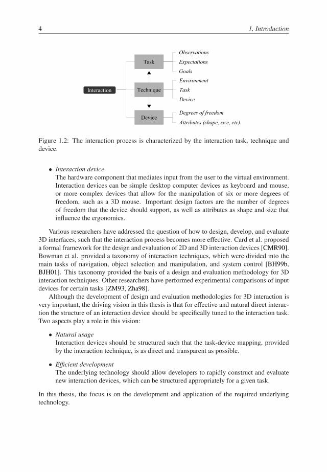
The interaction process is characterized by three aspects, as depicted in Figure 1.2:
� Interaction task
A piece of work that needs to be finished to accomplish a certain goal. The task depends
on a user’s observations of the virtual environment, his expectations, and the goal he
tries to realize (see Figure 1.2). The goal depends on the type of application. For
instance, the goal of applications as architectural design and scientific visualization
may be to gain knowledge of or insight into 3D spatial structures and relationships. To
realize such higher level goals, multiple smaller tasks generally need to be performed,
such as selecting and moving virtual objects.
� Interaction technique
A method by which a user performs a task in the virtual environment, by means of one
or more interaction devices. An interaction technique may be as simple as clicking on
a button, or as complex as performing a specific sequence of operations. An interaction
technique provides a mapping of the functions of an interaction device to the param-
eters of the task to be performed, but is separate from the device. As such, it can be
regarded as an abstraction of the device.
4 1. Introduction
Figure 1.2: The interaction process is characterized by the interaction task, technique and
device.
� Interaction device
The hardware component that mediates input from the user to the virtual environment.
Interaction devices can be simple desktop computer devices as keyboard and mouse,
or more complex devices that allow for the manipulation of six or more degrees of
freedom, such as a 3D mouse. Important design factors are the number of degrees
of freedom that the device should support, as well as attributes as shape and size that
influence the ergonomics.
Various researchers have addressed the question of how to design, develop, and evaluate
3D interfaces, such that the interaction process becomes more effective. Card et al. proposed
a formal framework for the design and evaluation of 2D and 3D interaction devices [CMR90].
Bowman et al. provided a taxonomy of interaction techniques, which were divided into the
main tasks of navigation, object selection and manipulation, and system control [BH99b,
BJH01]. This taxonomy provided the basis of a design and evaluation methodology for 3D
interaction techniques. Other researchers have performed experimental comparisons of input
devices for certain tasks [ZM93, Zha98].
Although the development of design and evaluation methodologies for 3D interaction is
very important, the driving vision in this thesis is that for effective and natural direct interac-
tion the structure of an interaction device should be specifically tuned to the interaction task.
Two aspects play a role in this vision:
� Natural usage
Interaction devices should be structured such that the task-device mapping, provided
by the interaction technique, is as direct and transparent as possible.
� Efficient development
The underlying technology should allow developers to rapidly construct and evaluate
new interaction devices, which can be structured appropriately for a given task.
In this thesis, the focus is on the development and application of the required underlying
technology.

1.2. Related Work on 3D Interaction Devices 5
1.2 Related Work on 3D Interaction Devices
Three-dimensional interaction requires the manipulation of a number of input dimensions.
This can be accomplished by using interaction devices that provide a number of degrees of
freedom, which can be mapped to the input dimensions of the task by the use of an interaction
technique. Interaction tasks can be divided into two categories, based on the number of input
dimensions that need to be manipulated:
� Low dimensional input: Tasks that require the manipulation of up to six input dimen-
sions.
� High dimensional input: Tasks that require the manipulation of more than six input
dimensions.
Low Dimensional Input
In this thesis, low dimensional input tasks are defined as tasks that require the manipulation
of up to six input dimensions. For instance, to change the 3D position and orientation of a
virtual object, three positional and three rotational input dimensions need to be manipulated.
There have been various approaches to designing interaction devices for such tasks. One
approach is to use a standard 2D mouse to perform 3D interaction. However, a mouse has
only two degrees of freedom that can be used to manipulate input dimensions. As such,
positioning and rotating objects in 3D requires the use of an interaction technique that maps
the two degrees of freedom of the mouse to six input dimensions, making interaction more
difficult.
To support more direct 3D interaction, handheld devices have been developed that directly
provide six degrees of freedom (DOFs). Such devices allow for the direct manipulation of
the position and orientation of virtual objects, enabling a user to manipulate virtual objects as
if he was really holding them in his hands.
Many six DOF input devices have been developed, based on different technologies. Ex-
amples of commercially available six DOF input devices are the SpaceBall and the Logitech
6D mouse. The SpaceBall is an input device developed by 3DConnexion [CNX]. It consists
of a rubberized sphere mounted in a base, as illustrated in Figure 1.3(a). An optical sensor is
used to measure six degrees of freedom. It is an isometric rate control device, similar to the
standard desktop mouse. The Logitech 6D mouse is a desktop mouse that has been modified
to provide six DOFs using ultrasonic tracking technology. It is a free flying handheld device
providing direct control over position and orientation. These devices provide a direct and
intuitive interface for controlling the 3D position and orientation of virtual objects.
High Dimensional Input
High dimensional input tasks are defined as tasks that require the manipulation of more than
six input dimensions. For instance, a modeling application may require users to be able to
position, rotate, and scale virtual objects, resulting in nine input parameters. Another example
is a scientific visualization and data analysis application that allows a user to manipulate a
data set and move one or more slicing planes through it. Such applications require complex
spatial 3D interaction.
Two basic approaches for designing interaction devices for high dimensional input tasks can
be distinguished:
6 1. Introduction
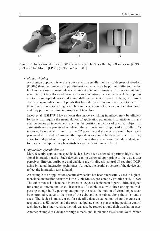
(a) (b) (c)
Figure 1.3: Interaction devices for 3D interaction (a) The SpaceBall by 3DConnexion [CNX],
(b) The Cubic Mouse [FP00], (c) The YoYo [SF03].
� Mode switching
A common approach is to use a device with a smaller number of degrees of freedom
(DOFs) than the number of input dimensions, which can be put into different modes.
Each mode is used to manipulate a certain set of input parameters. This mode switching
may interrupt task flow and present an extra cognitive load on the user. Other options
are to use multiple devices and assign different subtasks to each of them, or to use a
device to manipulate control points that have different functions assigned to them. In
these cases, mode switching is implicit in the selection of a device or a control point,
and may present the same interruption of task flow.
Jacob et al. [JSMC94] have shown that mode switching interfaces may be efficient
for tasks that require the manipulation of application parameters, or attributes, that a
user perceives as independent, such as the position and color of a virtual object. In
case attributes are perceived as related, the attributes are manipulated in parallel. For
instance, Jacob et al. found that the 2D position and scale of a virtual object were
perceived as related. Consequently, input devices should be designed such that they
allow for independent manipulation of attributes that are perceived as independent, and
for parallel manipulation when attributes are perceived to be related.
� Application specific devices
More recently, application specific devices have been designed to perform high dimen-
sional interaction tasks. Such devices can be designed appropriate to the way a user
perceives different attributes, and enable a user to directly control all required DOFs
using bimanual interaction techniques. As such, the spatial structure of the device can
reflect the interaction task at hand.
An example of an application specific device that has been successfully used in high di-
mensional interaction scenarios is the Cubic Mouse, presented by Frohlich et al. [FP00].
The cubic mouse is a handheld interaction device as depicted in Figure 1.3(b), designed
for complex interaction tasks. It consists of a cubic case with three orthogonal rods
passing though it. By pushing and pulling the rods, the motion of virtual objects can
be controlled relative to the pose of the cube and constrained along the x, y, and z
axes. The device is mostly used for scientific data visualization, where the cube cor-
responds to a 3D model, and the rods manipulate slicing planes using position control
techniques. In a later version, the rods can also be rotated around their translation axes.
Another example of a device for high dimensional interaction tasks is the YoYo, which

1.3. Scope 7
was proposed by Simon et al. [SF03]. The YoYo is depicted in Figure 1.3(c). It is a
handheld interaction device, combining elastic force input and isotonic input in a single
unit. The device consists of a cylindric centerpiece, with two rings attached on each
side that can be moved relative to the centerpiece. The rings are used as elastic six DOF
force sensors. The device basically enables a user to control three coordinate systems.
The advantage of developing application specific devices is that they can be designed
appropriate to the way a user perceives different attributes, and that they enable users to di-
rectly control all required degrees of freedom using bimanual interaction. As such, the spatial
structure of the device can reflect the interaction task at hand. In this case, somatosensory
cues that a user receives during device manipulation, such as proprioception and kinesthesis,
are consistent with the visual cues from the virtual environment. Kinesthesis enables users to
feel the movements of their body and limbs, whereas proprioception allows users to sense the
locations of the limbs relative to other parts of the body. The Cubic Mouse is a good example
of a device where these principles are brought into practice.
However, constructing new input devices from scratch for different interaction tasks is
inefficient and impractical. This issue could be solved by developing flexible interfaces that
can easily be configured specifically for a given interaction task. In this thesis, the goal is
to develop configurable interaction devices that allow a designer to rapidly construct and
evaluate new configurations, given the requirements for effective interfaces as discussed in
Section 1.1.
1.3 Scope
The research presented in this thesis was performed using the Personal Space Station (PSSTM)
[ML02, PST]. The PSS is a near-field desktop virtual reality system, which is developed at
CWI. The system is depicted in Figure 1.4. In the PSS, a head tracked user looks into a
mirror in which stereoscopic images are reflected, such that a 3D virtual environment is
created behind the mirror. By using a mirror-based setup, a user can reach under the mirror
and interact with 3D objects without blocking his own projection.
Three-dimensional spatial interaction is performed directly in the virtual environment
with one or more tangible interaction devices. The interaction space is monitored by two
or more cameras. Each camera is equipped with an infrared (IR) pass filter in front of the
lens, and a ring of IR LEDs around the lens to illuminate the interaction space with IR light.
Interaction devices are equipped with retro-reflective markers, which reflect the incoming IR
light back to the cameras.
The PSS uses a model-based optical tracking system. Tracking refers to the process of
measuring the degrees of freedom of an object that moves in a defined space, relative to a
known source [RDB00]. The tracking system is used to recognize the marker configurations
on each interaction device using the images from the cameras, and reconstruct the 3D position
and orientation, or pose, of the devices. By equipping objects with markers, tangible, wireless
input devices can be constructed and tracked in the environment.
The PSS has been used for applications in scientific visualization, and many interaction
techniques have been developed to support these applications. Often, two-handed and high
dimensional interaction is required within the small interaction volume of the PSS. As such,
the PSS imposes the following requirements on the development and use of configurable
interaction devices:

8 1. Introduction
Camera
Mirror
Monitor
VFP
(a) (b)
Figure 1.4: (a) A schematic representation of the Personal Space Station (PSSTM). A user
reaches under a mirror into a virtual environment. The optical tracking system consists of two
or more cameras that are directed to the interaction space. (b) The Personal Space StationTM.
� Small
Devices should be small enough to hold and manipulate comfortably within the inter-
action volume of the PSS.
� Unobtrusive
The use of configurable interaction devices should be unobtrusive. Due to the bimanual
interaction tasks in the small interaction volume of the PSS, this implies that devices
operate without wires.
� Suitable for two-handed interaction
Devices should be constructed such that two-handed interaction and proprioception can
be exploited.
To determine the degrees of freedom of each input device, such as the 3D position and
orientation, the optical tracking system of the PSS needs to be able to recognize which 2D
markers belong to which input device, and estimate the values of the degrees of freedom.
This is done by matching device models to the measured marker locations. These models
describe the 3D configurations of markers on each device. The type of interaction tasks in
the PSS puts the following requirements on a model-based optical tracking system:
� Accurate
The resolution should be better than 1 mm in position and 1 degree in orientation
[WF02].

1.3. Scope 9
� Low latency
The tracking system should be fast enough to track multiple objects with a frame rate
above 60 Hz and a latency below 33 ms. Latency is the effect that a virtual object lags
behind the movements of an input device. Latencies above 33 ms reduce user perfor-
mance and the sense of “being there” in the virtual environment [EYAE99, MRWB03].
� Robust against occlusion
A consequence of optical tracking is that line of sight must be maintained. Many
current optical tracking approaches fail to recognize an input device when one or more
markers become occluded. An optical tracking system should be robust against partial
occlusion of the marker sets.
� Robust against error sources
An optical tracking system should be robust against various error sources. Error sources
include image noise, small camera calibration errors, and errors in the device model.
Undesired effects of error sources include jittering of the virtual object while keeping
the interaction device stationary or failure to recognize an input device.
Additionally, the tracking system should meet the following requirements to allow for ef-
fective development of new interaction devices that are suitable for the high dimensional
interaction tasks in the PSS:
� Generic device shape
Various tracking approaches put constraints on the shape of the objects that can be
tracked, for instance by requiring markers or patterns to be applied to planar surfaces
(e.g. [LM03, KB99, Fia05]). An optical tracking system should be able to track objects
of arbitrary shape.
� Rapid development of devices
It should be easy for a developer to construct new interaction devices by equipping
them with markers. This implies that the application of markers onto the surface of the
device should be an easy procedure. Moreover, in order to construct a new input device,
a developer needs to define a model that describes the 3D locations of markers rela-
tive to the device. Measuring such a model by hand is a tedious and time-consuming
task, and only feasible for objects of simple shape. An optical tracking system should
provide tools to automatically acquire such models.
� Support for configurable interaction devices
Configurable interaction devices enable users to manipulate a large number of input
dimensions. However, most previous tracking approaches focus on tracking standard
six degree of freedom devices. A tracking system should provide tools to assist a
developer in constructing new device configurations, and needs to support tracking of
more than six degrees of freedom.

10 1. Introduction
1.4 Research Objective
The goal of the research in this thesis is defined as follows:
The development and application of configurable input devices for direct 3D
interaction in near-field virtual environments using optical tracking.
The developed concepts and techniques were to be employed in the PSS, a desktop near-
field virtual environment developed at the Center for Mathematics and Computer Science
(CWI). The PSS uses an optical tracking system to measure the 3D position and orientation of
handheld input devices. This system was to be extended to support configurable input devices
and to provide more robust tracking. Although the focus is on desktop near-field VR, the
developed techniques would have to be transferable to different types of virtual environments
as well.
The configurable input devices should:
� Enable users to manipulate large numbers of application parameters with a single, com-
pact device.
� Enable developers to structure devices such that they reflect application parameters,
contributing to intuitive interfaces for high dimensional interaction tasks.
� Enable developers to rapidly develop new interaction techniques and test new configu-
rations.
1.5 Thesis Outline
This thesis is organized as follows. First, a review of the optical tracking field is given in
Chapter 2. The tracking pipeline is discussed, existing methods are reviewed, and improve-
ment opportunities are identified.
In Chapters 3 and 4, we focus on the development of optical tracking techniques of rigid
objects. The goal of the development of the tracking method presented in Chapter 3 is to
reduce the occlusion problem. The method exploits projection invariant properties of line
pencil markers, and the fact that line features only need to be partially visible. The approach
is experimentally compared to a related solution, which is based on projection invariant prop-
erties of point markers.
In Chapter 4, the aim is to develop a tracking system that supports generic device shapes,
and allows for rapid development of new interaction devices. The method is based on sub-
graph isomorphism to identify point clouds, and introduces an automatic model estimation
method that can be used for the development of new devices in the virtual environment. An
experimental comparison is performed to compare the method to a related tracking approach,
which is based on matching 3D distances of point patterns.
Chapter 5 provides an analysis of three optical tracking systems based on different prin-
ciples. The first system is based on an optimization that matches the 3D device model points
to the 2D data points that are detected in the camera images. The other systems are the track-
ing methods as discussed in Chapters 3 and 4. The performance of the tracking methods is

1.6. Publications from this Thesis 11
analyzed, subject to a number of error sources. The accuracy of the methods is analytically
estimated for each of these error sources and compared to experimentally obtained data.
An analysis of various filtering and prediction methods is given in Chapter 6. These
techniques can be used to make the tracking system more robust against noise, and to reduce
the latency problem.
Chapter 7 focusses on optical tracking of composite input devices, i.e., input devices
that consist of multiple rigid parts that can have combinations of rotational and translational
degrees of freedom with respect to each other. Techniques are developed to automatically
generate a 3D model of a segmented input device by moving it in front of the cameras, and
to use this model to track the device.
In Chapter 8, the presented techniques are combined to create a configurable input device,
which supports direct and natural co-located interaction. In this chapter, the goal of the thesis
is realized. The device can be configured such that its structure reflects the parameters of the
interaction task. The interaction technique then becomes a transparent one-to-one mapping
that directly mediates the functions of the device to the task.
In Chapter 9, the configurable interaction device is used to study the influence of spatial
device structure with respect to the interaction task at hand. The driving vision of this thesis,
that the spatial structure of an interaction device should match that of the task, is analyzed
and evaluated by performing a user study.
Finally, in Chapter 10 conclusions are given and future research opportunities are dis-
cussed.
1.6 Publications from this Thesis
Most chapters in this thesis are based on separate publications, which appeared in the pro-
ceedings of international conferences. Chapters 3, 4, 6, 7, 8, and 9 appeared in:
� A. van Rhijn and J. D. Mulder
Optical Tracking using Line Pencil Fiducials
Proceedings of the Eurographics Symposium on Virtual Environments 2004, pp. 35-44.
[RM04]
� A. van Rhijn and J. D. Mulder
Optical Tracking and Calibration of Tangible Interaction Devices
Proceedings of the Workshop on Virtual Environments 2005, pp. 41-50. [RM05]
� A. van Rhijn, R. van Liere, and J. D. Mulder
An Analysis of Orientation Prediction and Filtering Methods for VR/AR
Proceedings of the IEEE Virtual Reality Conference 2005, pp. 67-74. [RLM05]
� A. van Rhijn and J. D. Mulder
Optical Tracking and Automatic Model Estimation of Composite Interaction Devices
Proceedings of the IEEE Virtual Reality Conference 2006, pp. 135-142. [RM06b]
� A. van Rhijn and J. D. Mulder
CID: An Optically Tracked Configurable Interaction Device
Proceedings of Laval Virtual Reality International Conference 2006 [RM06a]

12 1. Introduction
� A. van Rhijn and J. D. Mulder
Spatial Input Device Structure and Bimanual Object Manipulation in Virtual Environ-
ments
Accepted for publication at VRST 2006. [RM06c]
Chapter 5 is based on the following publication:
� R. van Liere and A. van Rhijn
An Experimental Comparison of Three Optical Trackers for Model Based Pose Deter-
mination in Virtual Reality
Proceedings of the Eurographics Symposium on Virtual Environments, pp. 25-34.
[LR04]
During the research of this thesis, various related publications on optical tracking appeared
in the proceedings of international conferences:
� R. van Liere and A. van Rhijn
Search space reduction in optical tracking
Proceedings of the workshop on Virtual environments 2003, pp. 207-214. [LR03]
� J. D. Mulder, J. Jansen, and A. van Rhijn
An Affordable Optical Head Tracking System for Desktop VR/AR Systems
Proceedings of the Workshop on Virtual Environments 2003, pp. 215-223. [MJR03]
� F. A. Smit, A. van Rhijn, and R. van Liere
A Topology Projection Invariant Optical Tracker
Proceedings of the Eurographics Symposium on Virtual Environments 2006, pp. 63-70.
[SRL06]

Chapter 2
Model-based Optical Tracking
In virtual environments, accurate, fast and robust motion tracking of a user’s actions is es-
sential for smooth interaction with the system. Optical tracking has proved to be a valuable
alternative to tracking systems based on other technologies, such as magnetic, acoustic, gy-
roscopic, and mechanical. Advantages of optical tracking include that it is less susceptible to
noise, it allows for many objects to be tracked simultaneously, and interaction devices can be
lightweight and wireless. As such, it allows for almost unhampered operation.
In this chapter, the current state of the art in model-based optical tracking is reviewed.
After defining the aims and problems in optical tracking, various tracking approaches are
discussed and solution strategies reviewed. This chapter focusses on tracking the three-
dimensional position and orientation of rigid interaction devices. Optical tracking techniques
for devices with more degrees of freedom are discussed in Chapter 7.
The chapter is organized as follows. In Sections 2.1 and 2.2, the optical tracking problem
is defined, and a framework is presented that identifies the various steps involved in optical
tracking. In Section 2.3, various concepts are discussed that are used to solve the optical
tracking problem. Sections 2.4 and 2.5 review the most common recognition and pose es-
timation methods. A description of the tracking system of the Personal Space Station as
developed at CWI is given in Section 2.6. Section 2.7 discusses strategies for the evaluation
of tracking methods. Finally, Section 2.8 gives conclusions.
2.1 The Optical Tracking Problem
Optical tracking methods can be divided into two categories:
� Feature-based
Feature-based tracking approaches are based on the detection of certain predefined
features in the environment using imaging sensors. Features are prominent properties
that can be detected in the tracking volume. For instance, colored markers or small
light sources such as light-emitting diodes can be added to a scene. These markers are
relatively easy to find, simplifying the image processing. A common approach is to use
round markers, such that the features are defined by points.
� Vision-based
Vision-based approaches try to identify real-life features by using advanced image
processing. As such, no artificial features need to be introduced to the environment.
Vision-based approaches are generally more computationally expensive than feature-
based approaches. As a consequence, they operate at lower frequency and introduce
higher latency.
13

14 2. Model-based Optical Tracking
Figure 2.1: The coordinate systems involved in the tracking problem.
The research in this thesis focusses on feature-based optical tracking, due to its capability of
achieving high frame rates and low latency.
2.1.1 Problem Statement
Optical tracking of rigid objects can be defined as the measurement of the 3D position and
orientation, or pose, of one or more interaction devices that move in a defined space, relative
to a known location [RDB00]. The tracking problem involves various frames of reference,
as illustrated in Figure 2.1. A frame of reference is represented as a 4�4 homogeneous
transformation matrix [Van94].
The world frame of reference Mworld and the camera frame of reference Mcam are fixed
at an arbitrary location in the tracking space. Features in the camera image are defined in the
image frame of reference Mimg. The transformation MC W that maps camera coordinates to
world coordinates is defined by the extrinsic camera parameters, whereas the transformation
MIC that maps image coordinates to camera coordinates is defined by the intrinsic camera
parameters. These parameters are determined by a camera calibration procedure, which is
discussed in more detail in Section 2.3.1.
The 3D positions, and the orientations if appropriate, of the features on a device are
defined by a device model, which expresses the features in a common model frame Mmodel
that is placed at the origin and aligned with the axes of the interaction device. The model
frame and the world frame are related by a transformation matrix MMW , that, for simplicity
and without loss of generality, can be set to the identity matrix I.
The optical tracking problem can now be formulated as follows:
Determine the matrix Mdev.t/ that transforms the 3D model features in Mmodel
into the world frame Mworld , such that their projections onto the camera image
planes match the detected 2D image features.

2.2. Optical Tracking Framework 15
Figure 2.2: The tracking pipeline and its place in the interaction cycle. Tracking consists of
four subproblems: feature detection, recognition, pose estimation, and filtering and predic-
tion.
2.2 Optical Tracking Framework
In this section, a framework is presented that defines the subproblems that need to be ad-
dressed to solve the optical tracking problem, and how these steps fit within the interaction
cycle as discussed in Chapter 1. The framework also identifies critical parameters that influ-
ence the performance of a tracking method, which are discussed in more detail in Section 2.7.
Figure 2.2 depicts the optical tracking framework and its relation with the interaction
cycle as presented in Figure 1.1. A user performs an action with one or more interaction
devices at time t1. The position and orientation of an input device is represented as the 4�4
homogeneous transformation matrix Mdev.t/. The user’s actions are registered by a tracking
system, which samples the tracking space with a frequency fs and introduces measurement
noise Nz . As a result, the tracking system obtains an estimate OMdev;k at discrete time k of
the actual pose. The pose estimates OMdev;k are used by the virtual environment to update a
simulation, and at time t3 the display is updated accordingly. The time interval t3 � t1 is the
end-to-end latency of the virtual environment.
The first step in optical tracking is feature detection, which involves the application of
image processing techniques to detect the features in the camera images. For instance, if
round markers are used, their 2D locations are detected in the images. Once these features
have been found, the optical tracking problem can be solved in three steps:

16 2. Model-based Optical Tracking
Figure 2.3: Taxonomy of recognition and pose estimation methods.
� Recognition
Recognition involves determining the correspondence between the detected 2D image
features and the 3D features in the device model.
� Pose estimation
Pose estimation entails the calculation of the 3D position and orientation of each input
device.
� Filtering and prediction
The influence of the measurement noise Nz and the effects of latency can be reduced
by the application of filtering and prediction techniques. Such techniques are analyzed
in Chapter 6.
In the following, the recognition and pose estimation steps are discussed in more detail.
Recognition
The recognition problem is defined as the determination of the correspondence between the
detected 2D image features and the 3D markers on the interaction device. This can be accom-
plished by matching the image features to a device model, which describes the 3D structure
of the features on the device relative to the reference frame Mmodel . Recognition methods
can be divided into two categories, as illustrated in Figure 2.3:
� Recognition using 3D features
Features from two or more cameras are first matched to each other to determine the
feature parameters in 3D. The basic steps involve using stereo correspondence to relate
features from one image to the features in a second images, transform these to 3D, and
use a 3D recognition method to identify device features. These steps are discussed in
more detail in Section 2.3.2.
A common approach for recognition using 3D markers is to use point features, such
that recognition can be accomplished in two ways. The first is the geometric hash-
ing approach, which is discussed in Section 2.4.1. The second approach is based on
matching the distances between markers with the distances stored in the device model.
� Recognition using 2D features
Interaction devices are identified completely in 2D using a single camera image. Ex-

2.3. Concepts 17
isting tracking methods generally fall into two categories. The first is to use feature
properties that are invariant under perspective projection. The second approach is to
encode information into planar bitmap patterns. The perspective distortion can easily
be removed from such patterns, such that the encoded information can be retrieved for
recognition.
Previous research that uses these recognition methods are discussed in Section 2.4.
Pose Estimation
Pose estimation is defined as the determination of the 3D position and orientation of the
interaction device, given the correspondence between the data features and the device model
obtained from the recognition step. The most common pose estimation approach is to extract
a set of points from the device model, along with a corresponding set of points from the 2D
image feature set. Three pose estimation approaches can be distinguished:
� Pose estimation using identified 3D points
Points are identified in the recognition step and transformed to 3D space using two or
more cameras. As a result, a set of 3D data points is constructed, along with the set of
corresponding 3D model points. The pose is defined by the transformation that maps
the 3D model points onto the 3D data points.
� Pose estimation using identified 2D points
Points are identified in the recognition step, and a set of 2D data points and the set of
corresponding 3D model points is constructed. The pose is defined by the transforma-
tion that changes the position of the 3D model points such that their projections onto
the image plane match the 2D data points.
� Pose estimation by optimization
In case features cannot be identified, optimization routines can be used to estimate a
pose from the data. In this case, the pose of the input device is iteratively refined to
match the data points to the model.
These approaches are discussed in more detail in Section 2.5.
2.3 Concepts
To solve the optical tracking problem as defined in Section 2.1, the relation between 2D image
features and the world reference frame Mworld needs to be determined. In this section, the
underlying concepts that are needed to solve the optical tracking problem are reviewed.
2.3.1 Camera Model
A camera model defines a mapping between the 3D world and a 2D image. This section
discusses the camera model that is used in the optical tracking techniques presented in this
thesis.

18 2. Model-based Optical Tracking
Figure 2.4: A pinhole camera model, described by its optical center C and its retinal plane
R.
The Pinhole Camera
We first review the most specialized and simple camera model, which is the basic pinhole
camera model. This model is improved upon in the following sections.
A pinhole camera can be described by its optical center C and its retinal plane R. The
retinal plane (or image plane) represents the imaging sensor of the camera, which is generally
a charge-coupled-device (CCD). A 3D point P is projected into an image point p, which is
given by the intersection of the plane R with the line through C and P (see Figure 2.4). The
line through C and the principal point p0, which is orthogonal to R, is called the optical axis.
The distance between C and R is the focal length f .
The relation between a 3D point P and its projection p on the retinal plane R is defined by
a perspective transformation, which is represented by a linear transformation in homogeneous
coordinates. Let the 3D point P and its 2D projection p be expressed as homogeneous
coordinates P D .x; y; z; 1/ and p D .u; v; 1/, respectively. The perspective transformation
is given by
0
@
u0
v0
w0
1
A D MCI MW C
0
B
B
@
x
y
z
1
1
C
C
A
(2.1)
u D u0
w0; v D v0
w0(2.2)
In this equation, the matrix MCI depends solely on intrinsic camera parameters. These are
internal camera parameters, which do not change when adjusting the position and orientation
of the camera, i.e., the principal point p0, the pixel aspect ratio, and the focal length. The
matrix MW C models the extrinsic parameters, which model the position and orientation of
the camera in an arbitrarily fixed world coordinate system.
The camera parameters can be modeled as follows:
� Intrinsic Matrix
In the simplest case of perspective projection, the projection center C is placed at the
origin of the world coordinates and the image plane is aligned with the xy plane, with
the optical axis along the z-axis. This configuration is referred to as camera space.

2.3. Concepts 19
The transformation from a 3D point P D .x; y; z/ to a 2D point p D .u; v/ in camera
space is given by�
u
v
�
D
f xsxzC u0
fysyzC v0
!
(2.3)
where f is the focal length of the camera, s D .sx ; sy/ represents the pixel size along
the u and v axes, and p0 D .u0; v0/ the principal point. In practice, the axes of a pixel
are often not completely orthogonal, which is accounted for by a skew-factor ˛. The
complete matrix MCI from Equation 2.1 is then given by
MCI D
0
B
@
fsx
˛ u0 0
0 fsy
v0 0
0 0 1 0
1
C
A(2.4)
� Extrinsic Matrix
The perspective projection is completely described by the intrinsic matrix, as long as
all coordinates are expressed in camera space. In case the projection center C is not
placed at the origin of the world coordinates and the optical axis does not correspond
to the z-axis, the extrinsic matrix MW C is used to transform points from world space
to camera space. The matrix is defined by a rotation and a translation
MW C D TR (2.5)
Therefore, it is independent of internal camera parameters, and defines the position and
orientation of the camera in world coordinates.
The translation of the world origin to the location of the projection point C D .cx ; cy ; cz/
is defined by the transformation matrix
T D
0
B
B
@
1 0 0 �cx
0 1 0 �cy
0 0 1 �cz
0 0 0 1
1
C
C
A
(2.6)
The rotation matrix R rotates all points around the projection point to align the optical
axis with the z-axis. If the axes of the camera coordinate system are known, this matrix
is given by
R D
0
B
B
@
Nx Ny Nz 0
Ux Uy Uz 0
Vx Vy Vz 0
0 0 0 1
1
C
C
A
(2.7)
where V D .Vx ; Vy ; Vz/ is the camera’s viewing direction, U D .Ux ; Uy ; Uz/ the up
vector, and N D V � U .
Image Distortion
Real cameras deviate from the pinhole model in a few ways, adding non-linear components
to the linear transformation defined by Equation 2.1:

20 2. Model-based Optical Tracking
(a) (b) (c)
Figure 2.5: Illustration of image distortion. (a) The original image. (b) The image with barrel
distortion. (c) The image with pincushion distortion.
� Real camera lenses have a limited depth of field. In order to collect enough light to
expose the CCD, light is gathered across the surface of the lens. As a consequence,
only a small plane in the tracking space is in perfect focus, resulting in a shallow depth
of field. However, by choosing the lens aperture and shutter time appropriately, the
depth of field can be sufficiently increased, such that this effect can be neglected.
� The second cause for deviations from the pinhole model is lens distortion. Due to
various constraints in the lens manufacturing process, the projection of a straight line
on the image plane of a real lens becomes somewhat curved. Since each lens element
is practically radially symmetric, this distortion generally is radially symmetric. This
radial distortion is the most present form of distortion.
Distortion effects can be observed in most cameras, and are generally stronger in wide-angle
lenses. Two types of radial distortion can be distinguished:
� Barrel effect. This type of distortion causes images to appear curved outward from the
center (see Figure 2.5(b)).
� Pincushion effect: this type of distortion causes images to appear pinched towards the
center (see Figure 2.5(c)).
A second form of distortion of tangential distortion. This is due to imperfect centering of the
lens components on the axis and other manufacturing defects.
Lens distortion can be accurately modeled by the sum of the radial and tangential distor-
tions vectors [HS97]. The radial distortion vector is defined as
�
OuOv
�
D�
u.k1r2 C k2r4 C : : :/
v.k1r2 C k2r4 C : : :/
�
(2.8)
where u and v are image coordinates, Ou and Ov are distorted image coordinates, ki are radial
distortion coefficients, and r Dp
u2 C v2.
The tangential distortion vector is defined by
�
OuOv
�
D�
2p1uv C p2.r2 C 2u2/
p1.r2 C 2v2/C 2p2uv
�
(2.9)
where p1 and p2 are tangential distortion coefficients.

2.3. Concepts 21
These equations provide an accurate model to map image coordinates to their distorted
counterparts. However, no analytic solution to the inverse mapping exists [HS97]. A number
of approximative solution strategies exist. One option is to neglect the tangential distortion,
and to invert the parameters of the radial distortion component. Clearly, this approach is not
very accurate. Another option was proposed by Heikkilas, which involves a non-linear search
for implicit parameters to recover the real pixel coordinates from the distorted ones [HS97].
This approach is more accurate than neglecting tangential distortion completely, but is also
more computationally expensive.
Calibration
Camera calibration involves determining the intrinsic and extrinsic camera parameters that
are used in the camera model as discussed in the previous sections. Since the distortion
parameters do not change when moving a camera, they are regarded as intrinsic parameters.
The main idea in calibration is to obtain a number of matching relations between a 3D point
P and its projection p, and use these in an optimization procedure to determine the camera
parameters.
A number of calibration approaches exist, which can be categorized based on the dimen-
sionality of the object used for calibration:
� Three dimensional object calibration
Tsai’s method for camera calibration recovers the intrinsic and extrinsic camera pa-
rameters that provide a best fit of the measured image points to a set of known 3D
target points [Tsa86]. The procedure starts with a closed form least-squares estimate
of some parameters, followed by an iterative non-linear optimization of all parameters
simultaneously. The method works with objects spanning a volume or with coplanar
objects.
� Grid calibration
The most common calibration method uses a coplanar and predefined point grid that
can be moved freely in front of the cameras [Zha00, Tsa86]. At least two images of
the grid have to be taken at different positions and orientations. The main advantage of
this method is that it is relatively easy to construct the calibration object.
� Pointer calibration
Zhang proposed a method that uses a pointer shaped calibration object using collinear
points [Zha02]. The method recovers intrinsic camera parameters. Constraints are
that the object should rotate around a fixed point, and distortion parameters are not
obtained.
� Moving point calibration
In this case, it suffices to move a single point around in the interaction volume [LS00a].
Moving point calibration methods are intended to recover extrinsic parameters only.
Although this is a limitation, a grid calibration method could be used to recover intrin-
sic parameters. Since these parameters remain constant when the camera placement
is changed, extrinsic parameters can be determined using the more convenient moving
point calibration method.

22 2. Model-based Optical Tracking
Figure 2.6: Stereo geometry: A 3D point P is projected onto the image planes of two pinhole
cameras with optical centers C1 and C2.
2.3.2 Stereo Geometry
Many tracking approaches transform the detected image features to 3D by using stereo ge-
ometry. Using stereo geometry, features in two camera images can be matched to each other
and transformed to 3D. This information can then be used to perform the recognition using
3D features.
Consider a stereo setup composed by two pinhole cameras, as illustrated in Figure 2.6.
Let C1 and C2 be the optical centers of the left and right cameras respectively. A 3D point P
is projected onto both image planes, resulting in the 2D point pair p1 and p2. Given p1, its
corresponding point in the right image is constrained to lie on a line called the epipolar line.
The epipolar line is the projection of the optical ray through C1 and p1, and passes through
p2 and e2. All epipolar lines in an image pass through a common point, e1 for the left image
and e2 for the right. This common point is referred to as the epipole, and is the projection of
the optical center of the other camera onto the image plane.
Given a point p1 in one camera image, the search for a corresponding point p2 in the other
camera image is constrained to lie on the epipolar line. A special case is when all epipolar
lines are parallel and horizontal. The search for a corresponding point p2 is then reduced to
a one-dimensional search. This situation occurs when the epipoles e1 and e2 of both images
are at infinity, i.e., when the baseline .C1; C2/ is contained in both focal planes. In this case,
the retinal planes are parallel to the baseline. Any pair of images can be transformed such
that the epipolar lines are parallel and horizontal in each image, as illustrated in Figure 2.7.
This procedure is called rectification.
Rectification involves the following steps:
� Compute the intersection line between the original image planes.
� Compute the baseline .C1; C2/.
� Compute the equation of the plane that is parallel to both lines.
� Rotate both cameras so they have a common orientation.
For a more detailed discussion on stereo geometry and rectification, the reader is referred to
[FP02].

2.3. Concepts 23
Figure 2.7: A stereo setup after rectification. The epipolar lines become horizontal, reducing
the stereo correspondence problem to a one-dimensional search problem.
Stereo Correspondence
The stereo correspondence problem is defined as the determination of the correspondence
between features in the left image and the features in the right image, such that each pair of
features .p1; p2/ originates from the same 3D feature. After rectification, stereo correspon-
dence is reduced to a one-dimensional search problem. Given a feature p1 in one image, its
corresponding feature p2 is constrained to lie on the corresponding horizontal epipolar line.
This search is ambiguous, since multiple features in the right image may lie on the same
epipolar line of a feature in the left image. For instance, in Figure 2.7 the corresponding fea-
ture of p1 is constrained to lie on the epipolar line that passes through p2 and q. As a result,
the 3D point that corresponds to p1 could be either P or Q.
To solve this ambiguity, other matching constraints can be exploited:
� Similarity
Features in both images must have similar attributes and similar neighborhoods.
� Uniqueness
A feature in one image can only correspond to one feature in the other image. An
exception is the case where a feature lies in the same line of view as another feature,
causing them to merge in the camera image.
� Continuity
In case an object contains multiple 3D points relatively close together, the disparity of
corresponding features of the device should vary smoothly. For instance, if a cube is
equipped with markers, the disparity of the 2D projections of the markers on the same
surface varies smoothly. This constraint fails at discontinuities of depth, which cause
abrupt changes in disparity.
� Ordering
If a point p1 in the left image matches a point q1 in the right, a point p2 matches a
point q2, and p1 is to the left of p2, then q1 should also be to the left of q2. In other
worlds, the ordering of features is preserved across images. This constraint can fail in
scenes containing narrow foreground objects [YP84].
Much research has been done on stereo correspondence. Many researchers have ad-
dressed the problem of dense stereo correspondence [SS02], dealing with large numbers of

24 2. Model-based Optical Tracking
features. A common approach is to match features based on the similarity of the surrounding
pixels [PMF85, Pil97, BT98]. Pilu [Pil97] uses an elegant and simple algorithm to incorpo-
rate the uniqueness and similarity constraints into the matching process. He uses a general
correspondence method described by Scott and Longuet-Higgins [SLH91], and defines a sim-
ilarity metric to match features, based on the distance between the 2D feature locations in the
camera images, and the correlation of the surrounding pixels.
Another approach to solve the stereo correspondence problem is to use relaxation tech-
niques. Such techniques use a global matching constraint to eliminate false matches. For in-
stance, Barnard and Thompson [BT80] propose a relaxation technique that starts by assigning
each candidate match a probability value. This value is based on the number of neighboring
matches that have consistent disparity values with the candidate match. The probability value
of each candidate match is iteratively updated until it is below a certain threshold, after which
it is removed. The procedure stops when each candidate match has only one probability value
left, i.e., when all features are in one-to-one correspondence.
Most stereo correspondence approaches use matching metrics such as the correlation of
surrounding pixels or marker characteristics. However, the camera images from the infrared
optical tracking system of the PSS (see Section 2.6), which uses features such as points and
lines, do not contain enough information to use such characteristics. Point or line shaped
markers will have practically identical characteristics in both images. In this case, other
approaches need to be found to solve the stereo correspondence problem.
2.4 Recognition
In the following sections, previous work on recognition approaches as discussed in Sec-
tion 2.2 is reviewed. This overview is not meant to be exhaustive, but rather to review the
most important and practical approaches made in the field of optical tracking. For a more
extensive discussion on optical tracking methods, the reader is referred to [LF05].
2.4.1 Recognition using 3D features
Given a set of 3D data features, the tracking problem can be divided into two steps: matching
a subset of the 3D features to a subset of the features defined in a device model, and deter-
mining the pose of each recognized device. Most trackers based on 3D features use point
shaped markers. These approaches can be divided into two categories:
� Pattern-based methods
These methods subdivide a model into small unique patterns, and try to match complete
patterns with the features found in the camera images. These methods are generally
efficient in terms of computational and storage requirements, but fail to track an object
when patterns are only partially visible.
� Point-cloud based methods
In this case, all points of a model are considered as one whole, and a subset of the
model is matched to the data.

2.4. Recognition 25
Geometric Hashing
A well-known point-cloud based method is geometric hashing [LSW88]. It is based on a
preprocessing stage to generate fast lookup tables. For each combination of three model
points, a coordinate system is defined in which all remaining points are expressed. Next, the
locations of these points are quantized to account for noise, and serve as addresses into a
3D hash table. The table stores pointers back to the model and the reference frame. During
recognition, a combination of three data points is taken and a reference frame is determined.
All other data points are expressed in this frame, and are used to address the hash table
to generate votes for a model and reference frame. If a model receives enough votes, it is
marked as identified. Since the repeated transformation of data points into a reference frame
can be computationally expensive, the effectiveness of this method depends on the amount of
candidates that need to be examined.
3D Distance Methods
Various researchers have used 3D distance fitting approaches for device recognition. An
approach presented by Dorfmuller [Dor99] uses retro-reflective spherical markers on each
input device, which are easily detected as 2D blobs in the camera images. Next, all possible
3D positions are calculated using stereo geometry. Devices are equipped with three markers
to form a non-regular triangle, where all inter-marker distances are unique. A model of a
triangle is then fitted to the 3D data positions by minimizing the sum of differences between
the real markers distances and the measured distances.
Ribo et al. [RPF01] followed a similar approach and used two CCD cameras to track 25
markers in the scene at 30 Hz. The system used Zhang’s calibration method [Zha00], linear
prediction of targets in image space, and straightforward epipolar geometry to determine a
list of candidate 3D marker locations.
Van Liere et al. [LR04] developed a distance-based recognition method that is a special
case of the general Euclidean Distance Matrix completion problem [Lau01], and can be seen
as a generalization of the method proposed by Dorfmuller [Dor99]. The method requires the
definition of point patterns. For each pattern on a device, a distance matrix is constructed by
measuring the 3D distance between each marker pair of the pattern. The recognition method
first finds all the sub-matrices in the data distance matrix D that fit in the pattern distance
matrix P. Then, a least squares fitting metric is used to determine which sub-matrix of D best
fits the pattern distance matrix P.
2.4.2 Recognition using 2D Features
Projection Invariants
Some optical tracking methods use features with projection invariant properties, which are
properties that remain constant under perspective projection. Features with such properties
can be recognized in 2D using a single camera image. In the following, some important
projection invariant properties that have been used for optical tracking are reviewed.
� The Cross Ratio
Projective geometry preserves neither distances nor ratios of distances. However, it
does preserve a property called the cross ratio, which is a ratio of ratios of distances.
Given four collinear points, labeled as A, B, C , D (see Figure 2.8), the cross ratio is

26 2. Model-based Optical Tracking
Figure 2.8: The cross ratio of four collinear points is invariant under perspective projections.
As such, the cross ratio of points A; B; C; D equals the cross ratio of points A0; B0; C 0; D0.
the real number defined by:
Cr .A; B; C; D/ D jABj=jBDjjAC j=jCDj (2.10)
where jABj is the Euclidean distance between points A and B.
The cross ratio has been extended to five coplanar points. Van Liere et al. [LM03] have
applied the cross ratio to construct patterns of four collinear or five coplanar points.
Each device is augmented with one or more patterns, which are modeled and stored
in a database. The model describes the 3D positions of markers on the device in a
common coordinate system, along with the cross ratio of each pattern.
Recognition of patterns is performed by calculating the cross-ratio of each combination
of four or five points detected in the camera image, and by comparing the obtained
cross ratio with a certain range. This range is used to account for noise in the measured
2D marker locations, as the cross ratio is sensitive to noise. The cross ratio and its
associated range of each pattern is obtained by a training procedure, during which a
developer moves the pattern in front of the camera. The resulting values are stored in
the device model.
The computation of the cross ratio depends on the order of the points. Van Liere et al.
[LM03] use a permutation invariant introduced by Meer et al. [MLR98], resulting in a
single cross ratio value, independent of ordering. After recognition, the correspondence
between point patterns in the camera image and the 3D pattern information stored in
the device model is known.
However, to reconstruct the pose of the device, the exact one-to-one correspondence
between individual 2D points and the modeled 3D points has to be known. This cor-
respondence is determined by transforming the points to 3D using stereo geometry,
and calculate the 3D positions of the pattern points. Next, the inter-point distances are
used to match data points to model points, using a least-squares fit metric. For patterns
of five points, this results in a maximum of 25 combinations to test in order to obtain
identified points.
� Graph Topology
Another projection invariant property is graph topology: when projecting a graph struc-
ture its topology remains constant, as long as no parts of the graph become overlayed

2.4. Recognition 27
Figure 2.9: An example device augmented with a graph.
in the camera images. Recent work by Smit et al. [SRL06] exploits this property for
single camera device recognition and pose estimation. Devices are augmented with a
graph, as illustrated in Figure 2.9. This graph can be efficiently located in the camera
images.
The method starts by an image processing stage to retrieve the graph structures in
2D. First, a thresholding method is applied to obtain a binary image. The connected
regions are determined and processed using a morphology-based skeletization algo-
rithm. Small parasitic edges are removed in the final phase. The result is a strictly
4-connected, single pixel width skeleton of the input blobs. The graph topology is ob-
tained by performing a recursive walk method. Vertices are created when a pixel has
more than two neighboring pixels.
The obtained graph topology is matched to a device model, which describes the topol-
ogy and 3D positions of the graph vertices in a common device coordinate system. The
matching is done by applying an error tolerant subgraph matching algorithm, which
is a slight modification of the method by Cordella et al. [CFSV04]. The pose can
be reconstructed using a single camera, although depth resolution is poor. Combining
multiple cameras, a more accurate pose estimate can be obtained.
The approach can handle partial occlusion of the graph structure. Furthermore, recog-
nition is performed entirely in 2D, and therefore no stereo correspondence is needed.
As such, there are virtually no restrictions to camera placement.
� Other projection invariant properties
Various other projection invariant properties have been identified and used for recog-
nition. Verri et al. [VY86] discuss the use of points of zeros of curvature of curves
as projection invariant properties. Mendlovic et al. [MKM90] have used a logarithmic
harmonic filter for projection invariant pattern recognition of bitmap targets. Lui et
al. [LPNC06] have used the projection invariant characteristics of NURBS for stereo
matching.
The applicability of these approaches for tracking in virtual environments, which re-
quire high accuracy and low latency object recognition, is the subject of further re-
search. The use of logarithmic harmonics allows for bitmap patterns to be recognized,
similar to the use of ARToolkit [KB99]. The use of curve shapes may be less suitable
for rapid construction of new interaction devices, unless these curves can be arbitrarily
drawn, printed out, and trained to be recognized by the system.

28 2. Model-based Optical Tracking
(a) (b)
Figure 2.10: (a) Two example ARToolkit bitmap patterns. (b) Two ARTag bitmap patterns
including an error correcting code.
Planar Bitmap Pattern Systems
Planar bitmap pattern systems share ideas with projection invariant properties. They are based
on encoding information into a bitmap that can easily be retrieved after perspective projection.
Planar patterns are used so that the perspective distortion can be accurately removed from the
bitmap and the encoded information can be retrieved.
A widely used framework for augmented reality is ARToolkit [KB99]. This system solves
the recognition problem by detecting a square, planar bitmap pattern, using correlation tech-
niques for pattern recognition. ARToolkit patterns are planar bitmaps and can easily be
printed out and used by the system. Two example patterns are depicted in Figure 2.10(a).
They are enclosed by a black border. Pattern recognition proceeds in two stages: recognition
of the pattern boundaries, and correlation of the interior pattern with the patterns stored in a
database.
The pattern borders are detected by finding connected groups of pixels below a certain
threshold, finding their contours, and marking the contours consisting of four straight lines as
potential patterns. The corners of the contours are used to remove the perspective distortion
and transform the pattern into a canonical coordinate system. Next, an N �N grid is defined
to sample the pattern. The samples are correlated with several reference grids stored in a
pattern file.
The pattern file contains 12 reference grids, which are three versions of four possible ro-
tation positions of a pattern. The three versions are intended to handle different lighting and
distance conditions that influence the appearance of patterns. The system outputs a confi-
dence factor, which is compared to a threshold to determine if a pattern is visible. In case a
pattern has been found, the corners of the border are used to determine the 3D position and
orientation of the pattern using a single camera.
Although ARToolkit is useful for many applications, it has a few disadvantages. First,
it is sensitive to pattern occlusion. In case the border is occluded, the method fails to find
potential patterns, whereas if part of the interior bitmap is occluded the correlation method
fails. Second, the use of correlation methods to recognize patterns causes high false positive
and inter pattern confusion rates.
Fiala [Fia05] reduced the occlusion problem by using an error correcting code as bitmap
pattern in ARTag. It used an edge linking method to detect the pattern borders, instead of the
contour of thresholded images as in ARToolkit. As a result, ARTag can still detect patterns if
part of a border is occluded. The interior pattern is a digitally encoded, error correcting code,
as illustrated in Figure 2.10(b). As a result, the pattern interior may be partially occluded,

2.5. Pose Estimation 29
and ARTag achieves lower false negative rates than ARToolkit, as well as, and more crucially,
lower false positive rates. However, patterns are still required to be planar.
2.5 Pose Estimation
In the following sections, previous work on pose estimation is reviewed. Pose estimation
involves determining the 3D position and orientation of the interaction device, given the data
features and the device model. Pose estimation is usually performed by first extracting a set
of points from the model and image features. In the following, three common approaches are
discussed.
2.5.1 Pose Estimation using Identified 3D Points
If recognition results in identified 3D image points, pose estimation is reduced to the absolute
orientation problem. The absolute orientation problem can be defined as the minimization of
the mean squared error between two matched points sets under rigid-body transformations.
Consider a set of N 3D data points pi and the corresponding model points mi . The goal is to
find the rotation matrix R and translation T that maps mi to pi :
pi D Rmi C T (2.11)
Due to various properties of quaternions that make them preferable over rotation matrices
[Hor87], Equation 2.11 can be expressed as
pi D qmiq�1 C t (2.12)
where q is the quaternion representation of R. The absolute orientation problem can now be
defined as finding the least-squares solution that minimizes the objective function
f .q; t/ DNX
iD1
jpi � qmiq�1 � t j2 (2.13)
over all rotations q and translations t .
Horn [Hor87] derived a solution to the absolute orientation problem. The method can be
summarized by the following steps:
� Calculate the centroids rp and rm of the point sets pi and mi , and subtract these from
the data.
� For each pair of coordinates (pi , mi), calculate all possible products of the point coor-
dinates xpxm, xpym, : : :, zpzm and add these up to obtain Sxx , Sxy , : : :, Szz .
� Compute the elements of the symmetric matrix N
2
4
Sxx C Syy C Szz Syz � Szy Szx � Sxz Sxy � Syx
Syz � Szy Sxx � Syy � Szz Sxy C Syx Szx C Sxz
Szx � Sxz Sxy C Syx �Sxx C Syy � Szz Syz C Szy
Sxy � Syx Szx C Sxz Syz C Szy �Sxx � Syy C Szz
3
5
(2.14)

30 2. Model-based Optical Tracking
� The unit quaternion that minimizes Equation 2.12 is given by the eigenvector that cor-
responds to the most positive eigenvalue of N.
The translation is then given by the difference between the centroid rp and the rotated centroid
r 0m. For the complete derivation of the above procedure, the reader is referred to [Hor87].
2.5.2 Pose Estimation using Identified 2D Points
If recognition results in identified 2D image points, the device pose can be reconstructed
using Quan’s method [QL99]. The idea is to first determine the 3D point locations that
correspond to the 3D model points, given the 2D image points and the camera positions.
Next, the pose estimation problem reduces to the absolute orientation problem as defined
in the previous section, which can be solved efficiently using Horn’s method [Hor87]. The
method for determining the 3D point locations is briefly discussed below.
Given camera calibration matrices MCI and MW C , the camera positions Ci , a set of 2D
image points ui , and a set of corresponding 3D device model points mi , the problem is to
determine the 3D positions pi . Since all pi reside in a different frame of reference as the
device model Mmodel , only the inter-point distances can be used. Each image point ui can
be expressed as a 3D point in the focal plane in world coordinates using the transformation
matrices MIC and MC W , yielding 3D image coordinates Qui . Each 3D point pi is restricted
to lie on the line through the 3D image point Qui and the camera location Ci . The line Li of
point Qui is described by its parametric form Ci C tiDi , with Di D Qui � Ci . To determine
the 3D points that match the model points mi , the distance between each pair of points in the
model (mi , mj ) should match the distance between the corresponding pair of 3D points (pi ,
pj ), such that
dij D jjmi �mj jj2 D jj.Ci C tiDi/ � .Cj C tj Dj /jj2 (2.15)
Algebraic manipulation of this equation results in a polynomial in two unknowns (ti , tj )
fij .ti ; tj / D �dij C .Cij � Cij / � 2.Dj � Cij /tj C .Dj �Dj /t2j
C 2.Di � Cij /ti � 2.Di �Dj /ti tj C .Di �Di/t2i D 0 (2.16)
where Cij D Ci � Cj . The polynomial can be further simplified by normalizing the line
directions Di , such that Di � Di D 1, and by translating all cameras to the origin, such that
Cij D 0. As a result, the following polynomial is obtained
fij .ti ; tj / D t2i C t2
j � 2.Di �Dj /ti tj � dij D 0 (2.17)
Each pair of points leads to an equation of this form. Therefore, given N points, there
are�
N2
�
constraining equations. Using three equations Pij , Pik , and Pjk , a fourth degree
polynomial in t2i can be constructed by variable elimination. Given N points,
�
N �12
�
fourth
degree polynomials in one variable t D t2i can be constructed. For N > 5 this system
is an over-determined homogeneous linear equation system in (1; t; : : : ; t4), which can be
solved in a least-squares fashion by using the singular value decomposition on the�
N �12
�
� 5
coefficient matrix. In case of N D 4 the linear system is under-determined, but can still be
solved (see [QL99] for more details). Therefore, a minimum of four image points ui and its
corresponding model points mi is required to reconstruct the 3D points pi . After calculating
ti , the position of the 3D point pi can be determined using the line equation Ci C tiDi .
After the 3D points pi have been reconstructed, the transformation matrix that maps pi
onto the corresponding 3D model points mi can be determined using Horn’s method [Hor87].
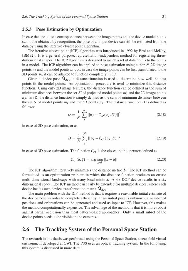
2.6. The Tracking System of the Personal Space Station 31
2.5.3 Pose Estimation by Optimization
In case the one-to-one correspondence between the image points and the device model points
cannot be obtained by recognition, the pose of an input device can still be estimated from the
data by using the iterative closest point algorithm.
The iterative closest point (ICP) algorithm was introduced in 1992 by Besl and McKay,
[BM92]. It is a general purpose, representation-independent method for registering three-
dimensional shapes. The ICP algorithm is designed to match a set of data points to the points
in a model. The ICP algorithm can be applied to pose estimation using either N 2D image
points ui and the model points mi , or, in case the image points can be first transformed to the
3D points pi , it can be adapted to function completely in 3D.
Given a device pose OMdev , a distance function is used to determine how well the data
points fit the model points. An optimization procedure is used to minimize this distance
function. Using only 2D image features, the distance function can be defined as the sum of
minimum distances between the set S 0 of projected model points m0i and the 2D image points
uj . In 3D, the distance function is simply defined as the sum of minimum distances between
the set S of model points mi and the 3D points pj . The distance function D is defined as
follows:
D D 1
N
NX
j
jjuj � Ccp.uj ; S 0/jj2 (2.18)
in case of 2D pose estimation, or as
D D 1
N
NX
j
jjpj � Ccp.pj ; S/jj2 (2.19)
in case of 3D pose estimation. The function Ccp is the closest point operator defined as
Ccp.a; �/ D arg minx2�jjx � ajj (2.20)
The ICP algorithm iteratively minimizes the distance metric D. The ICP method can be
formulated as an optimization problem in which the distance function produces an erratic
multi-dimensional landscape with many local minima. A six DOF device results in a six
dimensional space. The ICP method can easily be extended for multiple devices, where each
device has its own device transformation matrix OMdev .
The main problem with the ICP method is that it requires a reasonable initial estimate of
the device pose in order to complete efficiently. If an initial pose is unknown, a number of
positions and orientations can be generated and used as input to ICP. However, this makes
the method computationally expensive. The advantage of the method is that it is more robust
against partial occlusion than most pattern-based approaches. Only a small subset of the
device points needs to be visible in the cameras.
2.6 The Tracking System of the Personal Space Station
The research in this thesis was performed using the Personal Space Station, a near-field virtual
environment developed at CWI. The PSS uses an optical tracking system. In the following,
this system is discussed in more detail.

32 2. Model-based Optical Tracking
(a) (b)
Figure 2.11: (a) The cameras of the PSS are equipped with infrared-pass filters and a ring of
IR LEDs illuminating the interaction space. (b) An example interaction device. The device
is equipped with retro-reflective markers, which reflect incoming infrared light.
Tracking Setup
The Personal Space Station uses a marker-based optical tracking system. The tracking system
consists of a set of cameras that face the interaction space, as illustrated in Figure 2.11(a). The
PSS uses Leutron Vision LV-7500 progressive scan CCD cameras, operating at a frequency
of 60 Hz. They are connected to a computer, equipped with Leutron Vision PicPort H4D
frame grabbers for synchronized image capturing. More recent versions of the PSS use IEEE
1394 FireWire cameras to reduce the cost of the system.
The interaction space is illuminated by infrared (IR) light using a ring of light-emitting
diodes (LEDs) mounted around the camera lenses. Interaction devices are equipped with
retro-reflective markers, which reflect the incoming IR light back to the cameras. An example
interaction device is given in Figure 2.11(b), where a small wooden cube is shown. By
equipping the lenses with IR-pass filters, the resulting camera images contain the IR light
reflected by interaction device markers, while blocking out most of the background. As a
result, the images contain white blobs corresponding to the markers, which can be located
using simple image processing techniques.
Feature Detection
Feature detection is accomplished by first transforming the camera images to a binary im-
age using a dynamic threshold. Blob candidates are created by finding all distinguishable
connected components using a flood fill method. Next, the center of each blob candidate is
determined using a weighted average of the connected pixels, which is returned as its 2D
position.
Distortion Correction
Distortion correction in the PSS is performed according to the method described by [Rey03].
The approach involves the pre-computation of a 2D lookup table which maps distorted image
coordinates to undistorted coordinates. The lookup table has more pixels than the camera
2.7. Evaluating Tracking Methods 33
images to account for the barrel distortion effect. The idea is then to use bilinear interpolation
to map a distorted point . Ou; Ov/ to a corrected point .u0; v0/. For more details, the reader is
referred to [Rey03].
Calibration
For camera calibration in the PSS, the method of Zhang is used [Zha00]. The method uses
a 2D grid of markers to compute six extrinsic camera parameters (position and orientation),
and eight intrinsic parameters (focal length, aspect ratio, the image center, and two radial and
tangential distortion coefficients).
2.7 Evaluating Tracking Methods
The performance of an optical tracking method can be defined as a combination of three
different factors:
� Accuracy
The accuracy of a tracking method is determined by the difference between the esti-
mated device pose OMdev;k and the real pose Mdev.t/.
� Latency
The latency of a tracking method is defined as the time required for image capturing,
feature detection, recognition, and pose estimation, i.e. t2 � t1 in Figure 2.2.
� Robustness
A tracking method is regarded robust if it satisfies the following properties. First, no
false negatives should occur. Every time the cameras capture an image of an interaction
device, the tracking method should be able to recognize the device and estimate its
pose. Second, no false positives should be reported by the tracking method. If an
interaction device is not located within the interaction volume at a certain time, the
tracking method should not falsely report it. Third, the system should not report an
invalid pose.
The performance of an optical tracking method depends on the reliability of its input param-
eters. From the framework defined in Figure 2.2, four sources of errors can be identified that
influence the input to the tracking methods:
� Lighting conditions
Camera image processing is very sensitive to the lighting conditions. This can lead
to inaccurate parameter values of the detected 2D features, such as inaccurate point
positions or line directions. As a consequence, the device pose estimate exhibits jitter.
� Camera calibration
Inaccurate camera parameters influence the tracking methods in many ways. For ex-
ample, incorrect camera parameters influence stereo geometry computations and the
accuracy of back-projected features, and inaccurate image distortion parameters influ-
ence the geometry of the 2D features.
� Device models
Inaccurate device models influence the recognition and pose estimation procedures,
resulting in a systematic pose estimation error.

34 2. Model-based Optical Tracking
� Occlusion
Occlusion of features can lead to failure to track an interaction device. Additionally,
partially occluded image features may lead to inaccurate feature parameters, leading to
inaccurate device pose estimates.
The performance of optical tracking methods can be evaluated and compared, subject to
each of these error sources. Two evaluation strategies can be distinguished: analytical and
experimental.
An analytical evaluation requires a mathematical analysis of the influence of each of the
steps in the tracking pipeline on the performance metrics, subject to each error source. This
involves creating an accurate model of the lighting conditions, occlusion, camera calibration
errors, and errors in the device model. Next, the accuracy, latency, and robustness of the
complete tracking pipeline have to be mathematically analyzed. This involves performing
an analysis of all parameters that are involved in the feature detection, recognition and pose
estimation methods. A complete analytical evaluation of a tracking method is very complex
and almost infeasible, given the large number of parameters and conditions to be modeled
and analyzed.
An experimental evaluation of tracking methods is less complicated. Two methods can
be experimentally compared under controlled, identical circumstances. There are two ap-
proaches to obtain the device motion sequence that serves as input to the tracking methods.
The first approach is to use a controlled and known motion (e.g. by using a pendulum). The
advantage of this method is that all characteristics of the resulting input signal are known.
However, building a setup with accurately defined motion with respect to the cameras is te-
dious. Furthermore, the resulting motion may be too simple and repetitive to model a realistic
range of motion characteristics, such as the ones encountered in normal interaction scenarios.
The second approach is to let users perform normal interaction tasks. A set of different
motion sequences can be recorded, in which various input parameters to the tracking methods
are varied. Next, accuracy, latency, and robustness metrics can be derived from the data sets.
The disadvantage of experimental evaluations is that it is difficult to control all parameters
that influence the tracking setup, and that trackers may have different relative performance
for different motion sequences. However, by recording a typical interaction task, motion
sequences can be created that feature a variety of motion characteristics to test the tracking
methods. In this thesis, most proposed tracking techniques are evaluated experimentally by
comparing them to a related approach.
2.8 Conclusion
Optical tracking is a powerful method to determine the 3D position and orientation of inter-
action devices. This chapter defined the optical tracking problem and reviewed the state of
the art in object recognition and pose estimation using optical tracking. However, none of
these methods provides the optimal tracking solution.
Given the previous work on optical tracking, four requirements of an optical tracking system
as defined in Chapter 1 need more attention:
� Robustness against occlusion
Most pattern-based methods require an entire pattern to be visible in order to recognize
an object and determine its pose. Point-cloud based methods are better suited to handle

2.8. Conclusion 35
partial occlusion, but are generally less efficient in terms of computational and storage
requirements.
� Generic device shape
Many previous approaches require the application of patterns onto planar surfaces.
However, the development and application of configurable interaction devices requires
that the optical tracking system is able to track objects of arbitrary shape.
� Rapid development of devices
It should be easy for a developer to construct new interaction devices. Some previous
approaches require manual definition of device models, which make it infeasible to
rapidly construct interaction devices of complex shape.
� Support for configurable interaction devices
An optical tracking system should support the use of configurable interaction devices,
which require the tracking of more than six degrees of freedom. Furthermore, the
system needs to provide tools to assist a developer in constructing such devices and
applying them in the virtual environment.

36 2. Model-based Optical Tracking

Chapter 3
Projection Invariant Tracking
using Line Pencils
The previous chapter identified various challenges that should be addressed to make opti-
cal tracking more practical. One of the most limiting properties of optical tracking is that
it requires line-of-sight. In this chapter, the goal is to develop a practical optical tracking
system that is less sensitive to occlusion than conventional point-based tracking methods.
The method is based on projection invariant properties of line pencils, and is experimentally
compared to a related solution using projection invariant properties of point shaped markers.
3.1 Overview
Most conventional point-based optical tracking methods are sensitive to occlusion. If a point
is not visible, the input device often cannot be recognized. Algorithms such as iterative clos-
est point (ICP) [BM92] and geometric hashing [LSW88] are better suited to handle occlusion.
However, geometric hashing generally has large memory requirements and can be too com-
putationally expensive to satisfy the low latency requirement of a practical optical tracking
system as defined in Section 1.3 (objects should be tracked with a frame rate above 60 Hz
and a latency below 33 ms), whereas ICP relies on a good initial estimate for the device pose.
The occlusion problem can be reduced using various strategies:
� Allowing partial occlusion of patterns or marker sets. Various tracking approaches re-
quire a pattern to be visible completely, and cannot combine the information of multiple
partially visible patterns.
� Not requiring individual features to be visible in multiple cameras simultaneously. If
features are required to be visible in multiple cameras, the cameras are required to be
placed close to each other. This may not be optimal with respect to occlusion. Lifting
this restriction results in a tracking method that is better suited to handle occlusion since
less information is needed for recognition and pose estimation, while the cameras can
be placed in a more optimal configuration.
� Using more cameras. Increasing the number of cameras used for recognition and pose
estimation allows for more occlusion per camera. The use of more cameras is more
effective when features do not have to be visible in multiple cameras simultaneously.
In this chapter, the idea is to include these occlusion reduction strategies by relying on pat-
terns of line features, rather than the more common point features. If a line feature becomes
37
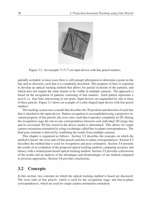
38 3. Projection Invariant Tracking using Line Pencils
Figure 3.1: An example 7�7�7 cm input device with line pencil markers.
partially occluded, in most cases there is still enough information to determine a point on the
line and its direction, such that it is completely described. This property of lines is exploited
to develop an optical tracking method that allows for partial occlusion of the patterns, and
which does not require the same feature to be visible in multiple cameras. The approach is
based on the recognition of patterns consisting of line markers. Each pattern represents a
pencil, i.e. four lines intersecting in one point. Input devices are augmented by one or more
of these pencils. Figure 3.1 shows an example of a cube-shaped input device with line pencil
markers.
The tracking system uses a model that describes the 3D position and direction of each line
that is attached to the input device. Pattern recognition is accomplished using a projective in-
variant property of line pencils, the cross ratio, such that it operates completely in 2D. During
the recognition stage the one-to-one correspondence between each individual 2D image line
and its associated 3D line stored in the device model is determined. This allows for single
camera orientation estimation by using a technique called line-to-plane correspondences. The
final pose estimate is derived by combining the results from multiple cameras.
This chapter is organized as follows. Section 3.2 describes the concepts on which the
method is based: the cross ratio of line pencils and line-to-plane correspondences. Section 3.3
describes the method that is used for recognition and pose estimation. Section 3.4 presents
the results of an evaluation of the proposed optical tracking method, comparing accuracy and
latency with a related point-based optical tracking method. Section 3.5 provides a discussion
of the results and an analysis of the advantages and disadvantages of our method compared
to previous approaches. Section 3.6 provides conclusions.
3.2 Concepts
In this section, two concepts on which the optical tracking method is based are discussed:
The cross ratio of line pencils, which is used for the recognition stage, and line-to-plane
correspondences, which are used for single camera orientation estimation.

3.2. Concepts 39
Figure 3.2: The cross ratio of four collinear points is dual to the cross ratio of four intersecting
lines.
3.2.1 Cross Ratio of Line Pencils
Projective geometry preserves neither distances nor ratios of distances. However, the cross
ratio [FP02], which is a ratio of ratios of distances, remains constant under projective trans-
formations, and can be used to solve the recognition problem in 2D (see Chapter 2).
Figure 3.2 illustrates that the cross ratio of a pencil of four lines is dual to the cross ratio
of four collinear points. It follows from the projection invariant property that the cross ratio
of the intersection points of any arbitrary line L and the lines in the pencil is constant.
The relation between the cross ratio of a pencil of lines and four collinear points can be
obtained as follows. Consider a pencil of four lines passing through an intersection point S .
An arbitrary line L that does not intersect S results in four intersection points A, B, C , and
D. The area of the triangles SAB, SAC , SBD, and SCD can be written as
hjABj=2 D jSAjjSBj sin �12=2 (3.1)
hjAC j=2 D jSAjjSC j sin �13=2 (3.2)
hjBDj=2 D jSBjjSDj sin �24=2 (3.3)
hjCDj=2 D jSC jjSDj sin �34=2 (3.4)
where h is the height of the triangles with respect to L, and �ij is the angle between lines i
and j . Substituting these equations into the cross ratio Equation 2.10 results in
Cr .�12; �13; �34; �24/ D sin �12= sin �24
sin �13= sin �34
(3.5)
yielding an expression for the cross ratio of a line pencil as a function of the angles between
the lines.
From Equations 2.10 and 3.5 some important symmetry properties of the cross ratio can
be derived. These properties imply that a different order of the points (or lines) may result in
the same cross ratio. For example, Cr .A; B; C; D/ D Cr .D; C; B; A/ D Cr .B; A; C; D/.
Furthermore, a uniform scaling of the distances between the points has no influence on the
cross ratio. The consequence of such properties is that there exist pencil configurations with
the same cross ratio.
The cross ratio can be used to identify pencils of four lines in a 2D image, allowing for
single-camera pattern recognition.

40 3. Projection Invariant Tracking using Line Pencils
Figure 3.3: 3D lines Li and their projections li on the image plane I , and the resulting 3D
planes with normals vector Ni .
3.2.2 Line-to-plane Correspondences
Given a 2D line pencil in a camera image and its corresponding 3D pencil model, the geomet-
ric transformation that maps the model onto the 2D image features can be determined. The
situation is illustrated in Figure 3.3. In the figure, a pencil of 3D lines Li is projected onto a
pencil of 2D lines li in the image plane I . Note that line-to-plane correspondence only needs
three lines in a pencil, whereas the recognition method uses four. A line Li is represented by
its parametric equation Li D Oi C tDi , where Oi represents a point on the line, and Di its
direction. The camera’s center of projection C and the line projections li define a sheaf of
planes Vi in 3D, with normal vectors Ni .
After recognition, the problem is to determine the full pose of an input device, given the
center of projection C , the image plane I , the pencil projection li , and the 3D model lines Li .
To accomplish this, the affine transformation matrix M has to be determined that transforms
the model lines into the corresponding planes Vi (see Figure 3.4). This is generally known
as the line-to-plane correspondence problem, and has been addressed by various researchers,
e.g. [CH99, Che91].
The line-to-plane correspondence problem consists of two subproblems: determining po-
sition and determining orientation. The position of the 3D lines must lie on the intersection
line S of the sheaf of planes. The exact position on S cannot be determined from a single
pattern, unless an extra line is used. As such, four unknown degrees of freedom remain: one
translational DOF along line S , and three rotational DOFs. The remaining translational DOF
can be determined using the method described in Section 3.3.2.
To estimate the rotational degrees of freedom, the problem is to find a rotation matrix
R applied to the 3D model lines Li , such that the directions Di are transformed into the
corresponding planes with normals Ni , i.e.
N Ti RDi D 0 (3.6)
Chen [Che91] has addressed the line-to-plane correspondence problem in the general case.
He identified degenerate configurations of lines and planes, for which no solution can be
determined. For valid configurations, he found a closed form solution in the case of three

3.2. Concepts 41
Figure 3.4: The line-to-plane correspondence problem: derive the affine transformation ma-
trix M that transforms the 3D model lines Li into the corresponding planes Vi , given the
center of projection C , the image plane I , and the pencil projection li .
line-to-plane correspondences, resulting in an eight degree polynomial in one unknown.
Chen’s Line-to-plane Correspondence Method
The key of Chen’s method is to first rotate the model lines such that the transformed line L01
lies inside the first plane V1, as illustrated in Figure 3.5. In the resulting configuration, the
line direction D01 is perpendicular to the plane normal N1, and therefore only two rotational
degrees of freedom are left. Chen provides a general solution method to find the remaining
degrees of freedom. In the following, Chen’s method is described in more detail. Next, the
simplifications are given that can be made for configurations of planar line pencils and sheafs
of planes. This leads to an efficient method for determining the orientation of an input device
using a recognized pencil in a single camera.
The first step is to rotate the model lines around axis E D N1 �D1 over an angle �. The
resulting configuration has two rotational degrees of freedom left around the new axes D01
and N1, since these axes have to stay perpendicular. Axis E forms a coordinate system with
N1 and D01 D E �N1, which can be defined to be the x, y, and z axes of a coordinate frame
in which the normals and rotated model lines are expressed. After rotating the lines to this
canonical configuration, the remaining rotation can be written as
R.N1; �/R. OD1; �/ D2
4
cos � 0 sin �
0 1 0
� sin � 0 cos �
3
5
2
4
cos � � sin � 0
sin � cos � 0
0 0 1
3
5 (3.7)
Substituting Equation 3.7 into 3.6 gives a system of equations in cos � , sin � , cos �, and
sin �. This system can be solved using various algebraic manipulations and the fact that
cos2 � C sin2 � D 1. The result is the polynomial in the unknown cos �
P .�/ D8X
iD0
�i cosi � D 0 (3.8)

42 3. Projection Invariant Tracking using Line Pencils
Figure 3.5: The model lines are rotated such that L01 lies inside plane V1. In this config-
uration, two unknown rotations remain: one rotation around L01, and one rotation around
N1.
where the coefficients �i are functions of the components of D2, N2, D3, and N3. The full
derivation of this equation and the coefficients �i are given in [Che91].
Line-to-plane Correspondence for Pencils
In case of line pencils, the lines share an intersection point and are coplanar, and thus the
directions Di D .xi ; yi ; zi/ and the normals Ni D . Nxi ; Nyi ; Nzi/ of the corresponding planes
are both in a coplanar configuration. A canonical configuration is then easily obtained by
applying a rotation RD to orient the lines such that the line directions Di in the yz plane,
such that D1 D .0; 0; 1/, and a rotation RN to orient the normals Ni in the yz plane, such that
N1 D .0; 1; 0/. In the canonical configuration, all x-components of Di and Ni are zero and
cancel out the �i coefficients in Equation 3.8. It can be shown that the resulting polynomial
can be written as
P .�/ D ˛43 � 2˛2
3.˛21 C ˛2
2 C ˛23/ cos2 �
C .2˛21˛2
3 C .˛21 C ˛2
2 C ˛23/2/ cos4 �
� 2˛21.˛2
1 C ˛22 C ˛2
3/ cos6 � C ˛41 cos8 � (3.9)
where
˛1 D �y2 Ny2 Nz3y3 C y2 Nz2 Ny3y3
˛2 D y2 Ny2 Nz3z3 � z2 Nz2 Ny3y3
˛3 D �y2 Nz2 Nz3z3 C z2 Nz2 Nz3y3 (3.10)
Equation 3.9 can be written as a square of fourth-degree polynomials with only a second and
fourth order term. The roots are given by
cos � D ˙
v
u
u
t
B ˙q
B2 � 4˛21˛2
3
2˛21
(3.11)

3.3. Method 43
Figure 3.6: The line-to-plane correspondence problem always has four real solutions for the
pencil case. Two solutions are mirrored versions of the others.
where B D ˛21 C ˛2
2 C ˛23 .
It is worth noting that Equation 3.9 always has four real solutions, since B2 � 4˛21˛2
3 D2˛2
2.˛21 C˛2
3/C .˛21 �˛2
3/2C˛22 > 0, and B �
q
B2 � 4˛21˛2
3 > 0 since B2 > 4˛21˛2
3 > 0.
Therefore, in case the line directions are corrupted by noise, the method is still able to find
a solution. The four solutions are illustrated in Figure 3.6. There are two solutions, Li and
Ki , that lie within the planes bounded by the 2D pencil lines li and the intersection line S .
The other solutions, OLi and OKi , are the reflected pencils that are found since the line-to-plane
correspondence method assumes infinite planes.
After determining cos � and sin � D ˙p
1 � cos2 �, cos � and sin � can be found by
substituting the solutions back into the system of equations defined by 3.7 and 3.6, resulting
in
cos � D ˛1 cos � sin �
˛3 sin �(3.12)
sin � D ˛2 cos �
˛3 sin �(3.13)
The final rotation Rtot is then given by
Rtot D RN R.N1; �/R. OD1; �/RTD (3.14)
3.3 Method
The optical tracking method is based on line pencils. Line pencils are applied to the surface
of each input device, as illustrated in Figure 3.1. The method comprises three stages: recog-
nition, pose estimation, and pose refinement. The tracking pipeline is depicted in Figure 3.7.
The method takes a list of 2D line features detected in a camera image as input, and proceeds
in the following steps:
� Detect all possible pencils of four lines.

44 3. Projection Invariant Tracking using Line Pencils
Figure 3.7: Overview of the tracking pipeline.
� Calculate the cross ratio of each pencil using Equation 3.5.
� Compare the cross ratios to those stored in the device model, and create a list of candi-
date matches.
� Estimate the orientation of the input device using line-to-plane correspondences.
� Estimate the position of the input device from multiple cameras.
� Optimize the pose estimate with respect to all identified pencils.
The 2D line features are detected in the camera images using a straightforward line de-
tection method. Lines are detected by using a dynamic threshold to determine possible line
pixels, after which a flood fill algorithm is performed to detect groups of connected pixels.
Each group of connected pixels defines a possible line. This is similar to the procedure to
detect point features in the camera images, as described in Chapter 2. A 2D line can be
described by its parametric equation
li D pi C tdi (3.15)

3.3. Method 45
where pi represent a position on the line, and di its direction. A position pi is defined by the
center of the connected pixels. The direction di is found by performing a least squares fit of
the line equation to the group of connected pixels, such that the orthogonal distances of the
pixels in the group to the line equation is minimized. If a line is interrupted in the image, for
instance due to occlusion, the line detector return these line segments separately.
3.3.1 Recognition
The recognition stage involves determining the correspondence between the lines detected in
the images and the lines stored in a model database. The model database consists of a list
of pattern models for each input device. Each pattern model consists of four line directions
and the location of the intersection point of the pencil. In the following, each step of the
recognition stage is described in detail.
Pencil Detection
A list of candidate pencils is generated by calculating all line-line intersections, and finding
the intersection points through which at least four lines pass. Intersection points of more than
four lines generate�
N4
�
possible pencil combinations. All these combinations are considered
valid candidate pencils until they are invalidated at a later stage.
Cross Ratio Calculation
The cross ratio of each line pencil that has been detected in the camera images is calculated
according to Equation 3.5. The computation of the cross ratio depends on the order of the
four lines. Since the directions of the lines with respect to their intersection point are known,
the lines are ordered in a clockwise fashion to prevent ambiguities in line order. This results
in only one possible cross ratio for every pencil. The line order is a projection invariant
property, and can be determined by sorting the lines such that
di � dj > 0 8i; j 2 Œ0; 3�; i < j (3.16)
where di represents the line’s direction, and di � dj represents the two-dimensional cross
product. After recognition, the line order can be used to obtain identified lines. If the line
order is not used, recognition would only result in the correspondence between patterns of
2D lines and the associated pattern in the device model, rather than the one-to-one correspon-
dence between the 3D model lines and the 2D image lines. This would result in 4! D 24
possible one-to-one correspondences.
Cross Ratio Check
Changing light conditions, varying illumination of the retro-reflective markers, and miscal-
ibrations all add to image noise, resulting in small variations of the 2D line directions in
each pencil. As the cross ratio function is very sensitive to noise (see [AM95, May95] for
probabilistic analyses of the cross ratio), a training session is included to determine the in-
terval of the cross ratio of each pattern. A device developer moves a pattern around in the
workspace, while the system determines a mean cross ratio and its range of deviations. The
obtained cross ratio of each pattern and its associated range are stored in the model database.
During recognition, all pencils outside the range are not considered candidates for the given

46 3. Projection Invariant Tracking using Line Pencils
pattern. During the training session, colliding ranges of cross ratios are detected to give a
developer feedback on the patterns of the input devices. Typical cross ratio ranges in the PSS
are Cr ˙ 0:025, with Cr the mean cross ratio value obtained during the training session.
3.3.2 Pose Estimation
The pose estimation stage involves calculating the position and orientation of the input device
that has been found in the images.
Orientation Estimation
After recognition, each identified pattern is used to obtain an orientation estimate of the as-
sociated input device. Line-to-plane correspondences are used to calculate possible rotations
of the pattern model, generally resulting in four solutions (see Section 3.2.2). Two of these
solutions can be eliminated, since they fall outside the planes bounded by the 2D pencil lines
li and the intersection line S , as illustrated in Figure 3.6. A valid solution results in the lines
Li , whereas the corresponding invalid solution results in the mirrored lines OLi .
The two remaining rotation solutions can be disambiguated as follows. First, each de-
tected pencil is used to estimate an orientation using line-to-plane correspondences. Next,
the orientation mismatch between each possible pair of pencils in different cameras is deter-
mined. The orientation mismatch follows from the definition of the quaternion as [Sho85]
� D 2 cos�1..q1 � q�12 /w/ (3.17)
where q1, q2 are quaternions representing solutions of a pencil pair, and where qw represents
the w-component of q. As final device rotation matrix Rd, the solution with the smallest
orientation mismatch is selected.
Determining Device Position
The position of a device is determined using two recognized patterns. For this, the two
patterns with the smallest orientation mismatch are used, i.e., the patterns used to derive
the final orientation estimate. First, the vector between the intersection points of these pat-
terns is determined in model coordinates (see Figure 3.8). This vector is transformed by the
rotation matrix Rd, as determined by the line-to-plane correspondence method, giving the
vector W D P1�P2. Next, the line S2 is translated over vector W to S 02, such that its origin
is located at C 02. The position P1 is then given by the intersection point of lines S1 and S 0
2.
3.3.3 Pose Refinement
Pose estimation based on line-to-plane correspondences can produce some jitter in the device
pose, due to noise in the images and thus in the detected 2D line directions. To reduce this
problem, the estimated pose is used as an initial estimate for an optimization procedure.
Pose refinement proceeds in two steps. First, invalid candidate pencils are detected. Sec-
ond, all valid candidate pencils are used in an optimization procedure. The position and ori-
entation of the input device are optimized, such that the angle and distance between the 3D
planes of each identified pencil and the corresponding transformed model lines is minimized.

3.3. Method 47
Figure 3.8: Determining device position.
Invalid Candidate Pattern Detection
After the complete pose of each device is determined, all invalid candidate patterns are identi-
fied from the candidates obtained during recognition. Invalid candidate patterns are detected
by estimating the orientation mismatch between the rotations of each candidate pattern, and
examining the pose estimate of the associated device. If the difference in orientation is larger
than a threshold value, the candidate is invalidated.
Optimization
The pose is optimized to all identified pencils using the downhill simplex method [Chv83].
The downhill simplex method is a commonly used nonlinear optimization algorithm. It is
due to Nelder and Mead [NM65] and is a numerical method for minimizing an objective
function in a multi-dimensional space. It is a direct search, which does not rely on derivative
information, but uses only function evaluations. Given an N dimensional problem, it con-
structs a geometric figure consisting of N C 1 points, which define a simplex. It evaluates a
cost function at the vertices of this simplex, and then iteratively shrinks the simplex as better
solutions are found, until some desired bound is obtained. The method requires a reasonable
initial estimate of the solution.
Note that there are various numeric optimization methods. Although the downhill simplex
method is not the most efficient in terms of the number of function evaluations that it requires,
it is relatively robust and numerically less complicated than most alternatives, and it generally
is able to find reasonably good solutions quickly. Since the initial pose is accurate, this
procedure completes fast.
3.3.4 Tracking Multiple Devices
The tracking method as discussed in the previous sections can be used to track multiple input
devices simultaneously. However, lines from one device may form a pencil with lines from
a second device during recognition. Consequently, many unnecessary candidates are intro-
duced, such that computational requirements are increased and there is a higher likelihood of

48 3. Projection Invariant Tracking using Line Pencils
false pencil matches.
A simple clustering method is performed to reduce the list of candidates. The clustering
method is based on the distance between lines. It assigns lines of different input devices
into separate clusters, unless the devices are very close together with respect to the viewing
direction of the camera. During pencil detection, only lines within a cluster can generate
candidate pencils.
3.4 Results
The pencil-based tracking method has been implemented and evaluated using the PSS. The
accuracy and latency of the method was compared to the point-based tracking method as
presented by [LM03]. This method uses the cross ratio of point patterns for recognition, and
exploits stereo geometry to transform recognized patterns to 3D for pose estimation. Each
pattern consists of 5 coplanar points, applied to the sides of a cubic shaped input device. The
method is described in more detail in Section 2.4.2. For both methods flat retro-reflective
material was used. The point markers have a diameter of 5 mm, whereas the line markers are
approximately 2�45 mm. Both input devices are 7�7�7 cm.
3.4.1 Accuracy
Method
An absolute accuracy study of an optical tracker is a time-consuming and tedious task. The
tracking volume has to be divided into a grid of sufficient resolution. Next, the input de-
vice has to be positioned and oriented accurately at each grid position, after which the pose
estimate from the tracker can be compared to the grid.
The approach of Mulder et al. [MJR03] was followed to obtain a fast indication of the
accuracy. Their approach entails moving the input device over three planes, and collecting the
position measurements from the tracker. Next, for each data set, the measurements are fit to a
plane by minimizing the root-mean-square distance to this plane. The average and maximum
distance of the measurements to the fitted plane give an indication of the positional accuracy
of the tracker.
This approach was extended by including rotation. When moving the input device over
the planes, both position and orientation measurements were collected. Next, the mean angle
between the input device and the fitted plane is determined. The average and maximum
angular deviation of the orientation measurements to the mean angle can then be determined
to give an indication of orientation accuracy.
Results
Figure 3.9 shows the position measurements of both tracking methods for three orthogonal
planes, corresponding to movements of the input device in the xy, xz, and yz planes. The
cameras are placed above the tracking volume, facing down in the direction of the z-axis.
The movement range and speed was similar for both data recordings.
The distance of the measurements to the planes was statistically analyzed to verify that
the data could be approximated by a Gaussian distribution. The t -distribution was used to
determine a 95% confidence interval for the average measurement-to-plane distance [DS98].
Figure 3.10(a) and Table 3.1 summarize the results.

3.4. Results 49
Z
X
Y
Z Z
X
Y
Z
(a)
Z
X
Y
Z Z
X
Y
Z
(b)
Figure 3.9: The 3D data recordings in the xy, xz, and yz planes. Depicted are the recordings
in the tracking volume and the 2D projections of each recording onto its corresponding plane.
(a) Recordings of the tracker based on line patterns. (b) Recordings for the tracker based on
point patterns.
For orientation, the average angular deviation of the measurements with respect to the
mean angle between the input device and the plane is analyzed analogous to the distance of
the measurements to the plane. Figure 3.10(b) and Table 3.2 give the results of the angular
deviations with the 95% confidence intervals.
From these results can be derived that both tracking methods have good accuracy, satis-
fying the 1 mm positional and 1 degree angular accuracy requirements as defined in Chapter
1. An analysis of variance (ANOVA) was performed on the data to indicate statistical signifi-
cance between the tracking methods in the different planes. It was found that the point-based
tracker performs significantly better than the line-based tracker in the xy-plane (F(1,480) =
71.33, p < 0:01). In the xz and yz planes, the line-based tracker performs significantly bet-
ter than the point-based tracker ( F(1,580) = 17.05, p < 0:01 in the xz-plane, and F(1,666)
= 119.31, p < 0:01 in the yz-plane). The line-based tracker performs better in orientation
in all cases (F(1,480) = 17.34, p < 0:01 in the xy-plane, F(1,580) = 99.51, p < 0:01 in the
xz-plane, and F(1,666) = 2372.28, p < 0:01 in the yz-plane). These results suggest that the
line-based tracker has better accuracy in the z-direction (i.e. higher depth resolution) than the
point-based tracking, resulting in better performance in the xz and yz planes.
There are various sources of accuracy differences between both tracking approaches.
First, both methods rely on a model description of each input device. Inaccuracies in these

50 3. Projection Invariant Tracking using Line Pencils
0
0.1
0.2
0.3
0.4
0.5
0.6
0.7
XY line XY point XZ line XZ point YZ line YZ point
Measure
ment-
to-p
lane d
ista
nce (
mm
)
(a)
0
0.2
0.4
0.6
0.8
1
1.2
1.4
XY line XY point XZ line XZ point YZ line YZ point
Angula
r devia
tions (
deg)
(b)
Figure 3.10: Translational and rotational errors for the line-based tracker versus the point-
based tracker. (a) Average measurement-to-plane distances with 95% confidence intervals.
(b) Angular deviations in degrees with 95% confidence intervals.
xy xz yz
Mean 95% Mean 95% Mean 95%
Line 0.37 0.06 0.35 0.08 0.29 0.05
Point 0.22 0.04 0.47 0.08 0.58 0.09
Table 3.1: Measurement-to-plane distances in millimeters with 95% confidence intervals.
xy xz yz
Mean 95% Mean 95% Mean 95%
Line 0.24 0.05 0.34 0.07 0.15 0.04
Point 0.32 0.05 0.64 0.09 1.17 0.07
Table 3.2: Angular deviations in degrees with 95% confidence intervals.
model descriptions translate directly to inaccuracies in the estimated pose. Second, the 2D
features detected from the camera images are different. As the data used for recognition and
pose estimation is different, both methods yield different results in accuracy. As a result, the
use of differently sized point or line markers gives different results.
3.4.2 Latency
The frame rate of both tracking methods was recorded as a function of the number of fea-
tures present in two camera images. Frame rates were measured on a system with a 2.2
GHz Pentium IV CPU and 1 Gb RAM. Both trackers searched for two devices. Figure 3.11
summarizes the results. For both trackers, features were randomly added to the scene and
placed relatively close together, in order to test the worst case situation where no cluster-
ing is performed. An example of a resulting camera image is shown in Figure 3.12. In the
figure, 28 lines have been detected in the image. The recognition stage correctly identified

3.4. Results 51
0
20
40
60
80
100
120
140
160
180
5 10 15 20 25
Number of features
Fra
me
s p
er
se
co
nd
(fp
s)
Point-based Line-based
Figure 3.11: Frame rate measurements of the line-based tracker versus the point-based
tracker, as a function of the number of 2D image features N . Measured using two cameras.
4 pencil patterns. The frame rate for this situation was 67 fps. The frame rate represents
the total tracking time, including detection of 2D features in both camera images. Point and
line detection in the camera images took about 7-9 ms of the total tracking time. The extra
computational cost of line detection compared to point detection is approximately 2 ms.
From Figure 3.11 can be derived that the point-based method becomes infeasible for
more than 15 features, a relatively low number. In contrast, the performance of the line-based
method almost decreases linearly with the number of features and maintains high frame rates.
The performance issues of the point-based tracker are due to the following. First, the line
tracker can reject combinations of four lines that do not form a pencil at a very early stage.
However, the point tracker has to test each combination of five points, and has to use stereo
geometry to transform an identified pattern to 3D, before testing whether the combination of
points is planar. Second, the point tracker can only determine the correspondence between a
pattern of 2D points and the associated pattern in the device model after recognition, whereas
the line tracker has the exact one-to-one correspondence of each data line and its associated
line in the device model. In the point-based tracker, pose estimation is performed by first
transforming the points of the identified pattern to 3D using stereo geometry. Next, the convex
hull of the pattern points is determined, which are matches to the modeled pattern points using
a least squares 3D distance fit metric. For patterns of five points, this results in a maximum
of 25 possible matches.
3.4.3 Occlusion
One of the main advantages of the pencil-based tracking method is its ability to handle con-
siderable amounts of occlusion. Figure 3.13 shows an example of a user handling an input
device, causing occlusion with his fingers. The tracking method only requires four valid line
directions, which can still be determined in the camera images. Therefore, the tracking sys-
tem is able to correctly identify the input device and estimate its pose. A similar amount of
occlusion in case of an input device with point patterns generally leads to tracking failure.

52 3. Projection Invariant Tracking using Line Pencils
Figure 3.12: A snapshot of a camera image for the line tracker. Recognized patterns are
drawn in different colors.
(a) (b)
Figure 3.13: An example of occlusion: (a) A user occludes part of the pencil pattern. (b)
A snapshot from the camera of the same view. The tracking system identified the correct
pattern.

3.5. Discussion 53
This is further investigated in Chapter 5, where three tracking methods are analyzed with
respect to occlusion, noise, and camera calibration errors.
3.5 Discussion
In the previous sections a method was described for the recognition of marker patterns based
on projective invariant properties of lines, and pose estimation based on line-to-plane corre-
spondences. We now discuss some advantages and disadvantages of the recognition and pose
estimation stages of the method.
3.5.1 Recognition
Accuracy
The 2D features are subject to noise due to changing lighting conditions and camera proper-
ties. Smaller variations of the detected cross ratio’s were experienced than for the point-based
tracker (an average range of 0.05 for the line-tracker compared to 0.08 for the point-based
tracker). This indicates that for the devices included in this comparison, the calculation of
line directions from a 2D image is more accurate than the calculation of marker positions.
Latency
The latency of the line-based tracking approach increases linearly with the number of lines
in the camera images. There are several points that make the tracker efficient. First, the
ordering of pencil lines can be determined in 2D, such that there are no ambiguities due to
cross ratio permutations. Second, since the line ordering is known, lines are fully identified
after recognition. The point-based tracker only establishes the correspondence between a
collection of 2D points and the associated collection of 3D model points during recognition,
and has to test 25 combinations of 5 3D points in two cameras for pose estimation. Third,
all combinations of 4 lines that do not result in a pencil in 2D can be quickly identified.
The point-based tracker needs to consider each combination of 5 points during recognition,
resulting in�
N5
�
possibilities.
The complexity of the recognition stage depends on the number of detected line features.
The worst case performance is obtained when all lines in the camera image intersect at one
point, resulting in�
N4
�
pencils, with N the number of detected line features in the camera
images. Therefore, the complexity of the recognition stage O.N 4/. However, in practice the
number of pencils is low and the recognition stage efficient.
The recognition procedure can be sped up by applying the search space reduction tech-
niques of [LR03]. In this case, the location of the 2D line features can be predicted based on
previous measurements, and these predicted locations can be compared to the data.
Occlusion
The main motivation for using lines instead of points as pattern features is that it allows for
significant amounts of occlusion. With points, depending on the method used, one missing
point can be enough for the tracker to fail. For instance, the point-based tracker used in the
evaluation requires all points in a pattern to be visible. Although for the line-based tracker all
lines in a pattern also need to be visible, it is no problem if part of a line is occluded, as long

54 3. Projection Invariant Tracking using Line Pencils
as its direction can be determined (see Figure 3.13). For the point-based tracker, the occlusion
problem could be reduced by adding more points to each surface, but the computational cost
would increase considerably.
Robustness
During testing of the line-based tracker, it was found that in some cases the tracker cannot
find a valid pattern, leading to tracking failure. In all investigated cases, this problem was
caused by the line detector used to extract the line directions from the camera images. In
some cases, the light reflected from the retro-reflective markers back into the cameras is not
enough in order distinguish a line. In other cases the line detector could not differentiate
between different lines.
Since these tracking failures are caused by blob detection problems, the tracking method
itself is robust. To make the tracking system more practical, the line detector could be ex-
tended to handle connecting lines. A popular and robust technique for line detection is the
Hough Transform [DH72]. However, without modifications this technique is not yet suitable
for realtime tracking.
Pattern Constraints
Designing patterns for input devices is subject to some constraints. First, patterns have to
consist of 4 lines intersecting in a common point, and have to be planar. This implies that
interaction devices should contain planar surfaces to accommodate the patterns. Currently,
if two patterns each have one completely occluded line, information of both patterns cannot
be used in the recognition stage. More work is needed to examine the possibility of using
projective invariants of non-coplanar lines (see e.g. [Sug94]).
Second, due to the sensitivity of the cross ratio to noise, only a limited number of patterns
is possible. The cross ratio of each pattern has to be unique in its range. Moreover, the cross
ratio function is symmetric and scalable, resulting in duplicate pencil configurations. Due to
the average cross ratio range of approximately 0.05, it is estimated that 20 distinguishable
patterns can be created. This is sufficient to track at least two six degree of freedom input
devices simultaneously.
Currently, a user equips a device with patterns and can train the tracking system to rec-
ognize the different patterns. An alternative would be to let the computer generate a set of
distinguishable patterns, print these out, and apply them to the input device. More work is
needed to further develop this approach.
3.5.2 Pose Estimation
Accuracy
The pose estimation method is sensitive to noise in the 2D line directions. Small variations in
the 2D lines are amplified in the 3D plane normal vectors. This results in a small amount of
jitter in the final pose estimate. Another possible source of pose estimate errors is the device
model. The model contains a description of the 3D location and direction of each pencil line
with respect to the input device. Measurement errors in this model manifest themselves as
systematic errors in the pose estimate for each pencil. However, different pencils introduce
different errors, which can result in jitter in the device pose as pencils appear and disappear
in the camera images.

3.6. Conclusion 55
It is possible to reduce these jittering effects by including a subsequent filtering step.
Various filtering strategies are discussed and evaluated in Chapter 6.
Latency
The experimental results show that the method is quite fast, maintaining frame rates of over
60 Hz with 25 line features visible in two cameras. Since the exact line correspondence is
known from the recognition stage, the pose estimation step is efficient.
The complexity of the pose estimation stage depends on the number of patterns detected.
For each detected pattern, two possible rotations are calculated. Next, each pattern pair is
checked and the best pair is selected. This makes the complexity O.N 2/, where N represents
the number of detected patterns.
Camera Placement
The pose estimation method based on line-to-plane correspondences is more flexible than
the more common pose estimation methods based on stereo geometry with respect to camera
placement. Stereo geometry requires the same pattern to be visible in two cameras. There-
fore, cameras need to be placed relatively close together. However, the accuracy of the pose
estimate depends on the spacing between the cameras. A smaller camera spacing results in a
lower depth resolution.
In the case of line-to-plane correspondences, camera restrictions are relaxed and the cam-
eras can be placed more optimally with respect to occlusion and accuracy.
Generality
Line-to-plane correspondences are used to obtain an orientation estimate of the input device
for each pattern. Although the line-to-plane correspondence method works with a single
camera, it yields two valid orientation solutions. Therefore, a second camera is needed to
derive the correct solution. It is possible to use an extra line for each pattern to disambiguate
the two orientation solutions, and to determine the position from one camera. This line should
intersect the lines in a different point than the pencil intersection point. However, position
estimates would be inaccurate due to the low resolution in the viewing direction of the camera.
Since an extra camera is needed for an accurate position estimate, and extra lines would
clutter the images and produce more candidates during recognition, the decision was made to
disambiguate the two pattern orientation solutions using this extra camera.
Note that if better line detection is used, it is advantageous to use an extra feature on
each pattern. This would give more information to determine the orientation, and would give
five points per pattern to determine position. A mathematical analysis of the influence of the
number of features on accuracy is given in Chapter 5. It is shown that accuracy is expected to
improve if more features can be used for pose estimation. However, accuracy is comparable
to a point-based method, and extra lines would clutter the camera images more and generate
more candidate pencils.
3.6 Conclusion
In this chapter, an optical tracking algorithm based on line pencils was presented. Patterns
are recognized using the cross ratio of line pencils. The cross ratio is a projective invariant

56 3. Projection Invariant Tracking using Line Pencils
property and thus allows for single camera recognition. An orientation estimate is obtained
by using single camera line-to-plane correspondences. Translation is derived from multiple
cameras.
Results show that the method has lower latency and a comparable accuracy compared to
a related point-based tracking method. This is due to several properties of line pencils, which
allow for rejection of feature combinations at an early stage in the algorithm.
An important advantage of line markers is that only part of the marker needs to be visible
in order to detect a position on the line and its direction. Therefore, the tracking method
allows for significant amounts of occlusion. Furthermore, the method relieves the restrictions
on camera placement that are imposed by stereo-based methods. A disadvantage of line
markers is that they require more complex image processing than point features.

Chapter 4
Tracking using Subgraph
Isomorphisms
In Chapter 3 an optical tracking method was presented that uses line features to reduce the
occlusion problem. Although the method is able to successfully handle partial occlusion,
the method requires more complex image processing techniques than point-based tracking
approaches. Moreover, it requires the application of planar pencil patterns, which limits
the possible shapes of interaction devices, and makes the construction of new devices more
difficult.
In this chapter, an alternative method for tracking rigid objects is presented, which is
based on point features. The focus is on the development of a method that satisfies the generic
shape and rapid development requirements as defined in Chapter 1. As such, the goal of the
tracking techniques presented in this chapter is to enable a developer to rapidly construct
new interaction devices of arbitrary shape, while keeping the system robust against partial
occlusion. An automatic model estimation procedure is used to obtain a 3D device model
that describes the 3D marker locations with respect to the device. The tracking system is
based on finding subgraph isomorphisms between the 3D data points and the device model.
The method is experimentally compared to a related 3D distance-based method, which is
based on grouping markers into patterns.
4.1 Overview
An important property of point-based optical tracking is that it allows for rapid development
of interaction devices. Since the tracking system only requires information about the loca-
tions of the markers on a device, developers are able to construct new interaction devices by
equipping objects with retro-reflective markers and defining a model for the tracking system.
However, creating such a model by hand is a tedious and error prone task, and is only feasible
for simple shaped objects.
In this chapter, a system for model-based optical tracking and automatic real-time model
estimation is presented. The system supports:
� Model estimation and tracking of rigid objects of arbitrary shape.
� Model estimation and tracking of multiple objects simultaneously.
� High frame rates during both model estimation and tracking.
57

58 4. Tracking using Subgraph Isomorphisms
Figure 4.1: The tracking and model estimation system.
� Handling of partial occlusion.
� Robustness against noise and spurious markers.
The system allows a developer to simply equip an object with retro-reflective markers, and
move the object in front of the cameras during the model estimation stage. The system
automatically estimates a 3D model of the object, which the tracking system uses to identify
the object and determine its pose.
The design of the tracking system developed in this chapter is depicted in Figure 4.1. It
consists of three components:
� Marker tracking
The goal of marker tracking is to determine the 3D marker locations from the 2D blobs
in the camera images, and assign a unique identifier to each marker during the time it
is visible. To transform the 2D blobs to 3D, stereo correspondence is used. Frame-
to-frame correspondence can then be exploited to track the markers through time and
label each with a unique identifier. A robust stereo correspondence method is proposed,
which can also be used to obtain frame-to-frame correspondence.
� Model estimation
To track an input device, a model is needed that describes the 3D locations of the
markers attached to an object. As an example, Figure 4.2 shows three objects, along
with the corresponding models as determined by the model estimation method. During
model estimation, a developer moves a device in front of the cameras to show the
system all markers. The model estimation system incrementally updates a model and
provides instant feedback to the developer of the acquired object model. This enables
him to detect model estimation errors at an early stage, and provides feedback about
the required movement speed and when model estimation is completed.
An object model is described by a graph G, where a vertex represents a 3D marker, and
an edge represents the (static) distance between two markers. An edge is only present if
the two markers can be seen simultaneously. Subsequently, the system can distinguish

4.1. Overview 59
(a) (b) (c)
Figure 4.2: (a) Three example objects. The cube contains 30 markers, the toy car contains
38 markers, and the sphere contains 24 markers. (b) The corresponding models with the 3D
marker locations, and (c) the complete model graphs, including edges.

60 4. Tracking using Subgraph Isomorphisms
between marker belonging to an object, and spurious markers that may be present in
the tracking volume.
Since not all markers may be visible at the same time due to occlusion caused by the
object itself and by the developer’s hands, the system needs to detect reappearing mark-
ers. This is accomplished by calculating the transformation that maps the 3D marker
locations to a common coordinate system, and predicting occluded marker locations.
Furthermore, clustering techniques are used to allow a developer to train multiple rigid
objects simultaneously and makes the system more robust against other spurious mark-
ers within the tracking volume.
� Object tracking
The third component provides the object tracking. The tracking system uses the de-
vice models obtained from the model estimation procedure to determine the pose of
the devices. This model-based tracking system uses a minimum subset of markers
needed to unambiguously determine the pose. This minimum number of markers can
be determined during model estimation. The tracking method is based on subgraph
isomorphisms to recognize input devices, and determines the position and orientation
of each device by a pose estimation step.
The chapter is organized as follows. Section 4.2 proposes a marker tracking approach,
which is used to track markers through time and label each with a unique identifier. In Sec-
tion 4.3, the model estimation method is discussed. The tracking method based on subgraph
isomorphism is presented in Section 4.4. In Section 4.5, results are given on the tracking and
model estimation methods. Section 4.6 provides a discussion of the proposed methods, and
in Section 4.7 conclusions are given.
4.2 Marker Tracking
To track markers in 3D, two subproblems need to be solved: the 2D blob locations have to
be transformed to 3D marker locations, and the 3D markers need to be tracked through time.
These problems are solved using stereo and frame-to-frame correspondence. In the following
sections, these techniques are discussed in more detail.
4.2.1 Stereo Correspondence
The first step in the developed tracking system is to find the blobs in the camera images,
corresponding to the markers attached to an interaction device. The location of these blobs
can be found by the image processing techniques discussed in Chapter 2. To determine the
3D locations of the 2D blobs, pairs of blobs in two (or more) camera images have to be
found such that each pair corresponds to one device marker. This is known as the stereo
correspondence problem. When correspondence has been established, the 3D location of
each marker can be determined using triangulation.
For the model estimation approach presented in this chapter, reliable 3D marker locations
are required. A standard stereo correspondence approach that only includes the epipolar con-
straint is not sufficient, as this results in the creation of many false 3D locations, depending on
the number of features on the same epipolar line, and the uniqueness constraint is not fulfilled
(see Section 2.4.1). Pilu [Pil97] presented an elegant and simple algorithm to incorporate the

4.2. Marker Tracking 61
uniqueness and similarity constraints into the matching process. He uses the correspondence
method described by Scott and Longuet-Higgins [SLH91], and defines a similarity metric for
matching points (i , j ) based on the correlation of the surrounding pixels intensities and the
distance between the 2D locations of the points in the camera images.
However, the optical tracking system of the PSS illuminates the scene with infrared light-
ing and uses cameras with IR filters. As a result, the images contain round blobs with prac-
tically identical properties. This makes a correlation metric of surrounding pixel intensities
meaningless. Furthermore, using the 2D distance of blob locations requires the disparity be-
tween blobs in both images to be small, or at least a known constant. However, the disparity
of a marker moving in the workspace of the PSS varies greatly with the position of the object.
The method proposed by Pilu can be adapted for stereo correspondence of calibrated
IR camera images by including the epipolar constraint and defining a correlation function
of surrounding markers in the rectified images. Using the matching method of Scott and
Longuet-Higgins [SLH91] as a method to find a correspondence between two sets of points,
both stereo and frame-to-frame correspondence can be solved using the same method by
defining appropriate matching functions.
The Scott and Longuet-Higgins Matching Method
Scott and Longuet-Higgins [SLH91] proposed a general method to determine the correspon-
dence between two sets of points. The method is founded on an eigenvector solution, which
involves no explicit iterations. The algorithm is briefly described below.
Let I and J be two images, containing m points Ii (i D 1; : : : ; m) and n points Jj (j D1; : : : ; n), respectively, which are to be put into one-to-one correspondence. For instance,
these points could come from two consecutive frames of a moving object, or from different
views of the same object. The method starts by defining a proximity matrix G of the two sets
of points, where each element Gij is a Gaussian-weighted similarity measure between points
Ii and Jj
Gij D e�r2
ij=2�
(4.1)
where rij D jjIi � Jj jj is their Euclidean distance, where the images are assumed to be
overlaid in the same coordinate system. The proximity matrix G is positive definite and
Gij decreases monotonically from 1 to 0 with distance. Parameter � controls the degree
of interaction between the two sets of points, where a higher value permits a more global
interaction.
The second step is to perform the singular value decomposition (SVD) on G
G D UDVT (4.2)
where U is an m �m orthogonal matrix and V is an n � n orthogonal matrix. The diagonal
matrix D is m � n, and contains the positive singular values along its diagonal elements Dii
in descending order. Matrix D is converted to a new matrix E by replacing all singular values
with one. This matrix is used to compute a new matrix
P D UEVT (4.3)
As shown in [SLH91], a one-to-one mapping between points Ii and Ij is found if Pij is both
the greatest element in its row and in its column.

62 4. Tracking using Subgraph Isomorphisms
Figure 4.3: The stereo correspondence method uses the epipolar constraint and the distribu-
tion of neighboring points as similarity constraint.
Point-based Stereo Correspondence
The method of Scott and Longuet-Higgins can be applied to stereo correspondence by defin-
ing a metric that exploits the epipolar and similarity constraints. Note that the uniqueness
constraint is automatically included in the matching method of Scott and Longuet-Higgins.
The basic idea is that for two points to match, they should lie on the same epipolar line, and
their neighboring points should be distributed similarly in the rectified images, as illustrated
in Figure 4.3.
The epipolar constraint is included into the proximity matrix G by
gep.i; j / D e�jPi :y�Pj :yj2=2�2ep (4.4)
where Pi denotes the rectified image coordinates of point Ii , and �ep is a tuning parameter
which should reflect the expected error in epipolar geometry.
The similarity constraint is included by defining a region R around the rectified points Pi
and Pj . All points in the regions Ri and Rj are translated such that Pi and Pj are in O .
Next, the mean of minimum distances is calculated as
dmd .S1; S2/ D 1
N
X
P2S1
jjPi � Ccp.Pi ; S2/jj (4.5)
where S1 denotes the smallest set of points, N denotes the size of set S1, and S2 is the larger
set of points. The function Ccp is the closest point operator as defined by Equation 2.20. The
similarity constraint is included into the proximity matrix G by
gmd .i; j / D e�dmd .Ri ;Rj /2=2�2md (4.6)
where �md should reflect the expected similarity error. The total proximity matrix is given
by
Gij D gep.i; j /gmd .i; j / (4.7)

4.3. Model Estimation 63
4.2.2 Frame-to-frame Correspondence
Frame-to-frame correspondence can be obtained by application of the correspondence method
of Scott and Longuet-Higgins [SLH91] with a different proximity metric. Since the distance
a marker travels in a frame is relatively small compared to the distance between markers, the
Euclidean distance is minimized. As such, the matrix G is defined by the Euclidean distance
between 3D marker locations of the frames at time t and t ��t :
Gij D e�jjpi .t/�pj .t��t/jj2=2�2
f (4.8)
where pi.t/ is the 3D location of a marker at time t , and �f a parameter defining the expected
error. To improve the robustness of the frame-to-frame correspondence in case of multiple
objects moving independently and in case of fast movements, a simple linear prediction of
each 3D marker location is included
pi.t/ D pi.t ��t/C v.t/�t (4.9)
where v.t/ represents the measured speed of the point at time t . As a result, �f can be chosen
small.
Note that frame-to-frame correspondence may fail in case of a low sampling rate or fast
and erratic device motion. As such, a developer is required to move the device in front of the
cameras with limited velocity. To make sure these motion restrictions do not apply during
normal interaction, the tracking method does not require frame-to-frame correspondence.
4.3 Model Estimation
Obtaining a model of an object by moving it in front of the cameras is closely related to mo-
tion segmentation in long image sequences. A common approach is to track markers using
a Kalman filter, and to group markers together if they have similar kinematic parameters.
Zhang and Faugeras [ZF92] track 3D line markers and estimate their motion using an ex-
tended Kalman filter, grouping together markers with similar motion. Occlusion is handled
by predicting the location of disappearing features using the Kalman filter. This assumes
short-term occlusions. Smith [Smi95] uses a similar approach, but uses 2D point markers.
Mills [MN00] and Hornung [HSDK05] use alternative approaches. They maintain a
graph, where each node represents a marker, and an edge represents a rigid relation between
markers. As markers are moved, edges are updated, and when the distance between markers
varies too much, the edge is deleted. The approaches differ in how occlusion is handled.
However, both approaches suffer from problems which limit their applicability, as discussed
in more detail in Section 4.3.3.
The model estimation approach presented in this section shares ideas with the work of
Mills. However, it differs in the way occlusion is handled and how the model is maintained,
making it more robust to long-term occlusion.
4.3.1 Model Definition
The model of a rigid interaction device, that is to be obtained by the model estimation proce-
dure, is defined by a graph G D .V; L; E/, where
� V is the set of vertices vi representing markers.

64 4. Tracking using Subgraph Isomorphisms
� L � V is the set of 3D locations, where li assigns a 3D location to vertex vi in a
common frame of reference.
� E � V �V is the set of edges, where ı.eij / represents the average Euclidean distance
between vertices vi and vj . An edge eij is only present if during model estimation the
distance between the markers associated with vertices vi and vj remains static. In this
case, the markers associated with vi and vj are said to have a rigid relation.
4.3.2 Graph Updating
The basis of model estimation is to use frame-to-frame correspondence to track markers
through time, assigning each an age and a unique identifier (ID), and to maintain a graph G
as defined in Section 4.3.1. Initially, all visible markers are added to G as vertices, and edges
are created between them. As markers are moved around, the euclidian distance between
each marker pair .vi ; vj / is examined and compared to the distance ı.eij / associated with the
corresponding edge eij in the graph G
jjjvj � vi jj � ı.eij /j < � (4.10)
If the difference in distances exceeds a threshold �, the edge is deleted. In order to deal
with noise and measurement errors, a running average distance (with equal weights) between
markers over the last N frames is maintained, and compared with the edge distance. This has
the effect of making edges somewhat elastic.
Problems arise when markers enter the scene for which no frame-to-frame correspon-
dence can be established, i.e. markers of age zero. A marker with age zero can be a new
marker not yet part of the model, or a previously occluded marker that reappears. The system
needs to distinguish between both cases, and in the case of a reappearing marker assign the
original ID and age to this marker. New markers are assigned new IDs, added to G, and
connected to all other visible markers.
4.3.3 Reappearing Marker Detection
To detect reappearing markers, new markers need to be compared to occluded markers. A
marker is new if no frame-to-frame correspondence can be determined for it, i.e. its age is
zero. Other (older) visible markers are referred to as identified points.
Hornung [HSDK05] detects reappearing markers by comparing the distances between
new markers and identified markers to the distances between occluded markers which have
an edge to identified markers. When all distances match, the new marker is considered to be
a reappearing marker. However, this approach fails for occluded markers which do not (yet)
have an edge with the identified markers. Figure 4.4 illustrates the problem: during model
estimation of a cube, a side may reappear with markers that have no edges with the markers
on the side of the cube that is visible.
A better approach to detect reappearing markers is to directly predict the location of
occluded markers, as followed by Mills [MN00]. The idea is to cluster the graph G into rigid
substructures, and to calculate the rigid body transform of these rigid substructures to predict
occluded markers.
Rigid substructures form cliques in G. A clique in an undirected graph G is a set of ver-
tices V such that for every two vertices in V , there exists an edge connecting them. However,
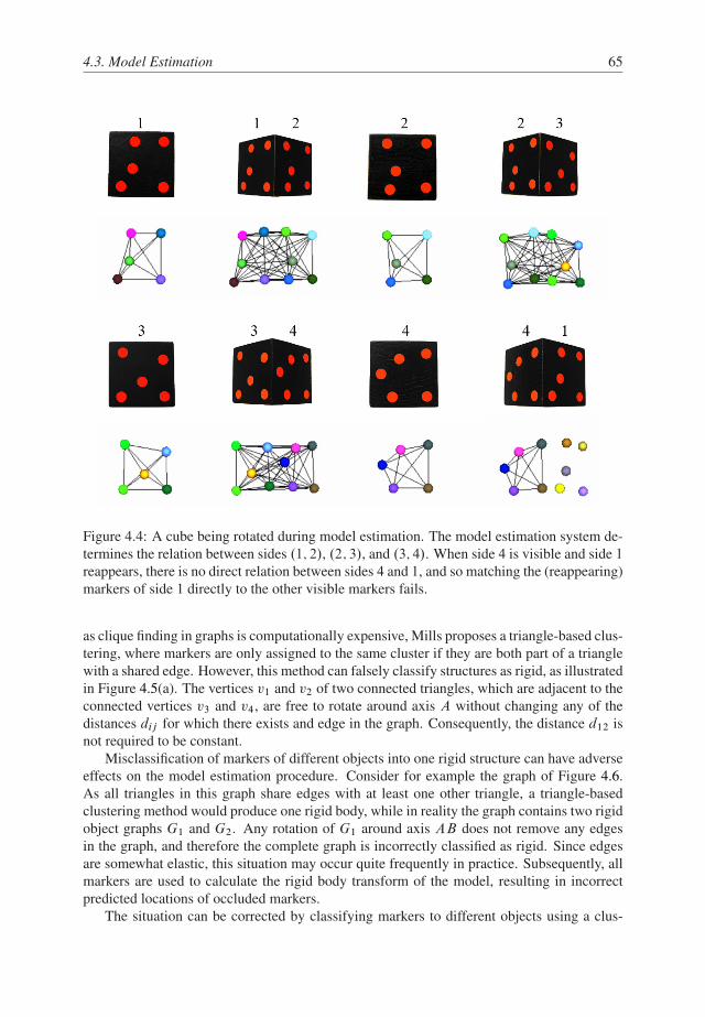
4.3. Model Estimation 65
Figure 4.4: A cube being rotated during model estimation. The model estimation system de-
termines the relation between sides .1; 2/, .2; 3/, and .3; 4/. When side 4 is visible and side 1
reappears, there is no direct relation between sides 4 and 1, and so matching the (reappearing)
markers of side 1 directly to the other visible markers fails.
as clique finding in graphs is computationally expensive, Mills proposes a triangle-based clus-
tering, where markers are only assigned to the same cluster if they are both part of a triangle
with a shared edge. However, this method can falsely classify structures as rigid, as illustrated
in Figure 4.5(a). The vertices v1 and v2 of two connected triangles, which are adjacent to the
connected vertices v3 and v4, are free to rotate around axis A without changing any of the
distances dij for which there exists and edge in the graph. Consequently, the distance d12 is
not required to be constant.
Misclassification of markers of different objects into one rigid structure can have adverse
effects on the model estimation procedure. Consider for example the graph of Figure 4.6.
As all triangles in this graph share edges with at least one other triangle, a triangle-based
clustering method would produce one rigid body, while in reality the graph contains two rigid
object graphs G1 and G2. Any rotation of G1 around axis AB does not remove any edges
in the graph, and therefore the complete graph is incorrectly classified as rigid. Since edges
are somewhat elastic, this situation may occur quite frequently in practice. Subsequently, all
markers are used to calculate the rigid body transform of the model, resulting in incorrect
predicted locations of occluded markers.
The situation can be corrected by classifying markers to different objects using a clus-
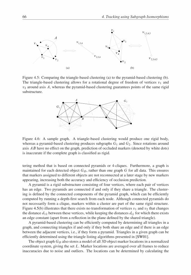
66 4. Tracking using Subgraph Isomorphisms
(a) (b)
Figure 4.5: Comparing the triangle-based clustering (a) to the pyramid-based clustering (b).
The triangle-based clustering allows for a rotational degree of freedom of vertices v1 and
v2 around axis A, whereas the pyramid-based clustering guarantees points of the same rigid
substructure.
Figure 4.6: A sample graph. A triangle-based clustering would produce one rigid body,
whereas a pyramid-based clustering produces subgraphs G1 and G2. Since rotations around
axis AB have no effect on the graph, prediction of occluded markers (denoted by white dots)
is inaccurate if the complete graph is classified as rigid.
tering method that is based on connected pyramids or 4-cliques. Furthermore, a graph is
maintained for each detected object GO , rather than one graph G for all data. This ensures
that markers assigned to different objects are not reconnected at a later stage by new markers
appearing, increasing both the accuracy and efficiency of occlusion prediction.
A pyramid is a rigid substructure consisting of four vertices, where each pair of vertices
has an edge. Two pyramids are connected if and only if they share a triangle. The cluster-
ing is defined by the connected components of the pyramid graph, which can be efficiently
computed by running a depth-first search from each node. Although connected pyramids do
not necessarily form a clique, markers within a cluster are part of the same rigid structure.
Figure 4.5(b) illustrates that there exists no transformation of vertices v1 and v2 that changes
the distance d12 between these vertices, while keeping the distances dij for which there exists
an edge constant (apart from a reflection in the plane defined by the shared triangle).
A pyramid-based clustering can be efficiently computed by determining all triangles in a
graph, and connecting triangles if and only if they both share an edge and if there is an edge
between the adjacent vertices, i.e., if they form a pyramid. Triangles in a given graph can be
efficiently determined using the triangle listing algorithms presented in [SW01].
The object graph GO also stores a model of all 3D object marker locations in a normalized
coordinate system, giving the set L. Marker locations are averaged over all frames to reduce
inaccuracies due to noise and outliers. The locations can be determined by calculating the

4.3. Model Estimation 67
rigid body transform that maps the identified markers to the corresponding model markers in
a least-squares manner [Hor87]. This transform is used to predict the locations of occluded
markers. When a marker is found for which no frame-to-frame correspondence could be
established, its location is compared to the predicted occluded marker locations. If the error
of the rigid body transform is too large, a combination of the given points is used to obtain a
new transform. This procedure is repeated until all combinations are tried, or a combination
is found that results in an accurate rigid body transform.
4.3.4 Model Estimation Summary
Given the 2D blob locations, the following steps are performed:
1. Marker tracking
The 3D locations of the 2D blobs detected in the camera images are determined us-
ing stereo correspondence, as described in Section 4.2. Markers are associated with
the markers in the previous frame by frame-to-frame correspondence, such that each
marker has a unique ID that stays constant during the time it is visible.
2. Edge updating
For each object graph GO , the edges between visible markers within the model are
updated. If the distance between two visible markers remains constant, the average
distance is updated. Otherwise, the edge is removed.
3. Invalid marker removal
In certain circumstances, the blob detector may find blobs that do not correspond to
valid markers. For instance, these blobs may come from objects in the workspace that
reflect incoming infrared lighting. If these undesired blobs are present in multiple cam-
era images, this may result in false 3D marker positions. However, these markers are
usually only visible for a short period of time or are located far from the input device.
These markers are therefore easily detected and removed from the object graphs by
checking their age and by using distance-based clustering techniques.
4. Graph clustering
Each object graph GO is split into new object graphs if necessary, by performing the
pyramid-based graph clustering technique.
5. Occluded marker prediction
The rigid body transform of each object is calculated and the locations of its occluded
markers are predicted. Next, all markers for which no frame-to-frame correspondence
could be established are compared to these occluded markers, and if they are close
enough to each other, the marker is recognized as a reappearing marker. Its ID and
age are updated with those of the occluded marker. Note that only markers that are
considered reliable are used to compute the rigid body transform.
6. New marker insertion
New markers that have not been recognized as reappearing markers are inserted into
all object graphs.

68 4. Tracking using Subgraph Isomorphisms
4.4 Model-based Object Tracking
The input to the tracking system is an estimated model graph Gm D .V; L; E/ as defined
in Section 4.3.1. The tracking system needs to identify a subset of this graph in the image
points. This is closely related to the double subgraph isomorphism problem. A subgraph G1
is isomorphic to another subgraph G2 if there is a one-to-one correspondence between their
vertices and there is an edge between two vertices of G1 if and only if there is an edge between
the corresponding vertices in G2. As this problem is known to be NP -complete [AF98], the
problem is simplified by defining a minimum size Smin of a subgraph of Gm which needs to
be present in a data graph Gd , with the constraint that this subgraph is a clique. Parameter
Smin defines how many markers are needed to unambiguously identify a model graph, and
each set of Smin markers that can be visible simultaneously is by definition fully connected.
Note that Smin can be determined during model estimation.
Tracking Method
The first step is to preprocess the model graph Gm. A hash table is constructed which indexes
each distance between vertices vi and vj for which there exists an edge eij . The table stores
pointers back to the model and the vertices vi and vj . The tracking method proceeds as
follows.
� A data point p is chosen, and the distance d D jjp�pj jj between p and all other data
points pj is indexed into the hash table.
� Each vertex vk in Gm maintains a list of possible matching data and model point pairs
.pj ; vl /. Therefore, a set of candidates is created for each vk , for which jjp � pj jj Djjvk � vl jj.
� If p matches vk , there must be a combination of matches between data points pj and
model points vl which is fully connected and for which the remaining distances are
correct, since by definition each set of Smin matching points must form a clique. As
such, each combination of three points of each candidate is checked for the remaining
distances with the model. If these match, a subgraph isomorphism of size four has been
found.
� The rigid body transform matching the model to the data graph is found by least-
squares [Hor87].
� All data points are transformed to the model coordinate system, and compared to the
model points. If at least Smin matching points are found, the tracking system can
mark the model as identified and stop the search for this model. However, to increase
robustness, all candidates are examined and the one that matches the image points best
is selected. This best fit is found by minimizing the sum of distances between model
and transformed data points defined by
F D 1
N
NX
iD1
jjpj � OMdevvi jj (4.11)
where OMdev is the transform that maps the model points to the data points, vi denotes
a recognized model point, and pj is its corresponding data point.

4.4. Model-based Object Tracking 69
Figure 4.7: (Left) An example model graph Gm with vertices vi and distances a; : : : ; i .
(Right) A data graph Gd with points pi , which has a double subgraph isomorphism with
Gm
� Chapter 5 includes a mathematical analysis on the influence of the number of features
used during pose estimation on accuracy. Since accuracy is shown to be a function
of the number of features, the pose estimation is refined using the downhill simplex
method as discussed in Section 3.3.3, which uses all detected data points. The function
to be minimized is the sum of minimum distances between the N matching data points,
transformed to the model coordinate system, and the corresponding model points.
Note that the tracking method implicitly exploits the fact that an edge is only present if the
two markers can be simultaneously visible, thus greatly reducing the number of candidates.
Optimizations
The tracking procedure can exploit frame-to-frame correspondence in order to speed up the
matching process. When the tracking system has identified an interaction device at a certain
time t , and frame-to-frame correspondence results in enough identified points at time t C�t
that correspond to points at time t , the pose of the device is directly derived from these
points. In this case, the complete search procedure is skipped. In case frame-to-frame cor-
respondence results in only one or two identified points, these points can be used as starting
points for the search.
Tracking Example
As an example of the tracking procedure, consider the model and data graphs of Figure 4.7.
This situation could occur when model point v5 is occluded, v2 and v5 cannot be visible
simultaneously, and data points p3 and p4 represent spurious markers.
The method first determines the distance matrix of the data graph Gd and the hash table H of
the model. The distance matrix of the data graph Gd is given by
Md D
0
B
B
B
B
B
B
@
0 a s 0 f b
a 0 d 0 b e
s d 0 v 0 t
0 0 v 0 0 u
f b 0 0 0 c
b e t u c 0
1
C
C
C
C
C
C
A
The hash table H of Gm, omitting model pointers, is given by
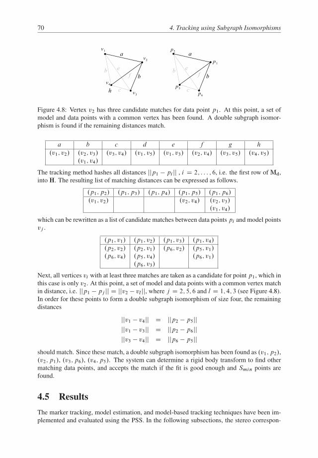
70 4. Tracking using Subgraph Isomorphisms
Figure 4.8: Vertex v2 has three candidate matches for data point p1. At this point, a set of
model and data points with a common vertex has been found. A double subgraph isomor-
phism is found if the remaining distances match.
a b c d e f g h
.v1; v2/ .v2; v3/ .v3; v4/ .v1; v5/ .v1; v3/ .v2; v4/ .v3; v5/ .v4; v5/
.v1; v4/
The tracking method hashes all distances jjp1 � pi jj , i D 2; : : : ; 6, i.e. the first row of Md,
into H. The resulting list of matching distances can be expressed as follows.
.p1; p2/ .p1; p3/ .p1; p4/ .p1; p5/ .p1; p6/
.v1; v2/ .v2; v4/ .v2; v3/
.v1; v4/
which can be rewritten as a list of candidate matches between data points pi and model points
vj .
.p1; v1/ .p1; v2/ .p1; v3/ .p1; v4/
.p2; v2/ .p2; v1/ .p6; v2/ .p5; v1/
.p6; v4/ .p5; v4/ .p6; v1/
.p6; v3/
Next, all vertices vi with at least three matches are taken as a candidate for point p1, which in
this case is only v2. At this point, a set of model and data points with a common vertex match
in distance, i.e. jjp1 � pj jj D jjv2 � vl jj, where j D 2; 5; 6 and l D 1; 4; 3 (see Figure 4.8).
In order for these points to form a double subgraph isomorphism of size four, the remaining
distances
jjv1 � v4jj D jjp2 � p5jjjjv1 � v3jj D jjp2 � p6jjjjv3 � v4jj D jjp6 � p5jj
should match. Since these match, a double subgraph isomorphism has been found as .v1; p2/,
.v2; p1/, .v3; p6/, .v4; p5/. The system can determine a rigid body transform to find other
matching data points, and accepts the match if the fit is good enough and Smin points are
found.
4.5 Results
The marker tracking, model estimation, and model-based tracking techniques have been im-
plemented and evaluated using the PSS. In the following subsections, the stereo correspon-

4.5. Results 71
dence method is compared to an approach using only the epipolar constraint, and the robust-
ness and performance of the model estimation and tracking methods are evaluated.
4.5.1 Stereo Correspondence
A straightforward method for stereo correspondence is to match all pairs of points in two
camera images that are within a certain epipolar distance of each other. However, this
method generates many false matches when multiple points are close to the same epipolar
line. Figure 4.9 illustrates the difference between this approach and the SVD-based matching
approach. Figure 4.9(a) shows three objects in the tracking volume, from a point of view
(a) (b)
(c) (d)
Figure 4.9: Stereo correspondence. (a) Three devices in the workspace. (b) The corre-
sponding camera images. (c) Resulting 3D marker locations of stereo matching by epipolar
constraint only. (d) Resulting 3D marker locations of the SVD-based stereo correspondence.

72 4. Tracking using Subgraph Isomorphisms
(a) (b)
(c) (d)
Figure 4.10: Four frames during simultaneous model estimation of the cubical and spherical
objects of Figure 4.2. The colored spheres represent the visible markers of the model, where
the colors encode the unique marker identifiers. (a) Initially, all points are regarded as one
object. (b) After some movement, edges are removed and the system correctly identifies two
objects. (c) During model estimation, occluded point locations are predicted and drawn with
grey cubes. (d) The system correctly modeled the two objects.
from the cameras. Figure 4.9(b) shows the blobs in the corresponding camera images, while
Figures 4.9(c) and (d) depict the output of stereo correspondence by epipolar matching, and
stereo correspondence by SVD matching, respectively. The SVD-based correspondence suc-
cessfully identifies the correct 3D marker locations, whereas the epipolar matching generates
too many additional false matches for reliable model estimation.
4.5.2 Model Estimation
Figure 4.10 depicts three frames of a data sequence of 2200 frames (36 seconds), where a
spherical object of diameter 7 cm and a cubical object of 7�7�7 cm are trained simultane-
ously (see Figure 4.2). These objects are equipped with 24 and 30 markers, respectively. The
figure shows that initially, all points are regarded as a single object. In the second frame,
after some movement, connections between new points and previously identified points are
created, and connections between points not rigidly attached are removed. At this point, the
model estimation system correctly identified two objects. Note that a triangle-based cluster-
ing of this graph would result in only one object. In the last frame, after a data sequence
of only 36 seconds, the system correctly identified two objects and created a model of all
markers attached to the objects. Creating these models by hand is obviously a very difficult
and time consuming task.
Figure 4.11 gives the total computation time the model estimation procedure requires for

4.5. Results 73
0
2
4
6
8
10
0 500 1000 1500 2000
tim
e (
ms)
frame
Figure 4.11: Computational time of simultaneous model estimation of a spherical and cubical
object of 30 and 24 markers.
each frame for the same data sequence as Figure 4.10, excluding image grabbing and blob
detection. Frame rates were measured using a system with a 2.2 GHz Pentium IV CPU and
1 Gb RAM. The computation time slowly increases while the objects are being moved, as
more points appear and the models get more complex. Most of the time is spent in the graph
clustering procedure (less than 1 ms is spent on stereo correspondence). The figure shows
that the time required to update the models is well below 10 ms. This implies that two objects
with a total of 54 markers can be trained with a frame rate of 60 Hz, which is limited by the
speed of the cameras. Therefore, the model estimation system provides instant feedback to
the developer of the acquired object model, such that model estimation errors are detected at
an early stage, and feedback is given about model completion.
4.5.3 Tracking
The performance of the tracking method presented in this chapter is compared with a pattern-
based tracker based on matching distances, as described in [LR04] (see Chapter 2 for more
details). The tracking method based on finding subgraph isomorphisms is referred to as
the subgraph tracker. Two wooden cubes of sizes 7�7�7 cm and 5�5�5 cm were used as
interaction devices. For each cube, 6 patterns of 5 points were defined for the pattern tracker,
and the object was trained for the subgraph tracker. Next, a data set was recorded, where both
cubes were manipulated simultaneously with both slow motions, and faster, more erratic
movements. For both trackers, the computational time required by the tracking method was
examined, excluding image grabbing and blob detection. Blob detection takes approximately
8 ms on average. Both trackers examine all candidate matches, and select the one with the
lowest distance metric as defined by Equation 4.11. This results in comparable accuracy of
both trackers.
The miss and hit rates of both tracking method were determined for an object exploration
task using two input devices, i.e., the number of frames the cubes could not be found (misses)
versus the number of frames the cubes were identified (hits). Table 4.1 shows the performance
of both trackers in terms of hits and misses. The table indicates that the pattern-based tracker
does not handle partial occlusion as well as the subgraph tracker. This can be attributed to
the fact that the pattern-based tracker does not deal with multiple partially visible patterns,
while in these situations the subgraph tracker has enough information to correctly identify the
device and its pose. Both trackers perform well for the noise levels introduced by the optical
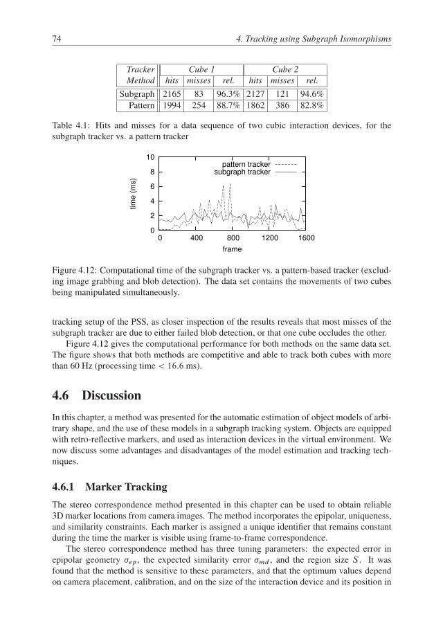
74 4. Tracking using Subgraph Isomorphisms
Tracker Cube 1 Cube 2
Method hits misses rel. hits misses rel.
Subgraph 2165 83 96.3% 2127 121 94.6%
Pattern 1994 254 88.7% 1862 386 82.8%
Table 4.1: Hits and misses for a data sequence of two cubic interaction devices, for the
subgraph tracker vs. a pattern tracker
0
2
4
6
8
10
0 400 800 1200 1600
tim
e (
ms)
frame
pattern trackersubgraph tracker
Figure 4.12: Computational time of the subgraph tracker vs. a pattern-based tracker (exclud-
ing image grabbing and blob detection). The data set contains the movements of two cubes
being manipulated simultaneously.
tracking setup of the PSS, as closer inspection of the results reveals that most misses of the
subgraph tracker are due to either failed blob detection, or that one cube occludes the other.
Figure 4.12 gives the computational performance for both methods on the same data set.
The figure shows that both methods are competitive and able to track both cubes with more
than 60 Hz (processing time < 16:6 ms).
4.6 Discussion
In this chapter, a method was presented for the automatic estimation of object models of arbi-
trary shape, and the use of these models in a subgraph tracking system. Objects are equipped
with retro-reflective markers, and used as interaction devices in the virtual environment. We
now discuss some advantages and disadvantages of the model estimation and tracking tech-
niques.
4.6.1 Marker Tracking
The stereo correspondence method presented in this chapter can be used to obtain reliable
3D marker locations from camera images. The method incorporates the epipolar, uniqueness,
and similarity constraints. Each marker is assigned a unique identifier that remains constant
during the time the marker is visible using frame-to-frame correspondence.
The stereo correspondence method has three tuning parameters: the expected error in
epipolar geometry �ep , the expected similarity error �md , and the region size S . It was
found that the method is sensitive to these parameters, and that the optimum values depend
on camera placement, calibration, and on the size of the interaction device and its position in
4.6. Discussion 75
the workspace. To further increase the robustness of the stereo correspondence method, these
parameters could be estimated adaptively.
4.6.2 Model Estimation
The model estimation method can handle virtually any shape, as long as at least three non-
collinear points are visible and recognized, in order to establish a relation with new points.
Short-term occlusion is handled by predicting the location of occluded markers. The method
can estimate multiple object models with a moderate amount of markers simultaneously.
Since objects that are identified as separate clusters are never reconnected, the graph cluster-
ing method never needs to handle more points than are on a device, making the complexity
practically linear in the number of devices. The worst case performance of the clustering
method occurs when the graph is fully connected. A fully connected graph has�
N3
�
D O.N 3/
triangles, where each triangle forms a pyramid with 3.N � 3/=2 other triangles. Therefore,
the worst case computational complexity is O.N 4/, which could be improved by updating
the pyramid graph incrementally. In practice, three objects of 30 markers can be trained with
high frame rates.
The model estimation method assumes that motions are slow and smooth, and that the 3D
data is reasonably reliable. This means that mistakes in marker tracking or blob detection (e.g.
multiple blobs that become one when they are aligned during rotation), may result in model
errors. In order to support faster and more erratic motions, the following strategies can be
applied. First, a predictive filtering technique can be used to estimate 3D marker locations,
so that outliers and jittering can be reduced. The filter can also be used to predict marker
locations more accurately, resulting in more reliable frame-to-frame correspondence. Second,
the robustness of the blob detection can be increased by incorporating marker quality metrics.
For instance, the roundness of a blob can be checked, so that two markers forming one blob in
a camera image can be rejected. Third, in case frame-to-frame correspondence is completely
lost, the tracking method can be applied using the model acquired so far, until a known
part of the model is found again. This occurs when less than three non-collinear markers
remain visible. This would also enable a developer to completely remove an object from the
workspace during model estimation, and insert it at a later time, or even to completely stop
the model estimation procedure to resume it at a later time.
4.6.3 Model-based Tracking
The tracking method treats the markers on an interaction device as one point-cloud, and
does not require markers to be grouped into patterns. This makes the system more flexible
compared to pattern-based approaches. For instance, in the situation illustrated in Figure 4.13,
two sides of a cube are partially occluded. The pattern-based approach using points would fail
to recognize the object even though seven markers are visible, whereas the subgraph tracker
correctly identifies the cube and its pose.
Results show the method is competitive with a pattern-based approach in terms of com-
putational efficiency, and more robust against occlusion. Although it would be possible to
use a pattern-based tracker with a trained device model by generating all patterns from the
model, this would require a prohibitive amount of patterns. For instance, an object with 30
markers would require�
305
�
D 142506 patterns. Although this number can be decreased by
using visibility information, the number of patterns required is clearly too large for realtime
tracking.

76 4. Tracking using Subgraph Isomorphisms
Figure 4.13: A partially occluded cube. A pattern-based tracking approach would fail to
recognize the object, as the two visible sides are partially occluded by the user’s hand. The
subgraph tracker correctly identifies the object and determines its pose.
There is a tradeoff between tracking speed and the allowed noise levels in marker distance.
Higher noise levels mean that more distances are indexed into the same location in the hash
table, and generate more candidates. In the implemented tracking system, noise levels were
set so that the distance error could not exceed 4 mm. In this case, two objects of each 30
markers can be tracked with over 60 Hz. With a much larger number of markers, performance
degrades.
The accuracy of the tracking method is identical to pattern-based approaches that opti-
mize the pose estimate by performing a fit on all data, minimizing Equation 4.11. Accuracy
depends on the size of the object, where a smaller object results in more jitter in the pose,
and on the quality of the blob detection, which is related to the distance of the object to the
cameras and lighting conditions.
4.7 Conclusion
In this chapter, an optical tracking system has been presented, which is capable of automatic
model estimation and tracking of objects of arbitrary shape. The system is marker-based,
allowing a developer to equip an object with retro-reflective markers, and train the system to
recognize the object by moving it in front of the cameras. The tracking method is based on
subgraph matching, finding a subset of the model graph in the data.
Results show that the system is robust against partial occlusion, noise, and outliers in the
data, and maintains frame rates of 60 Hz while performing model estimation or tracking of
two objects of 30 markers simultaneously.
The system can be extended to support fast and erratic motions during model estima-
tion. This can be achieved by incorporating the tracking method into the model estimation
procedure in case of loss of frame-to-frame correspondence.

Chapter 5
Analysis of Tracking Methods
In Chapters 3 and 4, two optical tracking methods were proposed for pose estimation of input
devices. The approaches are based on different principles: one performs object recognition
completely in 2D, whereas the other transforms detected image features to 3D and performs
3D subgraph matching for recognition. Each method was compared to a related tracking
approach.
The goal of this chapter is to analyze the behavior of tracking methods that are based
on different principles, subject to the error sources as defined in Chapter 2. Three tracking
methods are selected: the method based on projection invariant properties as presented in
Chapter 3; the method based on finding subgraph isomorphisms in 3D as presented in Chap-
ter 4; and a method based on pose estimation by optimization as discussed in Section 2.5.3.
This chapter presents an experimental evaluation of these tracking methods to study the
effects of each error source on the accuracy, latency, and robustness of each method. Fur-
thermore, an error model for accuracy is presented, which is used to analyze the influence
of the different error sources, and compared to experimentally obtained data. Results show
that each of the tracking methods has its own advantages and disadvantages, and that none of
the tested methods is robust to every error source. Furthermore, the accuracy model is shown
to result in reasonable predictions of the accuracy of the tracking methods for a given error
source value.
The chapter is organized as follows. In Section 5.1, the evaluation method is described.
Next, the test setup and performance metrics are discussed. Section 5.2 provides an accuracy
model of optical tracking methods, subject to different error sources. In Section 5.3, the
results are presented. Section 5.4 provides a discussion of the results. Finally, in Section 5.5
conclusions are given.
5.1 Method
The fundamental problem in model-based optical tracking is to match the data features ob-
tained from camera images to a device model, and to obtain a pose estimate of each in-
teraction device. As discussed in Chapter 2, optical tracking methods can be divided into
categories based on how recognition and pose estimation is performed.
In this chapter, three tracking solutions are compared that are based on different principles:
� The pencil tracker
The pencil tracker, as presented in Chapter 3, is based on 2D recognition using projec-
tion invariant properties of line pencils. The approach outperforms a related approach
based on point features with respect to occlusion and efficiency.
77

78 5. Analysis of Tracking Methods
(a) (b)
Figure 5.1: Cubic devices with (a) point patterns and (b) line pencils.
� The subgraph tracker
The subgraph tracker is presented in Chapter 4. It uses stereo correspondence to trans-
form 2D image points to 3D, and uses a 3D recognition method based on subgraph
isomorphisms for point identification. It is demonstrated in Chapter 4 that this method
outperforms a related pattern-based approach with respect to occlusion and generic
device shape.
� The iterative closest point (ICP) tracker
The ICP tracker, as discussed in Section 2.5.3, is based on projecting the model points
of a device back into the camera images, given a device pose. A fitting procedure is
performed to refine the pose, matching the projected device features to the 2D image
features.
The performance of the tracking methods is experimentally compared, subject to the fol-
lowing error sources (see Chapter 2): lighting conditions, the amount of occlusion, and the
camera parameters determined by calibration.
5.1.1 Test Setup
Environment
For the experimental evaluation of tracking methods, simple wooden cubes were used as input
devices. For the subgraph and ICP trackers, which use point features, retro-reflective markers
were attached to a cube, and a model was trained using the model estimation techniques
presented in Chapter 4. For the pencil tracker, a cube was equipped with six pencils, one for
each side of the cube. A model of this cube was obtained by training the pencils using the
techniques presented in Chapter 3, and by measuring the location of each pencil on the device
by hand. Figure 5.1 shows the devices used in this study.
The experiments were conducted in the PSS. The tracking setup is discussed in Sec-
tion 2.6. The experiments were performed on an AMD Athlon XP 2700+ with 1 Gb RAM.

5.1. Method 79
Z
X
Y
Z
(a)
Z
X
Y
Z
(b)
Figure 5.2: The 3D data recordings in the xy, xz, and yz planes. Depicted are (a) the
recordings in the interaction volume, and (b) the 2D projections of each recording onto its
corresponding plane.
Data Set Generation
To compare different tracking methods with respect to accuracy, a data set is required. The
data set was created by recording an interactive session of a user exploring a virtual object
using the tracking system, and storing the pose of the interaction device on disk. This se-
quence of poses provides a “ground truth”, which is used to determine the performance of
each of the tracking methods. Figure 5.2 shows the trajectories of the device frames during
the interactive session. The recorded data set consists of 700 frames.
The data set is used to generate synthetic camera images for the tracking methods. The
camera images are generated such that the effect of occlusion on each tracking method can
be determined. Occlusion is added by blocking out certain regions in the camera images.
The pinhole camera model as discussed in Chapter 2 is used to project the 3D model
features back to the camera images, given a pose in the data set. This process generates the
ideal images: no image distortion or image noise is added, and all error sources are zero. By
varying the error sources defined in Section 2.7, the accuracy of the tracking methods can be
compared.
The images were generated by using OpenGL drawing routines. The device model used
by the subgraph and ICP trackers, which describes the 3D marker locations on the input
device, was used to draw white blobs with a diameter of 4.2 pixels with subpixel accuracy.
Similarly, the model used by the pencil tracker, which describes the 3D line pencils on the
input device, was used to draw white lines with a thickness of 3 pixels and a 3D length of 7
cm. These values correspond to the actual imagery obtained by the cameras.
Parameter Perturbation
The error sources were varied as follows:
� Lighting conditions
To simulate changing lighting conditions, the data set was projected using the ideal
camera parameters, and adding zero mean Gaussian noise with variance �2p D 0:2 and
�2p D 0:5 pixels2 to the coordinates of each 2D data feature. For the subgraph and ICP
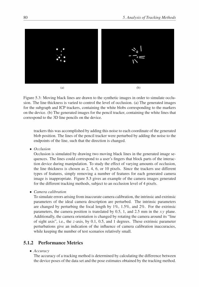
80 5. Analysis of Tracking Methods
(a) (b)
Figure 5.3: Moving black lines are drawn to the synthetic images in order to simulate occlu-
sion. The line thickness is varied to control the level of occlusion. (a) The generated images
for the subgraph and ICP trackers, containing the white blobs corresponding to the markers
on the device. (b) The generated images for the pencil tracker, containing the white lines that
correspond to the 3D line pencils on the device.
trackers this was accomplished by adding this noise to each coordinate of the generated
blob position. The lines of the pencil tracker were perturbed by adding the noise to the
endpoints of the line, such that the direction is changed.
� Occlusion
Occlusion is simulated by drawing two moving black lines in the generated image se-
quences. The lines could correspond to a user’s fingers that block parts of the interac-
tion device during manipulation. To study the effect of varying amounts of occlusion,
the line thickness is chosen as 2, 4, 6, or 10 pixels. Since the trackers use different
types of features, simply removing a number of features for each generated camera
image is inappropriate. Figure 5.3 gives an example of the camera images generated
for the different tracking methods, subject to an occlusion level of 4 pixels.
� Camera calibration
To simulate errors arising from inaccurate camera calibration, the intrinsic and extrinsic
parameters of the ideal camera description are perturbed. The intrinsic parameters
are changed by perturbing the focal length by 1%, 1.5%, and 2%. For the extrinsic
parameters, the camera position is translated by 0.5, 1, and 2.5 mm in the xy plane.
Additionally, the camera orientation is changed by rotating the camera around its “line
of sight axis”, i.e., the z-axis, by 0.1, 0.5, and 1 degrees. These extrinsic parameter
perturbations give an indication of the influence of camera calibration inaccuracies,
while keeping the number of test scenarios relatively small.
5.1.2 Performance Metrics
� Accuracy
The accuracy of a tracking method is determined by calculating the difference between
the device poses of the data set and the pose estimates obtained by the tracking method.

5.2. Accuracy Model 81
The accuracy of a pose estimate is divided into the positional and angular accuracy.
The positional accuracy is defined as the root mean square error (RMSE) of the dif-
ference in position between the poses of the data set and the pose estimates from the
tracking method, as defined by
RMSEt D
v
u
u
t
1
N
NX
iD1
jjT refi � T est
i jj2 (5.1)
where N is the number of frames in the motion sequence, Trefi is the device position
of the data set, and T esti represents the estimated device position at frame i . Similarly,
the rotational accuracy is defined as the root mean square error of the difference in
orientation between the poses of the data set and the pose estimates
RMSEr D
v
u
u
t
1
N
NX
iD1
.360
�cos�1..qri
� q�1ei
/w//2 (5.2)
where qe is the quaternion representing the estimated orientation, qr represents the
reference signal, and qw represents the w-component of quaternion q.
� Latency
The latency of a tracking method is defined as the time required for image capturing,
feature detection, recognition, and pose estimation. In the tracking framework of Fig-
ure 2.2, this time is given by t2 � t1. Although this is not the complete end-to-end
latency of the system, it is a good and convenient metric to compare different tracking
methods.
� Robustness
The robustness of each method is determined by counting the number of frames in
which the tracking method fails to recognize the input device and estimate its pose.
This number of misses determines if a method is robust: if a device cannot be found
for a certain parameter perturbation, the method is not considered to be robust with
respect to this parameter. For instance, a method might fail due to partial occlusion or
small inaccuracies in the camera parameters. The number of misses gives an indication
of the sensitivity of a tracking method with respect to different error sources.
5.2 Accuracy Model
This section provides an error model of accuracy, which is used to analyze the influence of
the different error sources. This analysis is used to predict the accuracy of optical tracking
methods under different circumstances. The obtained data is compared to the experimentally
obtained data in Section 5.3.
5.2.1 Image Noise
To model image noise, a stereo camera setup is assumed, where point features are detected
in each camera image. Figure 5.4 illustrates a parallel stereo camera setup with cameras C1

82 5. Analysis of Tracking Methods
Figure 5.4: The expected error of a reconstructed 3D point P in a stereo camera setup, given
its noisy 2D image projections.
and C2, a focal length f , and an image plane E. A 3D point P with a depth d to the baseline
of the cameras is projected onto E. Assuming the errors in the 2D point projections follow
a Gaussian distribution with standard deviation �p , the reconstructed 3D point P lies within
the region illustrated in the figure (see also [CS00]).
Expected Single Point Reconstruction Error
The region S can be described by the expected error �xy in the xy-direction, and �z in the
z-direction. The expected error �xy follows directly from Figure 5.4 by similar triangles as
�xy
dD �psp
f(5.3)
�xy D d�psp
f(5.4)
where �p is the standard deviation of the Gaussian image noise in pixels, and sp represents
the pixel size in meters. Similarly, the expected error �z follows from similar triangles as
�xy
�z
DId
2
d C �z
(5.5)
where Id is the distance between the cameras. This equation can be simplified by substituting
Equation 5.4, which results in
�z D2d2�psp
Id f � 2d�psp
(5.6)
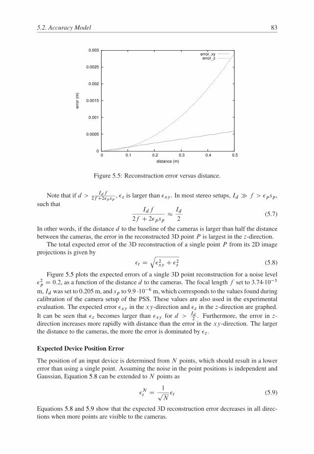
5.2. Accuracy Model 83
0
0.0005
0.001
0.0015
0.002
0.0025
0.003
0 0.1 0.2 0.3 0.4 0.5
err
or
(m)
distance (m)
error_xyerror_z
Figure 5.5: Reconstruction error versus distance.
Note that if d > Id f2f C2�psp
, �z is larger than �xy . In most stereo setups, Id � f > �psp ,
such thatId f
2f C 2�psp
� Id
2(5.7)
In other words, if the distance d to the baseline of the cameras is larger than half the distance
between the cameras, the error in the reconstructed 3D point P is largest in the z-direction.
The total expected error of the 3D reconstruction of a single point P from its 2D image
projections is given by
�t Dq
�2xy C �2
z (5.8)
Figure 5.5 plots the expected errors of a single 3D point reconstruction for a noise level
�2p D 0:2, as a function of the distance d to the cameras. The focal length f set to 3.74�10�3
m, Id was set to 0.205 m, and sp to 9.9 �10�6 m, which corresponds to the values found during
calibration of the camera setup of the PSS. These values are also used in the experimental
evaluation. The expected error �xy in the xy-direction and �z in the z-direction are graphed.
It can be seen that �z becomes larger than �xy for d > Id
2. Furthermore, the error in z-
direction increases more rapidly with distance than the error in the xy-direction. The larger
the distance to the cameras, the more the error is dominated by �z .
Expected Device Position Error
The position of an input device is determined from N points, which should result in a lower
error than using a single point. Assuming the noise in the point positions is independent and
Gaussian, Equation 5.8 can be extended to N points as
�Nt D
1pN
�t (5.9)
Equations 5.8 and 5.9 show that the expected 3D reconstruction error decreases in all direc-
tions when more points are visible to the cameras.

84 5. Analysis of Tracking Methods
Figure 5.6: The maximum orientation error.
Expected Device Orientation Error
The expected error in the estimated device orientation can be estimated as follows. Consider
a set of points Pi , which are shifted in relation to the device, for instance due to noise (see
Figure 5.6). Using the expected position error �t , the maximum orientation error can be
written as
� D 180
�p
Ntan�1 �t
0:5v(5.10)
where v represents the average distance from device points Pi to the center C of the device.
5.2.2 Camera Calibration Errors
Errors in the camera calibration are divided into two categories: errors in the intrinsic camera
parameters, and errors in the extrinsic camera parameters. In this study, errors in the intrinsic
camera parameters are modeled by focal length perturbations. The errors in the extrinsic
camera parameters are modeled by deviations in the camera position and orientation.
Focal Length
Errors in the focal length are modeled according to Figure 5.7. The figure depicts a stereo
setup with cameras C1 and C2. A 3D point P is projected onto the image plane E. The
cameras have a true focal length f . A deviation �f in the focal length causes the image
plane to be shifted, which shifts the location of the reconstructed 3D point to OP . The effect
is equivalent to the situation illustrated in Figure 5.7, where the camera positions are shifted
away from the image plane over a distance of �f . Similar triangles directly give the expected
error �f
�f C d C�f
Id
D �f C d � f
l(5.11)
�f D l.d C�f / � Id .d � f /
Id � l(5.12)

5.2. Accuracy Model 85
Figure 5.7: The expected error of a reconstructed 3D point P , given its 2D image projections
and an error in focal length.
where l represents the distance between the projected 2D image points.
Note that l can be written as a function of the depth of point P , the focal length, and the
distance between the cameras. The result is obtained from Figure 5.7 as
l D Id .d � f /
d(5.13)
Equation 5.12 gives the expected error of the reconstruction of a single point when the
focal length is inaccurate. When more than one point is used for determining the device
position, the exact expected error depends on the position and orientation of the device with
respect to the cameras. If N points lie in a plane parallel to the image plane E, the expected
error of the device position is equal to the expected error of a single point. Equation 5.12
serves as a maximum value of the reconstruction error.
Figure 5.8 illustrates how four points are transformed if the focal length is changed. The
3D reconstructed points are stretched in the z-direction. When multiple reconstructed 3D
points are used in an optimization procedure to match the reconstructed points to the device
model points, model points may be matched to incorrect reconstructed data points. This may
cause errors in both the device position and orientation.
Camera Position
The effects of errors in the camera position on the accuracy of the reconstructed 3D point
can be determined as follows. Consider a parallel stereo camera setup with cameras C1
and C2, as illustrated in Figure 5.9. A 3D point P with a depth d to the baseline of the
cameras is projected onto E. A positional error �C of camera C2 in the xy plane gives a 3D
reconstruction error of �cxyin the xy-direction and �cz
in the z-direction. Similar triangles

86 5. Analysis of Tracking Methods
Figure 5.8: The reconstruction of device points is stretched in the z-direction for changing
focal length.
Figure 5.9: The expected error of a reconstructed 3D point P , given its 2D image projections
and an error �C in camera position.

5.3. Results 87
Figure 5.10: The expected error of a reconstructed 3D point P , given its 2D image projections
and an error in camera orientation.
give the maximum reconstruction error:
�cxyD �C
2(5.14)
�czD d�C
Id
(5.15)
�c Dq
�2cxyC �2
cz(5.16)
Camera Orientation
A rotation of one of the cameras around the z-axis will result in an error in the reconstructed
3D point. The situation is depicted in Figure 5.10. A point P is projected onto the image
plane R of a camera C , resulting in the 2D projection p. Because of an error in the calibration
of the camera orientation, the 2D projected point is rotated around the z-axis to point Op. The
resulting error �pr in pixel position can be written as
�pr D 2rsin�
2(5.17)
The expected error �r in device position can be obtained by substituting the result of Equa-
tion 5.17 into Equation 5.8.
5.3 Results
The tracking methods were applied to the data set for each of the error sources. The following
sections present the results of the accuracy model and the experimental evaluation in terms
of the performance metrics as defined in Section 5.1.2.

88 5. Analysis of Tracking Methods
Image noise
0
0,5
1
1,5
2
2,5
3
SUB PEN ICP SUB PEN ICP
0.2 0.5
Tra
nsla
tio
na
l e
rro
r (m
m)
(a)
Image noise
0
0,5
1
1,5
2
2,5
3
3,5
4
4,5
SUB PEN ICP SUB PEN ICP
0.2 0.5
An
gu
lar
err
or
(de
g)
(b)
Figure 5.11: Translational and rotational errors for image noise levels of �2p D 0:2; 0:5. (a)
Translational errors in millimeters with 95% confidence intervals. (b) Rotational errors in
degrees with 95% confidence intervals.
5.3.1 Accuracy
Image Noise
It was found that the translational and rotational errors could be approximated well by a
Gaussian distribution. The t -distribution was used to determine 95% confidence intervals for
the average errors [DS98]. Figure 5.11 depicts the results for noise levels �2p D 0:2; 0:5.
Tables 5.1 and 5.2 list the translational and angular RMSE. The noise levels represent the
variance of the Gaussian noise added to the data set.
Table 5.1 also lists the expected translational error as obtained from Equation 5.9. The
parameters of the equation were obtained from the setup of the PSS. The distance d to the
cameras was determined to be approximately 0.5 m, the distance between the cameras Id
was 0.205 m, the focal length f of the cameras was 3.74�10�3 m, and the pixel size was 9.9
�10�6 m. The number of features N that were used in the pose estimation was determined to
be an average of five features for the subgraph and ICP trackers. The pencil tracker uses four
line features to determine the position of a pencil intersection and for pose estimation, and
therefore N was set to four in this case.
Table 5.2 includes the expected orientation error as determined by Equation 5.10. The
average distance v was set to 3.5 cm (the cube size is 7 cm). The values listed in Table 5.1
were used as noise levels �t in Equation 5.10.
The following observations can be made from Figure 5.11 and Tables 5.1 and 5.2:
� The pencil tracker is slightly less accurate than the subgraph and ICP trackers, although
the difference becomes statistically insignificant for �2p D 0:2 or 0:5. A possible cause
for accuracy differences is that the pencil tracker uses only four features per pattern
to determine a pose, whereas the subgraph and ICP trackers use a minimum of five
features.

5.3. Results 89
Subgraph Pencil ICP
Noise Measured Analytic Measured Analytic Measured Analytic
0.0 0.16 0.00 0.25 0.00 0.16 0.00
0.2 1.16 1.32 1.37 1.48 1.15 1.32
0.5 2.27 2.10 2.39 2.35 2.28 2.10
Table 5.1: Positional RMSE in millimeters, for image noise levels of �2p D 0:0; 0:2; 0:5.
Subgraph Pencil ICP
Noise Measured Analytic Measured Analytic Measured Analytic
0.0 0.24 0.00 0.33 0.00 0.27 0.00
0.2 1.79 1.89 1.92 2.24 1.73 1.89
0.5 3.48 3.69 3.82 3.89 3.48 3.69
Table 5.2: Angular RMSE in degrees, for image noise levels of �2p D 0:0; 0:2; 0:5.
The accuracy of the device pose computed with the subgraph tracker is very similar
to the one determined by the ICP tracker. This can be attributed to the nature of the
algorithms. Both trackers use all available data to determine the pose, and perform an
iterative optimization procedure to match the model points to the data points. The ICP
tracker projects the 3D device model points back to the 2D camera images, given a
device pose. It then iteratively refines this pose to fit the projected model points onto
the 2D data points. The subgraph tracker first transforms the 2D data points to 3D
space, and performs a similar iterative pose optimization procedure to match the 3D
model points to the 3D data points. Since both approaches use all available data, the
accuracy is very similar.
� The analytically determined values are reasonable estimations of the experimentally
obtained results. The standard deviation as obtained from Equation 5.9 is a minimum
value of the RMSE. However, in some cases the analytically determined values are
slightly lower than the measured values. This can be attributed to quantization errors
in the point and line detection methods that precede the recognition and pose estimation
stages. These quantization effects are apparent from the fact that if no noise is added
to the data set, i.e., �2p is set to zero, the measured position errors are not zero.
The size of the quantization errors can be estimated as follows. The RMSE of the sub-
graph tracker for �2p D 0 is 0.16 mm. Substituting this error back into Equations 5.9,
5.4, and 5.6, a single point detection error with a variance of approximately 0.00295
pixel is obtained. This illustrates how very small errors during point detection can have
significant effects on the accuracy of pose estimation.
A better error estimate can be obtained by correcting the results from Equation 5.9 with
the expected quantization error.
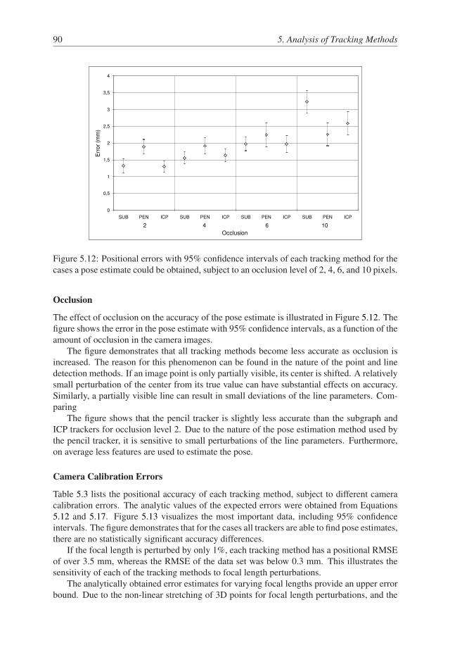
90 5. Analysis of Tracking Methods
Occlusion
0
0,5
1
1,5
2
2,5
3
3,5
4
SUB PEN ICP SUB PEN ICP SUB PEN ICP SUB PEN ICP
2 4 6 10
Err
or
(mm
)
Figure 5.12: Positional errors with 95% confidence intervals of each tracking method for the
cases a pose estimate could be obtained, subject to an occlusion level of 2, 4, 6, and 10 pixels.
Occlusion
The effect of occlusion on the accuracy of the pose estimate is illustrated in Figure 5.12. The
figure shows the error in the pose estimate with 95% confidence intervals, as a function of the
amount of occlusion in the camera images.
The figure demonstrates that all tracking methods become less accurate as occlusion is
increased. The reason for this phenomenon can be found in the nature of the point and line
detection methods. If an image point is only partially visible, its center is shifted. A relatively
small perturbation of the center from its true value can have substantial effects on accuracy.
Similarly, a partially visible line can result in small deviations of the line parameters. Com-
paring
The figure shows that the pencil tracker is slightly less accurate than the subgraph and
ICP trackers for occlusion level 2. Due to the nature of the pose estimation method used by
the pencil tracker, it is sensitive to small perturbations of the line parameters. Furthermore,
on average less features are used to estimate the pose.
Camera Calibration Errors
Table 5.3 lists the positional accuracy of each tracking method, subject to different camera
calibration errors. The analytic values of the expected errors were obtained from Equations
5.12 and 5.17. Figure 5.13 visualizes the most important data, including 95% confidence
intervals. The figure demonstrates that for the cases all trackers are able to find pose estimates,
there are no statistically significant accuracy differences.
If the focal length is perturbed by only 1%, each tracking method has a positional RMSE
of over 3.5 mm, whereas the RMSE of the data set was below 0.3 mm. This illustrates the
sensitivity of each of the tracking methods to focal length perturbations.
The analytically obtained error estimates for varying focal lengths provide an upper error
bound. Due to the non-linear stretching of 3D points for focal length perturbations, and the

5.3. Results 91
Parameter Accuracy
Type Value Subgraph Pencil ICP Analytic
intrinsic 1.0% 3.76 4.25 3.82 4.96
focal 1.5% 5.57 6.01 5.49 7.44
length 2.0% 6.12 7.76 - 9.93
extrinsic 0.5 0.97 1.08 0.95 1.24
camera 1.0 1.98 2.21 1.96 2.49
translation 2.5 5.23 5.49 5.24 6.22
extrinsic 0.1 0.23 0.39 0.23 0.23
camera 0.5 1.13 1.37 1.14 1.17
rotation 1.0 0.39 2.54 - 2.40
Table 5.3: Positional errors of each tracking method in millimeters, subject to perturbations
of intrinsic and extrinsic camera parameters.
Focal length perturbation
0
1
2
3
4
5
6
7
8
SUB PEN ICP SUB PEN ICP
1.0% 1.5%
Po
sitio
na
l e
rro
r (m
m)
(a)
Camera translation
0
1
2
3
4
5
6
7
SUB PEN ICP SUB PEN ICP
1.0 2.5
Po
sitio
na
l e
rro
r (m
m)
(b)
Figure 5.13: Positional errors with 95% confidence intervals of each tracking method for: (a)
Focal length perturbations of 1 and 1.5%. (b) Camera translation of 1 and 2.5 mm.

92 5. Analysis of Tracking Methods
0
20
40
60
80
100
120
140
0.0 0.2 0.5
Noise
Fra
mera
te (
fps)
Subgraph Pencil ICP
Figure 5.14: Average frame rates for each tracking method, subject to noise levels �2p D
0; 0:2; 0:5.
fact that each tracking method uses an optimization procedure to match the model features to
the data features, the values are lower in practice.
It was found that the ICP method is sensitive to camera calibration errors. Since the
method iteratively projects the model points back to 2D given a pose estimate and matches
these points to the data points, it relies on an accurate camera description. The table shows
that for a focal length perturbation of 2%, ICP is not able to determine a pose for all image
frames. Similarly, ICP fails to find a pose if the camera orientation is perturbed by one
degree. Although the subgraph and pencil trackers are able to find pose estimates under these
circumstances, large camera calibration errors result in inaccurate estimates.
5.3.2 Latency
Figure 5.14 depicts the average frame rate of each tracking method, subject to different noise
levels. The subgraph and pencil trackers are clearly faster than the ICP method. Also, it can
be seen that the performance of the subgraph and pencil trackers is not sensitive to noise,
whereas the ICP method becomes slower as noise increases. As more noise is added, the
likelihood of an occasional miss is increased. If the ICP tracker is not able to obtain a rea-
sonable initial pose estimate based on the pose of the previous frames, the method requires
many optimizations to find a good pose estimate near the global minimum.
Figure 5.15 plots the accumulative latency of each tracking method for the data set. The
slopes of the subgraph and pencil plots are practically constant. The slope of the ICP plot
often remains constant, but suffers from a number of large discontinuities. In these cases, the
initial pose estimate needed by the ICP method was not determined accurately enough.
In Chapter 1, the requirements for an optical tracking system were defined, with a mini-
mum frame rate of 60 Hz and a maximum latency of 33 ms. It is evident from the data that
the ICP method is in fact capable of reaching frame rates of around 60 Hz. However, the
discontinuities in the latency bring the average frame rate below the required 60 Hz, such that
the method is less suitable for real-time tracking.

5.3. Results 93
0
5
10
15
20
25
30
35
0 100 200 300 400 500 600 700
tim
e (
s)
frame
subgraphpencil
icp
Figure 5.15: Accumulative time for the tracking methods for the data set.
5.3.3 Robustness
Table 5.4 tabulates the robustness of each method, subject to different image noise levels,
occlusion, and camera parameter perturbations. The following observations can be made:
� Image noise
The ICP tracker is more robust against image noise than the subgraph and pencil track-
ers. The subgraph tracker uses stereo correspondence, which relies on epipolar geom-
etry. Errors in the epipolar geometry result in noisy 3D data points, resulting in a noisy
pose estimate. If the noise becomes larger, the epipolar distance between an image
point from one camera and a point in the other camera may exceed a certain threshold.
In this case, the two image points are not considered as possible matches, and the 3D
point cannot be determined correctly.
The pencil tracker uses the detected lines in a camera image to detect an interaction
device directly in 2D. Although image noise influences the cross ratio, the intervals in
which the cross ratios may lie are chosen relatively large (the range was set to 0.08).
As such, image noise has less influence on the device recognition, although larger cross
ratio intervals result in a smaller number of distinguishable pencils.
The ICP tracker uses a prediction of the device pose as an initial estimate, and itera-
tively refines this pose by projecting the model points to 2D and fitting these to the data
points. As such, noisy data points have less influence on the ICP method.
� Occlusion
The subgraph tracker suffers most from occlusion. Although in Chapter 4 the method
was shown to be more robust than a related tracking method using 3D pattern recog-
nition, the ICP and pencil trackers perform significantly better when features become
occluded. The reason is that the subgraph tracker requires points to be visible in two
cameras simultaneously in order to transform the point to 3D.
On the other hand, the ICP method can handle situations where different device points

94 5. Analysis of Tracking Methods
Parameter Misses
Type Value Subgraph Pencil ICP
Image 0.0 0 0 3
noise 0.2 10 3 4
0.5 253 143 56
occlusion 2 121 12 78
6 249 28 101
10 386 100 298
focal 1% 0 0 3
length 2% 208 0 700
camera 0.5 0 0 3
translation 2.5 53 0 189
camera 0.1 0 0 3
rotation 1.0 670 0 700
Table 5.4: The number of misses of each tracking method in a motion sequence of 700 frames
for varying noise levels, occlusion, and intrinsic and extrinsic camera parameters.
are visible in different cameras. As such, occlusion has less influence. However, the
computational requirements of the ICP method depend on the number of misses, mak-
ing the subgraph tracker preferable over ICP in practice.
The pencil tracker is the most robust against occlusion, due to the nature of the line
features. Since only an arbitrary point on the line and its direction is required for the
tracking method, only a small part of the line needs to be visible.
� Camera calibration
The ICP tracker strongly relies on an accurate description of the camera parameters.
If the focal length is miscalibrated by more than 1.5% of the reference focal length,
the method is unable to correctly determine the pose of the device. In this case, the
subgraph tracker is also not robust. If the camera translation is miscalibrated by 2.5
mm or more, or when the camera orientation is miscalibrated by 1 degree or more, the
subgraph and ICP trackers are not robust.
The pencil tracker is able to determine a device pose in all cases, and is the least sen-
sitive to calibration errors. Although miscalibrations have an effect on its accuracy, it
is the only method that is able to obtain a pose estimate in each of the tested camera
parameter perturbations.
5.4 Discussion
In the previous sections, three model-based optical tracking methods have been compared,
and their performance was evaluated analytically. The results are summarized by the three
performance criteria as defined in Section 5.1.2:
� Accuracy
The experimental data shows that the relative accuracy of the subgraph and ICP trackers
is better than the pencil tracker. A possible cause for this would be the number of

5.4. Discussion 95
features used during pose estimation. On average, the subgraph and ICP trackers use
more features to determine a pose estimate. The pose estimation procedure of the
pencil tracker could also be more sensitive to noise in the line directions. For instance,
it was observed that the pencil tracker is quite sensitive to the length of the generated
image lines.
The results show that the accuracy model developed in Section 5.2 gives a good indi-
cation of the worst case accuracy of the tracking methods, subject to image noise and
camera calibration errors.
Occlusion has a significant effect on the accuracy of each of the tracking methods. If
the level of occlusion is increased, the accuracy of the tracking methods decreases.
This can be attributed to the nature of the point and line detection methods. If a point
or line feature is partially occluded in the camera images, the center and line directions
can become distorted.
Focal length was demonstrated to have a large effect on the accuracy of each tracker,
increasing the positional RMSE of the subgraph tracker from its nominal value of 0.3
mm to more than 3.5 mm if the focal length is perturbed by just 1% of its reference
value. Perturbations in the extrinsic camera parameters were found to have a smaller
influence on accuracy.
� Latency
The data shows that the subgraph and pencil trackers have a lower latency than the ICP
tracker. The reason is that the ICP method is an optimization method that requires a
reasonable initial estimate of the solution. In cases where this initial estimate cannot be
obtained, or is not accurate enough, the procedure requires many optimizations to find
an estimate close to the global minimum. Figure 5.15 illustrates that the ICP tracker is
competitive with the other tracker if the initial estimate can be chosen near the global
minimum. However, ICP suffers from large performance penalties in case this initial
estimate cannot be determined accurately, for instance due to increased image noise,
occlusion or camera calibration errors.
The latency of a tracking method depends on the number of detected data features. The
computational complexity of a tracking method can be used to get an idea of how well
a method scales when the number of data features is increased.
The worst case computational complexity of the recognition step of the pencil tracker is
obtained when all lines in the camera image intersect at one point, resulting in�
N4
�
pen-
cils, where N is the number of detected line features. This results in a computational
complexity of O.N 4/.
The worst case computational complexity of the recognition step of the subgraph tracker
is obtained when all data and model points have the same distance, and the best match
is searched. In this case, the number of hashing collisions for a given data point is
O.N 2/, resulting in a candidate list of N data point matches for every model point.
Next, O.N 3/ distance checks need to be performed, resulting in a worst case complex-
ity of O.N 6/.
The worst case complexity of the ICP method depends on the method used as opti-
mization procedure. In this thesis, the downhill simplex method from Nelder and Mead
[Chv83] was used. Since no proof of convergence exists for this method, a complexity
analysis is not possible.

96 5. Analysis of Tracking Methods
Although the worst case computational complexity of the tracking methods are rela-
tively high, it was found that in practice the worst case computational complexities are
not reached. The pencil and subgraph trackers are capable of tracking two interaction
devices with each 30 features with a latency below 16 ms.
� Robustness
The results show that the subgraph tracker is less robust against image noise than the
ICP and pencil trackers. The subgraph tracker uses stereo correspondence to transform
the 2D image points to 3D, requiring features corresponding to the same 3D marker to
be visible in both cameras. The pencil tracker is able to recognize line pencils in 2D,
making it less sensitive to occlusion. The ICP method iteratively refines an initial pose
estimate by projecting the model points to 2D and fitting these to the data points. As
such, noisy data points have the least influence on the robustness of the method.
For the same reasons, the subgraph tracker suffers most from occlusion. The pencil
tracker is significantly more robust against occlusion than the ICP tracker. The line
features used by the pencil tracker can be partially occluded, as long as an arbitrary
point on the line and its direction can still be obtained. Note that occlusion robustness
of the ICP and pencil trackers depends on camera placement. Since the cameras were
placed close together to allow the subgraph tracker to use stereo correspondence, the
ICP and pencil trackers did not benefit from the fact that they do not require the same
feature to be visible in multiple cameras. As such, the differences between the subgraph
tracker and the other trackers are expected to increase for different camera placement.
The data shows that the influence of camera calibration errors is largest for the ICP
tracker. This method relies on an accurate description of the camera parameters for
back-projection. The subgraph and ICP trackers are not robust against focal length
perturbations of more than 1.5% of its nominal value. Similarly, if the extrinsic param-
eters are perturbed by more than 1 degree for camera orientation or 2.5 mm for camera
position, the subgraph and ICP trackers are not robust.
Choosing a Tracking Method
Each of the tracking methods investigated in this chapter behaves differently under given
circumstances. Each method has its own advantages and disadvantages. The choice of a
tracking method depends on a number of factors, and the importance of these factors depends
on the virtual environment and the types of objects that are to be tracked. In Chapter 1,
the following requirements for an optical tracking system for rigid interaction devices were
defined:
� Accuracy
Results show that the subgraph and ICP trackers provide more accurate pose estimates
than the pencil tracker. However, if the image noise is low and camera calibration is
accurate, the pencil tracker also provides reasonably accurate results.
� Latency
The subgraph and pencil tracker both maintain frame rates of over 90 fps. The ICP
tracker is able to reach frame rates of 60 fps, but suffers from large discontinuities in
cases when a reasonable initial pose cannot be determined. This makes the ICP tracker
impractical for use as an optical tracking method in a virtual environment.

5.5. Conclusion 97
Subgraph Pencil ICP
Accuracy ++ + ++
Latency ++ ++ --
Robustness - ++ --
Generic shape ++ -- ++
Rapid development ++ -- ++
Table 5.5: A summary of the characteristics of different tracking methods.
� Robustness
The pencil tracker is significantly more robust against image noise, occlusion, and
camera calibration errors than the other tracking methods.
� Generic device shape
The pencil tracker does not allow for devices of arbitrary shape to be tracked, as it re-
quires planar pencils to be attached to the input device. The subgraph and ICP trackers
can handle arbitrary shaped objects.
� Rapid development of devices
Devices for use with the pencil tracker are more difficult to construct than the devices
for the subgraph and ICP trackers. The markers have to be accurately attached to a
device surface, such that the lines of a pencil intersect at a common point. On the other
hand, the markers of devices for the subgraph and ICP trackers can be easily attached.
Table 5.5 summarizes the results of each tracking method with respect to the tracking
criteria. It can be seen that the subgraph tracker performs best when all categories are con-
sidered. However, it depends on the virtual environment how much weight should be given
to each factor.
Since the aim of the research in this thesis is to develop an optically tracked configurable
interaction device, generic device shape and rapid development are important factors. The
subgraph tracker is the most flexible tracking approach, providing easy construction of input
devices of arbitrary shape, while being accurate and fast. Although the other trackers are
more robust against partial occlusion, this problem could be reduced by adding more markers
to the device or using more cameras.
5.5 Conclusion
In this chapter, three model-based optical tracking methods were compared. It was demon-
strated how different error sources influence the relative accuracy, latency, and robustness of
each method. Furthermore, an error model for accuracy was developed, which can be used to
analyze the influence of the error sources.
The results show that each of the methods has its advantages and disadvantages. The
subgraph tracker is fast and accurate, but suffers more from occlusion than the ICP and pencil
trackers, and is sensitive to camera calibration errors. However, the method is more robust
against partial occlusion than pattern-based approaches that need to be able to see a complete
pattern.

98 5. Analysis of Tracking Methods
The ICP tracker is better suited to handle partial occlusion than the subgraph tracker, but
is slow and more sensitive to camera calibration errors. The pencil tracker is most robust
against camera calibration errors and occlusion, but is slightly less accurate and less flexible
with respect to rapid development of devices and the device shape.
Since none of the approaches provides an ideal tracking solution, the choice of tracking
method depends on which factors are considered most important for a given virtual environ-
ment.

Chapter 6
Analysis of Orientation Filtering
and Prediction
“In my opinion, end-to-end system latency is still the most serious technical short-
coming of today’s VR systems.”
Frederick P. Brooks, Jr., 1999 [Bro99]
The previous chapters described and evaluated various optical tracking methods to de-
termine the pose of interaction devices. As discussed in Chapters 2 and 5, two commonly
encountered effects in a virtual environment are noise and latency. Any tracking technology
introduces measurement noise in the pose estimate. This generally results in visible jitter in
the virtual representation of a tracked object. Latency, or lag, is defined as the difference in
time between a user performing an action and the feedback of the system reaching the user.
This results in a virtual representation lagging in position compared to a tracked object.
Predictive filtering is a common approach to reduce noise and predict the position and ori-
entation of rigid objects in order to compensate for latency in a VR system. Various prediction
algorithms have been proposed [AB94, WO00]. However, most previous work only compares
the proposed method to doing no prediction at all and only test limited combinations of pa-
rameters. How to choose a suitable prediction method for a given virtual environment is a
problem that has not received much attention. There is no guideline that identifies the param-
eters that influence a filter’s performance, the extent of this influence, and that evaluates the
performance of different filtering methods within a VR/AR context.
In this chapter, a framework for predictive filtering algorithms is presented, which is an
extension to the interaction cycle presented in Chapter 1. The framework is used to identify
the parameters that influence filter performance. Using this framework, a systematic eval-
uation and comparison of various predictive filtering methods is performed, and the effect
of each of these parameters is studied. The parameters that are studied are measurement
noise, sampling frequency, motion model, prediction time, and input signal characteristics.
The input signals were chosen from various common hand manipulation tasks and synthetic
signals. The study focusses on filtering of orientation data, since these require filtering meth-
ods suited for non-linear motion models. Filtering position data can be achieved using a
linear kinematics model, for which the Kalman filter provides the optimal Bayesian filtering
solution [May79].
This chapter is organized as follows. In Section 6.1, related work on filtering and predic-
tion in virtual reality is reviewed. Section 6.2 presents a framework that is used to identify
critical filtering parameters, and discusses the motion models used for prediction. In Sec-
tions 6.3 and 6.4, the filtering methods included in the analysis are discussed, as well as the
methods used for tuning the filtering parameters. Section 6.5 describes the test procedure.
99

100 6. Analysis of Orientation Filtering and Prediction
In Section 6.6, the results of the analysis are given. Finally, Sections 6.7 and 6.8 provide a
discussion and conclusions.
6.1 Previous Comparisons
Predictive tracking has received much attention in VR and AR. However, comparison studies
are more limited, and so far have only studied a subset of the parameters involved.
Azuma and Bishop [AB94] developed a tracking system using inertial sensors mounted
on a Head Mounted Display. They used an extended Kalman filter (EKF) and compare two
motion and measurement models, with and without inertial measurements. Most parame-
ters that influence prediction performance were fixed. They reported inertial measurements
improved accuracy up to three times.
Wu and Ouhyoung [WO00] compared three prediction algorithms for head motions, using
the same data sets as [AB94]. They did not include inertial measurements and performed
their analysis using two prediction times. The algorithms in the comparison were an EKF,
an extrapolator and a grey system theory-based predictor. They found that the EKF and
grey system theory-based predictor performed significantly better than a method with no
prediction.
A comparison between an EKF and an unscented Kalman filter (UKF) for orientation
prediction was made by LaViola [LaV03]. The prediction time and sampling frequency was
varied, no inertial measurements were included and the measurement noise was not varied.
Two data sets were used: a hand and a head motion data set. No significant performance
differences between the EKF and UKF were found.
Chai et al. [CNHV99] compared a multi-modal approach with a standard EKF. Multi-
modal approaches involve using various system models and selecting the best one or cal-
culating the best combination for a more accurate estimate. They used two models for the
system dynamics and select the best one, allowing for variations in the expected motion char-
acteristics. They reported a modest performance improvement over the best non-adaptive
estimator.
Emura et al. [ET98] suggested two methods for latency compensation, by integrating a
magnetic tracker and a gyro sensor, and compare both methods. They reported an accuracy
improvement using the hybrid approach.
The goal of this chapter is to supplement these results by comparing relevant filtering
methods for a wide spectrum of parameters, using both experimental and synthetic data sets.
6.2 Filter Parameters
6.2.1 Framework
In this section, a framework for comparing predictive filtering algorithms in a VR/AR setting
is presented, which is an extension of the interaction cycle as presented in Chapter 1 (see Fig-
ure 1.1). It only applies to Bayesian filters, and its purpose is to identify critical parameters,
rather than to provide a complete framework for filtering in general.
A general, two-layered framework of predictive filtering is used, as shown in Figure 6.1.
The top layer shows a similar model of end-to-end delays as presented in [Min93] and used
in Chapter 5. In the model, a user performs an action at time t1, which is described by a

6.2. Filter Parameters 101
state vector xk . The user’s action is registered by a tracking system, which samples with
a frequency fs and introduces measurement noise Nz . This results in an approximation of
the true signal xk , to which is referred as the measurement zk . Next, the system analyzes
and evaluates the data, calculates an appropriate response, and updates simulation tasks. The
result is fed back to the user through a display system at time t2. Time t2� t1 is the end-to-end
delay or latency of the system, for which is to be compensated by prediction.
The second layer in Figure 6.1 shows the filtering and prediction stage, which takes place
in the interaction cycle between the tracking and evaluation stages. Filtering consists of three
stages. First, the state estimate of the last frame Oxk�1 is propagated in time using a motion
model and sampling time 1fs
. Second, this initial estimate of the state Qxk is related to an
estimate of the measurement Qzk by means of a measurement model. Finally, the measurement
estimate Qzk and the actual measurement zk are used to obtain a correction of the initial state
estimate, which results in the final state estimate Oxk . The last stage is then to predict the state
at time tk C tpred , where ideally tpred should be equal to the end-to-end delay of the system
t2 � t1. In this work, this delay is considered to be a parameter. In the next sections, these
parameters are discussed in more detail.
6.2.2 Bayesian Filter Parameters
The most practical and most widely used class of stochastic filters is the class of Bayesian
filters. Bayesian filters are based on the assumption that the signal and noise have certain
stochastic characteristics, and are usually theoretically optimal in a sense of minimizing a
cost function, under a set of assumptions about the system properties.
Bayesian filters are based on propagating the probability density in a recursive manner
through the application of Bayes’ rule. The object dynamics are modeled as a Markov pro-
cess, which means that
p.xk jx1Wk�1/ D p.xk jxk�1/ (6.1)
where x1Wk�1 D .x1; x2; : : : ; xk�1/. In other words, the process state is conditioned only on
the previous state and independent of earlier history. This allows for a state representation of
the process by means of a motion model
xk D fk.xk�1; wk�1/ (6.2)
where xk is the process state at time tk , fk is a (linear or non-linear) function mapping the
previous state to the current state, and wk represents the process noise. To relate the system
state to the measurement generated by the tracking system, a measurement model is used,
which is given by
zk D hk.xk ; vk/ (6.3)
where zk is the measured state of the process at time tk , hk is a function mapping the state of
the system xk to the measured state zk , and vk represents the measurement noise. The motion
model basically models the user’s action, whereas the measurement model is used to model
the tracking stage. The combination of motion and measurement models is denoted as system
model. The noise parameters wk and vk in Equations 6.2 and 6.3 are tuning parameters.
These parameters determine how much the filter ‘trusts’ the motion model compared to the
measurements.
The goal of filtering can be stated as finding estimates Oxk of the original states xk given
z1Wk , the set of measurements up to time tk . This requires the calculation of the probability

102 6. Analysis of Orientation Filtering and Prediction
Figure 6.1: Framework for Bayesian predictive filtering algorithms in VR/AR. Defines criti-
cal parameters that affect performance.
6.2. Filter Parameters 103
density function p.xk jz1Wk/. Given a Markov chain with independent measurements, the
probability density at time tk�1 is defined by p.xk�1jz1Wk�1/. This value can be propagated
using
p.xk jz1Wk/ D ckp.zk jxk/p.xk jz1Wk�1/ (6.4)
where ck D 1=p.zk jz1Wk�1/ is a normalization constant independent of xk and
p.xk jz1Wk�1/ DZ
p.xk jxk�1/p.xk�1jzk�1/dxk�1 (6.5)
Here, p.xk jz1Wk/ is commonly referred to as the posterior density, p.xk jz1Wk�1/ as the prior
density, p.zk jxk/ as the likelihood, and p.xk jxk�1/ as the transition density. Equations 6.4
and 6.5 are an application of Bayes’ law and give a recursive way to propagate the posterior
density. Bayesian filtering can thus be seen as a two-stage process, a prediction step of the
new state by the system model defined by Equations 6.2 and 6.3, and an update step where
the prediction is modified by the new measurement, using Equations 6.4 and 6.5.
Generally however, no analytical solution exists for this optimal Bayesian filtering prob-
lem. For a more extensive introduction to Bayesian filtering, the interested reader is referred
to [May79].
6.2.3 Motion Models
Consider a pose estimate expressed in Euler angles �i (yaw, pitch, roll). The time rate of
change of the Euler angles can be modeled using the differential equations
P� D
2
4
0 sin �3 tan �2 cos �3 tan �2
0 cos �3 � sin �3
1 sin �3 sec �2 cos �3 sec �2
3
5
2
4
!1
!2
!3
3
5 (6.6)
where sec �2 D 1cos �2
, and !i represents the angular velocity. This equation makes it possible
to integrate the Euler angles as functions of time. However, the term sec �2 becomes infinite
at �2 D f�=2; 3�=2g, which is usually referred to as a kinematic singularity. Although it
is possible to circumvent this problem, a more convenient approach is to express orienta-
tion by using a quaternion representation. The equivalent of Equation 6.6 that computes the
derivative of the quaternion q used to represent orientation becomes
Pq D 1
2.q!/ (6.7)
The orientation state vector is expressed as
xk D fqw; qx ; qy ; qz ; !1; !2; !3g (6.8)
where q = fqw , qx , qy , qzg represents the orientation, and the quaternion ! = f0, !1, !2, !3grepresents angular velocity. By assuming a constant angular acceleration P!, the solution to
this differential equation can be found as
q.t1/ D q.t0/exp.�/ (6.9)
where the exp function denotes the quaternion exponentiation, and � is the time integral of
!, � = f0, 12�1, 1
2�2, 1
2�3g, where
�k DZ t1
t0
!kdt D !k.t0/�t C 1
2P!k.t0/�t2 for k 2 f1; 2; 3g (6.10)

104 6. Analysis of Orientation Filtering and Prediction
Note that if angular acceleration measurements cannot be obtained, the term after !k.t0/�t
can be neglected.
Equation 6.9 shows that the system model for orientation is nonlinear. Since the non-
linear Bayesian filters have different assumptions, it is unclear which is most suitable for
orientation filtering and prediction. Whether one filter has better performance than another
depends on the noise characteristics and on how well a user’s motions lend themselves to
linearization.
Two system models are included in the analysis
� Motion model based on orientation measurements only (MM).
� Motion model using orientation and angular velocity measurements (MMI).
Since the MM model only incorporates orientation measurements, the state vector xk only
contains quaternion and angular velocity components (the term after !.t0/�t in Equation 6.9
is ignored). The MMI model also includes angular velocity measurements from inertial sen-
sors, which results in a state vector xk extended with angular acceleration components. The
measurement equation is simply a normalization of the quaternion part of the state vector xk ,
leaving out the highest derivative for both models.
6.3 Filter Methods
In this section, the various filters included in the analysis are described in more detail.
LTI Filter
Linear time-invariant (LTI) filtering is a fundamental technique in signal processing and has
been used in a wide range of applications. It can be used to perform low-pass filtering that
suppresses Gaussian noise, based on the implicit assumption that the signal and noise occupy
separate frequency bands, although some overlap is allowed.
An important class of LTI filters is derived from the binomial distribution. These filters
are low-pass finite impulse response filters that suppress Gaussian noise. The odd-sized filter
of length N is described by
y.n/ DN �1X
kD0
ckx.n � k/ (6.11)
where the filter coefficients ck are given by
ck D1
2N �1
�
N � 1
k
�
D 1
2N �1
.N � 1/!
.N � k � 1/!k!(6.12)
Note that these factors are binomial coefficients. Since for large N the binomial distribution
is a close approximation of the Gaussian distribution, the binomial coefficients are often used
to approximate the ideal Gaussian filter.
The main problem with the design of an LTI filter for orientation filtering is that the
orientation data should be transformed to a linear vector space. In this case, a conventional
filter mask may be applied to the vector data, and the resulting vector can be transformed

6.3. Filter Methods 105
back into orientation space. This scheme is described in detail in [LS00b]. The key is to
express orientations as quaternions, and to define a three-dimensional vector
!i D log.q�1i qiC1/ (6.13)
which represents the angular velocity of the motion that starts at qi towards qiC1 [Sho85].
The resulting filtering algorithm is as follows:
1. Compute
ak D(
�Pk
iD0 ci 0 � k �MPN �1
iDkC1 ci M < k < N � 1(6.14)
where M D N �12
, and ci are the conventional filter coefficients.
2. Compute the filter response
y.n/ D qnexp.
N �1X
kD0
ak!nCk�M / (6.15)
where the exp function denotes the quaternion exponentiation and where !i is obtained
from Equation 6.13.
An orientation filter that performs well in practice [LS00b] is obtained by using the Bi-
nomial filter coefficients given in Equation 6.12. Setting N to 5, the resulting filter kernel
is given by ck = ( 116
, 416
, 616
, 416
, 116
). Substituting these values into Equation 6.14, the
orientation LTI filter is derived from Equation 6.15 as
y.n/ D qnexp.1
16.�!n�2 � 5!n�1 C 5!n C !nC1// (6.16)
The LTI filter is adapted for prediction by adding a subsequent prediction step, which uses
the same motion model as used by the Bayesian filters. Note that the filter itself introduces
extra lag. This lag is compensated by predicting an extra time interval. The angular velocity is
estimated by running an averaging filter over the filtered quaternions, with the history length
as a tuning parameter. Advantages of the LTI filter with respect to the Bayesian filters are
that it does not require complicated tuning procedures and it is easier to implement.
Non-Linear Kalman Filters
A filter that has received wide attention and has been applied in a large number of fields
with great success is the Kalman filter. The Kalman filter calculates the optimal Bayesian
filtering solution by minimizing the expected minimum square error, given certain assump-
tions. The first assumption is that the process to be filtered is a linear process, which implies
that the functions fk.xk�1; wk�1/ and hk.xk ; vk/ in Equations 6.2 and 6.3 are linear func-
tions. The second assumption is that the process and measurement noise wk and vk are gaus-
sian and white and the posterior density is Gaussian at every time step. As a consequence,
p.xk jz1Wk�1/ and p.xk jz1Wk/ can be fully described by their mean and covariance.
The most common algorithm for orientation prediction in VR is the extended Kalman fil-
ter (EKF) [AB94]. It is an extension to the Kalman filter to handle non-linear system models.

106 6. Analysis of Orientation Filtering and Prediction
The EKF represents the state distribution by a Gaussian random variable and propagates it an-
alytically through a first-order linearization of the system model Equations 6.2 and 6.3 about
the current mean and covariance. The linearization is obtained using the Taylor expansion of
the non-linear functions fk and hk .
Using this formulation, the extended Kalman filter becomes a trivial variation of the stan-
dard Kalman filter. Although successful, it’s a crude method where the distributions of the
random variables are no longer gaussian after the linearization, and it provides only a first-
order linearization of the system model. This can introduce errors in the true posterior mean
and covariance of the state distribution, such that the EKF may be suboptimal and may even
diverge.
Julier and Uhlman [JU97] have proposed the unscented Kalman filter (UKF), which rep-
resents the Gaussian random variable used for the state distribution by a set of carefully
chosen sample points. These sample points completely describe the mean and covariance of
the Gaussian random variable. After propagation through the system model equations, the
sample points give a posterior mean and covariance accurate to the 3rd order. To analyze the
effect of the first-order linearization of the EKF, the UKF is also included in the analysis.
Particle Filter
All Kalman-based filters assume that the posterior density p.xk jz1Wk/ can be described by a
Gaussian random variable. For systems with non-Gaussian noise, a popular and relatively
new method is particle filtering, which is a sequential Monte Carlo technique.
The idea is to approximate the posterior density function p.xk jz1Wk/ as a finite number
of samples and propagate these over time, in contrast to the assumption of the Kalman filters
that the probability density is gaussian and only propagate the mean and covariance. Since
generally the posterior density cannot be sampled directly, every time step samples are taken
from a proposal distribution �.xikjxi
k�1; z1Wk/. The posterior density can then be represented
by .xik; !i
k/, i=1, . . . , N , where the weights !i
kare calculated as
!ik D !i
k�1
p.zk jxik/p.xi
kjxi
k�1/
�.xikjxi
k�1; z1Wk/
(6.17)
and normalized by
!ik D
!ik
PNjD1 !i
k
(6.18)
The estimate is then evaluated using
EŒf .xk/� DNX
iD1
!ikf .xi
k/ (6.19)
where f .x/ D x if one is interested in the mean state.
The choice of the importance sampling function �.xikjxi
k�1; z1Wk/ is crucial to the per-
formance of the particle filter algorithm, and a poor choice of this function leads to poor
performance. Indeed, the best choice for the importance sampling function would be the
posterior distribution itself. Many variants of particle filtering exist and the choice of the im-
portance sampling function is still an active topic in research. One proposition is the optimal

6.4. Filter Tuning 107
proposal distribution [DGK01], which minimizes the variance of the weights !ik
. In prac-
tice, however, finding the optimal proposal is complicated if not impossible. Other methods
include the auxiliary particle filter [PS99] and the use of a separate unscented Kalman filter
for each particle to generate and propagate the Gaussian proposal distribution [MDFW00].
An alternative choice for the importance sampling function is to simply use the prior, i.e.
�.xikjxi
k�1; z1Wk/ D p.xk jxi
k�1/. This has the advantage that the importance weights are
easily evaluated and therefore the importance density is easily sampled, but the function does
not include information about the measurements and can therefore be inefficient and sensi-
tive to outliers. However, its simplicity makes it a popular choice of importance sampling
function. This approach is followed by for instance the condensation algorithm [IB98]. For
more information on particle filtering, the reader is referred to [GSS93, AMGC02, Dou98].
The main drawback of particle filtering techniques is the computational cost. As any
Monte Carlo technique, it requires a large number of samples to perform well, making it
computationally expensive.
The particle filter is included in the analysis as a benchmark filter, which theoretically
should provide the best results given identical system models. The distribution of each parti-
cle is approximated as a Gaussian and a non-linear Kalman filter for their propagation is used.
For propagation of the particle distribution, both an EKF and an UKF were used, resulting in
an extended and unscented particle filter [MFDW01].
Other Filters
A well-known filter that falls into the category of probabilistic filters is the Wiener filter,
which is optimal under the assumptions that the signal and noise are stationary random pro-
cesses, the filter is a time-invariant linear device operating on an infinite amount of data, and
the criterium for optimality is the minimum mean square error [Wie49].
The Wiener filter can be shown to be equivalent to the steady state Kalman filter in the
case of a time-invariant system model and stationary noise [May79]. Although the Wiener
filter has been extended to lift its original restrictions, the computational requirements become
high. As such, the Wiener filter has not been included in this analysis.
Other filters such as grid-based filters are not very useful for a virtual reality environment.
Grid-based filters can lead to accurate results, but are complex in implementation and too
computationally expensive to be of practical use in a VR environment.
6.4 Filter Tuning
The Bayesian filters have two tuning parameters: the characteristics of the measurement noise
vk and the process noise wk (see Section 6.2.2). These are modeled as Gaussian noise, such
that vk and wk can be described by N .0; Rk/ and N .0; Qk/, respectively. By assuming
a time-invariant system, R and Q become time-invariant, such that they can be determined
off-line.
6.4.1 Measurement Noise Analysis
The measurement noise covariance R is determined as follows. First, an interaction device
is placed at a stationary location within the tracking volume. The tracking system collects
samples of the pose of the device. Next, R is determined by measuring the variance of these
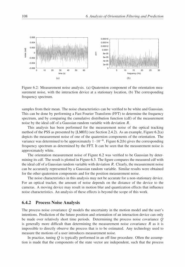
108 6. Analysis of Orientation Filtering and Prediction
-0.006
-0.004
-0.002
0
0.002
0.004
0.006
0 10 20 30 40 50 60
nois
e (
rad)
time (s)
(a)
0
2e-05
4e-05
6e-05
8e-05
0.0001
0.00012
0.00014
0.00016
5 10 15 20 25 30
FF
T
frequency (Hz)
(b)
Figure 6.2: Measurement noise analysis. (a) Quaternion component of the orientation mea-
surement noise, with the interaction device at a stationary location, (b) The corresponding
frequency spectrum.
samples from their mean. The noise characteristics can be verified to be white and Gaussian.
This can be done by performing a Fast Fourier Transform (FFT) to determine the frequency
spectrum, and by comparing the cumulative distribution function (cdf) of the measurement
noise by the ideal cdf of a Gaussian random variable with deviation R.
This analysis has been performed for the measurement noise of the optical tracking
method of the PSS as presented by [LM03] (see Section 2.4.2). As an example, Figure 6.2(a)
depicts the measurement noise of one of the quaternion components of the orientation. The
variance was determined to be approximately 1 � 10�6. Figure 6.2(b) gives the corresponding
frequency spectrum as determined by the FFT. It can be seen that the measurement noise is
approximately white.
The orientation measurement noise of Figure 6.2 was verified to be Gaussian by deter-
mining its cdf. The result is plotted in Figure 6.3. The figure compares the measured cdf with
the ideal cdf of a Gaussian random variable with deviation R. Clearly, the measurement noise
can be accurately represented by a Gaussian random variable. Similar results were obtained
for the other quaternion components and for the position measurement noise.
The noise characteristics in this analysis may not be accurate for a non-stationary device.
For an optical tracker, the amount of noise depends on the distance of the device to the
cameras. A moving device may result in motion blur and quantization effects that influence
noise characteristics. An analysis of these effects is beyond the scope of this work.
6.4.2 Process Noise Analysis
The process noise covariance Q models the uncertainty in the motion model and the user’s
intentions. Prediction of the future position and orientation of an interaction device can only
be made over relatively short time periods. Determining the process noise covariance Q
is generally more difficult than determining the measurement noise covariance R as it is
impossible to directly observe the process that is to be estimated. Any technology used to
measure the motions of a user introduces measurement noise.
In practice, tuning Q is typically performed in an off-line procedure. Often the assump-
tion is made that the components of the state vector are independent, such that the process

6.5. Test Procedure 109
0
0.2
0.4
0.6
0.8
1
0.708 0.71 0.712 0.714 0.716
CD
F
angle
measuredideal
Figure 6.3: Cumulative distribution function of the orientation measurement noise.
noise covariance matrix Q is diagonal. For the orientation state vector of Equation 6.8 this
implies that orientation and angular velocity must be independent. In this case, Q can be
described by 7 parameters, which can be further reduced to 2 parameters by assuming that
the quaternion components and the angular velocity components are identical.
In case the process to be estimated can be observed directly such that a reference sig-
nal can be obtained, the process noise covariance Q can be determined using a non-linear
optimization routine that optimizes the filter’s output to match the reference signal.
6.5 Test Procedure
6.5.1 Signal characteristics
Experimental versus Synthetic Motion Data
A filter and prediction comparison can be performed on experimental or synthetic motion
data. Since the goal of this work is to evaluate performance in a VR context, motion data
of typical VR tasks is needed. The easiest way to obtain such data is through a series of
experiments, where users are asked to perform some task while their movements are recorded.
The main problem with this approach is that the original signal is unknown, as only noisy
measurement data is available. It is possible to clean up the data to some extent and use this
as a reference signal, but this needs great care to avoid introducing false signal characteristics
or removing true ones.
An alternative would be to use a setup that can generate a known and controllable motion.
For instance, a pendulum could be used to generate a motion with accurately known charac-
teristics. By equipping this pendulum with markers, filtered pose estimates from the tracking
system can be compared to the motion of the pendulum. However, the resulting motion char-
acteristics do not model hand motions in VR tasks. Furthermore, they are highly repetitive,
such that the Bayesian filtering methods converge towards steady-state.
Another approach would be to use synthetic signals. However, it is extremely difficult to
model the exact characteristics of hand motions encountered in VR tasks. A filter compari-
son, using synthetic signals that have little in common with the signals encountered during a
typical VR interactive session, would say little about performance in a VR context.
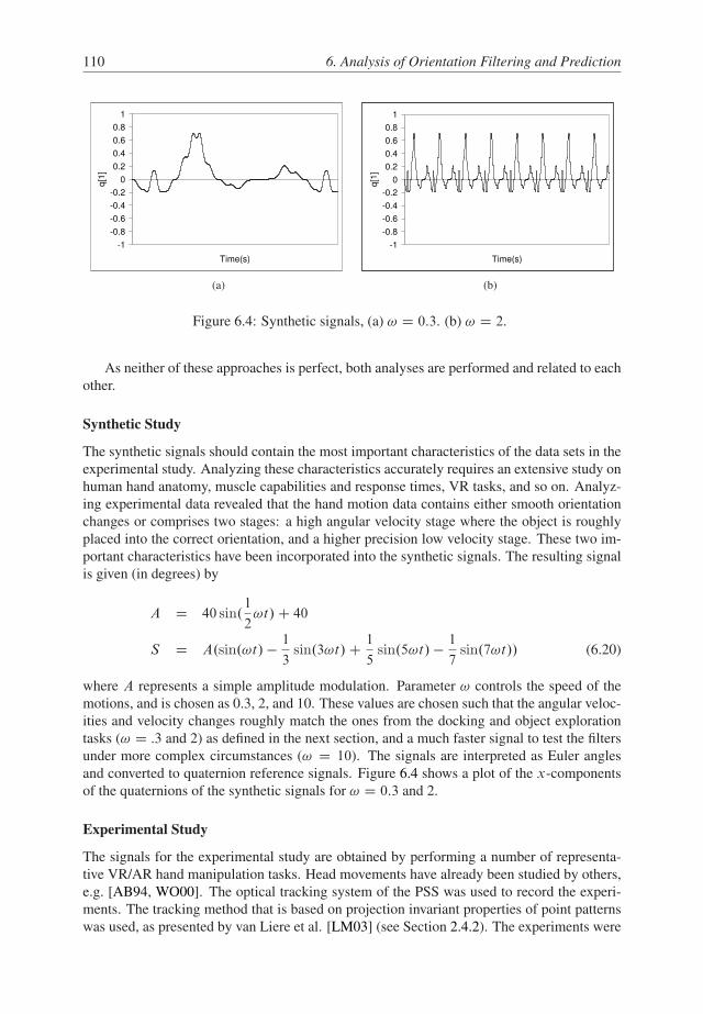
110 6. Analysis of Orientation Filtering and Prediction
-1
-0.8
-0.6
-0.4
-0.2
0
0.2
0.4
0.6
0.8
1
Time(s)
q[1
]
(a)
-1
-0.8
-0.6
-0.4
-0.2
0
0.2
0.4
0.6
0.8
1
Time(s)
q[1
]
(b)
Figure 6.4: Synthetic signals, (a) ! D 0:3. (b) ! D 2.
As neither of these approaches is perfect, both analyses are performed and related to each
other.
Synthetic Study
The synthetic signals should contain the most important characteristics of the data sets in the
experimental study. Analyzing these characteristics accurately requires an extensive study on
human hand anatomy, muscle capabilities and response times, VR tasks, and so on. Analyz-
ing experimental data revealed that the hand motion data contains either smooth orientation
changes or comprises two stages: a high angular velocity stage where the object is roughly
placed into the correct orientation, and a higher precision low velocity stage. These two im-
portant characteristics have been incorporated into the synthetic signals. The resulting signal
is given (in degrees) by
A D 40 sin.1
2!t/C 40
S D A.sin.!t/ � 1
3sin.3!t/C 1
5sin.5!t/ � 1
7sin.7!t// (6.20)
where A represents a simple amplitude modulation. Parameter ! controls the speed of the
motions, and is chosen as 0.3, 2, and 10. These values are chosen such that the angular veloc-
ities and velocity changes roughly match the ones from the docking and object exploration
tasks (! D .3 and 2) as defined in the next section, and a much faster signal to test the filters
under more complex circumstances (! D 10). The signals are interpreted as Euler angles
and converted to quaternion reference signals. Figure 6.4 shows a plot of the x-components
of the quaternions of the synthetic signals for ! D 0:3 and 2.
Experimental Study
The signals for the experimental study are obtained by performing a number of representa-
tive VR/AR hand manipulation tasks. Head movements have already been studied by others,
e.g. [AB94, WO00]. The optical tracking system of the PSS was used to record the experi-
ments. The tracking method that is based on projection invariant properties of point patterns
was used, as presented by van Liere et al. [LM03] (see Section 2.4.2). The experiments were

6.5. Test Procedure 111
(a) (b)
Figure 6.5: Screenshot of two experiments. (a) Tracing task. The goal is to trace the contour
with the ring, without the contour and ring colliding at any point. The ring is manipulated
using a cube-shaped interaction device. (b) Docking task. The goals is to dock the left cube,
which is manipulated using the same interaction device, into the target cube on the right.
performed using a cubic interactive device. In order to obtain angular velocity measurements,
the device was also equipped with an inertial measurement unit, the Xsens MT9 [XSE]. The
unit communicates through RS-232 and provides access to its gyroscopes.
Complex hand manipulation tasks are commonly regarded as combinations of four basic
tasks [BKLP01]: selection, manipulation, navigation and system control. The following hand
tasks were performed, which represent the motions of the basic tasks:
� Selection
A target sphere is drawn at a random location. At the location of a cubic-shaped inter-
action device a source sphere is drawn. The goal is to place the source sphere over the
target sphere. If the task is completed, the target is highlighted, after which the user
presses a pedal to repeat the experiment.
� Tracing
A contour is plotted and the user controls a ring with the interaction device. The user
has to trace the contour with the ring, without the ring and contour colliding. This
experiment is shown in Figure 6.5(a).
� Docking
A target box is drawn with a random orientation. The box is drawn with differently
colored spheres at the corners. An identical box is drawn with the same position and
orientation as the interaction device. The goal is to align the source and target boxes.
If the task is completed, the target is highlighted and the user presses a pedal to repeat
the experiment. A screenshot of this experiment is given in Figure 6.5(b).
� Object exploration
A cube is drawn with the same position and orientation of the input device. Each side
of the cube has a different color. The goal is to orient the cube such that the side with a
randomly given color faces the user, after which a pedal is pressed and the experiment
repeated.

112 6. Analysis of Orientation Filtering and Prediction
-1
-0.8
-0.6
-0.4
-0.2
0
0.2
0.4
0.6
0.8
1
Time (s)
q[1
]
(a)
-1
-0.8
-0.6
-0.4
-0.2
0
0.2
0.4
0.6
0.8
1
Time (s)
q[1
]
(b)
-1
-0.8
-0.6
-0.4
-0.2
0
0.2
0.4
0.6
0.8
1
Time (s)
q[1
]
(c)
-1
-0.8
-0.6
-0.4
-0.2
0
0.2
0.4
0.6
0.8
1
Time (s)
q[1
]
(d)
Figure 6.6: Experimental input signals. (a) selection, (b) tracing, (c) docking, (d) object
exploration.
Each task was performed a number of times by one user with VR experience. Since the
resulting signals are used as input to the filters, task completion times and success rates are not
relevant. Each data set is cut to 50 seconds in length. As an example, the x-components of the
quaternions are shown in Figure 6.6. The selection task produces a signal with a small range
of orientations, where the orientation changes fast when changing selections and is practically
constant in between. The tracing task produces a slightly more complex signal with a larger
range of orientations and angular velocities. The docking task produces the entire range of
orientations and a mix of high and low angular velocities. The signal clearly demonstrates
a fast initial orientation change, followed by the slow more precise task of the final docking
procedure. The object exploration task also shows the entire range of orientations and the
largest angular velocities and accelerations. Comparing these signals with the head motion
data sets from [AB94], it can be concluded that these hand tasks result in a larger range of
signal characteristics.
Obtaining a Reference Signal
To be able to compare the performance of the prediction methods, the true signal is needed.
Since this signal is not available for an experimental study, the approach of Azuma was
followed [Azu95]: a high order non-causal low-pass filter was applied to the measured signal
to obtain a reference or “ground truth” signal. The filter is carefully tuned to filter out most
of the measurement noise, while keeping the original signal characteristics in tact. It was

6.5. Test Procedure 113
-0.65
-0.64
-0.63
-0.62
-0.61
-0.6
0 20 40 60 80 100
q[0
]
frame
cleanmeasured
Figure 6.7: Results of the non-causal low-pass filter that is used to obtain a reference signal.
informally observed that higher frequency components in the original signal practically never
exceed 10 Hz. Although the resulting reference signal may still contain a small amount of
sensor noise, this noise is brought to a minimum. Moreover, it is virtually impossible to
discriminate between lower frequency sensor noise and normal hand jittering. To examine
the influence of noise on the relative performance of the filter methods, artificial noise was
added to the reference signal of different magnitudes. The result of running the non-causal
low-pass filter on motion data is shown in Figure 6.7. The figure illustrates the cleaning
capability of the filter, without introducing extra lag or overshoot.
The tasks defined in Section 6.5.1 were recorded a number of times, and the ones that
contained a minimal amount of measurement errors were selected. Measurement errors were
found by inspection of the generated signals. Recordings with invalid spikes were rejected.
These precautions minimize the number of false characteristics introduced to the true signal.
A possible constant measurement bias does not really affect the characteristics of the original
signal. Since each filter is tuned so that its output maximally matches the reference signal,
such a bias has no influence on this relative performance study. For an absolute performance
study of a filter, these arguments do not apply.
6.5.2 Performance Metrics
The accuracy of a filtering method is defined as the root mean square error (RMSE) of the
difference in orientation between the filtered and reference signal in degrees
RMSE D
v
u
u
t
1
N
NX
iD1
.360
�cos�1..qci
� q�1ei
/w//2 (6.21)
where qe is the quaternion representing the estimated orientation, qc represents the reference
signal, and qw represents the w-component of quaternion q. Since the RMSE only gives an
idea of the accuracy of a filter over the entire length of the data set, the peak error of the
orientation mismatch in degrees is also analyzed. Large peak errors can be very disturbing in
VR/AR environments and therefore are an important error metric.
Furthermore, an improvement factor is defined, which indicates how effective the use of

114 6. Analysis of Orientation Filtering and Prediction
a filtering method is, compared to directly using the measurements:
Improvement factor D RMSEno f iltering
RMSEf iltered
(6.22)
6.5.3 System Parameters
The tracking system introduces various parameters that influence the performance of predic-
tion schemes. The first system parameter is the sampling frequency fs . The optical tracking
system operates at a frequency fs D 60 Hz. Since many popular tracking sensors, such as
the Polhemus, the Logitech Acoustical tracker, and many optical tracking systems, operate
at comparable or lower frequencies, fs is only lowered by downsampling the data set. Al-
though upsampling is possible to obtain higher sampling frequencies, characteristics of the
true signal that may have been missed by sampling at 60 Hz cannot be added reliably without
exact knowledge of this signal. The synthetic signal is also sampled at 60 Hz. All data sets
are sampled at 60, 30, 20, and 15 Hz.
The second system parameter is the measurement noise Nz . The variances of the steady-
state orientation and angular velocity measurement noise components were obtained as de-
scribed in Section 6.4, which are approximations of the true measurement noise. The ob-
tained values are �2 D 10�6 and �2 D 9 � 10�4, respectively. Gaussian random noise was
then added to the reference data sets, of magnitudes 1, 10, and 100 times the orientation mea-
surement noise (renormalizing the resulting quaternion), and 1, 3, and 9 times the angular
velocity measurement noise. Although the measurement noise of the optical tracker depends
on the distance to the cameras and is far less in the center of the workspace, these values
were regarded as constant and identical, since this study is a relative filter performance study.
Absolute filter performance can be increased by a more accurate noise model.
The last parameter is the prediction time tpred . This parameter is directly related to the
end-to-end delay of the system, t2 � t1 in Figure 6.1. The prediction time was varied from
0 (i.e. only filtering) to 100 ms in steps of 33 ms. The errors at higher prediction times
generally become too large for practical use [AB94].
6.6 Results
6.6.1 Synthetic Study
The EKF, UKF and LTI filters were applied to the synthetic signals. In Section 6.5.3, the
settings of the parameters are defined. The filters were ran on each parameter combination,
using the motion model including inertial measurements. The particle filters were ran on
a subset of the parameter space for faster simulation. The most important results of the
experiments are presented below.
� Filtering and measurement noise
The improvement factor of each filter method for increasing measurement noise is
graphed in Figure 6.8(a), where tpred D 0 ms and ! D 2 (see Equation 6.20). The
improvement factor versus task is depicted in Figure 6.8(b).
� Prediction time
The results of increasing the prediction time are graphed in Figure 6.9. Here, the RMSE
and peek error are plotted versus prediction time, for ! D 2.

6.6. Results 115
0
1
2
3
4
5
6
7
1 10 100Measurement Noise
Impro
vem
ent F
acto
r
EKF UKF EPF UPF
(a)
0
0.5
1
1.5
2
2.5
3
3.5
4
0.3 2 10
omega
Imp
rove
me
nt
Fa
cto
r
EKF UKF EPF UPF
(b)
Figure 6.8: Synthetic results for filtering (tpred D 0): (a) Improvement factor vs. measure-
ment noise (! D 2). (b) Improvement factor vs. omega for 10 times Nz .
0
5
10
15
20
25
30
0 33 66 100Prediction time (ms)
RM
SE
(d
eg
)
EKF UKF EPF UPF No prediction
(a)
0
10
20
30
40
50
60
70
80
90
100
0 33 66 100Prediction time (ms)
Pe
ek e
rro
r (d
eg
)
EKF UKF EPF UPF No prediction
(b)
Figure 6.9: Synthetic results for prediction (! D 2): (a) RMSE vs. prediction time. (b) Peek
error vs. prediction time.

116 6. Analysis of Orientation Filtering and Prediction
0
2
4
6
8
10
12
14
16
18
60 30 20 15Sampling frequency (Hz)
RM
SE
(deg)
EKF UKF EPF UPF No prediction
(a)
0
10
20
30
40
50
60
70
60 30 20 15Sampling frequency (Hz)
Pe
ek e
rro
r (d
eg
)
EKF UKF EPF UPF No prediction
(b)
Figure 6.10: Synthetic results for sampling frequency (! D 0:3): (a) RMSE vs. sampling
frequency. (b) Peek error vs. sampling frequency.
� Sampling frequency
The sampling frequency versus RMSE and peek error is shown in Figure 6.10. The
figure shows the results for ! D 0:3, a prediction time of 66 ms, and the measurement
noise at its nominal value. The influence of fs on the peak error is similar to the RMSE.
� Relative filter performance
The performance results of the predictive methods are graphed in Figure 6.11. Here,
the prediction time is 66 ms, the sampling frequency 60 Hz, and the measurement noise
10 and 3 times its nominal values. The results are shown for ! at 0.3, 2, and 10. The
particle filters each used 50 particles.
6.6.2 Experimental Study
For the experimental study the same analysis was performed as in the synthetic, except both
motion models are used. This results in 384 combinations for each filter. The most important
results are given below, which are very similar to the synthetic case.
� Filtering and measurement noise
The results of filtering (i.e. tpred D 0 ms) are graphed in Figure 6.12. Figure 6.12(a)
shows the improvement factor of each filter for increasing measurement noise, using
the docking task and the MM model. Figure 6.12(b) shows the improvement factor of
each filter for each task, with a measurement noise of 10 times its nominal value. The
peak error shows similar behavior as the RMSE, where the exploration and docking
tasks give slightly higher values than no filtering, with the measurement noise at both
nominal and 10.

6.7. Discussion 117
0
10
20
30
40
50
60
.3 2 10omega
RM
SE
(d
eg
)
EKF UKF EPF UPF No prediction
Figure 6.11: Synthetic results: Filter comparison for tpred D 66 ms, fs D 60 Hz, Nz 10 and
3 times the nominal orientation and angular velocity measurement noise.
� Prediction time
The results of increasing the prediction time are graphed in Figure 6.13. Figure 6.13(a)
plots the RMSE versus prediction time using the docking task, whereas Figure 6.13(b)
depicts the peek error versus prediction time. Figure 6.14 shows the improvement
factor using the object exploration task. The results are for the MM model.
� Sampling frequency
The effects of changing the sampling frequency fs are shown in Figure 6.15. The
figure shows the results of the docking task for the prediction time at 66 ms and the
measurement noise at its nominal value, using the MM model. The influence of fs on
the peak error is similar to the RMSE.
� Relative filter performance
The performance results of the predictive filtering methods are given for the prediction
time at 66 ms, the sampling frequency at 60 Hz, and the measurement noise as 10 and
3 times the nominal value of the orientation and angular velocity measurement noise,
respectively. Figure 6.16 shows the RMSE values for each task, using both system
models. The particle filters each used 50 particles. Larger numbers of particles gave
no further improvement.
6.7 Discussion
Filtering and Measurement Noise
The experimental results in Figure 6.12 show that for increasing measurement noise Nz , the
improvement factor of each filter relative to no filtering increases. The EKF and UKF have
similar performance, while the LTI only gives an improvement over no prediction when Nz

118 6. Analysis of Orientation Filtering and Prediction
0
0,5
1
1,5
2
2,5
3
3,5
1 10 100Measurement Noise
Imp
rove
me
nt F
acto
r
LTI EKF UKF EPF UPF
(a)
0
0,5
1
1,5
2
2,5
Select Trace Dock ExploreTask
Imp
rove
me
nt
Fa
cto
r
LTI EKF UKF EPF UPF
(b)
Figure 6.12: Filter results: (a) Improvement factor vs. measurement noise (docking task). (b)
Improvement factor vs. task for 10 times Nz .
0
1
2
3
4
5
6
0 33 66 100Prediction time (ms)
RM
SE
(d
eg
)
LTI EKF UKF
EPF UPF No prediction
(a)
0
5
10
15
20
25
0 33 66 100Prediction time (ms)
Peek e
rror
(deg)
LTI EKF UKF
EPF UPF No prediction
(b)
Figure 6.13: Prediction results (docking task): (a) RMSE vs. prediction time. (b) Peek error
vs. prediction time.

6.7. Discussion 119
0
0,2
0,4
0,6
0,8
1
1,2
1,4
1,6
1,8
2
0 33 66 100Prediction time (ms)
Impro
vem
ent fa
cto
r
LTI EKF UKF EPF UPF
Figure 6.14: Prediction results (docking task): Improvement factor vs. prediction time (ex-
ploration task)
0
0,5
1
1,5
2
2,5
3
3,5
4
60 30 20 15Sampling frequency (Hz)
RM
SE
(d
eg
)
LTI EKF UKF EPF UPF No prediction
(a)
0
2
4
6
8
10
12
14
16
18
60 30 20 15Sampling frequency (Hz)
Pe
ek e
rro
r (d
eg
)
LTI EKF UKF EPF UPF No prediction
(b)
Figure 6.15: RMSE and peek error vs. sampling frequency for tpred D 66 ms, Nz nominal.

120 6. Analysis of Orientation Filtering and Prediction
0
2
4
6
8
10
12
14
Select Trace Dock ExploreTask
RM
SE
(d
eg
)
LTI EKF UKF EPF UPF No prediction
(a)
0
2
4
6
8
10
12
14
Select Trace Dock ExploreTask
RM
SE
(d
eg
)
EKF UKF EPF UPF No prediction
(b)
Figure 6.16: Filter comparison for tpred D 66 ms, fs D 60 Hz, Nz 10 and 3 times the
nominal orientation and angular velocity measurement noise, respectively, using (a) only
orientation measurements (MM), and (b) including inertial measurements (MMI).
is sufficiently high. For a measurement noise 100 times its nominal value, the LTI performs
significantly worse than the EKF and UKF. This is caused by the small filter kernel. It might
be solved using a slightly larger filter kernel, but this also introduces more lag which needs
to be compensated.
Figure 6.12(b) suggests that as a signal’s complexity increases, using a filtering method
becomes less effective. This is likely the result of the process model being less accurate for
more erratic motions.
Figure 6.8(a) confirms the results of the experimental study, showing that the effectiveness
of the Bayesian filtering methods increases with measurement noise.
Prediction Time
Figure 6.13 shows a practically linear dependency between the RMSE and the prediction time
for tpred � 33 ms. The peek error shows similar characteristics. This implies that the system
latency t2 � t1 (see Figure 6.1) should be kept as small as possible. The performance of the
EKF and UKF are similar, while the LTI scores only slightly less. The figure further suggests
that the improvement factor reaches an optimal value for a prediction time between 33 and
66 ms, and decreases as the prediction time is further increased. Application of a predictive
filtering method is about 1.7 times less effective for a prediction time of 0 ms, compared to
33 ms.
Figure 6.8(b) shows that the RMSE increases fast with increasing prediction time, much
worse than the almost linear dependency of Figure 6.14. The uncertainty of the motion model
increases with prediction time, which is reflected in a much higher process noise. It is to be
expected that at a certain prediction time, the process noise becomes so large that the filters
regard the measurements to be more accurate, and the improvement factor converges to 1.
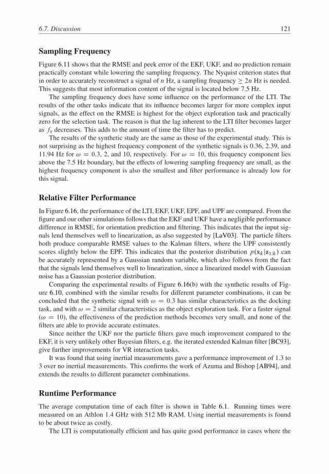
6.7. Discussion 121
Sampling Frequency
Figure 6.11 shows that the RMSE and peek error of the EKF, UKF, and no prediction remain
practically constant while lowering the sampling frequency. The Nyquist criterion states that
in order to accurately reconstruct a signal of n Hz, a sampling frequency � 2n Hz is needed.
This suggests that most information content of the signal is located below 7.5 Hz.
The sampling frequency does have some influence on the performance of the LTI. The
results of the other tasks indicate that its influence becomes larger for more complex input
signals, as the effect on the RMSE is highest for the object exploration task and practically
zero for the selection task. The reason is that the lag inherent to the LTI filter becomes larger
as fs decreases. This adds to the amount of time the filter has to predict.
The results of the synthetic study are the same as those of the experimental study. This is
not surprising as the highest frequency component of the synthetic signals is 0.36, 2.39, and
11.94 Hz for ! D 0:3, 2, and 10, respectively. For ! D 10, this frequency component lies
above the 7.5 Hz boundary, but the effects of lowering sampling frequency are small, as the
highest frequency component is also the smallest and filter performance is already low for
this signal.
Relative Filter Performance
In Figure 6.16, the performance of the LTI, EKF, UKF, EPF, and UPF are compared. From the
figure and our other simulations follows that the EKF and UKF have a negligible performance
difference in RMSE, for orientation prediction and filtering. This indicates that the input sig-
nals lend themselves well to linearization, as also suggested by [LaV03]. The particle filters
both produce comparable RMSE values to the Kalman filters, where the UPF consistently
scores slightly below the EPF. This indicates that the posterior distribution p.xk jz1Wk/ can
be accurately represented by a Gaussian random variable, which also follows from the fact
that the signals lend themselves well to linearization, since a linearized model with Gaussian
noise has a Gaussian posterior distribution.
Comparing the experimental results of Figure 6.16(b) with the synthetic results of Fig-
ure 6.10, combined with the similar results for different parameter combinations, it can be
concluded that the synthetic signal with ! D 0:3 has similar characteristics as the docking
task, and with ! D 2 similar characteristics as the object exploration task. For a faster signal
(! D 10), the effectiveness of the prediction methods becomes very small, and none of the
filters are able to provide accurate estimates.
Since neither the UKF nor the particle filters gave much improvement compared to the
EKF, it is very unlikely other Bayesian filters, e.g. the iterated extended Kalman filter [BC93],
give further improvements for VR interaction tasks.
It was found that using inertial measurements gave a performance improvement of 1.3 to
3 over no inertial measurements. This confirms the work of Azuma and Bishop [AB94], and
extends the results to different parameter combinations.
Runtime Performance
The average computation time of each filter is shown in Table 6.1. Running times were
measured on an Athlon 1.4 GHz with 512 Mb RAM. Using inertial measurements is found
to be about twice as costly.
The LTI is computationally efficient and has quite good performance in cases where the

122 6. Analysis of Orientation Filtering and Prediction
LTI EKF UKF EPF UPF
MM 13 �s 47 �s 215 �s 2.05 ms 11.7 ms
MMI - 77 �s 392 �s 4.1 ms 21.4 ms
Table 6.1: Average running times per frame
measurement noise is not too high, and sampling frequency is sufficiently high. However, it
is far more sensitive to measurement noise and sampling frequency than the Bayesian filters.
Moreover, the prediction time to compensate for its lag and the length of the history used
to calculate the angular velocity were optimized for each specific simulation. These tuning
parameters depend on the characteristics of the input signal and the parameters involved, and
may need to be adaptive. Alternatively, quaternion-based extrapolation techniques may prove
to be effective for prediction.
The EKF requires the derivation of Jacobian matrices which generally makes its imple-
mentation more complex. Although the UKF does not require this derivation, the algorithm
is somewhat more complex, requiring the calculation of a matrix square root (which can be
calculated through a Cholesky factorization). As the derivation of the Jacobian matrices is
a simple task for the motion model in this work, the EKF is easier to implement. Given its
lower computation time and the fact that the computationally more expensive particle filters
do not give more accurate results, the use of an EKF is sufficient for orientation prediction
under the given circumstances.
Parameter Determination
As discussed in Section 6.5, the filters were tuned specifically for each simulation. Testing
showed that the tuning parameters for the motion model Fk in Figure 6.1 vary significantly
between input signals and different filter parameters. Incorrect parameters can lead to worse
performance than using no filtering or prediction at all, and may even lead to completely
‘loosing track’. Adaptive or self-tuning approaches, such as multimodal filtering, residual
whitening and dual extended Kalman filtering [CNHV99, May79] may be promising tech-
niques to improve filter performance and its application in practice.
RMSE versus Covariance
For this relative performance RMSE was chosen as performance measure. An alternative
method to examine filter performance is the use of the covariance matrices generated by the
filters. The diagonal terms of the covariance matrices represent the variances of the estimation
errors of the state. For non-linear systems these only approximate the actual estimation error
covariance. Since the covariance matrices still give a good indication of the general trend of
the estimation error variances of the state, they were included in the analysis.
Figure 6.17 plots the trace of the covariance matrix generated by the EKF versus the
MSE as a function of time, for the docking task, tpred D 66 ms, fs D 60 Hz and Nz 10.
Other runs and filters gave similar results. Visually comparing both figures shows that the
estimation error computed by the covariance matrix is correlated with the RMSE. A better
approach to compare both figures would be to perform a correlation analysis, however, this
will give similar results. Filter consistency has been confirmed by normalized innovation and
state estimation error tests, as described in [BSF88].
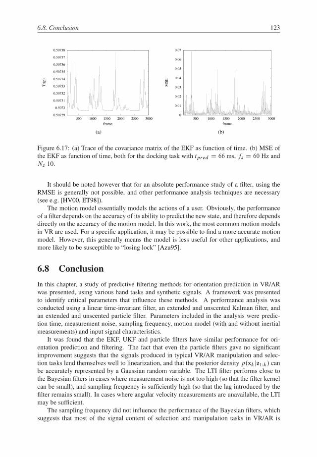
6.8. Conclusion 123
0.50729
0.5073
0.50731
0.50732
0.50733
0.50734
0.50735
0.50736
0.50737
0.50738
500 1000 1500 2000 2500 3000
Tr(
p)
frame
(a)
0
0.01
0.02
0.03
0.04
0.05
0.06
0.07
500 1000 1500 2000 2500 3000
MS
E
frame
(b)
Figure 6.17: (a) Trace of the covariance matrix of the EKF as function of time. (b) MSE of
the EKF as function of time, both for the docking task with tpred D 66 ms, fs D 60 Hz and
Nz 10.
It should be noted however that for an absolute performance study of a filter, using the
RMSE is generally not possible, and other performance analysis techniques are necessary
(see e.g. [HV00, ET98]).
The motion model essentially models the actions of a user. Obviously, the performance
of a filter depends on the accuracy of its ability to predict the new state, and therefore depends
directly on the accuracy of the motion model. In this work, the most common motion models
in VR are used. For a specific application, it may be possible to find a more accurate motion
model. However, this generally means the model is less useful for other applications, and
more likely to be susceptible to “losing lock” [Azu95].
6.8 Conclusion
In this chapter, a study of predictive filtering methods for orientation prediction in VR/AR
was presented, using various hand tasks and synthetic signals. A framework was presented
to identify critical parameters that influence these methods. A performance analysis was
conducted using a linear time-invariant filter, an extended and unscented Kalman filter, and
an extended and unscented particle filter. Parameters included in the analysis were predic-
tion time, measurement noise, sampling frequency, motion model (with and without inertial
measurements) and input signal characteristics.
It was found that the EKF, UKF and particle filters have similar performance for ori-
entation prediction and filtering. The fact that even the particle filters gave no significant
improvement suggests that the signals produced in typical VR/AR manipulation and selec-
tion tasks lend themselves well to linearization, and that the posterior density p.xk jz1Wk/ can
be accurately represented by a Gaussian random variable. The LTI filter performs close to
the Bayesian filters in cases where measurement noise is not too high (so that the filter kernel
can be small), and sampling frequency is sufficiently high (so that the lag introduced by the
filter remains small). In cases where angular velocity measurements are unavailable, the LTI
may be sufficient.
The sampling frequency did not influence the performance of the Bayesian filters, which
suggests that most of the signal content of selection and manipulation tasks in VR/AR is
124 6. Analysis of Orientation Filtering and Prediction
located below 7.5 Hz. This does not mean a sampling rate of 15 Hz is sufficient, as the human
perception system perceives an update rate of 15 Hz to be ‘jerky’. Moreover, Azuma and
Bishop have shown [AB94] that the prediction time must in fact be kept below 80 ms, since
predicted output signals have more energy in higher frequency bands, increasing perceived
jittering.
Further conclusions are that the application of a filtering method is most effective for
a prediction time between 33 and 66 ms, and becomes less effective for higher prediction
times. The improvement factor over no filtering increases as measurement noise increases
and shows a dependency with the complexity of the input signal.
The tuning parameters of the filters varied significantly with changing input signals and
filter parameters as prediction time. In practice, parameters as prediction time and sampling
frequency are fixed, and the most significant influence on tuning parameters is the type of
task. Adaptive filtering may provide a solution to this problem, such that the tuning param-
eters are automatically adjusted. One approach is to use multiple motion models, which are
tuned to different types of motions [CNHV99]. Another possibility would be to control the
tuning parameters based on the task a user is performing in the application. Consequently,
high-level interaction information would be exploited in a low-level filtering and prediction
method.
In these studies, measurement noise was modeled as additive Gaussian noise. Although
the steady state noise of the optical tracking system was confirmed to be additive Gaussian,
the measurement noise depends on the position of the input device relative to the cameras.
Measurement noise increases as a function of the distance to the cameras. In case of an
optical tracking system, a more accurate way to model the measurement process would be
to include the steps used to calculate an orientation from 2D marker positions. However,
since highly accurate measurement models are not available for all tracking systems, the
measurement model was simplified. More accurate modeling of the measurement process
and the measurement noise can further increase filter and prediction performance.
More research is needed to accurately model hand motion characteristics in a VR envi-
ronment. Such a model can be used to create synthetic signals that act as a performance
benchmark for filter and prediction performance evaluation, and to develop more accurate
motion models for the filtering techniques.

Chapter 7
Tracking and Model Estimation of
Composite Interaction Devices
Chapters 3 and 4 focussed on tracking and model estimation of rigid interaction devices.
Chapter 6 aimed at improving the pose estimate provided by these tracking techniques with
respect to noise and latency. Although rigid devices are applicable in a number of areas,
some tasks require the manipulation of a larger number of dimensions. Consider for instance
a modeling application, which includes spatial manipulation tasks as positioning, orienting,
and scaling. In case of uniform scaling, the number of input dimensions is 7, while this
number increases to 9 in case of non-uniform scaling. A six degree of freedom input device
does not provide enough dimensions to perform such tasks without mode switching. An
alternative approach would be to use an interaction device that supports the manipulation of
a larger number of input dimensions.
The goal of this chapter is to develop a tracking system that allows a developer to rapidly
construct and apply composite interaction devices. Composite interaction devices consist of
linked segments with degrees of freedom with respect to each other. An example composite
interaction device would be a glove, where the palm of the hand defines a six degree of
freedom reference frame, and where each segment corresponds to a finger segment with
rotational degrees of freedom with respect to each other. Composite interaction devices open
up new perspectives on interaction in VR, as well as being applicable in a number of related
research areas, such as medical research, animation, and rehabilitation.
The difficulty in tracking composite interaction devices is that each segment needs to be
recognized. A simple approach would be to equip each segment with enough markers to be
able to use the tracking techniques of Chapters 3 or 4 to recognize each segment separately.
However, the resulting interaction devices would be prohibitively large for use in a desktop
virtual environment such as the PSS.
In this chapter, a model-based optical tracking and automatic model estimation system for
composite interaction devices is developed. Composite interaction devices are defined as ob-
jects that consist of a hierarchy of linked segments, where each segment can have degrees of
freedom (DOFs) relative to a parent segment. Devices consist of one reference segment that
is equipped with multiple markers, while other segments can contain only a single marker.
This keeps the devices compact and easy to handle. The goal of this chapter is to develop
tracking techniques for such devices and model estimation techniques to automatically de-
rive the skeleton structure of these devices from motion data, along with the DOFs of each
segment relative to its parent.
125

126 7. Tracking and Model Estimation of Composite Interaction Devices
Figure 7.1: The tracking and model estimation system for composite interaction devices.
7.1 Overview
In this chapter, a model-based optical tracking and automatic model estimation system for
composite interaction devices is presented. The system is designed to support a low num-
ber of markers attached to each segment, such that small interaction devices can be used
in the virtual environment. Furthermore, the system is able to automatically estimate a hi-
erarchical model of the interaction device from motion capture data, describing the DOF
relations between segments, their ranges, and the geometric skeleton structure defining how
these segments are connected. The optical tracking system is able to use the obtained mod-
els to identify the devices, and to determine all DOF parameters describing the pose of each
segment.
Most previous work on model estimation of composite interaction devices has focussed
on the human body. Each limb is either equipped with at least three markers (e.g. [HSDK05]),
or models need to be pre-defined. By giving each segment a unique configuration of three or
more markers, segments can be easily identified and a full coordinate system can be derived
from the marker configuration. Examining the relation between segments is then reduced to
examining the relation between moving coordinate systems. Clearly, this approach does not
work when segments are allowed to contain less than three markers. Many VR systems, and
desktop virtual environments in particular, work with interaction devices much smaller than
the human body. As a result, segments of the interaction device may not provide enough
room to accommodate multiple markers.
For the model estimation techniques presented in this chapter, it is assumed that stereo
and frame-to-frame correspondence have been performed, resulting in labeled 3D marker
locations. The techniques to achieve this are described in Chapter 4. The model estimation
and tracking system for composite interaction devices is outlined in Figure 7.1.
Model estimation works in three steps:
� First, rigid objects are identified. These are objects that are equipped with three or more
markers. A model of such objects is obtained using the model estimation techniques
described in Chapter 4.

7.1. Overview 127
(a) (b)
Figure 7.2: (a) An example composite interaction device. The hand consists of a reference
segment with 6 markers, followed by single marker segments with rotational DOFs. (b) The
corresponding model with the 3D marker locations, skeleton structure, DOF relations and
ranges, and reference frames.
� A model of single marker segments is obtained, which describes the DOFs and their
ranges of each segment, relative to a frame of reference. This procedure is based on ex-
amining the geometric shape that the moving marker describes. For instance, a marker
on a segment with one rotational DOF with respect to a parent segment results in a
3D circle arc. A set of fitting routines is applied to determine the geometric shape
which best describes the motion of a single marker. Next, the parameters describing
this geometric shape are mapped to the parameters of the corresponding DOF model.
A new local coordinate system is constructed in the single marker segment, according
to the determined DOF relation. This coordinate system functions as a new reference
coordinate system to find other relations.
� After all possible DOF relations between segments are determined, a skeleton estima-
tion procedure is used to derive the final hierarchical structure of the segments of the
device.
As an example, Figure 7.2 shows a finger, along with the model as determined by the
model estimation method. The finger features four segments, one used as a six DOF reference
coordinate system (the palm), followed by a single marker segment with two rotational DOFs
(the proximal phalanx) and two segments with each one rotational DOF (the middle and distal
phalanges). During model estimation, the user moves the various parts of the composite
interaction device in front of the cameras, such that all markers can be seen. Markers that
are occluded for a short period of time are handled during frame-to-frame correspondence by
predicting occluded markers locations (see Chapter 4). Long-term partial occlusion is only
allowed in segments with more than three markers.
The tracking system is based on the following steps:

128 7. Tracking and Model Estimation of Composite Interaction Devices
� The model obtained from the model estimation techniques is used to determine the
pose of the interaction device, using the rigid body tracking techniques presented in
Chapter 4.
� Markers are mapped to model segments, and the DOF parameters of each segment are
determined by single marker tracking. The tracker is basically an exhaustive search that
matches markers to model segments, and prunes the search space using a backtracking
approach. To determine if there is a possible correspondence between a marker and
a model segment, the point is first expressed in the coordinate system of the parent
segment. Next, its DOFs are determined according to the model. If the DOFs are
within the ranges stored in the model, a possible correspondence has been found.
� If the parent of a segment cannot be found, for instance due to occlusion, the track-
ing system uses extra relations stored during model estimation that are not part of the
skeleton structure.
This chapter is organized as follows. In Section 7.2, related work is briefly reviewed.
Sections 7.3 and 7.4 present the model estimation and tracking methods. Section 7.5 presents
results of the proposed techniques and provides a discussion of these results. Finally, in
Section 7.6 conclusions are given.
7.2 Related Work
Research on model estimation of composite interaction devices has mainly focussed on clique-
based methods. These methods rely on sets of markers on each segment that form fully
connected graphs, such that the (6 DOF) pose of each segment can easily be determined.
Silaghi et al. [SPBC98] developed a method that matches a template model to motion cap-
ture data, and estimates rotation centers of markers and their associated segments. O’Brien
et al. [OBBH00] used magnetic sensors to determine the full pose of each segment, and pre-
sented a least squares solution to determine joint rotation centers of segments. The skeleton
structure is estimated using a minimum spanning tree for the graph connecting all segments.
Kurihara et al. [KHYN02] presented a method that matches a predefined model to motion
capture data, but the technique relies on carefully chosen marker positions. Ringer et al.
[RL02] presented a clique-based model estimation system, where each clique is assigned to a
segment, and require markers not to be occluded. Zordan et al. [ZH03] presented a physical
model to map optical motion capture data to a pre-defined skeleton model.
More recently, Hornung et al. [HSDK05] extended the work of O’Brien et al. for optical
tracking and model estimation. Each segment of a composite object is equipped with mul-
tiple markers. The system first determines which markers maintain a rigid relation during
movements of the object. Each marker is assigned to a clique, and markers within a clique
are associated with a segment. Each clique defines a local coordinate system of a segment,
and using the results of [OBBH00], the skeleton structure of the composite interaction device
can be determined. The system does not provide a higher level analysis of the degrees of
freedom of each segments, i.e. a high level DOF model. This makes it difficult to map the
data from the tracking system to interaction techniques.
An important limitation of these clique-based approaches is that they require enough
markers attached to each segment to be able to uniquely determine a coordinate system.
Since markers cannot be arbitrarily small, this requires each segment to be large enough to

7.3. Model Estimation 129
accommodate at least four markers. For instance, creating an optically tracked glove would
be impossible due to the amount of markers required on each finger segment. In contrast, the
Vicon [VIC] system supports model estimation of composite interaction devices with single
markers on segments, but requires pre-defined models.
A related modeling and tracking approach is the use of Point Distribution Models (PDMs)
[CTCG95]. The principle behind the PDM is that the shape and deformation of an object
can then be learned through statistical analysis. The resulting model can be used for object
localization and tracking. However, PDMs assume linear models, making them less suitable
for expressing rotations. Although PDMs have been extended to support non-linear models
[SCTM95], the method is slow and does not provide a high level DOF description.
Other related work in computer vision literature is the modeling of joint limits using
quaternion field boundaries [HUHF03]. Although this provides a technique to model the lim-
its of joint movements, it does not address the issue of automatically determining a skeleton
structure. Parallel to the work presented in this chapter, Yan et al. presented a technique to
automatically determine a kinematic chain from motion data [YP06]. The method is based
on analyzing motion subspaces. Joints can be a point or an axis. The method deals with many
features on segments. The authors do not address the use of the acquired model in a realtime
tracking system, nor does the approach result in a model with constraints on the DOFs.
In this chapter, a model estimation method is presented which allows for single marker
segments, and does not rely on a pre-defined model. As opposed to previous work, the method
automatically derives the skeleton structure of the composite interaction device, along with
the degrees of freedom between (single marker) segments and the ranges on these DOFs. It
handles combinations of rotational and translational DOFs.
7.3 Model Estimation
Given labeled 3D marker locations, model estimation is solved in three steps.
� Rigid object model estimation
All segments that contain three or more markers are identified from the motion capture
data. The system constructs a model of the 3D marker locations of such segments using
the model estimation techniques for rigid objects, as described in Chapter 4.
� Single marker DOF relation estimation
The DOF relations of all markers not part of rigid segments are determined. The DOF
relations of single marker segments are defined relative to the reference coordinate
systems defined by the segments with three or more markers. When a DOF relation is
found, the system determines a local coordinate system in the marker position, moving
according to its DOFs. These local coordinate systems serve as reference frames for
other single marker segments.
� Skeleton estimation
The underlying skeleton structure of the segments is determined, such that the skeleton
reflects how the segments are connected on the physical interaction device.
A marker moving according to a DOF relation results in a time series of 3D locations.
This series of locations can be interpreted as a geometric shape. The model estimation method
is based on mapping the DOF relation between a moving marker and a reference frame onto
such a geometric shape. For instance, the trajectory of a point moving along an axis and

130 7. Tracking and Model Estimation of Composite Interaction Devices
(a) (b) (c)
Figure 7.3: (a) A moving marker results in a time series of 3D locations. (b) The marker’s
trajectory can be interpreted as a cylinder. (c) The cylinder parameters are translated to a
DOF model with a translational and a rotational degree of freedom.
rotating around it can be described by a 3D cylinder (see Figure 7.3). The parameters that
describe this cylinder are then mapped to a model with one rotational and one translational
degree of freedom. A set of common DOF relations is defined, and the corresponding geo-
metric shapes are derived. When a relation between a point and a reference frame has been
determined, a new local coordinate system can be constructed in this point. Other points can
be expressed in this new coordinate system to discover relations between single markers.
In Section 7.3.1 the specification of the model is given, as it should be obtained by the
model estimation procedure. Section 7.3.2 describes the mapping between DOFs and geo-
metric shapes to find the DOF relations between single points and reference coordinate sys-
tems. Section 7.3.3 describes how these techniques are combined to estimate the complete
skeleton structure of the composite object.
7.3.1 Model Definition
The formal definition of the model, which is to be obtained by the model estimation procedure
and used by the tracking system, is as follows. The model of a composite interaction device
is defined by a tree, i.e., a connected graph G with no cycles, G D .V; P; D; ‰/, where
� V is the set of vertices vi representing segments.
� P � V is the set of parents, where Pviassigns a parent to segment vi .
� D is the set of degree of freedom (DOF) relations, where Dviassigns a DOF relation
to segment vi relative to its parent segment Pvi.
� ‰ is the set of 3D locations that correspond to the markers attached to the interaction
device.
Each segment vi holds a subset S of the 3D marker locations ‰, S � ‰, such that each pair
.pi ; pj / 2 S has zero degrees of freedom with respect to each other (i.e. the distance remains
static), or S contains only one point. In other words, the subset defines a rigid subsection S
of the marker positions ‰.
If a DOF relation of segment vi with respect to segment vj has been found, then Pviis
set to vj , and Dvicontains the determined DOF relation. A DOF relation Dvi
is defined by
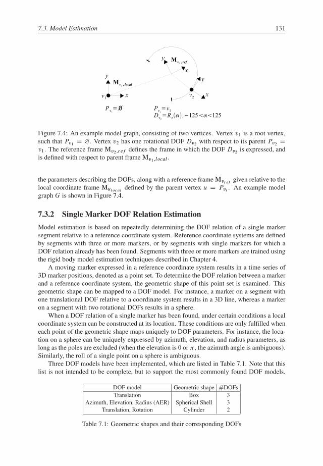
7.3. Model Estimation 131
Figure 7.4: An example model graph, consisting of two vertices. Vertex v1 is a root vertex,
such that Pv1D ∅. Vertex v2 has one rotational DOF Dv2
with respect to its parent Pv2D
v1. The reference frame Mv2;ref defines the frame in which the DOF Dv2is expressed, and
is defined with respect to parent frame Mv1;local .
the parameters describing the DOFs, along with a reference frame Mvr efgiven relative to the
local coordinate frame Mulocaldefined by the parent vertex u D Pvi
. An example model
graph G is shown in Figure 7.4.
7.3.2 Single Marker DOF Relation Estimation
Model estimation is based on repeatedly determining the DOF relation of a single marker
segment relative to a reference coordinate system. Reference coordinate systems are defined
by segments with three or more markers, or by segments with single markers for which a
DOF relation already has been found. Segments with three or more markers are trained using
the rigid body model estimation techniques described in Chapter 4.
A moving marker expressed in a reference coordinate system results in a time series of
3D marker positions, denoted as a point set. To determine the DOF relation between a marker
and a reference coordinate system, the geometric shape of this point set is examined. This
geometric shape can be mapped to a DOF model. For instance, a marker on a segment with
one translational DOF relative to a coordinate system results in a 3D line, whereas a marker
on a segment with two rotational DOFs results in a sphere.
When a DOF relation of a single marker has been found, under certain conditions a local
coordinate system can be constructed at its location. These conditions are only fulfilled when
each point of the geometric shape maps uniquely to DOF parameters. For instance, the loca-
tion on a sphere can be uniquely expressed by azimuth, elevation, and radius parameters, as
long as the poles are excluded (when the elevation is 0 or � , the azimuth angle is ambiguous).
Similarly, the roll of a single point on a sphere is ambiguous.
Three DOF models have been implemented, which are listed in Table 7.1. Note that this
list is not intended to be complete, but to support the most commonly found DOF models.
DOF model Geometric shape #DOFs
Translation Box 3
Azimuth, Elevation, Radius (AER) Spherical Shell 3
Translation, Rotation Cylinder 2
Table 7.1: Geometric shapes and their corresponding DOFs

132 7. Tracking and Model Estimation of Composite Interaction Devices
Figure 7.5: The fitting procedure.
Adding more DOF models does not change the techniques presented in this chapter.
Fitting routines are generally more efficient and more accurate for lower dimensions.
Therefore, the geometric shapes corresponding to each DOF model of Table 7.1 are divided
into simpler cases, and the corresponding geometric fitting routines are implemented. The
complete procedure of finding a single marker DOF relation relative to a coordinate system is
outlined in Figure 7.5. The fitting procedure is based on performing a Principal Component
Analysis to find the dimensionality of the point set. If the point set can be reduced to zero
dimensions, the data can be described by a single 3D point. In this case, a rigid relation
between two single marker segments is found. If the point set can be described by one
dimension, the data lies on a 3D line, such that the relation between two segments can be
described by one translational DOF. In case the point set can be described by two dimensions,
2D fitting routines are applied to find the geometric shape that best describes the data. If the
point set lies within a volume, 3D fitting routines are used. The fitting procedure and its
implementation is discussed in more detail in the following sections.
Dimensionality Reduction
The first step of the fitting procedure is to find the dimensionality of the point set, i.e., to
check if the point set can be described by a single 3D point, a line, a plane, or a volume. This
is accomplished by performing a Principal Component Analysis (PCA) [Jol02]. Principal
component analysis (PCA) is a powerful mathematical procedure that transforms a number
of (possibly) correlated variables into a smaller number of uncorrelated variables, which are
called principal components. The principal components are orthogonal, and are ordered de-
scending in terms of how much they account for the variability in the data. The PCA is a
popular technique to reduce the dimensionality of a data set or to detect structure in the re-
lationships between variables. It re-expresses a data set as a linear combination of its base
vectors. Consider a data set consisting of M measurements, where each measurement is rep-
resented by an L-dimensional vector vi , 0 � i < M . The PCA can be performed by the

7.3. Model Estimation 133
following steps:
1. Subtract the mean of each variable from each measurement
Ovi D vi �1
M
MX
jD1
vj (7.1)
2. Organize the resulting data set as an L �M matrix X
3. Compute the L �L covariance matrix C
C D 1
M � 1XX
T (7.2)
4. Calculate the eigenvectors V of C and sort by decreasing eigenvalue D.
CV D VD (7.3)
The eigenvectors define the set of principal components Ovi , whereas the eigenvalues corre-
spond to the principal values �i , such that the (centered) data set can be expressed by
�i Ovi (7.4)
The PCA can also be performed by calculating a Singular Value Decomposition (SVD) on
matrix X
X D U†VT (7.5)
where the columns of V are the principal components of X. The SVD serves as a one-step
function to perform PCA, without the need to explicitly compute the covariance matrix C.
Performing the PCA on a 3D point set results in three principal components. The first
component has the largest principal value, meaning it is a 3D vector in the direction that
represents the largest variability in the data. To test if the point set can be described by
one translational DOF, a line is constructed through the mean of the point set C and in the
direction D of the principal component with the largest principal value. This corresponds to
a least squares line approximation, where the orthogonal distance of the point set to the line
is minimized [Sha98]. The mean square error (MSE) of the orthogonal distances of the point
set to the line is used to determine if the point set can be accurately represented by a line
MSE DMX
iD1
jL � .pi � P /j2 (7.6)
where pi is a 3D point, P a point on the line, M the size of the point set, and L the normalized
line direction. If the MSE is below a specified threshold �, it is concluded that the point
set can be accurately described by a line. The threshold � depends on the measurement
noise introduced by the optical tracking system. If the geometric shape of the point set
is determined to be a line, a translational DOF has been found. The translation range is
determined by projecting the point set onto the line, using
.pi � P / �L (7.7)

134 7. Tracking and Model Estimation of Composite Interaction Devices
If the range is below �, the data is regarded as a single 3D point. In this case, the procedure
returns a zero DOF relation. Otherwise, the procedure returns one translational DOF and
its range. The reference frame Mref (see Section 7.3.1) is defined by the axes of the PCA
components, with the center in the mean of the point set.
To test if the data can be represented as a two dimensional set of points, a plane is fitted
to the data. The principal component with the smallest value is used as an estimate of the
plane’s normal vector N , with the mean of the point set as point in the plane. Analogous to
the line test, this corresponds to a least squares approximation, where the orthogonal distance
of the point set to the plane is minimized [Sha98]. The mean square error of the point set to
the plane is determined as
MSE DMX
iD1
.N � .pi � P //2 (7.8)
where N is the normal vector to the plane, and P is a point on the plane. If the MSE is below
�, the point set is regarded as planar. In this case, the point set is rotated such that the least
squares plane is the xy plane. This is accomplished by multiplying each point pi with the
matrix
Mplane D
0
B
B
B
@
1 � a2
cC1� ab
cC1�a 0
� abcC1
1 � b2
cC1�b 0
a b c 0
0 0 0 1
1
C
C
C
A
(7.9)
where (a, b, c) are the components or direction cosines of N . The procedure then performs
2D fitting routines on the transformed point set to find the most appropriate geometric shape.
In case the data cannot be accurately represented by one or two dimensional variables, the
data is considered to be volumetric.
2D Fitting Routines
If the point set lies in a plane, 2D fitting routines are performed. The point set is rotated such
that its least squares plane corresponds to the xy plane using Equation 7.9. Next, two 2D
fitting routines are performed: an annulus and a rectangle fit.
The rectangle fit is implemented as an optimization routine over one rotational variable
� around the z-axis, rotating the coordinate system in which the point set is expressed and
minimizing the rectangle defined by the x and y-range of the data. The downhill simplex
method is used for optimization (see also Chapter 4). During each function evaluation that
is performed by the simplex method, the x and y-range of the point set in the rotated frame
estimate Mrect D Rz.�/ is calculated. The area of the rectangle with ranges xr and yr is
minimized, such that the objective function J can be written as
J.�/ D xr yr (7.10)
where xr ; yr are functions from � .
To obtain an initial estimate of � , as needed by the simplex method, the principal com-
ponents are used as axes of the initial pose. These axes are rotated into the xy plane using
Equation 7.9. The PCA components generally give a good initial estimate of the pose of
the rectangle. Only when the width and height of the rectangle are identical, and assuming
uniformly distributed data, the obtained axes pass through the corners of the rectangle. This
situation is illustrated in Figure 7.6. In case the width and height of the rectangle differ, the

7.3. Model Estimation 135
−1 −0.5 0 0.5 1−1
−0.8
−0.6
−0.4
−0.2
0
0.2
0.4
0.6
0.8
1
x
y
(a)
−1.5 −1 −0.5 0 0.5 1 1.5−1
−0.8
−0.6
−0.4
−0.2
0
0.2
0.4
0.6
0.8
1
x
y
(b)
Figure 7.6: The PCA components of two uniform point sets. (a) The PCA components of a
uniform square point set give axes through its corners, (b) The PCA components of a uniform
rectangular point set give the desired axes.
Figure 7.7: An annulus with minimum and maximum radii r1 and r2, rotation range �r , and
center C .
axes obtained by the PCA are reasonably accurate. As is illustrated in the figure, the maxi-
mally allowed rotation of the initial estimate is 45 degrees, which defines the initial size of
the simplex.
The obtained solution Rz.�/ is rotated back from the xy plane using the transpose of
Mplane as defined in Equation 7.9, to form the reference frame Mref . The x and y ranges
are returned as DOFs.
The annulus fit is also implemented as a simplex optimization routine. An annulus is de-
fined as the region lying between two concentric circles (see Figure 7.7). It is fully described
by its center C , the inner radius r1, the outer radius r2, and the rotation range �r . This ge-
ometric shape corresponds to a rotational DOF, followed by a translational DOF. Using the
center of the annulus as optimization variable, the remaining parameters can be determined as
follows. The inner radius r1 and outer radius r2 are determined by calculating the minimum
and maximum distances of the point set to the center. The rotation range �r is determined by
expressing the point set in polar coordinates, and calculating the angle each point makes with
the x-axis. These angles are sorted to obtain �i ; i D 1; � � � ; N , such that �r can be calculated
as
�r D 2� �max.2� � �max C �min; maxi
.�iC1 � �i// (7.11)

136 7. Tracking and Model Estimation of Composite Interaction Devices
Figure 7.8: Obtaining the DOFs of a moving marker. First, a PCA is performed to obtain
the axes corresponding to the largest variability in the data. Next, the markers with minimal
and maximal x and y values are determined, and circle estimates are created through each
combination of three markers. An annulus fitting routines is used to obtain a final estimate of
the parameters of the geometric figure the marker describes. Finally, the annulus parameters
are mapped to a DOF model with one translation and one rotation.
The objective function J is defined as the area of this region, which is minimized as
J.C / DZ r2
r1
r
Z �2
�1
d�dr D 1
2.�2 � �1/.r2 � r1/2 D 1
2�r .r2 � r1/2 (7.12)
where r1; r2; �r are functions from C .
The complete procedure for fitting an annulus to motion data and mapping the parameters
of the annulus to a DOF model is outlined in Figure 7.8. First, the point set is expressed in the
coordinate system obtained from the principal component analysis. Next, an initial estimate
for the center C of the annulus is obtained. The minimal and maximal value of the x and
y components of each marker location is determined, yielding 4 coordinates. Three of these
coordinates should lie close to the circle with outer radius r2 (see Figure 7.8). Since a circle
can be defined by 3 non-collinear coordinates, each combination of 3 points (x1, y1), (x2,
y2), (x3, y3), is selected to calculate an estimate of the circle center (xc , yc).
The fitting routines are applied four times, using each combination of 3 points to provide
an initial estimate of the circle center C . The solution with the minimal area A is selected.
The parameters of the resulting annulus are mapped to a DOF model, with a rotational DOF
of range �r D �2 � �1, and a translational DOF in the range Œr1; r2�. The reference frame
Mref D MTplane
Rz.�m/T.C /, where Rz.˛/ represents a rotation matrix around the z-axis,
�m is the midway angle of the rotation range �r , and T.C / a translation matrix.

7.3. Model Estimation 137
3D Fitting Routines
The 3D fitting routines are executed when the point set lies within a volume. In this case, a
sphere, cylinder, and a box fit are performed.
The box fit is a trivial extension of the rectangle fit. It is implemented using the simplex
method, optimizing three rotation angles ˛, ˇ, that define the pose of the box.
Mbox D Rx.˛/Ry.ˇ/Rz. / D"
1 0 0
0 cos ˛ � sin ˛
0 sin ˛ cos ˛
#"
cos ˇ 0 sin ˇ
0 0 1
� sin ˇ 0 cos ˇ
#"
cos � sin 0
sin cos 0
0 0 1
#
(7.13)
During each function evaluation, the x, y, and z ranges of the point set expressed in Mbox
are determined. The objective function to be minimized is defined as the area of the resulting
volume xr yr zr . The three principal components are used as initial estimates to define the
axes of Mbox . The final solution gives the reference frame Mref .
Note that the minimum enclosing box and rectangle can also be found using the rotating
calipers method [Tou83, O’R85]. The rotating calipers method is based on the observation
that one side of a minimal rectangle must coincide with one edge of the convex hull of the
point set it contains. Therefore, only the orientations given by the edges of the convex hull
have to be considered. This can be extended to three dimensions to find the minimum enclos-
ing box. However, the PCA generally finds an accurate initial estimate of minimum enclosing
rectangles and boxes, such that the optimization procedures are efficient and provide a com-
mon framework for all fitting routines.
The cylinder and sphere fitting routines are standard least squares routines. The optimiza-
tion parameters of the cylinder fit are a point on the cylinder axis C , the direction of the axis
D, and the radius r . As discussed in [Sha98], the Levenberg-Marquardt algorithm can be
used as unconstrained optimization procedure to minimize the objective function
J.D; C; r/ DNX
iD1
.jD � .pi � C /j � r/2 (7.14)
A reasonable initial estimate for the cylinder axis can be obtained from the principal com-
ponents. The least squares fitting procedure is performed using each principal component as
an estimate of the cylinder axis, and the center of the data as point on the axis. The solution
that gives the lowest value of the objective function in Equation 7.14 is selected. The cylin-
der corresponds to a translational DOF, followed by a rotational DOF. The reference frame
Mref is given by the coordinate system with the z-axis aligned with the cylinder axis, and
the x-axis such that the angles that the data points make with the z-axis is symmetric around
zero. Similarly, the position of Mref is chosen such that the translations of the data points,
as obtained by projecting them onto the cylinder axis, are symmetric around zero.
The sphere fit is performed by optimization of its center C and its radius r . The objective
function to be minimized is given by
J.C; r/ DNX
iD1
.jpi � C j � r/2 (7.15)
Analogous to the annulus fit, the initial estimate for C and r are provided by expressing the
point set in the coordinate system defined by the principal components. Next, the minimum

138 7. Tracking and Model Estimation of Composite Interaction Devices
and maximum values of the x, y, and z components are determined, giving 6 coordinates.
Each combination of 4 points is used to calculate an estimate of C and r , which is used to
perform the least squares optimization. The solution with the lowest value of Equation 7.15
is selected. Next, the azimuth and elevation range in which the point set lies is optimized.
This is achieved by optimizing the elevation axis, expressed as two angles ˛; ˇ, to minimize
the objective function
J.˛; ˇ/ D .�2 � �1/.cos �1 � cos �2/r2 (7.16)
where �1; �2; �1; �2; r are functions from ˛; ˇ.
7.3.3 Skeleton Estimation
The fitting routines described in the previous section provide a method to determine the DOF
relation between a single marker and a reference coordinate system. By defining a local
coordinate system in a single marker location that moves according to its DOF, the DOF
relation between single markers can be determined. The basis of skeleton estimation is to
repeatedly execute the fitting techniques to find all possible DOF relations between each pair
of segments. These DOF relations are used to determine the ‘best’ skeleton structure of the
composite interaction device. This structure is optimized to contain those DOF relations
between segments that describe the structure most compactly. The skeleton structure is found
by calculating a minimum spanning tree (MST), where the fitting results of segment pairs are
compared to determine which DOF relation is to be considered more optimal than another.
The calculation of the MST is accomplished by an adaptation of Prim’s minimum span-
ning tree (MST) algorithm, as outlined in Algorithm 1. The procedure determines the model
graph G D .V; P; D; ‰/ as defined in Section 7.3.1.
The method works as follows. First, all data points are assigned to segments using the
marker identifiers obtained from frame-to-frame correspondence. Algorithm 1 then slowly
grows a minimum spanning tree that describes the hierarchical skeleton structure and DOF
relations of the segments of the device. It starts from a single segment and adds new DOF
relations that link the partial model tree to a new segment outside of the tree.
Algorithm 1 BUILD TREE.G.V; P; D; ‰//
Q V
for all u 2 Q do
Du NIL
end for
P0 NIL
while Q ¤ ; do
u EXTRACT MIN(Q)
for all v 2 Q do
d FIND DOF RELATION(v, u)
if SIMPLER DOF RELATION(d , Dv) then
Pv u
Dv d
end if
end for
end while
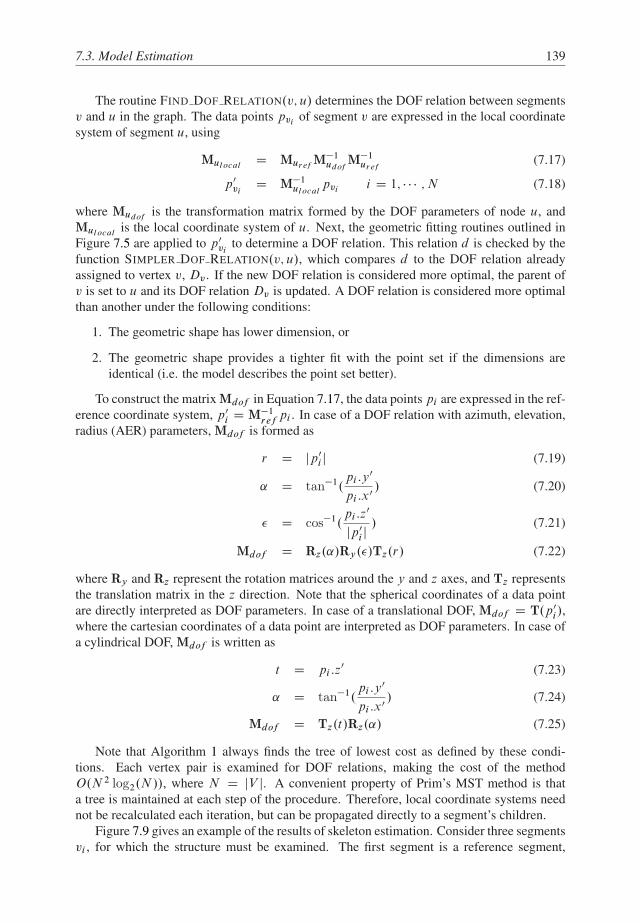
7.3. Model Estimation 139
The routine FIND DOF RELATION.v; u/ determines the DOF relation between segments
v and u in the graph. The data points pviof segment v are expressed in the local coordinate
system of segment u, using
MulocalD Mur ef
M�1udof
M�1ur ef
(7.17)
p0viD M
�1ulocal
pvii D 1; � � � ; N (7.18)
where Mudofis the transformation matrix formed by the DOF parameters of node u, and
Mulocalis the local coordinate system of u. Next, the geometric fitting routines outlined in
Figure 7.5 are applied to p0vi
to determine a DOF relation. This relation d is checked by the
function SIMPLER DOF RELATION.v; u/, which compares d to the DOF relation already
assigned to vertex v, Dv . If the new DOF relation is considered more optimal, the parent of
v is set to u and its DOF relation Dv is updated. A DOF relation is considered more optimal
than another under the following conditions:
1. The geometric shape has lower dimension, or
2. The geometric shape provides a tighter fit with the point set if the dimensions are
identical (i.e. the model describes the point set better).
To construct the matrix Mdof in Equation 7.17, the data points pi are expressed in the ref-
erence coordinate system, p0i D M
�1ref
pi . In case of a DOF relation with azimuth, elevation,
radius (AER) parameters, Mdof is formed as
r D jp0i j (7.19)
˛ D tan�1.pi :y
0
pi :x0/ (7.20)
� D cos�1.pi :z
0
jp0i j
/ (7.21)
Mdof D Rz.˛/Ry.�/Tz.r/ (7.22)
where Ry and Rz represent the rotation matrices around the y and z axes, and Tz represents
the translation matrix in the z direction. Note that the spherical coordinates of a data point
are directly interpreted as DOF parameters. In case of a translational DOF, Mdof D T.p0i/,
where the cartesian coordinates of a data point are interpreted as DOF parameters. In case of
a cylindrical DOF, Mdof is written as
t D pi :z0 (7.23)
˛ D tan�1.pi :y
0
pi :x0/ (7.24)
Mdof D Tz.t/Rz.˛/ (7.25)
Note that Algorithm 1 always finds the tree of lowest cost as defined by these condi-
tions. Each vertex pair is examined for DOF relations, making the cost of the method
O.N 2 log2.N //, where N D jV j. A convenient property of Prim’s MST method is that
a tree is maintained at each step of the procedure. Therefore, local coordinate systems need
not be recalculated each iteration, but can be propagated directly to a segment’s children.
Figure 7.9 gives an example of the results of skeleton estimation. Consider three segments
vi , for which the structure must be examined. The first segment is a reference segment,

140 7. Tracking and Model Estimation of Composite Interaction Devices
Figure 7.9: An example of skeleton estimation. The model consists of three segments, where
segment v1 is a reference segment. Segment v2 has one rotational DOF Dv2with respect
to its parent Pv2D v1. Segment v3 has one translational DOF Dv3
relative to its parent
Pv3D v2.
for which a full coordinate system has been obtained by the rigid body model estimation
techniques. Skeleton estimation proceeds by examining all (node, parent) relations (v2, v1),
(v3, v1), (v2, v3), and (v3, v2). The resulting structure is (v2, v1), (v3, v2), such that v2 has
one rotational DOF relative to v1 and v3 has one translational DOF relative to v2. Other
structures are suboptimal. Consider for instance a structure that includes the relation (v3; v1/.
Expressing the point set of segment v3 in Mv1;local results in a complex two-dimensional
figure, that cannot be expressed in one variable. In contrast, expressing the point set of v2 in
Mv1;local results in a circle arc, which can be represented by one rotational DOF.
7.3.4 Handling Noise
The model estimation techniques presented in this chapter are sensitive to noise and outliers
in the data. To remove outliers from the data, a simple clustering technique is used. Since
each marker trajectory is a time series, the position of a marker at time t is close to the
position at time t C �t , where 1�t
represents the frame rate at which data is recorded. As a
result, data points that are further than a certain threshold distance from the rest of the time
series are removed. Since during model estimation motion is slow and smooth, this threshold
can be chosen small.
An alternative approach would be to use a RANSAC [FB81] algorithm. RANSAC chooses
random sets of points to which the fitting methods are applied, until a fit metric is within a
given tolerance. This has the advantage of making the model estimation method very robust
against noise and outliers. The disadvantage is that model estimation takes longer.
Other techniques to make the model estimation techniques more robust are to apply filter-
ing and prediction techniques to compensate for noise and latency (see Chapter 6). Another

7.4. Model-based Object Tracking 141
approach would be to use weighted fitting routines, where data points are given a measure
of importance based on various metrics, e.g. blob size, distance from the epipolar lines, and
local density.
7.4 Model-based Object Tracking
Given labeled 3D marker locations, model-based object tracking proceeds in three steps.
� Rigid body tracking
The segments that consist of three or more markers are identified. These segments
define the initial reference frames used to identify single marker segments. They are
tracked using the rigid body tracking techniques described in Chapter 4.
� Single marker segment tracking
The skeleton structure and DOF model are used to identify single marker segments.
� Occlusion handling
The situation where the parent of a segment is lost due to occlusion is dealt with. In
these cases, the children of the lost segment cannot be found by using the DOF relations
in the skeleton structure.
7.4.1 Single Marker Segment Tracking
The goal of tracking the single markers segments is to determine the values of their degrees of
freedom with respect to their parents. These DOFs can be coupled to application parameters,
which a user needs to manipulate in order to perform a complex interaction task.
The DOFs of each segment are determined by using the reference coordinate systems
obtained from rigid body tracking and the model information. The model defines the skeleton
structure and the DOF relations and ranges of the single marker segments. An exhaustive
search is performed that matches markers to model segments, and prunes the search space
using a backtracking approach. The resulting procedure is outlined in Algorithm 2.
The procedure TEST DOF.S; p/ is called for each unidentified marker p and each seg-
ment S for which a reference coordinate system has been found. A stack � is maintained,
Algorithm 2 TEST DOF(S; p)
�:PUSH(S; p)
if DOFMATCH(S; p) then
S:m p
UPDATEBEST()
for all S 2 CHILDREN(S ) do
for all p 2 P do
TEST DOF(S; p)
end for
end for
else
�:POP()
end if

142 7. Tracking and Model Estimation of Composite Interaction Devices
which holds the matches between segments and markers. When the procedure is called, the
stack is updated, and DOFMATCH.S; p/ is called to check if the current point can be ex-
pressed by the DOF model of segment S . The point p is expressed in the reference frame
Mref of S , and its DOF parameters are calculated according to the model. If the parame-
ters are within the ranges of the DOF parameters in the model, the best match is updated by
calling UPDATEBEST./, and the child segments of S are examined. If there is no match, the
algorithm backtracks by popping the stack � . Note that Algorithm 2 is a simple extension of
a depth first search to include a backtracking step.
The procedure finds a maximum length match between markers and model segments. It
exploits the hierarchy in the model for efficient DOF testing. Since it maintains a tree, the lo-
cal coordinate systems of identified segments can be stored and used in subsequent segments.
The model allows for information propagation during tracking. As relations between mark-
ers and reference frames are determined, this information is used to construct new reference
frames to identify new segments. However, when a segment is lost, the procedure fails to
find its child segments. In the next section, the techniques used to make the tracker robust to
occluding segments are discussed.
7.4.2 Occlusion Handling
The previous sections have described methods to track segments with three or more points,
and how this information is used to construct reference coordinate systems and to identify
segments with single markers. The techniques for tracking three or more points require suf-
ficient points to unambiguously construct a coordinate system, but do not require all points
of the segment to be visible. However, when a single marker segment is occluded, all its
child segments cannot be identified. The DOFs of these segments are defined relative to the
local coordinate system of the occluded segment. To address this problem, the DOF relations
between all segments are stored in the model, next to the DOF relations that are part of the
skeleton structure. The skeleton relations are used for the tracking procedure described in
Section 7.4.1. In case some segments are determined to be occluded and unidentified mark-
ers are present after this procedure, the remaining relations are used to identify single marker
segments relative to other parent segments.
In general, only the 3D location of segments with an occluded parent can be determined.
Only when a parent segment is completely redundant, i.e., when an unambiguous relation of
its child segments with other parents was correctly found, the DOF parameters of the child
segments and of the lost parent segment can be determined. As such, extra redundancy can
be introduced to the interaction device. The advantage is that the device is better suited to
handle partial occlusion.
7.5 Results and Discussion
The model-based optical tracking and automatic model estimation techniques have been im-
plemented and evaluated in the PSS. For the following tests, a two-camera setup was used.
7.5.1 Model Estimation
Figures 7.10 and 7.11 show the results of model estimation for two composite interaction
devices. The figures depict the devices, along with the model points as determined by the

7.5. Results and Discussion 143
Figure 7.10: Model estimation results of a composite interaction device. At the top, a crane
is depicted, along with the model points. At the bottom left, the complete model is illustrated
with the skeleton structure, reference coordinate systems, model points, and DOF relations
and ranges. The bottom right shows the complete model including local coordinate systems
at the marker locations.

144 7. Tracking and Model Estimation of Composite Interaction Devices
Figure 7.11: Model estimation results of a composite interaction device. At the top, a finger
is depicted, along with the model points. At the bottom left, the complete model is illustrated
with the skeleton structure, reference coordinate systems, model points, and DOF relations
and ranges. The bottom right shows the complete model including local coordinate systems
at the marker locations.

7.5. Results and Discussion 145
Crane Finger
seg. model param range model param range
a -90.3 90.3 a -19.3 19.3
1 AER e 90 90 AER e 34.8 115.0
r 2.46 2.58 r 3.55 3.55
a -40.6 40.6 a -2.4 2.4
2 AER e 90 90 AER e 4.6 108.5
r 3.98 4.16 r 2.34 2.34
x -1.29 1.29 a -1.56 1.56
3 Trans y 0 0 AER e 63.6 129.6
z 0 0 r 1.43 1.43
Table 7.2: DOF ranges of the device segments of Figures 7.10 and 7.11, where rotational
DOFs are given in degrees, and translational DOFs in cm.
automatic model estimation procedure. The lower parts of the figures show the complete
models, including reference coordinate systems and DOF relations and ranges, and the mod-
els with the local coordinate systems at the marker locations, as defined by the DOF relations.
Table 7.2 lists the relevant DOF parameters corresponding to the models in Figure 7.10. Both
devices were moved in front of the cameras over a period of about one minute (3397 frames
for the crane, and 3162 frames for the hand). The developer should take care to sweep through
the DOF ranges, so that the system has enough data to recognize the underlying geometric
shapes. After the developer has shown the system all DOFs in the device, skeleton estimation
is performed. This procedure took less than 30 seconds for the examples in Figures 7.10 and
7.11. The DOF parameters listed in Table 7.2 were verified by hand, and by applying the
obtained model in the tracking system.
Note that these devices represent simple examples, illustrating some of the DOFs the sys-
tem can handle. For instance, an assumption of the finger example is that the thumb is not
moved, so that the reference frame is kept rigid. In a practical situation, one could attach a
rigid structure to the hand or glove. In Chapter 8, the model estimation and tracking tech-
niques for composite interaction devices are applied in a real world scenario. A configurable
interaction device is developed and applied in various VR applications.
The 3D marker locations that are reported by the tracking system of the PSS contain mea-
surement noise, which is included in the model estimation procedure. Since this noise is en-
countered in practice during tracking, it is advantageous that this noise is modeled. However,
noise is propagated as more segments are connected during the model estimation procedure.
Obtained DOF relations between single markers and reference coordinate systems are used to
construct new coordinate systems. A subsequent marker expressed in this coordinate system
contains a combination of its own noise and the noise in the coordinate system. As an exam-
ple, the radius range of the first single marker segment of the crane in Figure 7.10 is about
1.1 mm (which ideally should be 0). Its child segment has a radius range of 1.8 mm, which
is a combination of its own noise and the noise of its parent segment. Clearly, long chains
of segments are more difficult to train, as the tolerances of the fitting routines would have to
be set to prohibitively high values. However, the noise can be reduced by using a weighted
fitting strategy, such that more trusted data is more important. For instance, a local density
estimate of each data point can be used as a weight factor.
Another possibility to increase the accuracy of the model is to use more cameras. A very
minimal setup with only two cameras was used, where the noise in a single 3D point was

146 7. Tracking and Model Estimation of Composite Interaction Devices
-100
-50
0
50
100
0 500 1000 1500 2000
an
gle
(d
eg
)
frame
Segment 1Segment 2
-0.015
-0.01
-0.005
0
0.005
0.01
0.015
0 500 1000 1500 2000
tra
nsla
tio
n (
m)
frame
Segment 3
Figure 7.12: The DOFs of the crane model, as determined by the tracking system during a
39-second motion data set. (Top) The rotational DOFs of the crane’s base and arm. (Bottom)
The translational DOF of the crane’s arm extension.
determined to have a maximum value of about 2 mm. More cameras or larger markers would
provide more accurate 3D point measurements. One could also use more markers on a single
segment higher up a chain. Each segment for which a full reference frame can be determined
effectively resets the noise propagation in a chain.
Note that this system only finds DOF relations between single marker segments and a
reference coordinate system. When an interaction device contains multiple segments with
three or more points, the DOF relation between two coordinate systems also needs to be
determined. To support DOF relations between coordinate systems, the work of Hornung
et al. [HSDK05] could easily be incorporated, extending their approach to provide a higher
level DOF description. The skeleton estimation and tracking procedures would remain the
same.
The motion data sets to obtain the models of Figures 7.10 and 7.11 were both about a
minute in length. Model estimation completes in less than a minute. The time required
for calculating a model depends on the structure of the device, the complexity of the fitting
routines, and the complexity of the skeleton estimation procedure, which is O.N 2 log2.N //
with N the number of segments. Clearly, for larger data sets computation time increases
rapidly. However, the model estimation procedure is a post processing procedure, which is
fully automated.
7.5.2 Model-based Object Tracking
The model of the crane as acquired from the model estimation procedure (see Figure 7.10)
was used as input to the model-based tracking system. Figure 7.12 depicts the DOFs of
each segment for a data sequence of 2360 frames, which is about 39 seconds. In this se-
quence, each segment was manipulated with varying speeds. The tracking system identified
all segments and their DOFs correctly in 97.16% of the data sequence. The figure shows the
rotational DOF of the base of the crane and the rotational DOF of the arm. On the right, the
translational DOF of the arm’s extension is shown. The system maintains a frame rate of 60
Hz throughout the tracking sequence, which is constrained by the speed of the cameras.
A problem may occur during tracking when invalid markers, or markers from other de-
vices, come within the range of a DOF relation between two segments. Since the tracker tries
to maximize the number of matches between markers and segments, the system often rejects
these stray markers. However, if a stray marker comes within the DOF range of a segment

7.6. Conclusion 147
without children, it is uncertain which marker is the correct one. In these cases, the tracking
system could use history information to determine the best match.
7.6 Conclusion
In this chapter, a model-based optical tracking and automatic model estimation system was
presented. The system supports composite interaction devices, which consist of several seg-
ments connected in a tree structure. Segments can have combinations of translational and
rotational degrees of freedom with respect to a parent segment. The system requires only one
segment to contain three or more markers, such that a full coordinate system can be deter-
mined and the tracking system can be kept fast and efficient. Other segments may contain
only one marker. This allows for small interaction devices, without the need for large num-
bers of markers on each moving segment. Moreover, when larger numbers of markers are
used, the model automatically includes this extra redundancy, allowing for more occlusion
during tracking.
The model provides a high level DOF description between segments, along with the
ranges of these DOFs and the skeleton structure. No pre-defined models are required. The
tracking system uses the model estimate to recognize the device in a backtracking approach.
The tracking method supports partial occlusions.
Model estimation is based on estimating the DOF relation between a marker and a coordi-
nate system. When such a relation has been found, the system determines a local coordinate
system in the marker according to the DOFs. However, noise may get propagated throughout
a branch of connected segments. More research can be done to investigate noise reduction
techniques. For instance, a local density estimate could be used as an importance measure of
a data sample.

148 7. Tracking and Model Estimation of Composite Interaction Devices

Chapter 8
A Configurable Interaction Device
In Chapters 3 and 4, techniques were developed and evaluated for optical tracking and au-
tomatic model estimation of rigid interaction devices. In Chapter 6 filtering and prediction
techniques were analyzed, which can be used to reduce noise and latency problems. The
developed tracking techniques were extended in Chapter 7 to handle composite interaction
devices. In this chapter, all these techniques are combined in an optically tracked config-
urable interaction device. The aim of the device is to allow an interface developer to rapidly
construct new devices, of which the spatial structure can match the structure of the task at
hand. The device is tested in a number of application scenarios.
8.1 Introduction
Interaction in a virtual environment is often a complicated task. Designing effective inter-
action techniques is especially difficult when a user has to manipulate many parameters to
complete a task. There have been various approaches to designing input devices for such
high dimensional input tasks. One approach is to use a device with a relatively small number
of degrees of freedom (DOFs) that can be put into different modes, for instance by using extra
buttons or menu selections. Such mode switching may interrupt the task flow and present an
extra cognitive load on the user [JS92]. Another option is to use multiple devices and assign
different subtasks to each of them. In this case, mode switching is implicit in the selection
of a device, and may present the same interruption of task flow. One could also construct
a single device specific for a particular application or interaction task. This way, a user has
direct control over all required DOFs. However, constructing a new device from scratch for
each interaction task is inefficient and impractical.
An approach to relieve these limitations would be to construct flexible interfaces, which
can be reconfigured for specific interaction tasks. One way to achieve this is to create in-
terfaces that can easily be changed in software, for instance by using 2D widget interfaces
attached to handheld props [CW99, KL04].
In this chapter, another approach is explored: the development and application of a con-
figurable input device, which can easily be configured specifically for a required interaction
task. The aim of the device is to meet the objectives as defined in Chapter 1:
� A user should be able to manipulate a large number of application parameters with a
single, compact device.
� A developer should be able to structure the device such that it reflects the parameters
of the interaction task at hand.
� A developer should be able to rapidly develop new interaction techniques and test new
149

150 8. A Configurable Interaction Device
Figure 8.1: An example device configuration with three actuators.
configurations.
� The device should be optically tracked, resulting in a compact, light, wireless, low-cost,
and unobtrusive interaction device.
� Two-handed interaction and proprioception should be exploited.
The developed configurable interaction device (CID) is based on two components: the
base object and the actuators. Each configuration of CID consists of a base object, which
defines a (six DOF) frame of reference. The base object has a number of connection points,
to which actuators can be attached. Actuators define interaction relative to the base object.
They can have various combinations of translational and rotational degrees of freedom. For
instance, an actuator can be a slider, having one translational DOF, or a joystick, having
two rotational DOFs. An actuator may consist of several linked segments, incorporating
multiple joints. Interaction is performed by positioning and orienting the base object and by
manipulating the actuators.
An example configuration of CID is shown in Figure 8.1. The base object is a box,
to which three actuators are attached. The actuator on the top has two rotational DOFs,
corresponding to a joystick. The left actuator has one translational DOF, while the right
actuator has one rotational and one translational DOF.
CID is optically tracked. This allows CID to be low-cost, compact, light weight, wireless,
and unobtrusive. The tracking system is described in Chapter 7. It needs to identify at least
three markers on the base object to be able to unambiguously determine a frame of reference,
whereas actuators can have as little as one marker. This results in configurations that are
small enough for comfortable interaction. The system can automatically obtain a hierarchical
model of a new configuration of CID by the model estimation procedure described in Chap-
ter 7. During this procedure, a developer simply moves the device in front of the cameras,
manipulating each actuator such that the system can determine the DOFs and DOF ranges of
each actuator.
The configurable interaction device was tested in three application scenarios. The first is

8.2. Related Work 151
a modeling application, which enables a user to quickly design new object shapes by manipu-
lating a set of control points. The second is a scientific visualization application, used for the
manipulation and exploration of a volume rendering of a human head. The third application
enables a user to create animations of a 3D virtual representation of a human skeleton.
This chapter is organized as follows. In Section 8.2, related work is reviewed. Section 8.3
describes the configurable interaction device in detail. In Section 8.5, the flexibility of CID
is illustrated using three device configurations in different application scenarios. Section 8.6
provides a discussion of the results. Finally, in Section 8.7 conclusions are given.
8.2 Related Work
Relatively little work has been done on interaction devices that enable a user to manipulate
a large number of degrees of freedom in a single device. Most previous work on devices
for complex interaction tasks uses multiple props. For instance, Hinckley et al. [HPGK94]
proposed two handed interaction for neurosurgical visualization using several props. Balakr-
ishnan et al. [BFKS99] presented a single, application specific device for curve and surface
manipulation. It is based on a bend and twist sensitive strip.
Ayers et al. [AZ96] presented a rapid prototyping system for physical interaction devices.
The system allows quick assembly of interaction hardware based on snapping Lego R parts
together. However, the system is limited to three types of sensors. Fitzmaurice et al. [FIB95]
presented a software and hardware framework for graspable user interfaces. The framework
allows for rapid development of interfaces for complex interaction tasks.
Various researchers have proposed the use of 2D widget interfaces attached to handheld
props [CW99, KL04]. Subramanian et al. [SAM03] evaluated the use of hybrid 2D and 3D
interfaces. An experiment was conducted that requires users to navigate an intersection plane
through a solid 3D model, in order to locate a disc hidden inside the body of the model. They
found that the combination of a 3D and a 2D prop, along with the possibility of constraining
the DOFs, allowed users to complete the task faster than using only a 2D or 3D interface.
The configurable interaction device presented in this chapter shares ideas with the Cubic
Mouse, which was presented by Frohlich et al. [FP00]. The Cubic Mouse is a handheld de-
vice, designed for complex interaction tasks. It allows for direct manipulation of a relatively
large number of parameters. The device is depicted in Figure 1.3(b). It consists of a cubic
base, with three orthogonal rods passing through it. Virtual objects can be translated and ro-
tated relative to the pose of the cube by manipulating the rods. It is mostly used for scientific
data visualization, where the cube controls the pose of a 3D model, and the rods are used to
move slicing planes through the data set using position control techniques.
Simon et al. [SF03] introduced the YoYo, a handheld interaction device that combines
elastic force input and isotonic input. The device is depicted in Figure 1.3(c). It consists of
a cylindric base, with two rings on each side that can be moved relative to the base. The
rings are used as elastic six DOF force sensors. The device enables a user to directly control
a coordinate system using the cylindric base, and two additional coordinate systems using
elastic force input.
This chapter complements previous work by introducing a configurable interaction de-
vice, rather than a fixed device suited for a specific type of application. A developer can
rapidly design and evaluate new interaction devices. Moreover, the device allows for a direct
relation between the structure of the device and the parameters of the interaction task.
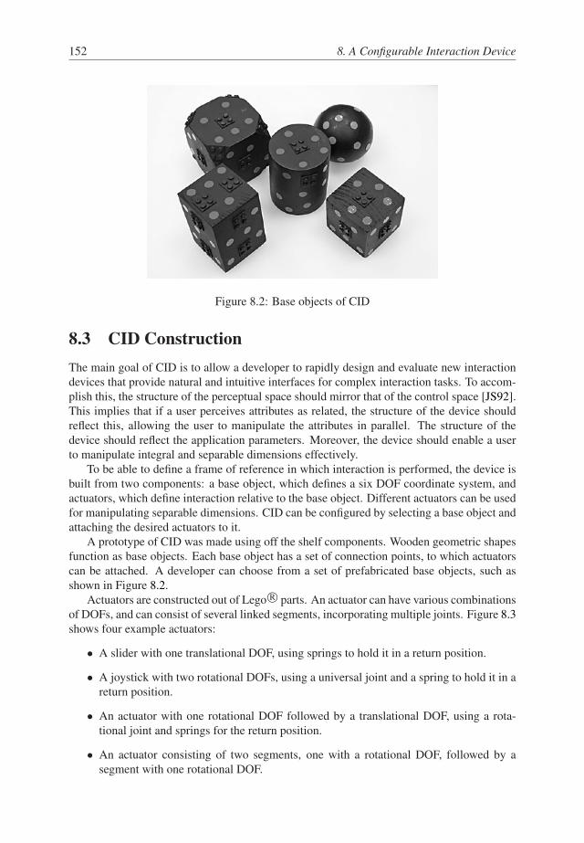
152 8. A Configurable Interaction Device
Figure 8.2: Base objects of CID
8.3 CID Construction
The main goal of CID is to allow a developer to rapidly design and evaluate new interaction
devices that provide natural and intuitive interfaces for complex interaction tasks. To accom-
plish this, the structure of the perceptual space should mirror that of the control space [JS92].
This implies that if a user perceives attributes as related, the structure of the device should
reflect this, allowing the user to manipulate the attributes in parallel. The structure of the
device should reflect the application parameters. Moreover, the device should enable a user
to manipulate integral and separable dimensions effectively.
To be able to define a frame of reference in which interaction is performed, the device is
built from two components: a base object, which defines a six DOF coordinate system, and
actuators, which define interaction relative to the base object. Different actuators can be used
for manipulating separable dimensions. CID can be configured by selecting a base object and
attaching the desired actuators to it.
A prototype of CID was made using off the shelf components. Wooden geometric shapes
function as base objects. Each base object has a set of connection points, to which actuators
can be attached. A developer can choose from a set of prefabricated base objects, such as
shown in Figure 8.2.
Actuators are constructed out of Lego R parts. An actuator can have various combinations
of DOFs, and can consist of several linked segments, incorporating multiple joints. Figure 8.3
shows four example actuators:
� A slider with one translational DOF, using springs to hold it in a return position.
� A joystick with two rotational DOFs, using a universal joint and a spring to hold it in a
return position.
� An actuator with one rotational DOF followed by a translational DOF, using a rota-
tional joint and springs for the return position.
� An actuator consisting of two segments, one with a rotational DOF, followed by a
segment with one rotational DOF.

8.4. Parameter Mapping 153
Figure 8.3: Four examples of actuators: a slider with one translational DOF, a joystick with
two rotational DOFs, an actuator with one translational and one rotational DOF, and a multi-
segment actuator with two rotational DOFs followed by an additional rotational DOF.
CID is tracked using a model-based optical tracking system. The tracker needs to deter-
mine the pose of the base object and the DOF values of the actuators, and send them to the
application. The system requires that a base object contains three or more (non-collinear)
markers, such that a frame of reference can be determined. Figure 8.2 shows these markers
as orange circles on the wooden objects. Actuators can have one or more markers per seg-
ment, which are shown in Figure 8.3 as silver spheres. Since the tracking system only needs
a single marker for an actuator, CID can be kept compact.
8.4 Parameter Mapping
The tracking system developed in Chapter 7 sends the pose of the base object and the de-
grees of freedom of each actuator directly to the virtual reality application. As a result, the
mapping between device DOFs and application parameters has to be hard coded into an ap-
plication. Consequently, during the development and evaluation of different interaction tech-
niques, the application needs to be repeatedly adjusted. This makes the development cycle a
time-consuming and inefficient process.
The flexibility of CID can be improved by adding a step between the tracker and the
application, which maps device DOFs to one-dimensional application variables. This way, a

154 8. A Configurable Interaction Device
Figure 8.4: Generic mapping of device DOFs to application parameters.
developer is able to adjust various factors that influence the interaction with an actuator, such
as its sensitivity, threshold, offset, and filtering parameters, and whether it is position or rate
controlled. The effects of changes in the mappings on the interaction can be directly studied
in the application.
A generic mapping is introduced between the application and tracker, as illustrated in Fig-
ure 8.4. The system consists of four components.
� A map daemon continuously monitors the tracker and application, and maps incoming
tracker events to application variables. The tracker and application register at the map
daemon at startup.
� A tracker transmits a list of device parameters to the map daemon upon registration.
The parameters describe the type, the range, and the name of each DOF.
� An application sends a list of variables to the map daemon that can be manipulated by
user interaction. The map daemon then continuously observes the tracker events, maps
them to application variables, and sends these on to the application.
� A map editor is used to create connections between application variables and device
DOFs.
An implementation of the map editor is depicted in Figure 8.5. The figure shows the
mapping that was used for the scientific visualization application described in Section 8.5.2.
The pose of the base object is considered a special case, and can only be connected to an
application variable that represents a 4 � 4 transformation matrix. All other mappings are
used to transform the value of a device DOF dk at time k to an application variable pk . A
mapping is described by the following parameters:
� Gaussian filter
A Gaussian filter with the specified odd-sized kernel size is applied to the device DOF
dk , resulting in the estimated device DOF Odk . The filter is described in Chapter 6 by
Equations 6.11 and 6.12.
� Input Parameter
The input parameter defines how the estimated DOF value Odk is used in the mapping
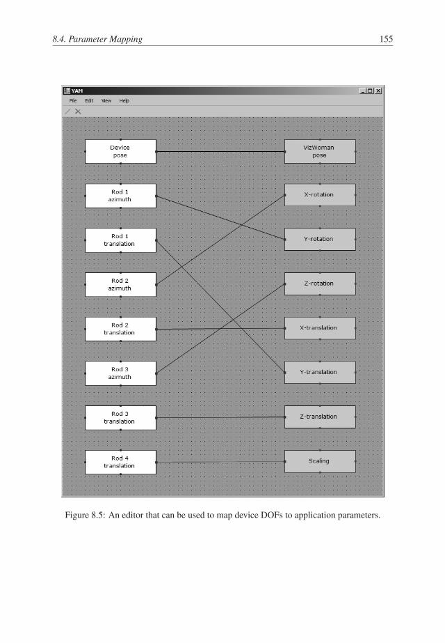
8.4. Parameter Mapping 155
Figure 8.5: An editor that can be used to map device DOFs to application parameters.

156 8. A Configurable Interaction Device
function. The input parameter can be set directly to the DOF value Odk , or to the differ-
ence between the current and last DOF estimates Odk and Odk�1. In case the DOF is a
rotation, the angular difference is used. As such, the input parameter vk is defined by
vk D
8
ˆ
<
ˆ
:
Odk DOF valueOdk � Odk�1 positional DOF difference
‚. Odk � Odk�1/ angular DOF difference
where the function ‚.��/ is used to normalize the angular difference to the range
Œ�pi; pi/:
‚.��/ D
8
<
:
�� �� � �� < �
�� C 2� �� < ��
�� � 2� �� � �
� Target range
A scaling function S.v; r/ is defined as a linear mapping of the input range v D Œx1; x2�
to the target range r D Œr1; r2�. The function is applied to the input vk , resulting in a
scaled value sk which is given by
sk D S.vk ; r/ D .vk � x1/r2 � r1
x2 � x1
C r1 (8.1)
� Threshold
A threshold function T .v; �/ is defined that returns v if jvj > � and v otherwise. The
function is applied to the scaled value sk , resulting in
tk D T .sk ; �/ D�
0 jsk j � �
sk jsk j > �
Changes in a (scaled) DOF that fall below � are not considered as input changes. As
such, a dead zone is introduced in which manipulations of the device DOFs do not
generate application events. This can be used to reduce unintended operations within
the application due to noise in the DOF estimates.
� Quantization
A continuous value can be mapped to a discrete range by specifying a quantization
value q. For instance, a rotation between 0 and 360 degrees can be mapped to a discrete
interval of integers in the range of 0 to 10 by setting the quantization value to 36. A
quantization function Q.v; q/ is used to round the value tk to its nearest discrete value,
using
qk D Q.tk ; q/ D qb tk C 0:5
qc (8.2)
Alternatively, the quantization function can be set to round to the lower or upper dis-
crete value.
� Control type
This parameter describes the type of control mechanism by which an object’s position
or orientation is changed. The choices are direct or incremental control. Generally,
direct is used for position control scenarios, which refers to the case where a user can
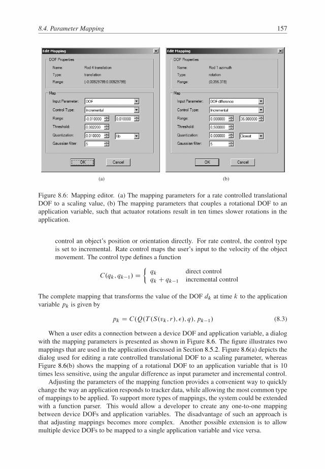
8.4. Parameter Mapping 157
(a) (b)
Figure 8.6: Mapping editor. (a) The mapping parameters for a rate controlled translational
DOF to a scaling value, (b) The mapping parameters that couples a rotational DOF to an
application variable, such that actuator rotations result in ten times slower rotations in the
application.
control an object’s position or orientation directly. For rate control, the control type
is set to incremental. Rate control maps the user’s input to the velocity of the object
movement. The control type defines a function
C.qk ; qk�1/ D�
qk direct control
qk C qk�1 incremental control
The complete mapping that transforms the value of the DOF dk at time k to the application
variable pk is given by
pk D C.Q.T .S.vk ; r/; �/; q/; pk�1/ (8.3)
When a user edits a connection between a device DOF and application variable, a dialog
with the mapping parameters is presented as shown in Figure 8.6. The figure illustrates two
mappings that are used in the application discussed in Section 8.5.2. Figure 8.6(a) depicts the
dialog used for editing a rate controlled translational DOF to a scaling parameter, whereas
Figure 8.6(b) shows the mapping of a rotational DOF to an application variable that is 10
times less sensitive, using the angular difference as input parameter and incremental control.
Adjusting the parameters of the mapping function provides a convenient way to quickly
change the way an application responds to tracker data, while allowing the most common type
of mappings to be applied. To support more types of mappings, the system could be extended
with a function parser. This would allow a developer to create any one-to-one mapping
between device DOFs and application variables. The disadvantage of such an approach is
that adjusting mappings becomes more complex. Another possible extension is to allow
multiple device DOFs to be mapped to a single application variable and vice versa.

158 8. A Configurable Interaction Device
8.5 Applications
CID was evaluated in the PSS, using a tracking setup with four cameras. The device was
tested in three application scenarios, each requiring a different configuration. The first is
a simple modeling application, which enables a user to create surfaces of revolution. The
second is a scientific visualization application, which is used for data exploration and manip-
ulation of a volume rendering of a CT scan. The third application is an animation package. In
this application, CID is configured to resemble a human body. By manipulating the actuators
of the configuration, the limbs of a model of a human skeleton can be moved into a desired
pose. A smooth animation can be created by defining key frames that describe a collection of
skeleton poses.
In all applications, the base object is used to define a coordinate system, which is coupled
to a virtual object or scene. This basically enables a user to hold an object in his non-dominant
hand, while the dominant hand performs the interaction on the object by manipulating the
actuators. This type of two-handed interaction exploits proprioception [Gui87].
8.5.1 Modeling
The first application is a modeling application, which allows a user to create surfaces of
revolution (see Figure 8.7(a)). A surface of revolution is a surface generated by rotating a
two-dimensional curve about an axis. The curve is described by a number of control points.
The shape of the object can be altered by selecting and moving control points.
CID is configured as illustrated in Figure 8.7(b). The base object is a 55�55�55 mm
cube, which defines the coordinate system of the surface of revolution, allowing a user to
hold the surface of revolution in his hands.
At the top of the cube, an actuator is attached which has one translational DOF. This
slider is used to select the active control point. Pushing and pulling the slider selects the next
or previous control point. The slider can be pushed and pulled relative to the cube over 1.9
cm. To ensure no unintended selections occur, a dead zone was defined in which the slider is
inactive. The threshold value for this dead zone was set to 3 mm.
At the right side of the cube, an actuator with one rotational DOF followed by a trans-
lational DOF is attached. The rotational DOF of this actuator allows the user to move the
control point up and down with respect to the object’s axis, whereas the translational DOF
is used to move the control point from and towards the axis. The actuator is held in a re-
turn position by springs. The angular range is 116 degrees, whereas the translation range
is 1.3 cm. The interaction on the control point is rate-controlled, meaning that the speed of
movement of the control point depends on the deviation of the actuator from its reference po-
sition. Analogous to the actuator used for control point selection, a dead zone was included
for robustness.
Figure 8.7(c) depicts the model obtained by the device training procedure. The model
shows the 3D marker locations on the base object, along with the DOFs and DOF ranges of
the actuators.
8.5.2 Manipulation and Data Exploration
A scientific visualization application was created, enabling data exploration and manipula-
tion. A user is presented with a volume rendering of a Computed Tomography (CT) scan of
a human head (see Figure 8.8(a)). Three orthogonal slicing planes can be manipulated to cut

8.5. Applications 159
(a) (b)
(c)
Figure 8.7: (a) A modeling application. (b) CID’s configuration, consisting of a cube and two
actuators controlling the shape of the virtual model. (c) The model of the configuration, as
acquired by the device training procedure.
through the data set along the main axes. Slicing a data set is a basic and frequently used task
in scientific visualization for data exploration. Additionally, the user is able to zoom in/out
of the data set, and the data set can be rotated with respect to the slicing planes.
CID is configured as depicted in Figure 8.8(b). The base object is a 7�7�7 cm truncated
cube. This base object is coupled to the virtual data set of the CT scan, such that the data set
can be viewed from every angle.
Three sides of the interaction device are equipped with actuators having one rotational
DOF and one translational DOF along the rotation axis. The translational components allow
the user to move the slicing planes along the principal axes that are defined by the truncated
cube. The rotational component allows for rotation of the data set around these principal
axes.
The degree to which a user is able to bring a data set closer to him for closer inspection is
limited in the PSS. Therefore, an extra actuator with one translational DOF is attached to one

160 8. A Configurable Interaction Device
(a) (b)
(c)
Figure 8.8: (a) A scientific visualization application for manipulation and data exploration.
(b) CID’s configuration, consisting of a truncated cube and 4 actuators. Three actuators
control three orthogonal slicing planes, whereas the one at the corner controls the zoom factor.
(c) The model of the configuration, as acquired by the device training procedure.
of the corners of the truncated cube to allow for scaling. Pulling the slider out scales the data
set up, while pushing the slider in scales it down. The mapping parameters of this actuator
are illustrated in Figure 8.6(a).
All translational actuators are held in a return position by springs. Note that this config-
uration resembles the cubic mouse [FP00], which also allows for a natural mapping between
the DOFs of the interaction device (the translational component of three orthogonal rods) and
application parameters (the position of the slicing planes).
The rotational components of the actuators that are used to rotate the data set relative to
the cutting planes have a range of 360 degrees. The mapping between actuator rotation and
data set rotation is set 10:1, enabling fine adjustments to the rotations. It was found that a
mapping of 1:1 is too direct for pleasant interaction, since already a relatively small motion

8.5. Applications 161
of an actuator results in a large rotation of the data set. The mapping parameters of one of the
rotational actuators is depicted in Figure 8.6(b).
The translational components of the actuators coupled to the slicing planes have ranges of
approximately 1.8 cm, with a dead zone of 3 mm. If the actuators are pushed in or pulled out
beyond the dead zone, the associated slicing plane starts to move in the appropriate direction
at a constant speed.
The actuators used to translate the slicing planes are held in a return position by springs.
By removing the springs, position control could be used, instead of rate control. Although
in general position control is preferable [JHWB78, KTES87], the interaction range using
position control depends directly on the size of the interaction device. In contrast, rate control
has no limit on the range of interaction. As such, the configuration can be kept small.
The actuator that controls zooming also has a translation range of 1.8 cm and a dead zone
of 3 mm, with a constant speed rate-control interaction.
Figure 8.8(c) shows the model of CID’s configuration obtained by the training procedure,
illustrating the base object and actuator DOFs and DOF ranges.
8.5.3 Animation
An application was created which enables a user to create character animations. In this ap-
plication, a configuration of CID is coupled to a virtual model of the human skeleton. When
actuators on the device are manipulated, the graphical representation is updated accordingly.
Figure 8.9(a) shows a screenshot of the animation application.
CID is configured as follows. The base object is cylindrical, with five connection points
(see Figure 8.9(b)). On the top side, an actuator with one rotational DOF is attached. This
actuator is used to control the head of the virtual model. Its rotation range is 360 degrees,
which is directly mapped onto the orientation of the virtual head.
On each side of the cylinder, actuators are attached to control the arms of the skeleton.
These actuators consist of two segments. The first segment has a joint with two rotational
DOFs, to which a segment is attached with one rotational DOF. These correspond to the
shoulder and elbow joints of the skeleton. The rotation range of the shoulder joint is about
80 degrees, rotating away from the body, and 160 degrees in the other direction. The elbow
joint has a range of about 190 degrees.
The actuators at the bottom of the cylinder are constructed similarly to the actuators con-
trolling the arms. They consist of two segments, with two rotational DOFs followed by one
rotational DOF. They are used to control the upper and lower legs. The first segment has
a range of approximately 185 degrees in the walking direction, and about 60 degrees in the
other direction. The second segment has a rotation range of 180 degrees. The result of the
model training procedure is illustrated in Figure 8.9(c).
To create an animation, a user manipulates the actuators to put the head, arms and legs
in the desired position. The cylinder is coupled to the skeleton’s torso. When the pose of
the virtual skeleton is satisfactory, a key frame can be added to the animation. The user can
continue adding key frames, or at any time start the animation. If a new key frame did not
provide the intended result, it can be removed again. The system creates an animation by
using spline quaternion interpolation techniques to preserve continuity between key frames
(see [Sho85]).

162 8. A Configurable Interaction Device
(a) (b)
(c)
Figure 8.9: (a) A frame of an animation. (b) CID’s configuration, consisting of a cylinder and
5 actuators. One actuator controls the head of the virtual model of the human skeleton, while
the others control its arms and legs. (c) The model of the configuration, as acquired by the
device training step.
8.6 Discussion
CID is an optically tracked configurable interaction device. It was designed to provide an
intuitive interface for a variety of complex interaction tasks. Due to CID’s configurability,
it enables a developer to rapidly construct new configurations to experiment with new in-
teraction techniques and devices. The device was tested in a modeling, manipulation and
data exploration, and animation application. In these application, the structure of the device
reflects the application parameters, allowing for overlap between the perception/cognition
space and the motor space (see Chapter 1).
During use of CID it was noticed that users generally do not need to see CID while
manipulating it. This suggests that proprioception can be used to manipulate the device.

8.7. Conclusion 163
Even when the device has many actuators with various translational and rotational DOFs,
such as for instance the configuration of Figure 8.8, users were observed to reach for the
correct actuator during their trials.
The base object and actuators of CID are optically tracked, which has a few consequences.
First, it requires line-of-sight to operate. Due to the design of the device and by using a track-
ing setup with four cameras, occlusion turned out to have little influence in the modeling and
data exploration applications. However, the configuration used for the animation application
is more complex. The markers are very close to the actuators, and the configuration consists
of 5 actuators featuring 9 segments in total. Due to this complexity, some occlusion issues are
present. This problem could be alleviated by using more than one marker on each actuator
segment, or by using more cameras. Another possibility would be to determine a more op-
timal camera placement. This could be done by developing a model of the environment that
describes the camera placement and parameters, the tracking volume, the device, and marker
occlusion. This model could be used in an optimization procedure to determine the optimal
placement for a given number of cameras.
The second consequence of optical tracking, and a property of any tracking technology,
is that measurement noise is introduced. Obviously, when a user does not manipulate an
actuator, the application should not perform the associated action. To minimize noise effects,
actuators have a dead zone. If the change in tracker value is below a certain threshold, this
change is regarded as noise and no action is taken. Furthermore, a simple low pass LTI filter
operating on the actuator DOFs was included. The dead zone and filter parameters can be
adjusted using the map editor presented in Section 8.4.
A third consequence of optical tracking is that it may introduce tracking errors when
a marker lies in the same line of view as another marker, causing their blobs to merge in
the camera image. The resulting 2D position of the resulting blob is then slightly shifted,
resulting in an erroneous 3D marker position. If this marker position falls within the DOF
range of an actuator, unintended actions may occur in the application. This effect can occur
quite frequently if a single marker segment is located in front of a surface of the base object.
The problem can be solved by incorporating confidence metrics in the markers positions,
based on for instance the epipolar distance between blobs in two camera images, and by
rejecting invalid blobs by shape analysis.
The configuration of CID is currently limited to structures with a base object to which
actuators are attached. Since the tracking system can handle complete tree structures, the
flexibility of CID can be increased by enabling a developer to attach actuators to each other,
instead of only to the base object.
More work is needed to evaluate the usefulness of CID compared to other solutions for
flexible, reconfigurable interfaces. For instance, CID could be compared to 2D widget inter-
faces attached to handheld props [CW99, KL04]. However, it may prove difficult to control
for instance a virtual character effectively using 2D widgets. The power of CID could be
further demonstrated and evaluated by extending the animation application in Section 8.5.3
to a real-world animation application, providing all degrees of freedom animators require.
8.7 Conclusion
In this chapter, CID was presented, an optically tracked configurable interaction device. The
device is tracked using the model-based optical tracking system presented in the previous
chapters. CID enables users to manipulate a large number of application parameters with

164 8. A Configurable Interaction Device
a single, compact device. A developer is enabled to rapidly construct new configurations
to experiment with new interaction techniques and devices. The idea of CID is that the
structure of a configuration of CID can directly reflect the application parameters, resulting
in an intuitive interface.
The device consists of a six DOF base object, to which actuators can be attached. The
base object defines the frame of reference for the interaction performed by manipulating the
actuators. The flexibility of the concept was illustrated in a number of application scenarios.

Chapter 9
Spatial Input Device Structure
The previous chapter presented CID, an optically tracked configurable interaction device. In
this chapter, CID is used to study the effects of different spatial interface structures used to
perform a 3D interaction task, with respect to aspects like task performance, intuitiveness,
and comfort.
9.1 Introduction
High dimensional 3D interaction tasks require the manipulation of a large number of spa-
tial input parameters. Input devices for such tasks can be constructed such that their spatial
structure reflects the task parameters. This enables a user to perform operations on a virtual
object in the same frame of reference as this object, and allows for the physical action and
the perceived motion of the virtual object to match. As such, somatosensory cues that a user
receives during device manipulation, as well as a users expectations, can be made consistent
with visual cues from the virtual environment. Intuitively, such a match between the spatial
device structure and the task at hand would seem to allow for more natural and direct inter-
action. However, the exact effects of such a direct match between the spatial device structure
and 3D interaction task parameters using two-handed interaction techniques on aspects like
task performance, intuitiveness, and user comfort, are yet unknown.
The goal of the research in this chapter is to study the effects of input device structure
for high dimensional interaction tasks on user performance. Two factors are investigated: the
relation between the frame of reference of a user’s actions and the frame of reference of the
virtual object being manipulated, and the relation between the type of motion a user performs
with the input device and the resulting type of motion of the virtual object. The hypothesis
is that input devices should be structured such that the motion type and frame of reference of
a user’s physical action matches the motion type and frame of reference of the virtual object
being manipulated. This may allow users to manipulate the device more effectively and to
predict the results of their actions in the virtual environment more accurately.
A user study was performed in which subjects performed a high dimensional interaction
task using four different spatial input device structures. The task entails docking a data set
and translating a virtual object over an axis in the same frame of reference as the data set,
where the structure of the interface reflects this task to different degrees. First, the action
subjects need to perform to translate the object is either a translation or a rotation. Second,
the action is performed in the same frame of reference of the virtual object, or in a fixed,
separately located, frame of reference.
For each interface structure, the device manipulation time was measured. Additionally,
the number of times subjects erroneously moved the virtual object away from the target was
measured. Furthermore, users were asked to fill in a questionnaire in order to get subjective
165
166 9. Spatial Input Device Structure
ratings on intuitiveness and comfort. The different device structures were constructed using
CID (see Chapter 8).
This chapter is organized as follows. In Section 9.2, related work is reviewed. Section 9.3
describes the test setup and method. In Section 9.4, the results of the user study are given.
Section 9.5 provides a discussion of the results. Finally, in Section 9.6 conclusions are given.
9.2 Related Work
Guiard [Gui87] presented a model that describes the relation between the dominant and non-
dominant hand in bimanual manipulation tasks. The non-dominant hand can provide a frame
of reference for manipulations of the dominant hand. Furthermore, Guiard found that the
sequence of motion is usually from non-dominant to dominant hand, and that the action of
the non-dominant hand is coarser than that of the dominant hand.
Garner [Gar74] presented a theory of perceptual structure of visual information. Visual
information is characterized by an integral structure, if its attributes can be perceptually com-
bined to form a unitary whole. For instance, the 2D position and size of an object have an
integral structure. On the other hand, visual information is characterized by a separable struc-
ture if the attributes have perceptually independent dimensions, e.g. the 2D position and color
of an object.
Jacob et al. [JS92, JSMC94] extended Garner’s theory to interaction tasks. They rea-
soned that the attributes of objects in multi-dimensional spaces can have different perceptual
structures, that affect how a user perceives an object. As a result, interaction movements in
an integral space should be Euclidean, whereas movements in a separable space should be
city-block. They hypothesized that the control structure of an input device should match the
perceptual structure of the interaction task. An experiment was conducted in which subjects
performed two tasks with different perceptual structures. Two input devices were used that
exhibit the corresponding control structures, an integral 3D tracker and a separable mouse us-
ing a mode switch. The results showed that performance is better when using the 3D tracker
to position a cube and change its size, whereas the mouse results in better performance to
position a cube and change its brightness.
Wang et al. [WMSB98] noted that the theory of Garner originally only dealt with intrinsic
properties of an object, such as size and color. They argued that Jacob et al. did not address
that location and size of an object are extrinsic properties. Due to the complexity of the human
visual system, the perceptual structure of an object may not match the structure of interaction
movement of an object. They conducted an experiment that had subjects dock a cube in
different visual feedback conditions. Experimental results showed that object translation and
orientation have a parallel, interdependent structure that is generally independent of visual
feedback conditions. This implies that haptic and kinesthetic information plays a strong role
in object manipulation.
Kabbash et al. [KBS94] studied four techniques for performing a compound drawing
and color selection task. They argue that techniques where the action of the dominant hand
depends on the non-dominant hand would result in better performance. Results showed that
using an appropriately designed two-handed technique, subjects performed better than in the
single hand case.
To compensate for the lack of haptic feedback during virtual object manipulation, Mine
et al. [MBS97] proposed exploiting proprioception. They introduced and evaluated various
interaction techniques that exploit proprioception. Results showed proprioception can greatly
9.3. Method 167
enhance 3D interaction.
Balakrishnan et al. [BH99a] explored how the match between input space of the hands
and output space of a graphical display influences two-handed input performance. They found
that the Guiard’s model of human bimanual action applies to visual as well as kinesthetic
feedback. Vision was found the dominant feedback channel as it can overcome significant
limitations in kinesthetic reference.
Wang et al. [WM99] studied the effects of input device, cursor and virtual object size on
3D manipulation tasks. A user experiment was performed in which subjects had to match
the location and angle of a cursor cube to that of a target cube as fast and accurate as pos-
sible. Results showed that matching the size of the input device and cursor decreases task
completion time, whereas matching cursor and target object size increases accuracy.
Ware et al. [WA04] investigated the effect of rotating the frame of reference of an input
device with respect to the frame of the virtual object being rotated. They found that at large
angles of mismatch, manipulation times were four to five times longer. However, smaller
angles of mismatch have a relatively modest impact on performance.
Stimulus-response (S-R) compatibility plays an important role in the design of 3D inter-
faces. Spatial and directional S-R compatibility in bimanual 3D interaction tasks has received
relatively little attention. Broadbent and Gregory studied spatial S-R compatibility by asking
participants to respond to a left or right visual stimulus by pressing a left or right key [BG62].
Left to left and right to right stimulus-response relations were found to be more effective than
left to right and vice versa.
Worringham and Beringer [WB89, WB98] performed various studies on directional S-
R compatibility. They found that physical controls with implicit directional cues, such as
joysticks and rotary knobs, have effects on responses towards particular directions, depending
on operator orientation.
Previous work has studied several factors relating to how real-world knowledge and pas-
sive feedback factors as kinesthesia and proprioception influence human performance of 3D
manipulation tasks. However, studies on spatial and directional S-R compatibility have been
performed primarily using two-dimensional interfaces. Several studies suggest that it is dif-
ficult to determine what the most compatible S-R configuration will be among several user
interface alternatives [Tla04, VP03]. Therefore, the effects of different levels of S-R compat-
ibility in bimanual 3D interaction tasks are uncertain. Additionally, the most S-R compatible
configuration may not result in the most comfortable interface. In this chapter, the focus is on
the relation between the frame of reference and type of human action and the corresponding
frame of reference and motion type of the virtual object being manipulated, in the context
of bimanual 3D spatial manipulation tasks. Interfaces where the motion type and frame of
reference of a user’s physical action matches the motion type and frame of reference of the
virtual object being manipulated are expected to be more S-R compatible.
9.3 Method
A group of subjects was asked to perform a task using different device structures for biman-
ual manipulation. Four device structures were evaluated, where the user’s actions and the
observed changes in the virtual environment have different levels of consistency. In the fol-
lowing sections, the test setup, the task and device configurations, and the test procedure is
discussed.
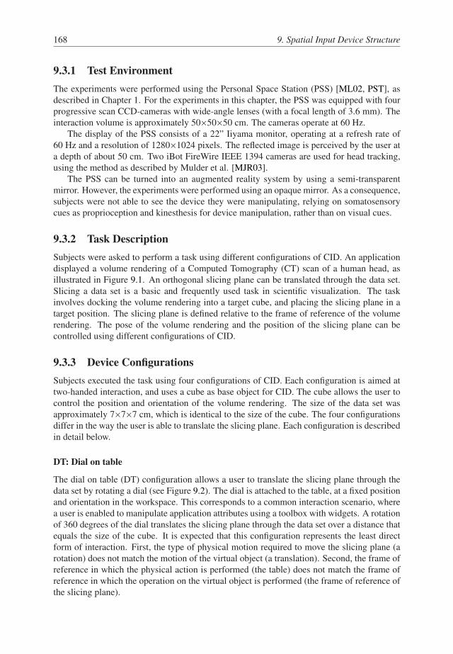
168 9. Spatial Input Device Structure
9.3.1 Test Environment
The experiments were performed using the Personal Space Station (PSS) [ML02, PST], as
described in Chapter 1. For the experiments in this chapter, the PSS was equipped with four
progressive scan CCD-cameras with wide-angle lenses (with a focal length of 3.6 mm). The
interaction volume is approximately 50�50�50 cm. The cameras operate at 60 Hz.
The display of the PSS consists of a 22” Iiyama monitor, operating at a refresh rate of
60 Hz and a resolution of 1280�1024 pixels. The reflected image is perceived by the user at
a depth of about 50 cm. Two iBot FireWire IEEE 1394 cameras are used for head tracking,
using the method as described by Mulder et al. [MJR03].
The PSS can be turned into an augmented reality system by using a semi-transparent
mirror. However, the experiments were performed using an opaque mirror. As a consequence,
subjects were not able to see the device they were manipulating, relying on somatosensory
cues as proprioception and kinesthesis for device manipulation, rather than on visual cues.
9.3.2 Task Description
Subjects were asked to perform a task using different configurations of CID. An application
displayed a volume rendering of a Computed Tomography (CT) scan of a human head, as
illustrated in Figure 9.1. An orthogonal slicing plane can be translated through the data set.
Slicing a data set is a basic and frequently used task in scientific visualization. The task
involves docking the volume rendering into a target cube, and placing the slicing plane in a
target position. The slicing plane is defined relative to the frame of reference of the volume
rendering. The pose of the volume rendering and the position of the slicing plane can be
controlled using different configurations of CID.
9.3.3 Device Configurations
Subjects executed the task using four configurations of CID. Each configuration is aimed at
two-handed interaction, and uses a cube as base object for CID. The cube allows the user to
control the position and orientation of the volume rendering. The size of the data set was
approximately 7�7�7 cm, which is identical to the size of the cube. The four configurations
differ in the way the user is able to translate the slicing plane. Each configuration is described
in detail below.
DT: Dial on table
The dial on table (DT) configuration allows a user to translate the slicing plane through the
data set by rotating a dial (see Figure 9.2). The dial is attached to the table, at a fixed position
and orientation in the workspace. This corresponds to a common interaction scenario, where
a user is enabled to manipulate application attributes using a toolbox with widgets. A rotation
of 360 degrees of the dial translates the slicing plane through the data set over a distance that
equals the size of the cube. It is expected that this configuration represents the least direct
form of interaction. First, the type of physical motion required to move the slicing plane (a
rotation) does not match the motion of the virtual object (a translation). Second, the frame of
reference in which the physical action is performed (the table) does not match the frame of
reference in which the operation on the virtual object is performed (the frame of reference of
the slicing plane).

9.3. Method 169
Figure 9.1: The docking application. A user can control the position and orientation of a
volume rendering of a CT scan. A slicing plane can be translated through the data. The task
is to dock the volume rendering and position the slicing plane onto the target on the left.
Dial on table (DT) Slider on table (ST)
Dial on cube (DC) Slider on cube (SC)
Figure 9.2: Interface configurations. The cube controls the position and orientation of the
volume rendering as shown in Figure 9.1. The configurations differ in two ways: the type of
actuator that is used to translate the slicing plane (dial or slider) and the frame of reference of
the actuator (same frame of reference as the data set or fixed).

170 9. Spatial Input Device Structure
ST: Slider on table
The slider on table (ST) configuration allows a user to translate the slicing plane using a
slider. The slider is position controlled, and its length is approximately the size of the cube.
Position control is generally accepted to result in higher human performance than rate control
[JRMC80]. Analogous to the DT configuration, the slider is placed on the table, at a fixed
location in the workspace. This configuration is expected to represent more direct interaction
than the DT configuration, since the physical motion required to move the slicing plane is a
translation.
DC: Dial on cube
The dial on cube (DC) configuration allows a user to translate the slicing plane using a dial.
The dial is placed on the cube that is used to control the pose of the volume rendering. There-
fore, the coordinate system of the dial matches the frame of reference of the cube. As a result,
the frame of reference in which the physical action is performed matches the frame of refer-
ence in which the operation on the virtual object is performed. The relation between rotation
direction and slicing plane movement was chosen similar as in case of a screwdriver: rotating
clock-wise moves the slicing plane “into” the data set. Using the screwdriver metaphor, it
is expected that the dial has implicit directional cues for virtual object translation along the
rotation axis.
SC: Slider on cube
The slider on cube (SC) configuration allows a user to translate the slicing plane using a
slider. Analogous to the DC configuration, the slider is placed on the cube that is used to
control the pose of the volume rendering. The position of the slider directly corresponds to
the position of the slicing plane. This configuration is expected to result in the most direct
interaction scenario, where both the type and the frame of reference of the physical motion
matches the resulting motion of the virtual objects.
Hypotheses
From the previous sections, the following hypotheses are defined:
� The configuration in which the type and the frame of reference of the physical motion
matches that of the virtual objects is the most S-R compatible. As a result, the slider
on cube configuration is expected to result in the best performance.
� The configuration in which both the type and frame of reference of the physical motion
does not match that of the virtual objects is the least S-R compatible. As such, the dial
on table configuration is expected to result in lowest performance.
� The configuration in which only the motion type of the physical motion matches that of
the virtual object is more S-R compatible than the configuration where only the frame
of reference matches.
9.3.4 Procedure
Subjects performed multiple trials with all four configurations. Each trial involved docking
a data set onto a target cube, and placing a slicing plane at a target position. Before the

9.3. Method 171
-0.05
-0.04
-0.03
-0.02
-0.01
0
0.01
0.02
0.03
5 6 7
positio
n (
m)
time (s)
-0.03
-0.02
-0.01
0
0.01
0.02
0.03
7 8 9 10 11
positio
n (
m)
time (s)
Figure 9.3: Trajectory examples of moving the slicing plane. (a) A user moved the slicing
plane directly to a target location. (b) A user first moved the slicing plane in an unintended
direction, and then corrected the mistake.
experiment, subjects were made aware of the limitations of the tracking system, and were
instructed to use the handles on the actuators to prevent them from grabbing the markers.
Before commencing with the experiment, subjects were verbally instructed and were
given four training trials for each configuration of CID. Next, subjects performed the task
30 times for each configuration, resulting in 120 recorded trials. The total time subjects took
to complete the experiment was approximately an hour.
After completing the trials for all configurations, subjects were asked to fill in a ques-
tionnaire for subjective ratings. After accessing the subjects’ prior experience with virtual
reality and the PSS, they were asked to give each of the four configurations ratings for overall
impression, comfort, and intuitiveness.
9.3.5 Performance Metrics
Each trial, the time was measured that subjects took to manipulate an actuator. This ma-
nipulation time was obtained by filtering and differentiating the tracking data. Each subject
performed 30 trials for each of the four configurations, resulting in 14 � 30 D 420 measure-
ments of slicing plane manipulation time per configuration.
To check the effect of different configurations on the ability of a user to perform the
docking task, the total task completion time was also measured. Different interface structures
may affect the user’s ability to perform the docking task.
A third performance metric is the chance that a user starts movement of the slicing plane
in the opposite direction of the position of the target. This metric is estimated by measuring
the number of trials that users start movement in the opposite direction. It is expected that
in less direct interaction scenarios, users cannot predict the outcome of their actions. For
instance, in the slider on cube configuration, users are expected to make less manipulation
errors than in the case of a dial on table configuration.
Figure 9.3 shows two example trajectories of the slicing plane. On the left, a user moves
the slicing plane directly in the direction of the target position. The trajectory on the right
shows a typical example of a user initially manipulating the actuator such that the slicing
plane erroneously moves in the opposite direction of the target position. After observing
the unintended movement, the user moves the slicing plane in the correct direction. Inter-
face configurations that have a significantly lower chance of these manipulation errors are
expected to perform better and be more intuitive.

172 9. Spatial Input Device Structure
0
0,5
1
1,5
2
2,5
DT ST DC SC
Configuration
Ma
nip
ula
tio
n t
ime
(s)
Figure 9.4: Slicing plane manipulation times with 95% confidence intervals.
Dial Slider
Mean 95% Mean 95%
Table 1.71 0.08 1.37 0.05
Cube 2.04 0.09 1.25 0.04
Table 9.1: Slicing plane manipulation times with 95% confidence intervals.
9.4 Results
Fourteen right-handed subjects participated (1 female and 13 males). All subjects were used
to working with computers. Seven subjects had little to no prior experience working in the
PSS, and six had moderate to much experience. All subjects reported to have good to excel-
lent depth perception during the trials.
9.4.1 Slicing Plane Manipulation Time
Statistical analysis of the slicing plane manipulation time Ts showed that the logarithm of
time could be approximated well by a Gaussian distribution. The t -distribution was used to
determine a 95% confidence interval for the average log Ts , giving the estimated range of
values which is likely to include log Ts [DS98]. The average values and confidence intervals
were mapped back to duration time to allow for easier interpretation of the results. Figure 9.4
summarizes the results. The vertical lines define the ranges of the 95% confidence intervals.
Table 9.1 summarizes the results of the manipulation times. The figure and table suggest that
the dial configurations perform worse than the slider configurations, and that the slider on
cube configuration performs best.
An analysis of variance (ANOVA) was performed on log Ts , and a highly significant ef-
fect was found for device structure on slicing plane manipulation time (F(3,1676) = 129.5,
p < 0:01). The dial on table configuration performs significantly worse than the slider on
table configuration (F(1,838) = 72.2, p < 0:01). Similarly, the dial on cube configuration

9.4. Results 173
0
2
4
6
8
10
12
14
16
DT ST DC SC
Configuration
Ta
sk c
om
ple
tio
n t
ime
(s)
Figure 9.5: Total task completion times with 95% confidence intervals.
performs significantly worse than the slider on cube (F(1,838) = 288.8, p < 0:01) configu-
ration. The slider on table configuration perform significantly worse than the slider on cube
configuration (F(1,838) = 13.2, p < 0:01). Interestingly, the dial on table configuration per-
forms significantly better than the dial on cube configuration (F(1,838) = 35.3, p < 0:01).
These results are discussed in more detail in Section 9.5.
9.4.2 Total Task Completion Time
The total task completion time Tt is analyzed in the same way as the slicing plane manip-
ulation time. A 95% confidence interval for the average log Tt was determined to give the
estimated range of values which is likely to include log Tt . The results, mapped back to
duration time, are summarized in Figure 9.5.
An analysis of variance (ANOVA) was performed on log Tt , and a significant effect was
found for device structure on total task completion time (F(3,1676) = 45.5, p < 0:01). The
dial on table configuration performs significantly worse than the slider on table configuration
(F(1,838) = 10.53, p < 0:01). No significant effect was found between the dial on table
and dial on cube configurations (F(1,838) = 0.88, p > 0:1). The slider on cube configuration
performs significantly better than the dial on cube (F(1,838) = 95.0, p < 0:01), slider on table
(F(1,838) = 50.6, p < 0:01), and dial on table (F(1,838) = 103.7, p < 0:01) configurations.
Comparing these results with the slicing plane manipulation times, there is no significant
statistical evidence to assume users are extra hampered in performing the task in either the
cube configurations or the table configurations.
9.4.3 Manipulation Error Chances
The 95% confidence intervals for samples from the Binomial distribution were calculated for
the chance of manipulation errors [YMS03]. Figure 9.6 summarizes the results. The figure
suggests that the error chance is lowest in the slider on cube configuration. To test if the error
chance of the configurations corresponds to 0.5, a binomial test is performed. If the error
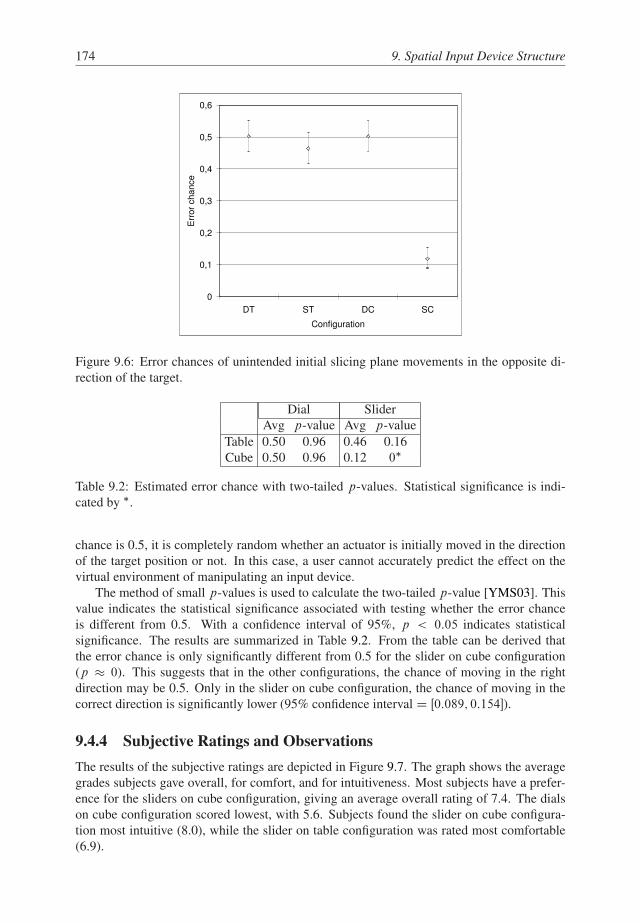
174 9. Spatial Input Device Structure
0
0,1
0,2
0,3
0,4
0,5
0,6
DT ST DC SC
Configuration
Err
or
ch
an
ce
Figure 9.6: Error chances of unintended initial slicing plane movements in the opposite di-
rection of the target.
Dial Slider
Avg p-value Avg p-value
Table 0.50 0.96 0.46 0.16
Cube 0.50 0.96 0.12 0�
Table 9.2: Estimated error chance with two-tailed p-values. Statistical significance is indi-
cated by �.
chance is 0.5, it is completely random whether an actuator is initially moved in the direction
of the target position or not. In this case, a user cannot accurately predict the effect on the
virtual environment of manipulating an input device.
The method of small p-values is used to calculate the two-tailed p-value [YMS03]. This
value indicates the statistical significance associated with testing whether the error chance
is different from 0.5. With a confidence interval of 95%, p < 0:05 indicates statistical
significance. The results are summarized in Table 9.2. From the table can be derived that
the error chance is only significantly different from 0.5 for the slider on cube configuration
(p � 0). This suggests that in the other configurations, the chance of moving in the right
direction may be 0.5. Only in the slider on cube configuration, the chance of moving in the
correct direction is significantly lower (95% confidence interval D Œ0:089; 0:154�).
9.4.4 Subjective Ratings and Observations
The results of the subjective ratings are depicted in Figure 9.7. The graph shows the average
grades subjects gave overall, for comfort, and for intuitiveness. Most subjects have a prefer-
ence for the sliders on cube configuration, giving an average overall rating of 7.4. The dials
on cube configuration scored lowest, with 5.6. Subjects found the slider on cube configura-
tion most intuitive (8.0), while the slider on table configuration was rated most comfortable
(6.9).

9.4. Results 175
0
1
2
3
4
5
6
7
8
9
Overall Comfort Intuitiveness
Ra
tin
g
DT
ST
DC
SC
Figure 9.7: Average subject ratings on overall impression, comfort, and intuitiveness of op-
erating the device structure.
It was found that 9 out of 14 subjects reported to prefer the slider on cube configuration,
followed by 4 for the slider on table configuration and 2 for the dial on table configuration.
When asked further, most subjects that did not rate the sliders on cube configuration the
overall best indicated that the slider on cube configuration was indeed more intuitive, but that
they regarded comfort more important than intuitiveness.
Various subjects reported that manipulating the input device felt more comfortable in the
table configurations. They stated that docking the data set was more difficult in the actuator on
cube configurations, because the cube was more obtrusive to handle with an actuator attached
to it. Furthermore, it was observed that in the actuator on cube configurations, subjects have
difficulties performing the task when the target is oriented such that the actuator has to be
manipulated on the left side of the base object. This resulted in subjects passing CID over
from their non-dominant to their dominant hand, and manipulating the actuator with their
non-dominant hand. Some subjects insisted on manipulating the actuator with their dominant
hand like in other situations, resulting in crossing of hands to manipulate the actuator on the
left side. As a result, subjects lost accuracy and speed while manipulating the actuator. Some
subjects reported slightly more tracking issues, caused by occlusion of the markers by the
hands.
All subjects were found to perform the docking of the data set and the positioning of the
slicing plane serially. This indicates that the pose of the data set and the position of the slicing
plane are perceived as independent attributes.
In the table configurations, some subjects docked the data set with two hands and then
searched for the actuators on the table. Others held the data set in the non-dominant hand and
held the dominant hand on the actuator all the time. The latter group of subjects generally
had more prior VR experience.

176 9. Spatial Input Device Structure
9.5 Discussion
9.5.1 Motion Type
Figure 9.4 shows that manipulation times of the slider configurations are both lower than
the dial configurations. Taking the difference of log T between the slider on table and dial
on table configurations, the logarithm of the ratio between the manipulation times of the
configurations is obtained. Taking the exponential, it is found that on average, the dial on
table configuration is 1.25 times slower than the slider on table configuration. A similar
analysis reveals that the dial on cube configuration is 1.63 times slower than the slider on cube
configuration. This indicates that rotating a dial to move a slicing plane results in a 1.25 to
1.63 times lower S-R compatibility than translating a slider. As such, it may be advantageous
to match the type of a user’s action to the corresponding observed virtual object motion.
The manipulation error chances and the binomial test summarized in Table 9.2 suggest
that subjects do not know which way to rotate the dial to move the slicing plane to a given
location, even if the dial is placed in the correct frame of reference. This indicates that merely
matching the frames of reference of a user’s action and the virtual object is not sufficient. In
this case, visual and somatosensory cues of the user’s action and the perceived effect in the
virtual environment are not in agreement.
Although there is not enough evidence to support the claim that the error chance is 0.5
in the slider on table configuration (with a two-tailed p-value of 0.16), some subjects stated
that they could feel if the slider was up or down, and could use this information to move the
slicing plane in the correct direction during the next trial.
The slider on table configuration is the most intuitive with respect to slicing plane move-
ment, with a two-tailed p < 0:05 and a 95% confidence interval of the error chance of
Œ0:089; 0:154�.
9.5.2 Frame of Reference
The slider on cube configuration has significantly lower manipulation times, with times of
73% of the dial on table configuration, 61% of the dial on cube configuration, and 88%
of the slider on table configuration. This suggests that this configuration is the most S-R
compatible. Therefore, it is desirable to match the frames of reference of a user’s action and
of the corresponding observed virtual object. However, the dial configurations do not show
similar results. On the contrary, the dial on cube configuration performs 1.2 times slower
than the dial on table configuration. This may be explained by Fitt’s law [Fit54, FP64]. Fitt’s
law describes the time taken to acquire a visual target using a manual input device. It can be
described as
T D C1 C C2 CD (9.1)
where D represents the index of difficulty of the task, which depends in the distance to the
center of the target and the target width, and where C1 and C2 are experimentally determined
constants. The quantity 1=C2 is called the index of performance. Previous work suggests that
especially for relatively small distances and small targets, the index of performance is larger
for the dominant hand than for the non-dominant hand [Flo75, KMB93]. In the cube con-
figurations, subjects were sometimes forced to either operate the dial with the non-dominant
hand, or to cross hands to operate the dial (see Section 9.4.4). Therefore, task performance is
decreased in cases where the actuator is on the opposite side of the user’s dominant hand.

9.6. Conclusion 177
Additionally, subjects could not profit from the benefits of having the dial in the same
frame of reference as the observed motion of the slicing plane, as the motion types did not
match. This is supported by Figure 9.6, which indicates that the manipulation error chance
is around 0.5 for both dial configurations. However, the error chance of the slider on cube
configuration is significantly lower. This indicates that the slider on cube configuration en-
ables subjects best to predict the outcome of their manipulations, resulting in more natural
and intuitive interaction.
9.5.3 Intuitiveness versus Comfort
The subjective ratings (see Figure 9.7) show that subjects generally find the slider on cube
configuration most intuitive, followed by the slider on table configuration. However, subjects
rated the slider on table configuration better in terms of comfort. This indicates that there is
a tradeoff between intuitiveness and comfort in designing spatial input devices. The slider
on cube configuration allows for more direct and natural interaction, but is less comfortable
and therefore more tiring than the table variant. However, it may be possible to reduce this
gap in comfort. The most important reason subjects gave for their comfort ratings is the fact
that the actuator on the base object hampers the user somewhat during the docking of the
data set. However, results indicate that this does not have a significant performance impact.
Furthermore, many applications do not require the repeated docking of an object, but simply
use an input device to allow a user to view a data set from different angles. Furthermore,
the ergonomics of CID could be improved and the size of the actuators reduced to increase
comfort.
9.5.4 Design Principles
The design principles for the slicing plane positioning task can be summarized as follows:
� Human performance increases when a device is structured such that both the motion
type and frame of reference of a user’s physical action match the motion type and frame
of reference of the virtual object being manipulated.
� It may be more comfortable and beneficial for task performance if users are able to
manipulate the actuator with their dominant hand.
� For tasks that require much manipulation of the base object of CID, the slider on table
configuration may be a good alternative to increase user comfort, at the expense of
lower human performance.
9.6 Conclusion
In this chapter, the effects were studied of matching the spatial structure of an input device to a
3D interaction task on aspects like effectiveness, intuitiveness, and comfort. A user study was
performed using CID, an optically tracked configurable interaction device. This device allows
for rapid development and evaluation of different device structures. Subjects were asked to
perform a task in which they had to dock a data set to a target position and orientation, and
position a slicing plane through this data set. The slicing plane was positioned along an axis
that was defined in the frame of reference of the data set.

178 9. Spatial Input Device Structure
The device was structured in four different ways, varying the frame of reference and
type of the physical action that needs to be performed. The frame of reference of the device
used for translating the slicing plane through the data set was either identical to the frame
of reference of the data set, or was kept at a fixed, separately located, frame of reference.
The type of action was varied by using either a slider or a dial to translate the slicing plane.
Subjects could control the position and orientation of the data set in each configuration using
a cube-shaped object.
Results show that the structure of a device influences S-R compatibility. It can be advan-
tageous to structure a device such that both motion type and frame of reference of a user’s
action match the frame of reference and type of motion of the virtual object being manip-
ulated. It was found that matching only the frame of reference may degrade performance,
since users do not have enough information to efficiently position the slicing plane using a
dial. This is expected to be true for other motion types as well.
An interesting result is that users generally found the device structures with the widget at
a fixed location more comfortable to manipulate. However, the use of a slider attached to a
cube was generally found to be most intuitive. More research can be done to study this effect
further.
It was also found that users perform the docking of the data set and the positioning of the
slicing plane serially. This indicates that these attributes are perceived as separable. Further
research can be done to test whether these results hold for integral tasks. However, Wang et al.
[WMSB98] found that 3D positioning and orientation only partially exhibit a parallel relation.
More work is needed to determine whether users are capable of perceptually combining more
than six dimensions and manipulating these simultaneously.

Chapter 10
Conclusion
Three-dimensional interaction between a user and a virtual environment is a powerful concept
to manipulate, study, and communicate spatial information. Two aspects play a crucial role
in determining the effectiveness of this interaction process. The first is the display system,
which is used to convey information from the virtual environment to the user. The second
is the input system, which steers the computational processes that control the display. The
research presented in this thesis focussed on the input side of 3D interaction. The research
objective was formulated as:
The development and application of configurable input devices for direct 3D
interaction in near-field virtual environments using optical tracking.
The concepts and techniques presented in this thesis have been implemented and evaluated
in the Personal Space Station, the virtual environment developed at CWI.
In the next section, the contributions of this thesis and the developed concepts and tech-
niques are summarized. In Section 10.2, suggestions for valuable extensions and future work
are given.
10.1 Contributions
Optical Motion Tracking
A number of lessons were learned during the development and evaluation of the optical track-
ing techniques used for the configurable interaction device:
� The selection of the best tracking technique depends on the requirements as defined
in Chapter 1, and on which of these requirements are considered most important for a
given virtual environment.
The tracking technique based on finding subgraph isomorphisms of point features in
three-dimensional space is accurate and has low latency. Furthermore, it is better suited
to handle partial occlusion than related pattern-based approaches, since any combina-
tion of a predetermined minimum amount of points is sufficient to recognize the device.
It allows objects of arbitrary shape to be tracked and enables a developer to rapidly con-
struct new devices.
The tracking system that uses projection invariant properties of line pencils is also
accurate and has low latency, and is more robust against partial occlusion and small
camera calibration errors. However, the construction of new interaction devices is more
difficult than the subgraph tracker that uses point features, and the shape of interaction
devices is limited since line pencils are required to be applied to planar surfaces.
179

180 10. Conclusion
� Filtering and prediction strategies provide an effective means for reducing tracker inac-
curacies caused by noise and latency. However, more complex does not always equal
better. For the motion models used in this thesis, a linear time-invariant filter extended
with a simple prediction step based on the motion model was shown to be competitive
to more complex filtering strategies, in case the sampling frequency is sufficiently high
(i.e. larger than 30 Hz).
� The automatic model estimation technique for rigid interaction devices, which is based
on using frame-to-frame correspondence to maintain a graph of points that correspond
to the same rigid object, is a powerful tool for the construction of new interaction
devices. It enables a developer to equip an object with markers, move it around in front
of the cameras, and use the object as interaction device in the virtual environment. The
method supports partial occlusion of the marker sets.
� Composite interaction devices consist of several segments connected in a tree structure.
Segments can have combinations of translational and rotational degrees of freedom
with respect to a parent segment. Such devices can efficiently be tracked by searching
a root segment with the subgraph tracking method, and using a backtracking method
to match model segments to single markers.
The model estimation procedure based on estimating the DOF relation between a mov-
ing marker and a coordinate system provides a convenient way to construct composite
objects and apply them as interaction devices in the virtual environment. It would be
a tedious and error-prone job to construct a composite object and manually measure a
model that describes the DOFs and DOF ranges of each segment.
Configurable Interaction Devices
The optical tracking techniques for composite devices have been used to construct an op-
tically tracked configurable interaction device (CID). CID was shown to enable a user to
manipulate a large number of application parameters with a single, compact device. A devel-
oper can rapidly construct new configurations to experiment with new interaction techniques
and devices. The structure of a configuration of CID can directly reflect the application pa-
rameters, resulting in an intuitive interface.
In Chapter 8, the flexibility of CID was demonstrated in a number of application scenar-
ios, using different interface configurations. The applications range from modeling, scientific
data exploration, and interactive animation. CID allows for the creation of a large number of
new device configurations, specifically tuned to a given application. Furthermore, the devel-
oped tracking techniques allow for automatic model estimation of new device configurations
and for robust estimation of all degrees of freedom of CID.
Spatial Device Structure
CID proved to be a valuable tool for studying the effects of different interface structures on
factors as task performance, intuitiveness, and comfort. It was found that the structure of
a device for a 3D spatial object manipulation task influences stimulus-response compatibil-
ity. This may indicate that the structure of an interaction device should reflect the spatial
parameters of the interaction task at hand. In this case, stimulus-response compatibility is
maximized, which should result in a more direct and intuitive interface.

10.2. Future Work 181
10.2 Future Work
Optical Tracking
The tracking techniques presented in this thesis take a next step towards the ideal tracking
method, i.e., the method that satisfies all requirements listed in Chapter 1. The tracking
technique based on finding subgraph isomorphisms of point features in 3D allows for objects
of arbitrary shape to be tracked, and allows for rapid development of new devices. On the
other hand, the tracking method that uses projection invariant properties of line pencils is
more robust against partial occlusion, while the development of new devices is more difficult
and the shape of devices is restricted. Future work should focus on the development of new
tracking methods that combine the best qualities of these methods.
More extensive models can be developed, using more mathematical rigor. These models
can be used for analytical evaluations of new tracking methods. This results in more accurate
evaluations of tracking methods, providing a means of proving why one method performs bet-
ter than another in a given virtual environment, tracking setup, and application. Additionally,
such models could possibly be used to predict the usefulness of a given tracking approach,
before the approach is realized in practice.
The model estimation procedure for rigid interaction devices as presented in this thesis
could be extended to support faster and more erratic motions during model estimation. This
could be achieved by falling back on the subgraph tracking method in case of loss of frame-
to-frame correspondence. When a part of the (incomplete) device model has been identified
by the tracking method, the normal model estimation procedure can be resumed. A useful and
challenging extension to the model estimation procedure for composite interaction devices is
to support partial occlusion of the marker sets.
Filtering and prediction techniques could benefit from more accurate models to describe
hand motion characteristics in a virtual environment. Such models can be used to create
synthetic signals that act as a performance benchmark for filter and prediction performance
evaluation, as well as to develop more accurate filtering and prediction strategies. Other inter-
esting areas for future work are adaptive and multi-modal filtering, including the development
of a motion model that exploits high level interaction information. For example, the motion
model can be adapted to the task a user performs, exploiting knowledge about the expected
motion speed, direction, and orientation changes.
In this thesis, tracking techniques were developed for determining the 3D position and
orientation of interaction devices. Next, the techniques were extended to support compos-
ite interaction devices, allowing for more degrees of freedom in a single device. The next
step would be to develop tracking methods for deformable objects. Deformable interaction
devices would open up new perspectives for complex 3D interaction tasks. For instance, de-
formable interaction devices could enable a user to model a virtual object by simple pushing
and pulling operations on the surface of the device, enabling a user to “mould” a virtual ob-
ject into a desired shape. An interesting option for the development of a tracking system for
deformable objects would be to exploit the projection invariant property of graph topology
[SRL06].
Configurable Interaction Devices
The research in this thesis has resulted in a framework for the development and application
of new interaction devices for high dimensional input. The next step would be to extend the
182 10. Conclusion
framework to allow for:
� Efficient design and development of interaction devices. This includes the development
of tools to aid the developer in the design and construction of the interaction devices, as
well as to apply the device in the virtual environment using the optical tracking system.
� Effective development of interaction techniques. This involves the mapping of the
degrees of freedom of the device to the parameters of the interaction task, as well
as the development of the visual (or possibly multi-modal) feedback associated with
manipulations of the interaction device.
� Evaluation of interaction devices and techniques. This involves the development of
tools to aid the developer to rapidly set up user experiments and evaluate new interac-
tion devices and techniques, subject to a set of predefined parameters.
CID allows for efficient design and development of interaction devices. The map editor
presented in Chapter 8, which allows a developer to adjust the mapping of the degrees of
freedom of the device and the parameters of the interaction task in real-time, takes the first
step to a framework that allows for efficient development of interaction techniques. The
further development of this framework, including an intuitive user interface to develop and
test new configurations of CID, would allow for the development of new interaction devices
by people who are not computer scientists or tracking experts.
It would be interesting to study if CID can be applied successfully to other application
areas and other virtual environments. Possible application areas include entertainment, mod-
eling, construction, training, simulation, and scientific visualization areas such as geology,
biology, and medicine. The applications of CID and the underlying optical tracking tech-
niques developed in this thesis have been applied and evaluated in the Personal Space Station.
However, the concepts and techniques presented in this thesis could also be applied to other
types of virtual environments, such as workbenches and CAVE systems. Spatially immersive
environments as the CAVE often only provide remote interaction by using simple pointing
devices. CID could enable more direct spatial interaction in such environments, opening up
new interaction perspectives.
Spatial Device Structure
CID can be used to perform more studies to test the driving vision of this thesis under more
circumstances. Although the user study in Chapter 9 indicates that spatial and directional
S-R compatibility plays an important role in human performance, this may not be true in all
cases. For instance, human beings are capable of learning new skills and efficiently operate
interfaces that are seemingly counter-intuitive. However, experimental evidence suggests
that the effects of S-R compatibility can never be fully “trained away” [VP03]. As a result,
even the most experienced users still benefit from compatible mappings between stimuli and
responses. More work is needed to evaluate how much more effective an S-R compatible
interface is compared to an interface with a less compatible mapping, especially if significant
training is allowed.
Another interesting area for further research is to evaluate how many degrees of freedom
should be included in an interaction device for a given interaction task. Some 2D interfaces
use large control panels that allow for the adjustment of many parameters. Similarly, graph-
ical interfaces often have a large number of options and settings that can be selected. Even

10.2. Future Work 183
though the latter example may be operated with a single desktop mouse, these examples show
that interfaces with many degrees of freedom not necessarily become too complex for use.
It seems that human beings are very capable of focussing their attention to a specific part of
an interface. However, evidence suggests that the number of parameters that can be manip-
ulated simultaneously is more limited. For instance, Wang et al. [WMSB98] found that 3D
positioning and orientation are only partially performed in parallel. It would be interesting
to determine how many input dimensions users are capable of perceptually combining and
manipulating in parallel.
An interesting result of the study in Chapter 9 is that the most intuitive interface not neces-
sarily results in the most comfortable interface. For the experiments performed in Chapter 9,
some users preferred a toolbox type of interface over the more intuitive interface, as the hands
could rest more on the table. This leads to the question: “Can an interface be designed such
that both intuitiveness and comfort are maximized?”. The answer to this question, along with
the development of a framework that developers could use to construct interfaces that are both
intuitive and comfortable, would be a significant contribution to the field of virtual reality. It
would enable developers to create truly natural interfaces that can be operated with minimum
effort and for prolonged periods of time.

184 10. Conclusion

References
[AB94] R. Azuma and G. Bishop. Improving static and dynamic registration in a see-
through HMD. In Proceedings of SIGGRAPH’94, pages 197–204. 1994.
[AF98] M. J. Atallah and S. Fox, editors. Algorithms and Theory of Computation Hand-
book. CRC Press, Inc., Boca Raton, FL, USA, 1998. ISBN 0849326494. Pro-
duced By-Suzanne Lassandro.
[AM95] K. Astrom and L. Morin. Random cross ratios. In Proc. 9th Scand. Conf. on
Image Anal., pages 1053–1061. 1995.
[AMGC02] S. Arulampalam, S. Maskell, N. Gordon, and T. Clapp. A tutorial on particle
filters for on-line non-linear/non-gaussian bayesian tracking. IEEE Transactions
on Signal Processing, 50(2):174–188, February 2002.
[AZ96] M. Ayers and R. C. Zeleznik. The lego interface toolkit. In ACM Symposium on
User Interface Software and Technology, pages 97–98. 1996.
[Azu95] R. Azuma. Predictive Tracking for Augmented Reality. Ph.D. thesis, University
of North Carolina at Chapel Hill, 1995.
[BC93] B. Bell and F. Cathey. The iterated kalman filter update as a gauss-newton
method. IEEE Transactions on Automatic Control, 38(2):294–297, 1993.
[BFKS99] R. Balakrishnan, G. Fitzmaurice, G. Kurtenbach, and K. Singh. Exploring in-
teractive curve and surface manipulation using a bend and twist sensitive input
strip. In SI3D ’99: Proceedings of the 1999 symposium on Interactive 3D graph-
ics, pages 111–118. ACM Press, New York, NY, USA, 1999.
[BG62] D. E. Broadbent and M. Gregory. Donders’ b- and c- reactions and S-R com-
patibility. Journal of Experimental Psychology 63, pages 575–578, 1962.
[BH99a] R. Balakrishnan and K. Hinckley. The role of kinesthetic reference frames in
two-handed input performance. In Proceedings of the 12th annual ACM sym-
posium on User interface software and technology, pages 171–178. 1999.
[BH99b] D. Bowman and L. Hodges. Formalizing the design, evaluation, and application
of interaction techniques for immersive virtual environments. The Journal of
Visual Languages and Computing, 10(1):37–53, February 1999.
[BJH01] D. A. Bowman, D. B. Johnson, and L. F. Hodges. Testbed evaluation of vir-
tual environment interaction techniques. Presence: Teleoperators and Virtual
Environments, 10(1):75–95, February 2001.
185

186 References
[BKLP01] D. A. Bowman, E. Kruijff, J. J. LaViola Jr, and I. Poupyrev. An introduction
to 3D user interface design. Presence: Teleoperators and Virtual Environments,
10(1):96–108, February 2001.
[BM92] P. J. Besl and N. D. McKay. A method for registration of 3-D shapes. IEEE
Transactions on Pattern Analysis and Machine Intelligence, 14(2):239–256,
1992.
[Bro99] F. P. Brooks Jr. What’s real about virtual reality? IEEE Computer Graphics and
Applications, 19(6):16–27, 1999.
[BSF88] Y. Bar-Shalom and T. E. Fortmann. Tracking and Data Association. Academic
Press, 1988.
[BT80] S. Barnard and W. Thompson. Disparity analysis of images. IEEE Trans. Pat-
tern Anal. Machine Intell, pages 333–340, 1980.
[BT98] S. Birchfield and C. Tomasi. Depth discontinuities by pixel-to-pixel stereo. In
Proceedings of the Sixth IEEE International Conference on Computer Vision,
pages 1073–1080. 1998.
[CFSV04] L. P. Cordella, P. Foggia, C. Sansone, and M. Vento. A (sub)graph isomorphism
algorithm for matching large graphs. IEEE Trans. Pattern Anal. Mach. Intell.,
26(10):1367–1372, 2004.
[CH99] S. Christy and R. Horaud. Iterative pose computation from line correspon-
dences. Computer Vision and Image Understanding, 73(1):137–144, January
1999.
[Che91] H. Chen. Pose determination from line-to-plane correspondences: existence
condition and closed-form solutions. IEEE Transactions on pattern analysis
and machine intelligence, 13(6):530–541, June 1991.
[Chv83] Q. V. Chvatal. Linear Programming. W. H. Freeman and Co., 1983.
[CMR90] S. Card, J. Mackinlay, and G. Robertson. The design space of input devices. In
Proceedings of CHI, pages 117–124. 1990.
[CNHV99] L. Chai, K. Nguyen, B. Hoff, and T. Vincent. An adaptive estimator for reg-
istration in augmented reality. In Proc. of 2nd IEEE/ACM Int’l Workshop on
Augmented Reality (IWAR ’99). October 1999.
[CNX] 3DConnexion, http://www.3dconnexion.com/.
[CS00] J-X. Chai and H-Y. Shum. Parallel projections for stereo reconstruction. In Pro-
ceedings of the IEEE Conference on Computer Vision and Pattern Recognition,
volume 2, pages 493–500. 2000.
[CTCG95] T. Cootes, C. Taylor, D. Cooper, and J. Graham. Active shape models - their
training and application. Computer Vision and Image Understanding, 61(1):38–
59, 1995.

References 187
[CW99] S. Coquillart and G. Wesche. The virtual palette and the virtual remote con-
trol panel: A device and an interaction paradigm for the responsive work-
bench((tm)). In VR ’99: Proceedings of the IEEE Virtual Reality Conference,
pages 13–17. IEEE Computer Society, Washington, DC, USA, 1999.
[DGK01] A. Doucet, N. J. Gordon, and V. Krishnamurthy. Particle filters for state estima-
tion of jump markov linear systems. IEEE Transactions on Signal Processing,
49(3):613–624, 2001.
[DH72] R. O. Duda and P. E. Hart. Use of the hough transformation to detect lines and
curves in pictures. Communications of the ACM, 15(1):11–15, 1972.
[Dor99] K. Dorfmuller. Robust tracking for augmented reality using retroreflective
markers. Computers and Graphics, 23(6):795–800, 1999.
[Dou98] A. Doucet. On sequential monte carlo methods for bayesian filtering. Technical
report, University of Cambride, UK, Department of Engineering, 1998.
[DS98] N. R. Draper and H. Smith. Applied Regression Analysis. John Wiley & Sons,
third edition, 1998.
[ET98] S. Emura and S. Tachi. Multisensor integrated prediction for virtual real-
ity. Presence: Teleoperators and Virtual Environments, 7(4):410–422, August
1998.
[EYAE99] S. R. Ellis, M. J. Young, B. D. Adelstein, and S. M. Ehrlich. Discrimination
of changes of latency during voluntary hand movement of virtual objects. In
Proceedings of the Human Factors and Ergonomics Society. 1999.
[FB81] M. A. Fischler and R. C. Bolles. Random sample consensus: a paradigm for
model fitting with applications to image analysis and automated cartography.
Commun. ACM, 24(6):381–395, 1981.
[Fia05] M. Fiala. ARTag, a fiducial marker system using digital techniques. In CVPR
’05: Proceedings of the 2005 IEEE Computer Society Conference on Computer
Vision and Pattern Recognition (CVPR’05) - Volume 2, pages 590–596. IEEE
Computer Society, Washington, DC, USA, 2005.
[FIB95] G. W. Fitzmaurice, H. Ishii, and W. Buxton. Bricks: laying the foundations for
graspable user interfaces. In CHI ’95: Proceedings of the SIGCHI conference
on Human factors in computing systems, pages 442–449. ACM Press/Addison-
Wesley Publishing Co., New York, NY, USA, 1995.
[Fit54] P. M. Fitts. The information capacity of the human motor system in controlling
the amplitude of movement. Journal of Experimental Psychology, 47:381–391,
1954.
[Flo75] K. Flowers. Handedness and controlled movement. British Journal of Psychol-
ogy, 66:39–52, 1975.
[FP64] P. M. Fitts and J. R. Peterson. Information capacity of discrete motor responses.
Journal of Experimental Psychology, 67:103–112, 1964.

188 References
[FP00] B. Frohlich and J. Plate. The cubic mouse: A new device for 3D input. In Proc.
ACM CHI 2000, pages 526–531. ACM Press, New York, 2000.
[FP02] D. A. Forsyth and J. Ponce. Computer Vision: A Modern Approach. Prentice
Hall, 2002. ISBN 0130851981.
[FS53] P. M. Fitts and C. M. Seeger. S-R compatibility: Spatial characteristics of stim-
ulus and response codes. Journal of Experimental Psychology, 46:199–210,
1953.
[Gar74] W. Garner. The Processing of Information and Structure. Wiley, New York,
1974.
[GSS93] N. J. Gordon, D. J. Salmond, and A. F. M. Smith. Novel approach to
nonlinear/non-gaussian bayesian state estimation. In IEEE Proceedings on
Radar and Signal Processing, volume 140, pages 107–113. 1993.
[Gui87] Y. Guiard. Assymetric division of labor in skilled bimanual action: The kine-
matic chain as a model. Journal of Motor Behavior, 19:486–517, 1987.
[HHN86] E. L. Hutchins, J. D. Hollan, and D. A. Norman. Direct manipulation interfaces.
In D. A. Norman and S. W. Draper, editors, User Centered System Design:
New Perspectives on Human-Computer Interaction, pages 87–124. Erlbaum,
Hillsdale, NJ, 1986.
[Hor87] B. K. P. Horn. Closed-form solution of absolute orientation using unit quater-
nions. Journal of the Optical Society of America, A, 4(4):629–642, 1987.
[HPGK94] K. Hinckley, R. Pausch, J. C. Goble, and N. F. Kassell. Passive real-world
interface props for neurosurgical visualization. In CHI ’94: Proceedings of the
SIGCHI conference on Human factors in computing systems, pages 452–458.
ACM Press, New York, NY, USA, 1994.
[HS97] J. Heikkila and O. Silven. A four-step camera calibration procedure with im-
plicit image correction. Computer Vision and Pattern Recognition, pages 1106–
1113, 1997.
[HSDK05] A. Hornung, S. Sar-Dessai, and L. Kobbelt. Self-calibrating optical motion
tracking for articulated bodies. In Proceedings of the IEEE Virtual Reality Con-
ference, pages 75–82. 2005.
[HUHF03] L. Herda, R. Urtasun, A. Hanson, and P. Fua. Automatic determination of joint
limits using quaternion field boundaries. International Journal for Robotis Re-
search, 22(6):419–436, 2003.
[HV00] W. Hoff and T. Vincent. Analysis of head pose accuracy in augmented real-
ity. IEEE Transactions on Visualization and Computer Graphics, 6(4):319–334,
2000. ISSN 1077-2626. doi:http://dx.doi.org/10.1109/2945.895877.
[IB98] M. Isard and A. Blake. Condensation - conditional density propagation for
visual tracking. Int. J. Computer Vision, 29:5–28, 1998.
References 189
[JHWB78] R. J. Jagacinski, E. J. Hartzell, S. Ward, and K. Bishop. Fitts’ law as a function
of system dynamics and target uncertainty. Journal of Motor Behavior, 10:123–
131, 1978.
[Jol02] I. T. Jolliffe. Principal Component Analysis. Springer; 2nd edition, 2002.
[JRMC80] R. J. Jagacinski, D. W. Repperger, M. S. Moran, S. L. Ward, and B. Class. Fitts’
law and the microstructure of rapid discrete movements. Journal of Experimen-
tal Psychology: Human Perception and Performance, 6(2):309–320, 1980.
[JS92] R. J. K. Jacob and L. E. Sibert. The perceptual structure of multidimensional
input device selection. In CHI ’92: Proceedings of the SIGCHI conference on
Human factors in computing systems, pages 211–218. ACM Press, New York,
NY, USA, 1992.
[JSMC94] R. J. K. Jacob, L. E. Sibert, D. C. McFarlane, M. Preston, and J. R. Mullen.
Integrality and separability of input devices. ACM Transactions on Computer-
Human Interaction, 1(1):3–26, 1994.
[JU97] S. J. Julier and J. K. Uhlmann. A new extension of the kalman filter to nonlinear
systems. Int. Symp. Aerospace/Defense Sensing, Simulation and Controls, 1997.
[KB99] H. Kato and M. Billinghurst. Marker tracking and HMD calibration for a video-
based augmented reality conferencing system. In IWAR ’99: Proceedings of
the 2nd IEEE and ACM International Workshop on Augmented Reality, pages
85–94. IEEE Computer Society, Washington, DC, USA, 1999.
[KBS94] P. Kabbash, W. Buxton, and A. Sellen. Two-handed input in a compound task.
In CHI ’94: Conference companion on Human factors in computing systems.
1994.
[KHYN02] K. Kurihara, S. Hoshino, K. Yamane, and Y. Nakamura. Optical motion capture
system with pan-tilt camera tracking and realtime data processing. In Proc. of
IEEE International Conference on Robotics and Automation(ICRA2002), vol-
ume 2, pages 1241–1248. May 2002.
[KL04] A. J. F. Kok and R. van Liere. Co-location and tactile feedback for 2d widget
manipulation. In Proceedings of the IEEE Virtual Reality Conference 2004.
March 2004.
[KMB93] P. Kabbash, I. S. MacKenzie, and W. Buxton. Human performance using com-
puter input devices in the preferred and non-preferred hands. In Proceedings of
InterCHI ’93, pages 474–481. 1993.
[KTES87] W. S. Kim, F. Tendick, S. R. Ellis, and L. W. Stark. A comparison of position
and rate control for telemanipulation with consideration of manipulator system
dynamics. IEEE Journal of Robotics and Automation, 3:426–436, 1987.
[Lau01] M. Laurent. Matrix completion problems. Matrix completion problems. The
Encyclopedia of Optimization, 3:221–229, 2001.

190 References
[LaV03] J. J. LaViola Jr. A comparison of unscented and extended kalman filtering for
estimating quaternion motion. In Proc. 2003 Am. Control Conf., pages 2435–
2440. June 2003.
[LF05] V. Lepetit and P. Fua. Monocular model-based 3D tracking of rigid objects: A
survey. Foundations and Trends in Computer Graphics and Vision, 1(1):1–89,
2005.
[LM03] R. van Liere and J. D. Mulder. Optical tracking using projective invariant marker
pattern properties. Proceedings of the IEEE Virtual Reality 2003 Conference,
pages 191–198, 2003.
[LPNC06] C. Liu, W. Pei, S. Niyokindi, J. C. Song, and L. D. Wang. Micro stereo
matching based on wavelet transform and projective invariance. Seventh Inter-
national Symposium on Measurement Technology and Intelligent Instruments,
17(3):565–571, 2006.
[LR03] R. van Liere and A. van Rhijn. Search space reduction in optical tracking. In
Proceedings of the workshop on Virtual environments 2003, pages 207–214.
ACM Press, 2003.
[LR04] R. van Liere and A. van Rhijn. An experimental comparison of three optical
trackers for model based pose determination in virtual reality. In Proceedings of
the Eurographics Symposium on Virtual Environments, pages 25–34. June 2004.
[LS00a] J. Lasenby and A. Stevenson. Using geometric algebra for optical motion cap-
ture. Geometric algebra: a geometric approach to computer vision, neural and
quantum computing, robotics and engineering, pages 147–169, 2000.
[LS00b] J. Lee and S. Y. Shin. General construction of time-domain filters for orientation
data. IEEE Transaction on Visualization and Computer Graphics, 8:119–128,
2000.
[LSW88] Y. Lamdan, J. T. Schwartz, and H. J. Wolfson. On recognition of 3-D objects
from 2-D images. In Proceedings of IEEE Int. Conf. on Robotics and Automa-
tion, pages 1407–1413. 1988.
[May79] P. S. Maybeck. Stochastic Models, Estimation and Control, Volume 1. Academic
Press, 1979.
[May95] S. J. Maybank. Probabilistic analysis of the application of the cross ratio to
model based vision: Misclassification. Intl. J. of Computer Vision, 14:199–210,
1995.
[MBS97] M. R. Mine, F. P. Brooks Jr, and C. H. Sequin. Moving objects in space: Ex-
ploiting proprioception in virtual-environment interaction. In SIGGRAPH 97
Conference Proceedings, pages 19–26. 1997.
[MDFW00] R. Merwe, A. Doucet, N. Freitas, and E. Wan. The unscented particle filter.
Technical Report CUED/F-INFENG/TR380, Cambridge University, Engineer-
ing Department, August 2000, 2000.

References 191
[Mei71] D. Meister. Human Factors: Theory and Practice. Wiley-Interscience, 1971.
[MFDW01] R. van der Merwe, N. de Freitas, A. Doucet, and E. Wan. The unscented particle
filter. In Advances in Neural Information Processing Systems 13. November
2001.
[Min93] M. R. Mine. Characterization of end-to-end delays in head-mounted display
systems. Technical Report TR93-001, UNC Chapel Hill, Computer Science,
1993.
[MJR03] J. D. Mulder, J. Jansen, and A. van Rhijn. An affordable optical head track-
ing system for desktop VR/AR systems. In J. Deisinger and A. Kunz, editors,
Proceedings of the Workshop on Virtual Environments 2003, pages 215–223.
2003.
[MKM90] D. Mendlovic, N. Konforti, and E. Marom. Shift and projection invariant pattern
recognition using logarithmic harmonics. Appl. Opt., 29:4784–4789, 1990.
[ML02] J. D. Mulder and R. van Liere. The personal space station: Bringing interaction
within reach. In S. Richer, P. Richard, and B. Taravel, editors, Proceedings of
the Virtual Reality International Conference, VRIC 2002, pages 73–81. 2002.
[MLR98] P. Meer, R. Lenz, and S. Ramakrishna. Efficient invariant representations. IJCV,
26(2):137–152, 1998.
[MN00] S. Mills and K. Novins. Motion segmentation in long image sequences. In Pro-
ceedings of the British Machine Vision Conference (BMVC2000), pages 162–
171. 2000.
[MRWB03] M. Meehan, S. Razzaque, M. Whitton, and F. P. Brooks Jr. Effect of latency on
presence in stressful virtual environments. In Proceedings of the IEEE Virtual
Reality Conference, pages 141–148. 2003.
[NM65] J. A. Nelder and R. Mead. A simplex method for function minimization. Com-
put. J., 7:308–313, 1965.
[OBBH00] J. F. O’Brien, R. E. Bodenheimer, G. J. Brostow, and J. K. Hodgins. Auto-
matic joint parameter estimation from magnetic motion capture data. In Proc.
Graphics Interface, pages 53–60. 2000.
[O’R85] J. O’Rourke. Finding minimal enclosing boxes. International Journal of Com-
puter and Information Sciences, 14(3):183–199, 1985.
[Pil97] M. Pilu. A direct method for stereo correspondence based on singular value
decomposition. In Proc. IEEE International Conference of Computer Vision
and Pattern Recognition, pages 261–266. 1997.
[PMF85] S. B. Pollard, J. E. Mayhew, and G. P. Frisby. PMF: A stereo correspondence
algorithm using a disparity gradient limit. Perception, 14:449–470, 1985.
[PS99] M. K. Pitt and N. Shepard. Filtering via simulation: Auxiliary particle filters.
Journal of the American Statistical Association, 94(446):590–599, 1999.

192 References
[PST] Personal Space Technologies, http://www.personalspacetechnologies.com/.
[QL99] L. Quan and Z. Lan. Linear N-point camera pose determination. IEEE Trans.
Pattern Anal. Mach. Intell., 21(8):774–780, 1999.
[RDB00] J. P. Rolland, L. D. Davis, and Y. Baillot. A survey of tracking technology for
virtual environments. In Barfield and Caudell, editors, Fundamentals of Wear-
able Computers and Augmented Reality, pages 67–112. Mahwah, NJ, 2000.
[Rey03] O. Reynhout. Improving optical tracking for the Personal Space Station. Mas-
ter’s thesis, Technische Universiteit Eindhoven, 2003.
[RL02] M. Ringer and J. Lasenby. A procedure for automatically estimating model
parameters in optical motion capture. In British Machine Vision Conference,
pages 747–756. 2002.
[RLM05] A. van Rhijn, R. van Liere, and J. D. Mulder. An analysis of orientation pre-
diction and filtering methods for VR/AR. In Proceedings of the IEEE Virtual
Reality Conference 2005, pages 67–74. March 2005.
[RM04] A. van Rhijn and J. D. Mulder. Optical tracking using line pencil fiducials.
In Proceedings of the Eurographics Symposium on Virtual Environments 2004,
pages 35–44. 2004.
[RM05] A. van Rhijn and J. D. Mulder. Optical tracking and calibration of tangible
interaction devices. In Proceedings of the Immersive Projection Technology
and Virtual Environments Workshop 2005, pages 41–50. 2005.
[RM06a] A. van Rhijn and J. D. Mulder. CID: An optically tracked configurable interac-
tion device. In Proceedings of Laval Virtual International Conference on Virtual
Reality 2006. 2006.
[RM06b] A. van Rhijn and J. D. Mulder. Optical tracking and automatic model estimation
of composite interaction devices. In Proceedings of the IEEE Virtual Reality
Conference 2006, pages 135–142. Alexandria, Virginia, USA, 2006.
[RM06c] A. van Rhijn and J. D. Mulder. Spatial input device structure and bimanual
object manipulation in virtual environments. In Accepted for publication at the
ACM Symposium on Virtual Reality Software and Technology. 2006.
[RPF01] M. Ribo, A. Pinz, and A. Fuhrmann. A new optical tracking system for virtual
and augmented reality applications. In Proceedings of the IEEE Instrumen-
tation and Measurement Technical Conference, volume 3, pages 1932–1936.
Budapest, Hungary, 2001.
[SAM03] S. Subramanian, D. Aliakseyeu, and J-B. Martens. Empirical evaluation of per-
formance in hybrid 3d and 2d interfaces. In Proceedings of Interact 2003, pages
916–919. September 2003.
[SCTM95] P. Sozou, T. Cootes, C. Taylor, and E. Di Mauro. Non-linear point distribution
modelling using a multi-layer perceptron. British Machine Vision Conference
(BMVC’95), pages 107–116, 1995.

References 193
[SF03] A. Simon and B. Frohlich. The YoYo: A handheld device combining elastic and
isotonic input. In Proc. of INTERACT 2003, pages 303–310. 2003.
[Sha98] C. M. Shakarji. Least-squares fitting algorithms of the NIST algorithm testing
system. Journal of Research of the National Institute of Standards and Technol-
ogy, 103(6):633–641, 1998.
[Sho85] K. Shoemake. Animating rotation with quaternion curves. Computer Graphics,
19:245–254, 1985.
[SLH91] G. Scott and H. Longuet-Higgins. An algorithm for associating the features of
two patterns. In Proc. Royal Society London, volume B244, pages 21–26. 1991.
[Smi95] S. M. Smith. ASSET-2: Real-time motion segmentation and shape tracking. In
Proc. 5th Int. Conf. on Computer Vision, pages 237–244. 1995.
[SPBC98] M. Silaghi, R. Plaenkers, R. Boulic, P. Fua, and D. Thalmann. Local and global
skeleton fitting techniques for optical motion capture. Lecture Notes in Com-
puter Science, 1537:26–40, 1998.
[SRL06] F. A. Smit, A. van Rhijn, and R. van Liere. A topology projection invariant
optical tracker. In Proceedings of the Eurographics Symposium on Virtual En-
vironments 2006, pages 63–70. Lisbon, Portugal, May 2006.
[SS02] D. Scharstein and R. Szeliski. A taxonomy and evaluation of dense two-frame
stereo correspondence algorithms. Int. J. Comput. Vision, 47(1-3):7–42, 2002.
[Sug94] A. Sugimoto. Geometric invariant of noncoplanar lines in a single view. Proc.
12th IAPR Int. Conf. on Pattern Recognition (ICPR’94), 10:190–195, 1994.
[Sut65] I. Sutherland. The ultimate display. In Information Processing 1965: Proceed-
ings of IFIP Congress 65, pages 506–508. 1965.
[SW01] T. Schank and D. Wagner. Finding, counting and listing all triangles in large
graphs, an experimental study. Technical Report TR-043, DELIS, 2001.
[Tla04] M. Tlauka. Display-control compatibility: The relationship between perfor-
mance and judgments of performance. Ergonomics, 47(3):281–295, 2004.
[Tou83] G. T. Toussaint. Solving geometric problems with the rotating calipers. In Proc.
IEEE MELECON’83. Athens, Greece, 1983.
[Tsa86] R. Y. Tsai. An efficient and accurate camera calibration technique for 3D ma-
chine vision. In Proceedings of IEEE Conference on Computer Vision and Pat-
tern Recognition, pages 364–374. 1986.
[Van94] D. VanArsdale. Homogeneous transformation matrices for computer graphics.
Computers and Graphics, 18(2):177–191, 1994.
[VIC] Vicon, http://www.vicon.com/.
[VP03] K. L. Vu and R. W. Proctor. Naıve and experienced judgments of stimulus-
response compatibility: Implications for interface design. Ergonomics,
46(1):169–187, 2003.

194 References
[VY86] A. Verri and A. Yuille. Perspective projection invariants. Technical Report
AIM-832, Massachusetts Institute of Technology, 1986.
[WA04] C. Ware and R. Arsenault. Frames of reference in virtual object rotation. In
Proceedings of the 1st Symposium on Applied perception in graphics and visu-
alization. 2004.
[WB89] C. J. Worringham and D. B. Beringer. Operator orientation and compatibility in
visual-motor task performance. Ergonomics, 32(1):387–399, 1989.
[WB98] C. J. Worringham and D. B. Beringer. Directional stimulus-response compati-
bility: A test of three alternative principles. Ergonomics, 41(6):864–880, 1998.
[WF02] G. Welch and E. Foxlin. Motion tracking: No silver bullet, but a respectable
arsenal. IEEE Computer Graphics and Applications, 22(6):24–38, Novem-
ber/December 2002.
[Wie49] N. Wiener. Extrapolation, Interpolation and Smoothing of Stationary Time Se-
ries with Engineering Applications. New York, Wiley, 1949.
[WM99] Y. Wang and C. L. MacKenzie. Object manipulation in virtual environments:
relative size matters. In Proceedings of the SIGCHI conference on Human fac-
tors in computing systems: the CHI is the limit, pages 48–55. 1999.
[WMSB98] Y. Wang, C. L. MacKenzie, V. A. Summers, and K. S. Booth. The structure
of object transportation and orientation in human-computer interaction. In CHI
’98: Proceedings of the SIGCHI conference on Human factors in computing sys-
tems, pages 312–319. ACM Press/Addison-Wesley Publishing Co., New York,
NY, USA, 1998.
[WO00] J. Wu and M. Ouhyoung. On latency compensation and its effects on head-
motion trajectories in virtual environments. The visual computer, 16(2):79–90,
2000.
[XSE] Xsens Motion Technologies, http://www.xsens.com/.
[YMS03] D. Yates, D. S. Moore, and D. S. Starnes. The Practice of Statistics. W.
H.Freeman and Co Ltd, second edition, 2003. ISBN 0716783428.
[YP84] A. L. Yuille and T. Poggio. A generalized ordering constraint for stereo corre-
spondence. A.I. Laboratory Memo 777, 1984.
[YP06] J. Yan and M. Pollefeys. Automatic kinematic chain building from feature tra-
jectories of articulated objects. In Proceedings of the IEEE Conf. on Computer
Vision and Pattern Recognition. 2006.
[ZF92] Z. Zhang and O. D. Faugeras. Three-dimensional motion computation and ob-
ject segmentation in a long sequence of stereo frames. Int. J. Comput. Vision,
7(3):211–241, 1992.
[ZH03] V. B. Zordan and N. C. van der Horst. Mapping optical motion capture data
to skeletal motion using a physical model. In Proceedings of the 2003 ACM
SIGGRAPH/Eurographics symposium on Computer animation, pages 245–250.
2003.

References 195
[Zha98] S. Zhai. User performance in relation to 3D input device design. ACM SIG-
GRAPH Computer Graphics, 32(4):50–54, 1998.
[Zha00] Z. Zhang. A flexible new technique for camera calibration. IEEE Transactions
on Pattern Analysis and Machine Intelligence, 22(11):1330–1334, 2000.
[Zha02] Z. Zhang. Camera calibration with one-dimensional objects. Proceedings of the
European Conference on Computer Vision, 4:161–174, 2002.
[ZM93] S. Zhai and P. Milgram. Human performance evaluation of manipulation
schemes in virtual environments. In Proceedings of the IEEE Virtual Reality
Annual International Symposium, pages 155–171. 1993.

196 References

Summary
Three-dimensional interaction with virtual objects is one of the aspects that needs to be ad-
dressed in order to increase the usability and usefulness of virtual reality. Human beings
have difficulties understanding 3D spatial relationships and manipulating 3D user interfaces,
which require the control of multiple degrees of freedom simultaneously. Conventional inter-
action paradigms known from the desktop computer, such as the use of interaction devices as
the mouse and keyboard, may be insufficient or even inappropriate for 3D spatial interaction
tasks.
The aim of the research in this thesis is to develop the technology required to improve 3D
user interaction. This can be accomplished by allowing interaction devices to be constructed
such that their use is apparent from their structure, and by enabling efficient development of
new input devices for 3D interaction.
The driving vision in this thesis is that for effective and natural direct 3D interaction the
structure of an interaction device should be specifically tuned to the interaction task. Two
aspects play an important role in this vision. First, interaction devices should be structured
such that interaction techniques are as direct and transparent as possible. Interaction tech-
niques define the mapping between interaction task parameters and the degrees of freedom of
interaction devices. Second, the underlying technology should enable developers to rapidly
construct and evaluate new interaction devices.
The thesis is organized as follows. In Chapter 2, a review of the optical tracking field is
given. The tracking pipeline is discussed, existing methods are reviewed, and improvement
opportunities are identified.
In Chapters 3 and 4 the focus is on the development of optical tracking techniques of rigid
objects. The goal of the tracking method presented in Chapter 3 is to reduce the occlusion
problem. The method exploits projection invariant properties of line pencil markers, and the
fact that line features only need to be partially visible.
In Chapter 4, the aim is to develop a tracking system that supports devices of arbitrary
shapes, and allows for rapid development of new interaction devices. The method is based on
subgraph isomorphism to identify point clouds. To support the development of new devices
in the virtual environment an automatic model estimation method is used.
Chapter 5 provides an analysis of three optical tracking systems based on different prin-
ciples. The first system is based on an optimization procedure that matches the 3D device
model points to the 2D data points that are detected in the camera images. The other systems
are the tracking methods as discussed in Chapters 3 and 4.
In Chapter 6 an analysis of various filtering and prediction methods is given. These
techniques can be used to make the tracking system more robust against noise, and to reduce
the latency problem.
Chapter 7 focusses on optical tracking of composite input devices, i.e., input devices
197

198 Summary
that consist of multiple rigid parts that can have combinations of rotational and translational
degrees of freedom with respect to each other. Techniques are developed to automatically
generate a 3D model of a segmented input device from motion data, and to use this model to
track the device.
In Chapter 8, the presented techniques are combined to create a configurable input device,
which supports direct and natural co-located interaction. In this chapter, the goal of the thesis
is realized. The device can be configured such that its structure reflects the parameters of the
interaction task.
In Chapter 9, the configurable interaction device is used to study the influence of spatial
device structure with respect to the interaction task at hand. The driving vision of this thesis,
that the spatial structure of an interaction device should match that of the task, is analyzed
and evaluated by performing a user study.
The concepts and techniques developed in this thesis allow researchers to rapidly con-
struct and apply new interaction devices for 3D interaction in virtual environments. Devices
can be constructed such that their spatial structure reflects the 3D parameters of the interac-
tion task at hand. The interaction technique then becomes a transparent one-to-one mapping
that directly mediates the functions of the device to the task. The developed configurable in-
teraction devices can be used to construct intuitive spatial interfaces, and allow researchers to
rapidly evaluate new device configurations and to efficiently perform studies on the relation
between the spatial structure of devices and the interaction task.

Samenvatting
Drie-dimensionale interactie met virtuele objecten is een van de aspecten die aangepakt moet
worden om de bruikbaarheid en de toepasbaarheid van virtual reality te vergroten. Gebruikers
hebben moeite om 3D ruimtelijke relaties te begrijpen en om 3D user interfaces te manipu-
leren, waarbij meerdere vrijheidsgraden gelijktijdig gecontroleerd moeten worden. Conven-
tionele interactie concepten die bekend zijn van de desktop computer, zoals het gebruik van
invoerapparaten zoals de muis en het toetsenbord, kunnen ontoereikend of zelfs onbruikbaar
zijn voor 3D ruimtelijke interactie taken.
Het doel van het onderzoek in dit proefschrift is het ontwikkelen van de technologie die
nodig is om 3D gebruikersinteractie te verbeteren. Dit kan worden bereikt door het bieden
van de mogelijkheid om invoerapparaten zo te construeren dat het gebruik duidelijk is uit de
structuur, en door efficiente ontwikkeling van nieuwe invoerapparaten voor 3D interactie.
De visie, die het onderzoek in dit proefschrift stuurt, is dat voor effectieve en directe 3D
interactie de structuur van een invoerapparaat specifiek moet worden afgestemd op de inter-
actie taak. Twee aspecten spelen een belangrijke rol bij deze visie. Ten eerste zouden invoer-
apparaten zo moeten worden gestructureerd dat interactie technieken zo direct en transparant
mogelijk zijn. Interactie technieken definieren de transformatie van de vrijheidsgraden van
invoerapparaten naar de parameters van een interactie taak. Ten tweede zou de achterliggende
techniek ontwikkelaars in staat moeten stellen om snel en effectief nieuwe invoerapparaten te
construeren en evalueren.
Dit proefschrift is als volgt ingedeeld. In hoofdstuk 2 wordt een overzicht gegeven van het
veld van optische tracking. De problematiek wordt gedefinieerd, bestaande methodes worden
besproken, en mogelijkheden ter verbetering geıdentificeerd.
Het doel van hoofdstukken 3 en 4 is om optische tracking technieken te ontwikkelen
voor rigide objecten. De technieken gepresenteerd in hoofdstuk 3 hebben tot doel het oc-
clusie probleem te verminderen. De methode gebruikt projectie invariante eigenschappen
van waaiers van lijnen, en het feit dat lijnsegmenten slechts gedeeltelijk zichtbaar hoeven te
zijn.
In hoofdstuk 4 wordt een tracking systeem ontwikkeld dat willekeurige vormen van in-
voerapparaten ondersteunt, en dat de mogelijkheid biedt om snel nieuwe invoerapparaten
te ontwikkelen. De methode is gebaseerd op deelgraaf isomorphisme om puntenwolken te
identificeren. Om de ontwikkeling van nieuwe invoerapparaten voor een virtuele omgeving
mogelijk te maken wordt een automatische model schattingsmethode gebruikt.
Hoofdstuk 5 geeft een analyse van drie optische tracking systemen die op verschillende
principes zijn gebaseerd. Het eerste systeem is gebaseerd op een optimalisatie methode, die
de relatie tussen 3D modelpunten en de gedetecteerde 2D datapunten afleidt. De andere
systemen zijn de tracking methodes die in hoofdstukken 3 en 4 zijn geıntroduceerd.
In hoofdstuk 6 wordt een analyse gemaakt van verscheidene filterings- en voorspellings-
199

200 Samenvatting
methoden. Deze technieken kunnen worden gebruikt om het systeem robuuster te maken
tegen ruis en om het latency probleem te verminderen.
Hoofdstuk 7 richt zich op optische tracking van samengestelde invoerapparaten. Dit zijn
apparaten die uit verscheidene rigide gedeeltes bestaan, die combinaties van rotatie en trans-
latie vrijheidsgraden ten opzichte van elkaar kunnen hebben. Technieken worden gepresen-
teerd voor het automatisch genereren van een 3D model van een samengesteld invoerapparaat
uit bewegingsdata, en voor het gebruik van dit model voor de tracking van het apparaat.
In hoofdstuk 8 worden de gepresenteerde technieken gecombineerd om een configureer-
baar invoerapparaat te ontwerpen, dat tot doel heeft om directe en natuurlijke interactie mo-
gelijk te maken. In dit hoofdstuk wordt het doel van het proefschrift verwezenlijkt. Het
apparaat kan zo worden geconfigureerd, dat de structuur de parameters van de interactie taak
afspiegelt.
In hoofdstuk 9 wordt het configureerbare invoerapparaat gebruikt in een gebruikersstudie.
De studie heeft tot doel om de invloed van de ruimtelijke structuur van invoerapparaten in re-
latie tot de interactie taak te bestuderen. De visie van dit proefschrift, dat de ruimtelijke
structuur van een invoerapparaat de structuur van de taak moet afspiegelen, wordt geanaly-
seerd en geevalueerd door een gebruikersstudie.
De concepten en technieken die in dit proefschrift ontwikkeld zijn stellen onderzoekers in
staat om nieuwe invoerapparaten te construeren en toe te passen in virtuele omgevingen. Ap-
paraten kunnen zo worden geconstrueerd dat de ruimtelijke structuur de 3D parameters van
de interactie taak reflecteert. De interactie techniek wordt zo een 1-op-1 relatie tussen appa-
raat en taak. De ontwikkelde configureerbare invoerapparaten kunnen worden gebruikt om
ruimtelijke interfaces te ontwerpen. Ze stellen onderzoekers tevens in staat om snel nieuwe
apparaat configuraties te evalueren en studies te doen naar de relatie tussen de ruimtelijke
structuur van een apparaat en de taak parameters.

Curriculum Vitae
Arjen van Rhijn was born in April 1976 in Diemen, the Netherlands. In June 1994 he received
his Gymnasium diploma in eight courses at the Prisma College in Utrecht. The same year
he started studying Electrical Engineering at the Delft University of Technology (TU Delft),
where he received his Master of Science degree in March 2001. His graduation project was
performed under the supervision of dr.ir. N.P. van der Meijs, and involved developing tech-
niques for automatic generation of schematics of extracted transistor level circuits. After his
graduation he worked at the Philips Research Laboratories for Cimsolutions as a software
engineer for analog circuit simulation. In March 2002, he joined the Visualization and 3D
User Interfaces theme of the Center for Mathematics and Computer Science (CWI). There he
performed the Ph.D. research that is described in this thesis, under the supervision of dr. J.D.
Mulder, prof.dr.ir. R. van Liere, and prof.dr.ir. J.J. van Wijk.
201

202 Curriculum Vitae