conf-740513 proceedings of a symposium held at …coweeta.uga.edu/publications/279.pdf ·...

CONF-740513

mineral Cycling in

J outhca/tcrn Eco/y/tcm/

Proceedings of a symposium held at Augusta, GeorgiaMay 1-3, 1974

Sponsored bySavannah River Ecology Laboratory

Institute of Ecology, University of Georgia

Division of Biomedical and Environmental ResearchU. S. Atomic Energy Commission

Edited by

Fred G. HowellJohn B. GentryMichael H. Smith

1975

Published byTechnical Information Center, Office of Public AffairsUS ENERGY RESEARCH AND DEVELOPMENT ADMINISTRATION

Library of Congress Cataloging in Publication Data

Main entry under title:

Mineral cycling in southeastern ecosystems.

(ERDA symposium series)Includes index.1. Biogeochemical cycles—Congresses. I. Howell, Fred G.

II. Gentry, John B. III. Smith, Michael Howard, 1938- IV.Savannah River Ecology Laboratory. V. Georgia. University. Instituteof Ecology. VI. United States. Atomic Energy Commission. Divisionof Biomedical and Environmental Research. VII. Series: United States.Energy Research and Development Administration. ERDA symposium series.QH344.M56 574.5'2 75-33463ISBN 0-87079-022-6

Available as CONF-740513 for $24.75 (foreign, $27.25) from

National Technical Information ServiceU. S. Department of CommerceSpringfield, Virginia 22161

ERDA Distribution Category UC-11

Printed in the United States of AmericaNovember 1975

NUTRIENT RECYCLING AND THE STABILITY

OF ECOSYSTEMS

JACKSON R. WEBSTER, JACK B. WAIDE, and BERNARD C. PATTENDepartment of Zoology and Institute of Ecology, University of Georgia,Athens, Georgia

ABSTRACT

A theoretical perspective on ecosystems is elaborated which relates alternative strategies ofstability to observable and measurable attributes of ecosystems. Arguments are presentedfor viewing nutrient cycling as positive feedback. Any resultant tendency for unlimitedgrowth is resisted by (1) finiteness of resources, (2) kinetic limitations on resourcemobilization, and (3) processes of nutrient regeneration. Ecosystem structure, a staticinertia defined by the mass of biotic and abiotic components, is opposed by dynamicdissipative forces related to metabolism and erosion. Balance between these two factors(structural mass and dissipative force) guarantees the asymptotic stability of ecosystems.Attention is thus focused on two aspects of relative stability: resistance and resilience.Resistance, the ability of an ecosystem to resist displacement, results from the accumulatedstructure of the ecosystem. Resilience, the ability of an ecosystem to return to a referencestate once displaced, reflects dissipative forces inherent in the ecosystem. A linear ecosystemmodel that embodies these concepts is discussed, and four relative stability indexes arederived. Random matrices, subject to mass-conservation limitations, and hypotheticalecosystem models, constructed according to a characterization of alternative properties ofnutrient cycles, are analyzed to examine relationships between the relative stability indexesand specific properties of nutrient cycles.

Resistance is shown to be related to large storage, long turnover times, and largeamounts of recycling. Resilience reflects rapid turnover and recycling rates. Thus resistanceand resilience are inverse concepts. Factors that determine what balance between resistanceand resilience an ecosystem exhibits are considered, including the degree and frequency ofenvironmental fluctuation and the limitations placed on resource mobilization. Thecontribution of turnover rates of ecosystem components to the balance between resistance,and resilience is also examined, involving consideration of (1) the population concepts of rand K selection, (2) the contribution of early successional species to ecosystem stability,and (3) the relation of herbivory to nutrient regeneration. The theory put forth in this paperis seen as a rigorous, operational approach to ecosystems which is testable by bothobservation and experimental analysis.

.TV

2 WEBSTER, WAIDE, AND PATTEN

A dialectical point of departure for studying ecosystems is provided by theantithetical processes of biological growth and decay. At the cellular level,balance between the opposing forces of anabolism and catabolism determinesboth structure and reaction kinetics. Anabolic and catabolic phenomenasimilarly operate at the ecosystem level but are less well understood. On the onehand are the mobilization of energy and nutrient resources into organicconfigurations and the accretion of biomass; on the other are dissipative forcestending to erode whatever biotic structures have been realized, returning thesystem toward physicochemical equilibrium while regenerating assimilatednutrients.

Morowitz (1966) postulated that energy dissipation is sufficient to causeassociated material cycles. Such a postulate is fundamental since in thematerially closed biosphere, maintenance of life requires nutrient regeneration.For most natural ecosystems, recycling rates limit primary production and soregulate, at the source, biotic energy flows. A positive-feedback loop is thusinherent in the structure of every ecosystem: energy flow produces nutrientcycles, which lead to greater energy flow. Any tendency for unlimited growth isresisted by (1) finiteness of the resource base, (2) kinetic requirements ofresource mobilization, and (3) restorative processes of nutrient regeneration.

Thus biotic growth tendencies are bounded by resource availability as well asby limitations on resource assimilation. The dialectical viewpoint outlined abovemust account for these facts. The biotic structure of ecosystems results from thetendency of living organisms to acquire resources, as limited by the requirementsof resource mobilization. Acting to erode structure are dissipative forces thattend to degrade both organic and inorganic configurations. Degradation of bioticstructure is related to metabolic processes of living organisms. Decay of abioticstructure relates both to the biotic decomposition of minerals and to the purelyabiotic processes of weathering and erosion. Hence, on the one hand is thestructure of the ecosystem, a static inertia defined by the mass of biotic andabiotic components. On the other hand is the dissipative force tending to erodethis structure, a dynamic force defined by metabolism and erosion. At theecosystem level these two factors (structural mass and dissipative force) are notnecessarily antithetical. Both contribute, in different ways, to the stability ofecosystems.

A recurrent theme in ecological literature is that ecosystem stability isrelated to nutrient-cycling characteristics. E. P. Odum (1969) suggested that theclosing of nutrient cycles through ecosystem development contributes toincreased stability. Pomeroy (1970) related the stability of several ecosystemtypes to elemental standing crops and turnover times, biomass, and productivity.Jordan, Kline, and Sasscer (1972) examined ecosystem stability in relation tomodels of forest nutrient cycles. Hutchinson (1948a, 1948b), H. T. Odum(1971), Child and Shugart (1972), and Waide et al. (1974) also suggested causallinks between nutrient cycling and ecosystem stability. These arguments were

ecosystems is provided by the;d decay. At the cellular level,lism and catabolism determines)lic and catabolic phenomenaess well understood. On the oneutrient resources into organicthe other are dissiparive forces

ve been realized, returning thewhile regenerating assimilated

ssipation is sufficient to causeis fundamental since in therequires nutrient regeneration,lit primary production and sopositive-feedback loop is thusnergy flow produces nutrientidency for unlimited growth is. (2) kinetic requirements of> of nutrient regeneration,

resource availability as well asacal viewpoint oudined aboveif ecosystems results from thes limited by the requirementsre are dissipative forces thatrations. Degradation of biotic• organisms. Decay of abiotic-bf minerals and to the purelyice, on the one hand is the|1 by the mass of biotic andparive force tending to erodebolism and erosion. At thend dissipative force) are notht ways, to the stability of

that ecosystem stability isn (1969) suggested that thevelopment contributes tooility of several ecosystembiomass, and productivity.:em stability in relation totea, 1948b), H. T. Odum.974) also suggested causalty. These arguments were

NUTRIENT RECYCLING AND STABILITY 3

largely intuitive or heuristic, however, and did not seek the basis for causalrelationships in specific properties of ecosystem nutrient cycles. In this paper weinvestigate relations between observable characteristics of nutrient cycles andsystem-level concepts of stability.

STABILITY CONCEPTS AND DEFINITIONS

Absolute Stability

Liapunov (1892) provided the basis of stability theory. Let x(t) be avector of n time-dependent state variables, with || x(t) II a norm such as

n

l | x ( t ) | | = It |x;(t)| ( i = l , 2 , . . . , n )i=l

An equilibrium state x°(x = 0 when x = x°) is said to be stable in the sense ofLiapunov if for every initial time to and every e > 0 there exists 5 > 0 such that,if | |x(t0)-x° ||< 5, then || x(t) - x° ||<e for all t>t0 . In other words, asystem is stable if, following displacement from equilibrium, its subsequentbehavior is restricted to a bounded region of state space. A stronger stabilityconcept involves return to equilibrium following initial displacement. Anequilibrium state x° is said to be asymptotically stable (1) if it is stable in the.'i.:ise of Liapunov and (2) if for any t0 there exists a>0 such that, ifII x(t0) - x° ||< a, then x(t) -> x° as t ->• °°.

Rolling (1973) suggested that such classical stability concepts are little morethan theoretical curiosities in ecology. We suggest instead that naturalecosystems are asymptotically stable (Child and Shugart, 1972; Waide etal.,1974; Patten, 1974; Waide and Webster, 1975). A dynamic balance between themaintenance and dissipation of structure produces nonzero ecosystem states thatare stable. Around this nominal (unperturbed, reference) trajectory exist basinsor domains of attraction (Lewonrin, 1970a; Hollirrg, 1973) within whichecosystem displacements from nominal behavior are followed by return to theoriginal condition. The relevant question for ecologists' attention is not "Areecosystems stable?" but rather, "How stable?" Ecologists' concern should thusbe focused on relative rather than absolute stability and on the mechanisms bywhich differing levels of relative stability are achieved.

Relative Stability

Attempts to measure the relative stability of ecosystems have met withlimited success (e.g., MacArthur, 1955; Patten and Witkamp, 1967) becauserelative stability is not well defined mathematically or ecologically. Relativestability concerns the nature of an ecosystem's response to small displacementfrom a nominal trajectory. Two aspects of this response may be identified(Patten and Witkamp, 1967; Child and Shugart, 1972; Moiling, 1973; Marks,


1974). The first aspect concerns the resistance of an ecosystem to displacement.An ecosystem that is easily displaced has low resistance, whereas one that isdifficult to displace is highly resistant and is, in this sense, very stable. Thesecond aspect of relative stability concerns return to the reference state, orresilience.* An ecosystem that returns to its original condition rapidly anddirectly following displacement is more resilient, more stable in this sense, thanone that responds slowly or with oscillation.

Thus, given that an ecosystem is asymptotically stable, two aspects of itsrelative stability are (1) immovability, or resistance, which determines extent ofdisplacement, and (2) recoverability, or resilience, which reflects rate of recoveryto the original condition. This view of ecosystems identifies two alternatives forpersistence. Resistance to displacement results from the formation and mainte-nance of large biotic and abiotic structures. Resilience following displacementreflects inherent tendencies for the dissipation of such structure, but, because itis related to ecosystem metabolism, it also reflects rates with which structure isreformed following its destruction. In the closed biogeochemical cycles of thebiosphere, the observable structural and functional attributes of ecosystems aredetermined by the realized balance between factors favoring resistance andresilience. Nutrient cycling, a fundamental process inherent in ecosystems,thereby becomes a central issue in the consideration of mechanisms ofmacroscopic relative stability.

NUTRIENT CYCLING AND FEEDBACK

The use of flow diagrams to represent conservative energy and material flowsin ecosystems has partly confused the concepts of input, output, and feedback.Input is any exogenous signalt that impinges on a system. Output is anyendogenous attribute of a system transmitted as signal flow to an observer.Output generation is exclusively the province of the system, while outputselection is the prerogative of the observer. Often output is equated with thestate of the system, where state provides the necessary and sufficientinformation for a determinate mapping from input to output (Zadeh andDesoer, 1963).

Feedback exists in a system if any of its inputs are determined by its state. Ifthe measure of state is directly related to such inputs, the feedback is positive; ifthe two are inversely related, the feedback is negative.

•Holling.-(1973) used resilience to denote what we term resistance, and stability for ourresilience. Our use of resistance and resilience is consistent with common and acceptedEnglish usage (Webster's New World Dictionary of the American Language, Second CollegeEdition, 1972, The World Publishing Company, New York).

f'Signal" denotes an observable and measurable flow of conserved (energy or matter) orunconserved (information) quantities.

t, WAIDE. AND PATTEN

; the resistance of an ecosystem to displacement,placed has low resistance, whereas one that isresistant and is, in this sense, very stable. Theiity concerns return to the reference state, or

returns to its original condition rapidly andis more resilient, more stable in this sense, thanoscillation.

em is asymptotically stable, two aspects of itsbility, or resistance, which determines extent ofIity, or resilience, which reflects rate of recovery•iew of ecosystems identifies two alternatives for.cement results from the formation and mainte-ic structures. Resilience following displacementthe dissipation of such structure, but, because itism, it also reflects rates with which structure ision. In the closed biogeochemical cycles of theural and functional attributes of ecosystems areilance between factors favoring resistance and

fundamental process inherent in ecosystems,isue in the consideration of mechanisms of

iEDBACK

represent conservative energy and material flowsted the concepts of input, output, and feedback.It that impinges on a system. Output is anytern transmitted as signal flow to an observer.:ly the province of the system, while outputthe observer. Often output is equated with thestate provides the necessary and sufficient

: mapping from input to output (Zadeh and

if any of its inputs are determined by its state. Ifrelated to such inputs, the feedback is positive; ife feedback is negative.

:o denote what we term resistance, and stability for ourid resilience is consistent with common and acceptedDictionary of the American Language, Second CollegeCompany, New York),and measurable flow of conserved (energy or matter) or


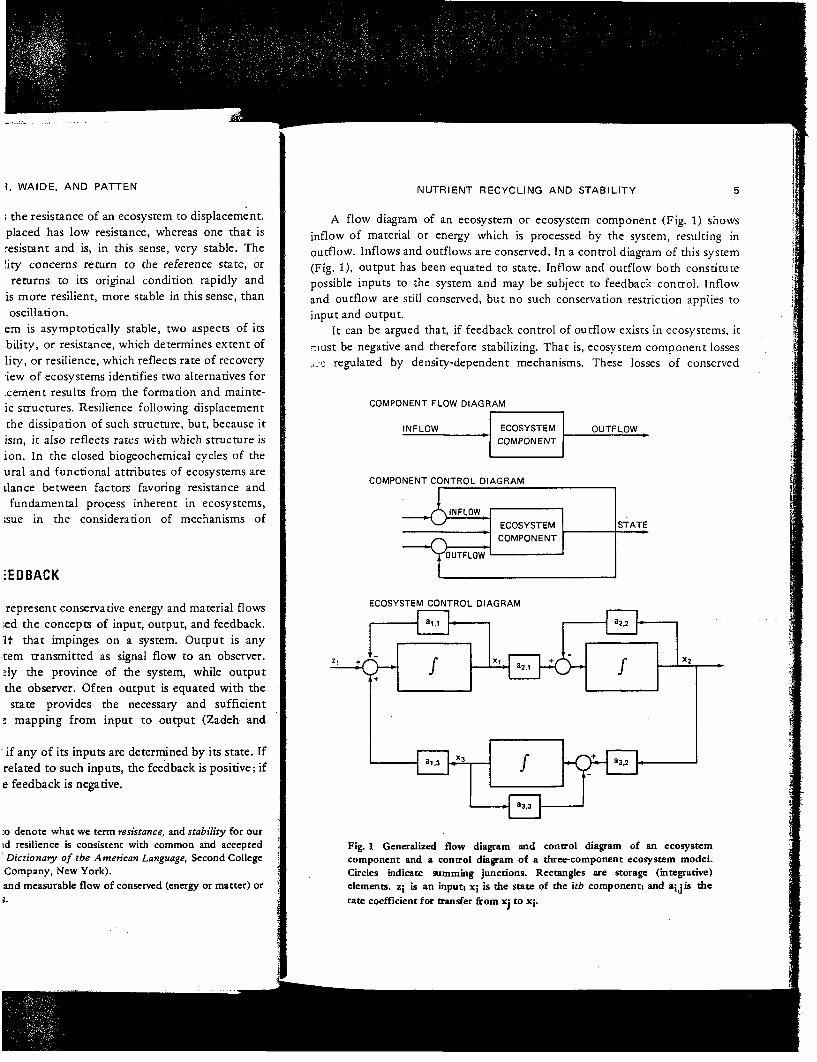
A flow diagram of an ecosystem or ecosystem component (Fig. 1) showsinflow of material or energy which is processed by the system, resulting inoutflow. Inflows and outflows are conserved. In a control diagram of this system(Fig. 1), output has been equated to state. Inflow and outflow both constitutepossible inputs to the system and may be subject to feedback control. Inflowand outflow are still conserved, but no such conservation restriction applies toinput and output.

It can be argued that, if feedback control of outflow exists in ecosystems, itmust be negative and therefore stabilizing. That is, ecosystem component lossesare regulated by density-dependent mechanisms. These losses of conserved

COMPONENT FLOW DIAGRAM

INFLOW

COMPONENT CONTROL DIAGRAM

ECOSYSTEM CONTROL DIAGRAM

Fig. 1 Generalized flow diagram and control diagram of an ecosystemcomponent and a control diagram of a three-component ecosystem model.Circles indicate summing junctions. Rectangles are storage (integrative)elements, z; is an input; x; is the state of the \tb component; and a; ;is therate coefficient for transfer from x: to xj.


quantities must be offset by inflows to maintain nonzero states. At the organismand population levels, positive-feedback mechanisms operate to promote inflowand are therefore potentially destabilizing (Milsum, 1968). Mobilization ofresources is the essence of life processes (Smith, 1972); however, manydensity-dependent mechanisms exist which regulate inflow in a negative-feedback sense (Whittaker and Woodwell, 1972). Further, a macroscopicperspective leads to the conclusion that ecosystems and their components areultimately resource limited (Hairston, Smith, and Slobodkin, I960; Wiegert andOwen, 1971; Patten et al., 1974; Waide and Webster, 1975; Webster and Waide,1975). Under unperturbed conditions ecosystems are maximally expandedwithin the resource hyperspace to the point of kinetic limitation of materialtransfers as set by the physicochemical environment (Blackburn, 1973). Thusinflow is limited by matter-recycling kinetics that ensure boundedness. Boundedinflow and negative-feedback control of outflow coupled with the first law ofthermodynamics (mass conservation) form the basis of our argument fornonzero ecosystem states that are stable.

These ideas lead to a representation of ecosystems (Fig. 1) as sets ofinteracting components, each regulated by a negative-feedback loop related to itsdissipative (i.e., turnover) character. Material recycling is displayed as feedbackinvolving multiple system components. Because material flow is involved,recycling must be interpreted as positive feedback (H. T. Odum, 1971). Thispoint emphasizes a fundamental difference between feedback in a controldiagram and material recycling in a flow diagram. In the control diagram controlis mediated by nonconservative information flows, whereas in the flow diagramcontrol among components is exerted only through material or energy flows thatmust be conserved. Feedback mechanisms are not explicit in flow diagrams butmust, nevertheless, be incorporated into any mathematical model of the system.

Thus a systems theoretic interpretation of nutrient cycling as feedback leadsto the general conclusions already elaborated: (1) biotic tendency for unlimitedgrowth is bounded by the first law of thermodynamics (mass conservation), asmediated through material-recycling kinetics and (2) negative-feedback decay toabiotic physicochemical equilibrium, if material and energy inflows are removed,is assured by the dissipative character of ecosystems and the second law ofthermodynamics. The first conclusion guarantees Liapunov stability. The twoconclusions together are sufficient to establish the stability of nonzeroecosystem trajectories (Patten, 1974).

MEASURES OF RELATIVE STABILITY

The General Linear Ecosystem Model

The dynamics of conserved quantities in an ecosystem with n componentscan be described mathematically as

WAIDE, AND PATTEN

vs to maintain nonzero states. At the organismdback mechanisms operate to promote inflow:stabilizing (Milsum, 1968). Mobilization of: processes (Smith, 1972); however, many:xist which regulate inflow in a negarive-Woodwell, 1972). Further, a macroscopic

an that ecosystems and their components areton, Smith, and Slobodkin, I960; Wiegert andWaide and Webster, 1975; Webster and Waide,iitions ecosystems are maximally expanded:o the point of kinetic limitation of materialicmical environment (Blackburn, 1973). Thusing kinetics that ensure boundedness. Boundeditrol of outflow coupled with the first law of.tion) form the basis of our argument forstable.rsentation of ecosystems (Fig. 1) as sets ofilated by a negative-feedback loop related to its:er. Material recycling is displayed as feedbackponents. Because material flow is involved,; positive feedback (H. T. Odum, 1971). Thisi.l difference between feedback in a controla flow diagram. In the control diagram control

nformation flows, whereas in the flow diagramrted only through material or energy flows that•chanisms are not explicit in flow diagrams but:ed into any mathematical model of the system,irpretarion of nutrient cycling as feedback leads|y elaborated: (1) biotic tendency for unlimitedaw of thermodynamics (mass conservation), as.ing kinetics and (2) negative-feedback decay toum, if material and energy inflows are removed,laracter of ecosystems and the second law oflusion guarantees Liapunov stability. The twocient to establish the stability of nonzero?74).

ABILITY

odel

quantities in an ecosystem with n componentsas

N U T R I E N T RECYCLING AND STABILITY

x; = inflow — outflow (i = 1, 2, . . . , n)

7

(1)

Inflow can emanate from outside the ecosystem (z,) or from other systemcomponents (Fy, j = 1, 2 , . . . , n ; j =£ i). Outflow may pass to other components( F ; j ) or out of the system (F0i;). Hence Eq. 1 may be reformulated incompartmental form as

- ( F o i + L F : J )J l n) (2)

Material transfers within the ecosystem represent inflows to somecomponents and outflows from others. On the basis of the arguments givenabove and elsewhere (Patten et al., 1974; Webster and Waide, 1975), theseinternal flows, as well as outflows from the system, can be modeled asdonor-based according to the equation

"* • ~ 3 " • V'lj llj J

If we define component turnover rates as

a; ; = - L a; ; - a0 j (i = 1, 2, . . . , n)

Eq. 2 becomes

x; = Z + ( i= 1, 2 , . . . , n )

(3)

(4)

(5)

Because all x; and F;j represent material or energy, they must be nonnegative,which ensures that

Equation 5 can be expressed in matrix form as

x = Ax + z

(6)

(7)

where x is the state vector, z is the input vector, and A is a matrix of (possiblytime dependent) rate coefficients defined by Eq. 3. The mathematical con-straints defined in Eqs. 4 to 6 are sufficient to guarantee the asymptotic stabilityof this model (Hearon, 1953, 1963). In addition, the model is sufficient forsimulating nominal and small displacement dynamics of ecosystems (e!g., Olson,1^63; Patten, 1972; Patten et al., 1974). Implicit within the model structure".ietined by Eqs. 1 to 7 are both accumulative and dissipative tendencies; thusthis model is useful for examining macroscopic questions of ecosystem relativestability.

WEBSTER, WAIDE, AND PATTEN

rtfA-Order Measures

The system defined by Eq. 7 is an nfA-order system, being composed of nfirst-order equations. Relative stability indexes can be derived for this system.Specifically, the characteristic roots or eigenvalues of the system defined byEq. 7, denoted \k (k = 1, 2,. .. , n), can be found by solving the matrixequation

det (XI - A) = 0 (8)

where det denotes the determinant of the indicated matrix, and I is the n X nidentity matrix. The solution to Eq. 7 can be expressed in terms of thesecharacteristic roots, where each eigenvalue defines a particular mode of systembehavior, as

k=l(9)

where c^ is a constant, b^ is the eigenvector associated with the eigenvalue \k,and p is a particular solution to Eq. 7 determined by z.

Clearly, if any X^ > 0, the system will grow exponentially. According to atheorem attributed to Liapunov and Poincare (Bellman, 1968), a system isasymptotically stable if all the characteristic roots have negative real parts.

Two relative stability measures may be derived from these n eigenvalues. Thefirst is the critical root, defined as the characteristic root with the smallestabsolute value (Funderlic and Heath, 1971). Given that the system isasymptotically stable, the critical root is the one most likely to become positive.Hence this index indicates the system's margin of stability. This critical root isthe smallest turnover rate (the longest time constant) in the system. Thus thesystem does not recover fully from displacement until this slowest component ofthe transient response decays away. Second, the trace of the matrix A (the sumof the diagonal elements) relates to the response time following perturbation(Makridakis and Weintraub, 1971b). Since the sum of the main diagonal;elements of A equals the sum of the eigenvalues, we have used the mean root,defined as the mean value of the n eigenvalues, as an equivalent measure ofresponse time. The mean root reflects the time required for most of the system, \or for some hypothetical mean component of the system, to recover following;displacement.

Second-Order Measures

Extensive experience in control-systems engineering has demonstrated thejutility of approximating higher order linear systems as second order forfanalytical purposes (DiStefano, Stubberud, and Williams, 1967; Shinners, 1972).|Child and Shugart (1972) provided a rationale for implementing such an|

AND PATTEN

Border system, being composed of nlexes can be derived for this system,igenvalues of the system defined byi be found by solving the matrix

0 = 0 (8)

: indicated matrix, and I is the n X ncan be expressed in terms of thesedefines a particular mode of system

;xk< + P (9)

or associated with the eigenvalue A^,mined by z.

1 grow exponentially. According to ancare (Bellman, 1968), a system isc roots have negative real parts.derived from these n eigenvalues. Thecharacteristic root with the smallest1971). Given that the system is

ic one most likely to become positive.argin of stability. This critical root isime constant) in the system. Thus the:ment until this slowest component of;id, the trace of the matrix A (the sumresponse time following perturbationnee the sum of the main diagonalnvalues, we have used the mean root,nvalues, as an equivalent measure oftime required for most of the system,

it of the system, to recover following

ns engineering has demonstrated thei linear systems as second order fori, and Williams, 1967; Shinners, 1972).rationale for implementing such an


approach in studying ecosystem behavior and applied it to an analysis ofmagnesium cycling in a tropical forest. Waide et al. (1974) used this approach inanalyzing a model of calcium dynamics in a temperate forest. Hubbell (1973a, b)demonstrated the benefits of a frequency-domain analysis of second-orderpopulation models.

In this approach the behavior of an nth-order system of the form of Eq. 7 isapproximated as second order with the equation

(10)

where f is the damping ratio and cjn is the undamped natural frequency(DiStefano et al., 1967). The characteristic roots of this equation are given by

The roots of this second-order approximation represent the apparent roots ofthe original nth-order system. That is, these two eigenvalues, as well as thenatural frequency, represent weighted mean roots of the higher order system.They capture most of the information contained in the nth-order trajectories.The weighting function that determines these second-order parameters from then original eigenvalues is related to the magnitude of the eigenvector componentsof the nth-order system (Eq. 9).

From Eq. 11, if f = 1, the system is said to be critically damped, the systemresponds rapidly and without oscillation following displacement, and X t ,X2 = —o;n. If f > 1, the system is overdamped, the response of the system isslower than that of a critically damped system, though still nonoscillatory, andthe eigenvalues are real and unequal. If f < 1, the system in underdamped, andthe roots are complex and are given by

^•l A2 = ~?wn ±Jcon (1 ~~ f 2 ) (12)i/

where j = (—1) . The response of such a system to displacement, though initiallymore rapid than a critically damped system, is oscillatory. If f = 0, the roots areimaginary, and wn is the radian frequency of oscillation. If f < 0, theeigenvalues have positive real parts, and the system is unstable.

Given that the system under study is asymptotically stable (i.e., f > 0), thetwo parameters wn and f may be used as measures of relative stability. Thenatural frequency wn measures (inversely) the resistance of the system todisplacement. A system with a large natural frequency is especially susceptible todisturbance, whereas a system with a small natural frequency strongly resistsdisplacement. Similarly the magnitude of the damping ratio ? indicates the rateof system response following displacement, the resilience of the system. If thesystem is overdamped, the return to steady state is monotonic but slow. Ifunderdamped, the system responds in an oscillatory fashion. A critically damped


system exhibits the most rapid response possible without oscillation and thus hasmaximum resilience.

In this paper we investigate- relationships between specific properties ofecosystem nutrient cycles and discuss the four above-mentioned relative stabilityindexes: critical root, mean root, natural frequency, and damping ratio. We taketwo approaches. The first is a stochastic approach, using Monte Carlotechniques. In the second approach we construct hypothetical ecosystem modelsbased on a characterization of alternative properties of nutrient cycles andinvestigate the relative stability of these models. We also provide furtherecological understanding of the four relative stability indexes and extend thebasis for their implementation. Attention is restricted to time-invariant systemsfor heuristic purposes.

STOCHASTIC APPROACH

Construction and analysis of random matrices was used successfully tofurther understanding of general system properties and to investigate effects ofspecific system characteristics (e.g., connectivity) on such system-level propertiesas stability (Ashby, 1952; Gardner and Ashby, 1970; Makridakis and Weinrraub,1971a, b; May, 1972, 1973; Makridakis and. Faucheux, 1973; Waide andWebster, 1975; Webster and Waide, 1975). We initially followed such anapproach to establish general relationships among relative stability indexes andsystem properties, focusing especially on the amount of recycling.

Methods

In constructing random matrices, off-diagonal elements a.-ltj, i ^ j , of the Amatrix (Eq. 7) were chosen from a specified statistical distribution (e.g., uniformon [0,1]). Rates of nutrient loss to the environment (ao,i) were chosen from thesame distribution and main diagonal elements calculated according to Eq. 4. Forsome analyses, off-diagonal elements were defined as nonzero according to aspecified probability of connectivity. Only a single input T.\ was used for allanalyses.

Following matrix construction, eigenvalues were calculated (Westley andWatts, 1970), and the critical root and mean root were determined. We alsocalculated an index of recycling (I) as the summed flows represented by theupper triangle divided by the input. That is, the ratio of nutrients recycled tonutrient input from the environment is

(13)

The synthetic division algorithm of Ba Hli (1971) was used to estimate thevalues of the natural frequency and damping ratio. A unit step input was applied

UDE, AND PATTEN NUTRIENT RECYCLING AND STABILITY 11

se possible without oscillation and thus has

ationships between specific properties ofthe four above-mentioned relative stability

ural frequency, and damping ratio. We takestochastic approach, using Monte Carlo/e construct hypothetical ecosystem models:rnative properties of nutrient cycles and" these models. We also provide furtherr relative stability indexes and extend thention is restricted to time-invariant systems

andom matrices was used successfully totern properties and to investigate effects ofonnectivity) on such system-level propertiesnd Ashby, 1970; Makridakis and Weintraub,ridakis and. Faucheux, 1973; Waide andle, 1975). We initially followed such anmships among relative stability indexes andf on the amount of recycling.

s, off-diagonal elements ajj, i^j, of the Apecified statistical distribution (e.g., uniformthe environment (ao,;) were chosen from the. elements calculated according to Eq. 4. Forts were defined as nonzero according to ay. Only a single input z t was used for all

eigenvalues were calculated (Westley and: and mean root were determined. We also) as the summed flows represented by thet. That is, the ratio of nutrients recycled totis

n of Ba Hli (1971) was used to estimate thedamping ratio. A unit step input was applied

to each randomly constructed matrix to generate the required discreteinput—output time series. Synthetic division yielded the coefficients of a generalsecond-order transfer function, which were equated with coefficients of thespecific transfer function of Eq. 10, allowing estimation of the natural frequencyand damping ratio (Hill, 1973).

The above process was repeated 50 or 100 times for each type of matrixconstructed. The resulting sets of values were subjected to linear regressionanalysis to determine the presence of significant relationships among calculatedvariables. To ensure that results were not biased by methods of matrixconstruction, we analyzed a variety of matrices of three sizes (n = 4, 6, 10). Invarious experiments, matrix elements were sampled from uniform distributionsof different ranges and from normal distributions with various means andvariances. We tried a wide range of upper and lower triangle connectivity, andselected several different outputs for use in the synthetic division. In some casesmodifications were made to obtain a pyramid-type structure of compartmentalstanding crops. We also examined results of increased input and recycling.

Results

The following trends were generally observed across the range of matricesanalyzed. Increases in the amount of recycling relative to input led to increasesin the critical root (moved closer to zero), decreases in the mean root (movedfarther from zero), and decreases in the natural frequency. Also, larger criticaland mean roots were both associated with smaller natural frequencies.

Trends in the damping ratio initially appeared to be variable. In some cases ftended to decrease with increasing recycling, critical root, and mean root. Inother cases f showed the opposite behavior. Closer inspection revealed that, inthe first case, all systems were underdamped, whereas in the second case theywere overdamped. Thus, when the quantity |1 — f | was considered, the resultswere unambiguous: |1 — fl increased with increasing values of recycling, criticalroot, and mean root.

DETERMINISTIC APPROACH

Our second approach to investigating relationships between material recy-cling and ecosystem stability involved construction and analysis of hypotheticalecosystem models. Two basic assumptions are inherent in these analyses: (1)ecosystems are units of selection and evolve from systems of lower selectivevalue to ones of higher selective value (we are not invoking any superorganismconcept; this evolution is accomplished through species coevolution) (Slobodkin,1964; Darnell, 1970; Lewontin, 1970; Dunbar, 1972; Whittaker and Woodwell,1972; Blackburn, 1973); (2) those ecosystems with highest selective value areones which optimize utilization of essential resources. Exceptions to the

IN


selection for ecosystems geared to efficient resource utilization would existwhere resources were extremely abundant or where the system as a whole wasoperating under other environmental stress (Odum, 1967; Waide et al., 1974).An example might be a stream which receives krge allochthonous inputs ofdetritus and which is strongly influenced by current action. In other ecosystemsselective value involves efficient conservation and recycling of essential nutrients.

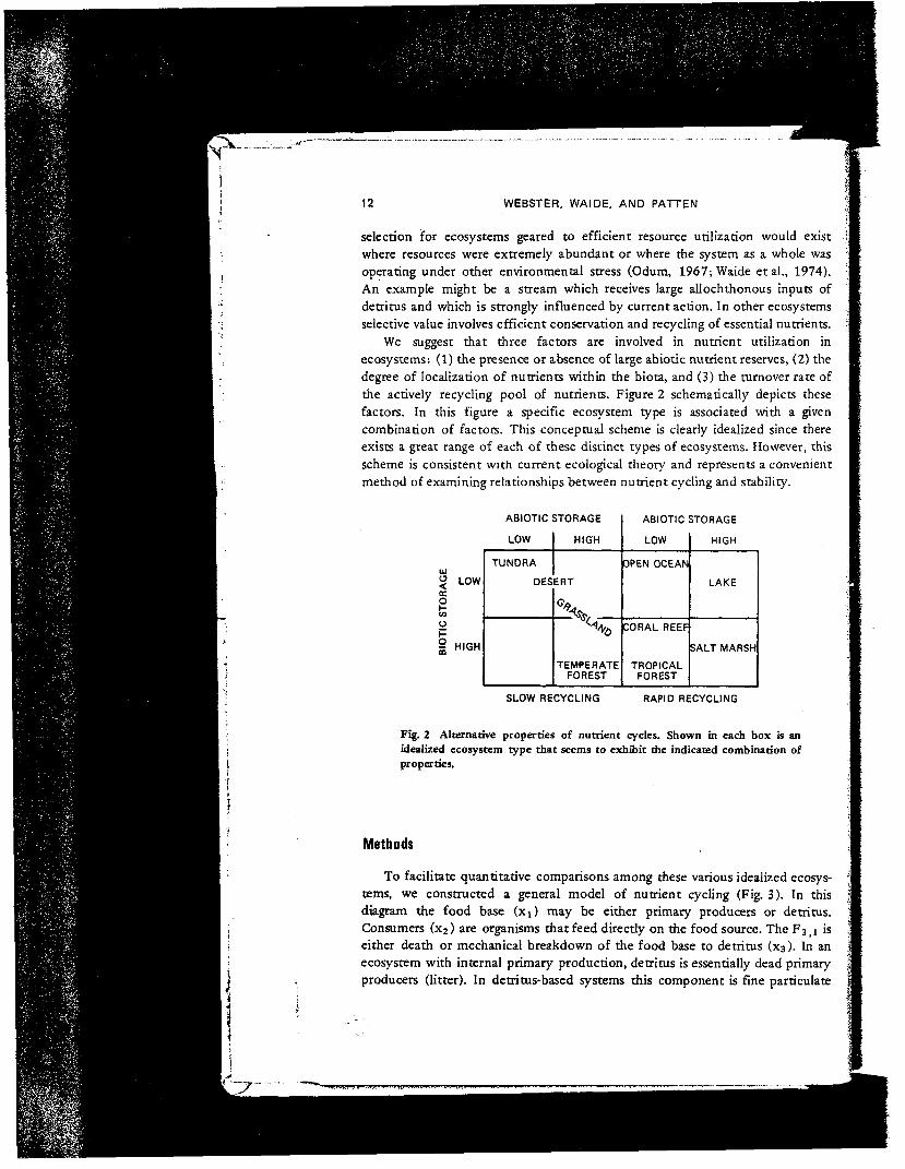
We suggest that three factors are involved in nutrient utilization inecosystems: (1) the presence or absence of large abiotic nutrient reserves, (2) thedegree of localization of nutrients within the biota, and (3) the turnover rate ofthe actively recycling pool of nutrients. Figure 2 schematically depicts thesefactors. In this figure a specific ecosystem type is associated with a givencombination of factors. This conceptual scheme is clearly idealized since thereexists a great range of each of these distinct types of ecosystems. However, thisscheme is consistent with current ecological theory and represents a convenientmethod of examining relationships between nutrient cycling and stability.

ABIOTIC STORAGE

UJ« LOW1CO

ot-i HIGH

LOW

TUNDRADES

HIGH

= RT

^TEMPERATE

FOREST

ABIOTIC STORAGELOW

OPEN OCEAN

CORAL REEF

TROPICALFOREST

HIGH

LAKE

SALT MARSH

SLOW RECYCLING RAPID RECYCLING

Fig. 2 Alternative properties of nutrient cycles. Shown in each box is anidealized ecosystem type that seems to exhibit the indicated combination ofproperties.

Methods

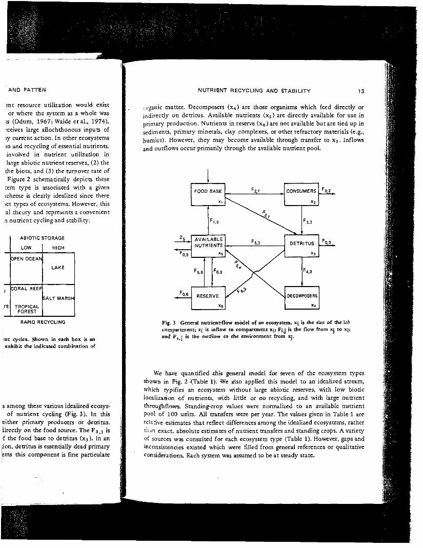
To facilitate quantitative comparisons among these various idealized ecosys-tems, we constructed a general model of nutrient cycling (Fig. 3). In thisdiagram the food base (xj) may be either primary producers or detritus.Consumers (x2) are organisms that feed directly on the food source. The F3 i l iseither death or mechanical breakdown of the food base to detritus (xs). In anecosystem with internal primary production, detritus is essentially dead primaryproducers (litter). In detritus-based systems this component is fine particulate

AND PATTEN NUTRIENT RECYCLING AND STABILITY 13

organic matter. Decomposers (x4) are those organisms which feed directly orindirectly on detritus. Available nutrients (xs) are directly available for use inprimary production. Nutrients in reserve (x6) are not available but are tied up insediments, primary minerals, clay complexes, or other refractory materials (e.g.,humics). However, they may become available through transfer to xs. Inflowsand outflows occur primarily through the available nutrient pool.

)

FE

ABIOTIC STORAGELOW

OPEN OCEAN

CORAL REEF

TROPICALFOREST

HIGH

LAKE

SALT MARSH

RAPID RECYCLING

ro.2

"•0,3.

Fig. 3 General nutrient-flow model of an ecosystem, x; is the size of the \thcompartment; z; is inflow to compartment xjj Fj; is the flow from x: to x;;and Fn i is the outflow to the environment from x;.o»J J

s among these various idealized ecosys-of nutrient cycling (Fig. 3). In this

either primary producers or detritus,directly on the food source. The F3>1 is|f the food base to detritus (x3). In an|ion, detritus is essentially dead primaryems this component is fine paniculate

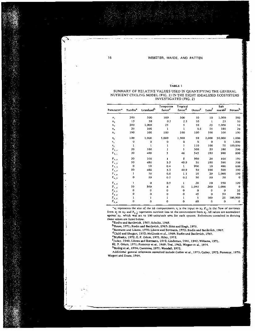
We have quantified .this general medel for seven of the ecosystem typesshown in Fig. 2 -(Table 1). We aiso applied this model to an idealized stream,which typifies an ecosystem without large abiotic reserves, with low bioticlocalization of nutrients, with little or no recycling, and with large nutrientthroughflows. Standing-crop values were normalized to an available nutrientpool of 100 units. All transfers were per year. The values given in Table 1 arerelative estimates that reflect differences among the idealized ecosystems, rathert-an exact, absolute estimates of nutrient transfers and standing crops. A varietyof sources was consulted for each ecosystem type (Table 1). However, gaps andinconsistencies existed which were filled from general references or qualitativeconsiderations. Each system was assumed to be at steady state.


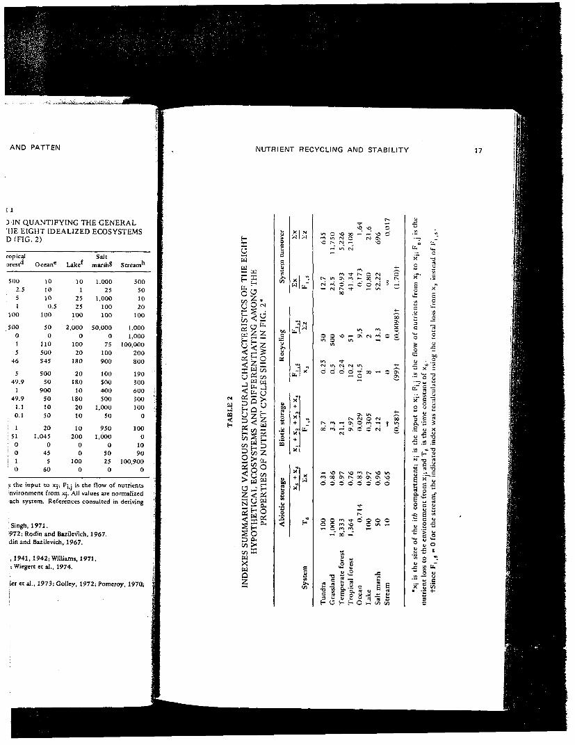
From these numbers we derived several indexes which reflect structuralcharacteristics of the eight ecosystems and which quantify the concepts ofabiotic storage, biotic storage, and recycling (Table 2). Both the turnover time ofthe reserve (T6 = l/|a6i6|) and the proportion of nutrients localized in the twoabiotic pools [(xs + x6)/2x] are indexes of abiotic storage. Reserve turnovervaries from slow in forests to fast in oceans and streams. The proportion of totalnutrients in abiotic compartments is highest in temperate forests and lakes andlowest in tundra.

Biotic storage, given by the turnover time of biotic compartments[(KI + x2 + x3 + x 4 ) / F I j 5 ] , is higher in terrestrial ecosystems and lower inaquatic ecosystems.

We calculated two indexes of recycling. The turnover rate of the detrituspool (Fi i 5 /x 3 ) is higher in aquatic systems and generally lower in terrestrialecosystems, except for tropical forests where there is a rapid turnover ofdetritus. The ratio of recycling to input (F! ?5/2z), as used in stochastic analyses,is approximately the inverse of the other recycling index.'However, since systemswith larger biotic pools typically recycle more nutrients than do systems withsmaller biotic standing crops, this index partially confounds storage andrecycling. This index ranges from 500 for grasslands to 0 for streams.

Two other useful indexes are the ratios of total standing crop to recyclingmaterial (Sx/F l j S) and total standing crop to total inflow (Zx/2z). Bothindexes estimate system turnover time. Longest turnover times occur intemperate forests and grasslands, whereas there is rapid turnover in stream andocean ecosystems.

The specific values given in Table 1 have obvious deficiencies. Each idealizedecosystem represents a wide spectrum of actual ecosystems differing in manyimportant characteristics. Similarly the kinetics of specific nutrients within agiven ecosystem differ, quantitatively and qualitatively. In quantifying thegeneral model shown in Fig. 3, we have attempted to suppress such specificdetails and to focus instead on the alternative properties of nutrient cyclesdepicted in Fig. 2. Our emphasis is thus on macroscopic properties of ecosystemsrather than on specific differences between systems or nutrients. Comparison ofthe structural indexes (Table 2) with Fig. 2 reveals that the chosen values agreewell with the idealized conceptualization.

Results

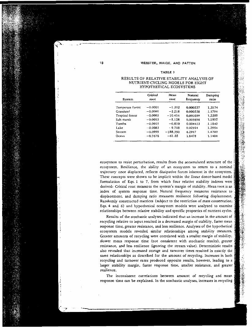
The eight models were analyzed in the same fashion as described previously,providing values for critical root, mean root, natural frequency, and dampingratio (Table 3). Both critical root and natural frequency were smallest (inabsolute value) for the temperate forest and grassland models and largest for thestream model and tended to be smaller (in absolute value) for the four terrestrialecosystem models. All values of damping were greater than 1, indicating all eightecosystem models to be overdamped. The smallest value was obtained for the

1

E, AND PATTEN

:veral indexes which reflect structuraland which quantify the concepts of

ing (Table 2). Both the turnover time of'ortion of nutrients localized in the twotes of abiotic storage. Reserve turnoverins and streams. The proportion of total;hest in temperate forests and lakes and

mover time of biotic compartmentsin terrestrial ecosystems and lower in

cling. The turnover rate of the detritusstems and generally lower in terrestrialts where there is a rapid turnover of(F! _ s /Sz), as used in stochastic analyses,r recycling index.'However, since systemscle more nutrients than do systems withindex partially confounds storage andir grasslands to 0 for streams.ratios of total standing crop to recyclingig crop to total inflow (2x/2z). Bothme. Longest turnover times occur insa.s there is rapid turnover in stream and

have obvious deficiencies. Each idealizedi of actual ecosystems differing in manyie kinetics of specific nutrients within af and qualitatively. In quantifying the^ave attempted to suppress such specificalternative properties of nutrient cycles

» on macroscopic properties of ecosystemsween systems or nutrients. Comparison ofrig. 2 reveals that the chosen values agreean.

n the same fashion as described previously,:an root, natural frequency, and dampingand natural frequency were smallest (in:st and grassland models and largest for the;r (in absolute value) for the four terrestrialling were greater than 1, indicating all eight1. The smallest value was obtained for the


ocean, the largest for the stream. No clear separation between terrestrial andaquatic ecosystems was obvious.

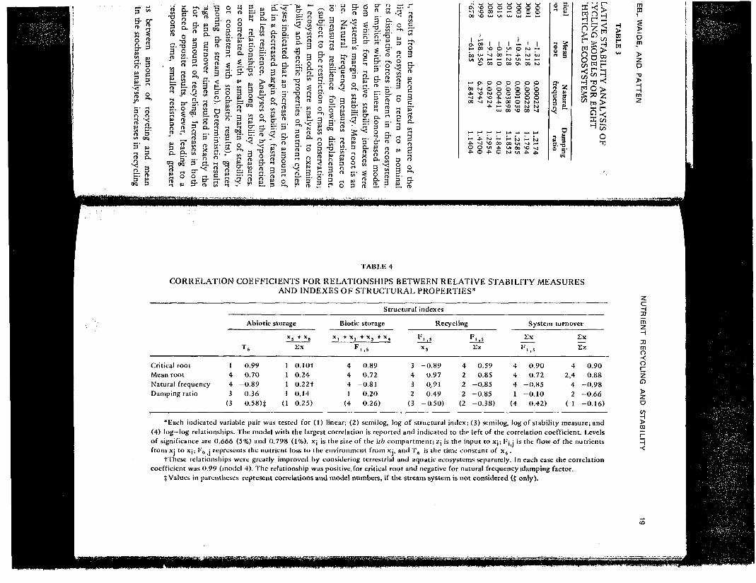
The relative stability indexes were then compared with the structural indexesgiven in Table 2, using least-squares regression. Correlation coefficients areshown in Table 4. Both critical and mean roots were directly related to theturnover time of the reserve nutrient pool T6, whereas the natural frequencyexhibited an inverse relationship. For longer turnover times, critical and meanroots were nearer zero, and the natural frequency was smaller.

Regressions against the proportion of nutrients in the two abiotic pools werenot significant However, when terrestrial and aquatic ecosystems were con-sidered separately, a trend was evident Increased abiotic storage or slowerabiotic turnover produced critical and mean roots nearer zero and smallernatural frequencies.

All four stability indexes were related to recycling. A greater recycling rate(Fi s/xa) or a smaller ratio of recycling to input (F1)5/Sz) resulted in rootsfarther from zero, a larger natural frequency, and greater damping.

Both critical and mean roots, as well as natural frequency, were significantlyrelated to system turnover (Sx/F l i5). All four indexes were correlated withturnover as related to system input (2x/Sz). In general, the slower the systemturnover rate (the greater the turnover time), the nearer the critical and meanroots were to zero, the smaller the natural trequency, and the smaller thedamping ratio.

The results clearly indicate that increased storage and turnover times(abiotic, biotic, or total), as well as increased amounts of recycling, lead tocritical and mean roots nearer zero and to smaller natural frequencies. Increasedrecycling and turnover rates (of biotic or abiotic elements, or their sum), on theother hand, lead to critical and mean roots that are farther from zero and tolarger natural frequencies. Relationships involving the damping ratio are lessclear. However, if we ignore the stream, which has no recycling (Fi iS = 0) andfor which the second-order approximation may not be accurate owing todominance by the extremely large nutrient inflow, other trends becomeapparent (Table 4). Although correlations are not as .large as for the otherstability indexes, damping generally tended to be directly related to storage orturnover times but inversely related to recycling or turnover rates. Thus dampingand natural frequency typically showed opposite behavior relative to thestructural indexes considered.

DISCUSSION

The preceding arguments were presented for the asymptotic stability ofecosystems. This stability is guaranteed by limitations on resource mobilizationand by the dissipative character of ecosystems. Resistance, the ability of an


TABLE 1SUMMARY OF RELATIVE VALUES USED IN QUANTIFYING THE GENERAL

NUTRIENT CYCLING MODEL (FIG. 3) IN THE EIGHT IDEALIZED ECOSYSTEMSINVESTIGATED (FIG. 2)

Parameter* Tundraa Grassland*5Temperate

forestcTropicalforestd Ocean6 Lakef

Saltmarsh£ Stream"

20015

20020

100100

01

203020500

50101

500010

50050

1,000100100

1,00001

10040010048010

48010100

5000010

1000.5

251

1005,000

011515.50.45.50.60.10.560010

5002.551

1001.500

015

465

49.91

49.91.10.11

510010

1010100.5

100500

110500545500

50900

50105020

1,0450

455

60

101

2525

1002,000

010020

18020

18010

180201010

20000

1000

1,00025

1,000100100

50,0000

75100900100500400500

1,00050

9501,000

050250

500501020

1001,0001,000

100.000200800190300600300100

0100

01090

100,9000

*x| represents the size of the \th compartment; Zj is the input to xj; Fj ; is the flow of nutrientsfrom xj to xj; and F0 ; represents nutrient loss to the environment from xj. All values are normalizedagainst X;, which was set to 100 units/unit area for each system. References consulted in derivingthese values are listed below.

"Rodin and Bazilevich, 1967; Schultz, 1969.-bReuss, 1971; Rodin and Bazilevich, 1967i Sims and Singh, 1971.

cBormann and Likens, 1970; Likens and Hermann, 1972; Rodin and Bazilevich, 1967.dChild and Shugart, 1972; McGinnis et al., 1969; Rodin and Bazilevich, 1967.eBrylinsky, 1972; E. P. Odum, 1971; Riley, 1972.fjuday, 194O; Ukens and Bormann, 1972; Undeman, 1941, 1942; Williams, 1971.BE. P. Odum, 1971; Pomeroy et al., 1969; Teal, 1962; Wiegert et al., 1974."Boling et a4., 1974; Cummins, 1971; Woodail, 1972. |Additional general references .consulted include Collier et al., 1973; Golley, 1972; Pomeroy, 1970; J

Wiegert and Evans, 1964.

AND PATTEN NUTRIENT RECYCLING AND STABILITY 17

D IN QUANTIFYING THE GENERAL'HE EIGHT IDEALIZED ECOSYSTEMSD(FIG. 2)

ropicaJorestd

5002.551

100500

015

465

49.91

49.9'•10.11

; si. 0! oi i

0

Ocean6

1010100.5

100500

110500545500

5090050105020

1,0450

455

60

Lakef

101

2525

1002,000

010020

18020

18010

180201010

20000

1000

SalemarshS

1,00025

1,000100100

50,0000

75100900100500400500

1,00050

9501,000

050250

Stream*1

500501020

1001,0001,000

100,000200800190300600300100

0100

01090

100,9000

s the input to Xj; Fj j is the flow of nutrientsnvironment from xj. All values are normalizedach system. References consulted in deriving

Singh, 1971.972; Rodin and Bazilevich, 1967.din and Bazilevich, 1967.

, 1941, 1942; Williams, 1971.; Wiegert et al., 1974.

ier et al., 1973; Goliey, 1972; Pomeroy, 1970;

t_*T"35rTl— wp g

O u

V) *

H 5 O

W Z Z*" r- u c s^^ i— V»'*^ ^ 3Hu *j vi^ CU 1^ [£< M

a §5>*J E~" O r ^9 ^? z zH ^ S

^ (/i "•*

co ^ D^ V3 ZO >« jV*^2 V3 /*• s?S oS tSU J H^ M 3« r °-1^ w 2S X

s5D ft<. en >UXwQZ

U>3

aCUVI

C/l*

50~X«5

U23M.ao£

u201.y_g<

5

xM

a?

«•X

X+«Xt.x"

x"+x"

^N

"1,T~

Nw

x"

vl

â,"

w

H°

£a>•»Crt

(^*o -o o

in •"* "O W —I — I \O "*r+i in (N O r*J C\ *^^c r^ M_ ^_ ô--» U1 (N

^_^ <*• £ C CM 3t * - m w ' \ i ' « i i - H 3 Q ( N ^

r-i " J O — i C O <N ° «-^ (N t^- •*• i— i m •— '

00Csin *^» O

^ 0 ^ " ^ U ^ ^ -

in rj-rg in (N fN »n ^^H O ^

O\ in ^-sC-* M O fN 00r s * m - ^ c s . o i ^ ' ™ ' g mM r o ^ g s O O ( N O

- H ^ O C - ^ O m t s . ' O mf n o O O \ r s M O \ C \ So o o o o o o o

2rÔ Q r ^ ' J ' O O O O

H" M" *

^^$ MO -u' o^ Si ^2 ^

^ c t. 15 Jj£• — Q^ .y c Ec ' : 3 £ r t " S J i | j Ss L y S ^ r t ^ i ;H U H H O » - J c / 5 c / 3

u~V) ^— , _"

0 M"1 "sX "O0 3

i vix .SS rto x

*2 2•i i3 ™c rt

'"X SO (-1O w

**- baj. _ CJZ. -o'^fl~ X 3•Is "§rV~ C —^- « 3i<" C "rtO ^JO -J U" r ••*3 .1 >.S u «

•S .2 .S.2 « "O^ T3 r".- c .iS 1 11 x~"S f - sQ. L- — •e t: 1s = "

- £ : £ « •« 2 - S! 1 10 „ 0" -C ||'53 o "I•£ So u« — U'I S .SX 5 00

Sac

18 WEBSTER^WAIOE, AND PATTEN

TABLE 3

RESULTS OF RELATIVE STABILITY ANALYSIS OFNUTRIENT-CYCLING MODELS FOR EIGHT

HYPOTHETICAL ECOSYSTEMS

System

Temperate forestGrasslandTropical forestSalt marshTundraLakeStreamOcean

Criticalroot

-0.0001-0.0001-0.0003-0.0013-0.0015-0.0083-0.0999-0.7678

Meanroot

-1.312-2.218

-10.456-5.128-0.810-9.718

-188.350-61.85

Naturalfrequency

0.0002270.0002280.0010390.0038980.0044130.029246.29471.8478

Dampingratio

1.21741.17941.25851.18521.18401.29541.47001.1404

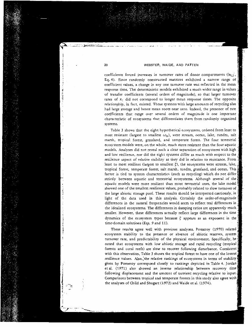
ecosystem to resist perturbation, results from the accumulated structure of theecosystem. Resilience, the ability of an ecosystem to return to a nominaltrajectory once displaced, reflects dissipative forces inherent in the ecosystem.These concepts were shown to be implicit within the linear donor-based modelformulation of Eqs. 1 to 7, from which four relative stability indexes werederived: Critical root measures the system's margin of stability. Mean root is anindex of system response time. Natural frequency measures resistance todisplacement, and damping ratio measures resilience following displacement.Randomly constructed matrices (subject to the restriction of mass conservation;Eqs. 4 and 6) and hypothetical ecosystem models were analyzed to examinerelationships between relative stability and specific properties of nutrient cycles.

Results of the stochastic analyses indicated that an increase in the amount ofrecycling relative to input resulted in a decreased margin of stability, faster meanresponse time, greater resistance, and less resilience. Analyses of the hypotheticalecosystem models revealed similar relationships among stability measures.Greater amounts of recycling were correlated with a smaller margin of stability,slower mean response time (not consistent with stochastic results), greaterresistance, and less resilience (ignoring the stream value). Deterministic resultsalso revealed that increased storage and turnover times resulted in exactly thesame relationships as described for the amount of recycling. Increases in bothrecycling and turnover rates produced opposite results, however, leading to alarger stability margin, faster response time, smaller resistance, and greaterresilience.

The inconsistent correlations between amount of recycling and meanresponse time can be explained. In the stochastic analyses, increases in recycling

7

O 00 O 00 O\ 00 N>

TABLE 4

CORRELATION COEFFICIENTS FOR RELATIONSHIPS BETWEEN RELATIVE STABILITY MEASURESAND INDEXES OF STRUCTURAL PROPERTIES*

Structural

Critical rootMean rootNatural frequencyDamping ratio

1443

(3

Abiotic

T6

0.990.70

-0.890.360.58)*

storageX

1111

(1

5 "*" X6Ex

o.iot0.240.22t0.140.25)

Biotic storage

X, + X

4441

(4

, + x 3 + x ,F.,S

0.890.72

-0.810.200.26)

3432

(3

indexes

RecyclingV, s

X3

-0.89-0.97

0.910.49

-0.50)

4222

(2

F ' ,sEz

0.590.85

-0.85-0.85-0.38)

System turnover

Ex Ex

4441

(4

F.,S

0.900.72

-0.85-0.10

0.42)

42,4

42

( 1

Ez

0.900.88

-0.98-0.66-0.16)

*liach indicated variable pair was tested for (1) linear; (2) semilog, log of structural index; (3) semilog, log of stability measure; and(4) log—log relationships. The model with the largest correlation is reported and indicated to the left of the correlation coefficient. Levelsof significance are 0.666 (5%) and 0.798 (1%). X| is the size of the ub compartment; Zj is the input to xj; l-'jj is the flow of the nutrientsfrom xj to xj ; !•'„ j represents the nutrient loss to the environment from xj, and T, is the time constant of x6.

t'l'liese relationships were greatly improved by considering terrestrial and aquatic ecosystems separately. In each case the correlationcoefficient was 0.99 (model 4). The relationship was positive for critical root and negative for natural frequency idamping factor.| Values in parentheses represent correlations and model numbers, if the stream system is not considered (f only).

.c2mZ

moo

o

CDF


coefficients forced increases in turnover rates of donor compartments (\a.\j\, ;Eq. 4). Since randomly constructed matrices exhibited a narrow range of |coefficient values, a change in any one turnover rate was reflected in the meanresponse time. The deterministic models exhibited a much wider range in valuesof transfer coefficients (several orders of magnitude), so that larger turnoverrates of x; did not correspond to longer mean response times. The oppositerelationship, in fact, existed. Those systems with large amounts of recycling alsohad large storage and hence mean roots near zero. Indeed, the presence of ratecoefficients that range over several orders of magnitude is one importantcharacteristic of ecosystems that differentiates them from randomly organizedsystems.

Table 3 shows that the eight hypothetical ecosystems, ordered from least tomost resistant (largest to smallest con), were stream, ocean, lake, tundra, saltmarsh, tropical forest, grassland, and temperate forest. The four terrestrialecosystem models were, on the whole, much more resistant than the four aquaticmodels. Analyses did not reveal such a clear separation of ecosystems with highand low resilience, nor did the eight systems differ as much with respect to theresilience aspect of relative stability as they did in relation to resistance. Fromleast to most resilient (largest to smallest f), the ecosystems were stream, lake,tropical forest, temperate forest, salt marsh, tundra, grassland, and ocean. This jfactor is tied to system characteristics (such as recycling) which do not differstrictly between aquatic and terrestrial ecosystems. Although several of theaquatic models were more resilient than most terrestrial ones, the lake model ]showed one of the smallest resilience values, probably related to slow turnover of ,the large abiotic storage pool. These results should be interpreted cautiously, in |light of the data used in this analysis. Certainly the order-of-magnitude |differences in the natural frequencies would seem to reflect real differences in 4the idealized ecosystems. The differences in damping ratios are apparently much *smaller. However, these differences actually reflect large differences in the time •dynamics of the ecosystem types because .f appears as an exponent in the •time-domain solutions (Eqs. 9 and 11). ij

These results agree well with previous analyses. Pomeroy (1970) related •ecosystem stability to the presence or absence of abiotic reserves, system |turnover rate, and predictability of the physical environment. Specifically, he|noted that ecosystems with low abiotic storage and rapid recycling (tropical |forests and coral reefs) are slow to recover following disturbance. Consistent:with this observation, Table 3 shows the tropical forest to have one of the lowest jresilience values. Also,jthe relative rankings of ecosystems in terms of stability!given by Pomeroy correspond closely to rankings depicted in Table 4. Jordanet al. (1971) also showed an inverse relationship between recovery timefollowing displacement and the amount of nutrient recycling relative to input.Comparisons between tropical and temperate forests in this study also agree withthe analyses of Child and Shugart (1972) and Waide et al. (1974).

)E, AND PATTEN NUTRIENT RECYCLING AND STABILITY 21

sr rates of donor compartments (la^jl ,natrices exhibited a narrow range ofturnover rate was reflected in the mean5 exhibited a much wider range in valuesof magnitude), so that larger turnover

ger mean response times. The oppositeems with large amounts of recycling alsonear zero. Indeed, the presence of rate

•rders of magnitude is one importantentiates them from randomly organized

netical ecosystems, ordered from least to, were stream, ocean, lake, tundra, salt

temperate forest. The four terrestrialluch more resistant than the four aquaticclear separation of ecosystems with highstems differ as much with respect to thethey did in relation to resistance. From;st f), the ecosystems were stream, lake,larsh, tundra, grassland, and ocean. This(such as recycling) which do not differ

il ecosystems. Although several of thein most terrestrial ones, the lake modelues, probably related to slow turnover ofsuits should be interpreted cautiously, inlysis. Certainly the order-of-magnitude.vould seem to reflect real differences ines in damping ratios are apparently muchaally reflect large differences in the time•ause f appears as an exponent in the

/ious analyses. Pomeroy (1970) relatedor absence of abiotic reserves, systeme physical environment. Specifically, hetic storage and rapid recycling (tropical:cover following disturbance. Consistent: tropical forest to have one of the lowestkings of ecosystems in terms of stabilityto rankings depicted in Table 4. Jordane relationship between recovery timeit of nutrient recycling relative to input.>erate forests in this study also agree with1) and Waideetai. (1974).

Inverse Relationships Between Resistanceand Resilience

Taken together our results indicate an inverse relationship between resistanceand resilience. Those factors which tend to increase resistance decreaseresilience, and those factors which increase resilience decrease resistance. Inaddition, those systems which are highly resistant have low resilience, and viceversa. Thus ecosystem evolution would seem to involve a compromise or balancebetween resistance and resilience. In some situations, selection has favoredecosystems with large storage and a large amount of recycling, factors thatconrribute to ecosystem persistence by increasing resistance to displacement.Other ecosystems in other environments have low storage and rapid recyclingand persist by responding rapidly following disturbance. The relationship is notan exact inverse, however. Results show, for example, the tropical forest to beboth less resistant and less resilient than either the temperate forest or grassland.Also, the grassland model is next to the most stable in terms of both resistanceand resilience, and the stream is least stable in both regards. Still, the notion of afunctional balance between ecosystem properties favoring resistance or resilienceis substantiated.

Environmental conditions that favor ecosystem resistance or resilience mustbe considered. In general, those environments in which resources are scarce orwh;,! place severe physicochemical limitations on resource mobilization willnot favor the accumulation of large biotic stores of nutrients. Systems thatrecycle nutrients rapidly, and hence are highly resilient, should be favored insuch environments. However, kinetic limitations on resource assimilation couldbe so severe as to produce systems that are neither resistant nor resilient, asstreams seem to be. On the other hand, environments in which resources areavailable and which place less severe limitations on resource mobilization shouldfavor the development of ecosystems that accumulate large nutrient reserves thatturn over slowly and hence are relatively more resistant. Such considerations inpart explain the separation between aquatic and terrestrial ecosystems in termsof resistance. With the exception of coral reefs, aquatic systems are generallylimited in their ability to retain and recycle essential resources (Pomeroy, 1970;Riley, 1972). Such systems are typically more resilient, and less resistant, thanterrestrial systems.

Also, as emphasized by Holling (1973), the balance between resistance andresilience is strongly influenced by the types of environmental fluctuationscommonly encountered by an ecosystem. For example, results suggest that thehypothetical ocean is the least resistant ecosystem next to the stream. It is notreasonable to expect selection for maximum resistance of such an ecosystemsince- the environment typically encountered by oceanic ecosystems is buffered(by me surrounding water mass) compared to that impinging upon a temperateforest, the most resistant ecosystem considered. Similar buffering is attained interrestrial ecosystems through large biotic storage.


As a corollary to these two last points, the kinds of environmental fluetuations an ecosystem "sees," and hence to which it responds, depend upon thedegree of resistance or resilience it exhibits. A system will filter out or attenuateinputs with a frequency greater than its natural frequency but will pass andhence react to inputs with a lower frequency. Thus analyses indicate thatterrestrial ecosystems are, on the average, currently responding to lowerfrequency environmental signals than are aquatic ecosystems. From the oppositeperspective, we could perhaps argue that higher frequency inputs may be moredamaging to terrestrial ecosystems and that selection has thus favored large,slowly recycling biotic structures that attenuate such persistent, potentiallydestabilizing inputs. Thus the degree of resistance or resilience a given ecosystemexhibits is determined by the types and frequencies of environmental fluctua-tions commonly encountered by the system, as well as by the environmentallimitations on resource mobilization which the system experiences.

Contribution of Component TurnoverRates to Stability

It was suggested above that one of the factors which characterizesecosystems is the presence of a large range in values of transfer rate coefficientsand turnover rates, typically over several orders of magnitude. Each componentturnover rate contributes to the resultant balance between resistance andresilience for a given ecosystem.

The concept of r and K selection define alternative evolutionary strategiesat the population level (Pianka, 1970, 1972). These ideas may be reformulatedin an ecosystem context by considering r selected species to be ones that haverapid turnover and low storage, thereby contributing to ecosystem resilience,whereas K specialists exhibit slow turnover and high storage, and thus contributeto resistance. Hence the degree of resistance or resilience observed in a givenecosystem results from the relative proportions of K and r selected components,respectively. This treatment does not seek to destroy the original meaning ofthese ideas but rather to suggest their implications for behavior at the ecosystemlevel.

During succession, ecosystems progress from stages that are relatively moreresilient to ones that are relatively more resistant. Although differing degrees of \environmental limitation and fluctuation will produce different balancesbetween resilience and resistance, all developmental processes involve someamount of biomass accretion and nutrient storage. However, even at steady state !a large variation in turnover rates of component populations is still present. It is jthe presence of such a variety of adaptations of component populations in :steady-state ecosystems which ensures their ability to respond followingdisturbance and hence which confers the property of resilience on ecosystems.For example, pin cherry is an early successional woody plant common inj

E, AND PATTEN

>ints, the kinds of environmental fluc-: to which it responds, depend upon theiits. A system will filter out or attenuatets natural frequency but will pass andrequency. Thus analyses indicate thaterage, currently responding to lower: aquatic ecosystems. From the oppositet higher frequency inputs may be moreI that selection has thus favored large,

attenuate such persistent, potentiallyresistance or resilience a given ecosystemd frequencies of environmental fluctua-^stem, as well as by the environmentalch the system experiences.

: of the factors which characterizesnge in values of transfer rate coefficientsil orders of magnitude. Each componentaltant balance between resistance and

lefine alternative evolutionary strategiesL972). These ideas may be reformulated ••!•J '-S5»I r selected species to be ones that have>y contributing to ecosystem resilience,ver and high storage, and thus contributestance or resilience observed in a givenportions of K and r selected components,seek to destroy the original meaning ofnplications for behavior at the ecosystem

press from stages that are relatively more•e resistant. Although differing degrees of .,ation will produce different balances. developmental processes involve some:nt storage. However, even at steady state>mponent populations is still present. It isjaptations of component populations in•es their ability to respond followingthe property of resilience on ecosystems.' successional woody plant common in


northeastern deciduous forests, which ensures their rapid return to steady-statefunction following major perturbation (Marks and Bormann, 1972; Marks,1974). Black locust seems to play a similar role in forest ecosystems in thesouthern Appalachians. Yet neither species is anything more than a minorcomponent of steady-state ecosystems in either locality. Clearly, their persis-tence within these ecosystems represents a system-level adaptation for resiliencewhich is not explained by considering dominant steady-state components alone.Similar examples could be cited for other ecosystem types.

The role of component turnover rates in regulating ecosystem stability is alsoemphasized by a consideration of the contribution of primary consumers toecosystem stability. Primary biophages are generally viewed as being able toregulate their rate of resource supply and hence the ability of a specificecosystem to accumulate biomass and store nutrients (Odum, 1962; Wiegert andOwen, 1971). Where environments favor ecosystem resistance, selection wouldthus seem to lead to mechanisms that suppress primary consumption, alle-lochemically, structurally, and via predators and parasites. However, in situationswhere ecosystem resilience is favored, mechanisms for reducing primaryconsumption would not necessarily be advantageous. Indeed, in such systemsherbivory would seem to be a major mechanism of nutrient regeneration andrecycling (Johannes, 1968; Pomeroy, 1970). Comparison of resilience values forthe eight hypothetical ecosystems investigated with estimates of the amount ofprimary production passing through primary biophages (Wiegert and Evans,1967; Wiegert and Owen, 1971; Golley, 1972) reveals a direct relationshipbetween these two parameters, with those ecosystem types in which primaryconsumption is higher typically being more resilient. Such a relationshipbetween herbivory and nutrient regeneration requires further experimentalverification, especially .in terrestrial ecosystems.

SUMMARY :

The theoretical perspective embodied in this paper represents an attempt toaccount for alternatives for persistence at the ecosystem level and at the sametime to relate ecosystem response to specific observable and measurableattributes of ecosystems. The argument that ecosystems are asymptoticallystable focuses attention on the critical area of relative stability. It clearlyidentifies two aspects '"of ecosystem relative stability, resistance and resilience.Resistance is related to the formation and maintenance of persistent ecosystemstructure. Resilience results from the tendencies inherent in ecosystems for theerosion of such structures. Thus this perspective offers to integrate various areasof ecological theory into a unified picture of ecosystem structure and function.Further research should help to establish the validity of these ideas. However, atpresent, they seem to represent a rigorous, operational approach to ecosystemtheory which is testable by both observation and experimental analysis. , v


ACKNOWLEDGMENTS

Research was supported in part by the Coweeta site of the EasternDeciduous Forest Biome, U. S. International Biological Program, funded by theNational Science Foundation under Interagency Agreement AG-199, 40-193-69with the Energy Research and Development Administration-Oak Ridge Na-tional Laboratory. This is paper No. 20, University of Georgia Contributions inEcosystems Ecology, We appreciate the helpful comments of R. V. O'Neill andR. G. Wiegert.

REFERENCES

Ashby, W. R., 1952, Design for a Brain, Chapman & Hall, Ltd., London.Ba Hli, F., 1971, A Time Domain Approach, in Aspects of Network and System Theory,

pp. 313-325, R. E. Kalman and N. DeCIaris (Eds.), Holt, Rinehart, and Winston, Inc.,New York.

Bellman, R. E., 1968, Some Vistas of Modern Mathematics: Dynamic Programming,Invariant Imbedding, and the Mathematical Biosciences, University of Kentucky Press,Lexington.

Blackburn, T. R., 1973, Information and the Ecology of Scholars, Science, 181: 1141-1146.Boling, R. H., Jr., R. C. Peterson, and K. W. Cummins, 1974, Ecosystem Modeling for Small

Woodland Streams, in Systems Analysis and Simulation in Ecology, Vol. 3, pp. 183-204,B. C. Patten (Ed.), Academic Press, Inc., New York.

Bormann, F. H., and G. E. Likens, 1970, The Nutrient Cycles of an Ecosystem, Sci. /\mer.,220= 92-101.

Brylinsky, M., 1972, Steady-State Sensitivity Analysis of Energy Flow in a MarineEcosystem, in Systems Analysis and Simulation in Ecology, Vol. 2, pp. 81-101, B.C.Parren (Ed.), Academic Press, Inc., New York.

Child, G. I., and H. H. Shugart, Jr., 1972, Frequency Response Analysis of MagnesiumCycling in a Tropical Forest Ecosystem, in Systems Analysis and Simulation in Ecology,Vol. 2, pp. 103-135, B. C. Patten (Ed.), Academic Press, Inc., New York.

Collier, B. D., G. W. Cox, A. W. Johnson, and P. C. Miller, 1973, Dynamic ecology,Prentice-Hall, Inc., Englewood Cliffs, N. J.

Cummins, K. W., 1971, Predicting Variations in Energy Flow Through a SemicontrolledLode Ecosystem, Michigan State University, Institute of Water Research, TechnicalReport 19, pp. 1-21.

Darnell, R. M., 1970, Evolution and the Ecosystem, Amer. Zool., 10: 9-16.DiStefano, J. J., A. K. Stubberud, and I. J. Williams, 1967, Feedback and Control Systems,

McGraw-Hill Book Company, New York.Dunbar, M. J., 1972, The Ecosystem as a Unit of Natural Selection, Trans. Conn. Acad. Arts

Sci., 44: 111-130.Funderlic, R. F., and M. T. Heath, 1971, Linear Compartmental Analysis of Ecosystems,

USAEC Report ORNL-IBP-71-4, Oak Ridge National Laboratory.Gardner, M. R., and W. R. Ashby, 1970, Connectedness of Large Dynamic (Cybernetic)

Systems: Critical Value of Stability, Nature, 228: 784.Golley, F. B., 1972, Energy Flux in Ecosystems, in Ecosystem Structure and Function,

pp. 69-90, J. A. Wiens (Ed.), Oregon State University Press, Corvallis.Hairston, N. G. F. E. Smith, and L. B. Slobodkin, I960, Community Structure, Population

Control, and Competition, Amer. Natur., 94: 421-425.

/AIDE, AND PATTEN

irt by the Coweeta site of the Easternnational Biological Program, funded by theInteragency Agreement AG-199, 40-193-69'elopment Administration-Oak Ridge Na-20, University of Georgia Contributions in

the helpful comments of R. V. O'Neill and

lapman & Hall, Ltd., London.iach, in Aspects of Network and System Theory,;Claris (Eds.), Holt, Rinehart, and Winston, Inc.,

Modern Mathematics: Dynamic Programming,\atical Biosciences, University of Kentucky Press,

he Ecology of Scholars, Science, 181: 1141-1146.V. Cummins, 1974, Ecosystem Modeling for Smallx and Simulation in Ecology, Vol. 3, pp. 183-204,., New York.The Nutrient Cycles of an Ecosystem, Sci. /inter.,

iidvity Analysis of Energy Flow in a MarineSimulation in Ecology, Vol. 2, pp. 81-101, B.C./ York.'2, Frequency Response Analysis of Magnesiumi, in Systems Analysis and Simulation in Ecology,, Academic Press, Inc., New York.on, and P. C. Miller, 1973, Dynamic neology,'...].ions in Energy Flow Through a Semicontrolledvercity, Institute of Water Research, Technical

osystem, Amer. Zoo/., 10: 9-16. •'-''•'. Williams, 1967, Feedback and Control Systems,k. : !;.-:..nit of Natural Selection, Trans. Conn. A cad. Arts

Linear Compartmental Analysis of Ecosystems,.idge National Laboratory.Connectedness of Large Dynamic (Cybernetic)

ture, 228: 784. ,.systems, in Ecosystem Structure and Function,ite University Press, Corvallis. ' -bodkin, 1960, Community Structure, Population'., 94: 421-425. * J^' ' ' ' ~l t n


Hearon, J. Z., 1963, Theorems on Linear Systems, Ann. N. Y. Acad. Sci., 108s 36-68..t 1953, The Kinetics of Linear Systems with Special Reference to Periodic Reactions,Bull. Math. Biophys., 15: 121-141.

Hill , J - i 'V, 1973, Component Description and Analysis of Environmental Systems, M.S.Thesis. Utah State University, Logan.

Holling, C. S., 1973, Resilience and Stability of Ecological Systems, Annu. Rev. Ecol. Syst.,4: 1-24. . .

Hubbell, S. P., 1973a, Populations and Simple Food Webs as Energy Filters, I. One-SpeciesSystems, Amer. Natur., 107: 94-121., 1973b. ibid, II. Two-Species Systems. Amer. Natur., 107: 122-151.

Hutchinson, G. E., 1948a, Circular Causal Systems in Ecology, Ann. N. Y. Acad. Sci., 50:221-246., 1948b, On Living in the Biosphere, Sci. Man., 67: 393-397.

Johannes, R. E., 1968, Nutrient Regeneration in Lakes and Oceans, in Advances inMicrobiology of the Sea, pp. 203-213, M. R. Droop and E. J. F. Wood (Eds.), AcademicPress, New York.

Jordan, F., J. R. Kline, and D. S. Sasscer, 1972, Relative Stability of Mineral Cycles inForest Ecosystems, Amer. Natur., 106: 237-253.

Juday, C., 1940, The Annual Energy Budget of an Inland Lake, Ecology, 21: 438-450.Lewontin, R. C., 1970a, The Meaning of Stability, in Diversity and Stability in Ecological

Systems, Symposia in Biology, No. 22, USAEC Report BNL-50175, BrookhavenNational Laboratory., 1970b, The Units of Selection, Annu. Rev. Ecol. Syst., 1: 1-18.

Liapunov, M. A., 1892, Probleme Generate de la Stabilite du Mouvement, Kharkov.Reprinted as Annals of Mathematical Study, No. 17, Princeton University Press,Princeton, N. J.

Likens, G. E., and F. H. Bormann, 1972, Nutrient Cycling in Ecosystems, in EcosystemStructure and Function, pp. 25-67, J. A. Wiens (Ed.), Oregon State University Press,Corvallis. ~~"

Lindeman, R. L., 1942, The Trophic-Dynamic Aspect of Ecology, Ecology, 23: 399-418., 1941, Seasonal Food-Cycle Dynamics in a Senescent Lake, Amer. Midland Natur., 26:636-673. . . . . . . .

MacArthur, R. H., 1955, Fluctuations of Animal Populations, and a Measure of CommunityStability, Ecology, 36: 533-536.

Makridakis, S., and C. Faucheux, 1973, Stability Properties of General Systems, Gen. Sys.,18=3-12. ,.., . . . . . , • ; . . . : . . • - , , : . ,, . . . ., and E. R. Weintraub, 1971a, On the Synthesis of General Systems, Parti, TheProbability of Stability, Gen. Sys., 16: 43-50., and E. R. Weintraub, 1971b, On the Synthesis of General Systems, Part II, OptimalSystem Size, Gen. Sys., 16: 51-54. ,. i

Marks, P. L., 1974, The Role of Pin Cherry (Prunuspennsyhanica L.) in the Maintenance ofStability in Northern Hardwood Ecosystem, Ecol. Monogr., 44: 73-88. : .-."..., and F. H. Bormann, 1972, Revegetation Following Forest Cutting: Mechanisms forReturn to Steady-State Nutrient Cycling, Science, 176: 914-915. ; - ..• 1. -'-.••:":: '-. .'.• ;•:?>•'••-:'

May, R. M., 1973, Stability and Complexity in Model Ecosystems, Princeton University- Press, Princeton,N. J. .;. , • ; „ ; < • ' • .-' .?:~ '•:•'•"'!-. ,' - • \ •• •• .:r r~ ; -•::•;•<.'.'-•-;•• \ ' •

• . 1972, Will a Large Complex System be Stable?, Nature, 238: 413-414. . .,,. ;McGinnis, J. T., F. B..Golley, R. G. Clements, G. I. Child, and M. J. Duever, 1969,

Elemental ^and_; Hydrologic Budgets of the Panamanian Tropical Moist Forest,BioScience, 19: 697-702. j ; • M .-1 , < - - • --'.-, '-

Milsum, J. H.,: 1968, Mathematical Introduction to General System Dynamics, in PositiveFeedback, pp. 23-65, J. H. Milsum (Ed.), Pergamon Press, New York. « ' , • - ; •

IV


Morowitz, H. J., 1966, Physical Background of Cycles in Biological Systems,/. Theor. Biol.:13: 60-62. •

Odum, E. P., 1971, Fundamentals of Ecology, W. B. Saunders Co., Philadelphia., 1969, The Strategy of Ecosystem Development, Science, 164; 262-270., 1962, Relationships Between Structure and Function in the Ecosystem, Jap. J. Ecol.:12: 108-118.

Odum, H. T., 1971, Environment, Power and Society, Wiley-Interscience, Inc., New York., 1967, Work Circuits and System Stress, in Primary Productivity and Mineral Cycling inNatural Ecosystems, pp. 81-138, H. E. Young (Ed.), University of Maine Press, Orono,Mafne.

Olson, J. S., 1963, Analog Computer Models for Movement of Nuclides ThroughEcosystems, in Radioecology, pp. 121-125, V. Shultz and A. W. Klements, Jr. (Eds.),Van Nostrand Reinhold Company, Cincinnati, and American Institute of Biological iSciences, Washington.

Patten, B. C., 1974, The Zero State and Ecosystem Stability, in Proceedings of the FirstInternational Congress of Ecology, Supplement. The Hague, Sept. 8—14, 1974, Centrefor Agricultural Publishing and Documentation, Wageningen., 1972, A Simulation of the Shortgrass Prairie Ecosystem, Simulation, 19: 177-186., D. A. Egloff, T. H. Richardson, and 38 Additional Coauthors, 1974, A TotalEcosystem Model for a Cove in Lake Texoma, Texas—Oklahoma, in Systems Analysisand Simulation in Ecology, Vol. 3, pp. 205-421, B. C. Patten (Ed.), Academic Press,Inc., New York.,and M. Witkamp, 1967, Systems Analysis of ' 34Cs Kinetics in Terrestrial Microcosms,Ecology, 48: 813-824.

Pianka, E. R., 1972, r and K Selection or b and d Selection? Amer. Natur., 106: 581-588., 1970, On r and K Selection, Amer. Natur., 102: 592-597.

Pomeroy, L. R., 1970, The Strategy of Mineral Cycling, Annu. Rev. Ecol. Syst., 1-. 171-190., R. E. Johannes, E. P. Odum, and B. Roffman, 1969, The Phosphorus and Zinc Cyclesand Productivity of a Salt Marsh, in Symposium on Radioecology, pp. 412-419,Proceedings of the Second National Symposium, May 15—17, 1967, D. J. Nelson andF. C. Evans (Eds.), Ann Arbor, Mich., USAEC Report CONF-670503.

Reuss, J. O., 1971, Soils of the Grassland Biome Sites, in Preliminary Analysis of Structureand Function in Grasslands, pp. 35-39, N. R. French (Ed.), Colorado State University,Fort Collins.

Riley, G. A., 1972, Patterns of Production in Marine Ecosystems, in Ecosystem Structureand Function, pp. 91-112, J. A. Wiens (Ed.), Oregon State University Press, Corvallis.

Rodin, L. E., and M. I. Bazilevich, 1967, Production and Mineral Cycling in TerrestrialVegetation, Oliver & Boyd, Edinburgh.

Schultz, A. M., 1969, A Study of an Ecosystem: The Arctic Tundra, in The EcosystemConcept in Natural Resource Management, pp. 77-93, G. M. VanDyne (Ed.), AcademicPress, Inc., New York.

Shinners, S. M., 1972, Modern Control System Theory and Application, Addison-WesleyPublishing Company, Inc., Reading, Mass.

Sims, P. L., and J. S. Singh, 1971, Herbage Dynamics and Net Primary Production in CertainUngrazed and Grazed Grasslands in North America, in Preliminary Analysis of Structureand Function in Grasslands, pp. 59-124, N. R. French (Ed.), Colorado State University,Fort Collins.

Slobodkin, L. B., 1964, The Strategy of Evolution, Amer. Sci., 52: 342-357.Smith, F. E., 1972, Spatial Heterogeneity, Stability, and Diversity in Ecosystems, Trans.

Conn. Acad. Arts Sci., 44: 309-335.Teal, J. M., 1962, Energy Flow in the Salt Marsh Ecosystem of Georgia, Ecology, 43:

614-624.


MD PATTEN

les in Biological Systems,;. Theor. BioL,

,f ' "Cs Kinetics in Terrestrial Microcosms,

Waide, J. B., J. E. Krebs, S. P. Clarkson, and E. M. Setzler, 1974, A Linear Systems Analysisof the Calcium Cycle in a Forested Watershed Ecosystem, in Progress in TheoreticalBiology, Vol. 3, pp. 261-345, R. Rosen and P.M. Snell (Eds.), Academic Press, Inc.,

New York.> and J. R- Webster, 1975, Engineering Systems Analysis: Applicability to Ecosystems,in Systems Analysis and Simulation m Ecology, Vol.4, B.C. Patten (Ed.), AcademicPress, Inc., New York (in press).

Webster, J. R., and J. B. Waide, 1975, Complexity, Resource Limitation, and the Stabilityof Ecosystems, in preparation.

Westley, G. W., and J. A. Watts, 1970, The Computing Technology Center NumericalAnalysis Library, Technical Report No. CTC-39, Oak Ridge National Laboratory.

Whittaker, R. H., and G. M. Woodwell, 1972, Evolution of Natural Communities, inEcosystem Structure and Function, pp. 137-159, J.A. Wiens (Ed.), Oregon StateUniversity Press, Corvallis.

Wiegert, R. G., R. R. Christian, ]. L. Gallagher, J. R. Hall, R. D. H. Jones, and R. L. Wetzel,1974, A Preliminary Ecosystem Model of Coastal Georgia Spartina Marsh, in RecentAdvances in Estuarine Research, J. Costlow (Ed.) (in press)., and F. C. Evans, 1967, Investigations of Secondary Productivity in Grasslands, inSecondary Productivity of Terrestrial Ecosystems, pp. 499-518, K. Petrusewicz (Ed.),Polish Academy of Science, Warsaw., and F. C. Evans, 1964, Primary Production and the Disappearance of Dead Vegetationon an Old Field in S. E. Michigan, Ecology, 45: 49-63., and D. F. Owen, 1971, Trophic Structure, Available Resources, and PopulationDensity in Terrestrial vs. Aquatic Ecosystems, J. Theor. Bio/., 30: 69-81.

Williams, R. B., 1971, Computer Simulation of Energy Flow in Cedar Bog Lake, Minnesota,Based on the Classical Studies of Lindeman, in Systems Analysis and Simulation inEcology, Vol. 1, pp. 543-582, B. C. Patten (Ed.), Academic Press, Inc., New York.

Woodall, W. R., Jr., 1972, Nutrient Pathways in Small Mountain Streams, Ph.D.Dissertation, University of Georgia, Athens.

Zadeh, L. A., and C. A. Desoer, 1963, Linear System Theory: The State Space Approach,McGraw-Hill Book Company, New York.

•m Theory and Application, 'Addison-Wesley

tion, Amer. Sci.- 52r342-357.;V V-^/:'^',liability, and Diversity m Ecosystems, Trans..:;

it Marsh Ecosystem ^^^Ecology,:43 =

conf-740513 proceedings of a symposium held at …coweeta.uga.edu/publications/279.pdf ·...

Documents