CONE CRUSHER MODELLING AND SIMULATION Development of a virtual rock crushing environment based on the discrete element method with industrial scale experiments for validation

Master of Science Thesis JOHANNES QUIST Department of Product and Production Development Division of product development CHALMERS UNIVERSITY OF TECHNOLOGY Göteborg, Sweden, 2012 Report No. 1652-9243

i

REPORT NO. 1652-9243

Cone Crusher Modelling and Simulation Development of a virtual rock crushing environment based on the discrete element

method with industrial scale experiments for validation

JOHANNES QUIST

Department of product and production development

CHALMERS UNIVERSITY OF TECHNOLOGY

Göteborg, Sweden 2012

ii

Cone Crusher Modelling and Simulation Development of a virtual rock crushing environment based on the discrete element method with industrial scale experiments for validation

JOHANNES QUIST

© JOHANNES QUIST, 2012

Technical report no. 1652-9243

Supervisor: Carl Magnus Evertsson, Professor

Department of Product and Production Development

Chalmers University of Technology

SE-412 96 Göteborg

Sweden

Telephone + 46 (0)31-772 1000

Cover. DEM simulation of a Svedala H6000 cone crusher studied in the thesis.

Repro service Göteborg, Sweden 2012

iii

Cone Crusher Modelling and Simulation Development of a virtual rock crushing environment based on the discrete element method with industrial scale experiments for validation JOHANNES QUIST

Department of Product and Production Development Chalmers University of Technology

SUMMARY

Compressive crushing has been proven to be the most energy efficient way of mechanically reducing the size of rock particles. Cone crushers utilize this mechanism and are the most widely used type of crusher for secondary and tertiary crushing stages in both the aggregate and mining industry. The cone crusher concept was developed in the early 20th century and the basic layout of the machine has not changed dramatically since then. Efforts aimed at developing the cone crusher concept further involve building expensive prototypes hence the changes made so far are incremental by nature.

The objective of this master thesis is to develop a virtual environment for simulating cone crusher performance. This will enable experiments and tests of virtual prototypes in early product development phases. It will also actualize simulation and provide further understanding of existing crushers in operation for e.g. optimization purposes.

The platform is based on the Discrete Element Method (DEM) which is a numerical technique for simulating behaviour of particle systems. The rock breakage mechanics are modelled using a bonded particle model (BPM) where spheres with a bi-modal size distribution are bonded together in a cluster shaped according to 3D scanned rock geometry. The strength of these virtual rock particles, denoted as meta-particles, has been calibrated using laboratory single particle breakage tests.

Industrial scale experiments have been conducted at the Kållered aggregate quarry owned by Jehander Sand & Grus AB. A Svedala H6000 crusher operating as a secondary crusher stage has been tested at five different close side settings (CSS). A new data acquisition system has been used for sampling the pressure and power draw sensor signals at 500 Hz. The crusher liner geometries were 3D-scanned in order to retrieve the correct worn liner profile for the DEM simulations.

Two DEM simulations have been performed where a quarter-section of the crusher is fed by a batch of feed particles. The first one at CSS 34 mm did not perform a good enough quality for comparison with experiments; hence a number of changes were made. The second simulation at CSS 50 mm was more successful and the performance corresponds well comparing with experiments in terms of pressure and throughput capacity.

A virtual crushing platform has been developed. The simulator has been calibrated and validated by industrial scale experiments. Further work needs to be done in order to post-process and calculate a product particle size distribution from the clusters still unbroken in the discharge region. It is also recommended to further develop the modelling procedure in order to reduce the simulation setup time.

Keywords: Cone Crusher, Discrete Element Method, Bonded Particle Model, Simulation, Numerical Modelling, Comminution, Rock breakage

iv

to Malin, Hanna & Helena

v

ACKNOWLEDGEMENT

I would like to acknowledge and thank a number of people that have made this work possible and worthwhile. First of all I appreciate all support and mentorship from my supervisor Magnus Evertsson and co-supervisor Erik Hulthén. Much appreciation goes to Gauti Asbjörnsson and Erik Åberg for helping out during the crusher experiments! Also, thank you Elisabeth Lee, Robert Johansson and Josefin Berntsson for help, support and fruitful discussions at the office!

Thanks to Roctim AB for initiating and supporting the project and for providing 3D scanning equipment! Special thanks to Erik and Kristoffer for helping with data collection on site!

I’m very grateful to Jehander Sand & Grus AB and all the operators for letting me conduct experiments at the Kållered Quarry and use the site laboratory. Special thanks to Michael Eriksson, Peter Martinsson and Niklas Osvaldsson!

Finally I would like to thank the engineering team at DEM-solutions Ltd for all the support, help and discussions. Special thanks to Senthil Arumugam, Mark Cook and Stephen Cole!

Johannes Quist

Göteborg, 2012

vi

NOMENCLATURE

BPM Bonded particle model DEM Discrete element method PBM Population balance model PSD Particle size distribution HPGR High pressure grinding roll CSS Close side setting OSS Open side setting DAQ Data acquisition CAD Computer aided design CAE Computer aided engineering CPUH CPU Processing Hours HMCM Hertz Mindlin Contact Model MDP Mechanical Design Parameter OCP Operational Control Parameter SOCP Semi-Operational Control Parameter OOP Operational Output Parameter SPB Single Particle Breakage IPB Interparticle breakage CRPS Chalmers Rock Processing Systems

Critical bond shear force Normal force

Critical bond normal force Tangential force

Shear bond stiffness Normal damping force

Normal bond stiffness

Tangential damping force J Bond beam moment of inertia Equivalent shear modulus Radius sphere A Equivalent young’s modulus Radius sphere B Equivalent radius Contact resultant force Equivalent mass Normal unit vector Normal overlap 𝑡 Tangential unit vector Tangential overlap Bond beam length Poisson ratio Bond disc radius Coefficient of restitution Bond resultant force Coefficient of static friction

Bond normal torque Normal stiffness

Bond shear torque Tangential stiffness s Eccentric throw Damping coefficient Eccentric speed DEM throughput capacity Mantle angular slip speed DEM mass flow

Chamber cross-sectional area Sectioning factor Mantle slope angle PSD scalping factor Estimated particle tensile strength

BPM bulk density Critical force for fracture Crushing force Hydrostatic bearing area

vii

TABLE OF CONTENTS 1. INTRODUCTION ............................................................................................................................................. 1

1.1 Background ............................................................................................................................................... 1

1.2 Objectives .................................................................................................................................................. 2

1.3 Research Questions .................................................................................................................................. 2

1.4 Deliverables ............................................................................................................................................... 2

1.5 Delimitations ............................................................................................................................................. 3

1.6 Thesis Structure ........................................................................................................................................ 3

1.7 Problem analysis ....................................................................................................................................... 4

2. THEORY ............................................................................................................................................................ 5

2.1 The Cone crusher ...................................................................................................................................... 5

2.1.1 Influence of parameters ..................................................................................................................... 7

2.1.2 Feeding conditions ............................................................................................................................. 9

2.1.3 Rock mass variation ........................................................................................................................ 10

2.2 The Discrete Element Method .............................................................................................................. 10

2.2.1 Approaches for modelling breakage .............................................................................................. 10

2.2.2 Previous work on DEM and crushing ........................................................................................... 11

2.2.3 Hertz-Mindlin Contact model ......................................................................................................... 11

2.2.4 Contact model calibration ............................................................................................................... 13

2.2.5 The Bonded Particle Model ............................................................................................................ 15

2.2.6 Future DEM capabilities ................................................................................................................. 16

2.3 Compressive breakage ........................................................................................................................... 17

2.3.1 Single Particle Breakage .................................................................................................................. 17

2.3.2 Inter Particle Breakage .................................................................................................................... 19

3. METHOD .......................................................................................................................................................... 20

3.1 DEM as a CAE tool ............................................................................................................................... 20

3.2 Bonded Particle Model Rock Population ............................................................................................ 20

3.2.1 Generating a bi-modal particle packing cluster ............................................................................. 21

3.2.2 Calibration of the bonded particle model ...................................................................................... 23

3.2.3 Introducing meta-particles by particle replacement ...................................................................... 23

3.3 Industrial scale crusher experiments ..................................................................................................... 24

3.4 Crusher geometry modelling ................................................................................................................. 27

3.5 Crusher data acquisition ........................................................................................................................ 29

4. CRUSHER EXPERIMENT ........................................................................................................................... 31

4.1 Size reduction .......................................................................................................................................... 31

4.2 Power draw .............................................................................................................................................. 32

4.3 Hydrostatic pressure ............................................................................................................................... 35

5. ROCK MATERIAL MODEL DEVELOPMENT ...................................................................................... 38

5.1 Single particle breakage experiment..................................................................................................... 38

5.2 BPM calibration ...................................................................................................................................... 40

5.2.1 Calibration simulations of BPMfine ................................................................................................ 40

5.2.2 Calibration simulations of BPMcoarse ............................................................................................. 42

6. CRUSHER SIMULATION ............................................................................................................................ 45

6.1 Particle Flow Behaviour ......................................................................................................................... 46

6.2 Breakage behaviour................................................................................................................................ 47

6.1 Size reduction .......................................................................................................................................... 49

7. RESULTS & DISCUSSION ........................................................................................................................... 52

7.1 Hydrostatic Pressure .............................................................................................................................. 52

7.2 Throughput Capacity .............................................................................................................................. 52

7.3 Power draw .............................................................................................................................................. 53

8. CONCLUSIONS .............................................................................................................................................. 55

9. FUTURE WORK ............................................................................................................................................. 57

10. REFERENCES ................................................................................................................................................. 58

1

1. INTRODUCTION

In this section the background and scope of the project is presented. The ambition is to give the reader an understanding of why the project was initiated, how it has been set up and what the boundaries are in terms of time, resources, limitations and deliverables.

1.1 Background

Rock crushers are used for breaking rock particles into smaller fragments. Rock materials of different sizes, normally called aggregates, are used as building materials in a vast number of products and applications in modern society. Infrastructure and building industries are heavily dependent on rock material with specified characteristics as the basis for foundations, concrete structures, roads and so on. Hence this gives a strong incentive to facilitate production of aggregates at low cost, high quality and low environmental footprint. In the mining industry the same argument applies, however here, the objective is to decimate the ore to the size at which the minerals can be extracted. Crushers are usually a part of a larger system of size reduction machines and so performance has to be considered not only on a component level but more importantly on a systematic level. This means that the optimum size reduction process is not the same for the mining and the aggregate industry.

Cone crushers are the most commonly used crusher type for secondary and tertiary crushing stages in both the aggregate and the mining industry. Due to the vast number of active operating crushers in the world, a very strong global common incentive is to maximize performance and minimize energy consumption and liner wear rate. These goals are aimed both towards creating more cost efficient production facilities, but also in order to satisfy the aspiration for a more sustainable production in general. Historically the same type of crushers have been used both for the aggregate and the mining industry, however this is about to change and the crusher manufacturers now customize the design towards specific applications.

In order to be able to design and create more application specific cone crushers, optimized towards specific conditions and constraints, better evaluation tools are needed in the design process. Normally in modern product development efforts, a large number of concepts are designed and evaluated over several iterations in order to find a suitable solution. These concepts can either be evaluated using real prototypes of different kinds or virtual prototypes. Physical prototypes of full scale crusher concepts are very expensive and the test procedures cumbersome. This provides a strong incentive for using virtual prototypes during the evaluation and design process. If a crusher manufacturer had the possibility of evaluating design changes or new concepts before building physical prototypes, lead times and time to market could potentially be dramatically shortened and the inherent risk coupled to development projects would decrease.

The methods available for predicting rock crusher performance today are scarce and the engineering methodology used for prediction has historically been empirical or mechanical analytical modelling. These models have been possible to validate through experiments and tests. However, much remains to be explored regarding how the rock particles travel through the crushing chamber and which machine parameters influence the events the particles are subjected to.

Compressive crushing is a very energy efficient way of crushing rock compared to many other comminution devices. The dry processing sections in future mines will probably use crushers to

2

reduce material to even finer size distributions than today in order to feed High Pressure Grinding Roll (HPGR) circuits in an optimum way. Replacing inefficient energy intensive tumbling milling operations with more effective operation based on crushers and HPGR circuits will potentially result in an extensive decrease in energy usage in comminution circuits. In order to enable this new type of process layout, cone crushers need further development in order to crush at higher reduction ratios. It is in these development efforts that DEM simulations will play a crucial role.

1.2 Objectives

The aim of this work is to develop a virtual environment and framework for modelling and simulating cone crusher performance. The general idea is to perform experiments on an industrial operating cone crusher and carefully measure material, machine and operating conditions. The experimental conditions will act as input to the simulation model and finally the output from experiments and simulations will be compared in order to draw conclusions regarding the quality and performance of the simulation model. The crusher studied is located in a quarry in Kållered owned by Sand & Grus AB Jehander (Heidelberg Cement). The crusher is a Svedala H6000 crusher with a CXD chamber.

1.3 Research Questions

In order to give focus to the work a number of key research questions have been stated in the initial phase of the project. The ambition is to provide answers with supporting evidence on the following:

RQ1. How should a modelling and simulation environment be structured in order to effectively evaluate performance and design of cone crushers?

RQ2. To what extent is it possible to use DEM for predicting crusher performance? RQ3. How should a DEM simulation properly be calibrated in order to comply with

real behaviour? RQ4. What level of accuracy can be reached by using DEM for simulation of existing

cone crushers? RQ5. How does a change in close side setting influence the internal particle dynamics

and crushing operation in the crushing chamber?

1.4 Deliverables

Apart from the learning process and experience gained by the author during the project, the project will result in a set of deliverables:

A simulation environment for modelling cone crusher performance A BPM model incorporating heterogeneous rock behaviour, particle shape, size

distribution and variable strength criteria A method for calibrating BPM models New insight into how the rock particle dynamics inside the crushing chamber are

influenced by a change of the CSS parameter New insight on how to validate DEM models by using laboratory and full scale

experiments A high frequency DAQ system Master thesis report Final presentation

3

1.5 Delimitations

The scope of this project is relatively vast and hence it is important to consider not only what to do, but also what the boundaries are. The following points aim towards limiting the scope of the project:

One type, model and size of cone crusher will be studied No iterations of the full scale DEM simulations will be performed in this thesis The main focus of the Methods chapter will be on the methods developed in the project

and how they have been applied. Standardized test methods utilized during sample processing, statistical methods and basic DEM theory will not be extensively reviewed.

No analytical cone crusher flow model will be used in the work The numerical modelling will be done using the commercial software EDEM developed

by DEM Solutions ltd. The work will only briefly cover aspects regarding rock mechanics and rock breakage

theory

1.6 Thesis Structure

The work in this thesis is based on a two parallel tracks of activities in the experimental and numerical domain, see Figure 1. When using numerical modelling tools for investigating machine performance or design it is necessary to also conduct experiments. The experiments not only act as the basis for validation of simulations but also give the researcher fundamental insight into the operation of the system being studied.

In order to be able to discuss and draw conclusions a brief theory section is included in the thesis. It aims towards describing the fundamentals regarding the cone crusher, the discrete element method and some theory regarding rock breakage. In the methods chapter, the focus is put on presenting the methods developed in the project rather than describing and listing standardized procedures utilized e.g. how to conduct sieving analysis. A separate chapter is dedicated to the Material Model Development. Both the physical breakage experiments as well as the DEM simulations performed in order to calibrate the material model are presented. This chapter is followed by the Crusher Experiments and Crusher Simulation sections. In these chapters the results from each separate activity are shown and briefly commented. The Result & Discussion chapter is dedicated to a comparative study of the simulation and experimental result. Finally Conclusions are drawn regarding the results and each research question stated above is addressed.

4

Figure 1 - Project approach with two parallel tracks of activities in the experimental and numerical domains

1.7 Problem analysis

In order to fulfil the stated goals a number of problematic obstacles need to be bridged. One of the difficult issues to decide is how and what to measure in the cone crusher system. The following experimental aspects need special consideration;

How to sample and measure the coarse feed size distribution as there are no standardized laboratory methods or mechanical sieves that handle sizes above ~90mm?

How to measure pressure, power and CSS signals in a satisfactory manner as the crusher control equipment has a too low sampling rate and is hence negatively affected by the sampling theorem?

In order to be able to simulate the rock breakage in the crusher a breakage model needs to be developed. The following breakage modelling aspects need special consideration;

What level of complexity is possible to incorporate in the model in terms of particle shape, rock strength and heterogeneity?

How should the breakage model be calibrated? What is the most suitable way of generating a particle population with breakable

particles of different sizes and shapes?

A number of issues and obstacles need to be addressed when it comes to the crushing simulation especially concerning computational capacity. The following aspects regarding the crushing simulations need special consideration;

Should the whole crusher be simulated or only a segment? How many bonded-particles is it possible to incorporate? How should the rock particles be introduced in the DEM model? What crusher geometry should be used in the simulation? In the experiments the

liners are severely worn, hence nominal CAD geometry will not be a correct equivalent to the experimental operating conditions.

DEM environment

development

Literature Study

Crusher DAQ

system setup

Single particle 3D-

scanning and

compression

BPM model

calibration

Full scale crusher

experiments

Crusher DEM

simulations

Sample Processing DEM data analysis

Data compilation and

processing

Report compilation

Numerical domainExperimental domain

5

2. THEORY

In this section the theoretical background will be presented for a number of areas of interest in the thesis giving the reader an introduction and framework in order to follow the discussion and analysis in upcoming chapters.

2.1 The Cone crusher

The current engineering process for developing crushing machines is based on minor incremental changes to a basic fundamental mechanical concept. There are two main types of cone crusher concepts available on the market, the so called Hydrocone and Symons type crushers. The main differences lies in the choice of main shaft design and how to take care of the loads and dynamics using different bearing design, see Figure 2. These design choices are coupled to various advantages as well as negative limitations for both concepts.

The main shaft in the Hydrocone concept is supported in the top and bottom by plain bearings and a hydraulic piston. The attractiveness of this solution is that the shaft vertical position can be adjusted hydraulically. This enables online adjustment of the CSS for e.g. utilization in control algorithms or compensating liner wear. Also, it is relatively easy to take care of the tramp protection, i.e. foreign hard metal objects unintentionally placed in the crusher, by having a hydraulic safety valve that quickly drops the main shaft before the crusher is seriously damaged.

In the Symons concept the mantle position is fixed on top of a shorter main shaft with the plain bearing on top. The CSS is varied by moving the top shell up and down instead of the mantle. The top shell can only be turned when not loading the crusher. Hence, it is not possible to adjust the CSS during operation. An advantage with the fixed-shaft design is that the pivot point can be positioned at a vertical position above the crusher enabling a more parallel mantle movement. The pivot point is governed by the radius of the plain thrust bearing.

The illustration in Figure 3 shows a horizontal cross-section of the mantle and concave explaining the eccentric position of the mantle and how it is related to the gap settings (CSS), throw and eccentric movement.

The engineering knowledge foundation is mainly built on empirical tests, field studies and analytical models developed by e.g. Whiten [1], Eloranta [2] and Evertsson [3]. Crusher manufacturers commonly use different types of regression models based on test data to predict performance output. These models are unique for each type of crusher and a number of correction factors are normally used to adjust for application specific aspects such as rock type and strength. As these models are only partly based on mechanistic principles they are more suited for designing circuits rather than designing new crushers.

A simplified expression of the hydrostatic pressure and how it relates to the crushing force and angle of action can be seen in Eq. 1. The crushing force is a representation of the accumulated forces from each interaction between rocks and the mantle under compression. If the crusher chamber is evenly fed with material with homogenous properties the pressure should be relatively constant. However, if a deviation occurs at some position or over an angular section where e.g. there is less material or material of other size and shape, the force response changes on the mantle. This force response variation would be observable in the momentary oil pressure signal. In other words the shape of the pressure signal gives information regarding the current force response upon the mantle.

Eq. 1

6

Figure 2 - Schematic illustrations of the vertical cross-sections of the Hydrocone (left) and Symons (right) type Cone

crusher. A simplified representation of the forces can also be seen. Note the difference in pivot point position due to

the different mechanical setups.

Figure 3 - Illustration of the horizontal cross-section A-A from Figure 2 showing mechanical and operational

parameters as well as the cross-sectional area.

A-A

𝑜𝑖𝑙

,1

,2

,3

𝑠

𝑣

𝑧′

𝑥′ 𝑐𝑟𝑢𝑠 ℎ

,2

,1

,3

𝑣

z

x

z

x

Closed side setting (CSS)

Open side setting (OSS) Eccentric throw (s)

𝑐𝑐 𝑠𝑙𝑖

𝑐 ,𝑧𝑖

x

y

7

2.1.1 Influence of parameters

Cone crusher related parameters can be defined in four groups;

Mechanical Design Parameters (MDP) – Static parameters established in the design and commissioning process not possible to influence actively in operation without substantial re-engineering.

Operational Control Parameters (OCP) – Parameters that are possible to change during operation in order to control and influence performance.

Semi-Operational Control Parameters (SOCP) – Parameters that are possible to change, however only during shutdown or maintenance stops due to the need for e.g. change of mechanical parts.

Operational Output Parameters (OOP) – Resulting parameters of the crushing operation like e.g. power draw and pressure.

Close Side Setting – When decreasing the CSS the product size distribution evidently gets finer as the gap, limiting the size of rocks leaving the chamber, is reduced. In Hydrocone type crushers the CSS can be adjusted during crushing operation as the main shaft vertical position is controlled by hydraulics. It is hence an OCP parameter and can be actively used as a control parameter. In Symons type crushers however the top shell needs to be adjusted in order to change the CSS. This can to date only be done when the crusher is not under load and should therefore be categorized as a SOCP parameter for these crusher types.

Eccentric speed – When increasing the eccentric speed of the crusher mantle the material will be subjected to an increased number of compressive events. As a consequence each compression event will be performed at a lower compression ratio as the ith event will occur at a higher position in the crushing zone. It has been experimentally shown that a lower compression ratio results in a better shape [4]. Also, due to the increased number of compression events, the particle size distribution will be finer [5]. However, when increasing the number of events the particles will move slower down through the crushing zone. Conclusively, higher speed results in a relative increase in shape quality and a finer product but with the sacrifice of reduced throughput. Historically the eccentric speed can normally not be changed during operation without changing belt drive and is therefore a MDP/SOCP parameter. However, by installing frequency drives the eccentric speed can be adjusted during operation and hence converted to an OCP parameter. This has been done successfully by Hulthén [6] in order to actively control the speed as an enabler for performance optimization.

Eccentric throw – The eccentric throw controls the amplitude of the sinusoidal rotations around the pivot points X- and Y- axis. The geometrical motion is achieved by using an eccentric bushing, see Figure 2. The throw can be adjusted within a specific range during shutdown by turning the bushing and is defined as a SOCP parameter.

Liner design – All commercially available crusher models come with the choice of a set of liner designs ranging from fine to coarse profiles. Choice of profile is governed mainly by the feeding size distribution and desired product size distribution. The liner surfaces wear and are replaced after a couple of hundred operation hours depending on the abrasiveness of the rock type.

8

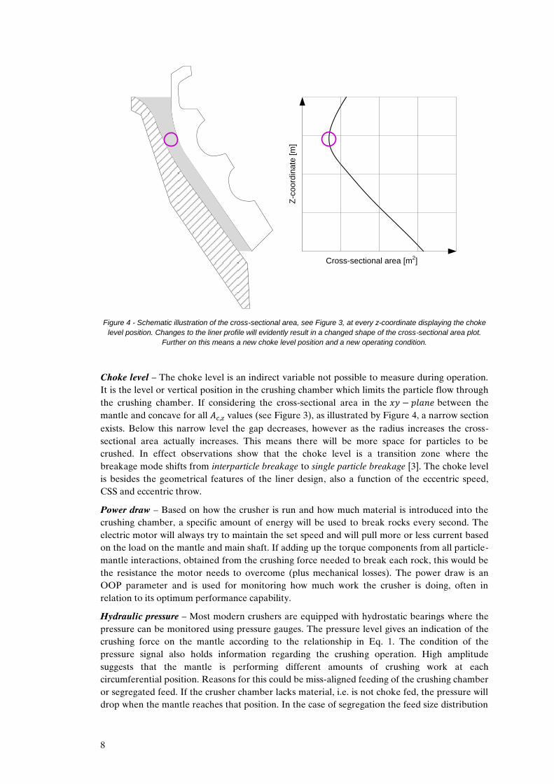
Figure 4 - Schematic illustration of the cross-sectional area, see Figure 3, at every z-coordinate displaying the choke

level position. Changes to the liner profile will evidently result in a changed shape of the cross-sectional area plot.

Further on this means a new choke level position and a new operating condition.

Choke level – The choke level is an indirect variable not possible to measure during operation. It is the level or vertical position in the crushing chamber which limits the particle flow through the crushing chamber. If considering the cross-sectional area in the 𝑥 𝑙 between the mantle and concave for all values (see Figure 3), as illustrated by Figure 4, a narrow section exists. Below this narrow level the gap decreases, however as the radius increases the cross-sectional area actually increases. This means there will be more space for particles to be crushed. In effect observations show that the choke level is a transition zone where the breakage mode shifts from interparticle breakage to single particle breakage [3]. The choke level is besides the geometrical features of the liner design, also a function of the eccentric speed, CSS and eccentric throw.

Power draw – Based on how the crusher is run and how much material is introduced into the crushing chamber, a specific amount of energy will be used to break rocks every second. The electric motor will always try to maintain the set speed and will pull more or less current based on the load on the mantle and main shaft. If adding up the torque components from all particle-mantle interactions, obtained from the crushing force needed to break each rock, this would be the resistance the motor needs to overcome (plus mechanical losses). The power draw is an OOP parameter and is used for monitoring how much work the crusher is doing, often in relation to its optimum performance capability.

Hydraulic pressure – Most modern crushers are equipped with hydrostatic bearings where the pressure can be monitored using pressure gauges. The pressure level gives an indication of the crushing force on the mantle according to the relationship in Eq. 1. The condition of the pressure signal also holds information regarding the crushing operation. High amplitude suggests that the mantle is performing different amounts of crushing work at each circumferential position. Reasons for this could be miss-aligned feeding of the crushing chamber or segregated feed. If the crusher chamber lacks material, i.e. is not choke fed, the pressure will drop when the mantle reaches that position. In the case of segregation the feed size distribution

Cross-sectional area [m2]

Z-c

oo

rdin

ate

[m

]

9

will be different at all circumference positions inevitably giving different bed confinement characteristics hence different force response.

2.1.2 Feeding conditions

The presentation of rock material to the crusher, i.e. feeding of the crusher, is one of the most crucial operational factors. Normally vibrating feeders or belt conveyors are used for feeding material to the crusher feeding box. In many cases this arrangement is not sufficient in order to achieve satisfying feeding conditions.

Figure 5 - DEM simulation of the feeding of a cone crusher. The picture clearly shows the segregation behaviour as

well as the proportionally higher amount of material in the right section of the crusher chute. (Unpublished work by

Quist)

As implied in the previous section many crushers are to some degree badly fed and experience two different issues; misaligned feeding and segregation. Misaligned feeding means that the material is not evenly distributed around the circumference hence there will be different amounts of rock material at all φ-positions. When operating under full choke fed condition the misaligned feeding is less of a problem. Segregation means that the particle size distribution will be different at φ-positions around the circumference. The reasons for these issues are coupled to how material is presented and distributed in the crusher rock box. When using a belt conveyor as a feeder the material can segregate very quickly on the belt. This segregation propagates into the crusher and is amplified when the rock stream hits the spider cap, see Figure 5. The spider cap acts as a splitting device causing coarse particles to continue to the back of the crusher and fine particles to bounce to the front. As the material has a horizontal velocity component in order to enter the crusher a large fraction of mass will end up in the back and a lower fraction of mass in the front. This effect is less when using vibrating feeders instead of conveyors as the horizontal velocity component is lower. For a more thorough investigation and description of this issue and ways to resolve it, the reader is advised to see Quist [7].

The operational effects of these issues are that the crusher effectively will perform as a different crushing machine at all φ-positions. As already stated this means that the hydraulic pressure will vary as the mantle makes one revolution. The result can be fatigue problems leading to main

10

shaft failure, cracks in the supporting structure, uneven liner wear, poor performance and control as well as many other problems due to that the machine is run in an unbalanced state.

2.1.3 Rock mass variation

For most aggregate quarries as well as mining sites the mineralogical content of the rock mass varies throughout the available area. This results in variation of the rock characteristics momentarily as well as on a long term basis. Meaning that the best operating parameters today may not be optimal next month, week or maybe even next hour [6]. When varying the rock competency the size distributions produced up-stream will slightly change giving new feeding material characteristics.

2.2 The Discrete Element Method

DEM is a numerical method for simulating discrete matter in a series of events called time-steps. By generating particles and controlling the interaction between them using contact models, the forces acting on all particles can be calculated. Newton’s second law of motion is then applied and the position of all particles can be calculated for the next time-step. When this is repeated it gives the capability of simulating how particles are flowing in particle-machine systems, see Figure 6. It is also possible to apply external force fields in order to simulate the influence of e.g. air drag or electrostatics. By importing CAD geometry and setting dynamic properties the environment which the rock particles is subjected to can be emulated in a very precise manner. This gives full control over most of the parameters and factors that are active and interesting during a crushing sequence. Also, due to the fact that all particle positions, velocities and forces are stored in every time-step, it is possible to observe particle trajectories and flow characteristics.

Figure 6 - Illustration of the DEM calculation loop used in EDEM

2.2.1 Approaches for modelling breakage

As the main purpose of this work is to break rocks in a simulation environment the choice of breakage model is important. Two different strategies dominate when it comes to modelling rock breakage in DEM – The population balance model (PBM) and the bonded particle model (BPM). The population balance model is based on the principle that when a particle is subjected to a load exceeding a specific strength criterion it will be replaced by a set of progeny particles of predetermined size. The strength criteria values and progeny size distribution are gathered from calibration experiments. This method is suitable for simulating comminution systems where impact breakage is the dominant breakage mode. The method has however been

11

used for modelling cone crushers as well [8]. The BPM method is based on the principle of bonding particles together forming an agglomerated cluster. Despite the fact that the PBM approach is more computationally effective and easy to calibrate the BPM approach is chosen for this work. The first reason is that the performance of a cone crusher is highly dependent on the particle flow dynamics within the crushing chamber. When using the PBM approach the particle dynamics are decoupled as the progeny particles are introduced at the same position as the broken mother particle. Hence the model cannot take into consideration particle movement as a result of a crushing sequence. This is not a problem in the BPM approach as the meta-particles are actually broken apart into smaller clusters. This leads up to the second reason which is that the PBM model is not based on simulating a crushing sequence but is basically only making use of the possibility to calculate forces on particles in DEM. The breakage itself is governed by an external breakage function. In conclusion the PBM approach basically uses the DEM model as an advanced selection function.

2.2.2 Previous work on DEM and crushing

A few publications exist on the topic of using DEM for rock crushers and cone crushers in particular. In the case of impact crushers Djordjevic and Shi [9] as well as Schubert [10] have simulated a horizontal impact crusher using the BPM approach. However in both cases relatively few particles have been used and the geometries are very simplified. A DEM model for simulating rock breakage in cone crushers has been presented by Lichter and Lim [8]. However, this model was based on a population balance model (PBM) coupled with a breakage function. This means that when a particle is subjected to a load greater then a threshold value it will be considered broken and the model replaces the mother particle with a set of progeny particles, sized according to the breakage function. This approach is very powerful in respect of computational efficiency but the actual breakage events are controlled by statistical functions, hence it is possible to tune the simulation towards performing according to experiments without knowing if the particle flow through the chamber is correct. Another aspect is the relationship between loading condition on a particle and particle breakage. Depending on a 1:1, 2:1, 2:2 or 3:1 point loading between two plates the rock will break differently. Generally, a rock particle subjected to a load will either be; undamaged, weakened, abraded, chipped, split or broken. In the PBM approach only the last effect is considered. Therefore current work is based around the more computational cumbersome Bonded Particle Model (BPM). This method has been previously utilized by the author for modelling a cone crusher [7, 11] as well as a primary gyratory crusher [12].

2.2.3 Hertz-Mindlin Contact model

The Hertz-Mindlin contact model, Figure 7 is used for accurately calculating forces for particles-particle and particle-geometry interactions in the simulation [13]. The normal force component is derived from Hertzian contact theory [14] and the tangential component from work done by Mindlin [15].

12

Figure 7 - Schematic illustration of the Hertz-Mindlin contact model used in EDEM.

Damping components are added to normal and tangential force components where damping coefficients are linked to the coefficient of restitution. The normal force is given by considering the normal overlap according to,

√

⁄ Eq. 2

The damping force is given by,

√ ⁄ √

�� Eq. 3

Where the equivalent Young’s modulus , equivalent radius , equivalent mass , damping coefficient and stiffness are given by,

Eq. 4

Eq. 5

(

)

Eq. 6

𝑙

√𝑙 Eq. 7

√ Eq. 8

, – Young’s modulus for spheres in contact

, – Poisson ratio for spheres in contact

, – Radius for spheres in contact

– Coefficient of restitution

The tangential force component is defined as the tangential stiffness times the tangential overlap. In addition the tangential damping force and tangential stiffness is given by,

𝐵

𝑠

𝑡 𝑜𝑟 𝑙

𝑡 𝑔 𝑡𝑖 𝑙 𝑥𝐵 ,𝑙𝑜𝑐 𝑙

𝐵 ,𝑙𝑜𝑐 𝑙

𝑧𝐵,𝑙𝑜𝑐 𝑙

,𝑙𝑜𝑐 𝑙

𝑥 ,𝑙𝑜𝑐 𝑙

𝑧 ,𝑙𝑜𝑐 𝑙

13

Eq. 9

√ ⁄ √

�� Eq. 10

√ Eq. 11

2.2.4 Contact model calibration

When using DEM for modelling breakage most of the focus is put on making sure that the contact model governing the fragmentation corresponds to a realistic behaviour. However it is very important to make sure that the contact model controlling flow behaviour is calibrated as well. If the friction parameters are not correct the particles will flow in an incorrect manner. When compressed the particles may e.g. slip and escape compression when in reality it would be nipped and broken.

No generally accepted method exists for calibrating contact models towards good flow behaviour. Hence a calibration device has been designed and built by CRPS [16]. A CAD model of the device can be seen in Figure 8. The device consists of an aluminium mainframe that holds a bottom section with a removable sheet metal floor and fixed sides. The top section holds a hopper with variable aperture and angle as well as a sliding plane with variable angle. The height of the top section can be adjusted. The different adjustment possibilities enable tests with different conditions. It is very important when calibrating a DEM contact model that it is independent of flow condition.

In Figure 9 an example of a calibration procedure can be observed. In the left picture the particle flow has been captured using a high speed camera. By iteratively varying parameters, simulating and comparing with the reference a decent set of values for the friction parameters can be found.

14

Figure 8 - DEM contact model calibration device developed by Quist at CRPS

Figure 9 - Snapshots from high speed video camera to the left and DEM simulation to the right.

15

2.2.5 The Bonded Particle Model

The BPM model was published by Potyondy and Cundall [17] for the purpose of simulating rock breakage. The approach has been applied and further developed by Cho [18]. The concept is based on bonding or gluing a packed distribution of spheres together forming a breakable body. The particles bonded together will here be called fraction particles and the cluster created is defined as a meta-particle. The fraction particles can either be of mono size or have a size distribution. By using a relatively wide size-distribution and preferentially a bi-modal distribution the packing density within the meta-particle increases. It is important to achieve as high packing density as possible due to the problematic issue with mass conservation as the clustered rock body will not be able to achieve full solid density. Also, when the bonded particle cluster breaks into smaller fragments the bulk density will somewhat change as area new particle size distribution is generated.

Figure 10 - Schematic representation of; (a) two particles overlapping when interacting giving a resultant force

according to the contact model seen in Figure 7. (b) two particles bonded together with a cylindrical beam leading to a

resultant force as well as normal and shear torques(modified from [17, 19]).

Figure 11 - Schematic force-displacement plot of the different modes of loading on a bond beam. The stiffness's and

critical stress levels are also shown. (Modified from [18])

The forces and torques acting on the theoretical beam can be seen in Figure 10. The schematic graph in Figure 11 illustrates the relationship between different loading modes (tension, shear, and compression), bond stiffness and strength criteria. Before bond-formation and after bond

𝑖

𝑖

𝑡��

𝑡��

𝑖

𝑏 2 𝑏

𝑖,𝑏 𝑏

𝑏𝑠

(a) (b)

𝑐𝑠

𝑐

Bond breaks

𝑏𝑠

𝑏

𝑠

Bond breaks

Compression

Tensio

n

Shear

1 1

16

breakage the particles interact according to the Hertz-Mindlin no slip contact model. The bonds are formed between particles in contact at a pre-set time 𝑡 . When the particles are bonded the forces and torques are adjusted incrementally according to the following equations:

Eq. 12

Eq. 13

Eq. 14

Eq. 15

Where,

𝑡

𝑡

𝑡

𝑡

Eq. 16

The normal and shear stresses are computed and checked if exceeding the pre-set critical stress values according to the equations below:

Eq. 17

Eq. 18

In this work the critical strength levels are set to a single value defining the rock strength. For future work it would be preferable to be able to randomize the critical bonding strength within a specified range or according to a suitable probability function.

2.2.6 Future DEM capabilities

DEM is a very computational intensive method. The continuous development of CPU speed enables larger particle systems to be modelled and by using several CPU processors in parallel the computational capacity is improving. However, since 5-10 years back Graphics Processing Units (GPU) have been adopted and used for computational tasks due to the high potential for parallelization. While a normal DEM simulation commonly utilizes 2-16 CPU cores a high-end GPU consists of 400-500 cores. If utilized effectively, this has the potential to dramatically increase the computational capacity by 10-100 times. But it is not as easy as just recompiling the source code and starting running on GPUs. The algorithm needs to be adopted to be run in parallel on all the GPU-cores, a task which has been proven as difficult, but not impossible. The developer community is vivid and the library of available functions is steadily increasing. A few DEM vendors have beta versions of GPU-based DEM codes and these will probably be available on the market in a few years.

17

2.3 Compressive breakage

It has been found by Schönert [20] that the most energy efficient way of reducing the size of rock is to use slow compressive crushing. Each particle can be loaded with the specific amount of energy needed to generate fracture resulting in progeny particles with a wanted size and specific surface.

2.3.1 Single Particle Breakage

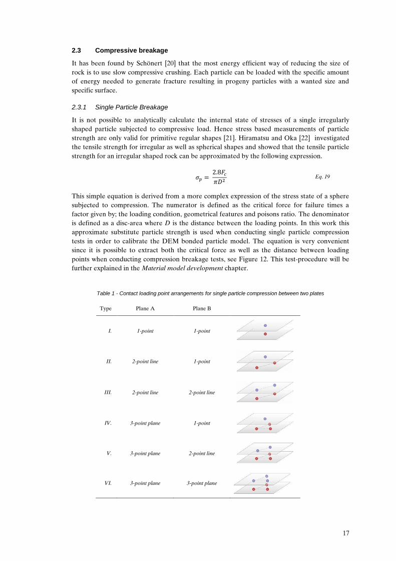
It is not possible to analytically calculate the internal state of stresses of a single irregularly shaped particle subjected to compressive load. Hence stress based measurements of particle strength are only valid for primitive regular shapes [21]. Hiramatsu and Oka [22] investigated the tensile strength for irregular as well as spherical shapes and showed that the tensile particle strength for an irregular shaped rock can be approximated by the following expression.

Eq. 19

This simple equation is derived from a more complex expression of the stress state of a sphere subjected to compression. The numerator is defined as the critical force for failure times a factor given by; the loading condition, geometrical features and poisons ratio. The denominator is defined as a disc-area where D is the distance between the loading points. In this work this approximate substitute particle strength is used when conducting single particle compression tests in order to calibrate the DEM bonded particle model. The equation is very convenient since it is possible to extract both the critical force as well as the distance between loading points when conducting compression breakage tests, see Figure 12. This test-procedure will be further explained in the Material model development chapter.

Table 1 - Contact loading point arrangements for single particle compression between two plates

Type Plane A Plane B

I. 1-point 1-point

II. 2-point line 1-point

III. 2-point line 2-point line

IV. 3-point plane 1-point

V. 3-point plane 2-point line

VI. 3-point plane 3-point plane

18

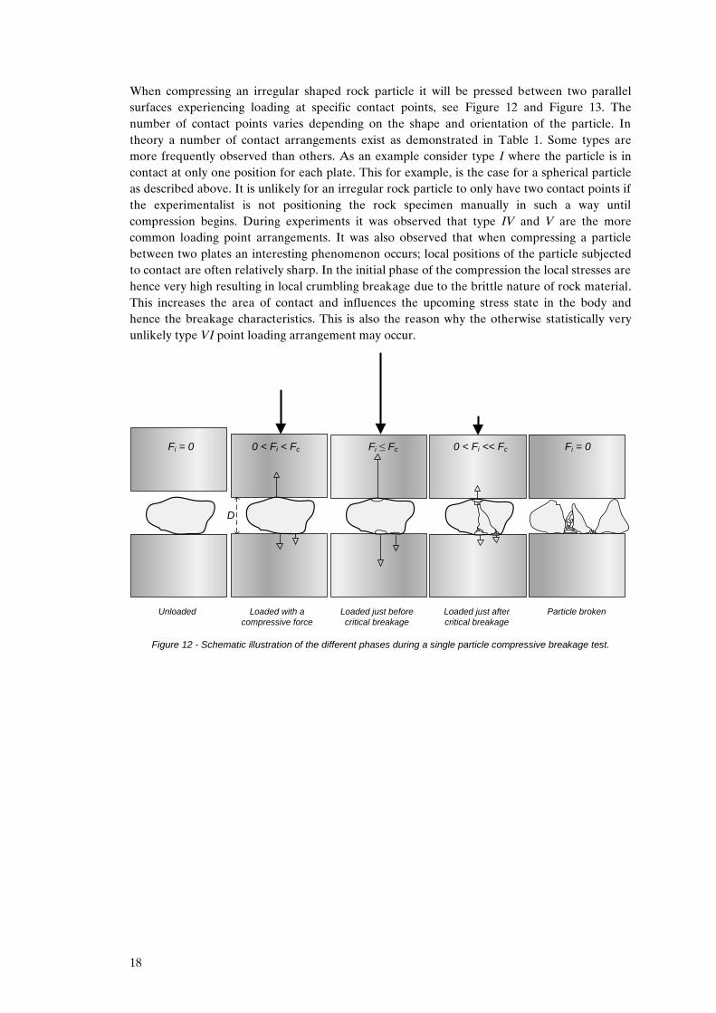
When compressing an irregular shaped rock particle it will be pressed between two parallel surfaces experiencing loading at specific contact points, see Figure 12 and Figure 13. The number of contact points varies depending on the shape and orientation of the particle. In theory a number of contact arrangements exist as demonstrated in Table 1. Some types are more frequently observed than others. As an example consider type I where the particle is in contact at only one position for each plate. This for example, is the case for a spherical particle as described above. It is unlikely for an irregular rock particle to only have two contact points if the experimentalist is not positioning the rock specimen manually in such a way until compression begins. During experiments it was observed that type IV and V are the more common loading point arrangements. It was also observed that when compressing a particle between two plates an interesting phenomenon occurs; local positions of the particle subjected to contact are often relatively sharp. In the initial phase of the compression the local stresses are hence very high resulting in local crumbling breakage due to the brittle nature of rock material. This increases the area of contact and influences the upcoming stress state in the body and hence the breakage characteristics. This is also the reason why the otherwise statistically very unlikely type VI point loading arrangement may occur.

Figure 12 - Schematic illustration of the different phases during a single particle compressive breakage test.

Unloaded Loaded with a

compressive force

Loaded just before

critical breakage

Fi = 0 0 < Fi < Fc Fi ≤ Fc 0 < Fi << Fc Fi = 0

Loaded just after

critical breakage

Particle broken

D

19

Figure 13 - Photo of an amphibolite particle from the feed sample subjected to compressive breakage

2.3.2 Inter Particle Breakage

Inter particle breakage can be defined as the breakage mode where a bed of particles is compressed and broken within a confined or unconfined space. During compression, forces transmigrate though the bed from particle to particle creating a force network. The packing structure is hence of interest when studying bed breakage. Several parameters influence the packing structure of a material bed;

Particle size distribution Particle shape Internal friction Wall friction Solid density

When a bed of particles is loaded the particles re-arrange slightly until a static condition is reached. The bed is then elastically compacted until particles start to fracture. Some research has been conducted in the field of interparticle breakage in order to better understand the complex mechanisms. Evertsson and Briggs [23] as well as Liu and Schönert [24, 25] have made important contributions. The discrete element method has been used as a tool for investigating interparticle breakage of mono-sized rocks and other agglomerates [26, 27]. Numerical FEM simulations of interparticle breakage in a confined space have been conducted by Liu [28]. The breakage of a bed of particles has been modelled in 2D FEM software in order to investigate the fragmentation behaviour when compressing the bed. In the beginning of the compression smaller particles are loaded in a quasi-uniaxial or quasi-triaxial compression mode. The smaller particles have fewer contact points then the larger particles hence the stress field generated has a higher local maximum stress resulting in crack propagation. Larger particles are surrounded by smaller fragments and hence experience a high number of contact points. As the displacement increases the larger particles will also experience high enough stresses to cause Hertzian crack propagation.

The interparticle breakage in a cone crusher happens either in a confined or an unconfined condition depending on the operation. An interesting question is how large the angular segment is where actual confined breakage takes place as the mantle moves eccentrically if the feeding condition changes.

20

3. METHOD

In this section all methods that have been applied or developed in the different phases of the project are presented with the aspiration that the reader should theoretically be enabled to reproduce the experiments and simulations. Focus will mainly be put on how methods and theories have been applied in contrast to the previous section where the theoretical background is introduced in a more general sense.

3.1 DEM as a CAE tool

The role for CAE tools at R&D departments in all industries is growing steadily. With new capabilities to simulate and evaluate design decisions during concepts or detail development, time and resources previously spent on expensive prototypes and field testing are better spent. The DEM method is a fairly new tool which is in its cradle when it comes to systematic usage by large R&D departments. Hence, few methodologies or frameworks exist for how or when to use DEM. DEM is one of many computational engineering techniques so the methodology emerged in the field of e.g. FEM could be interesting to review. As this method has been around for a much longer time a lot of research has been conducted on the management around FEM analysis.

During development and design of machines or processes which interact with granular material, it is commonly difficult to predict the behaviour and performance of the system. The types of situations where analysis and simulation are needed can roughly be categorized as follows;

Evaluation Problem solving Optimization Fundamental understanding

These four can be of interest both for new products as well as for existing products and implementations. It has been found in this work that in order to be effective and fully leverage the power of DEM it is crucial to adopt a statistical approach. When it comes to optimization and fundamental understanding where a high number of parameters need to be studied, it is recommended to use the design of experiment approach. As computational resources are usually scarce , fractional factorial analysis [29] is a good way of reducing the simulations needed in order to draw conclusions. In the case of e.g. concept evaluation or problem solving sometimes one single or very few simulations are needed in order to give enough information to make decisions. A framework for how to utilize DEM as a concept evaluation tool for design and problem solving of bulk materials handling applications, has been presented by Quist [7]. The work shows that the resolution or quality of the DEM model can be used actively for different purposes. When the objective is to do a quick concept screening a very simple model can be setup in order to give some information regarding basic flow trajectories and so on. Such quick simulations can be setup and simulated within one hour. By working in an iterative manner with the concepts and raising the resolution and quality of the DEM simulations accordingly the probability of succeeding with the development efforts is greatly enhanced.

3.2 Bonded Particle Model Rock Population

A rock material consists of a number of different minerals and crystalline structures with different mechanical properties. When considering the properties of a rock type the proportion of the various minerals is subject to analysis commonly by doing a petrographic analysis. The petrographic composition of the rock material in Kållered can be seen in Table 2. An example of the microstructure of granite rock can be seen in Figure 14. As can be seen it is constituted by

21

a number of different minerals. The mechanical property of the rock mass depends on the properties of each constituent, proportion, the grain architecture and size as well as weathering effects, cracks and defects.

Figure 14 - Illustration of the heterogeneous microstructure of a typical granite rock

Table 2 - Petrographic composition of the rock material in Kållered

Fraction (mm) Quantity Proportion (%) Meas. Uncert. (±%) Mineral type

2-4 171 17 2.3 Quartz

457 46 3.1 Feldspar

117 12 2.0 Mica (Biotite)

187 19 2.4 Amphibolite

67 7 1.5 Pot. alkali-reactive material

1 0.1 0.2 Ore-minerals incl. sulphides

3.2.1 Generating a bi-modal particle packing cluster

Different types of size distributions give varying packing performance as well as number of contact points as illustrated in Figure 15. Particles can be arranged in a number of different bravais lattice systems; [30]

Simple cubic (SC) Face-centred cubic (FCC) Body centred cubic (BCC) Hexagonal closed packing (HCP)

These packing structures mainly apply to crystalline structures made up of mono-sized or double mono size particle structures. The arrangement of the particles or atoms, together with the nature of bonding forces characterizes many of the mechanical properties of a material. When building a synthetic rock in the DEM environment the ambition is to capture as many of the features of real rock material as possible. If there was no computational constraint, one would try to model every atom, molecule or mineral grain. However, currently there is a trade-off between the number of meta-particles we want to model and how many particles we put in each meta-particle. Most of the work and simulations done on rock breakage using bonded particle models focus on the breakage of a single particle in e.g. a uniaxial strength test. In this case it is possible to capture a fairly accurate breakage mechanism using all the available particles for one rock specimen. This approach is of course irrelevant when trying to create a rock population for crushing.

22

Figure 15 - Schematic illustration of three different packing structures given by different types of size distributions.

When applying a bonding model to these clusters the contact lines seen in the illustration would become boding

beams. Hence the strength characteristics of a particle built up by a packed set of spheres strongly depends on the

packing structure and size distribution.

In this work it was found that the most suitable approach to model the breakage of rock particles is to use a bi-modal distribution with relatively large particles in the high end with smaller particles acting as cement in between, as demonstrated in the illustration to the right in Figure 15. An example of the contact network generated from a particle bed with bimodal distribution can be seen in Figure 16. When activating the bonding function in the simulation these contacts are converted to bonds.

Figure 16 - Contact network generated by a particle bed with bimodal distribution. The colours represent the length of

the contact vector and show that the body is highly heterogeneous.

The following procedure has been developed for creating a particle packing cluster with a bimodal distribution suitable for a BPM in EDEM;

i. Create two cylinders with appropriate diameter to fit the wanted end particle size. One should be the container and the other the particle factory. The container cylinder should be placed around origo so that when a 3D particle geometry later is imported it will be fully surrounded by particles.

ii. Define a material with low static friction and a higher stiffness then used later. iii. Define a spherical particle named Fraction with a nominal particle size between the coarse and fine modals

of the distribution. The contact radius should be set slightly higher than the physical radius. iv. Define a particle factory for the coarse end of the distribution with a capped normal distribution with e.g.

µ=2 and capped in the range 1<µ<3. Set the time stamp to tstart=0s. v. Define a particle factory for the fine end of the distribution with a capped normal distribution with e.g.

µ=0.8 and capped in the range 0.6<µ<1. Set the time stamp to tstart=tstep.

ii: Gaussian distributioni: Mono distribution iii: Bimodal distribution

-

-

--

-

-

- -

- -

-

--

-

-

-

-

-

-

--

--

-- -

-

-

---

--

--

-

-

--

-

- -

-

-

--

-

--

-

--

- -

-

-

-

--

-

-

-

---

-

-

-

- -

-

---

-

--

-

-

-

--

-

-

-

--

--

- -

-

-

-

-

-

- -

--

-

-

23

vi. Let the particles settle forming a loosely packed bed see Figure 17. Due to a higher stiffness the overlaps will be reduced compared to if using the actual stiffness later. By doing so the risk of a preloaded bed is lowered.

vii. Define a selection space by importing rock shaped geometry, see Figure 17. viii. Export the particle positions (X,Y,Z) and radius for all particles within the selection space

ix. Reorganize the exported data in the following way;

271

0.0165135 0.0097095 -0.00677124 2.418

0.00664328 -0.0377409 0.00264027 2.123

-0.0288484 0.00226568 -0.00600659 1.594

…

The first position is how many particles the cluster contains. The first, second and third rows are X, Y, Z coordinates and the fourth is the scaling factor.

Figure 17 - The picture to the left show a bimodal particle bed created in step (vi) above. The middle picture shows

the 3D rock selection space imported in step (vii). The picture to the right shows the selection of particles within the

selection space as done in step (viii)

3.2.2 Calibration of the bonded particle model

As mentioned in previous chapters rock breakage experiments are often conducted on primitive shapes such as a cylinder in the uniaxial strength test due to the possibility to calculate the internal stress state. In this work single particle breakage tests have been conducted on a set of rock particles from the test material sample. The critical force for failure and the rock size was recorded. The particle strength given by Eq. 19 was applied in order to find a strength distribution. The calibration work performed in this work will be presented in detail in the Material Model Development chapter.

3.2.3 Introducing meta-particles by particle replacement

In EDEM particles are generated to the simulation environment by using particle factories. Usually geometry such as a box, cylinder or a plane is defined as a particle factory and the user can define what particles should be created at what rate. This approach is practical if the purpose of the simulation is to e.g. continuously generate material to a conveyor or create 100’000 particles at once in a mill. However this way of introducing particles is not sufficient when working with multiple dynamic BPM models.

It is possible to define custom factories in EDEM. In this work a special approach is used for creating the meta-particles. First a set of dummy particles is created for each meta-particle size class using standard box geometry as factory. These particles are single spheres and have to be larger than the meta-particle cluster. When a set of dummy particles has been generated each

24

dummy particle is used as a custom factory. A custom factory, called Particle Replacement Factory creates fraction particles according to the coordinates and sizes defined in the meta-particle cluster coordinate file. Fraction particles are placed inside the dummy particles according to the local coordinate system of the dummy particle. This is why it has to be larger than the cluster. When the fraction particles are in place, the dummy particle is removed. An example of this procedure can be seen in Figure 18.

Figure 18 - Snapshot from EDEM showing a stage in the particle replacement procedure. In the picture a set of meta-

particles has been created and a new set of large dummy particles can be seen for the next replacement action.

3.3 Industrial scale crusher experiments

Industrial scale experiments have been conducted at a quarry owned by Jehander Sand & Grus AB located in Kållered, south of Göteborg. The site has several cone crushers in process for both secondary and tertiary operations. The secondary crusher, a Svedala H6000 cone crusher, was chosen for the experiments. The ambition with the tests has been to fully capture all possible data concerning both the feed material, machine operation and product material. When conducting tests on a secondary crusher operation normally it is problematic to sample the feed material and do sieve analysis due to the large sized rocks. Rock particles are up to 250 mm in size with a considerable mass for each rock. This has consequences on the statistical significance as a minimum number of particles should be sampled for each size class. If following the recommendations in European standards several tons of feed materials need to be sampled. This is not feasible hence as much material as possible has been sampled and sieved. While digging off material from the belt is a relatively simple task, sizing the rocks bigger then 45mm is cumbersome. It is very rare with mechanical sieves with aperture size larger than 90mm. The lab on site has a vibrating sieve with largest aperture of 45 mm. In order to size particles larger than this a set of square sizing-frames was designed and manufactured, see Figure 19.

25

Figure 19 - Feed sizing with sizing-frames designed in the project

In Table 3 a test plan for the full scale experiments in Kållered can be seen. Five different runs have been performed at CSS ranging from 34 to 50 mm. Belt cuts are extracted from the product belt for each run and the feed sampled for the first, third and fifth run.

Table 3 – Industrial scale experiment test plan

SVULLO EXPERIMENTS

Time frame with feed cut Run CSS Samples D. Time [min] Tot. Time [min]

Activity Quist Activity Åberg Time Up-Time D. Time RUN1-34 34 F+P 12,5 22,5

1 Set CSS 0,5 0,5 RUN2-38 38 P 10 15

2 Lead CSS calibration 5 5 RUN3-42 42 F+P 12,5 22,5

4 Start DAQ Measurement 1 1 RUN4-46 46 P 10 15

5 Run Crusher 3 3 RUN5-50 50 F+P 12,5 22,5

6 Make time note 0,5 0,5 57,5 97,5

7 Stop DAQ Measurment Stop Belts 1 1

8 Lock OFF belts 0,5 0,5 Samples Expected weight Item Quantity

9 Do belt cut (Feed) Do belt cut (Product) 10 10 S1-34-P 40 Sampling Equipment

10 Lock ON 0,5 0,5 S2-38-P 40 Buckets (20l) 30

11 Start belts 0,5 0,5 S3-43-P 40 Sack 10

22,5 10 12,5 S4-46-P 40 Brush 1

S5-50-P 40 Shovel 1

S1-34-F 40 Spade 2

Time frame without feed cut S3-43-F 40 Tape 2

Activity Quist Activity Åberg Time Up-Time D. Time S5-50-F 40 Tape measure 2

1 Set CSS 0,5 0,5 320 kg Scale 1

4 Start DAQ Measurement 1 1 Sampling Processing Equipment

5 Run Crusher 3 3 Oven 1

6 Make time note 0,5 0,5 Sieve Shaker 1

7 Stop DAQ Measurment Stop Belts 1 1 Corse Sieves 6

8 Lock OFF belts 0,5 0,5 Shape Index meter 1

9 Do belt cut (Product) Do belt cut (Product) 7,5 7,5 Scale 1

10 Lock ON 0,5 0,5

11 Start belts 0,5 0,5

15 5 10

26

A test-sequence was created in order to manage the experiment. This was done due to several reasons such as personal safety; minimize the risk of data and sample loss; quality of samples and time management. Before the first test the process was operated until it reached a steady condition. Then a dry run was performed in order to test each action. The tests followed the following sequence of actions;

1. Set CSS 2. Start feeding 3. Run until choked condition 4. Start data logging and run for 3 minutes 5. Stop incoming feed 6. Stop data logging 7. Stop conveyors 8. Perform lock-out on conveyors 9. Do belt cut 10. Rendezvous at station and lock on

All product samples were handled in plastic buckets with handles and lids that prevent moisture from escaping, see Figure 20. Each bucket was weighed after the experiments as a control measure and as a reference for moisture content. The feed samples were handled in tough reinforced polymer bags due to the large sized rock particles.

Figure 20 - All the material sampled during the experiments placed in the lab before sample processing.

The product samples have been processed in accordance with European standard EN933-1. First each sample was sieved using the large vibrating sieve with an 8mm bottom deck and 63 mm top deck. Each sample was hence split at 8 mm. The large size fraction was simply weighed due to the low amount of moisture in the large size fraction. The minus 8 mm material was split down to 2+2 kg and dried for 2 hours. Each 2 kg sample was then sieved in a conventional cylindrical vibrating screen in order to retrieve the total size distribution from 63 µm to 63 mm. One of the product samples after the coarse sieving can be seen in Figure 21.

27

Figure 21 - Picture showing each size class during coarse sieve processing as well as the minus 8 mm material.

In Figure 22 one of the feed samples can be seen. All rocks larger than 45 mm have been individually tested in the sieve-frames and put in the corresponding box. The picture also gives an indication of the size distribution of the feed.

Figure 22 - The picture shows each size class from the manual sieve analysis of one of the feed samples.

3.4 Crusher geometry modelling

One of the most difficult obstacles to overcome when trying to simulate and replicate the behaviour of a real crusher is to create a good geometrical model. The easy method is to use nominal CAD geometry. However these geometries do not take wear or liner design changes into consideration. Even if it is known what type of mantle and concave should be installed it is very difficult to know for sure when looking at the liners in operation. Also it may be very difficult to get hold of the CAD geometry for each specific liner profile.

In this project this was solved by 3D-scanning both the mantle and the concave two weeks after the experiments had been performed. The scanner used is a FARO FOCUS3D laser scanner provided and owned by Roctim AB. The ambition was to perform the scanning inside the plant workshop in a controlled environment. However due to operational issues on site, the liners were never moved. Hence the scanning was performed outdoors without possibility to arrange the liners in a suitable way, see Figure 23.

28

Figure 23 - Left: test scan of a mantle in the mechanical workshop. Right: position of the concave and top frame when

scanning. The concave was positioned in a slope hence the scanning procedure was problematic.

In Figure 24 a planar view of the 3D scan of the concave is shown. The scanner was placed inside the mantle at two positions in order to capture the full concave geometry. Due to the position on the ground it was difficult to get a high quality scan. If the concave would have been placed inside the workshop on a support structure it would have been in level and possible to clean before scanning.

Figure 24 - Snapshot from the 3D-scanning post-processing software showing the unwrapped model of the concave

and spiderarms with a color map applied to it.

Ideally when scanning a mantle it should be positioned as seen in Figure 23. However the mantle of interest had to be scanned on its position after maintenance hence only a section was captured as shown in Figure 25.

29

Figure 25 - Snapshot of the mantle from the 3D-scan post-processing software.

Since it was difficult to capture the full mantle and concave geometries an alternative approach was used for creating a representative liner profile. From both the mantle and concave scan data a set of section samples was extracted and imported to CatiaV5. By drawing spline curves on these sections and finding a best mean a representative profile has been found. The final mantle and concave surfaces were generated by revolving the spline profile around the centre axis.

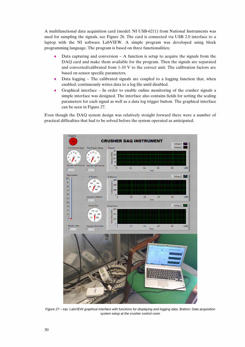
3.5 Crusher data acquisition

A data acquisition system has been developed for sampling data at high frequency from the available crusher sensors. Pressure, power draw, shaft position and temperature signals have be sampled by using opto-isolators splitting the signal from the installed crusher control system. In this work only the pressure and power draw signals have been analysed. The motive behind using a secondary data acquisition system instead of extracting data from the installed control system is based on the suspicion of signal aliasing. The installed system samples data at 10 Hz which is a too slow frequency to capture the true nature of the signals as will be shown in the next chapter.

Figure 26 - NI USB-6211 data acquisition card

30

A multifunctional data acquisition card (model: NI USB-6211) from National Instruments was used for sampling the signals, see Figure 26. The card is connected via USB 2.0 interface to a laptop with the NI software LabVIEW. A simple program was developed using block programming language. The program is based on three functionalities;

Data capturing and conversion – A function is setup to acquire the signals from the DAQ card and make them available for the program. Then the signals are separated and converted/calibrated from 1-10 V to the correct unit. The calibration factors are based on sensor specific parameters.

Data logging – The calibrated signals are coupled to a logging function that, when enabled, continuously writes data to a log file until disabled.

Graphical interface – In order to enable online monitoring of the crusher signals a simple interface was designed. The interface also contains fields for setting the scaling parameters for each signal as well as a data log trigger button. The graphical interface can be seen in Figure 27.

Even though the DAQ system design was relatively straight forward there were a number of practical difficulties that had to be solved before the system operated as anticipated.

Figure 27 – top: LabVIEW graphical interface with functions for displaying and logging data. Bottom: Data acquisition

system setup at the crusher control room

31

4. CRUSHER EXPERIMENT

The aim of the following section is to present the results from the industrial scale experiments performed in the project. The data shown will be presented and commented on independently from the simulation results.

4.1 Size reduction

The product particle size distribution for the five different tests as well as the feed particle size distributions can be seen in Figure 28. As anticipated the product gets finer when reducing the gap setting apart from the CSS42 sample that deviates from expectations. The reason for this deviation is unknown but could be either related to a mistake in the sampling, sampling processing or the post processing. It could also be due to stochastic variation in the feed. As can be seen the feed samples differ relatively much in the CSS42 feed sample which could also be the reason for the deviation. As previously mentioned a very large feed sample is preferred in order to achieve statistical significance, hence the three different samples have been combined as a representation of the total feed sample.

Figure 28 - Feed and product particle size distributions for the five different CSS settings.

The throughput capacity for the five different tests can be seen in Figure 29. The data collected during a previous survey on the same process is also shown as a reference. Both data sets suggest a non-linear relationship between close side setting and capacity. An interesting feature of the curve shape is the mid peak at 42 mm for the current tests and 44 mm for the old survey. The 2 mm difference may be due to difference in feed material or a gap calibration deviation. A possible explanation to the raising trend for higher CSS is that the cross-sectional area at the choke level gets slightly larger when increasing the gap setting.

0,0%

10,0%

20,0%

30,0%

40,0%

50,0%

60,0%

70,0%

80,0%

90,0%

100,0%

0,1 1 10 100

Cum

ula

tive P

assin

g [%

]

Aperture Size [mm]

CSS-34-P

CSS-38-P

CSS-42-P

CSS-46-P

CSS-50-P

FEED TOT

CSS-34-Fd

CSS-42-Fd

CSS-50-Fd

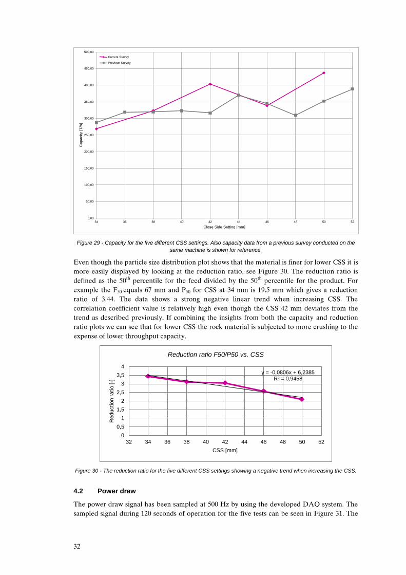
32

Figure 29 - Capacity for the five different CSS settings. Also capacity data from a previous survey conducted on the

same machine is shown for reference.

Even though the particle size distribution plot shows that the material is finer for lower CSS it is more easily displayed by looking at the reduction ratio, see Figure 30. The reduction ratio is defined as the 50th percentile for the feed divided by the 50th percentile for the product. For example the F50 equals 67 mm and P50 for CSS at 34 mm is 19.5 mm which gives a reduction ratio of 3.44. The data shows a strong negative linear trend when increasing CSS. The correlation coefficient value is relatively high even though the CSS 42 mm deviates from the trend as described previously. If combining the insights from both the capacity and reduction ratio plots we can see that for lower CSS the rock material is subjected to more crushing to the expense of lower throughput capacity.

Figure 30 - The reduction ratio for the five different CSS settings showing a negative trend when increasing the CSS.

4.2 Power draw

The power draw signal has been sampled at 500 Hz by using the developed DAQ system. The sampled signal during 120 seconds of operation for the five tests can be seen in Figure 31. The

0,00

50,00

100,00

150,00

200,00

250,00

300,00

350,00

400,00

450,00

500,00

34 36 38 40 42 44 46 48 50 52

Capacity [

T/h

]

Close Side Setting [mm]

Current Survey

Previous Survey

y = -0,0806x + 6,2385R² = 0,9458

0

0,5

1

1,5

2

2,5

3

3,5

4

32 34 36 38 40 42 44 46 48 50 52

Reductio

n r

atio

[-]

CSS [mm]

Reduction ratio F50/P50 vs. CSS

33

signal amplitude is very high for all tests which normally indicate poor operation. The initial ambition was to sample the power draw signal from the plant control system, however this data was lost. When the test was conducted the power draw signal displayed by the plant control system did not show this large amplitude. It is strongly suspected that the sampling frequency of the control system is too low and that signal filtering is applied in such a way that the peaks are effectively removed.

Figure 31 - Power signals for five different CSS over two minutes of operation. Even though the amplitude is very high

the linear trend lines show a distinct difference in mean power draw.

As the plot in Figure 31 is very compact it is difficult to see what is actually going on. However the ambition is to show the clear difference in the average power draw when applying a linear regression line on each signal. Due to the large number of data points it is impossible to see what the signal looks like in detail. In Figure 32 the power draw signal for one second of operation is shown. Here it is clearly seen how the signal fluctuates at a specific frequency. The frequencies of the fluctuations are approximately 5 Hz which is the same as the mantle eccentric speed. This means that the variation is somehow related to the movement of the mantle. Recall from the theory chapter that the feeding of material is a vital aspect of a crusher operation. The probable cause of the fluctuations observed is hence miss-aligned feed and segregation. At the

34

peak angular position there is probably both a larger amount of material as well as a finer feed size distribution that requires more energy to be broken.

Figure 32 - Pressure signal measured during one second showing the highly fluctuating signal for all CSS settings.

The specific time span chosen for each test is randomly picked.

When operating any type of process it is of the essence to run it under statistical process control [29]. This generally means that variation from both stochastic as well as systematic sources should be limited. When the variation is suppressed the challenge is to keep the process stable and hence predictable. If the process is stable and predictable then it is possible to control it. The standard deviation of the power draw signal can be seen in Figure 33. The lowest variation can be seen for CSS 38mm.

Figure 33 - The standard deviation of the pressure signal is shown for the five CSS settings.

As previously mentioned and also seen in Figure 31 the signal has distinct average values. In Figure 34 the average power draw can be seen. The linear trend is very strong with a correlation coefficient of 0.9837. The data indicates that the crusher is working harder i.e. putting more energy into the rock bed per unit time, at lower CSS values. This also aligns with the previous

0

10

20

30

40

50

60

70

80

90

100

110

120

130

140

150

160

170

180

190

200

210

0 0,2 0,4 0,6 0,8 1

Pow

er

dra

w [

kW

]

Time [s]

Power draw during 1 second for 5 CSS

Power_CSS34

Power_CSS38

Power_CSS42

Power_CSS46

Power_CSS50

0

5

10

15

20

25

30

35

40

32 34 36 38 40 42 44 46 48 50 52

Pow

er

dra

w

Sta

. D

ev.

[kW

]

CSS [mm]

Power draw Std vs. CSS

35

results regarding higher reduction ratio at lower CSS as the electrical energy in the motor, via kinetic energy, is transformed to surface energy when the rocks break.

Figure 34 - The average power draw measured for the five CSS settings displaying a negative trend when increasing

the close side setting

4.3 Hydrostatic pressure

The pressure signals sampled at 500 Hz for 120 seconds are plotted in Figure 36. The same argument as in the case with the power draw signals can be made for the pressure signal. The signal has very high amplitude and appears to be noisy. However as previously described the amplitude is not a result of noise but due to cyclic behaviour in the crusher and super positioned discrete crushing events. A detailed view of two of the signals for one second of operation can be seen in Figure 35. The data reveals that the frequency of the variation matches the eccentric speed of the crusher. Hence this provides yet further evidence that the crusher is not fed in a satisfactory manner or there may be uneven wear on the concave.

Figure 35 - In order to get a closer look at the measured pressure signal one second of operation is displayed in the

plot for two of the CSS settings. The time span between each peak corresponds to the eccentric speed of the mantle.

y = -1,5462x + 181,82 R² = 0,9837

0

20

40

60

80

100

120

140

32 34 36 38 40 42 44 46 48 50 52

Avera

ge P

ow

er

Dra

w [

kW

]

CSS [mm]

Average Power draw vs. CSS

0

0,5

1

1,5

2

2,5

3

3,5

0 0,1 0,2 0,3 0,4 0,5 0,6 0,7 0,8 0,9 1

Pre

ssure

[M

Pa]

Time [s]

Pressure vs. time for two CSS

Pressure_34 Pressure_50

36

Figure 36 - Pressure signals for five different CSS over two minutes of operation. Even though the amplitude is very

high the linear trend lines show a distinct difference in mean pressure.

The standard deviation of the pressure signal can be seen in Figure 37. It is a bit difficult to draw conclusions regarding the shape of the curve. However assuming it is representative, it shows that the variation is slightly higher when pushing the crusher at lower CSS values. This may indicate that the small gap setting is more sensitive to segregation resulting in a larger variation. Hence if the ambition is to run a crusher at small setting in order to have a high reduction ratio, the feeding conditions are very important to consider in order to run the operation under statistical process control.

37

Figure 37 - The standard deviation of the measured pressure signal for the five CSS settings.

As in the case of the power draw the pressure shows a strong decreasing linear trend for increasing CSS, see Figure 38. The correlation coefficient is remarkably high at 0.9956 which indicates a successful experiment. An interesting detail is that there is no deviation from the trend for CSS 42 mm as in the case of the product size distribution and the reduction ratio.

Figure 38 - The average pressure for the five CSS settings showing a negative trend for increasing CSS. The very

strong linear correlation should be noted.

0

0,2

0,4

0,6

0,8

1

32 34 36 38 40 42 44 46 48 50 52

Pre

ssure

Std

. [M

Pa]

CSS [mm]

Pressure Std vs. CSS

y = -0,029x + 2,9453 R² = 0,9956

0

0,4

0,8

1,2

1,6

2

2,4

32 34 36 38 40 42 44 46 48 50 52

Avera

ge P

ressure

[M

Pa]

CSS [mm]

Average pressure vs. CSS

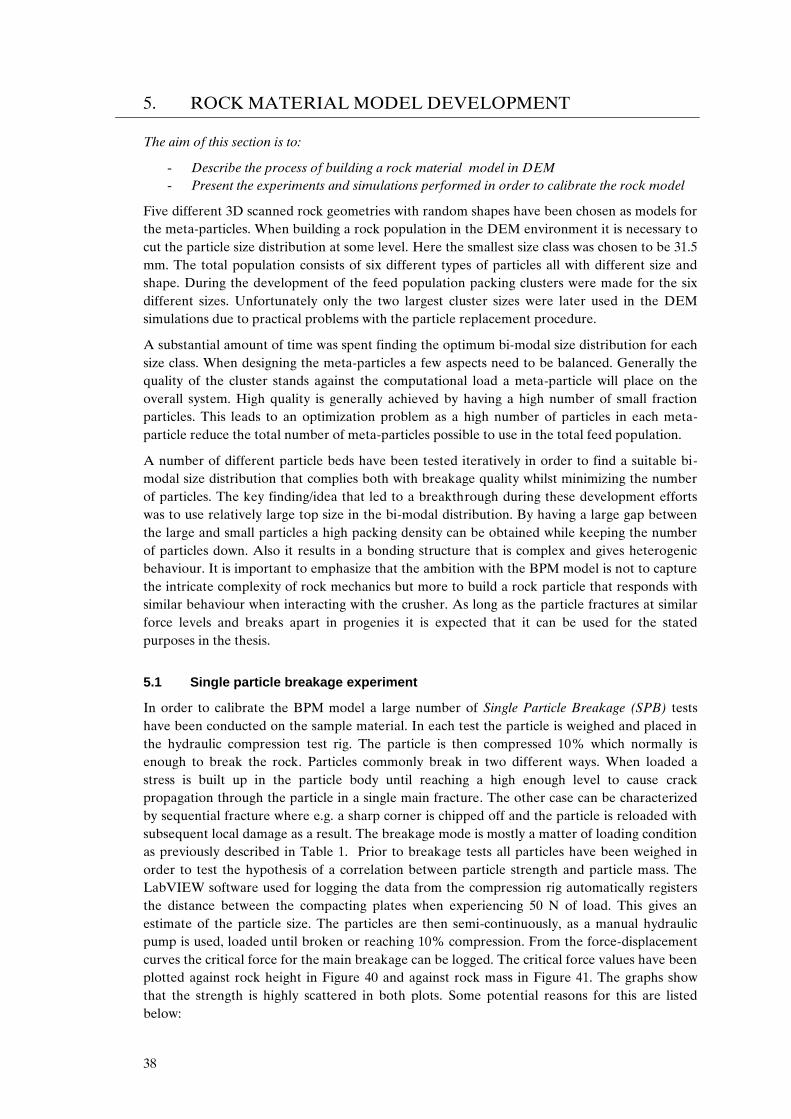
38

5. ROCK MATERIAL MODEL DEVELOPMENT

The aim of this section is to:

- Describe the process of building a rock material model in DEM - Present the experiments and simulations performed in order to calibrate the rock model

Five different 3D scanned rock geometries with random shapes have been chosen as models for the meta-particles. When building a rock population in the DEM environment it is necessary to cut the particle size distribution at some level. Here the smallest size class was chosen to be 31.5 mm. The total population consists of six different types of particles all with different size and shape. During the development of the feed population packing clusters were made for the six different sizes. Unfortunately only the two largest cluster sizes were later used in the DEM simulations due to practical problems with the particle replacement procedure.

A substantial amount of time was spent finding the optimum bi-modal size distribution for each size class. When designing the meta-particles a few aspects need to be balanced. Generally the quality of the cluster stands against the computational load a meta-particle will place on the overall system. High quality is generally achieved by having a high number of small fraction particles. This leads to an optimization problem as a high number of particles in each meta-particle reduce the total number of meta-particles possible to use in the total feed population.

A number of different particle beds have been tested iteratively in order to find a suitable bi-modal size distribution that complies both with breakage quality whilst minimizing the number of particles. The key finding/idea that led to a breakthrough during these development efforts was to use relatively large top size in the bi-modal distribution. By having a large gap between the large and small particles a high packing density can be obtained while keeping the number of particles down. Also it results in a bonding structure that is complex and gives heterogenic behaviour. It is important to emphasize that the ambition with the BPM model is not to capture the intricate complexity of rock mechanics but more to build a rock particle that responds with similar behaviour when interacting with the crusher. As long as the particle fractures at similar force levels and breaks apart in progenies it is expected that it can be used for the stated purposes in the thesis.

5.1 Single particle breakage experiment

In order to calibrate the BPM model a large number of Single Particle Breakage (SPB) tests have been conducted on the sample material. In each test the particle is weighed and placed in the hydraulic compression test rig. The particle is then compressed 10% which normally is enough to break the rock. Particles commonly break in two different ways. When loaded a stress is built up in the particle body until reaching a high enough level to cause crack propagation through the particle in a single main fracture. The other case can be characterized by sequential fracture where e.g. a sharp corner is chipped off and the particle is reloaded with subsequent local damage as a result. The breakage mode is mostly a matter of loading condition as previously described in Table 1. Prior to breakage tests all particles have been weighed in order to test the hypothesis of a correlation between particle strength and particle mass. The LabVIEW software used for logging the data from the compression rig automatically registers the distance between the compacting plates when experiencing 50 N of load. This gives an estimate of the particle size. The particles are then semi-continuously, as a manual hydraulic pump is used, loaded until broken or reaching 10% compression. From the force-displacement curves the critical force for the main breakage can be logged. The critical force values have been plotted against rock height in Figure 40 and against rock mass in Figure 41. The graphs show that the strength is highly scattered in both plots. Some potential reasons for this are listed below:

39

Stochastic orientation of particles Anisotropic structure and strength Particle shape difference and hence variation in loading condition which means totally

different stress fields within the rock body. Stochastic variation in the rock strength Variation in the compression movement due to manual hydraulic pump Variation due to robustness problems with the compression rig frame

Figure 39 shows the force displacement curves for 7 of the 116 performed SPB tests. As can be seen there is a staircase pattern due to the use of a manual hydraulic pump. Ideally these tests should be performed using a compressive rig with a motorized hydraulic pump where the rate can be controlled. As can be seen in the plot the force is built up until the particle breaks. The peak force at which breakage occurs is defined as the critical force.

Figure 39 - The figure shows the force-displacement plot for 7 of the 116 performed SPB tests. The staircase pattern

seen is related to the manual hydraulic pumping motion.

Figure 40 - Scatter plot of critical breakage force vs. rock height. The height is defined as the distance between the

plates when the rock is loaded by 50 N.

0

2000

4000

6000

8000

10000

12000

0% 1% 2% 3% 4% 5% 6% 7% 8% 9% 10%

Forc

e [N

]

Compression ratio [%]

SPB experiments - Force vs. Displacement

S1

S2

S3

S4

S5

S6

S7

R² = 0,3154

y = -7,6805x2 + 1119,8x - 13076

R² = 0,5278

y = 18,817x2 - 339,69x + 6793,1R² = 0,5609

0

10000

20000

30000

40000

50000

60000

70000

10 15 20 25 30 35 40 45 50 55 60

Fc [N

]

Rock height [mm]

Peak Force - Rock Height

Granite

Amphibolite

Linear (Granite)

Poly. (Granite)

Linear (Amphibolite)

Poly. (Amphibolite)

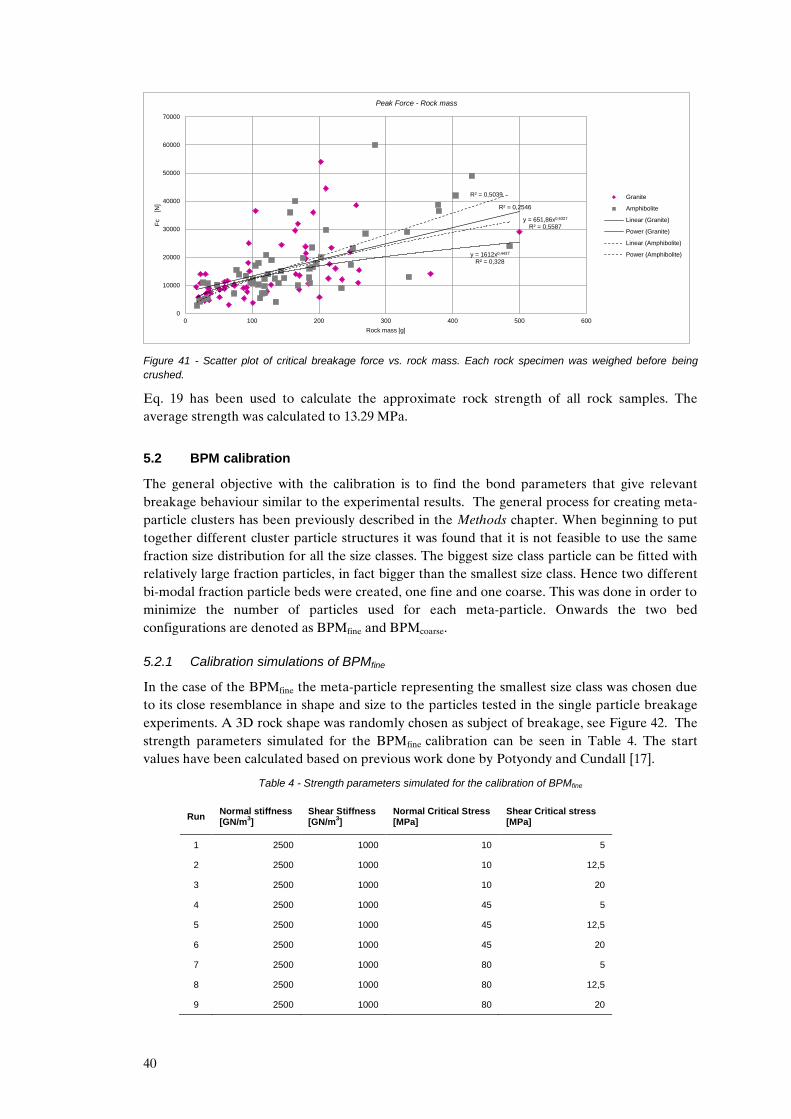
40

Figure 41 - Scatter plot of critical breakage force vs. rock mass. Each rock specimen was weighed before being

crushed.

Eq. 19 has been used to calculate the approximate rock strength of all rock samples. The average strength was calculated to 13.29 MPa.

5.2 BPM calibration

The general objective with the calibration is to find the bond parameters that give relevant breakage behaviour similar to the experimental results. The general process for creating meta-particle clusters has been previously described in the Methods chapter. When beginning to put together different cluster particle structures it was found that it is not feasible to use the same fraction size distribution for all the size classes. The biggest size class particle can be fitted with relatively large fraction particles, in fact bigger than the smallest size class. Hence two different bi-modal fraction particle beds were created, one fine and one coarse. This was done in order to minimize the number of particles used for each meta-particle. Onwards the two bed configurations are denoted as BPMfine and BPMcoarse.

5.2.1 Calibration simulations of BPMfine

In the case of the BPMfine the meta-particle representing the smallest size class was chosen due to its close resemblance in shape and size to the particles tested in the single particle breakage experiments. A 3D rock shape was randomly chosen as subject of breakage, see Figure 42. The strength parameters simulated for the BPMfine calibration can be seen in Table 4. The start values have been calculated based on previous work done by Potyondy and Cundall [17].

Table 4 - Strength parameters simulated for the calibration of BPMfine

Run Normal stiffness [GN/m

3]

Shear Stiffness [GN/m

3]

Normal Critical Stress [MPa]

Shear Critical stress [MPa]

1 2500 1000 10 5

2 2500 1000 10 12,5

3 2500 1000 10 20

4 2500 1000 45 5

5 2500 1000 45 12,5

6 2500 1000 45 20

7 2500 1000 80 5

8 2500 1000 80 12,5

9 2500 1000 80 20

R² = 0,2546

y = 1612x0,4437

R² = 0,328

R² = 0,5039

y = 651,86x0,6327

R² = 0,5587

0

10000

20000

30000

40000

50000

60000

70000

0 100 200 300 400 500 600

Fc [N

]

Rock mass [g]

Peak Force - Rock mass

Granite

Amphibolite

Linear (Granite)

Power (Granite)

Linear (Amphibolite)

Power (Amphibolite)

41

Figure 42 - Pictures of the 3D rock model used in the breakage calibration of BPMfine

In Figure 43 the SPB breakage process can be seen in the DEM environment. The bonds are displayed instead of the fraction particles as it is then easier to observe the crack propagation. The simulation shown is no. 6 and, as can be seen in Figure 44, the particle breaks in two distinct breakage events. The result is a set of progeny particles of various sizes as well as the free fraction particles broken from the main body.

Figure 43 - Snapshots of the calibration breakage simulation of the BPMfine. The pictures shown are a time-sequence

from simulation no. 6 in Figure 44.

For the particle shape chosen the critical force that corresponds to 13.29 MPa is approximately 8000 N. Hence simulation no.5 and no.6 would be possible candidates for a relatively good match.

A lot of tests have been performed in order to reduce the compression ratio at which the breakage occurs. When comparing to the SPB experiments the compression ratios are around one magnitude too high. In order to achieve correct compression ratio the particle and bond stiffness needs to be extremely high. That leads to very small time-steps that are not feasible.

42

Figure 44 - The force-displacement plot for the nine different tested strength combinations simulated for the fine bed

configuration.

5.2.2 Calibration simulations of BPMcoarse

For the BPMcoarse a cylinder has been used as geometry model instead of a 3D scanned rock particle. This shortens the calibration procedure as it is not needed to use the particle replacement functionality. Instead a particle cluster structure is created and bonded together inside a cylinder which is a very simple task to do in EDEM. The same base-file can be used for all the simulations just by changing the bonding strength parameters. Twenty simulations have been performed using batch simulation mode and the settings tested can be seen in Table 5.

Table 5 - Strength parameters simulated for the calibration of BPMcoarse

Run Normal Stiffness [GN/m

3]

Shear Stiffness [GN/m

3]

Normal Critical Stress [MPa]

Shear Critical stress [MPa]

C1 1670 667 45 16

C2 1670 667 45 12

C3 1670 667 45 8

C4 1670 667 45 4

C5 1670 667 45 2

C6 1670 667 45 1

C7 2004 800.4 45 16

C8 2004 800.4 45 12

C9 2004 800.4 45 8

C10 2004 800.4 45 4

C11 2004 800.4 45 2

C12 2004 800.4 45 1

C13 1670 667 30 30

C14 1670 667 33 27

C15 1670 667 36 24

C16 1670 667 39 21

C17 1670 667 42 18

C18 1670 667 45 15

C19 1670 667 48 12

C20 1670 667 51 9

In Figure 45 the cylindrical particle bed is shown as well as the bonds between fraction particles. The picture clearly shows the bi-modal size distribution. If examining the bonding network it

0

2000

4000

6000

8000

10000

12000

14000

0,0% 5,0% 10,0% 15,0% 20,0%

Com

pre

ssiv

e F

orc

e [N

]

Compression ratio [%]

SPB DEM - Force vs. Displacement

1_10x5 [Mpa] 2_10x12,5 [Mpa] 3_10x20 [Mpa]

4_45x5 [Mpa] 5_45x12,5 [Mpa] 6_45x20 [Mpa]

7_80x5 [Mpa] 8_80x12,5 [Mpa] 9_80x20 [Mpa]

43

can be seen that the large fraction particles have a lot of contacts due to the small particles in between. Compared to a mono-size distribution this creates a high level of irregularity and interlocking within the body.

,

Figure 45 - Snapshot from EDEM showing the cylindrical particle bed to the left and the bonds between fraction

particles to the right.

The breakage sequence from one of the calibration simulations can be seen in Figure 46. The force network through the cylindrical bed can clearly be seen. The forces build up until a high enough stress results in crack propagation. One of the problems during the calibration was that, for some of the strength settings, the rock body broke due to local damage only. It was not possible to build up a stress field in the bond network. The bonds in contact with the compression plates could not withhold the local stress. These local damage phenomena can be seen in the fourth picture from the right in Figure 46.

Figure 46 - Snapshots of the calibration breakage simulation of the BPMcoarse. The pictures shown are a time-

sequence from simulation no.C9 in Figure 47.

Figure 47 shows the force-displacement curves for the 20 simulations. It is evident that there is a large output variation. The settings were chosen iteratively by first testing the calculated start values according to the Potyondy and Cundall [17] calculations. Then five new settings were chosen based on the previous results. This iterative process continued until a satisfactory result was obtained. For the cylindrical body the critical force corresponding to ~13.3 MPa is around 95’000 N. Hence the settings chosen for the crusher simulations correspond to simulation C15.

44

Figure 47 - The force-displacement plot for the 20 different tested strength combinations simulated for the coarse bed

configuration.

0

10000

20000

30000

40000

50000

60000

70000

80000

90000

100000

110000

120000

0,0% 2,0% 4,0% 6,0% 8,0% 10,0% 12,0% 14,0% 16,0% 18,0% 20,0%

Com

pre

ssio

n forc

e [N

]

Compression ratio [%]

Force - Displacement for 20 different strength-parameter combinations

C1

C2

C3

C4

C5

C6

C7

C8

C9

C10

C12

C13

C14

C15

C16

C17

C18

C19

C20

45

6. CRUSHER SIMULATION

The aim of this section is to:

- Present results from the performed DEM simulations - Display the capability of the DEM environment in terms of visualization and extraction

of data not possible to measure in real operations

Even though DEM simulations incorporating breakage and BPM models have been performed in previous projects at Chalmers Rock Processing Systems (CRPS) the complexity and ambition in this work have led to difficulties. The process of building BPM models are explained in previous chapters and should be relatively straight forward however there are a lot of things that can go wrong. These problems have occupied a lot of time hence only two out of five simulations have been performed. When the first simulation (CSS34) was started it was found that the computation was too slow. This led to scalping of a large section of the feed material in order to reduce the number of particles.

Table 6 - Simulation parameters for the DEM simulations

Parameter Value Unit

DEM Material properties

Rock Steel

Solid density 2630 7800 [Kg/m3]

Shear stiffness 5.571e8 7e10 [Pa]

Poisson’s ratio 0.35 0.3 [-]

Rock-Rock Rock-Steel

Coefficient of static friction 0.5 0.7 [-]

Coefficient of restitution 0.2 0.25 [-]

Coefficient of rolling friction 0.001 0.001 [-]

BPM parameters

Normal Stiffness 1670 [GN/m3]

Shear Stiffness 667 [GN/m3]

Normal Critical Stress 36 [MPa]

Shear Critical stress 24 [MPa]

Bond disc radius 6.4 [mm]

Machine

Crusher model Svedala H6000 [-]

Chamber type CHX [-]

Eccentric throw 48 [mm]

Eccentric speed 5 [Hz]

Close side setting [34,50] [mm]

Section simulated 1/4 [-]

Liner geometry 3D scanned and modelled [-]

Simulation

Time step 3e-7 [s]

Write out frequency 500 [Hz]

No. of particles (CSS34) 50364 [-]

N0. of particles (CSS50) 92508 [-]

Simulation time (CSS34) 172 [CPUH]

Simulation time (CSS50) 404 [CPUH]

CPU clock freq. 3.33 GHz

CPU cores 8 [-]

Result from the CSS34 simulation was not promising. The particle flow behaviour showed an unrealistic splattering effect with particles exploding during compression. Also, due to the reduced feed batch the chamber never reached choke fed condition.

For the CSS50 simulation two things were changed. In order to get rid of the splattering problem the particle velocity in the simulation was limited to 20m/s and the angular velocity to

46

1200 degrees/s. Sometimes particles overlap too much resulting in very high forces hence high velocities consequently giving a chain reaction. By setting a max velocity in the simulation these unwanted peaks are removed giving a more stable particle flow. The second measure to improve the simulation was to use the whole feed batch originally calculated to fill the chamber.

Settings for both simulations can be seen in Table 6. Comments below generally refer to the CSS50 simulation.

6.1 Particle Flow Behaviour

The flow of particles through the crushing chamber looks realistic compared to observations from experiments. However it is not possible to make live observations of the particle flow during crushing in a choke fed condition. To some degree it is possible to observe rocks that flow and break when the crusher is run empty.

Figure 48 shows meta-particles in the chamber, with each fraction particle coloured by velocity. From the simulations it can be seen that each time a rock particle is captured between the mantle and concave the vertical velocity component either reaches zero or sometimes positive values. The positive velocity component is an effect of the squeezing effect between two planes at an angle. This suggests that the friction between the rock particle and the liner surface is an influential factor for the mass flow through the crusher. This also means that the bulk flow characteristics are important to calibrate in addition to the breakage behaviour. An interesting phenomenon in the discharge region is that particles just leaving the chamber are pushed or thrown away radially by the mantle each time it passes. The rock cascade this results in may explain wear patterns experienced in industrial operations on the walls and supporting beams below the liners. The observed flow behaviour is also supported by the analytical findings by Evertsson [31].

Figure 48 - Snapshot from DEM simulation (CSS50). Particles are coloured according to velocity.

47

6.2 Breakage behaviour

When the mantle rolls over the particle bed a force pulse can be observed with maxima located at the current angular position i.e. the closest gap position. As only a section of the crusher is simulated merely one whole pressure pulse can be observed simultaneously in the particle bed. If simulating the whole crusher it would be possible to see how the pressure pulse travels around the crusher following the mantle motion. From the simulations it can be observed that particles break incrementally due to both interactions between geometries as well as other particles. The population of meta-particles is not entirely broken hence a product size distribution is obtained. A positive result is that the meta-particles are able to break up in progeny particles which are in turn subjected to new breakage events. This shows that the BPM approach not only captures the breakage but is also able to react to different compressive breakage modes. This feature is not yet possible to achieve in PBM breakage models. The PBM approach is based on a threshold force or energy level at which the particle will be replaced with a set of pre-determined progeny particles. This leads to a number of problematic issues and scenarios when using the PBM approach;

1. Particles are not able to respond to different compressive modes. 2. Consider a rock particle compressed at ratio X that leads to an initial crack formation

leading to two main progeny particles. The particle may be further compressed in the same compression event breaking the two progeny particles into a new set of progenies. This type of sequential breakage would be difficult to handle using the PBM approach as the breakage is solely governed by a statistical probability function.

3. For the same compression ratio two particles may break up into a distribution of progeny particles in two distinctly different ways.

Using an impact breakage test as the basis for calculation of threshold values and progeny distributions is wrong since the breakage modes are completely different.

In Figure 49 the numbers of intact bonds in the two simulations are shown. The staircase pattern is of course a result of simulating only a 90 degree section. As can be seen bonds breaks at compression events five times per second. Linear regression gives the bond breakage rate. As previously mentioned the feed batch to the CSS34 simulation was scalped which can be seen from the number of bonds in the beginning of the simulation. These results show a higher breakage rate for CSS50 than CSS34 however this is most likely due to more material in the chamber. Hence no conclusions should be drawn based on these results.

Figure 49 - The plot shows the number of intact particles still in the simulation. The reason for the difference in start

values is due to the different number of meta-particles in the two cases.

y = -52000x + 160190R² = 0,9823

y = -80083x + 314861R² = 0,9968

0

50000

100000

150000

200000

250000

300000

0 0,5 1 1,5 2 2,5 3 3,5 4

No. of in

tact bonds [

-]

Time [s]

No. of intact bonds vs. time

CSS 34 - Number of Intact Bonds CSS 50 - Number of Intact Bonds

Linear ( CSS 34 - Number of Intact Bonds) Linear ( CSS 50 - Number of Intact Bonds)

48

In Figure 50 one compression event is shown through a series of pictures. In the first picture particles are beginning to break. In the third picture the gap is a CSS and a lot of broken bonds are displayed as black vectors. In the subsequent pictures the mantle rolls over and in the last pictures the particles are free to fall due to gravity.

Figure 50 - The series of pictures displays one compression event. The meta-particles are shown as bonds colourer

according to perceived normal force.

In order to calculate the pressure from the DEM simulation the force response on the mantle has been extracted. The total force magnitudes as well as the z-components over time are shown in Figure 51. A large difference can be observed between the two simulations. The reason is the lack of feed material in the CSS34 case. Focusing on the CSS50 simulation it shows that a substantial part of the force between particles and the mantle is accounted for by the z-component. It would be very interesting to see what the shape of the force response is when

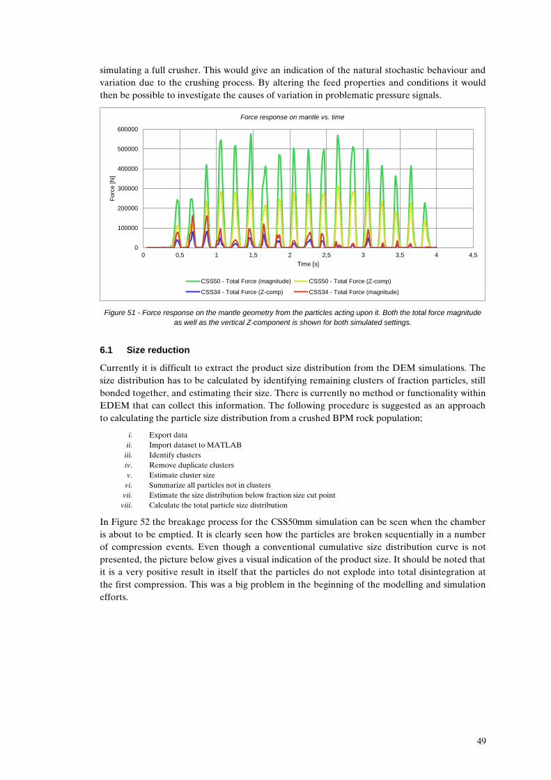
49

simulating a full crusher. This would give an indication of the natural stochastic behaviour and variation due to the crushing process. By altering the feed properties and conditions it would then be possible to investigate the causes of variation in problematic pressure signals.

Figure 51 - Force response on the mantle geometry from the particles acting upon it. Both the total force magnitude

as well as the vertical Z-component is shown for both simulated settings.

6.1 Size reduction

Currently it is difficult to extract the product size distribution from the DEM simulations. The size distribution has to be calculated by identifying remaining clusters of fraction particles, still bonded together, and estimating their size. There is currently no method or functionality within EDEM that can collect this information. The following procedure is suggested as an approach to calculating the particle size distribution from a crushed BPM rock population;

i. Export data ii. Import dataset to MATLAB

iii. Identify clusters iv. Remove duplicate clusters v. Estimate cluster size

vi. Summarize all particles not in clusters vii. Estimate the size distribution below fraction size cut point

viii. Calculate the total particle size distribution

In Figure 52 the breakage process for the CSS50mm simulation can be seen when the chamber is about to be emptied. It is clearly seen how the particles are broken sequentially in a number of compression events. Even though a conventional cumulative size distribution curve is not presented, the picture below gives a visual indication of the product size. It should be noted that it is a very positive result in itself that the particles do not explode into total disintegration at the first compression. This was a big problem in the beginning of the modelling and simulation efforts.

0

100000

200000

300000

400000

500000

600000

0 0,5 1 1,5 2 2,5 3 3,5 4 4,5

Fo

rce

[N

]

Time [s]

Force response on mantle vs. time

CSS50 - Total Force (magnitude) CSS50 - Total Force (Z-comp)

CSS34 - Total Force (Z-comp) CSS34 - Total Force (magnitude)

50

Figure 52 - Snapshot from EDEM showing the breakage process. The fraction particles are hidden and only the

bonds, coloured according to perceived normal force, are shown. When bonds are broken they change colour to

black. The black broken bonds appear in the visualization as long as the two bonded particles are still within 10mm

from each other.

In Figure 53 two pictures are shown at the same time-step. In the picture to the left the meta-particles are visually represented by the bonds and on the right the fraction particles are displayed. Both ways of displaying the breakage process are interesting and have their own advantage. When displaying only the bonds it is easier to see the actual breakage events and the new progeny clusters that form post breakage. When displaying particles the free fractions broken apart from the clusters are also seen. Due to the large amount of particles it is difficult to see the actual breakage however it gives a better understanding of the particle flow in the chamber. Also, when displaying the bonds it looks like the bulk density in the chamber is reduced when travelling downwards through the chamber. It can clearly be seen that this is not the case when displaying the fractions. Of course the reason for this is that more bonds are broken the further down the chamber resulting in more free fractions in between the unbroken clusters.

51

Figure 53 - Snapshot from EDEM showing the breakage process. In the left hand picture the particles are visualized

by the bonds and in the right hand picture the fraction particles are displayed.

52

7. RESULTS & DISCUSSION

The aim of this section is to:

- Make a comparative study between the experiments and simulations - Discuss the level of compliance between the two domains

7.1 Hydrostatic Pressure

A comparison of the hydrostatic pressure between simulation and experiments can be seen in Figure 54. The experimental data displays four seconds of operation randomly chosen from the data set. The simulation data corresponds to the accumulated z-component forces acting on the mantle for every time position. The total vertical force is divided by the bearing area in order to calculate the pressure. Also, the mass of the main shaft package has been accounted for by estimating the masses of all main shaft package components using the CatiaV5 CAD model.

As only a 90 degree section has been modelled the pressure signal from the simulation is different to the experiment. If modelling the full crusher the DEM pressure signal would have less variation. With this in mind it is interesting that the results comply as well as they do. Spikes appear according to the eccentric frequency in both experiment and simulation. This provides further evidence to the hypothesis that the feeding conditions in the experiments have been segregated and misaligned.

Figure 54 – Hydrostatic pressure comparison between simulation and experiment for CSS 50mm.

7.2 Throughput Capacity

A comparison of the throughput capacity between simulation and experiment can be seen in Figure 55. The experimental data is directly taken from Figure 29. In the case of the simulation a few things needs to be accounted for such as the sectioning and BPM bulk density. Hence the expression in Eq. 20 is used for calculating the total throughput capacity.

0

0,5

1

1,5

2

2,5

3

3,5

0 0,5 1 1,5 2 2,5 3 3,5 4 4,5

Pre

ssure

[M

Pa]

Time [S]

Pressure CSS50 - Experiment vs. DEM

DEM - CSS50 - Pressure [MPa] EXP - CSS50 - Pressure [MPa]

53

Eq. 20

Where is the mass flow rate in the discharge region, is the sectioning factor, is the

bulk density of the BPM clusters and is a factor that accounts for the feed size distribution cut off point i.e. the amount of small particles that are not modelled in the feed.

The results show a good conformation between simulation and experimental results. This was expected for the CSS50 simulation due to the higher amount of feed material and more stable operation. However it is surprising that the CSS34 data corresponds as well as it does.

Figure 55 – Throughput capacity comparison between simulations and experiments for CSS 34 mm and CSS 50 mm.

The error bars for the DEM columns represent the standard deviation of the mass flow rate data. The error bars for

the experimental columns represent a 5% deviation (subjectively estimated) due to e.g. belt speed deviation or

sample processing error.

When measuring crusher capacity it is normally important to consider how much of a specific product size that is being produced. This is called the production yield. In the aggregate industry it is often more important to produce as much as possible of the currently most lucrative product than to maximize total throughput capacity. As the method for calculating the product particle size distribution is not developed yet it is currently not possible to obtain the product yield data from the simulations. When this is available it will potentially be possible to optimize liner design as well as the operational setting towards specific production targets. More importantly it may be possible to, from observing the simulations, understand that breakage and flow behaviour leads to the wanted targets. This kind of understanding will in turn enable increased accuracy of the analytical mechanistic cone crusher models.

7.3 Power draw

In Figure 56 the power draw is shown for both experiment and simulation at CSS 50mm. As can be seen the peaks are much higher in the simulation case than the experiment case. Coincidently the average power draw matches fairly well in the graph however the quarter sectioning is not accounted for hence the DEM simulations over predict with a factor of four. From the DEM simulations the power draw is obtained by calculating the total torque on the mantle due to the tangential forces exerted by the rock particles on the mantle. This method of calculating the power draw needs to be overlooked as it seems not to give a good indication of the power draw. Currently the estimation of the total torque upon the mantle is calculated and exported by EDEM. An alternative approach would be to export every individual rock particle-mantle force vector and perform the entire analysis in MATLAB instead. This would rule out

0

50

100

150

200

250

300

350

400

450

500

Th

roughput

Capacity [to

n/h

]

Throughput capacity - DEM vs. Experiment

CSS34 - DEM

CSS34 - EXP

CSS50 - DEM

CSS50 - EXP

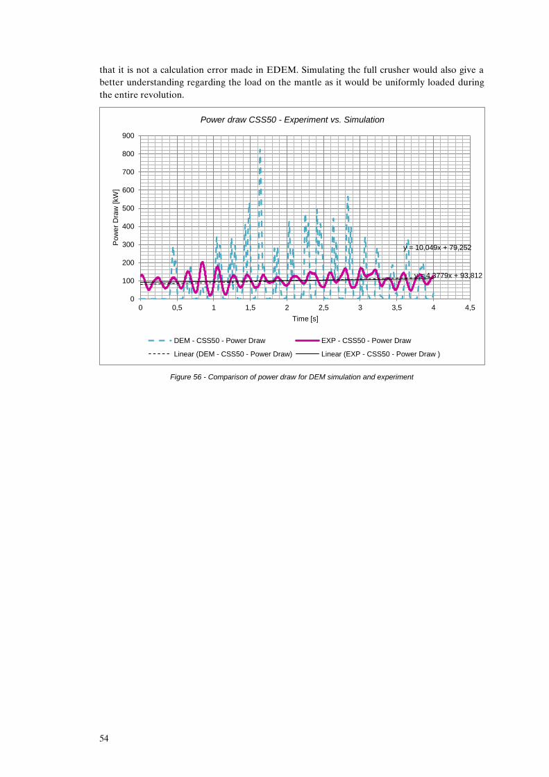
54

that it is not a calculation error made in EDEM. Simulating the full crusher would also give a better understanding regarding the load on the mantle as it would be uniformly loaded during the entire revolution.

Figure 56 - Comparison of power draw for DEM simulation and experiment

y = 10,049x + 79,252

y = 4,3779x + 93,812

0

100

200

300

400

500

600

700

800

900

0 0,5 1 1,5 2 2,5 3 3,5 4 4,5

Pow

er

Dra

w [

kW

]

Time [s]

Power draw CSS50 - Experiment vs. Simulation

DEM - CSS50 - Power Draw EXP - CSS50 - Power Draw

Linear (DEM - CSS50 - Power Draw) Linear (EXP - CSS50 - Power Draw )

55

8. CONCLUSIONS

The aim of this section is to:

- Draw conclusion regarding the validation of the developed DEM crusher model - Answer the previously stated research questions

This master thesis work has generated results and outcome in different knowledge domains. First of all a virtual crushing environment has been developed and can now be used as a novel simulation tool. Secondly the performed experiments and simulations contribute to the general understanding regarding cone crusher performance.

The project was conducted over a longer time period due to several reasons. However, most of the initially stated tasks and goals of the project have been performed even though some were relatively difficult to achieve.

Since only one quality simulation has been performed it is not possible to draw conclusions regarding the validation apart from this specific case. The CSS 50 mm simulation looks very promising in terms of flow behaviour and breakage process visually. The other CSS setting needs to be simulated in the same setup in order to draw full conclusions regarding validation.

In order to evaluate if the objectives stated in the early phases have been achieved each research question will be commented on below;

RQ1. How should a modelling and simulation environment be designed in order to effectively evaluate performance and design of cone crushers?

When using the virtual crushing environment for design evaluation it is preferable to have as low setup time as possible. If the purpose of the simulation is to evaluate e.g. a new liner design it is possible to just replace the old geometry with the new and reuse all other settings. It would be possible to put in an initial effort to make base models of e.g. all of the crusher models within the product portfolio. The time required to setup a specific simulation is then substantially reduced. Of course one would think that a fully automated simulator would be preferable. However, due to the complexity of the model it is a potential risk if all of the details and limitations of the simulator are not fully understood.

It would be preferable to predefine a large number of meta-particle models to choose from in order to enable an easy assembly of the rock population. When a material model has been developed and calibrated it can of course be reused for later projects. A library of calibrated BPM models would be a very good feature.

If performing crusher simulations on a regular basis the post processing needs to be more automated. Currently the data is exported manually to MATLAB or MS Excel where a lot of manual work is done in order to convert the data to valuable information.

RQ2. To what extent is it possible to use DEM for predicting crusher performance?

The presented results suggest that the performance can be predicted in a good way when it comes to mass flow and pressure. More work has to be performed on the post-processing in order to be able to draw conclusions regarding size distribution and power draw.

RQ3. How should a DEM simulation properly be calibrated in order to comply with real behaviour?

In this work single particle breakage tests have been successfully used as the basis for calibration. The approach of using SPB and not uniaxial strength test or Brazilian test gave a lot of insight regarding the influence of compression mode. The standardized breakage tests generate more statistically predictable data however they do not really capture the complex

56

breakage of irregular particles with flaws and sharp corners. In future work interparticle piston and die tests will be evaluated as a suitable method for calibration. Potentially the best result is gained if conducting both uniaxial strength tests as well as SPB and IPB tests.

The simulation approaches for finding corresponding settings that give good breakage behaviour have been semi-systematic in this work. Based on the experience from this work a more statistical approach should be applied. By using the statistical method design of experiments (DoE) for choosing settings and utilizing batch simulation mode, the correct strength parameters can be found more efficiently. It would be interesting to develop a calibration procedure where the data from one simulation is processed and used in an optimization algorithm for choosing the next set of values.

RQ4. What level of accuracy can be reached by using DEM for simulation of existing cone crushers?

This question is difficult to answer however from the work it can be concluded that it is all about trade-offs. It is possible to model and simulate a small section of a crusher very accurately in terms of capturing most of the size distribution. However, the material model quality suffers greatly if the full crusher should be modelled. Currently more computational power is needed in order to simulate a full continuous cone crusher operation with a good material model.

The computational time for the CSS50 simulation was around 400 hours and the number of particles was 92500. This is enough for filling the chamber to a fairly good choke fed condition momentarily. Hence if feeding and discharging continuously, only slightly more particles are needed in order to obtain steady state condition. This leads to the conclusion that in order to model the full crusher in steady state we need to use 300-400K particles which would give a simulation time of around 1365 hours or 57 days, which is not feasible. Simulating a full crusher using this methodology hence requires a computational capacity scale up by at least a factor of 3-6.

RQ5. How does a change in close side setting influence the internal particle dynamics and crushing operation in the crushing chamber?

If considering both results from experiments and simulations, there is an indication that when increasing the close side setting the,

throughput capacity increases power draw decreases linearly hydrostatic pressure decreases linearly particle size distribution gets coarser reduction ratio decreases

57

9. FUTURE WORK

The aim of this section is to:

- make recommendations to future work in order to bridge the problems observed in the project

- make recommendations on what to focus on in the future development of DEM crusher models

Even though a substantial set of parameters and conditions have been captured in the DEM model there are a number of critical aspects that need further improvement;

1. Batch feed - Due to computational intensity restrictions only a relatively small batch size has been simulated. In order to be able to model more material a higher computational capacity is needed. Also a slightly different approach is needed for introducing the meta-particles in a continuous manner.

2. Sectioning - Due to computational economy only a 90° section of the crusher has been modelled. Of course it would be preferable to model the full crusher.

3. Packing density – Due to the packing density in the BPM there is a problem with mass conservation.

During the late phases of the project a new meta-particle replacement method was developed. It was not possible to test it in this work however this will solve the issue of not being able to use the full rock population that was developed.

In this work the built in bonded particle model in EDEM has been used. It is also possible to write a customized mode by altering source code published by EDEM. This will enable better control of the strength distribution and other BPM aspects.

Efforts need to be put into developing the post-processing in order to capture product particle size distribution and power draw in a better way.

58

10. REFERENCES

1. Whiten, W.J., The Simulation of Crushing Plants with Models Developed using Multiple Spline

Regression. J. SAIMM, 1972. 072(10): p. 257-264.

2. Eloranta, J., Influence of Crushing Process Variables on the Product Quality of Crushed Rock,

1995, Tampere University of Technology: Tampere.

3. Evertsson, C.M., Cone Crusher Performance, in Dep. of Machine and Vehicle Design2000,

Chalmers University of Technology: Göteborg.

4. Bengtsson, M., Quality-Driven Production of Aggregates in Crushing Plants, in Dep. Product

and production Development2009, Chalmers University of Technology: Gothenburg, Sweden.

5. Hulthén, E. and C.M. Evertsson, Algorithm for dynamic cone crusher control. Minerals

Engineering, 2009. 22(3): p. 296-303.

6. Hulthén, E., Real-Time Optimization of Cone Crushers, in Dep. Product and Production

Development2010, Chalmers University of Technology: Göteborg.

7. Quist, J.C.E., Evertsson, C.M. Application of discrete element method for simulating feeding

conditions and size reduction in cone crushers. in XXV INTERNATIONAL MINERAL

PROCESSING CONGRESS. 2010. Brisbane, QLD, Australia.

8. Lichter, J., et al., New developments in cone crusher performance optimization. Minerals

Engineering, 2009. 22(7-8): p. 613-617.

9. Djordjevic, N., F.N. Shi, and R.D. Morrison, Applying discrete element modelling to vertical

and horizontal shaft impact crushers. Minerals Engineering, 2003. 16(10): p. 983-991.

10. Schubert, W., Jeschke, H. DEM-simulation of the Breakage Process in an Impact Crusher.

New Orders of the Comminution, 2005. 4.

11. Quist, J.C.E., Evertsson, C.M., Simulating Capacity and Breakage in Cone Crushers Using

DEM, in Comminution 10'2010: Capetown, South Africa.

12. Quist, J.C.E., Evertsson, C.M., Franke, J., The effect of liner wear on gyratory crushing – a

DEM case study, in Computational Modeling 11'2011: Falmouth.

13. DEM-Solutions, EDEM 2.4 Theory Reference Guide, 2011, DEM Solutions: Edinburgh.

14. Hertz, H., Ueber die Beruehrung elastischer Koerper (On Contact Between Elastic Bodies), in

Gesammelte Werke (Collected Works)1882: Leipzig, Germany.

15. Mindlin, R.D., Complience of elastic bodies in contact. Journal of Applied Mechanics, 1949.

16: p. 259-268.

16. Quist, J.C.E. Device for calibration of DEM contact model parameters. in EDEM Conference

11'. 2011. Edinburgh.

17. Potyondy, D.O. and P.A. Cundall, A bonded-particle model for rock. International Journal of

Rock Mechanics and Mining Sciences, 2004. 41(8): p. 1329-1364.

18. Cho, N., C.D. Martin, and D.C. Sego, A clumped particle model for rock. International Journal

of Rock Mechanics and Mining Sciences, 2007. 44(7): p. 997-1010.

19. Cundall, P.A., Strack, O.D., A discrete numerical model for granular assemblies.

Géotechnique, 1979. 29(1): p. 47-65.

20. Schönert, K., A first survey of grinding with high-compression roller mills. International

Journal of Mineral Processing, 1988. 22(1–4): p. 401-412.

21. Tavares, L.M., Chapter 1 Breakage of Single Particles: Quasi-Static, in Handbook of Powder

Technology, M.G. Agba D. Salman and J.H. Michael, Editors. 2007, Elsevier Science B.V. p.

3-68.

22. Hiramatsu, Y. and Y. Oka, Determination of the tensile strength of rock by a compression test

of an irregular test piece. International Journal of Rock Mechanics and Mining Sciences

&amp; Geomechanics Abstracts, 1966. 3(2): p. 89-90.

59

23. Briggs, C., Evertsson, C.M., Shape Potential Of Rock. Minerals Engineering, 1998. 11(2): p.

125-132.

24. Liu, J. and K. Schönert, Modelling of interparticle breakage. International Journal of Mineral

Processing, 1996. 44–45(0): p. 101-115.

25. Schönert, K., The influence of particle bed configurations and confinements on particle

breakage. International Journal of Mineral Processing, 1996. 44–45(0): p. 1-16.

26. Khanal, M., W. Schubert, and J. Tomas, Discrete element method simulation of bed

comminution. Minerals Engineering, 2007. 20(2): p. 179-187.

27. Couroyer, C., Z. Ning, and M. Ghadiri, Distinct element analysis of bulk crushing: effect of

particle properties and loading rate. Powder Technology, 2000. 109(1–3): p. 241-254.

28. Liu, H.Y., S.Q. Kou, and P.A. Lindqvist, Numerical studies on the inter-particle breakage of a

confined particle assembly in rock crushing. Mechanics of Materials, 2005. 37(9): p. 935-954.

29. Bergman, B., Klefsjö, B., Quality from Customer Needs to Customer Satisfaction. Vol. 3.

2010, Sweden: Studentlitteratur AB. 654.

30. Smallman, R.E., Ngan, A.H.W., Physical Metallurgy and Andvanced Materials. Seventh

edition ed2007, Oxford: Elsevier.

31. Evertsson, C.M., Modelling of flow in cone crushers. Minerals Engineering, 1999. 12(12): p.

1479-1499.