concept of (dis)similarity in data analysis

Trends Trends in Analytical Chemistry, Vol. 38, 2012

Concept of (dis)similarity in dataanalysisPiotr Zerzucha, Beata Walczak

(Dis)similarity matrices (the Euclidean distance matrix included) can be used for unsupervised and supervised data analysis. In

this review, we use four different data sets (real and simulated, with different dimensionalities and a different correlation

structure) to demonstrate the performance of dissimilarity-based approaches [e.g., hierarchical clustering, dissimilarity-Partial

Least Squares (dissimilarity-PLS) and Non-parametric Multiple Analysis of Variance (NP-MANOVA)].

Dissimilarity-PLS performs well for linear and highly non-linear data, both in regression and discrimination settings.

NP-MANOVA allows for a fast randomization test of the statistical significance of the factors studied in the designed experiments.

Dissimilarity-based approaches can be applied to data sets with numerous variables. However, if the studied data set contains

numerous objects, a full dissimilarity matrix should be replaced with a dissimilarity matrix containing the distances of all of the

objects to preselected ‘‘prototypes’’. Although we focus on the Euclidean distance, any dissimilarity measure can be used in the

approaches discussed, thus enlarging the areas of their application to different types of variable (e.g., nominal variable, and

sensory data).

ª 2012 Elsevier Ltd. All rights reserved.

Keywords: Analysis of variance (ANOVA); Data analysis; (Dis)similarity; Dissimilarity-Partial Least Squares (dissimilarity-PLS); Hierarchical

clustering; Nominal variable; Non-linear discrimination; Non-linear regression; Non-parametric Multiple Analysis of Variance (NP-MANOVA);

Sensory data

Piotr Zerzucha,

Beata Walczak*

Institute of Chemistry,

The University of Silesia,

Szkolna Street 9, 40-006

Katowice, Poland

*Corresponding author.

E-mail: [email protected]

116

1. Introduction

There are two common ways of data rep-resentation in data analysis, vectorial(based on features) and pairwise (based onrelations).

1.1. Pairwise representationPairwise representation is popular in somefields (e.g., bioinformatics, cognitive psy-chology, social sciences, text and webmining) [1–5], but it is rarely used inchemistry.

The basic concept explored in pairwiserepresentation is the concept of similarityor dissimilarity. Because each similarityfunction can be converted into a dissimi-larity function, further in this text, we willuse the terms ‘‘similarity’’ and ‘‘dissimi-larity’’ interchangeably. The concept ofsimilarity is more general than the conceptof metric distances. Distance d, represent-ing the dissimilarity of x and y objects, isconsidered to be a metric distance if it hasthe following properties:(1) positivity, i.e. d(x,y) > 0, if x is dis-

tinct from y(2) reflectivity, i.e. d(x,x) = 0

0165-9936/$ - see front matter ª 2012 Elsevier Ltd. All rights

(3) symmetry, i.e. d(x,y) = d(y,x)(4) triangle inequality, i.e. d(x,y) 6

d(x,z) + d(z,y) for each zA dissimilarity matrix usually satisfies

the reflectivity condition (2), often satisfiesthe positivity condition (1), sometimesfulfills symmetry condition (3) and rarelysatisfies the triangle-inequality condition(4) [6].

If only pairwise data is available for dataanalysis, there are at least three possibleways of dealing with the lack of vectorialrepresentation.

1.1.1. Low-dimensional embedding: Multidi-mensional scaling. In the areas wherepairwise representation dominates, a greatamount of effort is devoted to studies onhow to pass from pairwise to vectorial rep-resentation. In the other words, multidi-mensional scaling attempts to find anembedding from the pairwise representa-tion to the RN space, such that the distancesare preserved. If N is selected as 2 or 3, thestudied objects can be visualized in the R2

or R3 space, respectively. The proximity ofobjects to each other indicates how similarthese objects are. For Euclidean pairwise

reserved. doi:http://dx.doi.org/10.1016/j.trac.2012.05.005

http://dx.doi.org/10.1016/j.trac.2012.05.005

Trends in Analytical Chemistry, Vol. 38, 2012 Trends

data, the problem is easy, because a set of vectors exists ina Euclidean space so that the mutual distances betweenthe vectors are the same, as for the pairwise data. How-ever, for a general type of pairwise data (which are usuallynon-Euclidean), this translation is impossible and otherapproaches (e.g., approximation or unification) have beendeveloped [7]. They allow samples to be embedded into aEuclidean space that is then followed by standard methodsof data analysis.

1.1.2. Modification of similarities into kernels. Anotherapproach eliminates the necessity of explicitly embed-ding the samples into a Euclidean space. Namely, themetric distance matrices can be treated as kernels andused in kernel-based methods, and the non-metricsimilarity matrices can be converted into positive definitekernels and also used in kernel machines. A popularapproach for dealing with non-positive definite similaritymatrices is to transform the spectrum of a similaritymatrix so as to generate a positive definite kernel matrix.Among the proposed methods are denoise, flip, diffusion,shift or spectrum square [8]. The interest in methods ofmodifying dissimilarity matrices into kernels is associ-ated with the fact that the positive definite kernels allowall the concepts of reproducing kernel Hilbert space to beused [9].

1.1.3. Algorithmic approach. Another possibility is theso-called algorithmic approach, which allows similaritiesto be treated as new features and as input for the simi-larity-based methods [10] that depend on inner productsonly. If an indefinite similarity matrix is an input to, e.g.,the Support Vector Machine (SVM), the SVM problemwill no longer be convex, but – as demonstrated by Linand Lin [11] – a simple modification of the originalalgorithm assures its convergence (although the solutionis a stationary point instead of a global minimum).

1.2. From vectorial to pairwise representationThe vectorial representation of data dominates in chem-istry because it is well suited to all the data-analysismethods. However, we can always translate this type ofdata into a pairwise representation using a problem-dependent similarity measure (metric or non-metric).The main goal of this translation type is that a pairwiserepresentation captures the structure that is not capturedby the vectorial data [1,12]. Until now, this approach hasnot been popular in chemometrics because, by transfer-ring vectorial data into a pairwise representation, we losethe possibility of interpreting the influence of the indi-vidual features on the phenomenon studied. However,with the increasing number of applications of chemo-metrics for bio-systems studies, there is an increasingneed for effective tools that are able to deal with non-linear problems.

So far, non-linear problems have been dealt withmainly using Neural Networks or the SVMs methods[13–16]. However, a closer look at the published appli-cations of SVMs in chemometrics reveals that only a fewtypes of kernel are extensively used, namely, Gaussianand polynomial [17]. The same kernels are also used inother kernel-based methods {e.g., kernel-Linear Dis-criminant Analysis (kernel-LDA) or kernel-Partial LeastSquares (kernel-PLS) [18–21]}. These kernel functionsare continuous, symmetric and have a positive definiteGram matrix. They satisfy Mercer�s theorem [22] be-cause they are definite (i.e. their kernel matrices have nonon-negative eigenvalues). The requirement of a positivedefinite kernel in kernel-based methods is associatedwith the fact that these properties ensure that the opti-mization problem will be convex and the solution will beunique. There is, however, a large class of kernels thatare not positive definite (the so-called conditionally po-sitive definite) that can be used as generalized distances[23]. They have the following form:

kðxi; xjÞ ¼ �jjxi � xjjjp; 0 < p < 2 ð1ÞMoreover, there are many algorithms that can be used

directly with the different types of similarity matrices. Withcommon chemometrics methods [e.g., Principal Compo-nent Regression (PCR) or Partial Least Squares (PLS)], wecan treat pairwise representation as a new feature repre-sentation and perform modeling directly on it.

Although we lose certain information when changingvectorial representation into pairwise representation[24], we demonstrate in this article that pairwise rep-resentation reveals a data structure (which is not re-vealed in the vectorial data representation) and can beused for modeling highly non-linear data.

1.3. Dissimilarity measureThere are many dissimilarity/similarity measures (e.g.,Euclidean, Mahalanobis, Manhattan distances, andsquared Euclidean distance – see Table 1) that can beused for the comparison of objects studied in the space ofmeasured variables [25].

If we intend to compare m objects simultaneously,each described by n parameters, the dissimilarity be-tween each pair of objects can be organized in the formof a square and symmetric matrix D of dimensionality(m x m). This dissimilarity matrix can be used in manyinteresting applications. It can be considered as anexample of the so-called conditionally positive-definitekernel [26] and it can be used in all kernel-based ap-proaches (e.g., SVMs).

In this review, we present the most popular and themost attractive applications of dissimilarity matrices inchemometrics. Although we limit ourselves to Euclideandistance as a dissimilarity measure, it should be stressedthat each type of dissimilarity/similarity measure canfind analogous applications.

http://www.elsevier.com/locate/trac 117

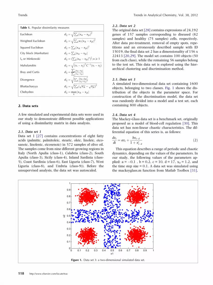
Table 1. Popular dissimilarity measures

Euclidean dij ¼ffiffiffiffiffiffiffiffiffiffiffiffiffiffiffiffiffiffiffiffiffiffiffiffiffiffiffiffiffiffiffiP

k ðxik � xjk Þ2q

Weighted Euclidean dij ¼ffiffiffiffiffiffiffiffiffiffiffiffiffiffiffiffiffiffiffiffiffiffiffiffiffiffiffiffiffiffiffiffiffiffiffiffiffiP

k wiðxik � xjkÞ2q

Squared Euclidean dij ¼P

k ðxik � xjk Þ2

City block (Manhattan) dij ¼P

k jxik � xjk j

la or Minkowski dij ¼ ðP

k jxik � xjk jaÞ1a; a P 1

Mahalanobis dij ¼ffiffiffiffiffiffiffiffiffiffiffiffiffiffiffiffiffiffiffiffiffiffiffiffiffiffiffiffiffiffiffiffiffiffiffiffiffiffiffiffiffiffiffiffiffiffiffiðxi � xjÞT C�1ðxi � xjÞ

q

Bray and Curtis dij ¼P

kjxik�xjk jP

kðxik�xjk Þ

Divergence dij ¼ffiffiffiffiffiffiffiffiffiffiffiffiffiffiffiffiffiffiffiffiffiffiffiffiP

kðxik�xjk Þ2

ðxikþxjk Þ2

r

Bhattacharyya dij ¼ffiffiffiffiffiffiffiffiffiffiffiffiffiffiffiffiffiffiffiffiffiffiffiffiffiffiffiffiffiffiffiffiffiffiffiffiffiffiffiP

k ðffiffiffiffiffiffixikp � ffiffiffiffiffiffi

xjkp Þ2

q

Chebyshev dij ¼ maxkjxik � xjk j


2. Data sets

A few simulated and experimental data sets were used inour study to demonstrate different possible applicationsof using a dissimilarity matrix in data analysis.

2.1. Data set 1Data set 1 [27] contains concentrations of eight fattyacids (palmitic, palmitoleic, stearic, oleic, linoleic, eico-sanoic, linolenic, eicosenoic) in 572 samples of olive oil.The samples come from nine different growing regions inItaly (North Apulia (class-1), Calabria (class-2), SouthApulia (class-3), Sicily (class-4), Inland Sardinia (class-5), Coast Sardinia (class-6), East Liguria (class-7), WestLiguria (class-8), and Umbria (class-9)). Before theunsupervised analysis, the data set was autoscaled.

0 0.1 0.2 0.3 0.4 00

0.1

0.2

0.3

0.4

0.5

0.6

0.7

0.8

0.9

1

x

x2

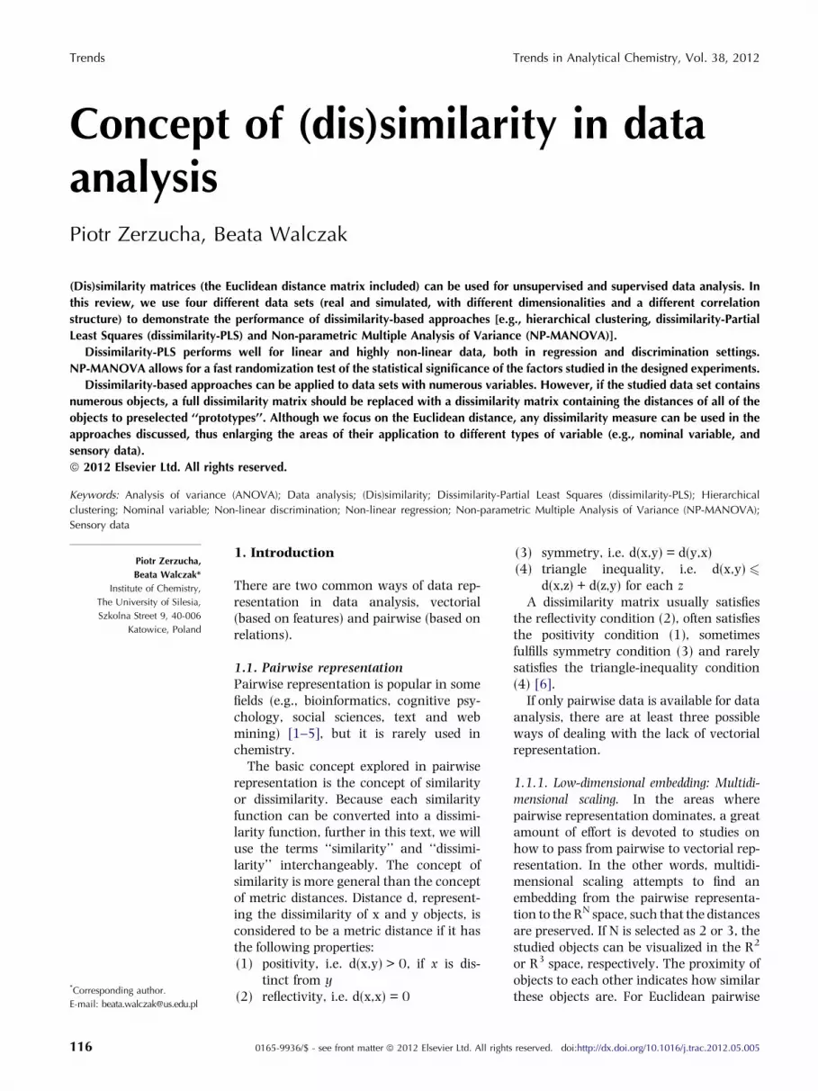
Figure 1. Data set 3: a two-dime

118 http://www.elsevier.com/locate/trac

2.2. Data set 2The original data set [28] contains expressions of 24,192genes of 157 samples corresponding to diseased (82samples) and healthy (75 samples) cells, respectively.After data pre-treatment, removal of empty spots, repe-titions and an erroneously described sample with ID15019, the final data set 2 has a dimensionality of 156 x22413 [20,29]. The model set contains 100 objects (50from each class), while the remaining 56 samples belongto the test set. This data set is explored using the hier-archical clustering and discrimination method.

2.3. Data set 3A simulated two-dimensional data set containing 1600objects, belonging to two classes. Fig. 1 shows the dis-tribution of the objects in the parameter space. Forconstruction of the discrimination model, the data setwas randomly divided into a model and a test set, eachcontaining 800 objects.

2.4. Data set 4The Mackey-Glass data set is a benchmark set, originallyproposed as a model of blood-cell regulation [30]. Thisdata set has non-linear chaotic characteristics. The dif-ferential equation of this series is, as follows:

dxt

dt¼ axt þ

bxt�d

1þ xct�d

ð2Þ

This equation describes a range of periodic and chaoticdynamics, depending on the values of the parameters. Inour study, the following values of the parameters ap-plied: a = �0.1 , b = 0.2, c = 10, d = 17, x0 = 1.2, andthe time step size = 0.1. A data set was simulated usingthe mackeyglass.m function from Matlab Toolbox [31],

.5 0.6 0.7 0.8 0.9 11

nsional simulated data set.


in which the 4th order Runge-Kutta integration methodis applied. The model set contains 3000 (first) samples,whereas the test set contains 2000 consecutive samples.Each sample is described by the following independentvariables x(t), x(t�1), . . . , x(t�15) and the dependent(described output) is given by x(t+prediction horizon),where the prediction horizon is set to 1, 5, or 10. In ourstudy, the noise-free and noisy data (10% of the datastandard deviation) were modeled.

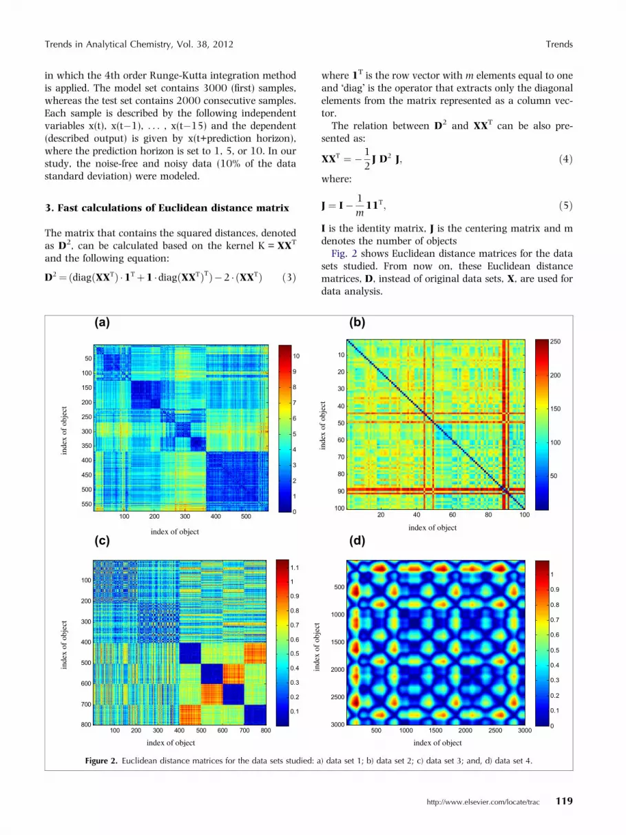
3. Fast calculations of Euclidean distance matrix

The matrix that contains the squared distances, denotedas D2, can be calculated based on the kernel K = XXT

and the following equation:

D2¼ðdiagðXXTÞ �1Tþ1 �diagðXXTÞTÞ�2 � ðXXTÞ ð3Þ

100 200 300 400 500 600 700 800

100

200

300

400

500

600

700

800

0.1

0.2

0.3

0.4

0.5

0.6

0.7

0.8

0.9

1

1.1

100 200 300 400 500

50

100

150

200

250

300

350

400

450

500

5500

1

2

3

4

5

6

7

8

9

10

(a)

(c)

index of object

index of object

inde

x of

obj

ect

inde

x of

obj

ect

Figure 2. Euclidean distance matrices for the data sets studied: a

where 1T is the row vector with m elements equal to oneand �diag� is the operator that extracts only the diagonalelements from the matrix represented as a column vec-tor.

The relation between D2 and XXT can be also pre-sented as:

XXT ¼ �1

2J D2 J; ð4Þ

where:

J ¼ I� 1

m11T; ð5Þ

I is the identity matrix, J is the centering matrix and mdenotes the number of objects

Fig. 2 shows Euclidean distance matrices for the datasets studied. From now on, these Euclidean distancematrices, D, instead of original data sets, X, are used fordata analysis.

20 40 60 80 100

10

20

30

40

50

60

70

80

90

100

50

100

150

200

250

500 1000 1500 2000 2500 3000

500

1000

1500

2000

2500

3000 0

0.1

0.2

0.3

0.4

0.5

0.6

0.7

0.8

0.9

1

(b)

(d)

inde

x of

obj

ect

index of object

index of object

inde

x of

obj

ect

) data set 1; b) data set 2; c) data set 3; and, d) data set 4.



4. Data clustering

The main goal of data-clustering methods is to divide thesamples studied into groups of similar samples. Whenthe number of groups is unknown a priori, the data-clustering tendency can be studied using hierarchicalclustering methods [32–36]. Hierarchical clustering(and any other type of clustering) can be performed di-rectly on distance matrix D.

In so-called agglomerative hierarchical clusteringmethods, individual objects are merged together pro-gressively based on their distance (or similarity). Thearrangement of the clusters produced by hierarchicalclustering is usually presented in the form of a treediagram, called a dendrogram. Given the distancematrix, D (m x m), the basic steps of hierarchicalclustering are as follows:(1) Each object is assigned to a cluster (if there are m

objects, there are m clusters).(2) The closest (similar) pair of clusters is merged into a

single cluster (total number of clusters in now onecluster less).

(3) Distances between the new cluster and each of theold clusters are computed.

(4) Steps 2 and 3 are repeated until all objects are clus-tered into a single cluster (containing m objects).

The linkage criterion determines the distance between
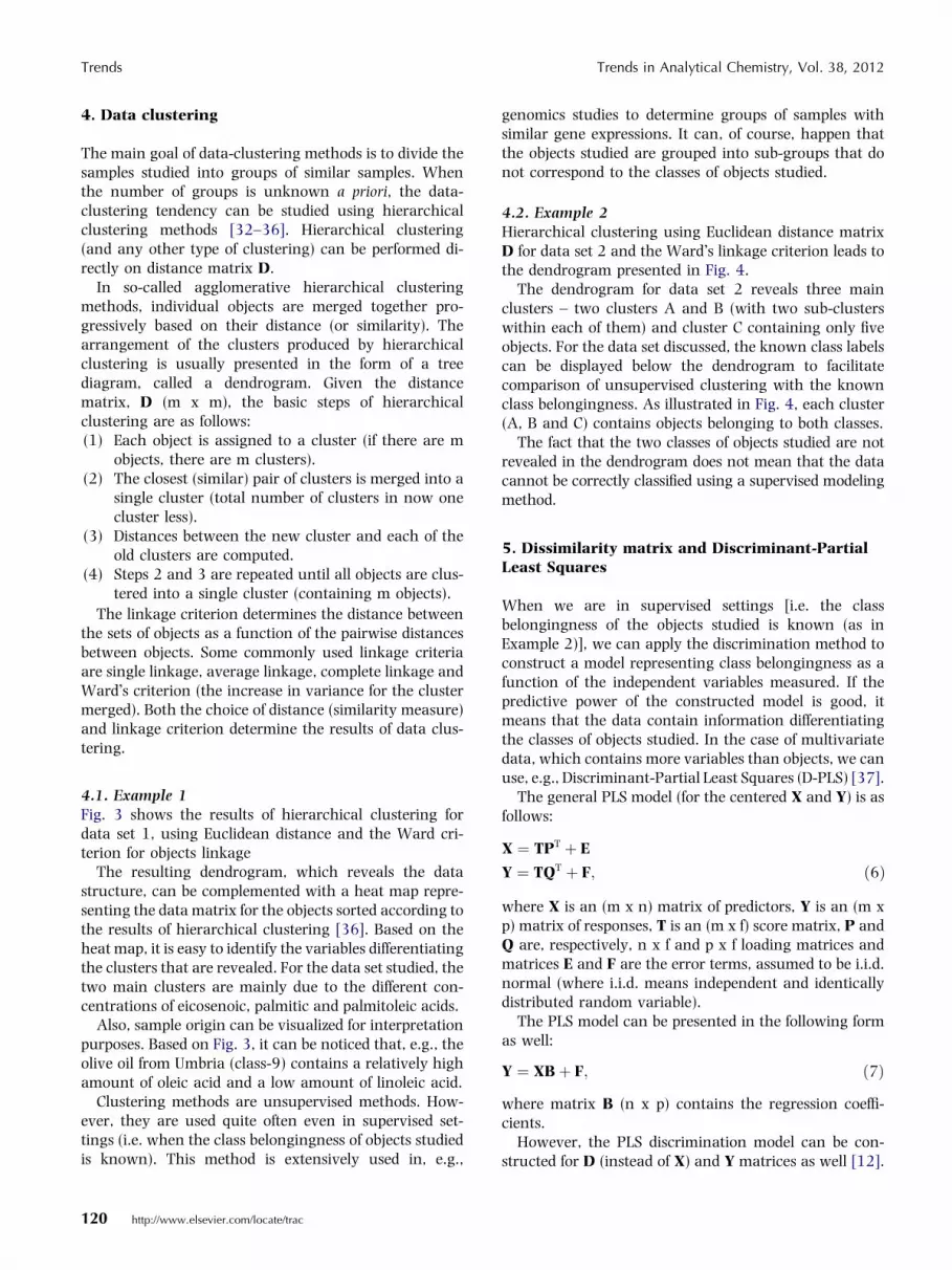
the sets of objects as a function of the pairwise distancesbetween objects. Some commonly used linkage criteriaare single linkage, average linkage, complete linkage andWard�s criterion (the increase in variance for the clustermerged). Both the choice of distance (similarity measure)and linkage criterion determine the results of data clus-tering.
4.1. Example 1Fig. 3 shows the results of hierarchical clustering fordata set 1, using Euclidean distance and the Ward cri-terion for objects linkage

The resulting dendrogram, which reveals the datastructure, can be complemented with a heat map repre-senting the data matrix for the objects sorted according tothe results of hierarchical clustering [36]. Based on theheat map, it is easy to identify the variables differentiatingthe clusters that are revealed. For the data set studied, thetwo main clusters are mainly due to the different con-centrations of eicosenoic, palmitic and palmitoleic acids.

Also, sample origin can be visualized for interpretationpurposes. Based on Fig. 3, it can be noticed that, e.g., theolive oil from Umbria (class-9) contains a relatively highamount of oleic acid and a low amount of linoleic acid.

Clustering methods are unsupervised methods. How-ever, they are used quite often even in supervised set-tings (i.e. when the class belongingness of objects studiedis known). This method is extensively used in, e.g.,


genomics studies to determine groups of samples withsimilar gene expressions. It can, of course, happen thatthe objects studied are grouped into sub-groups that donot correspond to the classes of objects studied.

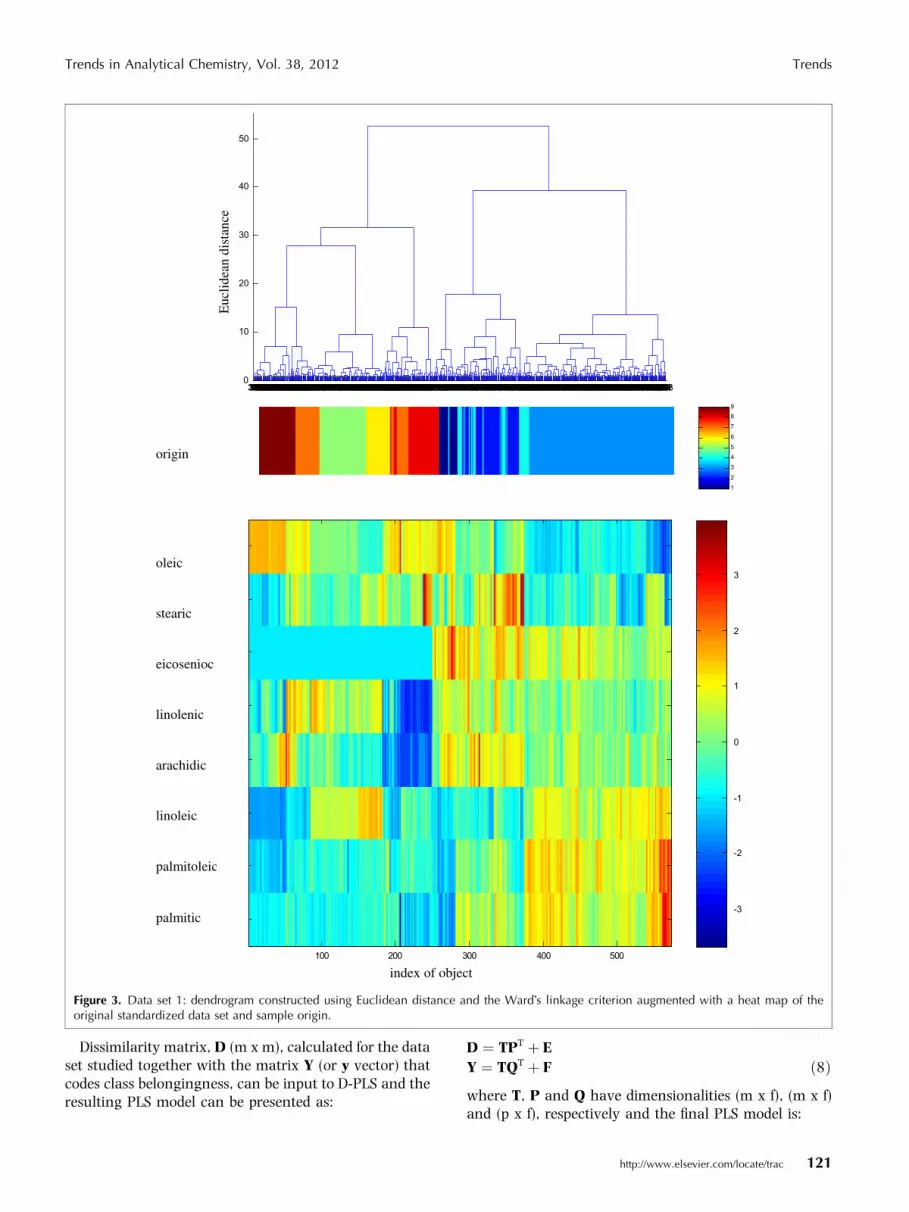
4.2. Example 2Hierarchical clustering using Euclidean distance matrixD for data set 2 and the Ward�s linkage criterion leads tothe dendrogram presented in Fig. 4.

The dendrogram for data set 2 reveals three mainclusters – two clusters A and B (with two sub-clusterswithin each of them) and cluster C containing only fiveobjects. For the data set discussed, the known class labelscan be displayed below the dendrogram to facilitatecomparison of unsupervised clustering with the knownclass belongingness. As illustrated in Fig. 4, each cluster(A, B and C) contains objects belonging to both classes.

The fact that the two classes of objects studied are notrevealed in the dendrogram does not mean that the datacannot be correctly classified using a supervised modelingmethod.

5. Dissimilarity matrix and Discriminant-PartialLeast Squares

When we are in supervised settings [i.e. the classbelongingness of the objects studied is known (as inExample 2)], we can apply the discrimination method toconstruct a model representing class belongingness as afunction of the independent variables measured. If thepredictive power of the constructed model is good, itmeans that the data contain information differentiatingthe classes of objects studied. In the case of multivariatedata, which contains more variables than objects, we canuse, e.g., Discriminant-Partial Least Squares (D-PLS) [37].

The general PLS model (for the centered X and Y) is asfollows:

X ¼ TPT þ E

Y ¼ TQT þ F; ð6Þ

where X is an (m x n) matrix of predictors, Y is an (m xp) matrix of responses, T is an (m x f) score matrix, P andQ are, respectively, n x f and p x f loading matrices andmatrices E and F are the error terms, assumed to be i.i.d.normal (where i.i.d. means independent and identicallydistributed random variable).

The PLS model can be presented in the following formas well:

Y ¼ XBþ F; ð7Þ

where matrix B (n x p) contains the regression coeffi-cients.

However, the PLS discrimination model can be con-structed for D (instead of X) and Y matrices as well [12].

123456789

345346330319327329321333339350338342320351352364365 9323349318328348344324326322340341325337347331335343332334336353367356359362355361363354358360357366 7227229236230220222244262228231234235221237243223232245256246226238263252261240264247233257242 5179124125127126186187173182140142157164166152160161174144156135143138163137162146148147159176128132141131134155153130149129181183136177180158151169170168133167150154139165145178184171175185172210208209 6197216192201205206213194204203188189215219211217200202191196218212190199214207193198195 8313248249250273280279286224265251259260266225239255253258254241267317268269285271290270289277311302283284315274291316303276292297275304300309310294295308278312272293298296282299281301287288305306307314 1 10 16 20 24 11 18 19 12 22 28 15 96 17 33 21 32 25 27 13 29 31 14 23 30101102117119118 2 34 68545512 37 76 40 47 75 4515 38113105518110111112 26 41 43 48 88 53 65 45 87 58122 81 85 86 35 74116 71 82 36 55 60 42 54 72 63 73 80 70 64 66 67 69 89542540 90 91 92106104107541424 39 50 51 78 79 77 84 46 56 62 49 59 52 83 57 61 44123 98114115 99103121100 93 97 94 95120 34224303683703691085025035095215085135195143725055045245265305335394284324364414664805313784215355374464584673994494685515653804774823814314344995275345601095105063914514234274034354604724743774024084184264334394445695705505573715075285384563765115435534205234945224174785005324965474975013754644704734064374384713874764985294294954505204864885254924815165174474594634653793973883904123844015363825544195525463924144554694055723834913894543864573954005445593853964154044113934133943984104074164093734524614904424454934874753744434624484535584254404794844834854895555635675485565665495645715615625680

10

20

30

40

50

oleic

stearic

eicosenioc

linolenic

arachidic

linoleic

palmitoleic

palmitic

origin

100 200 300 400 500

1

2

3

4

5

6

7

8-3

-2

-1

0

1

2

3

Euc

lidea

n di

stan

ce

index of object

Figure 3. Data set 1: dendrogram constructed using Euclidean distance and the Ward�s linkage criterion augmented with a heat map of theoriginal standardized data set and sample origin.


Dissimilarity matrix, D (m x m), calculated for the dataset studied together with the matrix Y (or y vector) thatcodes class belongingness, can be input to D-PLS and theresulting PLS model can be presented as:

D ¼ TPT þ E

Y ¼ TQT þ F ð8Þ

where T, P and Q have dimensionalities (m x f), (m x f)and (p x f), respectively and the final PLS model is:


0 10 20 30 40 50 60 70 80 90-1.5

-1

-0.5

0

0.5

1

1.5

index of objects

y pr

edic

ted

model set

0 10 20 30 40 50-1.5

-1

-0.5

0

0.5

1

1.5

index of objects

y pr

edic

ted

test set

Figure 5. Data set 2: Predicted class belongingness for a) model and b) independent test set.

18 62 6 19 60 61 64 94 75 85 95 70 71 97100 74 90 40 84 72 78 82 80 81 5 7 23 9 26 42 30 8 46 39 43 47 10 28 27 24 20 21 22 44 49 88 89 91 1 31 3 4 11 2 17 50 36 38 41 12 48 45 16 33 25 32 34 29 13 14 15 66 67 35 83 37 68 73 79 76 87 86 51 52 59 58 92 96 53 55 56 57 99 65 93 98 77 63 69 54

100

200

300

400

500

600

0 10 20 30 40 50 60 70 80 90 1000

0.1

0.2

0.3

0.4

0.5

0.6

0.7

0.8

0.9

1

A C B

Euc

lidea

n di

stan

ce

clusters

Figure 4. Data set 2: Dendrogram constructed based on Euclidean distance and the Ward�s linkage criterion.


Y ¼ DBþ F ð9Þ

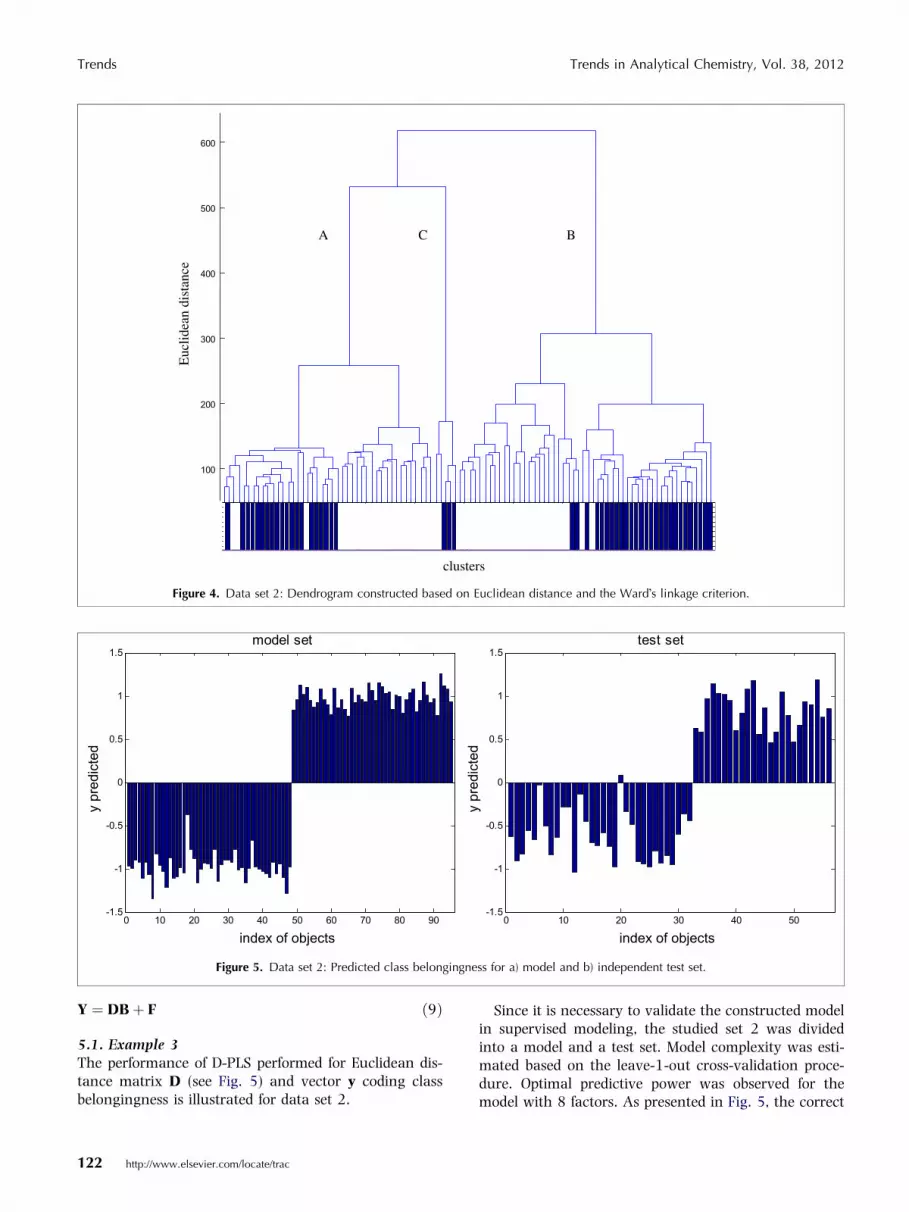
5.1. Example 3The performance of D-PLS performed for Euclidean dis-tance matrix D (see Fig. 5) and vector y coding classbelongingness is illustrated for data set 2.


Since it is necessary to validate the constructed modelin supervised modeling, the studied set 2 was dividedinto a model and a test set. Model complexity was esti-mated based on the leave-1-out cross-validation proce-dure. Optimal predictive power was observed for themodel with 8 factors. As presented in Fig. 5, the correct

0 100 200 300 400 500 600 700 800-1.5

-1

-0.5

0

0.5

1

1.5

index of objects

y pr

edic

ted

model set

0 100 200 300 400 500 600 700 800-1.5

-1

-0.5

0

0.5

1

1.5

index of objects

y pr

edic

ted

test set(a) (b)

Figure 6. Data set 3: Dissimilarity-PLS with 7 factors; y predicted for a) model and b) test set.


3000 3200 3400 3600 3800 4000 4200 4400 4600 4800 50000.4

0.5

0.6

0.7

0.8

0.9

1

1.1

1.2

1.3

1.4

3000 3200 3400 3600 3800 4000 4200 4400 4600 4800 50000.2

0.4

0.6

0.8

1

1.2

1.4

1.6

3000 3200 3400 3600 3800 4000 4200 4400 4600 4800 50000.2

0.4

0.6

0.8

1

1.2

1.4

1.6

3000 3200 3400 3600 3800 4000 4200 4400 4600 4800 50000.4

0.5

0.6

0.7

0.8

0.9

1

1.1

1.2

1.3

3000 3200 3400 3600 3800 4000 4200 4400 4600 4800 50000.4

0.5

0.6

0.7

0.8

0.9

1

1.1

1.2

1.3

3000 3200 3400 3600 3800 4000 4200 4400 4600 4800 50000.4

0.5

0.6

0.7

0.8

0.9

1

1.1

1.2

1.3

(d) (e) (f)

(a) (b) (c)

time time time

time time time

y y y

y y y

Figure 7. Noise-free MG data set: y test (blue) and y test predicted (red) based on PLS model for D and y with three different prediction horizons:a) 1; b) 5 and c) 10. Noisy (10%) MG data set: y test (blue) and y test predicted (red) based on PLS model for D and y with three different pre-diction horizons: d) 1; e) 5; and, f) 10.

classification rates for the model and test set are 100%and 98.21%, respectively.

The fact that it is possible to construct a discriminantmodel with good predictive power for the discussed data

set is quite surprising, taking into account the facts thatthe data contain 5 outlying objects in X-space (see Fig. 3,sub-group C) and that only a small fraction of genesdifferentiate the classes studied (i.e. there are many


(b)

class 1

class 2

class 1 class 2

(a)

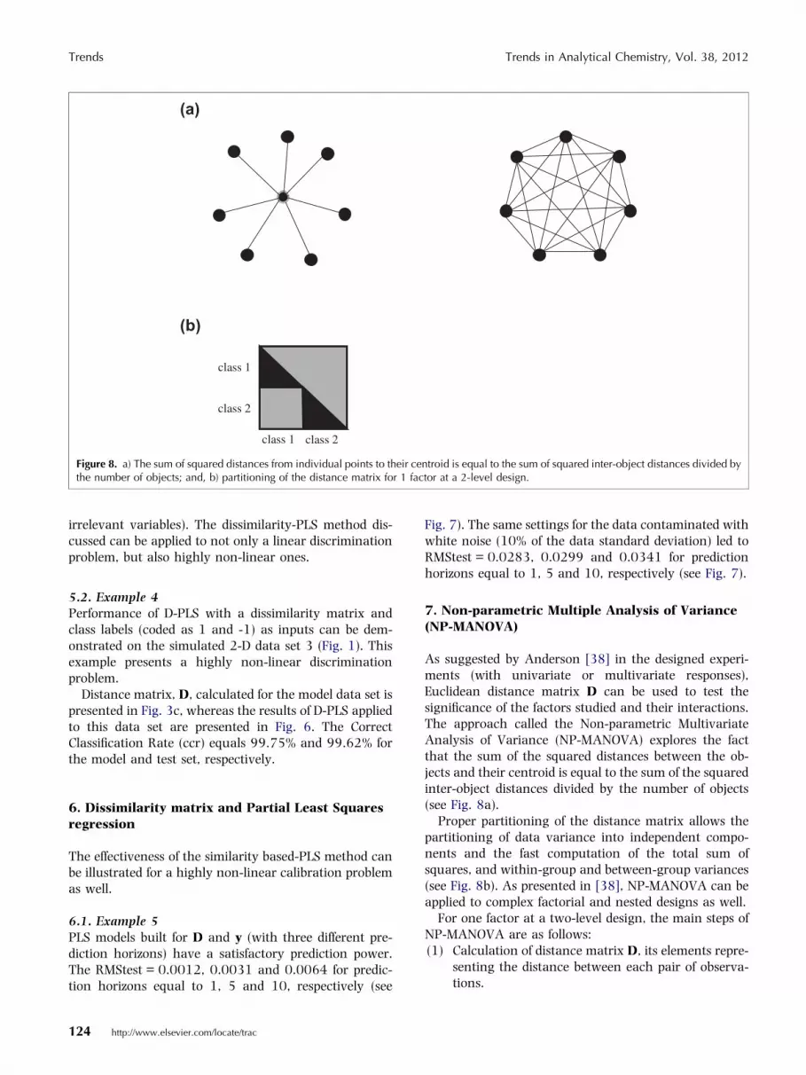
Figure 8. a) The sum of squared distances from individual points to their centroid is equal to the sum of squared inter-object distances divided bythe number of objects; and, b) partitioning of the distance matrix for 1 factor at a 2-level design.


irrelevant variables). The dissimilarity-PLS method dis-cussed can be applied to not only a linear discriminationproblem, but also highly non-linear ones.

5.2. Example 4Performance of D-PLS with a dissimilarity matrix andclass labels (coded as 1 and -1) as inputs can be dem-onstrated on the simulated 2-D data set 3 (Fig. 1). Thisexample presents a highly non-linear discriminationproblem.

Distance matrix, D, calculated for the model data set ispresented in Fig. 3c, whereas the results of D-PLS appliedto this data set are presented in Fig. 6. The CorrectClassification Rate (ccr) equals 99.75% and 99.62% forthe model and test set, respectively.

6. Dissimilarity matrix and Partial Least Squaresregression

The effectiveness of the similarity based-PLS method canbe illustrated for a highly non-linear calibration problemas well.

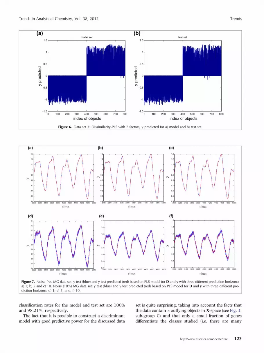
6.1. Example 5PLS models built for D and y (with three different pre-diction horizons) have a satisfactory prediction power.The RMStest = 0.0012, 0.0031 and 0.0064 for predic-tion horizons equal to 1, 5 and 10, respectively (see


Fig. 7). The same settings for the data contaminated withwhite noise (10% of the data standard deviation) led toRMStest = 0.0283, 0.0299 and 0.0341 for predictionhorizons equal to 1, 5 and 10, respectively (see Fig. 7).

7. Non-parametric Multiple Analysis of Variance(NP-MANOVA)

As suggested by Anderson [38] in the designed experi-ments (with univariate or multivariate responses),Euclidean distance matrix D can be used to test thesignificance of the factors studied and their interactions.The approach called the Non-parametric MultivariateAnalysis of Variance (NP-MANOVA) explores the factthat the sum of the squared distances between the ob-jects and their centroid is equal to the sum of the squaredinter-object distances divided by the number of objects(see Fig. 8a).

Proper partitioning of the distance matrix allows thepartitioning of data variance into independent compo-nents and the fast computation of the total sum ofsquares, and within-group and between-group variances(see Fig. 8b). As presented in [38], NP-MANOVA can beapplied to complex factorial and nested designs as well.

For one factor at a two-level design, the main steps ofNP-MANOVA are as follows:(1) Calculation of distance matrix D, its elements repre-

senting the distance between each pair of observa-tions.

(a) (c)

(b) (d)

10 20 30 40 50 60 70 80 90 100

10

20

30

40

50

60

70

80

90

100

20 40 60 80 100

10

20

30

40

50

60

70

80

90

100

50

100

150

200

250

0 10 20 30 40 50 60 70 80 90 1000

0.5

1

1.5

2

2.5 x 104

0 1 2 3 4 5 60

100

200

300

400

500

600

class 1 class 2

F

clas

s 2

clas

s 1

index of objectindex of object

inde

x of

obj

ect

inde

x of

obj

ect

index of object

Euc

lidea

n m

ean

dis

tanc

e

Figure 9. a) Matrix containing squared distances calculated for gene expression data set 2 (balanced model set of the dimensionality 100 x22415); b) histogram of null hypothesis with marked F – observed value; c) Euclidean distance matrix for data set 2; and, d) mean distance plotfor X-outliers identification for data set 2.


(2) Calculation of the total sum of squares:

SST ¼1

m

Xm�1

i¼1

Xm

j¼iþ1d2

ij ð10Þ

where m denotes the total number of observations anddij represents ij-th element of matrix D.(3) Calculation of the within-group variance:

SSW ¼1

n

Xm�1

i¼1

Xm

j¼iþ1dijeij ð11Þ

where n is the number of observation per group and eij

takes the value 1, if observations i and j belong to thesame group, otherwise it takes the value of zero.

Then SSA ¼ SST � SSW ð12Þ

(4) Calculation of the pseudo F-ratio:

SS =ða� 1Þ
F ¼ A
SSW=ðm� aÞ ð13Þ

where a denotes the number of groups.(5) Permutation (randomization) test and calculation of

the p-value:

ðNo: of Fp � FÞ
p ¼
Total no: of Fp ð14Þ

To estimate the entire distribution of the pseudoF-statistics under a true null hypothesis for the data setstudied, it is necessary to perform a permutation (ran-domization) test [38–40], [i.e. to repeat the randomshuffling of the labels of the D matrix and recalculate anew value of the Fp-statistics (index p denotes permu-tations) many times]. The F value observed for the


0 10 20 30 40 50 60 70 80 90 1000

0.5

1

1.5

2

2.5 x 104

0 10 20 30 40 50 60 70 80 90 1000

1000

2000

3000

4000

5000

6000

7000

8000

9000

10000

0 10 20 30 40 50 60 70 80 90 1000

20

40

60

80

100

120

140

160

180

200

Euclidean Manhattan Rank transformed data

(a) (b) (c)

index of object index of object index of object

mea

n di

stan

ce

mea

n di

stan

ce

mea

n di

stan

ce

Figure 10. Mean distance plots for a) Euclidean distance; b) Manhattan distance; and, c) Euclidean distance of the rank transformed data set 2.


experimental data can then be compared with the dis-tribution of the Fp-values for a true null hypothesis andthe p-value calculated according to Equation (14) iscompared with an a priori selected significance level. Inour study, a was set to 0.01 and 10,000 permutationswere performed.

It should be pointed out that, in the permutation testdescribed above, the distance matrix is calculated onlyonce and only the labels of objects are shuffled. Thus, thecalculation time of the permutation test is a 100 timesless than that of a permutation test performed using theASCA approach [41].

The attractiveness of NP-MANOVA is also because thismethod can be applied to any type of distance (or dis-similarity) measure. If the data-exploration step suggeststhat data may be contaminated with outlying objects,variables or elements, the classical approach should bereplaced by the robust version of NP-MANOVA [42,43].One of the simplest methods is to rank transform (RT)the analyzed data set [38,44,45]. All further steps ofNP-MANOVA are identical with those described earlier.

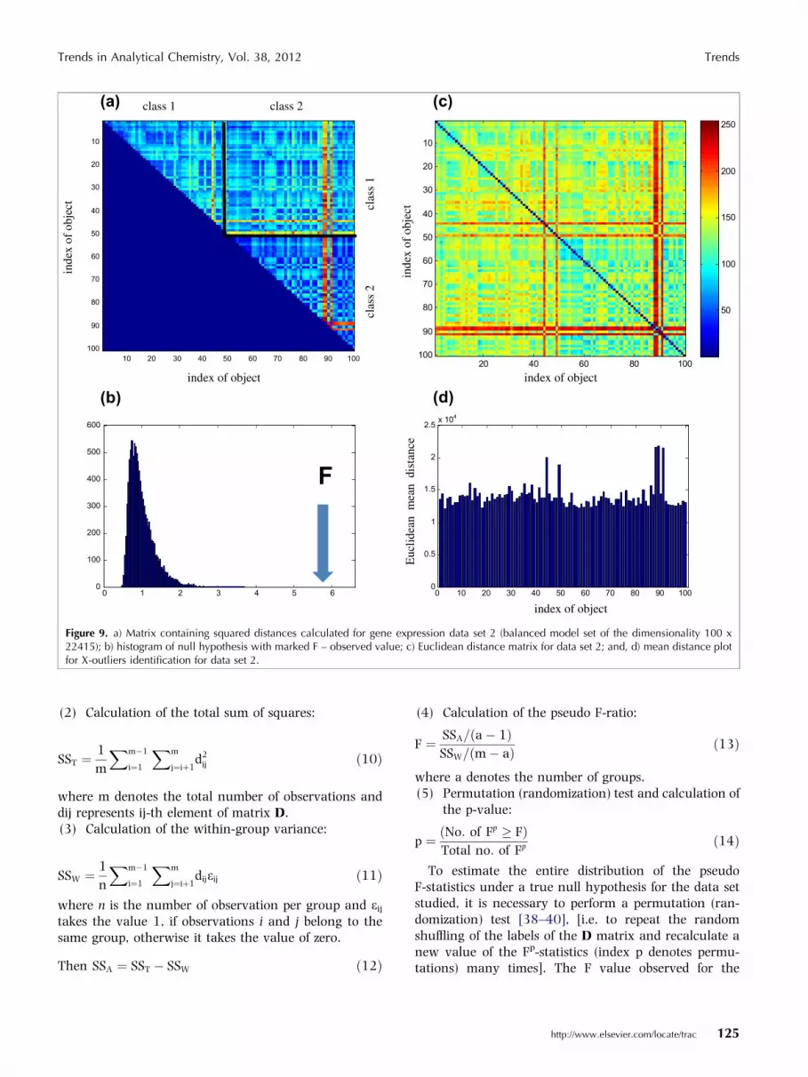
The performance of NP-MANOVA is demonstrated fordata set 2 (gene-expression data). The squared elementsof the upper part of a distance matrix built for the modelset are used to calculate the total variance and within-groups variance and then the pseudo F-ratio(F = 5.804). The observed F value is compared with thedistribution of the Fp values for a true null hypothesis(see Fig. 9) and this comparison allows the conclusion tobe drawn that the difference between two classes of ob-jects studied is statistically significant (p = 0.000).

8. X-outliers detection

When working with dissimilarity matrices, it is very easyto identify X-outliers (i.e. objects that are far away fromthe data majority in the X-space). This can be done basedon the mean distance of a given object to the remainingones. For illustrative purposes, Figs. 9c and 9d show the


Euclidean distance matrix together with the �mean dis-tance plot�, calculated for data set 2.

As you can see, objects 73, 79, 139, 140 and 142 areoutlying in the X-space. Of course, X-outliers (leverages)are not necessarily the outliers in the classificationmodel; however, their presence suggests that, if theclassification model does not have the desired perfor-mance, the outlier-sensitive Euclidean distance should bereplaced with a more robust dissimilarity measure (e.g.,Manhattan distance).

A mean distance plot can also be used at the stage ofthe classification of new samples (or regression). If thenew samples are outside the model range (i.e. if they arefar from the objects belonging to the model set), modelprediction will be doubtful.

9. Robust dissimilarity measures

In the case of contaminated data (i.e. the data withoutliers in the X-space), the previously discussedEuclidean distance should be replaced with a morerobust dissimilarity measure (e.g., the Manhattan dis-tance). As an alternative approach, the rank transformof the data studied, followed by the calculation of theEuclidean distance can be proposed. Rank transformsimply refers to replacing the elements of the givenvariable with its ranks. This means that all elements ofthe i-th variable are ranked from the smallest to thelargest, with the smallest observation having rank 1, thesecond smallest rank 2, etc.

An example of the application of a robust dissimilaritymeasure to studying the effect of the potato-droughttolerance based on a proteomic study is available [45].

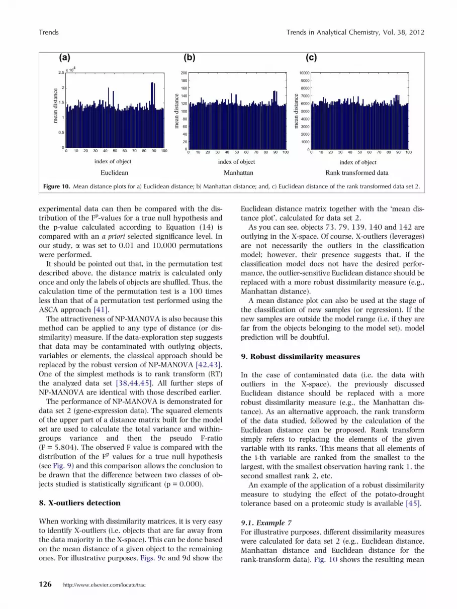
9.1. Example 7For illustrative purposes, different dissimilarity measureswere calculated for data set 2 (e.g., Euclidean distance,Manhattan distance and Euclidean distance for therank-transform data). Fig. 10 shows the resulting mean

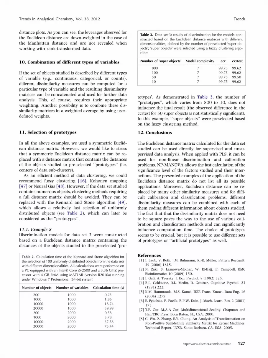
Table 3. Data set 3: results of discrimination for the models con-structed based on the Euclidean distance matrices with differentdimensionalities, defined by the number of preselected �super ob-jects�; �super objects� were selected using a fuzzy clustering algo-


distance plots. As you can see, the leverages observed forthe Euclidean distance are down-weighted in the case ofthe Manhattan distance and are not revealed whenworking with rank-transformed data.

rithm

Number of �super objects� Model complexity ccr ccrtest

800 7 99.75 99.62100 7 99.75 99.6250 7 99.75 99.5010 7 99.75 99.62

10. Combination of different types of variables

If the set of objects studied is described by different typesof variable (e.g., continuous, categorical, or counts),different dissimilarity measures can be computed for aparticular type of variable and the resulting dissimilaritymatrices can be concatenated and used for further dataanalysis. This, of course, requires their appropriateweighting. Another possibility is to combine these dis-similarity matrices in a weighted average by using user-defined weights.

11. Selection of prototypes

In all the above examples, we used a symmetric Euclid-ean distance matrix. However, we would like to stressthat a symmetric Euclidean distance matrix can be re-placed with a distance matrix that contains the distancesof the objects studied to pre-selected ‘‘prototypes’’ (i.e.centers of data sub-clusters).

As an efficient method of data clustering, we couldrecommend fuzzy clustering [46], Kohonen mapping[47] or Neural Gas [48]. However, if the data set studiedcontains numerous objects, clustering methods requiringa full distance matrix should be avoided. They can bereplaced with the Kennard and Stone algorithm [49],which allows a relatively fast selection of uniformlydistributed objects (see Table 2), which can later beconsidered as the ‘‘prototypes’’.

11.1. Example 8Discrimination models for data set 3 were constructedbased on a Euclidean distance matrix containing thedistances of the objects studied to the preselected �pro-

Table 2. Calculation time of the Kennard and Stone algorithm forthe selection of 100 uniformly distributed objects from the data setswith different dimensionalities. All calculations were performed ona PC equipped with an Intel� Core i5-2500 and a 3.36 GHZ pro-cessor with 4 GB RAM using MATLAB (version R2010a) runningunder Windows 7 Professional (64-bit system)

Number of objects Number of variables Calculation time (s)

200 1000 0.251000 1000 1.8610000 1000 18.7420000 1000 39.99200 2000 0.581000 2000 3.7810000 2000 37.5820000 2000 75.44

totypes�. As demonstrated in Table 3, the number of‘‘prototypes’’, which varies from 800 to 10, does notinfluence the final result (the observed difference in theccrtest for 50 super objects is not statistically significant).In this example, ‘‘super objects’’ were preselected basedon the fuzzy clustering method.

12. Conclusions

The Euclidean distance matrix calculated for the data setstudied can be used directly for supervised and unsu-pervised data analysis. When applied with PLS, it can beused for non-linear discrimination and calibrationproblems. NP-MANOVA allows the fast calculation of thesignificance level of the factors studied and their inter-actions. The presented examples of the application of theEuclidean distance matrix do not list all its possibleapplications. Moreover, Euclidean distance can be re-placed by many other similarity measures and for diffi-cult calibration and classification problems, differentdissimilarity measures can be combined with each ofthem coding different information about objects studied.The fact that that the dissimilarity matrix does not needto be square paves the way to the use of various cali-bration and classification methods and can significantlyinfluence computation time. The choice of prototypesseems to be crucial, but it is possible to use different setsof prototypes or ‘‘artificial prototypes’’ as well.

References[1] J. Laub, V. Roth, J.M. Buhmann, K.-R. Muller, Pattern Recognit.

39 (2006) 1815.

[2] N. Zaki, S. Lazarova-Molnar, W. El-Hajj, P. Campbell, BMC

Bioinformatics 10 (2009) 150.

[3] I. Gati, A. Tversky, J. Exp. Psychol. 8 (1982) 325.

[4] R.L. Goldstone, D.L. Medin, D. Gentner, Cognitive Psychol. 23

(1991) 222.

[5] K.M. Hammouda, M.S. Kamel, IEEE Trans. Knowl. Data Eng. 16

(2004) 1279.

[6] E. Pekalska, P. Paclık, R.P.W. Duin, J. Mach. Learn. Res. 2 (2001)

175.

[7] T.F. Cox, M.A.A Cox, Multidimensional Scaling, Chapman and

Hall/CRC Press, Boca Raton, FL, USA, 2000.

[8] G. Wu, Z. Zhang, E.Y. Chang. An Analysis of Transformation on

Non-Positive Semidefinite Similarity Matrix for Kernel Machines,

Technical Report, UCSB, Santa Barbara, CA, USA, 2005.



[9] B. Scholkopf, R. Herbrich, A.J. Smola, Lecture Notes Comput. Sci.

2111 (2001) 416.

[10] W. Duch, Control Cybernet. 29 (2000) 937.

[11] H.-T. Lin, C.-J. Lin, A Study on Sigmoid Kernel for SVM and the

Training of Non-PSD Kernels by SMO-Type Methods, Department

of Computer Science and Information Engineering, National

Taiwan University, Taiwan, 2003.

[12] P. Zerzucha, M. Daszykowski, B. Walczak, Chemom. Intell. Lab.

Syst. 110 (2012) 156.

[13] B. Walczak, W. Wegscheider, Anal. Chim. Acta 283 (1993) 508.

[14] G.P. Zhang, B.E. Patuwo, M.Y. Hu, Comput. Oper. Res. 28 (2001)

381.

[15] S. Mukherjee, E. Osuna, F. Girosi. Non-linear prediction of chaotic

time series using a support vector machine, in: J. Principe, L. Gile,

N. Morgan, E. Wilson (Editors), Neural Networks for Signal

Processing VII — Proc. 1997 IEEE Workshop, IEEE, New York,

USA, 1997.

[16] S. Abe, Support Vector Machines for Pattern Classification,

Springer-Verlag, New York, USA, 2005.

[17] B. Scholkopf, A.J. Smola, Learning with Kernels: Support Vector

Machines, Optimization, MIT Press, Cambridge, MA, USA, Reg-

ularization, 2001.

[18] B. Walczak, D.L. Massart, Anal. Chim. Acta 331 (1996) 177.

[19] B. Walczak, D.L. Massart, Anal. Chim. Acta 331 (1996) 187.

[20] T. Czekaj, W. Wu, B. Walczak, J. Chemom. 19 (2005) 341.

[21] B.M. Nicolai, K.I. Theron, J. Lammertyn, Chemom. Intell. Lab.

Syst. 85 (2007) 243.

[22] J. Mercer, Philos. Trans. Roy. Soc. London A 209 (1909) 415.

[23] E. Pekalska, P. Paclık, R.P.W. Duin, J. Machine, Learn. Res. 2

(2001) 175.

[24] J. Shawe-Taylor, N. Cristianini, Kernel Methods for Pattern

Analysis, Cambridge University Press, Cambridge, UK, 2004.

[25] B.R. Sarker, K.M. Saiful Islam, Computers and Industrial Engi-

neering 37 (1999) 769.

[26] B. Scholkopf, The kernel trick for distances, in: Advances in

Neural Information Processing Systems 13, Proc. Fourteenth

Annual Neural Info. Process. Syst. Conf. (NIPS 2000), MIT Press,

Cambridge, MA, USA.

[27] M. Forina, C. Armanino, Annal. Chim. 72 (1987) 127.

[28] http://genome-www5stanford.edu/cgi-bin/publication/viewPubli-

cation.pl?pub_no=107 [29 September 2004].

[29] T. Czekaj, W. Wu, B. Walczak, Talanta 76 (2008) 564.


[30] M.C. Mackey, L. Glass, Science (Washington, DC) 197 (1977)

287.

[31] Mackey-Glass time series generator (www.mathworks.com/mat-

labcentral/fileexchange/24390-mackey-glass-time-series-genera-

tor/content/html/mackeyglass.html).

[32] D.L. Massart, L. Kaufman, The Interpretation of Analytical Data

by the Use of Cluster Analysis, Wiley, New York, USA, 1983.

[33] W. Vogt, D. Nagel, H. Sator, Cluster Analysis in Clinical

Chemistry; A Model, Wiley, New York, USA, 1987.

[34] L. Kaufman, P.J. Rousseeuw, Finding Groups in Data; An

Introduction to Cluster Analysis, Wiley, New York, USA, 1990.

[35] H.C. Romesburg, Cluster Analysis for Researchers, Lifetime

Learning Publications, Belmont, CA, USA, 1984.

[36] A. Smolinski, B. Walczak, J.W. Einax, Chemom. Intell. Lab. Syst.

64 (2002) 45.

[37] R. Sabatier, M. Vivein, P. Amenta, Two Approaches for Discrim-

inant Partial Least Square, in: M. Schader, W. Gaul, M. Vichi

(Editors), Between Data Science and Applied Data Analysis,

Springer-Verlag, Berlin, Germany, 2003.

[38] M.J. Anderson, Aust. Ecol. 26 (2001) 32.

[39] M.J. Anderson, Can. J. Fish. Aquat. Sci. 58 (2001) 626.

[40] M.J. Anderson, C.J.F. ter Braak, J. Stat. Comput. Simul. 73 (2003)

85.

[41] A.K. Smilde, J.J. Jansen, H.C.J. Hoefsloot, J. Van der Greef, M.E.

Timmerman, Bioinformatics 21 (2005) 3043.

[42] J.J. Jansen, H.C.J. Hoefsloot, J. Van der Greef, M.E. Timmerman,

J.A. Westerhuis, A.K. Smilde, J. Chemom. 19 (2005) 469.

[43] D.J. Vis, J.A. Westerhuis, A.K. Smilde, J. van der Greef, BMC

Bioinform. 8 (2007) 322.

[44] J.R. de Haan, S. Bauerschmidt, R.C. van Schaik, E. Piek, L.M.C.

Buydens, R. Wehrens, Chemom. Intell. Lab. Syst. 98 (2009) 38.

[45] P. Zerzucha, D. Boguszewska, B. Zagdanska, B. Walczak, Anal.

Chim. Acta 717 (2012) 1.

[46] M. Ankrest, M. Breunig, H. Kriegel, J. Sander, OPTICS: Ordering

Points to Identify the Clustering Structure (available from

www.dbs.informatik.uni-muenchen.de/cgi-bin/papers?query=-CO).

[47] J. Zupan, J. Gasteiger, Neural Networks in Chemistry and Drug

Design, 2nd Edition., Wiley-VCH, Weinheim, Germany, 1999.

[48] M. Daszykowski, B. Walczak, D.L. Massart, J. Chem. Inf. Comput.

Sci. 42 (2002) 1378.

[49] R.W. Kennard, L.A. Stone, Technometrics 11 (1969) 137.

http://genome-www5stanford.edu/cgi-bin/publication/viewPublication.pl?pub_no=107

http://genome-www5stanford.edu/cgi-bin/publication/viewPublication.pl?pub_no=107

http://www.mathworks.com/matlabcentral/fileexchange/24390-mackey-glass-time-series-generator/content/html/mackeyglass.html



http://www.dbs.informatik.uni-muenchen.de/cgi-bin/papers?query=-CO

concept of (dis)similarity in data analysis

Documents