Logisti Regression Rollin Brant 2007

Contents3 Logisti Regression 23.1 The Logisti Curve . . . . . . . . . . . . . . . . . . . . . . . . . . . . 33.2 Fitting a Logisti Curve . . . . . . . . . . . . . . . . . . . . . . . . . 53.3 Multiple Logisti Regression . . . . . . . . . . . . . . . . . . . . . . . 63.4 Mathemati al review: Odds and Logs . . . . . . . . . . . . . . . . . . 83.4.1 Odds and Odds Ratios . . . . . . . . . . . . . . . . . . . . . . 83.4.2 Odds and Logisti Regression . . . . . . . . . . . . . . . . . . 103.4.3 An example . . . . . . . . . . . . . . . . . . . . . . . . . . . . 103.5 Logisti regression: Inferen e . . . . . . . . . . . . . . . . . . . . . . . 123.5.1 Sampling behaviour of the m.l.e.'s . . . . . . . . . . . . . . . . 123.5.2 Multi-parameter inferen es . . . . . . . . . . . . . . . . . . . . 153.6 Examining the Fit of the Logisti Model . . . . . . . . . . . . . . . . 163.6.1 Predi ted values . . . . . . . . . . . . . . . . . . . . . . . . . . 163.6.2 Predi tive strength of the �t . . . . . . . . . . . . . . . . . . . 183.6.3 Generalized residuals: Observed - Expe ted proportions . . . . 193.6.4 Goodness of Fit . . . . . . . . . . . . . . . . . . . . . . . . . . 203.7 Sampling Design and the Logisti Regression Model . . . . . . . . . . 213.8 Ordinal Logisti Regression . . . . . . . . . . . . . . . . . . . . . . . 21

1

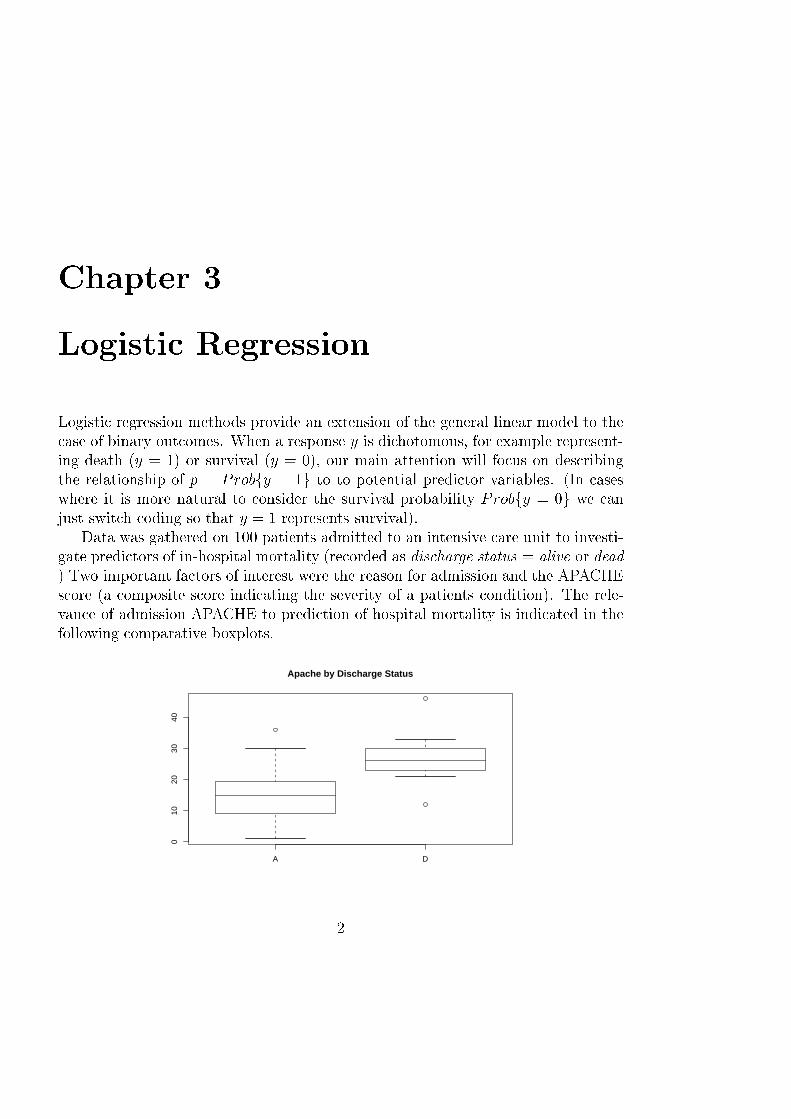
Chapter 3Logisti RegressionLogisti regression methods provide an extension of the general linear model to the ase of binary out omes. When a response y is di hotomous, for example represent-ing death (y = 1) or survival (y = 0), our main attention will fo us on des ribingthe relationship of p = Probfy = 1g to to potential predi tor variables. (In aseswhere it is more natural to onsider the survival probability Probfy = 0g we anjust swit h oding so that y = 1 represents survival).Data was gathered on 100 patients admitted to an intensive are unit to investi-gate predi tors of in-hospital mortality (re orded as dis harge status = alive or dead) Two important fa tors of interest were the reason for admission and the APACHEs ore (a omposite s ore indi ating the severity of a patients ondition). The rele-van e of admission APACHE to predi tion of hospital mortality is indi ated in thefollowing omparative boxplots.

A D

010

2030

40

Apache by Discharge Status

2

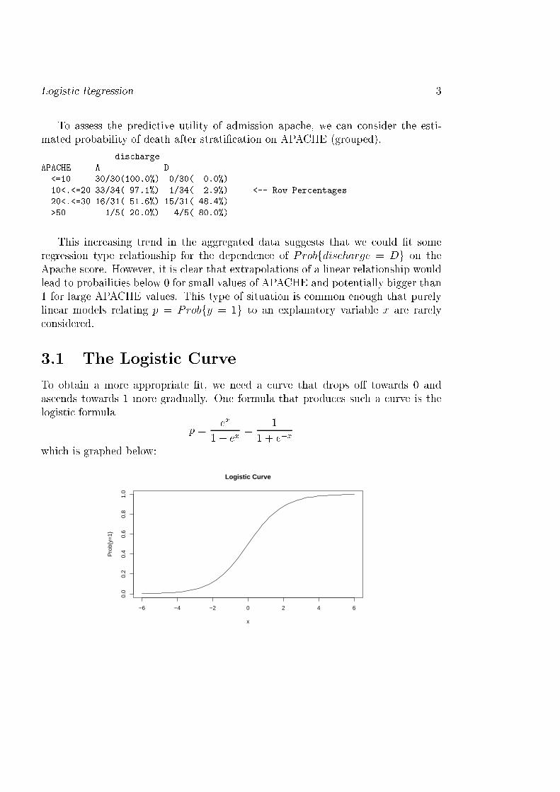
Logisti Regression 3To assess the predi tive utility of admission apa he, we an onsider the esti-mated probability of death after strati� ation on APACHE (grouped).dis hargeAPACHE A D<=10 30/30(100.0%) 0/30( 0.0%)10<.<=20 33/34( 97.1%) 1/34( 2.9%) <-- Row Per entages20<.<=30 16/31( 51.6%) 15/31( 48.4%)>50 1/5( 20.0%) 4/5( 80.0%)This in reasing trend in the aggregated data suggests that we ould �t someregression type relationship for the dependen e of Probfdis harge = Dg on theApa he s ore. However, it is lear that extrapolations of a linear relationship wouldlead to probailities below 0 for small values of APACHE and potentially bigger than1 for large APACHE values. This type of situation is ommon enough that purelylinear models relating p = Probfy = 1g to an explanatory variable x are rarely onsidered.3.1 The Logisti CurveTo obtain a more appropriate �t, we need a urve that drops o� towards 0 andas ends towards 1 more gradually. One formula that produ es su h a urve is thelogisti formula p = ex1 + ex = 11 + e�xwhi h is graphed below:

−6 −4 −2 0 2 4 6

0.0

0.2

0.4

0.6

0.8

1.0

Logistic Curve

x

Pro

b{y=

1}

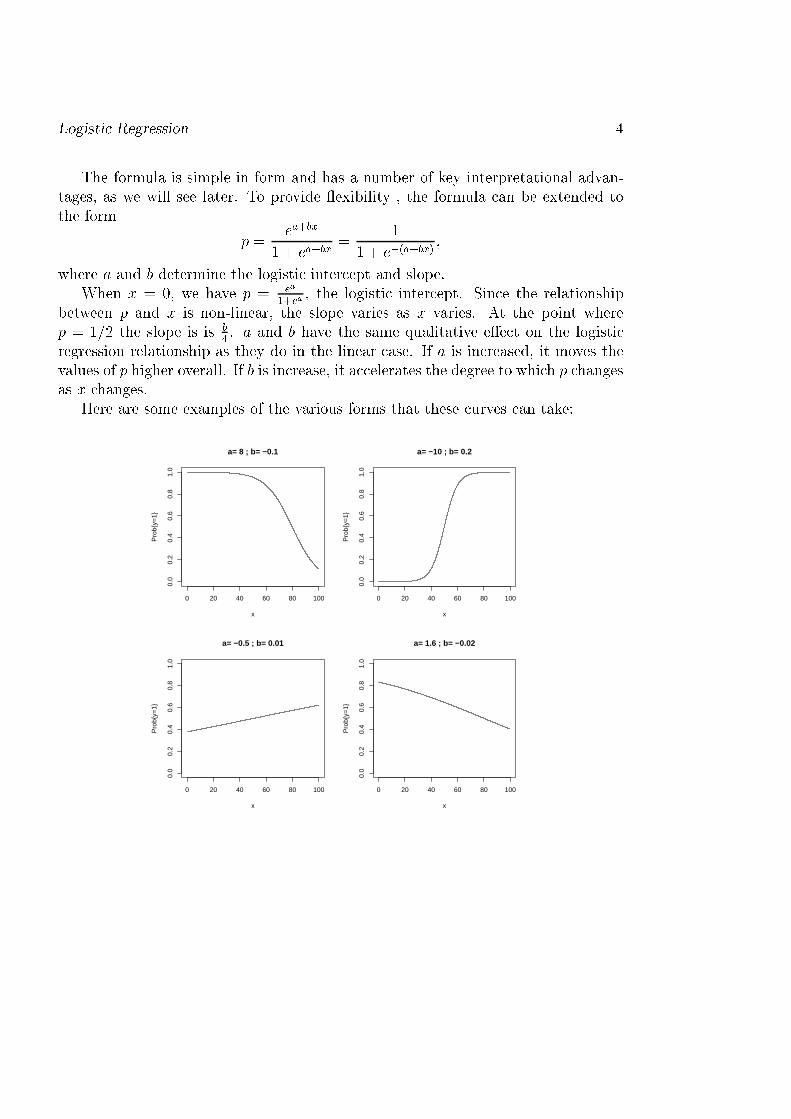
Logisti Regression 4The formula is simple in form and has a number of key interpretational advan-tages, as we will see later. To provide exibility , the formula an be extended tothe form p = ea+bx1 + ea+bx = 11 + e�(a+bx) ;where a and b determine the logisti inter ept and slope.When x = 0, we have p = ea1+ea , the logisti inter ept. Sin e the relationshipbetween p and x is non-linear, the slope varies as x varies. At the point wherep = 1=2 the slope is is b4 . a and b have the same qualitative e�e t on the logisti regression relationship as they do in the linear ase. If a is in reased, it moves thevalues of p higher overall. If b is in rease, it a elerates the degree to whi h p hangesas x hanges.Here are some examples of the various forms that these urves an take:0 20 40 60 80 100

0.0

0.2

0.4

0.6

0.8

1.0

a= 8 ; b= −0.1

x

Pro

b{y=

1}

0 20 40 60 80 100

0.0

0.2

0.4

0.6

0.8

1.0

a= −10 ; b= 0.2

x

Pro

b{y=

1}

0 20 40 60 80 100

0.0

0.2

0.4

0.6

0.8

1.0

a= −0.5 ; b= 0.01

x

Pro

b{y=

1}

0 20 40 60 80 100

0.0

0.2

0.4

0.6

0.8

1.0

a= 1.6 ; b= −0.02

x

Pro

b{y=

1}

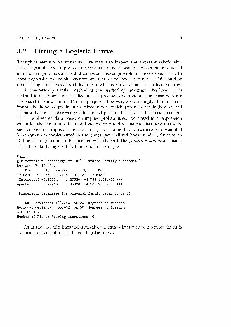
Logisti Regression 53.2 Fitting a Logisti CurveThough it seems a bit unnatural, we may also inspe t the apparent relationshipbetween p and x by simply plotting y versus x and hoosing the parti ular values ofa and b that produ es a line that omes as lose as possible to the observed data. Inlinear regression we use the least squares method to hoose estimates. This ould bedone for logisti urves as well, leading to what is known as non-linear least squares.A theoreti ally similar method is the method of maximum likelihood. Thismethod is des ribed and justi�ed in a supplementary handout for those who areinterested to known more. For our purposes, however, we an simply think of max-imum likelihood as produ ing a �tted model whi h produ es the highest overallprobability for the observed y-values of all possible �ts, i.e. is the most onsistentwith the observed data based on implied probabilities. No losed-form expressionexists for the maximum likelihood values for a and b. Instead, iterative methods,su h as Newton-Raphson must be employed. The method of iteratively re-weightedleast squares is implemented in the glm() (generallized linear model ) fun tion inR. Logisti regression an be spe i�ed with the with the family = binomial option,with the default logisti link fun tion. For exampleCall:glm(formula = (dis harge == "D") ~ apa he, family = binomial)Devian e Residuals:Min 1Q Median 3Q Max-2.0870 -0.4965 -0.2175 -0.1137 2.6182(Inter ept) -6.12034 1.27530 -4.799 1.59e-06 ***apa he 0.22716 0.05326 4.265 2.00e-05 ***---(Dispersion parameter for binomial family taken to be 1)Null devian e: 100.080 on 99 degrees of freedomResidual devian e: 65.482 on 98 degrees of freedomAIC: 69.482Number of Fisher S oring iterations: 6As in the ase of a linear relationship, the most dire t way to interpret the �t isby means of a graph of the �tted (logisti ) urve.

Logisti Regression 6

0 10 20 30 40

0.0

0.2

0.4

0.6

0.8

1.0

Logistic Fit

APACHE

Dis

char

ge =

D

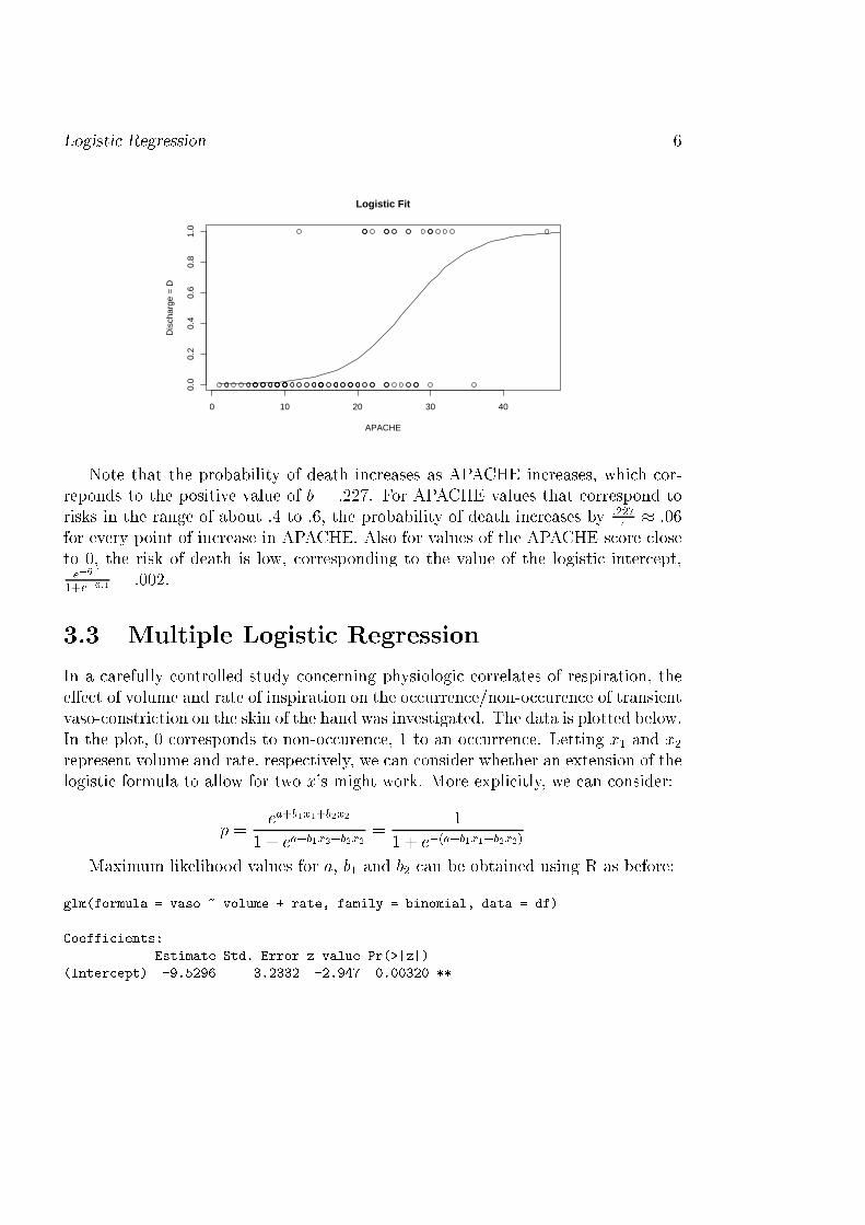
Note that the probability of death in reases as APACHE in reases, whi h or-reponds to the positive value of b = :227. For APACHE values that orrespond torisks in the range of about .4 to .6, the probability of death in reases by :2274 � :06for every point of in rease in APACHE. Also for values of the APACHE s ore loseto 0, the risk of death is low, orresponding to the value of the logisti inter ept,e�6:11+e�6:1 = :002.3.3 Multiple Logisti RegressionIn a arefully ontrolled study on erning physiologi orrelates of respiration, thee�e t of volume and rate of inspiration on the o urren e/non-o uren e of transientvaso- onstri tion on the skin of the hand was investigated. The data is plotted below.In the plot, 0 orresponds to non-o uren e, 1 to an o urren e. Letting x1 and x2represent volume and rate, respe tively, we an onsider whether an extension of thelogisti formula to allow for two x's might work. More expli itly, we an onsider:p = ea+b1x1+b2x21 + ea+b1x2+b2x2 = 11 + e�(a+b1x1+b2x2)Maximum likelihood values for a, b1 and b2 an be obtained using R as before:glm(formula = vaso ~ volume + rate, family = binomial, data = df)Coeffi ients:Estimate Std. Error z value Pr(>|z|)(Inter ept) -9.5296 3.2332 -2.947 0.00320 **

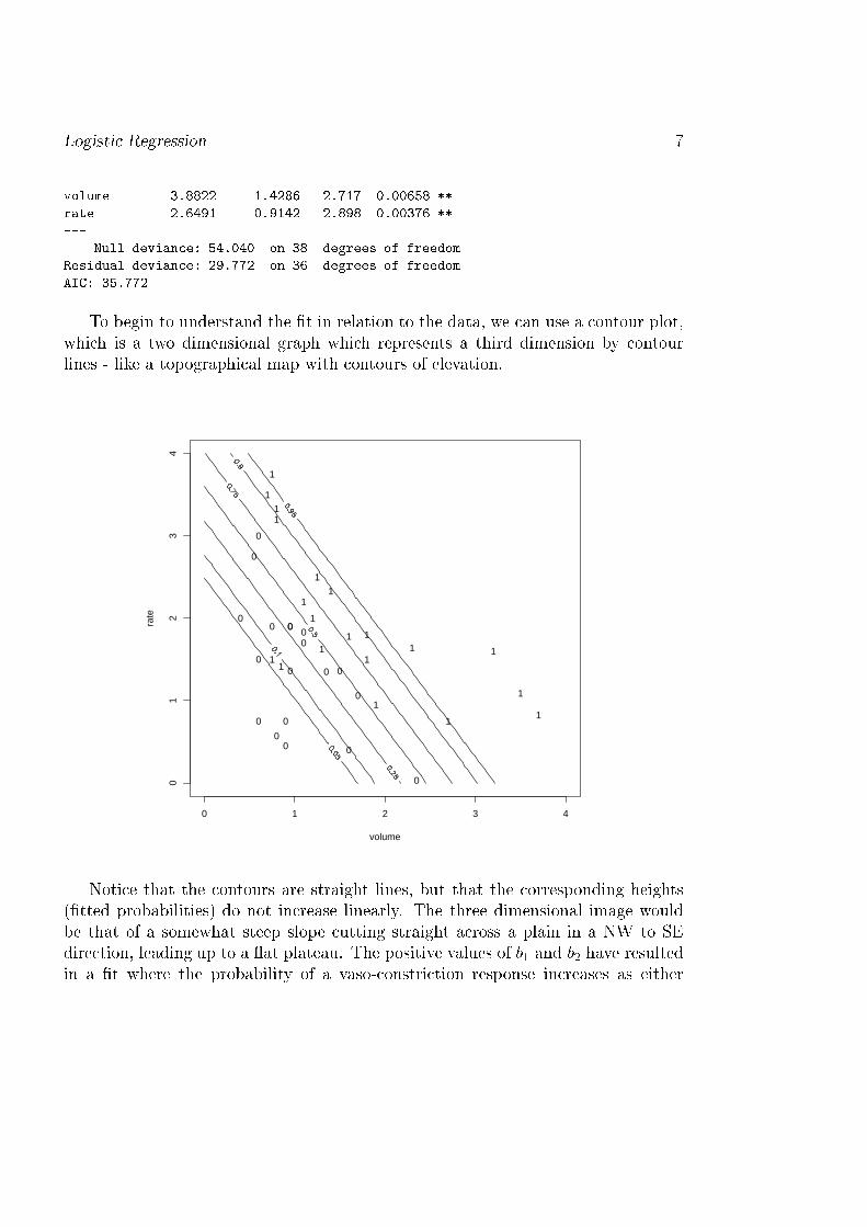
Logisti Regression 7volume 3.8822 1.4286 2.717 0.00658 **rate 2.6491 0.9142 2.898 0.00376 **--- Null devian e: 54.040 on 38 degrees of freedomResidual devian e: 29.772 on 36 degrees of freedomAIC: 35.772To begin to understand the �t in relation to the data, we an use a ontour plot,whi h is a two dimensional graph whi h represents a third dimension by ontourlines - like a topographi al map with ontours of elevation.

volume

rate

0 1 2 3 4

01

23

4

1

1

1

1

1

1

0

0

0

00

0

0

1

1

1 1

1

0

1

0

0 0 0

1

0 1

0

1

0

1

0

0

1

1

1

00

1

Noti e that the ontours are straight lines, but that the orresponding heights(�tted probabilities) do not in rease linearly. The three dimensional image wouldbe that of a somewhat steep slope utting straight a ross a plain in a NW to SEdire tion, leading up to a at plateau. The positive values of b1 and b2 have resultedin a �t where the probability of a vaso- onstri tion response in reases as either

Logisti Regression 8inspiration ow or volume in rease, with the most rapid hange o uring if both arein reased simultaneously.The plot also indi ates the a tual observed data. Note that the ases wherevaso- onstri tion o urred tend to fall on the plateau and non- onstri tion ases fallmainly on the plain (On the plain? Yes, the plain!). This indi ates that the �t isquite good.3.4 Mathemati al review: Odds and LogsBefore we delve further into the appli ation and interpretation of logisti regressionmethods, we need to review some basi mathemati s. We'll start by onsideringodds and odds ratios.3.4.1 Odds and Odds RatiosFor an event with a given probability value, p, the orresponding odds is a numeri alvalue given by oddsfEventg = p1� p:The on ept of odds �rst arose in gambling. If you bet on the o urren e of anevent (e.g. Horse A wins the ra e) and that event has a known probability, pA =PrfA winsg, then for a one dollar bet the fair return should equal the odds. Forexample, if horse A has a 50% han e of winning (pA = :5), the odds are oddsfAg =:51�:5 = 1, an equitable return on a one dollar bet is one dollar. If the horse has a25% han e of winning, the odds are :251�:25 = 1=3. For a one dollar bet, one shouldexpe t three dollars in return if the horse wins.Odds are a simple one-to-one onversion of probabilities. If presented with aprobability, it may be onverted to odds as above. If provided with odds, the onversion to probabilities follows the formula p = odds1+odds . Thus if one knows that theodds for an event are 1 in 10, i.e. .10, the probability of the event is :11+:1 = 111 � :091.Note in this instan e, the probability of .091 is nearly equal to the odds of .1.Whenever the odds are a small value, the odds be a reasonable approximation tothe probability, and vi e versa.The odds ratio is a omparative measure of two odds relative to di�erent events.For two probabilities, pA = Prfevent A o ursg and pB = Prfevent B o ursg the

Logisti Regression 9 orresponding odds of A o urring relative to B o urring isodds ratiofA vs: Bg = oddsfAgoddsfBg = pA=(1� pA)pB=(1� pB) :The "pra ti al" interpretation of an odds ratios is this. If onfronted with a hoi ebetween two wagers, one on the o urren e of A and the other on the o urren e ofB, with potential winnings of either X dollars for wager A or Y dollars for wagerB, the sound hoi e is to hoose A if odds ratiofA vs: Bg > YX .In statisti s, the odds ratio is also used as omparative measure of two proba-bilities pA and pB used as an alternative to the risk di�eren e and the relative risk.Re all the latter are de�ned by:Risk di�eren e = pA � pBRelative risk = pApBWhile these measures are somewhat more intuitive and dire tly interpretable,the odds ratio has some "mathemati al" advantages. Suppose one has ondu ts a omparative study to investigate the relationship of pA and pB. Then the relevantevents to onsider are event A, whi h orresponds to a deleterious out ome if treatedwith drug A and event B, orresponding to a deleterious out ome if treated withdrug B. The standard tabulation of the resulting data would be the two way tableof observed frequen ies:OUTCOME Deleterious Not Deleterious TotalDrugA a b a+bB d +dTotal a+ b+d nThe estimated odds ratio for A relative to B based on data as above is a�db� . Thisformula is simpler than that for the risk di�eren e = aa+b � +d or the risk ratio= a=(a+b) =( +d) . In a mathemati al sense, the odds ratio is the most natural omparativemeasure, i.e. leads to the simplest (and aestheti ally pleasing) algebra. In addi-tion, when both probabilities being ompared are small, the odds ratio will loselyapproximate the relative risk.

Logisti Regression 103.4.2 Odds and Logisti RegressionWhen a logisti relationship holds for the probability of some out ome p in relation-ship to a predi tor variable x. i.e. whenp = ea+bx1 + ea+bx ;sin e the odds relative to p equals odds1+odds , we an simply express the odds as ea+bx.Alternately we an also write that log odds = log(p=(1� p)) = a+ bx.A logisti regression relationship is thus one that is "linear in the log odds".From a mathemati al standpoint, this is the simplest hara terization of the logisti regression relationship, and is often used as the basi de�nition for su h a relation-ship. Seen from this perspe tive, the logisti regression oeÆ ients, a and b, areinterpretable as the inter ept and slope for a linear relationship between the logodds and x. From an applied perspe tive, however, log odds are not that natural to onsider.What is more natural, is to onsider the odds ratio, relative to two parti ularvalues of x, all them xA and xB. Sin e the odds are obtained by exponentiation ofthe linear formulas, the odds ratio is simplyea+bxAea+bxB :Simplifying this we have that the logarithm (natural) of the odds ratio is(a+ bxA)� (a+ bxB) = b(xA � xB) = b�x:Converting ba k from logs and using rule 3 we have that the odds ratio = (eb)�x.Thus if we exponentiate logisti regression oeÆ ients, we obtain numbers thatare interpretable in terms of odds ratios.3.4.3 An exampleIn our �rst example we revisited the ICU data and looked at the relationship betweenin-hospital mortality and initial APACHE s ore at admission to ICU. Re all thatpatients were grouped by reason for ICU admission into three groups, Monitoring,System Failure, and Emergen y admission. The table below gives the observedin-hospital mortality risk by group:

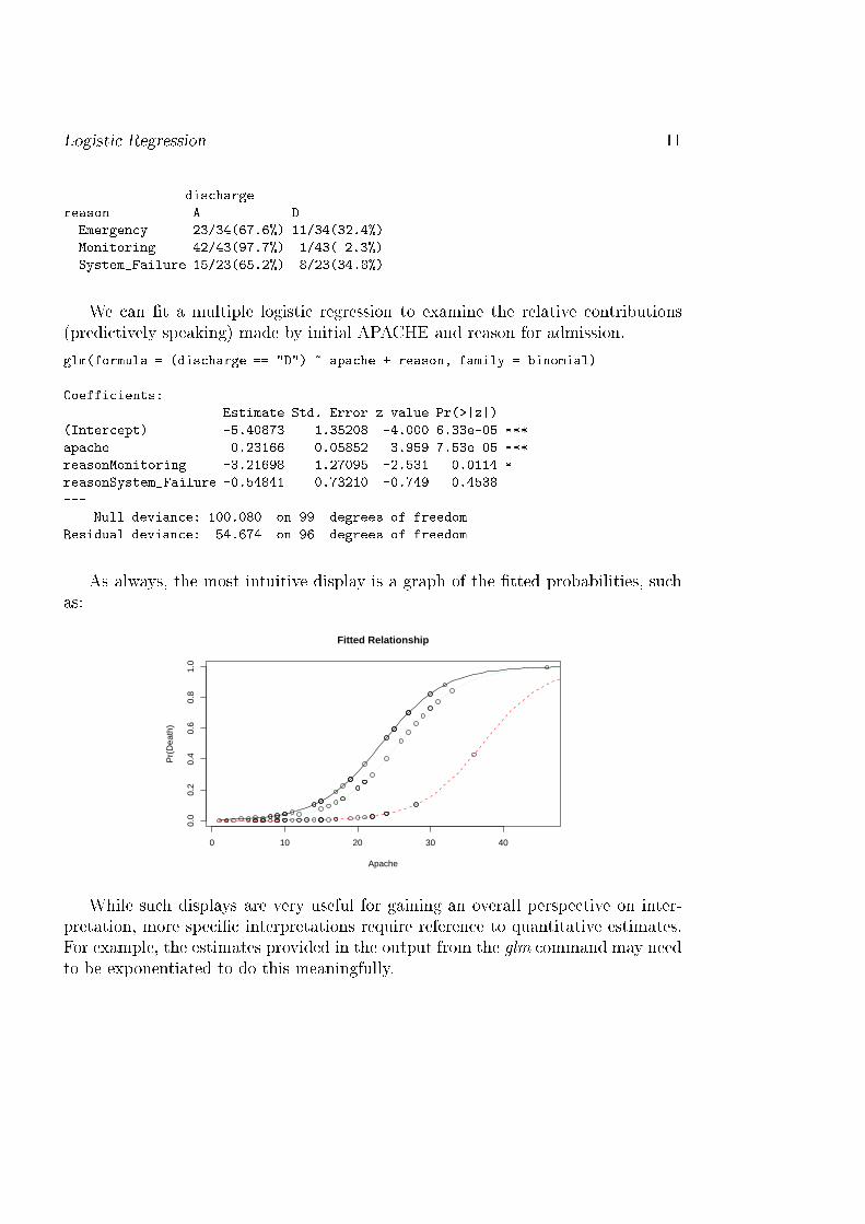
Logisti Regression 11dis hargereason A DEmergen y 23/34(67.6%) 11/34(32.4%)Monitoring 42/43(97.7%) 1/43( 2.3%)System_Failure 15/23(65.2%) 8/23(34.8%)We an �t a multiple logisti regression to examine the relative ontributions(predi tively speaking) made by initial APACHE and reason for admission.glm(formula = (dis harge == "D") ~ apa he + reason, family = binomial)Coeffi ients: Estimate Std. Error z value Pr(>|z|)(Inter ept) -5.40873 1.35208 -4.000 6.33e-05 ***apa he 0.23166 0.05852 3.959 7.53e-05 ***reasonMonitoring -3.21698 1.27095 -2.531 0.0114 *reasonSystem_Failure -0.54841 0.73210 -0.749 0.4538--- Null devian e: 100.080 on 99 degrees of freedomResidual devian e: 54.674 on 96 degrees of freedomAs always, the most intuitive display is a graph of the �tted probabilities, su has:

0 10 20 30 40

0.0

0.2

0.4

0.6

0.8

1.0

Fitted Relationship

Apache

Pr(

Dea

th)

While su h displays are very useful for gaining an overall perspe tive on inter-pretation, more spe i� interpretations require referen e to quantitative estimates.For example, the estimates provided in the output from the glm ommand may needto be exponentiated to do this meaningfully.

Logisti Regression 123.5 Logisti regression: Inferen eWe have already en ountered inferential statisti s in luding signi� an e tests and on�den e intervals in the output generated by logit and logisti . As you might sus-pe t, these quantities an be interpreted in a way analogous to orresponding valuesasso iated with linear regression output. The validity of the resulting inferen es de-pends on the underlying model assumptions, whi h for the logisti regression modelsare:Independen e: Independent observations on a binary out ome, y, are made (and oded as 0 or 1). This will o ur, for example, when we take a simple randomsample of individuals and observe a di hotomous hara teristi .Linearity of the log odds: We assume that the probability that a parti ular observa-tion, y takes on the value 1 depends on a set of explanatory variables, x1; x2; :::; xk,a ording to a linear logisti relationship, i.e.p = Probfy = 1g = e�+�1x1+�2x2+�3x3+:::+�kxk1 + e�+�1x1+�2x2+�3x3+:::+�kxkWriting this again in terms of log odds we havelog( p1� p) = �+ �1x1 + �2x2 + �3x3 + :::+ �kxkSin e log( p1�p) is also alled the logit, referen e is sometimes made to "linearity ofthe logit".Note: the �rst assumption is one whi h will depend on how the data is olle ted.Che king this assumption depends mainly on he king that a valid design was used.The se ond assumption is somewhat arti� ial, and is unlikely to be exa tly true.To he k this, we will make an empiri al examination of how well the �tted modeldes ribes the data, as we did in the linear ase.3.5.1 Sampling behaviour of the m.l.e.'sUnder the assumptions above, the maximum likelihood estimates, a; b1; b2; :::; bk areasymptoti ally optimal estimates of �; �1; �2; :::; �k (i.e. as the sample size growslarge). Thus the validity of su h likelihood-based inferen e results an only bedepended on for large sample sizes. How large is large is very diÆ ult to say. Anempiri al study 1 suggests that the observed frequen ies of y = 0 and y = 1 should1Peduzzi P. Con ato J. Kemper E. Holford TR. Feinstein AR. A simulation study of the numberof events per variable in logisti regression analysis. Journal of Clini al Epidemiology. 49(12):1373-9

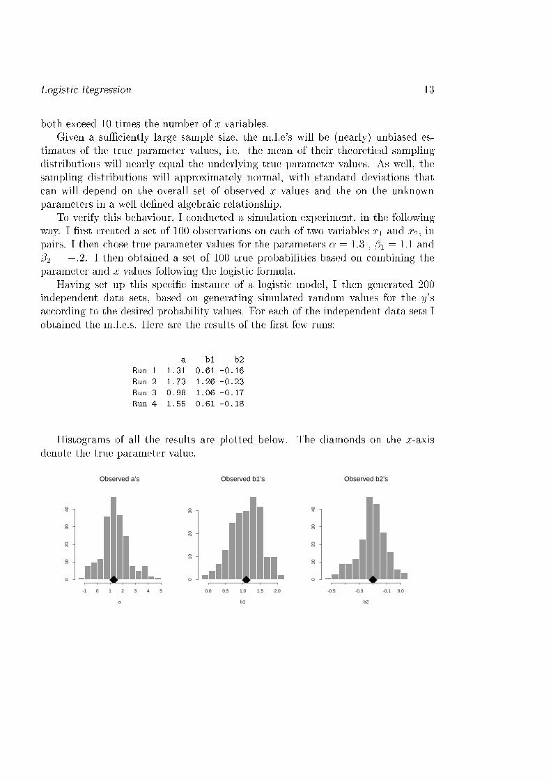
Logisti Regression 13both ex eed 10 times the number of x variables.Given a suÆ iently large sample size, the m.l.e's will be (nearly) unbiased es-timates of the true parameter values, i.e. the mean of their theoreti al samplingdistributions will nearly equal the underlying true parameter values. As well, thesampling distributions will approximately normal, with standard deviations that an will depend on the overall set of observed x values and the on the unknownparameters in a well de�ned algebrai relationship.To verify this behaviour, I ondu ted a simulation experiment, in the followingway. I �rst reated a set of 100 observations on ea h of two variables x1 and x2, inpairs. I then hose true parameter values for the parameters � = 1:3 , �1 = 1:1 and�2 = �:2. I then obtained a set of 100 true probabilities based on ombining theparameter and x values following the logisti formula.Having set up this spe i� instan e of a logisti model, I then generated 200independent data sets, based on generating simulated random values for the y'sa ording to the desired probability values. For ea h of the independent data sets Iobtained the m.l.e.s. Here are the results of the �rst few runs:a b1 b2Run 1 1.31 0.61 -0.16Run 2 1.73 1.26 -0.23Run 3 0.98 1.06 -0.17Run 4 1.55 0.61 -0.18Histograms of all the results are plotted below. The diamonds on the x-axisdenote the true parameter value.-1 0 1 2 3 4 5

010

2030

40

Observed a’s

a

0.0 0.5 1.0 1.5 2.0

010

2030

Observed b1’s

b1

-0.5 -0.3 -0.1 0.0

010

2030

40

Observed b2’s

b2

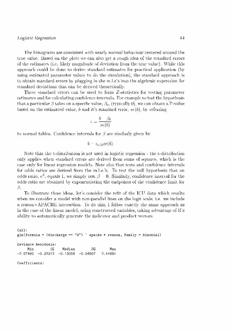
Logisti Regression 14The histograms are onsistent with nearly normal behaviour entered around thetrue value. Based on the plots we an also get a rough idea of the standard errorsof the estimates (i.e. likely magnitude of deviation from the true value). While thisapproa h ould be done to derive standard estimates for pra ti al appli ation (byusing estimated parameter values to do the simulation), the standard approa h isto obtain standard errors by plugging in the m.l.e's into the algebrai expression forstandard deviations that an be derived theoreti ally.These standard errors an be used to form Z-statisti s for testing parameterestimates and for al ulating on�den e intervals. For example to test the hypothesisthat a parti ular � takes on a spe i� value, �0, (typi ally 0), we an obtain a P-valuebased on the estimated value, b and it's standard error, se(b), by referringz = b� �0se(b)to normal tables. Con�den e intervals for � are similarly given byb� z�=2se(b):Note that the t-distribution is not used in logisti regression - the t-distributiononly applies when standard errors are derived from sums of squares, whi h is the ase only for linear regression models. Note also that tests and on�den e intervalsfor odds ratios are derived from the m.l.e.'s. To test the null hypothesis that anodds ratio, e�, equals 1, we simply test � = 0. Similarly, on�den e interval for theodds ratio are obtained by exponentiating the endpoints of the on�den e limit for�. To illustrate these ideas, let's onsider the re�t of the ICU data whi h resultswhen we onsider a model with non-parallel lines on the logit s ale, i.e. we in ludea reason�APACHE intera tion. To do this, I follow exa tly the same approa h asin the ase of the linear model, using onstru ted variables, taking advantage of R'sability to automati ally generate the indi ator and produ t ve tors.Call:glm(formula = (dis harge == "D") ~ apa he * reason, family = binomial)Devian e Residuals:Min 1Q Median 3Q Max-2.07480 -0.32312 -0.13058 -0.04507 2.44884Coeffi ients:

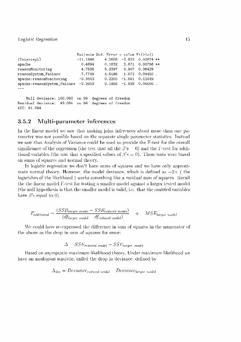
Logisti Regression 15Estimate Std. Error z value Pr(>|z|)(Inter ept) -11.1846 4.2658 -2.622 0.00874 **apa he 0.4894 0.1832 2.671 0.00756 **reasonMonitoring 4.7535 5.2397 0.907 0.36429reasonSystem_Failure 7.7749 4.6496 1.672 0.09450 .apa he:reasonMonitoring -0.3442 0.2205 -1.561 0.11849apa he:reasonSystem_Failure -0.3653 0.1988 -1.838 0.06606 .--- Null devian e: 100.080 on 99 degrees of freedomResidual devian e: 49.084 on 94 degrees of freedomAIC: 61.0843.5.2 Multi-parameter inferen esIn the linear model we saw that making joint inferen es about more than one pa-rameter was not possible based on the separate single parameter statisti s. Insteadwe saw that Analysis of Varian e ould be used to provide the F-test for the overallsigni� an e of the regression (the test that all the �'s = 0) and the F-test for addi-tional variables (the test that a spe i�ed subset of �'s = 0). These tests were basedon sums of squares and normal theory.In logisti regression we don't have sums of squares and we have only approxi-mate normal theory. However, the model devian e, whi h is de�ned as �2� ( thelogarithm of the likelihood ) works something like a residual sum of squares. Re allthe the linear model F-test for testing a smaller model against a larger tested model(the null hypothesis is that the smaller model is valid, i.e. that the omitted variableshave �'s equal to 0).Fadditional = (SSRlarger model � SSRredu ed model)(dflarger model � dfredu ed model) � MSElarger modelWe ould have re-expressed the di�eren e in sum of squares in the numerator ofthe above as the drop in sum of squares for error:� = SSEredu ed model � SSElarger modelBased on asymptoti maximum likelihood theory, Under maximum likelihood wehave an analogous statisti , alled the drop in devian e, de�ned by�dev = Devian eredu ed model �Devian elarger model

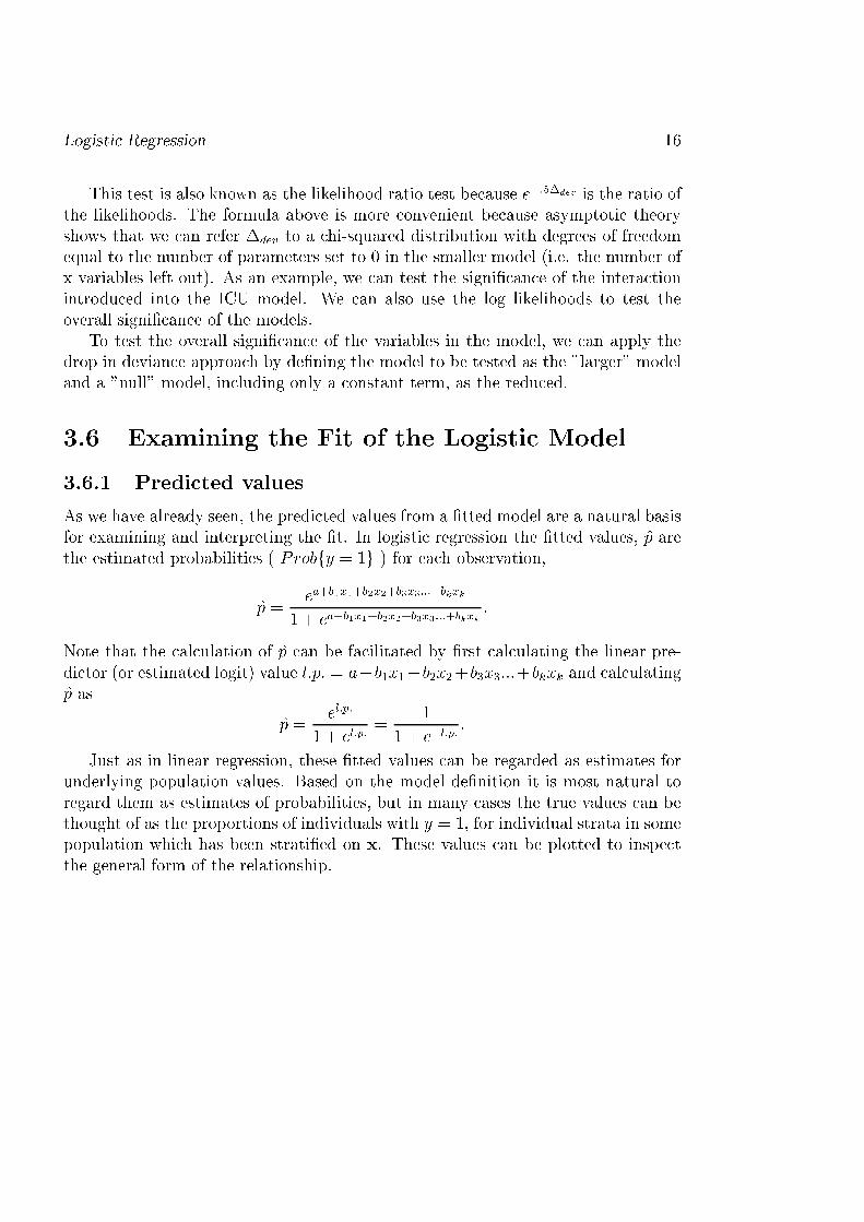
Logisti Regression 16This test is also known as the likelihood ratio test be ause e�:5�dev is the ratio ofthe likelihoods. The formula above is more onvenient be ause asymptoti theoryshows that we an refer �dev to a hi-squared distribution with degrees of freedomequal to the number of parameters set to 0 in the smaller model (i.e. the number ofx variables left out). As an example, we an test the signi� an e of the intera tionintrodu ed into the ICU model. We an also use the log likelihoods to test theoverall signi� an e of the models.To test the overall signi� an e of the variables in the model, we an apply thedrop in devian e approa h by de�ning the model to be tested as the "larger" modeland a "null" model, in luding only a onstant term, as the redu ed.3.6 Examining the Fit of the Logisti Model3.6.1 Predi ted valuesAs we have already seen, the predi ted values from a �tted model are a natural basisfor examining and interpreting the �t. In logisti regression the �tted values, p arethe estimated probabilities ( Probfy = 1g ) for ea h observation,p = ea+b1x1+b2x2+b3x3:::+bkxk1 + ea+b1x1+b2x2+b3x3:::+bkxk :Note that the al ulation of p an be fa ilitated by �rst al ulating the linear pre-di tor (or estimated logit) value l:p: = a+b1x1+b2x2+b3x3:::+bkxk and al ulatingp as p = el:p:1 + el:p: = 11 + e�l:p: :Just as in linear regression, these �tted values an be regarded as estimates forunderlying population values. Based on the model de�nition it is most natural toregard them as estimates of probabilities, but in many ases the true values an bethought of as the proportions of individuals with y = 1, for individual strata in somepopulation whi h has been strati�ed on x. These values an be plotted to inspe tthe general form of the relationship.

Logisti Regression 17F

itted

Ris

k

Fitted Risksapache

Emergency System Failure Monitoring Fitted Risk

1 46.000023

.999988

AAAAAAAAAAAAAAAAAAA

A

AAAAAAAAAAAA

D

AAAAAAAAAAAA

A

AA

A

AA

A

AAA

AA

A

A

AA

A

AADD

A

ADD

AAA

D

D

D

A

AA

DAD

AA

ADD

AA

AD

D

D

A

D

D

D

D

A

D

When regarded as estimates, it is natural to onsider the repeated samplingbehaviour of the p's. In the simulation des ribed in the previous se tion, I also kepttra k of a sele tion of p values over the two hundred repli ations. The histogramsare given below.0.2 0.3 0.4 0.5

020

4060

Observed p6’s

p6

0.2 0.3 0.4 0.5

010

2030

4050

60

Observed p8’s

p8

0.3 0.4 0.5 0.6 0.7

020

4060

Observed p61’s

p61Note the the variability of the parti ular pi is not the same for all observations- it varies with the orresponding set of x-values asso iated with the observation(whi h are onsidered to remain �xed from sample to sample - i.e. a strati�edsampling model). As in linear regression, these standard errors are smallest forobservations whose x's fall lose to the mean values for the x-variables, i.e. lose tothe "middle" of the x-data distribution. These standard errors an be used to form on�den e intervals for the true p's by using z-values, sin e the asymptoti samplingdistributions for the p's are also normal.

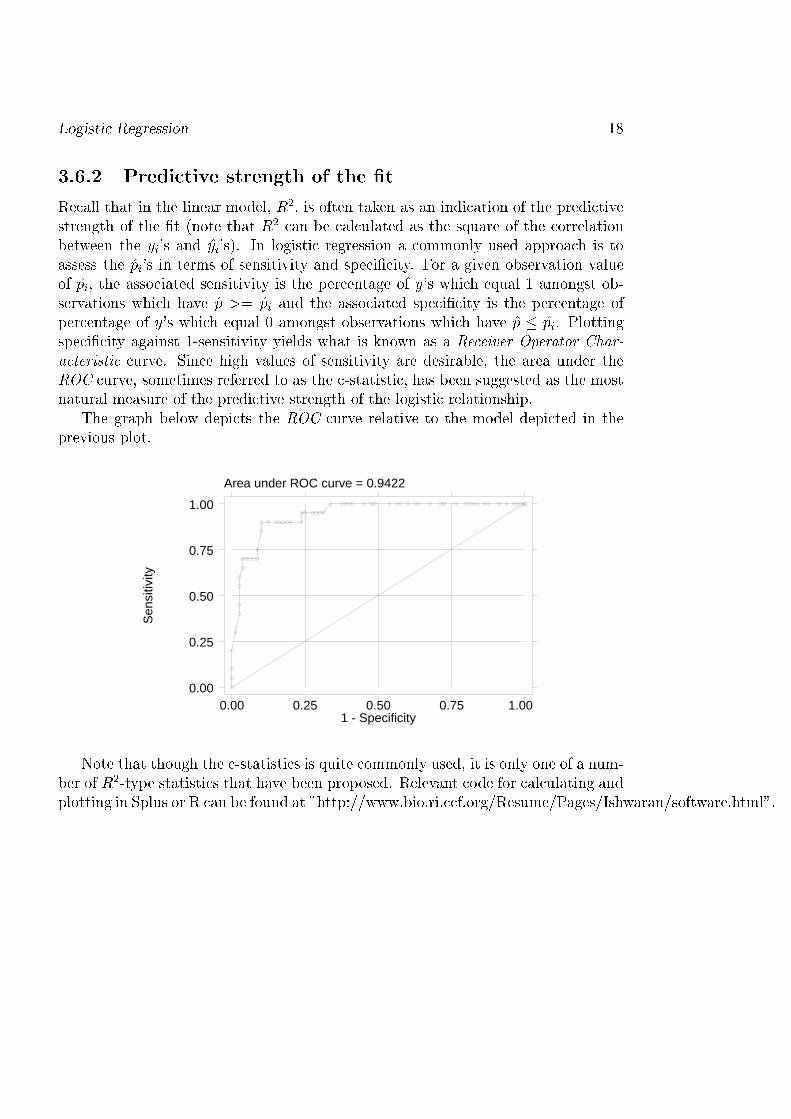
Logisti Regression 183.6.2 Predi tive strength of the �tRe all that in the linear model, R2, is often taken as an indi ation of the predi tivestrength of the �t (note that R2 an be al ulated as the square of the orrelationbetween the yi's and yi's). In logisti regression a ommonly used approa h is toassess the pi's in terms of sensitivity and spe i� ity. For a given observation valueof pi, the asso iated sensitivity is the per entage of y's whi h equal 1 amongst ob-servations whi h have p >= pi and the asso iated spe i� ity is the per entage ofper entage of y's whi h equal 0 amongst observations whi h have p � pi. Plottingspe i� ity against 1-sensitivity yields what is known as a Re eiver Operator Char-a teristi urve. Sin e high values of sensitivity are desirable, the area under theROC urve, sometimes referred to as the -statisti , has been suggested as the mostnatural measure of the predi tive strength of the logisti relationship.The graph below depi ts the ROC urve relative to the model depi ted in theprevious plot.Area under ROC curve = 0.9422

Sen

sitiv

ity

1 - Specificity0.00 0.25 0.50 0.75 1.00

0.00

0.25

0.50

0.75

1.00

Note that though the -statisti s is quite ommonly used, it is only one of a num-ber of R2-type statisti s that have been proposed. Relevant ode for al ulating andplotting in Splus or R an be found at "http://www.bio.ri. f.org/Resume/Pages/Ishwaran/software.html".

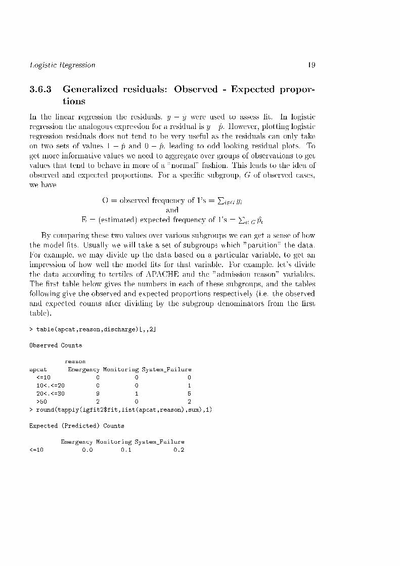
Logisti Regression 193.6.3 Generalized residuals: Observed - Expe ted propor-tionsIn the linear regression the residuals, y � y were used to assess �t. In logisti regression the analogous expression for a residual is y� p. However, plotting logisti regression residuals does not tend to be very useful as the residuals an only takeon two sets of values 1 � p and 0 � p, leading to odd looking residual plots. Toget more informative values we need to aggregate over groups of observations to getvalues that tend to behave in more of a "normal" fashion. This leads to the idea ofobserved and expe ted proportions. For a spe i� subgroup, G of observed ases,we have O = observed frequen y of 1's = Pi2G yiandE = (estimated) expe ted frequen y of 1's = Pi2G piBy omparing these two values over various subgroups we an get a sense of howthe model �ts. Usually we will take a set of subgroups whi h "partition" the data.For example, we may divide up the data based on a parti ular variable, to get animpression of how well the model �ts for that variable. For example, let's dividethe data a ording to tertiles of APACHE and the "admission reason" variables.The �rst table below gives the numbers in ea h of these subgroups, and the tablesfollowing give the observed and expe ted proportions respe tively (i.e. the observedand expe ted ounts after dividing by the subgroup denominators from the �rsttable).> table(ap at,reason,dis harge)[,,2℄Observed Countsreasonap at Emergen y Monitoring System_Failure<=10 0 0 010<.<=20 0 0 120<.<=30 9 1 5>50 2 0 2> round(tapply(lgfit2$fit,list(ap at,reason),sum),1)Expe ted (Predi ted) CountsEmergen y Monitoring System_Failure<=10 0.0 0.1 0.2

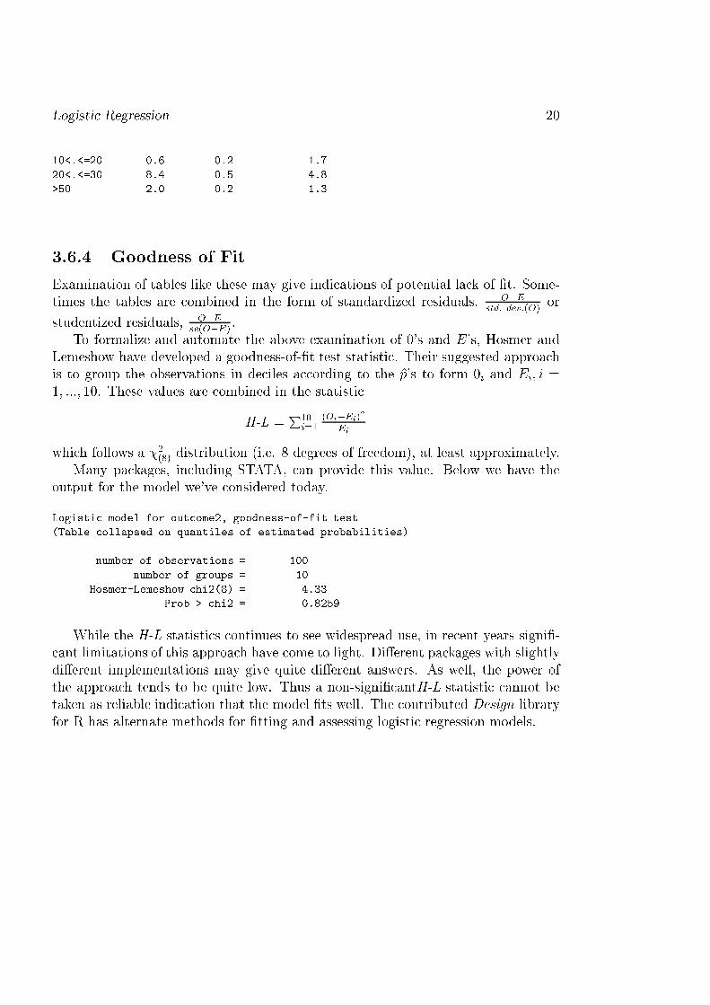
Logisti Regression 2010<.<=20 0.6 0.2 1.720<.<=30 8.4 0.5 4.8>50 2.0 0.2 1.33.6.4 Goodness of FitExamination of tables like these may give indi ations of potential la k of �t. Some-times the tables are ombined in the form of standardized residuals, O�Estd: dev:(O) orstudentized residuals, O�Ese(O�E) .To formalize and automate the above examination of 0's and E's, Hosmer andLemeshow have developed a goodness-of-�t test statisti . Their suggested approa his to group the observations in de iles a ording to the p's to form 0i and Ei; i =1; :::; 10. These values are ombined in the statisti H-L = P10i=1 (Oi�Ei)2Eiwhi h follows a �2(8) distribution (i.e. 8 degrees of freedom), at least approximately.Many pa kages, in luding STATA, an provide this value. Below we have theoutput for the model we've onsidered today.Logisti model for out ome2, goodness-of-fit test(Table ollapsed on quantiles of estimated probabilities)number of observations = 100number of groups = 10Hosmer-Lemeshow hi2(8) = 4.33Prob > hi2 = 0.8259While the H-L statisti s ontinues to see widespread use, in re ent years signi�- ant limitations of this approa h have ome to light. Di�erent pa kages with slightlydi�erent implementations may give quite di�erent answers. As well, the power ofthe approa h tends to be quite low. Thus a non-signi� antH-L statisti annot betaken as reliable indi ation that the model �ts well. The ontributed Design libraryfor R has alternate methods for �tting and assessing logisti regression models.

Logisti Regression 213.7 Sampling Design and the Logisti RegressionModelThe de�nition of the Logisti Regression model presented so far orresponds mostnaturally to data arising from either a ross-se tional or prospe tive study. Ideally inthe ross-se tional framework we take a random sample from a population, possiblystratifying on some of the explanatory (x) variables (but not on the response, y).The �tted probabilities from a logisti regression model are then best viewed asestimates of proportions in the underlying population, after strati� ation on all thex-variables.In the prospe tive ase, we begin by sele ting a set of subje ts and observingthe explanatory variables. Subje ts are then followed over some standard period,de�ned as a standard interval (e.g. 30 days) or episode (ICU stay) to determinethe response. In this ase, the �tted probabilities are estimates of the probabilityof the response o urring. (Note that if follow-up varies in an important way oversubje ts, survival methods or poisson regression should then be applied).Logisti regression is also useful in retrospe tive ase- ontrol studies, i.e. studiesin whi h out ome is �rst as ertained, separate samples of y = 0 subje ts ( ontrols)and y = 1 subje ts ( ases) are assembled, following whi h explanatory or exposuredata is olle ted. In this ase the �tted probabilities do not have a dire t interpre-tation (sin e they are largely determined by the relative sample sizes for ases and ontrols). However, odds ratios an be estimated in a valid way based on logisti re-gression. An important ex eption to this is when ases and ontrols are mat hed insets (e.g. paired design). In su h ases, a variant method alled onditional logisti regression must be applied to obtain valid estimates.3.8 Ordinal Logisti RegressionThe binary logisti regression methods we have overed in this hapter apply whenwe have a ategori al response of the simplest possible form - di hotomous. It isnatural to onsider methods for more ategori al responses having more than twopossible values. A variety of methods have been developed for overing the variouspossibilities. The best known and most highly developed are methods for ordinalresponse variables.Re all that a ategori al variable is onsidered ordinal if there is a natural or-dering of the possible values, for example Low, Medium, and High. A number ofproposed models for this type of data are extensions of the logisti regression model.

Logisti Regression 22The most well known of these ordinal logisti regression methods methods is alledthe proportional odds model.The basi idea underlying the proportional odds model is re-expressing the ate-gori al variable in terms of a number of binary variables based on internal ut-pointsin the ordinal s ale. For example, if y is a variable on a 4-point s ale, we an de�nethe orresponding binary variables, y� ; = 1; :::; 3 by y� = 1 if y > and y� if y � .If one has a set of explanatory variables, xj; j = 1; :::; k , then we an onsiderthe 3 binary logisti models orresponding to regressing ea h of the y� 's separatelyagainst the x's. The proportional odds model assumes that the true �-values arethe same in all three models, so that the only di�eren e in models is the inter eptterms, � ; = 1; 2; 3. This means that the estimates from the three binary models an be pooled to provide just one set of � estimates. By exponentiating the pooledestimate relative to a given predi tor, i.e. taking e�j , we obtain an estimate of the ommon odds ratio that des ribes the relative odds for y > for values of xj di�eringby 1 unit.Thus interpreting the proportional odds model is not mu h more diÆ ult than abinary logisti regression. However, valid intrepretations will depend on the assump-tion that proportional odds assumption, whi h must be he ked. Ordinal regressionand diagnosti methods are implemented in the ontributed Design library of R.